Adaptive conformal classification with noisy labels

Abstract

This paper develops novel conformal prediction methods for classification tasks that can automatically adapt to random label contamination in the calibration sample, enabling more informative prediction sets with stronger coverage guarantees compared to state-of-the-art approaches. This is made possible by a precise theoretical characterization of the effective coverage inflation (or deflation) suffered by standard conformal inferences in the presence of label contamination, which is then made actionable through new calibration algorithms. Our solution is flexible and can leverage different modeling assumptions about the label contamination process, while requiring no knowledge about the data distribution or the inner workings of the machine-learning classifier. The advantages of the proposed methods are demonstrated through extensive simulations and an application to object classification with the CIFAR-10H image data set.

1 Introduction

1.1 Background and motivation

Conformal inference [1] is a versatile and increasingly popular framework for estimating the uncertainty of predictions output by any supervised learning model, including for example modern deep neural networks for multi-class classification. Its two key strengths are that: (1) it requires no parametric assumptions about the data distribution, making it relevant to a variety of real-world applications; and (2) it can accommodate arbitrarily complex black-box predictive models, mitigating the risk of early obsolescence in the rapidly evolving field of machine learning. In a nutshell, conformal inference is able to transform the output of any model into a relatively informative and well-calibrated prediction set for the unknown label of a future test point, while providing precise coverage guarantees in finite samples. Intuitively, this is achieved by carefully leveraging the empirical distribution of suitable residuals (or conformity scores) evaluated on held-out data that were not utilized for training. Notably, these guarantees can be established assuming only that the calibration data are exchangeable (or, for simplicity, independent and identically distributed) random samples from the population of interest. While this framework can thus provide useful uncertainty estimates while relying on weaker assumptions compared to classical parametric modeling approaches, existing conformal prediction methods are not yet fully satisfactory for all applications. One limitation that we aim to address in this paper is the reliance on the assumption that the calibration data are labeled correctly, which is often unrealistic.

In fact, it can often be expensive to acquire accurately labeled (or clean) data, even if there is an abundance of lower-quality observations with imperfect labels [2, 3, 4, 5, 6, 7, 8, 9], which we also call noisy or contaminated. For example, the Amazon Mechanical Turk is a crowdsourcing platform that allows researchers and organizations to assign labels to large-scale unsupervised data by leveraging a global workforce of remote human annotators [10, 11]. This platform is routinely utilized across diverse fields, including for example image recognition and natural language processing. Crowdsourcing generally tends to be faster and more cost-effective compared to hiring experts, but its use has raised concerns about poor annotation quality and its impacts on the reliability of downstream analyses [12, 13, 14, 15]. While significant efforts have already been dedicated to the problem of training relatively accurate predictive models using data with low-quality labels [2, 3, 4, 5, 6, 7, 8, 9], the challenge of calibrating those models using conformal inference is largely undeveloped and has only recently begun to receive some attention [16, 17]. This paper aims to help fill such a gap.

1.2 Preview of our contributions and paper outline

This paper provides some answers to the questions of whether and how conformal inference should account for the possible presence of incorrectly labeled calibration samples, focusing on the task of constructing prediction sets for multi-class classification. After recalling the relevant technical background, we begin in Section 2 by carefully studying the impact of random label contamination on the effective coverage achieved by standard conformal prediction sets. Our analysis shows and quantifies precisely how label contamination may lead to prediction sets that are either too liberal or too conservative. The practical significance of these theoretical results becomes clear in Section 3, where we proceed to develop and study a novel calibration method that can automatically adapt to label contamination, without assuming any knowledge of the data distribution or of the classifier. As we shall see, our method can produce more informative prediction sets with more robust label-conditional coverage guarantees [18] compared to standard approaches. Initially, we assume the label contamination process is known and belongs to a broad family encompassing most of the typical models from the related literature on learning from noisy labels [2, 19, 20]. Then, we extend our solution to accommodate models that may depend on an unknown parameter, and we explain how to estimate that parameter empirically.

Section 4 extends our methods to enable the construction of adaptive prediction sets satisfying other types of theoretical guarantees, such as marginal coverage [1] and calibration-conditional coverage [21]. Further extensions encompassing even stronger guarantees, such as equalized coverage over protected categories [22], would also be possible but are omitted for length-related reasons. In Section 5, we demonstrate the practical performance of our methods through extensive numerical experiments and an analysis of the CIFAR-10H image classification data set [23]. A preview of some results is given here by Figure 1, which demonstrates that our methods are practical and produce smaller (more informative) prediction sets compared to standard conformal inference techniques, while maintaining valid coverage. Finally, Section 6 concludes with a discussion and some ideas for future work.

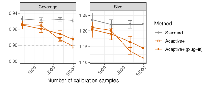
Figure 1: Performance of the proposed adaptive conformal calibration methods on CIFAR-10H image classification data with noisy human-assigned labels. The results are shown as a function of the calibration sample size and compared to the performance of standard conformal inferences, which are overly conservative due to the presence of noisy labels in the calibration data. The dashed line indicates the nominal 90% marginal coverage level.

Some content is deferred to the appendices for lack of space. Appendix A1 reviews in more detail the standard conformal prediction approach. Appendix A2 provides additional details about the proposed methods. Appendix A3 contains all mathematical proofs. Appendix A4 describes additional results from our empirical demonstrations, and Appendix A5 provides some further technical details on the setup of our numerical experiments.

1.3 Related work

Conformal inference was pioneered by Vovk and collaborators [1] in the late 1990’s and has since become a very active area of research in the statistics literature [24, 25, 26], with applications including but not limited to outlier detection [27, 28, 29, 30, 29, 31], regression [32, 33, 34], and classification [35, 36, 37, 38, 39]. Several works have studied the robustness of conformal inferences to failures of the data exchangeability assumptions [40], which may be due for example to distribution shifts [41, 42] or time-series dependencies [43, 44]. However, most prior research in conformal inference did not consider the problem of label contamination.

This paper is more closely related to [16, 17], which also considered conformal prediction sets calibrated using imperfectly labeled data in a classification setting. However, our research is distinct and involves many novelties. In fact, the problem studied by [16] is very different from ours because they allow the calibration data to contain imperfect labels but seek to predict analogous imperfect labels for the test data. By contrast, we aim to predict the true (clean) labels at test time. Our perspective is more similar to that of [17], but their efforts are focused on establishing the conservativeness of standard conformal inferences to certain forms of random label contamination, and they do not attempt to mitigate that (often excessive) conservativeness or to protect their inferences against other forms of label contamination. Our theoretical analyses take a different approach, leading to more general and quantitative results that hold for a broader class of contamination models. Then, our main contribution is to develop novel methods that can automatically adapt to label contamination. To the best of our knowledge, this is the first work to propose conformal prediction methods that are adaptive to label contamination.

2 Preliminaries

2.1 Problem statement

Consider $n+1$ data points $(X_{i},Y_{i},\tilde{Y}_{i})$, for $i\in[n+1]=\{1,\ldots,n+1\}$, where $X_{i}\in\mathbb{R}^{d}$ is a feature vector, $Y_{i}\in[K]$ is a latent categorical label, and $\tilde{Y}_{i}\in[K]$ is an observable label that we interpret as a contaminated version of $Y_{i}$. Assume the data are i.i.d. random samples from some unknown distribution. A weaker exchangeability assumption often turns out to be sufficient in the related literature, but we focus on i.i.d. data in this paper. The problem we consider is that of constructing informative conformal prediction sets for the true label $Y_{n+1}$ of a test point with features $X_{n+1}$, leveraging the available observations $(X_{i},\tilde{Y}_{i})$ indexed by $[n]$, to which we collectively refer as $\mathcal{D}$. Of course, in order to establish precise coverage guarantees, it will be necessary to introduce some assumptions about the relation between the true and contaminated labels, as we shall see. Our setup thus extends the standard conformal prediction framework for uncontaminated data, which corresponds to the special case in which $\tilde{Y}=Y$ almost surely.

2.2 Relevant technical background

This section recalls some relevant background on standard conformal classification methods, which ignore the possibility of label contamination. Our notation is inspired by that of [38], although it also involves some changes that will be helpful to present our novel methods. Note that we will refer to standard conformal prediction approaches as working with observations $(X,\tilde{Y})$ in order to keep our notation consistent, but it should be kept in mind that the prior literature typically did not distinguish between $Y$ and $\tilde{Y}$.

Let $\mathcal{A}$ denote any machine learning algorithm for classification; e.g., a logistic regression model or a neural network. This may be a complex algorithm and it is treated as a black-box throughout the paper. The role of $\mathcal{A}$ is to train a model $\hat{\pi}$ that estimates the unknown distribution of $\tilde{Y}\mid X$ using the observations $(X_{i},\tilde{Y}_{i})$ in $\mathcal{D}$. For any $k\in[K]$ and $x\in\mathbb{R}^{d}$, define $\hat{\pi}(x,k)\in[0,1]$ as the estimated probability that a sample with features $X=x$ has an observable label $\tilde{Y}=k$. In the following, it will sometimes be convenient to assume that the distribution of $\hat{\pi}(X,k)$ is continuous, so that there are almost surely no ties. This condition could be relaxed at the cost of a more involved notation, but it can be made realistic by simply adding a small amount of independent noise to the output of the model. Further, we assume that $\hat{\pi}$ is normalized, in the sense that $\sum_{k=1}^{K}\hat{\pi}(x,k)=1$. Aside from these requirements, we allow $\hat{\pi}$ to be anything and do not necessarily expect it to model the true distribution of $\tilde{Y}\mid X$ accurately. Thus, typical off-the-shelf classifiers can provide suitable statistics $\hat{\pi}$ by default. For example, one may choose $\hat{\pi}$ to be the output of the final soft-max layer of a deep neural network trained to minimize the cross-entropy loss.

This paper will study how to translate the aforementioned black-box model into a reliable prediction set for the label $Y_{n+1}$ of a test point with features $X_{n+1}$. But first we need to review the standard conformal inference approach to the simpler special case where $Y=\tilde{Y}$. The first key notion that we need to recall is that of a prediction function.

Definition 1 (Prediction function).

Let $\mathcal{C}$ be a set-valued function, whose form may depend on the model $\hat{\pi}$, that takes as input $x\in\mathbb{R}^{d}$ and $\tau=(\tau_{1},\ldots,\tau_{K})\in[0,1]^{K}$, and returns as output a subset of $[K]$. We say that $\mathcal{C}$ is a prediction function if it is monotone increasing with respect to each element of $\tau$ and satisfies $k\in\mathcal{C}(X,\tau)$ whenever $\tau_{k}=1$, for any $k\in[K]$.

Note that the dependence of a prediction function $\mathcal{C}$ on $\hat{\pi}$ will typically be kept implicit unless otherwise necessary to avoid ambiguity; i.e., $\mathcal{C}(x,\tau)=\mathcal{C}(x,\tau;\hat{\pi})\subseteq[K]$.

For any prediction function $\mathcal{C}$, we define the associated conformity score function $\hat{s}:\mathbb{R}^{d}\times[K]\mapsto[0,1]$, also implicitly depending on $\hat{\pi}$, as that function which outputs the smallest value of $\tau_{k}$ allowing the label $k$ to be contained in the set $\mathcal{C}(x,\tau_{k})$. That is,

$$\hat{s}(x,k)=\inf\left\{\tau_{k}\in[0,1]:k\in\mathcal{C}(x,\tau_{k})\right\}.$$ (1)

Note that the short-hand $\mathcal{C}(X,\tau_{k})$ above is a slight abuse of notation, since $\mathcal{C}$ was defined for a vector-valued input $\tau$, but it does not introduce any ambiguity because the event $k\in\mathcal{C}(x,\tau)$ only depends on the value of the $k$-th component of $\tau$.

A classical example of $\mathcal{C}$ is the function that outputs the set of all labels $k\in[K]$ for which the estimated conditional probability of $\tilde{Y}=k\mid X=x$ is sufficiently large; i.e.,

$$\mathcal{C}(x,\tau;\hat{\pi}) :=\{k\in[K]:\hat{\pi}_{k}(x)\geq 1-\tau_{k}\}.$$ (2)

The associated scores are given by $\hat{s}(x,k)=1-\hat{\pi}_{k}(x)$. These are sometimes called homogeneous conformity scores because the prediction function in (2) is not designed to account for heteroscedasticity in the distribution of $Y\mid X$ [37, 38]. While this choice of $\mathcal{C}$ can be convenient to keep the notation as simple as possible, it is important to emphasize that all of our results also extend to other prediction functions, including those associated with the generalized inverse quantile conformity scores of [38], which we review in Appendix A1.

A standard implementation of conformal inference begins by randomly splitting the labeled data into two disjoint subsets, $\mathcal{D}^{\text{train}}$ and $\mathcal{D}^{\mathrm{cal}}$, such that $\mathcal{D}=\mathcal{D}^{\text{train}}\cup\mathcal{D}^{\mathrm{cal}}$. The model $\hat{\pi}$ is trained using the data in $\mathcal{D}^{\text{train}}$. The hold-out observations in $\mathcal{D}^{\mathrm{cal}}$ are utilized to compute conformity scores $\hat{s}(X_{i},k)$ via (1), for all $k\in[K]$ and $i\in\mathcal{D}^{\mathrm{cal}}$, according to the desired prediction function $\mathcal{C}$. These scores are then utilized to calibrate a prediction set for a new test point with features $X_{n+1}$ as follows. For each $k\in[K]$, define $\mathcal{D}_{k}^{\mathrm{cal}}=\{i\in\mathcal{D}^{\mathrm{cal}}:\tilde{Y}_{i}=k\}$, $n_{k}=|\mathcal{D}_{k}^{\mathrm{cal}}|$, and $\hat{\tau}=(\hat{\tau}_{1},\ldots,\hat{\tau}_{K})$, where

$$\hat{\tau}_{k}=\lceil(1+n_{k})\cdot(1-\alpha)\rceil\text{-th smallest value in }\{\hat{s}(X_{i},k)\}_{i\in\mathcal{D}_{k}^{\mathrm{cal}}},$$ (3)

and $\alpha\in(0,1)$ is the desired significance level. Finally, the calibrated prediction set for the unknown test label $Y_{n+1}$ is given by $\hat{C}(X_{n+1})=\mathcal{C}(X_{n+1},\hat{\tau};\hat{\pi})$. See Algorithm 4 in Appendix A1.2 for a summary of this method. This procedure makes it possible to prove that $\hat{C}(X_{n+1})$ has label-conditional coverage [18] at level $1-\alpha$ in finite samples,

$$\mathbb{P}\left[Y_{n+1}\in\hat{C}(X_{n+1})\mid Y_{n+1}=k\right]\geq 1-\alpha,\qquad\text{ for all }k\in[K],$$ (4)

as long as $Y=\tilde{Y}$ almost surely. See Proposition A1 for a formal statement of this result, which also provides an almost-matching coverage upper bound. Note that the probability in (4) is taken with respect to the features $X_{n+1}$ of the test point as well as the labeled data in $\mathcal{D}$, both of which are treated as random. In the following sections, we will study the behavior of this method in more depth while allowing $\tilde{Y}\neq Y$.

In the meantime, we recall that an alternative approach in conformal inference is to construct prediction sets $\hat{C}(X_{n+1})$ satisfying the following weaker notion of marginal coverage:

$$\mathbb{P}\left[Y_{n+1}\in\hat{C}(X_{n+1})\right]\geq 1-\alpha.$$ (5)

As long as $Y=\tilde{Y}$ almost surely, prediction sets with marginal coverage can be obtained by simply replacing the subset $\mathcal{D}_{k}^{\mathrm{cal}}$ with $\mathcal{D}^{\mathrm{cal}}$ in Algorithm 4. See Algorithm 5 and Proposition A2 in Appendix A1.3 for further details. While marginal coverage (5) is not as strong as label-conditional coverage (4), it is a useful notion because it is easier to achieve using smaller and hence more informative prediction sets. Therefore, we will study how to efficiently control both (5) and (4) using contaminated data, leaving it to practitioners to determine which coverage guarantee is most appropriate for any particular application.

2.3 General coverage bounds under label contamination

This section analyzes theoretically the behaviour of standard conformal classification approaches applied with contaminated calibration data. In particular, we demonstrate how label noise can cause the effective coverage achieved by these methods to be either inflated or deflated, as made precise by an explicit factor that depends on the distribution of the conformity scores. For simplicity, we first focus on label-conditional coverage (4), studying the behavior of Algorithm 4. Then, we extend those results to study the behavior of Algorithm 5, which targets marginal coverage (5).

It is worth emphasizing that the results presented in this section require no assumptions on the contamination process and encompass a wide range of scenarios in which label noise leads to over-coverage or under-coverage; thus, our analysis is much more general than that of [17], which focused on establishing conservativeness under a narrower random corruption model. That being said, it will become clear in the next section that some assumptions about the contamination model are useful to achieve the more ambitious goal of developing practical conformal prediction methods that can automatically adapt to label noise.

The following notation will be helpful. For any $k,l\in[K]$ and $t\in\mathbb{R}$, define

$$\begin{split}F_{l}^{k}(t)&:=\mathbb{P}\left[\hat{s}(X,k)\leq t\mid Y=l,\mathcal{D}^{\text{train}}\right],\\ \tilde{F}_{l}^{k}(t)&:=\mathbb{P}\left[\hat{s}(X,k)\leq t\mid\tilde{Y}=l,\mathcal{D}^{\text{train}}\right].\end{split}$$ (6)

In words, $F_{l}^{k}$ is the cumulative distribution function of $\hat{s}(X,k)$, based on a fixed function $\hat{s}$ and a random sample $X$ from the distribution of $X\mid Y=l$, namely $P_{l}$. Analogously, $\tilde{F}_{l}^{k}$ is the cumulative distribution function corresponding to a random sample $X$ from the distribution of $X\mid\tilde{Y}=l$, namely $\tilde{P}_{l}$. For any $k\in[K]$ and $t\in\mathbb{R}$, define also $\Delta_{k}(t)$ as

$$\Delta_{k}(t) :=F_{k}^{k}(t)-\tilde{F}_{k}^{k}(t).$$ (7)

We will refer to $\Delta_{k}(t)$ as the coverage inflation factor because its expected value controls the discrepancy between the real and nominal label-conditional coverage of the prediction sets output by Algorithm 4, as established by the next result. Note that $\Delta_{k}(t)$ may be either positive or negative.

Theorem 1.

Suppose $(X_{i},Y_{i},\tilde{Y}_{i})$ are i.i.d. for all $i\in[n+1]$. Fix any prediction function $\mathcal{C}$ satisfying Definition 1, and let $\hat{C}(X_{n+1})$ indicate the prediction set output by Algorithm 4 applied using the corrupted labels $\tilde{Y}_{i}$ instead of the clean labels $Y_{i}$, for all $i\in[n]$. Then,

$$\mathbb{P}\left[Y_{n+1}\in\hat{C}(X_{n+1})\mid Y_{n+1}=k\right]\geq 1-\alpha+\mathbb{E}\left[\Delta_{k}({\widehat{\tau}}_{k})\right].$$ (8)

Further, if the conformity scores $s(X_{i},\tilde{Y}_{i})$ used by Algorithm 4 are almost-surely distinct,

$$\mathbb{P}\left[Y_{n+1}\in\hat{C}(X_{n+1})\mid Y_{n+1}=k\right]\leq 1-\alpha+\frac{1}{n_{k}+1}+\mathbb{E}\left[\Delta_{k}({\widehat{\tau}}_{k})\right].$$ (9)

Note that, above, $\mathbb{E}\left[\Delta_{k}({\widehat{\tau}}_{k})\right]$ denotes an expected value taken with respect to the randomness in the data $\mathcal{D}$ used to calculate the threshold ${\widehat{\tau}}_{k}$. This result tells us that standard conformal inferences may be either overly conservative or too liberal when dealing with contaminated data, depending on whether $\mathbb{E}\left[\Delta_{k}({\widehat{\tau}}_{k})\right]$ is positive or negative.

A similar result can also be reached about the marginal coverage of the prediction sets produced by Algorithm 5. In this case, a useful quantity to define, for any $t\in[0,1]$, is the marginal coverage inflation factor,

$$\Delta(t) :=\sum_{k=1}^{K}\left[\rho_{k}F_{k}^{k}(t)-\tilde{\rho}_{k}\tilde{F}_{k}^{k}(t)\right]=F(t)-\tilde{F}(t),$$ (10)

where $\rho_{k}:=\mathbb{P}[Y=k]$ and $\tilde{\rho}_{k}=\mathbb{P}[\tilde{Y}=k]$ indicate the expected proportions of clean and corrupted labels equal to $k$, respectively. Above, $F(t)$ and $\tilde{F}(t)$ are the marginal cumulative distribution functions of $\hat{s}(X,Y)$ and $\hat{s}(X,\tilde{Y})$, respectively, conditional on $\mathcal{D}$; i.e.,

$$F^{k}(t):=\mathbb{P}\left[\hat{s}(X,Y)\leq t\mid\mathcal{D}^{\text{train}}\right], \tilde{F}^{k}(t):=\mathbb{P}\left[\hat{s}(X,\tilde{Y})\leq t\mid\mathcal{D}^{\text{train}}\right].$$

Theorem 2.

Suppose $(X_{i},Y_{i},\tilde{Y}_{i})$ are i.i.d. for all $i\in[n+1]$. Fix any prediction function $\mathcal{C}$ satisfying Definition 1, and let $\hat{C}(X_{n+1})$ indicate the prediction set output by Algorithm 5 applied using the corrupted labels $\tilde{Y}_{i}$ instead of the clean labels $Y_{i}$, for all $i\in[n]$. Then,

$$\mathbb{P}\left[Y_{n+1}\in\hat{C}(X_{n+1})\right]\geq 1-\alpha+\mathbb{E}\left[\Delta({\widehat{\tau}})\right].$$ (11)

Further, if the conformity scores $s(X_{i},\tilde{Y}_{i})$ used by Algorithm 5 are almost-surely distinct,

$$\mathbb{P}\left[Y_{n+1}\in\hat{C}(X_{n+1})\right]\leq 1-\alpha+\frac{1}{n_{\mathrm{cal}}+1}+\mathbb{E}\left[\Delta({\widehat{\tau}})\right].$$ (12)

These results serve as the starting point of the next section, which introduces additional modeling assumptions about the label contamination process and sheds more light onto the situations in which standard conformal inferences can be guaranteed to be conservative.

2.4 Coverage lower bounds under a linear contamination model

To obtain more interpretable and actionable expressions for the coverage bounds presented in the previous section, one must introduce some assumptions about the relation between the latent labels $Y$ and the observable labels $\tilde{Y}$. Fortunately, significant progress can be made by simply assuming that $\tilde{Y}$ is conditionally independent of $X$ given $Y$. This corresponds to a widely used class of label contamination models [2, 20].

Assumption 1.

$\tilde{Y}\mathchoice{\mathrel{\hbox to0.0pt{$\displaystyle\perp$\hss}\mkern 2.0mu{\displaystyle\perp}}}{\mathrel{\hbox to0.0pt{$\textstyle\perp$\hss}\mkern 2.0mu{\textstyle\perp}}}{\mathrel{\hbox to0.0pt{$\scriptstyle\perp$\hss}\mkern 2.0mu{\scriptstyle\perp}}}{\mathrel{\hbox to0.0pt{$\scriptscriptstyle\perp$\hss}\mkern 2.0mu{\scriptscriptstyle\perp}}}X\mid Y$.

A consequence of 1 is that it gives rise to a convenient relation between the conditional distribution of $X\mid\tilde{Y}=k$, namely $\tilde{P}_{k}$, and the conditional distributions of $X\mid Y=l$, namely $P_{l}$, for all $k,l\in[K]$. In plain words, for any $k\in[K]$, the distribution $\tilde{P}_{k}$ is a linear mixture of the distributions $P_{l}$ for all $l\in[K]$.

Proposition 1.

Let $M$ be a $K\times K$ matrix such that $M_{kl}=\mathbb{P}[Y=l\mid\tilde{Y}=k]$ for any $k,l\in[K]$. Then, 1 implies that

$$\tilde{P}_{k}=\sum_{l=1}^{K}M_{kl}P_{l}.$$ (13)

This mixture model extends the classical binary class-dependent noise model in [19] to the multi-class setting. Further, following the same approach as in the proof of Proposition 1, one can verify that 1 also implies: $\mathbb{P}[\tilde{Y}=k\mid X,Y=l]=M_{kl}\tilde{\rho}_{k}/\rho_{l}$. In the special case of $M_{kl}=\eta/(K-1)$ for all $k\neq l$, where $0\leq\eta\leq 1$, and $\rho_{k}=\tilde{\rho}_{k}=1/K$ for all $k\in[K]$, this model reduces to the simple homogeneous noise setting [20].

Proposition 1 is useful to prove that, under 1, standard conformal inferences can be guaranteed to be conservative as long as an additional stochastic dominance condition about the distributions of the conformity scores holds.

Corollary 1.

Consider the same setting of Theorem 1 and assume 1 holds. Suppose also that the cumulative distribution functions of the conformity scores (6) satisfy

$$\max_{l\neq k}F_{l}^{k}(t)\leq F_{k}^{k}(t),$$ (14)

for all $t\in\mathbb{R}$ and $k\in[K]$. Then, $\Delta_{k}(\hat{\tau}_{k})\geq 0$ almost-surely for any $k\in[K]$, and hence the predictions sets $\hat{C}(X_{n+1})$ output by Algorithm 4 satisfy (4).

Intuitively, Equation (14) states that the trained model tends to assign smaller scores $\hat{s}(X,k)$ to data points with true label $Y=k$. In the special case of $\hat{s}(X,k)=1-\hat{\pi}_{k}(X)$, this becomes equivalent to $\mathbb{E}\left[\phi(\hat{\pi}_{k}(X))\mid Y=k,\mathcal{D}^{\text{train}}\right]\leq\mathbb{E}\left[\phi(\hat{\pi}_{k}(X))\mid Y=l,\mathcal{D}^{\text{train}}\right]$ for any $l,k\in[K]$ and any monotone increasing function $\phi$. In other words, Equation (14) requires the model to estimate the conditional distribution of $Y\mid X$ sufficiently accurately as to at least preserve the relative ranking of the most likely labels, on average.

The same stochastic dominance condition as in Corollary 1 also implies that the prediction sets output of Algorithm 5 are conservative in the marginal coverage sense of (5).

Corollary 2.

Consider the same setting of Theorem 2 and assume 1 holds. Suppose also that the cumulative distribution functions of the conformity scores (6) satisfy

$$\max_{l\neq k}F_{k}^{l}(t)\leq F_{k}^{k}(t),$$ (15)

for all $t\in\mathbb{R}$ and $k\in[K]$. Then, $\Delta(\hat{\tau})\geq 0$ almost-surely, and hence the predictions $\hat{C}(X_{n+1})$ of Algorithm 5 satisfy (5).

Equation (15) is similar to (14), although the two conditions are not exactly equivalent. Intuitively, (15) states that the scores $\hat{s}(X,k)$ assigned by the machine learning model tend to be smaller than any other scores $\hat{s}(X,l)$ for $l\neq k$ among data points with true label $Y=k$. In other words, this could be interpreted as saying that the correct label is the most likely point prediction of the machine learning model, for each possible class $k\in[K]$.

In summary, Corollaries 1 and 2 provide lower bounds that highlight a certain robustness of standard conformal inferences to label contamination, consistently with [17]. However, these results are not yet fully satisfactory for at least two reasons. Firstly, it is unclear how to check whether the stochastic dominance assumption (14) holds in practice. Secondly, even if (14) is satisfied, one may be concerned that standard conformal inferences can be too conservative under label contamination, leading to unnecessarily large prediction sets. This is why we develop in the next section novel conformal inference methods that can automatically adapt to label contamination, producing informative prediction sets that rigorously guarantee coverage at the desired level.

3 Methodology

3.1 Adaptive coverage under known label contamination

This section presents a novel method for constructing conformal prediction sets that can automatically adapt to label contamination. For simplicity, we begin by focusing on achieving tight label-conditional coverage under the assumption that the label contamination model is known. Subsequently, similar ideas will be extended to accommodate label contamination models with an unknown parameter, or to provide other coverage guarantees.

3.1.1 A plug-in estimate for the coverage inflation factor

The proposed method will leverage 1 through Proposition 1, which makes it possible to write the inflation factor $\Delta_{k}(t)$ in (7) in terms of quantities that are either known or estimable. In fact, as long as $M$ in (13) admits a matrix inverse $V=M^{-1}$, the factor $\Delta_{k}(t)$ can be equivalently expressed as:

$$\Delta_{k}(t) =(V_{kk}-1)\tilde{F}_{k}^{k}(t)+\sum_{l\neq k}V_{kl}\tilde{F}_{l}^{k}(t).$$

This expression only depends on the inverse matrix $V$, which is assumed to be known, and on the distribution of $\tilde{Y}$, which is observable. This intuitively suggests that it may be possible to estimate $\Delta_{k}(t)$ from the available data and then leverage Theorem 1 to obtain an adaptive conformal inference method with tighter coverage guarantees compared to the standard approach studied in Section 2. In the following, we develop such a method and establish both upper and lower bounds for its coverage under the general linear mixture contamination model defined in (13), assuming for simplicity that $M$ is known. The problem of estimating $M$ will then be addressed later.

The proposed method begins by randomly splitting the labeled data into two disjoint subsets, $\mathcal{D}^{\text{train}}$ and $\mathcal{D}^{\mathrm{cal}}$, similarly to standard conformal inference, The observations in $\mathcal{D}^{\text{train}}$ are used to train the model $\hat{\pi}$, while those in $\mathcal{D}^{\mathrm{cal}}$ are used to compute conformity scores $\hat{s}(X_{i},k)$ via (1), for all $k\in[K]$ and $i\in\mathcal{D}^{\mathrm{cal}}$, according to the desired prediction function $\mathcal{C}$. For any $k,l\in[k]$, let $\hat{F}_{l}^{k}$ denote the empirical cumulative distribution function of $\hat{s}(X_{i},k)$ for $i\in\mathcal{D}_{l}^{\mathrm{cal}}=\{i\in\mathcal{D}^{\mathrm{cal}}:\tilde{Y}_{i}=l\}$; i.e.,

$$\hat{F}_{l}^{k}(t):=\frac{1}{n_{l}}\sum_{i\in\mathcal{D}_{l}^{\mathrm{cal}}}\mathbb{I}\left[\hat{s}(X_{i},k)\leq t\right],$$ (16)

where $n_{l}=|\mathcal{D}_{l}^{\mathrm{cal}}|$. In other words, $\hat{F}_{l}^{k}(t)$ is the intuitive empirical estimate of $\tilde{F}_{l}^{k}$. If the parameter matrix $V$ of the label contamination model described in the previous section is known, one can leverage the $\hat{F}_{l}^{k}$ functions to compute a plug-in estimate $\hat{\Delta}_{k}(t)$ of the coverage inflation factor $\Delta_{k}(t)$:

$$\hat{\Delta}_{k}(t) :=(V_{kk}-1)\hat{F}_{k}^{k}(t)+\sum_{l\neq k}V_{kl}\hat{F}_{l}^{k}(t).$$ (17)

If one believed that the function $\hat{\Delta}_{k}$ can estimate $\Delta_{k}$ accurately, one would guess from Theorem 1 that Algorithm 4—the standard conformal inference method that ignores label contamination—leads to an effective coverage close to $1-\alpha+\hat{\Delta}_{k}(\hat{\tau}_{k})$, where $\hat{\tau}_{k}$ is the data-driven calibration parameter computed via (3). Informally speaking, this observation suggests adjusting the nominal significance level to something close to $\alpha-\hat{\Delta}_{k}(\hat{\tau}_{k})$ in order to achieve $1-\alpha$ coverage. We will now translate this intuition into a rigorous method.

3.1.2 The adaptive calibration algorithm

For any $k\in[K]$, define the set $\hat{\mathcal{I}}_{k}\subseteq\mathcal{D}_{k}^{\mathrm{cal}}$ as

$$\hat{\mathcal{I}}_{k}:=\left\{i\in[n_{k}]:\frac{i}{n_{k}}\geq 1-\alpha-{\widehat{\Delta}}_{k}(S^{k}_{(i)})+\delta(n_{k},n_{*})\right\},$$ (18)

where $S^{k}_{(i)}$, for $i\in[n_{k}]$, are the order statistics of $\{\hat{s}(X_{j},k)\}_{j\in\mathcal{D}_{j}^{\mathrm{cal}}}$, while $n_{*}:=\min_{k\in[K]}n_{k}$, and $\delta(n_{k},n_{*})$ is a finite-sample correction factor that will be specified later. Our threshold $\hat{\tau}_{k}$ is then given by:

$$\hat{\tau}_{k} =\begin{cases}S^{k}_{(\hat{i}_{k})}\text{ where }\hat{i}_{k}=\min\{i\in\hat{\mathcal{I}_{k}}\},&\text{if }\hat{\mathcal{I}}_{k}\neq\emptyset,\\ 1,&\text{if }\hat{\mathcal{I}}_{k}=\emptyset.\end{cases}$$ (19)

Finally, the prediction set output by our proposed method is $\hat{C}(X_{n+1})=\mathcal{C}(X,\hat{\tau})$, where $\hat{\tau}=(\hat{\tau}_{1},\ldots,\hat{\tau}_{K})$. This procedure is outlined in Algorithm 1.

1

Input: Data set $\{(X_{i},\tilde{Y}_{i})\}_{i=1}^{n}$ with corrupted labels $\tilde{Y}_{i}\in[K]$.

         The inverse $V$ of the matrix $M$ in (13).

         Unlabeled test point with features $X_{n+1}$.

         Machine learning algorithm $\mathcal{A}$ for training a $K$-class classifier.

         A valid prediction function $\mathcal{C}$ satisfying Definition 1; e.g., (2).

         Desired coverage level $1-\alpha\in(0,1)$.

2

3Randomly split $[n]$ into two disjoint subsets, $\mathcal{D}^{\text{train}}$ and $\mathcal{D}^{\mathrm{cal}}$.

4 Train the classifier $\mathcal{A}$ on the data in $\mathcal{D}^{\text{train}}$.

5 Compute conformity scores $\hat{s}(X_{i},k)$ using (1) for all $i\in\mathcal{D}^{\mathrm{cal}}$ and all $k\in[K]$.

6 Define the empirical CDF $\hat{F}_{l}^{k}$ of $\{\hat{s}(X_{i},k):i\in\mathcal{D}_{l}^{\mathrm{cal}}\}$ for all $l\in[K]$, as in (16).

7 for $k=1,\dots,K$ do

8       Define $\mathcal{D}_{k}^{\mathrm{cal}}=\{i\in\mathcal{D}^{\mathrm{cal}}:\tilde{Y}_{i}=k\}$ and $n_{k}=|\mathcal{D}_{k}^{\mathrm{cal}}|$.

9       Sort the scores $\{\hat{s}(X_{i},k):i\in\mathcal{D}_{k}^{\mathrm{cal}}\}$ into $(S^{k}_{(1)},S^{k}_{(2)},\dots,S^{k}_{(n_{k})})$.

10       Compute $\hat{F}_{l}^{k}(S^{k}_{(i)})$ for all $i\in[n_{k}]$ and $l\in[K]$.

11       Compute ${\widehat{\Delta}}_{k}(S^{k}_{(i)})$ for all $i\in[n_{k}]$, as in (17).

12       Compute $\delta(n_{k},n_{*})$ using (21), based on a Monte Carlo estimate of $c(n_{k})$ in (20).

13       Construct the set $\hat{\mathcal{I}}_{k}\subseteq[K]$ as in (18).

14       Evaluate $\hat{\tau}_{k}$ based on $\hat{\mathcal{I}}_{k}$ as in (19).

15 end for

16Evaluate $\hat{C}(X_{n+1})=\mathcal{C}(X_{n+1},\hat{\tau};\hat{\pi})$, where $\hat{\tau}=(\hat{\tau}_{1},\ldots,\hat{\tau}_{K})$.

Output: Conformal prediction set $\hat{C}(X_{n+1})$ for $Y_{n+1}$.

Algorithm 1 Adaptive conformal classification with known label noise

If we ignored the noise and finite-sample correction terms (i.e., imagining that ${\widehat{\Delta}}_{k}(S^{k}_{(i)})=0$ and $\delta(n_{k},n_{*})=0$), the threshold $\hat{\tau}_{k}$ in (19) would intuitively reduce to the $(1-\alpha)n_{k}$-th smallest value among the conformity scores for the calibration points with label $k$, consistently with the standard conformal inference method reviewed in Section 2.2. In general, though, the more complicated form of $\hat{\tau}_{k}$ in (19) is designed to approximately cancel the unknown coverage inflation factor $\Delta_{k}({\widehat{\tau}}_{k})$ arising when the standard conformal inference method is applied to contaminated data, as described by Theorem 1. The purpose of the correction term $\delta(n_{k},n_{*})$ in (18) is to account for possible random errors in the estimation of the unknown function $\Delta_{k}(\cdot)$ through ${\widehat{\Delta}}_{k}(\cdot)$, allowing us to obtain finite-sample guarantees. The exact form of this correction term is discussed next.

For any $k\in[K]$, let $U_{1},\ldots,U_{n_{k}}$ be i.i.d. uniform random variables on $[0,1]$, and denote their order statistics as $U_{(1)},\ldots,U_{(n_{k})}$. Then, define

$$c(n_{k}) :=\mathbb{E}\left[\sup_{i\in[n_{k}]}\left\{\frac{i}{n_{k}}-U_{(i)}\right\}\right],$$ (20)

and

$$\delta(n_{k},n_{*}):=c(n_{k})+\frac{2\sum_{l\neq k}|V_{kl}|}{\sqrt{n_{*}}}\min\left\{K\sqrt{\frac{\pi}{2}},\frac{1}{\sqrt{n_{*}}}+\sqrt{\frac{\log(2K)+\log(n_{*})}{2}}\right\}.$$ (21)

We know from classical results in empirical process theory that $c(n_{k})$ in (20) scales as $1/\sqrt{n_{k}}$ if $n_{k}$ is large, and thus the overall correction term $\delta(n_{k},n_{*})$ tends to vanish as $1/\sqrt{n_{*}}$ in the large-sample limit. Note that the constant $c(n_{k})$ in (20) will be assumed henceforth to be known because it can be easily estimated up to arbitrary precision via a Monte Carlo simulation of $n_{k}$ independent standard uniform random variables. Combined with the adaptive nature of our threshold $\hat{\tau}_{k}$ defined in (19), this finite-sample correction allows Algorithm 1 to enjoy a stronger coverage guarantee under label contamination compared to the standard conformal inference approach.

Theorem 3.

Suppose $(X_{i},Y_{i},\tilde{Y}_{i})$ are i.i.d. for all $i\in[n+1]$. Assume the label contamination model in 1 holds. Fix any prediction function $\mathcal{C}$ satisfying Definition 1, and let $\hat{C}(X_{n+1})$ indicate the prediction set output by Algorithm 1 based on the inverse $V$ of the model matrix $M$ in the label contamination model (13). Then, for any $k\in[K]$,

$$\mathbb{P}\left[Y_{n+1}\in\hat{C}(X_{n+1})\mid Y=k\right]\geq 1-\alpha.$$

The proof of Theorem 3 is in Appendix A3. Intuitively, this says that Algorithm 1 provides valid conformal predictions at level $1-\alpha$ despite the presence of noisy labels in the calibration data. Crucially, this result does not require any assumptions about the accuracy of the black-box machine learning model, in contrast with the potentially more delicate behavior of standard conformal inferences (Algorithm 4); i.e., see Theorem 1 and Corollary 1. Further, under some additional regularity conditions, it can be proved that Algorithm 1 is not overly conservative, as discussed next.

3.1.3 A coverage upper bound

Assumption 2.

For all $k,l\in[K]$, the cumulative distribution functions $\tilde{F}^{k}_{l}$ are differentiable on the interval $(0,1)$, and the corresponding densities $\tilde{f}^{k}_{l}$ are uniformly bounded with $\|\tilde{f}^{k}_{l}\|_{\infty}\leq f_{\max}$, for some $f_{\max}>0$. Further, $f_{\min}:=\min_{k\in[K]}\inf_{t\in(0,1)}\tilde{f}^{k}_{k}(t)>0$.

Assumption 3.

For any $k\in[K]$, the cumulative distribution function $\tilde{F}^{k}_{k}$ satisfies

$$\max_{l\neq k}\tilde{F}^{k}_{l}(t)\leq\tilde{F}^{k}_{k}(t),\qquad\forall t\in\mathbb{R}.$$

Assumption 4.

The coverage inflation factor $\Delta_{k}(t)$ is bounded from below by:

$$\inf_{t\in(0,1)}\Delta_{k}(t)\geq-\alpha+c(n_{k})+\frac{2\sum_{l\neq k}|V_{kl}|}{\sqrt{n_{*}}}\left(\frac{1}{\sqrt{n_{*}}}+2\sqrt{\frac{\log(2K)+\log(n_{*})}{2}}\right).$$

2 merely requires that the distribution of the conformity scores should be continuous with bounded density; this can be easily achieved in practice by adding a small amount of random noise to the scores computed by any machine learning model. 3 simply states that the classification model tends to assign smaller scores $\hat{s}(X,k)$ to data points with corrupted label $\tilde{Y}=k$. This may be reminiscent of the stochastic dominance condition stated earlier in Corollary 1, although it is different and arguably weaker. In fact, the classification model is trained on data points with corrupted labels. Therefore, as long as it can achieve non-trivial prediction accuracy, it should be expected to assign smaller scores $\hat{s}(X,k)$ to data points with corrupted label $\tilde{Y}=k$.

4 looks slightly more involved, but it is also quite realistic. For example, it is always satisfied in the large-sample limit, $n_{*}\to\infty$, if the stochastic dominance condition defined in (14) holds, because in that case we know that $\inf_{t\in(0,1)}\Delta_{k}(t)\geq 0$. Further, as we shall discuss later in Section 3.2, 4 can also be satisfied if the stochastic dominance condition in (14) does not hold, if some additional assumptions are imposed on the label contamination model. Under this setup, a finite-sample upper bound for the coverage of the conformal prediction sets output by Algorithm 1 is established below.

Theorem 4.

Under the setup of Theorem 3, let $\hat{C}(X_{n+1})$ indicate the prediction set output by Algorithm 1 based on the inverse $V$ of the model matrix $M$ in (13). Suppose also that Assumptions 2–4 hold. Then, for any $k\in[K]$,

$$\mathbb{P}\left[Y_{n+1}\in\hat{C}(X_{n+1})\mid Y=k\right]\leq 1-\alpha+\varphi_{k}(n_{k},n_{*}),$$

where

$$\varphi_{k}(n_{k},n_{*}) =2\delta(n_{k},n_{*})+\frac{1}{n_{*}}+\frac{1}{n_{k}}\left[1+2\sum_{l\neq k}|V_{kl}|\cdot\frac{f_{\max}}{f_{\min}}\sum_{j=1}^{n_{k}+1}\frac{1}{j}\right]+\frac{V_{kk}+\sum_{l\neq k}|V_{kl}|}{n_{k}+1}.$$

The interpretation of Theorem 4 is that the label-conditional coverage of the prediction sets output by Algorithm 1 is guaranteed to be asymptotically tight, in the sense that

$$\lim_{n_{*}\to\infty}\mathbb{P}\left[Y_{n+1}\in\hat{C}(X_{n+1})\mid Y=k\right]=1-\alpha,\qquad\forall k\in[K],$$

because, as $n_{k}\to\infty$ and $n_{*}\to\infty$,

$$\varphi_{k}(n_{k},n_{*})=\mathcal{O}\left(\frac{1}{\sqrt{n_{k}}}+\frac{\sum_{l\neq k}|V_{kl}|}{\sqrt{n_{*}}}+\frac{1}{n_{*}}+\sum_{l\neq k}|V_{kl}|\cdot\frac{f_{\max}}{f_{\min}}\cdot\frac{\log n_{k}}{n_{k}}\right).$$

While this result is already very encouraging about the statistical efficiency of Algorithm 1, we will see in the next section that our adaptive method can be further refined to produce even more informative prediction sets that remain theoretically valid in those (rather common) scenarios in which standard conformal inferences are already overly conservative.

3.1.4 Boosting power with more optimistic calibration

We know from Corollary 1 that even the standard conformal inference approach of Algorithm 4 is conservative under the (relatively mild) stochastic dominance condition in (14). This motivates us to devise a hybrid method that can outperform both Algorithm 1 and Algorithm 4, while retaining guaranteed coverage under a slightly stronger version of (14). Intuitively, the idea is to adaptively choose between Algorithm 1 and Algorithm 4 depending on which approach leads to a lower (less conservative) calibrated threshold. More precisely, we propose to apply Algorithm 1 with the set $\hat{\mathcal{I}}_{k}$ in (18) replaced by

$$\hat{\mathcal{I}}_{k}:=\left\{i\in[n_{k}]:\frac{i}{n_{k}}\geq 1-\alpha-\max\{{\widehat{\Delta}}_{k}(S^{k}_{(i)})-\delta(n_{k},n_{*}),0\}\right\}.$$ (22)

Perhaps surprisingly, this somewhat greedy approach often produces valid prediction sets.

Proposition 2.

Under the setup of Theorem 3, assume also that $\inf_{t\in{\rm I}\kern-1.25995pt{\rm R}}\Delta_{k}(t)\geq\delta(n_{k},n_{*})$. If $\hat{C}(X_{n+1})$ is the prediction set output by Algorithm 1 applied with the set $\hat{\mathcal{I}}_{k}$ defined in (22) instead of (18), then $\hat{C}(X_{n+1})$ satisfies (4).

The additional assumption of Proposition 2, namely $\inf_{t\in{\rm I}\kern-1.25995pt{\rm R}}\Delta_{k}(t)\geq\delta(n_{k},n_{*})$, is stronger than the stochastic dominance condition in (14). However, this is not unrealistic. When the calibration set size $n_{k}$ is sufficiently large to make $\delta(n_{k},n_{*})$ small, this assumption is closely related to (14), which implies $\inf_{t\in{\rm I}\kern-1.25995pt{\rm R}}\Delta_{k}(t)\geq 0$; see the proof of Corollary 1. In fact, the empirical demonstrations presented in Section 5 will show that the hybrid method described in this section tends to work very well in practice.

3.2 A simple linear mixture model for label contamination

As we prepare to relax the assumption that the contamination model matrix $M$ in (13) is fully known, it is useful to highlight that Algorithm 1 and the results of Section 3.1 can be simplified by assuming a more structured label contamination model. An interesting special case considered here is that in which

$$M=(1-\epsilon)I_{K}+\frac{\epsilon}{K}J_{K},$$ (23)

where $I_{K}$ is the $K\times K$ identity matrix, $J_{K}$ is the $K\times K$ matrix of ones, and $\epsilon\in[0,1)$ is a parameter that controls the amount of randomness in the contamination process. Note that the extreme case of $\epsilon=0$ recovers the standard conformal inference setup without label contamination, while $\epsilon=1$ intuitively corresponds to the most challenging scenario in which the observed labels $\tilde{Y}$ are completely unrelated to the true labels $Y$. Further, as anticipated in Section 2.4, the form of $M$ shown in (23) still allows for reasonably flexible modeling of the contamination process, as it includes for example the homogeneous noise case in which $\mathbb{P}[\tilde{Y}=k\mid Y=l]$ is equal to the same constant for all $k\neq l$. It is important to emphasize, however, that the homogeneous form of $M$ in (23) does not necessarily imply that $\mathbb{P}[\tilde{Y}=k\mid Y=l]$ is a constant for all $k\neq l$, because in general $\mathbb{P}[\tilde{Y}=k\mid Y=l]=M_{kl}\tilde{\rho}_{k}/\rho_{l}$.

Under the contamination model defined in (23), the matrix inverse of $M$ is

$$V=M^{-1}=\frac{1}{1-\epsilon}I_{K}-\frac{\epsilon}{(1-\epsilon)K}J_{K}.$$

Therefore, the plug-in estimate $\hat{\Delta}_{k}(t)$ of the coverage inflation factor $\Delta_{k}(t)$ utilized by Algorithm 1, defined in (17), becomes

$$\hat{\Delta}_{k}(t) =\frac{\epsilon}{1-\epsilon}\left(1-\frac{1}{K}\right)\left[\hat{F}^{k}_{k}(t)-\frac{1}{K-1}\sum_{l\neq k}\hat{F}^{k}_{l}(t)\right],$$ (24)

while the finite-sample correction term $\delta(n_{k},n_{*})$ defined in (21) simplifies to

$$\delta(n_{k},n_{*}):=c(n_{k})+\frac{2\epsilon(1-1/K)}{(1-\epsilon)\sqrt{n_{*}}}\min\left\{K\sqrt{\frac{\pi}{2}},\frac{1}{\sqrt{n_{*}}}+\sqrt{\frac{\log(2K)+\log(n_{*})}{2}}\right\}.$$ (25)

Similarly, because of (23), 4 can be equivalently written as

$$\inf_{t\in(0,1)}\Delta_{k}(t)\geq-\alpha+c(n_{k})+\frac{2\epsilon(1-1/K)}{(1-\epsilon)\sqrt{n_{*}}}\left(\frac{1}{\sqrt{n_{*}}}+2\sqrt{\frac{\log(2K)+\log(n_{*})}{2}}\right),$$

which is always satisfied in the large-sample limit, $n_{*}\to\infty$, as long as

$$\epsilon\leq\frac{\alpha\cdot K/(K-1)}{1+\alpha\cdot K/(K-1)},$$ (26)

regardless of whether the stochastic dominance condition in (14) holds.

Combined with Theorem 4, these simplified expressions tell us that the prediction sets output by Algorithm 1 have asymptotically tight coverage as long as the label noise parameter $\epsilon$ is not too large and the mild regularity conditions of Assumptions 2–3 hold. For example, if the significance level is $\alpha=0.1$, this upper bound in (26) is $\epsilon\leq 0.167$ if $K=2$, and $\epsilon\leq 0.111$ if $K=5$. Further, this model makes it easy to bound from above the term $\varphi_{k}(n_{k},n_{*})$ in Theorem 4, with a bound that only increases with $K$ at rate $\sqrt{\log K}$. Intuitively, this means that the asymptotic tightness of the prediction sets output by Algorithm 1 also holds for classification problems with many possible classes.

In the following, this simplified model will prove particularly useful to extend Algorithm 1 in such a way as to relax the requirement that the label contamination process is fully known. In particular, we will explain how to construct adaptive conformal prediction sets based on a reliable confidence interval for the label noise parameter $\epsilon$ in (23), and then we will discuss how such a confidence interval may be obtained in practice.

3.3 Adaptive coverage under bounded label noise

We now extend Algorithm 1 by relaxing the assumption that the matrix $M$ in (13) is fully known. In particular, we assume that $M$ takes the simpler form in (23) and imagine that a confidence interval is available for $\xi:=\epsilon/(1-\epsilon)$, which is an increasing function of the label noise parameter $\epsilon\in[0,1)$. Let us denote such confidence interval, at the significance level $\alpha_{\xi}\in(0,1)$, as $[\hat{\xi}^{\mathrm{low}},\hat{\xi}^{\mathrm{upp}}]$, so that

$$\mathbb{P}\left[\xi\in[\hat{\xi}^{\mathrm{low}},\hat{\xi}^{\mathrm{upp}}]\right]=1-\alpha_{\xi},$$

with the understanding that $\hat{\xi}^{\mathrm{low}}$ and $\hat{\xi}^{\mathrm{upp}}$ are independent of the data utilized to calibrate our conformal inferences. It should be anticipated that there will be some trade-offs involved in the choice of $\alpha_{\xi}$, which should generally not exceed the desired level $\alpha$ of the output conformal prediction sets, but this matter will become clearer later.

To simplify the notation in the following, it is helpful to denote the width of the confidence interval for $\xi$ as $\delta_{\hat{\xi}}:=\hat{\xi}^{\mathrm{upp}}-\hat{\xi}^{\mathrm{low}}$. Further, it is useful to imagine that the label noise cannot be too strong and a (possibly very conservative) deterministic upper bound $\bar{\xi}^{\mathrm{upp}}>\xi$ is also known a priori, so that $\bar{\xi}^{\mathrm{upp}}>\hat{\xi}^{\mathrm{upp}}$ almost surely. For example, one may assume without much loss of generality that $\epsilon<(1-1/K)$, which corresponds to $\bar{\xi}^{\mathrm{upp}}=K-1$.

Our proposed method is to apply Algorithm 1 after replacing $\hat{\Delta}_{k}(t)$ in (17) with

$$\hat{\Delta}_{k}^{\mathrm{ci}}(t) =\left(1-\frac{1}{K}\right)\left\{\hat{\xi}^{\mathrm{low}}\left[\hat{F}^{k}_{k}(t)-\frac{1}{K-1}\sum_{l\neq k}\hat{F}^{k}_{l}(t)\right]-\delta_{\hat{\xi}}\left|\hat{F}^{k}_{k}(t)-\frac{1}{K-1}\sum_{l\neq k}\hat{F}^{k}_{l}(t)\right|\right\},$$ (27)

and $\delta(n_{k},n_{*})$ in (21) with

$$\begin{split}\delta^{\mathrm{ci}}(n_{k},n_{*})&:=c(n_{k})+\frac{2\hat{\xi}^{\mathrm{upp}}(1-1/K)}{\sqrt{n_{*}}}\min\left\{K\sqrt{\frac{\pi}{2}},\frac{1}{\sqrt{n_{*}}}+\sqrt{\frac{\log(2K)+\log(n_{*})}{2}}\right\}\\ &\qquad+2\left(1-\frac{1}{K}\right)\bar{\xi}^{\mathrm{upp}}\alpha_{\xi},\end{split}$$ (28)

This method, outlined by Algorithm 6 in Appendix A2, is guaranteed to produce prediction sets with valid label-conditional coverage.

Theorem 5.

Suppose $(X_{i},Y_{i},\tilde{Y}_{i})$ are i.i.d. for all $i\in[n+1]$. Assume the simple linear mixture contamination model described in Section 3.2 holds. Fix any prediction function $\mathcal{C}$ satisfying Definition 1, and let $\hat{C}^{\mathrm{ci}}(X_{n+1})$ indicate the prediction set output by Algorithm 6 based on an independent $1-\alpha_{\xi}$ confidence interval $[\hat{\xi}^{\mathrm{low}},\hat{\xi}^{\mathrm{upp}}]$ for the noise parameter $\xi:=\epsilon/(1-\epsilon)$. Assume also that $\max\{\hat{\xi}^{\mathrm{upp}},\xi\}\leq\bar{\xi}^{\mathrm{upp}}$ almost-surely, for some known constant $\bar{\xi}^{\mathrm{upp}}\in\mathbb{R}$. Then, $\mathbb{P}[Y_{n+1}\in\hat{C}^{\mathrm{ci}}(X_{n+1})\mid Y=k]\geq 1-\alpha$ for any $k\in[K]$.

We can now see that the level $\alpha_{\xi}$ of the confidence interval for $\xi$ affects the magnitude of the finite-sample correction term in (28) through the product $\bar{\xi}^{\mathrm{upp}}\alpha_{\xi}$. Therefore, in theory, the choice of $\alpha_{\xi}$ leading to the most informative conformal inferences is that which minimizes $\bar{\xi}^{\mathrm{upp}}\alpha_{\xi}$. In practice, however, we have observed that simply fixing a relatively small value such as $\alpha_{\xi}=0.01$ often works well in practice, although it may not be optimal.

Further, it is interesting to observe that in principle Algorithm 6 only requires a one-sided confidence interval $[0,\hat{\xi}^{\mathrm{upp}}]$ for the unknown noise parameter $\xi$ in order to achieve valid coverage, because one could always evaluate $\hat{\Delta}_{k}^{\mathrm{ci}}(t)$ in (27) using $\smash{\hat{\xi}^{\mathrm{low}}=0}$ and $\smash{\delta_{\hat{\xi}}=\hat{\xi}^{\mathrm{upp}}}$. However, the conformal prediction sets computed by Algorithm 6 tend to be more informative if the confidence interval is tighter. This intuition is formalized by the following theoretical result, which establishes that Algorithm 6 is not overly conservative as long as $\delta_{\hat{\xi}}=\hat{\xi}^{\mathrm{upp}}-\hat{\xi}^{\mathrm{low}}$ is sufficiently small. This result naturally extends Theorem 4 to provide a coverage upper bound for the conformal prediction sets output by Algorithm 6. Similarly to Theorem 4, two technical conditions are needed: 2 and 5, the latter of which is a suitable variation of 4.

Assumption 5.

The coverage inflation factor $\Delta_{k}(t)$ is almost-surely bounded by:

$$\begin{split}\inf_{t\in(0,1)}\Delta_{k}(t)&\geq-\alpha+c(n_{k})+\frac{2\hat{\xi}^{\mathrm{upp}}(1-1/K)}{\sqrt{n_{*}}}\left(\frac{1}{\sqrt{n_{*}}}+2\sqrt{\frac{\log(2K)+\log(n_{*})}{2}}\right)\\ &\qquad+2\left(1-\frac{1}{K}\right)\bar{\xi}^{\mathrm{upp}}\alpha_{\xi}+2\left(1-\frac{1}{K}\right)\delta_{\hat{\xi}}.\end{split}$$ (29)

The difference between 5 and 4 is that the upper bound for $\Delta_{k}(t)$ imposed by the latter is a random variable that depends on the confidence interval $[\hat{\xi}^{\mathrm{low}},\hat{\xi}^{\mathrm{upp}}]$. In the limit of $n_{*}\to\infty$, 5 becomes approximately equivalent to

$$\xi+2\delta_{\hat{\xi}}\leq\alpha\frac{K}{K-1}-2\bar{\xi}^{\mathrm{upp}}\alpha_{\xi}.$$ (30)

This means that 5 is often realistic, similarly to 4, as long as $\alpha_{\xi}\leq\alpha$, the noise level $\epsilon$ in (23) is not too high, and the confidence interval $[\hat{\xi}^{\mathrm{low}},\hat{\xi}^{\mathrm{upp}}]$ is not too wide. For example, if $K=2$, the significance level for the conformal inferences is $\alpha=0.1$, and the confidence interval $[\hat{\xi}^{\mathrm{low}},\hat{\xi}^{\mathrm{upp}}]=[0.075,0.125]$ has level $\alpha_{\xi}=0.01$ and width $\delta_{\hat{\xi}}=0.05$, the upper bound for the true noise parameter $\xi$ in (30) is $\xi\leq 0.0975$, which corresponds to $\epsilon\leq 0.0889$. Further, 5 is also always satisfied in the large-sample limit if the stochastic dominance condition defined in (14) holds (i.e., $\inf_{t\in(0,1)}\Delta_{k}(t)\geq 0$) and a sufficiently tight confidence interval $[\hat{\xi}^{\mathrm{low}},\hat{\xi}^{\mathrm{upp}}]$ is available at a sufficiently strong significance level. Under this setup, a finite-sample upper bound for the coverage of the conformal prediction sets output by Algorithm 6 is established below.

Theorem 6.

Under the setup of Theorem 5, assume the simple linear mixture contamination model described in Section 3.2 holds. Let $\hat{C}^{\mathrm{ci}}(X_{n+1})$ indicate the prediction set output by Algorithm 6 based on a $1-\alpha_{\xi}$ confidence interval $[\hat{\xi}^{\mathrm{low}},\hat{\xi}^{\mathrm{upp}}]$ for the noise parameter $\xi:=\epsilon/(1-\epsilon)$ estimated using an independent data set. Assume that $\max\{\hat{\xi}^{\mathrm{upp}},\xi\}\leq\bar{\xi}^{\mathrm{upp}}$ almost-surely, for some known constant $\bar{\xi}^{\mathrm{upp}}\in\mathbb{R}$. Suppose also that Assumptions 2, 3, and 5 hold. Then, for any $k\in[K]$,

$$\mathbb{P}\left[Y_{n+1}\in\hat{C}^{\mathrm{ci}}(X_{n+1})\mid Y=k\right]\leq 1-\alpha+\varphi_{k}^{\mathrm{ci}}(n_{k},n_{*}),$$

where

$$\varphi_{k}^{\mathrm{ci}}(n_{k},n_{*}) =\left(1+4\bar{\xi}^{\mathrm{upp}}\right)\alpha_{\xi}+2\mathbb{E}\left[\delta_{\hat{\xi}}\right]$$

$$\qquad\qquad+\frac{4\mathbb{E}\left[\hat{\xi}^{\mathrm{upp}}\right]}{\sqrt{n_{*}}}\min\left\{K\sqrt{\frac{\pi}{2}},\frac{1}{\sqrt{n_{*}}}+\sqrt{\frac{\log(2K)+\log(n_{*})}{2}}\right\}$$

$$\qquad\qquad+\frac{1}{n_{*}}+2c(n_{k})+\frac{2}{n_{k}}\cdot\frac{1}{1-\epsilon}\left[1+\epsilon\cdot\frac{f_{\max}}{f_{\min}}\cdot\sum_{j=1}^{n_{k}+1}\frac{1}{j}\right].$$

The interpretation of Theorem 6 is similar to that of Theorem 4, although now the fact that the noise model is not known exactly necessarily introduces some slack in the coverage upper bound. In particular, note that, as $n_{*}\to\infty$,

$$\varphi_{k}^{\mathrm{ci}}(n_{k},n_{*})=\mathcal{O}\left((1+\bar{\xi}^{\mathrm{upp}})\alpha_{\xi}+\mathbb{E}\left[\delta_{\hat{\xi}}\right]+\frac{1}{\sqrt{n_{*}}}+\frac{\epsilon}{1-\epsilon}\cdot\frac{f_{\max}}{f_{\min}}\cdot\frac{\log n_{k}}{n_{k}}\right).$$

Therefore, the label-conditional coverage of the prediction sets output by Algorithm 6 will be asymptotically tight if the initial upper bound $\bar{\xi}^{\mathrm{upp}}$ is finite and the confidence interval $[\hat{\xi}^{\mathrm{low}},\hat{\xi}^{\mathrm{upp}}]$ is consistent for the true $\hat{\xi}$, in the sense that we can let $\alpha_{\xi}\to 0$ as $n_{*}\to\infty$ while simultaneously ensuring that

$$\mathbb{E}\left[\delta_{\hat{\xi}}\right]=\mathbb{E}\left[|\hat{\xi}^{\mathrm{upp}}-\hat{\xi}^{\mathrm{low}}|\right]\to 0.$$

We conclude this section by noting that the power of Algorithm 6 can be further boosted without losing the coverage guarantee, as long as a relatively mild “optimistic” condition on the coverage inflation factor in (7) holds. Concretely, we propose to apply Algorithm 6 based on the set

$$\hat{\mathcal{I}}^{\mathrm{ci}}:=\left\{i\in[n_{\mathrm{cal}}]:\frac{i}{n_{\mathrm{cal}}}\geq 1-\alpha-\max\left\{{\widehat{\Delta}}^{\mathrm{ci}}_{k}(S_{(i)})-\delta^{\mathrm{ci}}(n_{k},n_{*}),0\right\}\right\},$$ (31)

instead of the more conservative option described above, namely

$$\hat{\mathcal{I}}^{\mathrm{ci}}:=\left\{i\in[n_{\mathrm{cal}}]:\frac{i}{n_{\mathrm{cal}}}\geq 1-\alpha-{\widehat{\Delta}}^{\mathrm{ci}}_{k}(S_{(i)})+\delta^{\mathrm{ci}}(n_{k},n_{*})\right\}.$$ (32)

This optimistic variation of Algorithm 6 is analogous to the extension of Algorithm 1 presented earlier in Section 3.1.4, and it enjoys similar coverage properties.

Proposition 3.

Under the setup of Theorem 5, assume also that $\inf_{t\in{\rm I}\kern-1.25995pt{\rm R}}\Delta_{k}(t)\geq\delta^{\mathrm{ci}}(n_{k},n_{*})$. If $\hat{C}(X_{n+1})$ is the prediction set output by Algorithm 6 applied with $\hat{\mathcal{I}}^{\mathrm{ci}}$ in (31) instead of (32), then, for any $k\in[K]$, $\mathbb{P}\left[Y_{n+1}\in\hat{C}^{\mathrm{ci}}(X_{n+1})\mid Y=k\right]\geq 1-\alpha$.

3.4 Estimating the label noise parameter

We now turn to the practical question of how to estimate the noise parameter $\epsilon$ (or, equivalently, $\xi$) utilized by the methods described in Section 3.2 and Section 3.3. On the one hand, it seems plausible that practitioners may sometimes have relevant prior information about the expected amount of data contamination. For example, such information could derive from knowledge of the processes by which the labels were assigned [10, 11], or by previous experiences with related data sets. On the other hand, we find it interesting to consider a fully data-driven approach that can produce rigorous estimates of $\epsilon$ or $\xi$ without prior information, relying only on some observations of both contaminated and clean data.

Of course, in applications where some clean data are available, one may intuitively think of completely circumventing the problem studied in this paper by calibrating the conformal inferences without using the contaminated samples. However, data with high-quality labels are often scarce, and they may not always be available in sufficient numbers to reliably calibrate the $K$ thresholds $\hat{\tau}_{k}$ needed to guarantee label-conditional coverage [21], especially if $K$ is large. Further, even more abundant clean calibration data may be needed if one aims to achieve stronger guarantees such as equalized coverage over protected categories [22]. By contrast, the label contamination model in (23) involves only a single unknown scalar parameter $\epsilon$, which makes our estimation task seem relatively manageable.

Our estimation approach is motivated by the fact that the model in (23) implies $\mathbb{P}[\tilde{Y}\neq Y]=\epsilon\cdot(K-1)/K$, because

$$\mathbb{P}\left[\tilde{Y}=Y\right]=\sum_{k=1}^{K}M_{kk}\mathbb{P}\left[\tilde{Y}=k\right]=1-\frac{K-1}{K}\epsilon,$$

where $\epsilon\in[0,1]$ is the parameter that we wish to estimate. (It suffices to focus on estimating $\epsilon$ because $\xi$ is a monotone increasing function of $\epsilon$.) This suggests the following strategy.

Let $\mathcal{D}^{1}$ denote a random contaminated data set, independent of $\mathcal{D}$ but identically distributed, with $n^{1}=|\mathcal{D}^{1}|<n$. Similarly, let $\mathcal{D}^{0}$ denote a a (smaller) clean data set containing i.i.d. pairs of observations $(X_{i}^{0},Y_{i}^{0})$, for $i\in[n^{0}]$, independently drawn from the same distribution $P_{XY}$ corresponding to the data in $\mathcal{D}$. First, randomly partition $\mathcal{D}_{1}$ into two disjoint subsets, $\mathcal{D}^{1}_{a}$ and $\mathcal{D}^{1}_{b}$. The data in $\mathcal{D}^{1}_{a}$ are utilized to train a $K$-class classifier, possibly with the same machine learning algorithm utilized to compute the conformity scores. Let $\hat{f}(X)\in[K]$ denote the label predicted by this classifier to be most likely for a new sample with features $X$. Define $\psi$ as the probability that this classifier guesses correctly the true label of a new independent data point:

$$\psi =\mathbb{P}\left[\hat{f}(X)=Y\mid\hat{f}\right].$$ (33)

This can be estimated empirically using the clean data in $\mathcal{D}^{0}$; i.e.,

$$\psi \approx\frac{1}{|\mathcal{D}^{0}|}\sum_{i\in\mathcal{D}^{0}}\mathbb{I}\left[Y_{i}=\hat{f}(X_{i})\right].$$ (34)

Similarly, the probability $\tilde{\psi}$ that the same classifier guesses correctly the corrupted label of a new independent data point,

$$\tilde{\psi} =\mathbb{P}\left[\hat{f}(X)=\tilde{Y}\mid\hat{f}\right],$$ (35)

can be estimated using the held-out contaminated data in $\mathcal{D}^{1}_{b}$:

$$\tilde{\psi} \approx\frac{1}{|\mathcal{D}^{1}_{b}|}\sum_{i\in\mathcal{D}^{1}_{b}}\mathbb{I}\left[\tilde{Y}_{i}=\hat{f}(X_{i})\right].$$ (36)

Intuitively, one would generally expect $\tilde{\psi}\leq\psi$, with stronger label noise resulting in a larger gap between these two measures of predictive accuracy. As shown by the following result, the mixture model described in Section 3.2 allows us to make the connection between $\psi$ and $\tilde{\psi}$ precise, and to highlight its dependence on the noise parameter $\epsilon$.

Proposition 4.

Suppose 1 holds. Assume also that the contamination model described in Section 3.2 holds with $\rho_{k}=\tilde{\rho}_{k}$ for all $k\in[K]$. Let $\epsilon$ denote the noise parameter in (23), and define $\psi$ and $\tilde{\psi}$ as in (33) and (35), respectively. Then,

$$\epsilon=\frac{\psi-\tilde{\psi}}{\psi\left(1-1/K\right)-(1/K)\sum_{l=1}^{K}\sum_{k\neq l}(\tilde{\rho}_{k}/\tilde{\rho}_{l})\mathbb{P}\left[\hat{f}(X)=k,Y=l\mid\hat{f}\right]}.$$ (37)

If the contaminated observations are relatively abundant (i.e., $|\mathcal{D}^{1}|\gg|\mathcal{D}^{0}|$), one should expect (36) to provide an empirical estimate of $\tilde{\psi}$ with comparatively low variance compared to that of $\psi$ in (34). Similarly, it is reasonable to assume that the label proportions $\tilde{\rho}_{k}$, for all $k\in[K]$, can also be estimated with relatively high accuracy. Therefore, Proposition 4 tells us that the leading source of uncertainty in $\epsilon$ is due to the unknown joint distribution of $(\hat{f}(X),Y)$ conditional on the trained classifier $\hat{f}$. This is a multinomial distribution with $K^{2}$ categories and event probabilities equal to

$$\lambda_{lk}=\mathbb{P}\left[\hat{f}(X)=k,Y=l\mid\hat{f}\right],$$

for all $k,l\in[K]$. Then, since $\psi=\sum_{l=1}^{K}\lambda_{ll}$, it is easy to see that $\epsilon$ in (37) can be written as a function of the multinomial parameter vector $\lambda=(\lambda_{lk})_{l,k\in[K]}$, as well as of other quantities ($\tilde{\psi}$ and $\tilde{\rho}_{k}$) that are already known with relatively high accuracy:

$$\epsilon=\frac{\sum_{l=1}^{K}\lambda_{ll}-\tilde{\psi}}{\left(1-1/K\right)\sum_{l=1}^{K}\lambda_{ll}-(1/K)\sum_{l=1}^{K}\sum_{k\neq l}(\tilde{\rho}_{k}/\tilde{\rho}_{l})\lambda_{lk}}.$$ (38)

We can thus conclude that a confidence interval for $\epsilon$ can be directly obtained by applying standard parametric bootstrap techniques for multinomial parameters; e.g., see [45]. In turn, this immediately translates into a confidence interval $[\hat{\xi}^{\mathrm{low}},\hat{\xi}^{\mathrm{upp}}]$ for $\xi$, which is a monotone increasing function of $\epsilon$, at any desired significance level $\alpha_{\xi}\in(0,1)$.

Finally, a valid adaptive conformal prediction set $\hat{C}^{\mathrm{ci}}(X_{n+1})$ for $Y_{n+1}$ can be constructed by applying Algorithm 6 using the a confidence interval $[\hat{\xi}^{\mathrm{low}},\hat{\xi}^{\mathrm{upp}}]$ for $\xi$ described above. This two-step procedure is outlined by Algorithm 7. Alternatively, one could consider seeking only a reasonable point estimate $\hat{\epsilon}$ of the unknown $\epsilon$, by replacing the multinomial parameters in (38) with their standard maximum-likelihood estimates. Then, it becomes intuitive to construct prediction sets by applying Algorithm 1 with a plug-in estimate of the matrix $M$ constructed by simply replacing $\epsilon$ in (23) with $\hat{\epsilon}$. Although heuristic in nature, this approach tends to work quite well in practice, as demonstrated in Section 5, and it often leads to more informative conformal prediction sets compared to Algorithm 7.

4 Methodology extensions

4.1 Adaptive prediction sets with marginal coverage

While this paper has so far focused on achieving tight label-conditional coverage (4), the proposed methods can be adapted to alternatively control the weaker notion of marginal coverage (5). Concretely, we present here Algorithm 2, which extends for that purpose Algorithm 1 from Section 1. It easy to see that the analogous extensions of the methods described in Sections 3.3–3.4 would also follow similarly.

Algorithm 2 differs from Algorithm 1 in that it calculates a single threshold

$$\hat{\tau}^{\mathrm{marg}} =\begin{cases}S_{(\hat{i}^{\mathrm{marg}})}\text{ where }\hat{i}^{\mathrm{marg}}=\min\{i\in\hat{\mathcal{I}}^{\mathrm{marg}}\},&\text{if }\hat{\mathcal{I}}^{\mathrm{marg}}\neq\emptyset,\\ 1,&\text{if }\hat{\mathcal{I}}^{\mathrm{marg}}=\emptyset,\end{cases}$$ (39)

where the set $\hat{\mathcal{I}}^{\mathrm{marg}}$ is defined as

$$\hat{\mathcal{I}}^{\mathrm{marg}}:=\left\{i\in[n_{\mathrm{cal}}]:\frac{i}{n_{\mathrm{cal}}}\geq 1-\alpha-{\widehat{\Delta}}(S_{(i)})+\delta^{\mathrm{marg}}(n_{\mathrm{cal}},n_{*})\right\},$$ (40)

for an empirical estimate $\hat{\Delta}(t)$ of the marginal coverage inflation factor in (10) given by

$$\hat{\Delta}(t) :=\sum_{k=1}^{K}\left[(\rho_{k}V_{kk}-\tilde{\rho}_{k})\hat{F}_{k}^{k}(t)+\rho_{k}\sum_{l\neq k}V_{kl}\hat{F}_{l}^{k}(t)\right]$$ (41)

and a finite-sample correction term taking the form

$$\begin{split}\delta^{\mathrm{marg}}(n_{\mathrm{cal}},n_{*})&:=c(n_{\mathrm{cal}})+\frac{2\max_{k\in[K]}\sum_{l\neq k}|V_{kl}|+\sum_{k=1}^{K}|\rho_{k}-\tilde{\rho}_{k}|}{\sqrt{n_{*}}}\\ &\qquad\cdot\min\left\{K^{2}\sqrt{\frac{\pi}{2}},\frac{1}{\sqrt{n_{*}}}+\sqrt{\frac{\log(2K^{2})+\log(n_{*})}{2}}\right\}.\end{split}$$ (42)

1

Input: Data set $\{(X_{i},\tilde{Y}_{i})\}_{i=1}^{n}$ with corrupted labels $\tilde{Y}_{i}\in[K]$.

         The inverse $V$ of the matrix $M$ in (13).

         The expected label frequencies $\rho_{k}$ and $\tilde{\rho}_{k}$, for all $k\in[K]$.

         Unlabeled test point with features $X_{n+1}$.

         Machine learning algorithm $\mathcal{A}$ for training a $K$-class classifier.

         A valid prediction function $\mathcal{C}$ satisfying Definition 1; e.g., (2).

         Desired coverage level $1-\alpha\in(0,1)$.

2

3Randomly split $[n]$ into two disjoint subsets, $\mathcal{D}^{\text{train}}$ and $\mathcal{D}^{\mathrm{cal}}$.

4 Train the classifier $\mathcal{A}$ on the data in $\mathcal{D}^{\text{train}}$.

5 Compute conformity scores $\hat{s}(X_{i},k)$ using (1) for all $i\in\mathcal{D}^{\mathrm{cal}}$ and all $k\in[K]$.

6 Define the empirical CDF $\hat{F}_{l}^{k}$ of $\{\hat{s}(X_{i},k):i\in\mathcal{D}_{l}^{\mathrm{cal}}\}$ for all $k,l\in[K]$, as in (16).

7

8Sort the scores $\{\hat{s}(X_{i},Y_{i}):i\in\mathcal{D}^{\mathrm{cal}}\}$ into $(S_{(1)},S_{(2)},\dots,S_{(n_{\mathrm{cal})}})$.

9 Compute ${\widehat{\Delta}}(S_{(i)})$ for all $i\in[n_{\mathrm{cal}}]$, as in (41).

10 Compute $\delta^{\mathrm{marg}}(n_{\mathrm{cal}},n_{*})$ using (42), based on a Monte Carlo estimate of $c(n_{\mathrm{cal}})$.

11 Construct the set $\hat{\mathcal{I}}^{\mathrm{marg}}\subseteq[K]$ as in (40).

12 Evaluate $\hat{\tau}^{\mathrm{marg}}$ based on $\hat{\mathcal{I}}^{\mathrm{marg}}$ as in (39).

13 Evaluate $\hat{C}^{\mathrm{marg}}(X_{n+1})=\mathcal{C}(X_{n+1},\hat{\tau}^{\mathrm{marg}};\hat{\pi})$.

Output: Conformal prediction set $\hat{C}^{\mathrm{marg}}(X_{n+1})$ for $Y_{n+1}$.

Algorithm 2 Contamination-adaptive classification with marginal coverage

It is worth pointing out that, unlike our adaptive methods for label-conditional coverage presented in Section 3, Algorithm 2 requires knowledge of the expected class frequencies for the true and contaminated labels; i.e., $\rho_{k}$ and $\tilde{\rho}_{k}$ for all $k\in[K]$. Fortunately, this additional complication does not prevent our solution from being practical, because $\tilde{\rho}_{k}$ is easy to estimate from the available contaminated data, and it is not unreasonable to approximate $\rho_{k}$ using $\tilde{\rho}_{k}$ in many practical scenarios involving random label contamination. In any case, we will see in Section 5 that Algorithm 2 remains quite robust even in applications where the assumption that $\rho_{k}=\tilde{\rho}_{k}$ for all $k\in[K]$ is mis-specified.

Below, Theorem 7 establishes that the marginal coverage of the prediction sets output by Algorithm 2 is bounded from below by $1-\alpha$, as long as our method is applied based on the true model matrix $M$ in (13) and the correct label frequencies $\rho_{k}$ and $\tilde{\rho}_{k}$ for all $k\in[K]$.

Theorem 7.

Suppose $(X_{i},Y_{i},\tilde{Y}_{i})$ are i.i.d. for all $i\in[n+1]$. Assume the label contamination model in 1 holds. Fix any prediction function $\mathcal{C}$ satisfying Definition 1, and let $\hat{C}^{\mathrm{marg}}(X_{n+1})$ indicate the prediction set output by Algorithm 2 based on the inverse $V$ of the model matrix $M$ in the label contamination model (13) and the true values of the label frequencies $\rho_{k},\tilde{\rho}_{k}$ for all $k\in[K]$. Then,

$$\mathbb{P}\left[Y_{n+1}\in\hat{C}^{\mathrm{marg}}(X_{n+1})\right]\geq 1-\alpha.$$

Next, we prove that Algorithm 2 is not overly conservative, following an approach similar to that of Theorem 4 for Algorithm 1. This requires a technical lower bound for the marginal coverage inflation factor $\Delta(t)$, whose interpretation is similar to that of 4.

Assumption 6.

The marginal coverage inflation factor $\Delta(t)$ is bounded from below by:

$$\inf_{t\in(0,1)}\Delta(t)\geq-\alpha+c(n_{\mathrm{cal}})+\left(2\max_{k\in[K]}\sum_{l\neq k}|V_{kl}|+\sum_{k=1}^{K}|\rho_{k}-\tilde{\rho}_{k}|\right)\frac{1+2\sqrt{\log(2K^{2})+\log(n_{*})}}{\sqrt{n_{*}}}.$$

Under this setup, an upper bound for the marginal coverage of the conformal prediction sets output by Algorithm 2 is established below.

Theorem 8.

Under the setup of Theorem 7, let $\hat{C}^{\mathrm{marg}}(X_{n+1})$ indicate the prediction set output by Algorithm 2 based on the inverse $V$ of the model matrix $M$ in (13) and the true values of the label frequencies $\rho_{k},\tilde{\rho}_{k}$ for all $k\in[K]$. Suppose also that Assumptions 2, 3, and 6 hold, and that $\tilde{\rho}_{k}>0$ for all $k\in[K]$. Then,

$$\mathbb{P}\left[Y_{n+1}\in\hat{C}^{\mathrm{marg}}(X_{n+1})\right]\leq 1-\alpha+\varphi^{\mathrm{marg}}_{k}(n_{k},n_{*}),$$

where

$$\begin{split}&\varphi^{\mathrm{marg}}(n_{\mathrm{cal}},n_{*})=2\delta^{\mathrm{marg}}(n_{\mathrm{cal}},n_{*})+\frac{1}{n_{\mathrm{cal}}}+\frac{1}{n_{*}}+\frac{1}{n_{\mathrm{cal}}}\cdot\max_{k\in[K]}\left(\frac{\rho_{k}}{\tilde{\rho}_{k}}\sum_{l=1}^{K}|V_{kl}|\right)\\ &\qquad\qquad+\frac{\sum_{j=1}^{n_{\mathrm{cal}}+1}1/j}{n_{\mathrm{cal}}}\cdot\left[\max_{k\in[K]}\frac{\rho_{k}V_{kk}-\tilde{\rho}_{k}}{\tilde{\rho}_{k}}+\frac{f_{\max}}{f_{\min}}\cdot\max_{k\in[K]}\left(\frac{\rho_{k}}{\tilde{\rho}_{k}}\sum_{l\neq k}V_{kl}\right)\right].\end{split}$$ (43)

The interpretation of Theorem 8 is analogous to that of Theorem 4: the marginal coverage of the prediction sets output by Algorithm 2 is guaranteed to be asymptotically tight because $\varphi^{\mathrm{marg}}(n_{k},n_{*})\to 0$ as $n_{*}\to\infty$.

We conclude this section by noting that the power of Algorithm 2 can be further boosted without losing the marginal coverage guarantee, as long as a relatively mild “optimistic” assumption on the marginal coverage inflation factor defined in (10) holds. Concretely, we propose to apply Algorithm 2 with the set $\hat{\mathcal{I}}^{\mathrm{marg}}$ in (40) replaced by:

$$\hat{\mathcal{I}}^{\mathrm{marg}}:=\left\{i\in[n_{\mathrm{cal}}]:\frac{i}{n_{\mathrm{cal}}}\geq 1-\alpha-\max\left\{{\widehat{\Delta}}(S_{(i)})-\delta^{\mathrm{marg}}(n_{\mathrm{cal}},n_{*}),0\right\}\right\}.$$ (44)

This optimistic variation of Algorithm 2 is analogous to the extension of Algorithm 1 presented earlier in Section 3.1.4, and it enjoys a similar coverage guarantee.

Proposition 5.

Under the setup of Theorem 7, assume also that $\inf_{t\in{\rm I}\kern-1.25995pt{\rm R}}\Delta(t)\geq\delta^{\mathrm{marg}}(n_{\mathrm{cal}},n_{*})$. If $\hat{C}^{\mathrm{marg}}(X_{n+1})$ is the prediction set output by Algorithm 2 applied with $\hat{\mathcal{I}}$ in (44) instead of (40), then $\mathbb{P}\left[Y_{n+1}\in\hat{C}^{\mathrm{marg}}(X_{n+1})\right]\geq 1-\alpha$.

4.2 Adaptive prediction sets with calibration-conditional coverage

The methods presented in this paper can also be extended to construct prediction sets $\hat{C}^{\mathrm{cc}}(X_{n+1})$ guaranteeing the following notion of calibration-conditional coverage [21]:

$$\mathbb{P}\left[\mathbb{P}\left[Y_{n+1}\in\hat{C}^{\mathrm{cc}}(X_{n+1})\mid Y=k,\mathcal{D}\right]\geq 1-\alpha\right]\geq 1-\gamma,$$ (45)

for any given $\alpha,\gamma\in(0,1)$. Concretely, we present here Algorithm 3, which extends for the aforementioned purpose Algorithm 1 from Section 1. Analogous extensions of the methods described in Sections 3.3–3.4 and Section 4.1 would also follow similarly. In a nutshell, Algorithm 3 differs from Algorithm 1 only in that it uses a finite-sample correction factor

$$\delta^{\mathrm{cc}}(n_{k},n_{*},\gamma) :=\sqrt{\frac{\log(1/\gamma_{1})}{2n_{k}}}+2\sum_{\l\neq k}|V_{kl}|\sqrt{\frac{\log(2K)+\log(1/\gamma_{2})}{2n_{*}}},$$ (46)

where

$$\gamma_{1}=\gamma\left(1-\frac{1}{2}\cdot\frac{\sum_{\l\neq k}|V_{kl}|}{\sum_{l=1}^{K}|V_{kl}|}\right), \gamma_{2}=\frac{\gamma}{2}\cdot\frac{\sum_{\l\neq k}|V_{kl}|}{\sum_{l=1}^{K}|V_{kl}|},$$

instead of the factor $\delta(n_{k},n_{*})$ defined in (21). Note that the second term on the right-hand-side of (46) simply vanishes in the special case where $\sum_{l=1}^{K}|V_{kl}|=0$, which corresponds to the absence of label contamination.

1

Input: Data set $\{(X_{i},\tilde{Y}_{i})\}_{i=1}^{n}$ with corrupted labels $\tilde{Y}_{i}\in[K]$.

         The inverse $V$ of the matrix $M$ in (13).

         Unlabeled test point with features $X_{n+1}$.

         Machine learning algorithm $\mathcal{A}$ for training a $K$-class classifier.

         A valid prediction function $\mathcal{C}$ satisfying Definition 1; e.g., (2).

         Desired coverage level $1-\alpha\in(0,1)$

         Desired calibration-conditional significance level $\gamma\in(0,1)$.

2

3Randomly split $[n]$ into two disjoint subsets, $\mathcal{D}^{\text{train}}$ and $\mathcal{D}^{\mathrm{cal}}$.

4 Train the classifier $\mathcal{A}$ on the data in $\mathcal{D}^{\text{train}}$.

5 Compute conformity scores $\hat{s}(X_{i},k)$ using (1) for all $i\in\mathcal{D}^{\mathrm{cal}}$ and all $k\in[K]$.

6 Define the empirical CDF $\hat{F}_{l}^{k}$ of $\{\hat{s}(X_{i},k):i\in\mathcal{D}_{l}^{\mathrm{cal}}\}$ for all $l\in[K]$, as in (16).

7 for $k=1,\dots,K$ do

8       Define $\mathcal{D}_{k}^{\mathrm{cal}}=\{i\in\mathcal{D}^{\mathrm{cal}}:\tilde{Y}_{i}=k\}$ and $n_{k}=|\mathcal{D}_{k}^{\mathrm{cal}}|$.

9       Sort the scores $\{\hat{s}(X_{i},k):i\in\mathcal{D}_{k}^{\mathrm{cal}}\}$ into $(S^{k}_{(1)},S^{k}_{(2)},\dots,S^{k}_{(n_{k})})$.

10       Compute $\hat{F}_{l}^{k}(S^{k}_{(i)})$ for all $i\in[n_{k}]$ and $l\in[K]$.

11       Compute ${\widehat{\Delta}}_{k}(S^{k}_{(i)})$ for all $i\in[n_{k}]$, as in (17).

12       Compute $\delta^{\mathrm{cc}}(n_{k},n_{*},\gamma)$ using (46).

13       Construct the set $\hat{\mathcal{I}}_{k}\subseteq[K]$ as in (18), using $\delta^{\mathrm{cc}}(n_{k},n_{*},\gamma)$ instead of $\delta(n_{k},n_{*})$.

14       Evaluate $\hat{\tau}_{k}$ based on $\hat{\mathcal{I}}_{k}$ as in (19).

15 end for

16Evaluate $\hat{C}^{\mathrm{cc}}(X_{n+1})=\mathcal{C}(X_{n+1},\hat{\tau};\hat{\pi})$, where $\hat{\tau}=(\hat{\tau}_{1},\ldots,\hat{\tau}_{K})$.

Output: Conformal prediction set $\hat{C}^{\mathrm{cc}}(X_{n+1})$ for $Y_{n+1}$.

Algorithm 3 Extension of Algorithm 1 with calibration-conditional coverage

Theorem 9.

Suppose $(X_{i},Y_{i},\tilde{Y}_{i})$ are i.i.d. for all $i\in[n+1]$. Assume the label contamination model in 1 holds. Fix any prediction function $\mathcal{C}$ satisfying Definition 1, and let $\hat{C}^{\mathrm{cc}}(X_{n+1})$ indicate the prediction set output by Algorithm 3 based on the inverse $V$ of the model matrix $M$ in the label contamination model (13). Then, for any $k\in[K]$,

$$\mathbb{P}\left[\mathbb{P}\left[Y_{n+1}\in\hat{C}^{\mathrm{cc}}(X_{n+1})\mid Y=k,\mathcal{D}\right]\geq 1-\alpha\right]\geq 1-\gamma.$$

It is interesting to compare the finite-sample correction factor in (46) to the standard approach for constructing conformal prediction sets with calibration-conditional coverage. In fact, Proposition 2a in [21] implies that calibration-conditional coverage (45) can be achieved in the absence of label contamination by simply applying Algorithm 4, in Appendix A1.2, with the nominal level $\alpha$ replaced by

$$\alpha^{\prime}=\alpha-\sqrt{\frac{\log(1/\gamma)}{2n_{k}}}.$$

Intuitively, this correction is similar to the first term on the right-hand-side of (46), and it becomes equivalent in the case that the matrix $V$ is diagonal, which corresponds to the absence of label contamination.

Following an approach similar to that of Theorem 4, it can be proved that Algorithm 3 is not overly conservative. This requires a technical lower bound for the coverage inflation factor $\Delta_{k}(t)$, whose interpretation is similar to that of 4.

Assumption 7.

The coverage inflation factor $\Delta_{k}(t)$ is bounded from below by:

$$\inf_{t\in(0,1)}\Delta_{k}(t)\geq-\alpha+\sqrt{\frac{\log(1/\gamma_{1})}{2n_{k}}}+4\sum_{\l\neq k}|V_{kl}|\sqrt{\frac{\log(2K)+\log(1/\gamma_{2})}{2n_{*}}}.$$

Under this setup, a finite-sample upper bound for the marginal coverage of the conformal prediction sets output by Algorithm 3 is established below.

Theorem 10.

Suppose $(X_{i},Y_{i},\tilde{Y}_{i})$ are i.i.d. for all $i\in[n+1]$. Assume the label contamination model in 1 holds. Fix any prediction function $\mathcal{C}$ satisfying Definition 1, and let $\hat{C}^{\mathrm{cc}}(X_{n+1})$ indicate the prediction set output by Algorithm 3 based on the inverse $V$ of the model matrix $M$ in the label contamination model (13). Suppose also that Assumptions 2, 3, and 7 hold. Then, for any $k\in[K]$,

$$\mathbb{P}\left[\mathbb{P}\left[Y_{n+1}\in\hat{C}^{\mathrm{cc}}(X_{n+1})\mid Y=k,\mathcal{D}\right]\leq 1-\alpha+\varphi_{k}^{\mathrm{cc}}(n_{k},n_{*},\gamma)\right]\geq 1-\gamma.$$

where

$$\varphi_{k}^{\mathrm{cc}}(n_{k},n_{*},\gamma) =\delta^{\mathrm{cc}}(n_{k},n_{*},\gamma)+\frac{1}{n_{k}}\left(1+\frac{V_{kk}+\sum_{l\neq k}|V_{kl}|}{\gamma\bar{v}}\right)+\sqrt{\frac{\log[3/(\gamma\bar{v})]}{2n_{k}}}$$

$$\qquad+2\sum_{\l\neq k}|V_{kl}|\sqrt{\frac{\log(2K)+\log[3/(\gamma\bar{v})]}{2n_{*}}}$$

$$\qquad+2\sum_{l\neq k}|V_{kl}|\cdot\frac{f_{\max}}{f_{\min}}\cdot\frac{1}{n_{k}}\cdot\left[\log(n_{k}+1)+\frac{3}{\gamma\bar{v}}\sum_{j=1}^{n_{k}+1}\frac{1}{j}\right],$$

and

$$\bar{v}=\frac{1}{2}\left(1-\frac{1}{2}\cdot\frac{\sum_{\l\neq k}|V_{kl}|}{\sum_{l=1}^{K}|V_{kl}|}\right).$$

The interpretation of Theorem 10 is similar to that of Theorem 4, because $\varphi_{k}^{\mathrm{ci}}(n_{k},n_{*},\gamma)\to 0$ as $n_{*}\to\infty$, for any fixed $\gamma>0$.

We conclude this section by noting that the power of Algorithm 3 can also be further boosted without losing the calibration-conditional coverage guarantee, as long as a relatively mild “optimistic” assumption on the coverage inflation factor defined in (7) holds. Concretely, we propose to apply Algorithm 3 with the set $\hat{\mathcal{I}}_{k}$ in (18) replaced by:

$$\hat{\mathcal{I}}_{k}:=\left\{i\in[n_{k}]:\frac{i}{n_{k}}\geq 1-\alpha-\max\left\{{\widehat{\Delta}}_{k}(S_{(i)})-\delta^{\mathrm{cc}}(n_{k},n_{*},\gamma),-\sqrt{\frac{\log(1/\gamma)}{2n_{k}}}\right\}\right\}.$$ (47)

The motivation behind this approach is that, in the absence of label contamination, valid calibration-conditional coverage (45) can be achieved by simply applying Algorithm 4 with the nominal level $\alpha$ replaced by $\alpha^{\prime}=\alpha-\sqrt{\log(1/\gamma)/(2n_{k})}$ [21]. Therefore, in analogy with the optimistic variation of Algorithm 3 presented earlier in Section 3.1.4, it is now intuitive to propose an optimistic extension of Algorithm 3 that is never more conservative than the standard benchmark for clean data. The following result establishes that this optimistic approach still guarantees the desired calibration-conditional coverage (45), as long as some relatively mild assumption on the coverage inflation factor holds.

Proposition 6.

Under the setup of Theorem 9, assume also that $\inf_{t\in{\rm I}\kern-1.25995pt{\rm R}}\Delta_{k}(t)\geq\delta^{\mathrm{cc}}(n_{k},n_{*})-\sqrt{\log(1/\gamma)/(2n_{k})}$. If $\hat{C}^{\mathrm{cc}}(X_{n+1})$ is the prediction set output by Algorithm 3 applied with $\hat{\mathcal{I}}_{k}$ in (47), then, $\mathbb{P}\left[\mathbb{P}\left[Y_{n+1}\in\hat{C}^{\mathrm{cc}}(X_{n+1})\mid Y=k,\mathcal{D}\right]\geq 1-\alpha\right]\geq 1-\gamma$ for any $k\in[K]$.

5 Empirical demonstrations

Sections 5.1–5.4 present extensive empirical demonstrations of our methods using simulated data and are organized as follows. Section 5.1 applies the methods from Section 3.1 and Section 4, assuming a known label contamination model. Section 5.2 applies the methods from Section 3.3, which are relevant when the contamination strength in the simplified model from Section 3.2 can be bounded. Section 5.3 focuses on the estimation of the label contamination parameter $\epsilon$ in (23), applying the methods from Section 3.4. Section 5.4 demonstrates the overall robustness of our methods to mis-specification of the label contamination process. Finally, Section 5.5 presents an application to real image data.

5.1 Simulations under known label contamination

We begin by demonstrating the empirical performance of our methods on synthetic data. For this purpose, we simulate classification data sets with $K=4$ possible labels and $d=50$ features from a Gaussian mixture distribution using the standard make_classification function implemented in the Scikit-Learn Python package [46]. This function creates $2K$ clusters of points normally distributed, with unit variance, about the vertices of a 25-dimensional hypercube with sides of length 2, and then randomly assigns an equal number of clusters to each of the $K$ classes. Note that this leads to uniform label frequencies; i.e., $\rho_{k}:=\mathbb{P}\left[Y=k\right]=1/K$ for all $k\in[K]$. We refer to [46] and [47] for further details about this data-generating process. The results of additional experiments based on different data distributions will be discussed later and presented in the appendices. Conditional on the simulated data, the contaminated labels are generated following a special case of the linear mixture model described in Section 3.2. First, a matrix $M=(1-\epsilon)I+\epsilon/K\cdot J$ is defined based on (23), for a range of different values of $\epsilon\in[0,0.2]$. Then, the contaminated labels $\tilde{Y}$ are randomly sampled according to $\mathbb{P}[\tilde{Y}=k\mid X,Y=l]=M_{kl}\tilde{\rho}_{k}/\rho_{l}$, for all $k,l\in[K]$, preserving the average frequencies; i.e., fixing $\tilde{\rho}_{k}=\rho_{k}$ for all $k\in[K]$. Additional experiments based on different contamination processes will be discussed later.

A random forest classifier, implemented by the Scikit-Learn Python package [46], is trained on $10,000$ independent observations with contaminated labels generated as described above. The classifier is then applied to an independent and identically distributed calibration data set, whose labels are also similarly contaminated, in order to construct generalized inverse quantile conformity scores with the recipe of [38] reviewed in Section A1.1. These scores are then transformed into prediction sets for 2000 independent unlabeled test points following three alternative approaches. The first approach is the standard conformal inference approach, which seeks to achieve 90% label-conditional coverage while ignoring the presence of label contamination. The second approach, which we call Adaptive, is the method outlined by Algorithm 1, which we also apply with $\alpha=0.1$. The third approach, which we call Adaptive+, is the optimistic variation of the Adaptive approach, as described in Section 3.1.4. Both the Adaptive and Adaptive+ methods are applied assuming perfect knowledge of the matrix $M$ that characterizes the label contamination model.

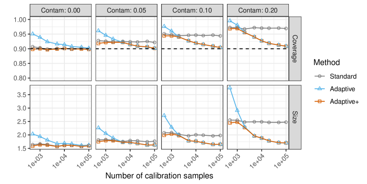
Figure 2: Performances of different conformal methods on simulated data with random label contamination of varying strength, as a function of the number of calibration samples. The dashed horizontal line indicates the 90% nominal label-conditional coverage level.

Figure 2 compares the performances of the prediction sets obtained with the three alternative methods, measured in terms empirical coverage—the average proportion of test points for which the true label is contained in the prediction set—and average size. The results are shown as a function of the number of calibration data points and of the contamination parameter $\epsilon$, averaging over 25 independent repetitions of each experiment. Unsurprisingly, the sets produced by the standard conformal inference approach are overly conservative if $\epsilon>0$ and their size does not change significantly as the number of calibration samples increases. By contrast, the Adaptive and Adaptive+ methods tend to produce more informative prediction sets as the calibration sample grows. Further, the Adaptive+ sets can be smaller than both the standard and Adaptive sets, as long as the number of calibration samples is large enough. Overall, these experiments demonstrate that our Adaptive and Adaptive+ methods are effective at constructing more informative prediction sets with valid coverage in the presence of label contamination, and that the optimistic Adaptive+ version is preferable in practice, even though its theoretical guarantee relies on slightly stronger technical assumptions on the coverage inflation factor (ref. Section 3.1.4).

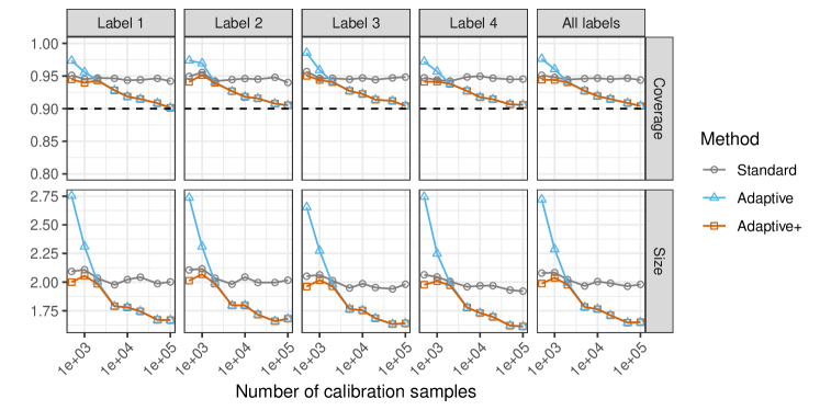
Figure A1: Performances of different conformal methods on simulated data with randomly contaminated labels, as a function of the number of calibration samples. The reported empirical coverage and average size of the prediction sets are stratified based on the true label of the test points. The strength parameter of the label contamination process is $\epsilon=0.1$. Other details are as in Figure 2.

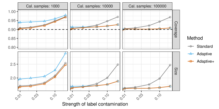
Figure A2: Performances of different conformal methods on simulated data with varying numbers of calibration samples, as a function of the label contamination strength. Other details are as in Figure 2.

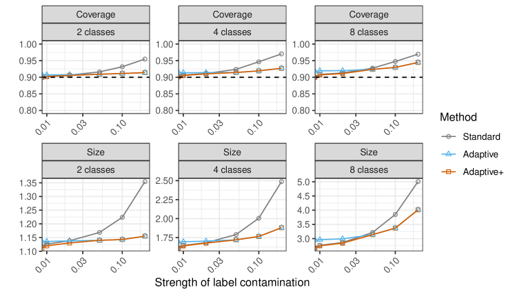
Figure A3: Performances of different conformal methods on simulated classification data with different numbers of labels, as a function of the contamination strength. The strength parameter of the label contamination process is $\epsilon=0.1$. Other details are as in Figure A2.

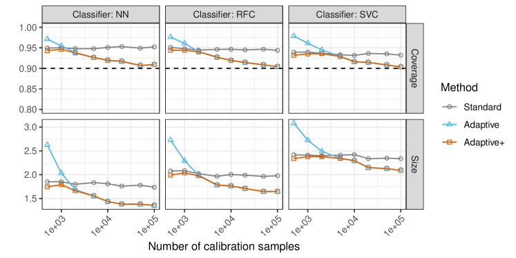
Figure A4: Performances of different conformal methods on simulated data using different machine learning classifiers, as a function of the number of calibration samples. The strength parameter of the label contamination process is $\epsilon=0.1$. Other details are as in Figure 2.

Additional numerical results. Figures A1–A13 in Appendix A4.1 present the results of further experiments with similar conclusions. Figure A1 reports additional performance metrics from the experiments of Figure 2, stratifying the results based on the true label of the test point. This confirms that all methods under comparison achieve 90% label-conditional coverage. Figure A2 gives an alternative view of these experiments, by plotting the results as a function of $\epsilon$ separately for different calibration sample sizes. Figure A3 presents results from experiments analogous to those in Figure A2, but fixing $\epsilon=0.1$ and varying instead the number of labels $K$. Figure A4 presents additional results from experiments analogous to those in Figure 2, fixing $\epsilon=0.1$ but utilizing different types of classifiers implemented by the Scikit-Learn package, namely a support vector machine and a neural network.

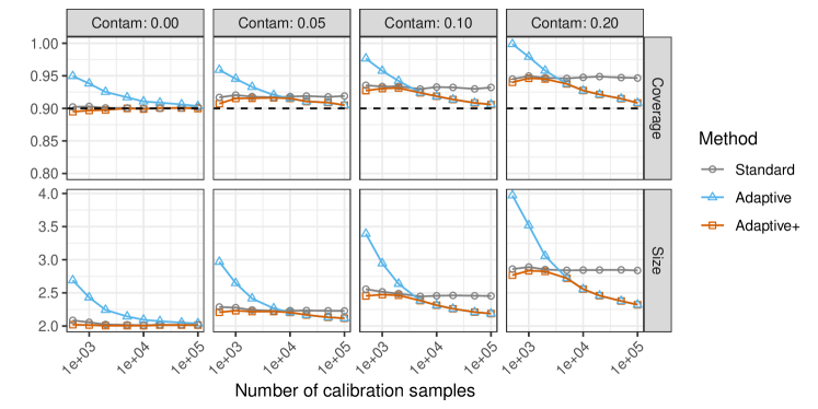
Figure A6: Performances of different conformal methods on simulated data with random label contamination of varying strength, as a function of the number of calibration samples. The data are simulated from a heteroscedastic decision-tree model. Other details are as in Figure 2.

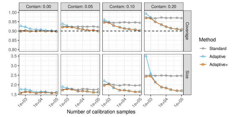
Figure A10: Performances of different conformal prediction methods with marginal coverage on simulated data with random label contamination of varying strength, as a function of the number of calibration samples. The dashed horizontal line indicates the 90% nominal marginal coverage level. Other details are as in Figure 2.

The effect of the data distribution. The robustness of our results to different data distributions is demonstrated by Figures A5 and A6, which report on experiments similar to those of Figure A10. In particular, the experiments of Figure A5 are conducted using data with $K=4$ classes simulated from a logistic model with random parameters, inspired by [38, 17], which can described as follows. The features follow a standard multivariate Gaussian distribution of dimensions $d=50$, and the conditional distribution of $Y\mid X$ is multinomial with weights proportional to $\exp[(X^{T}W)_{k})]$, for all $k\in[K]$, where $W\in\mathbb{R}^{d\times K}$ is an independent standard normal random vector. The experiments of Figure A6 also involve synthetic data with $K=4$ classes, but those data are generated from the heteroscedastic decision-tree model defined in Appendix A5.1, which is borrowed from [38].

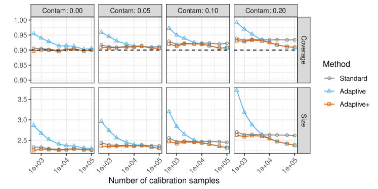
Figure A7: Performances of different conformal methods on simulated data with random label contamination of varying strength, as a function of the number of calibration samples. The contamination process has a block-like structure that preserves the label frequencies. Other details are as in Figure A5.

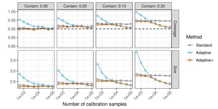
Figure A8: Performances of different conformal methods on simulated data with random label contamination of varying strength, as a function of the number of calibration samples. The label contamination process has a random heterogeneous structure that preserves the label frequencies. Other details are as in Figure A5.

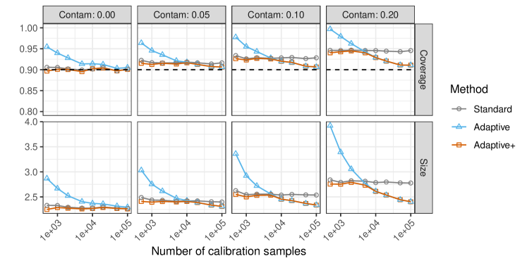
Figure A9: Performances of different conformal methods on simulated data with random label contamination of varying strength, as a function of the number of calibration samples. The label contamination process has a random heterogeneous structure that tends to over-represent more common labels. Other details are as in Figure A5.

The effect of the label contamination process. The robustness of our results to different data distributions is demonstrated by Figures A7–A9, which report on experiments based on synthetic data generated from a logistic model with random parameters, as in Figure A5. However, the difference is that now the labels are contaminated differently. In the experiments of Figure A7, the contamination process has a block-like structure that preserves the label frequencies. That is, $\tilde{\rho}_{k}=\rho_{k}$ for all $k\in[K]$, and $M=(1-\epsilon)I+\epsilon/K\cdot B_{K,2}$, where $B_{K,2}$ is a block-diagonal matrix with $K/2$ constant blocks equal to $J_{2}$—the $2\times 2$ matrix of ones. In the experiments of Figures A8 and A9, the contamination model matrix is $M=(1-\epsilon)I+\epsilon/K\cdot U_{K}$, where $U_{K}$ is a matrix of i.i.d. uniform random numbers on $[0,1]$, standardized to have all column sums equal to one. In Figure A8, the contamination process preserves the label frequencies (i.e., $\tilde{\rho}_{k}=\rho_{k}$ for all $k\in[K]$), while in Figure A9 it tends to over-represent more common labels (i.e., $\tilde{\rho}_{k}\propto\rho^{2}_{k}$ for all $k\in[K]$).

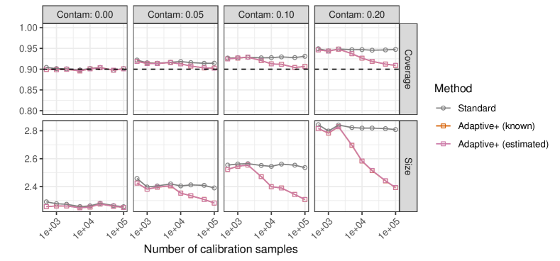
Figure A12: Performances of different conformal methods on simulated data with label contamination. The label contamination process is homogeneous and preserves the label frequencies. The Adaptive+ method is applied with and without perfect knowledge of the label frequencies. Note that there is no significant difference in performance here, because $\tilde{\rho}=\rho$, which makes the estimation problem very easy. The nominal marginal coverage level is 90%. Other details are as in Figure A5.

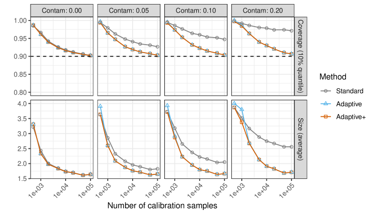
Figure A14: Performances of different conformal methods on simulated data with random label contamination of varying strength, as a function of the number of calibration samples. All methods guarantee 90% calibration and label-conditional coverage with probability at least 90% over the calibration data. Other details are as in Figure A10.

Prediction sets targeting other notions of coverage. Figures A10 and A11 present results from experiments analogous to those described in Figures 2 and A2, respectively, with the only difference that all methods under comparison are applied to seek 90% marginal coverage instead of 90% label-conditional coverage. Within our adaptive framework, this is obtained by replacing Algorithm 1 with Algorithm 2, as explained in Section 4.1. Then, Figures A12 and A13 demonstrate the robustness of Algorithm 2 to the empirical estimation of the label frequencies $\tilde{\rho}$ and $\rho$ from the available contaminated data. Finally, Figure A14 reports on experiments in which the goal is to achieve valid coverage conditional on the calibration data. Within our adaptive framework, this is obtained by replacing Algorithm 1 with Algorithm 3, as explained in Section 4.2.

5.2 Simulations under bounded label contamination

In this section, we present the results of numerical experiments designed to investigate the empirical performance of Algorithm 6 from Section 3.3, which does not require perfect knowledge of the contamination model matrix $M$. In particular, we now assume that $M$ can be characterized by a single contamination strength parameter $\epsilon$ as in (23), and we imagine that some confidence bounds are available for $\epsilon$.

Figure 3 compares the performance of Algorithm 6 (Adaptive) and its optimistic variation (Adaptive+), described in Section 3.3, to that of the standard conformal method that ignores label contamination, using synthetic data sets similar to those utilized for the experiments of Figure 2. The main differences are that now the number of possible labels is varied, $K\in\{2,4,8\}$, the number of calibration samples is fixed to 10,000, and the true contamination parameter is also fixed to $\epsilon=0.2$. The Adaptive (and Adaptive+) prediction sets are constructed by applying Algorithm 6 (and its optimistic variation) based on a given 99% confidence interval for $\epsilon$ whose lower bound is varied as a control parameter, while the upper bound is fixed to $0.2$. The results show that our prediction sets always achieve valid label-conditional coverage and become increasingly informative as the available lower confidence bound for $\epsilon$ increases, as anticipated by the theory in Section 3.3.

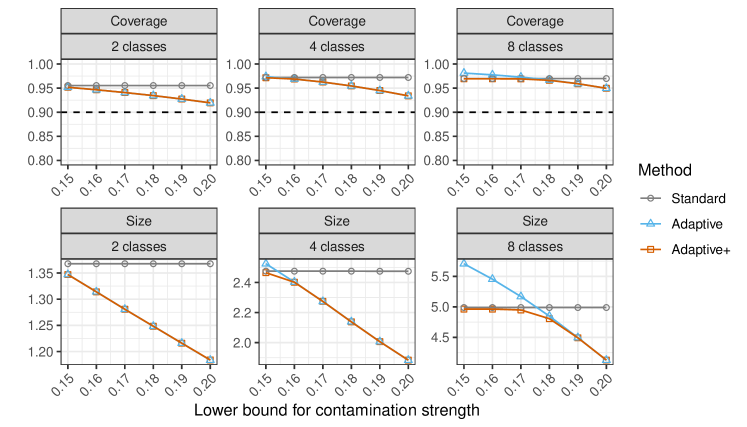
Figure 3: Performances of different conformal methods on simulated data with random label contamination, as a function of the known lower bound for the true contamination strength $\epsilon=0.2$. The results are stratified based on the numbers of possible labels in the data. The number of calibration samples is 10,000. Other details are as in Figure 2.

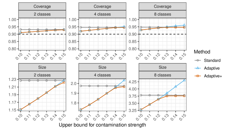
Figure A15: Performances of different conformal methods on simulated data with random label contamination, as a function of the known upper confidence bound for the contamination strength parameter $\epsilon=0.1$. Other details are as in Figure 3.

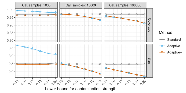
Figure A16: Performances of different conformal methods on simulated data with random label contamination, as a function of the known lower confidence bound for the contamination strength parameter $\epsilon=0.2$. The results are stratified based on the numbers of calibration samples. Other details are as in Figure 3.

Additional results from related experiments, with qualitatively similar conclusions, are presented by Figures A15–A17 in Section A4.2. Figure A15 reports on experiments that differ from those in Figure 3 in that the upper bound for the contamination strength is varied as a control parameter while the lower bound is fixed equal to the true value of $\epsilon$. Figures A16 and A17 report on the results of experiments similar to those of Figure 3, respectively fixing the true contamination parameter equal to $\epsilon=0.2$ and $\epsilon=0.1$, while varying the corresponding lower confidence bound as well as the size of the calibration sample. Overall, these results confirm that tighter confidence bounds for $\epsilon$ generally allow Algorithm 6 to construct more informative prediction sets, and that the practical advantage of our adaptive method is enhanced when the contaminated calibration data set is large.

5.3 Simulations with estimated contamination strength

In this section, we study the empirical performance of the methods described in Section 3.4 for estimating the unknown contamination parameter $\epsilon$ using an independent “model-fitting” data set containing both clean and contaminated labels. In particular, we compare the performance of three alternative implementations of our Adaptive+ method to the standard conformal approach in experiments based on synthetic data similar to those utilized for Figure 3, with $K=2$ possible labels. The first implementation of our method, namely Adaptive+, consists of applying the optimistic version of Algorithm 1 using perfect oracle knowledge of the true contamination model matrix $M$ in (23), based on the correct parameter value $\epsilon=0.2$; this corresponds to the method previously investigated in the experiments of Section 5.1. The second implementation of our method, which we call Adaptive+ (plug-in), consists of applying the optimistic version of Algorithm 1 using an approximate version of $M$ obtained by replacing the unknown parameter $\epsilon$ in (23) with an intuitive point estimate $\hat{\epsilon}$ calculated from the model-fitting data as explained in Section 3.4. The third implementation of our method, which we call Adaptive+ (CI), consists of applying the optimistic version of Algorithm 6 using a 99% bootstrap confidence interval for $\epsilon$, which we compute from the model-fitting data, as also explained in Section 3.4. For simplicity, Algorithm 6 is applied assuming a known fixed upper bound for $\epsilon=0.2$ equal to $\bar{\varepsilon}=0.2$, so that the bootstrap is effectively only needed to estimate the lower confidence bound.

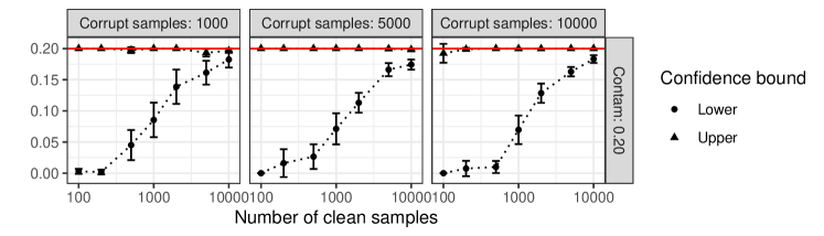
Figure A18: Bootstrap confidence intervals, for the label contamination strength parameter $\epsilon$, utilized by the Adaptive+ (CI) method in Figure 4.

Figure 4 reports on the performance of all aforementioned methods as a function of the size and composition of the model-fitting data set. The results show that the heuristic Adaptive+ (plug-in) method performs very similarly to the ideal Adaptive+ method based on oracle knowledge of the true contamination parameter $\epsilon$. By contrast, the Adaptive+ (CI) tends to be more conservative and can lead to prediction sets that are significantly more informative compared to the standard conformal inference benchmark only if the number of clean samples in the model-fitting data set is sufficiently large. Figure A18 in Section A4.3 plots explicitly the average upper and lower bounds of the bootstrap confidence intervals estimated by the Adaptive+ (CI) in the experiments of Figure 4.

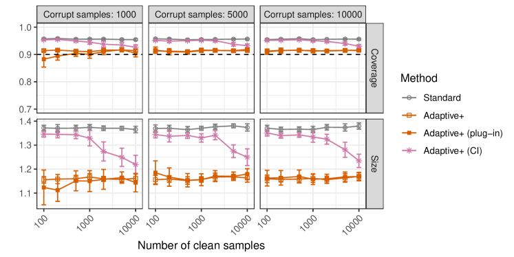
Figure 4: Performances of different conformal prediction methods, as a function of the numbers of clean and corrupt samples used to fit the label contamination model. The number of possible classes is $K=2$. Other details are as in Figure 3.

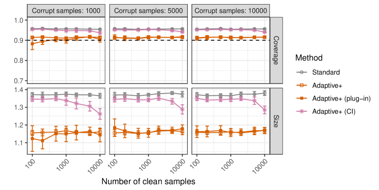
Figure A19: Performances of different conformal prediction methods, as a function of the numbers of clean and corrupt samples used to fit the label contamination model. The fixed upper bound for $\epsilon=0.2$ utilized by the Adaptive+ (CI) method, namely Algorithm 6, is equal to $\bar{\varepsilon}=0.25$. Other details are as in Figure 4.

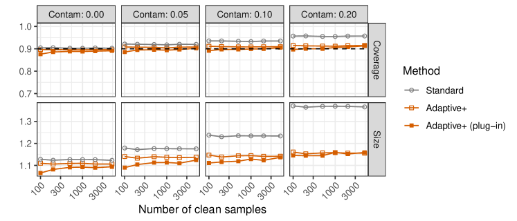
Figure A21: Performances of different conformal methods on simulated data with random label contamination, as a function of the number of clean samples used to fit the contamination model. The results are stratified based on the true contamination parameter $\epsilon$. Other details are as in Figure 4.

Additional results from related experiments, with qualitatively similar conclusions, are presented by Figures A19–A23 in Section A4.3. In particular, Figures A19 and A20 report on results analogous to those in Figures 4 and A18, respectively, with the only difference that now the fixed upper bound for $\epsilon=0.2$ utilized by the Adaptive+ (CI) method is set equal to $\bar{\varepsilon}=0.25$. Figures A21–A23 further demonstrate the power and robustness of the Adaptive+ (plug-in) method in experiments with different values of the true contamination parameter $\epsilon$ and different numbers of possible labels.

5.4 Robustness to model mis-specification

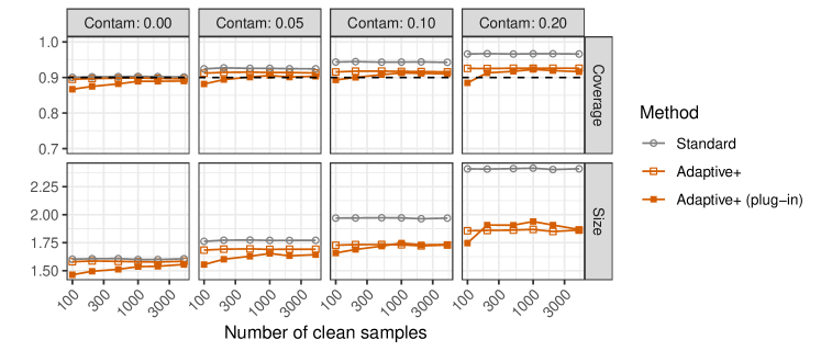
Figure A24: Performances of different conformal methods on simulated data, as a function of the number of clean samples used to estimate a mis-specified contamination model. The contamination model matrix $M$ has a random structure. Other details are as in Figure 5.

This section demonstrates the robustness of our adaptive methods to other types of mis-specifications in the label contamination model, going beyond the issue of estimating the parameter $\epsilon$ in (23). For this purpose, we generate synthetic data with $K=4$ possible labels as explained in Section 5.1, but using a label contamination process with a block-like structure that preserves the label frequencies. That is, $\tilde{\rho}_{k}=\rho_{k}$ for all $k\in[K]$, and $M=(1-\epsilon)I+\epsilon/K\cdot B_{K,2}$, where $B_{K,2}$ is a block-diagonal matrix with $K/2$ constant blocks equal to $J_{2}$—the $2\times 2$ matrix of ones. Then, we apply the optimistic version of Algorithm 1 under the incorrect assumption that $M=(1-\epsilon)I+\epsilon/K\cdot J_{K}$, separately using either the correct value of $\epsilon$ or a plug-in empirical estimate obtained from an independent model-fitting data set as in Section 5.3. Consistently with the previous section, we refer to the former method as Adaptive+ and to the latter as Adaptive+ (plug-in). Figure 5 compares the performances of our Adaptive+ and Adaptive+ (plug-in) to that of the standard conformal inference approach, as a function of the true $\epsilon$ and of the number of clean model-fitting data points used to estimate this parameter. The number of calibration data points here is set equal to 10,000. The results show that both methods are quite robust to model mis-specification and can generally produce more informative prediction sets compared to the standard benchmark. Finally, Figure A24 in Section A4.4 demonstrates that our methods also enjoy similar robustness under different label contamination processes, focusing specifically on $M=(1-\epsilon)I+\epsilon/K\cdot U_{K}$, where $U_{K}$ is a matrix of i.i.d. uniform random numbers on $[0,1]$, standardized to have all column sums equal to one.

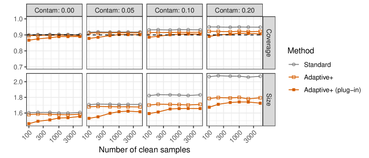
Figure 5: Performances of different conformal methods on simulated data, as a function of the number of clean samples used to estimate a mis-specified contamination model. The true model matrix $M$ has a block-diagonal structure, and the results are stratified based on the contamination strength. Other details are as in Figure 2.

5.5 Demonstrations with CIFAR-10 image data

This section provides a demonstration of our methods in a object classification application based on real-world 32x32 color images. As anticipated in Section 1, we focus on the CIFAR-10H data set [23], a variation of the larger CIFAR-10 data set [48] that includes imperfect labels assigned by approximately 50 independent human annotators via the Amazon Mechanical Turk, for a subset of 10,000 images. Each image depicts an object belonging to one of 10 possible classes: airplane, car, bird, cat, deer, dog, frog, horse, ship, or truck. Since the individual annotators do not always agree on the content of each image, we can think of their labels as being a randomly contaminated version of the corresponding “true” labels contained in the original CIFAR-10 data set. Our goal is to construct informative prediction sets for the true labels, using a conformal predictor calibrated on the contaminated data. For simplicity, we work with a slightly modified version of the CIFAR-10H data in which each image has a single corrupt label $\tilde{Y}$, randomly sampled from a multinomial distribution whose weights are equal to the relative label frequencies assigned to that image by different human annotators. Note that these corrupted labels coincide with the true CIFAR-10 labels approximately 95.4% of the time; see Figure 6 (a) for a visualization of some images for which the labels do not match.

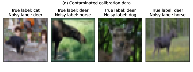
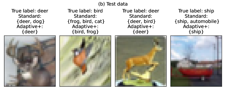
Figure 6: Demonstration of some CIFAR-10 images with contaminated labels (a), and of conformal prediction sets (b) obtained with and without correcting for the presence of label contamination in the calibration data, as in the experiments of Figure 1.

A ResNet-18 convolutional neural network serves as base classifier; this is implemented by the PyTorch Python package [49] and was pre-trained using the 50,000 CIFAR-10 images excluded from the CIFAR-10H data set. The output of the final soft-max layer of the deep neural network provides estimates of the class probabilities for any new given image, and from that we calculate conformity scores with the recipe reviewed in Section A1.1. The conformal predictor is then calibrated using three alternative methods, based on a random subset of the 10,000 CIFAR-10H images whose size is varied as a control parameter.

The first method considered is Algorithm 5, the standard conformal inference approach that seeks marginal coverage while ignoring label contamination. The second method (Adaptive+) is the optimistic variation of Algorithm 2 from Section 4.1, which we apply assuming that $\rho_{k}=\tilde{\rho}_{k}$ for all $k\in[K]$ and using the contamination model matrix $M$ given by (23) with $\epsilon=0.051$. This value of $\epsilon$ was chosen to match the average proportion of CIFAR-10H samples for which $Y\neq\tilde{Y}$, which is approximately $0.046$. The third method (Adaptive+ (plug-in)) differs from the Adaptive+ method in that it utilizes a plug-in estimate of $\epsilon$ obtained with the same maximum-likelihood approach previously demonstrated in Section 5.4. This estimate of $\epsilon$ is evaluated as explained in Section 3.4, by applying the same pre-trained ResNet-18 convolutional neural network to a smaller independent data set containing both clean and corrupted data in equal proportions. In particular, the number of clean images used to estimate $\epsilon$ is 10% of the total number of corrupt images in the calibration set.

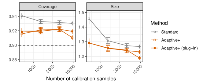
Figure A25: Performances of different conformal methods for label-conditional coverage on CIFAR-10 image data with noisy human-assigned labels, as a function of the number of calibration samples. The horizontal dashed line indicates the nominal 90% label-conditional coverage level. Other details are as in Figure 1.

Figure 1, previewed in Section 1.2, reports on the prediction sets constructed by the three aforementioned methods for a random test set 500 CIFAR-10H images, varying the size of the calibration sample between 500 and 9500. All experiments are independently repeated 50 times, using different random splits of the CIFAR-10H data into calibration, model-fitting, and test subsets. The results show that the standard conformal inferences are overly conservative, while our adaptive approaches are able to achieve valid coverage with increasingly more informative prediction sets as the size of the calibration sample increases. See Figure 6 (b) for a visualization of some concrete examples in which our Adaptive+ method leads to more informative prediction sets compared to the standard conformal inference benchmark. Finally, Figure A25 in Section A4.5 presents analogous results from similar experiments in which we target label-conditional coverage instead of marginal coverage, using Algorithms 1 and 4 instead of Algorithms 2 and 5, respectively.

6 Discussion

This paper began by studying the behavior of standard conformal classification methods in the presence of calibration data with contaminated labels, highlighting how the prediction sets may become either overly liberal or, more typically, too conservative. Then, it developed a novel conformal inference method that can automatically adapt to label contamination, producing prediction sets that enjoy more robust coverage guarantees and are often more informative compared to those given by state-of-the-art approaches. Several variations of our method were presented, enabling control of different coverage metrics and allowing one to leverage different levels of knowledge about the label contamination process. The theoretical and empirical results have shown that the advantages of our methods are more pronounced when applied with larger contaminated calibration samples. This makes our work especially relevant to real-world applications in which there is an abundance of relatively low-quality data but accurate labels are expensive to collect.

This research opens several opportunities for future work. For example, it may be interesting to study possible extensions of our methods that can be applied with regression data, or even with other types of more complex data for which conformal inference has already been utilized, including causal inference [50, 51], survival analysis [52], data sketching [42, 53], and matrix completion [54]. Alternatively, it may be possible to build upon our work to account for label contamination in the context of more sophisticated conformal prediction frameworks such as full-conformal inference [1] and cross-validation+ [55], which are more computationally expensive but can make more efficient use of limited observations.

Supporting code is available at https://github.com/msesia/conformal-label-noise.

Appendix A1 Review of standard conformal classification methods

A1.1 Conformity scores based on generalized inverse quantiles

We briefly review here the construction of the generalized inverse quantile conformity scores proposed by [38], upon which we rely in the empirical demonstrations of Section 5. These conformity scores are more involved compared to the classical homogeneous scores defined in (2), but they have the advantage of leading to more flexible prediction sets that can account for possible heteroscedasticity in the distribution of $Y\mid X$. We refer to [38] or [37] for further information about the limitations of the scores in (2).

For any $x\in\mathbb{R}^{d}$ and $t\in[0,1]$, define

$$\hat{Q}(x,\hat{\pi},t) =\min\{k\in\{1,\ldots,K\}:\hat{\pi}_{(1)}(x)+\hat{\pi}_{(2)}(x)+\ldots+\hat{\pi}_{(k)}(x)\geq t\},$$ (A48)

where $\hat{\pi}_{(1)}(x)\geq\ldots\geq\hat{\pi}_{(K)}(x)$ are the descending order statistics of $\hat{\pi}(x,1),\ldots,\hat{\pi}(x,K)$. Intuitively, $\hat{Q}(x,\hat{\pi},\cdot)$ may be seen as a generalized quantile function. Similarly, let $\hat{r}(x,\hat{\pi},k)$ denote the rank of $\hat{\pi}(x,k)$ among $\hat{\pi}(x,1),\ldots,\hat{\pi}(x,K)$. With this notation, one can also define a corresponding generalized cumulative distribution function:

$$\hat{\Pi}(x,\hat{\pi},k)=\hat{\pi}_{(1)}(x)+\hat{\pi}_{(2)}(x)+\ldots+\hat{\pi}_{(\hat{r}(x,\hat{\pi},k))}(x).$$

Then, the function $\mathcal{C}$ proposed by [38] can be written as:

$$\mathcal{C}(x;\hat{\pi},\tau) =\{k\in[K]:\hat{r}(x,\hat{\pi},k)\leq\hat{Q}(x,\hat{\pi},\tau_{k})\},$$ (A49)

and the corresponding conformity scores defined in (1) can be evaluated efficiently by noting that $\hat{s}(X_{i},k)=\hat{\Pi}(x,k)$; see [38] for further details.

The prediction function defined in (A49) may be understood by noting that, if $\tau=(\tau_{0},\ldots,\tau_{0})$ for some $\tau_{0}\in[0,1]$, the output of $\mathcal{C}(x;\hat{\pi},\tau)$ is the list of most likely classes according to $\hat{\pi}(x)$ up until the first label $l$ for which $\hat{\Pi}(x,\hat{\pi},l)\geq\tau_{0}$. Therefore, in the ideal case where $\hat{\pi}(x,k)=\mathbb{P}\left[Y=k\mid X=x\right]$, one can verify that $\mathcal{C}(x;\hat{\pi},\tau)$ is the smallest possible (deterministic) prediction set for $Y$ with perfect object-conditional coverage at level $\tau_{0}$, i.e., satisfying $\mathbb{P}\left[Y\in\mathcal{C}(x;\hat{\pi},\tau)\mid X=x\right]\geq\tau_{0}$ [38]. Note that [38] also developed a more powerful randomized version of (A49) that enjoys similar theoretical properties while being able to produce even more informative prediction sets. The results of this paper can also seamlessly accommodate such additional randomness in $\mathcal{C}$, and indeed that is the practical approach followed in the empirical demonstrations of Section 5, but we choose not to review such extension explicitly here to avoid making the notation too cumbersome.

A1.2 Prediction sets with label-conditional coverage

1

Input: Data set $\{(X_{i},\tilde{Y}_{i})\}_{i=1}^{n}$, with observable labels $\tilde{Y}_{i}\in[K]$.

         Unlabeled test point with features $X_{n+1}$.

         Machine learning algorithm $\mathcal{A}$ for training a $K$-class classifier.

         A valid prediction function $\mathcal{C}$ satisfying Definition 1; e.g., (2).

         Desired coverage parameter $\alpha$.

2

3Randomly split $[n]$ into two disjoint subsets, $\mathcal{D}^{\text{train}}$ and $\mathcal{D}^{\mathrm{cal}}$.

4 Train the classifier $\mathcal{A}$ on the data in $\mathcal{D}^{\text{train}}$.

5 for $k=1,\dots,K$ do

6       Define $\mathcal{D}_{k}^{\mathrm{cal}}=\{i\in\mathcal{D}^{\mathrm{cal}}:Y_{i}=k\}$ and $n_{k}=|\mathcal{D}_{k}^{\mathrm{cal}}|$.

7       Compute $\hat{s}(X_{i},k)$ using (1), for all $i\in\mathcal{D}_{k}^{\mathrm{cal}}$.

8       Sort the scores $\{s(X_{i},k):i\in\mathcal{D}_{k}^{\mathrm{cal}}\}$ into $(S^{k}_{(1)},S^{k}_{(2)},\dots,S^{k}_{(n_{k})})$.

9       Define $\hat{i}(k)$ as the $\lceil(1+n_{k})\cdot(1-\alpha)\rceil$ smallest value in $\{\hat{s}(X_{i},k)\}_{i\in\mathcal{D}_{k}^{\mathrm{cal}}}$.

10       Define $\hat{\tau}_{k}=S^{k}_{(\hat{i}(k))}$.

11      

12 end for

13Evaluate $\hat{C}(X_{n+1})=\mathcal{C}(X_{n+1},\hat{\tau};\hat{\pi})$, where $\hat{\tau}=(\hat{\tau}_{1},\ldots,\hat{\tau}_{K})$.

Output: Conformal prediction set $\hat{C}(X_{n+1})$ for $Y_{n+1}$, satisfying (4).

14

Algorithm 4 Standard conformal classification with label-conditional coverage.

Proposition A1 (e.g., from [18] or [38]).

If the data pairs $(X_{i},\tilde{Y}_{i})$, for all $i\in[n+1]$, are exchangeable random samples from some joint distribution, the prediction set $\hat{C}(X_{n+1})$ output by Algorithm 4 has label-conditional coverage (4) for the observable labels $\tilde{Y}$; i.e.,

$$\mathbb{P}\left[\tilde{Y}_{n+1}\in\hat{C}(X_{n+1})\mid\tilde{Y}_{n+1}=k\right]\geq 1-\alpha,\qquad\text{ for all }k\in[K].$$

Further, if all scores $s(X_{i},\tilde{Y}_{i})$ computed by Algorithm 4 are almost-surely distinct,

$$\mathbb{P}\left[\tilde{Y}_{n+1}\in\hat{C}(X_{n+1})\mid\tilde{Y}_{n+1}=k\right]\leq 1-\alpha+\frac{1}{n_{k}+1},\qquad\text{ for all }k\in[K],$$

where $n_{k}=|\mathcal{D}_{k}^{\mathrm{cal}}|$ is the number of data points with label $k$ in the calibration set.

In words, this result tells us that Algorithm 4 is always guaranteed to achieve valid label-conditional coverage for the observable labels $\tilde{Y}$, regardless of which prediction function $\mathcal{C}$ is employed. Note that in the standard setting without label contamination, the observable labels $\tilde{Y}$ are simply assumed to be always equal to $Y$.

A1.3 Prediction sets with marginal coverage

1

Input: Data set $\{(X_{i},\tilde{Y}_{i})\}_{i=1}^{n}$ with observable labels $\tilde{Y}_{i}\in[K]$.

         Unlabeled test point with features $X_{n+1}$.

         Machine learning algorithm $\mathcal{A}$ for training a $K$-class classifier.

         A valid prediction function $\mathcal{C}$ satisfying Definition 1; e.g., (2).

         Desired coverage parameter $\alpha$.

2

3Randomly split $[n]$ into two disjoint subsets, $\mathcal{D}^{\text{train}}$ and $\mathcal{D}^{\mathrm{cal}}$, defining $n_{\mathrm{cal}}=|\mathcal{D}^{\mathrm{cal}}|$.

4 Train the classifier $\mathcal{A}$ on the data in $\mathcal{D}^{\text{train}}$.

5 Compute $\hat{s}(X_{i},\tilde{Y}_{i})$ using (1), for all $i\in\mathcal{D}^{\mathrm{cal}}$.

6 Sort the scores $\{s(X_{i},\tilde{Y}_{i}):i\in\mathcal{D}^{\mathrm{cal}}\}$ into $(S_{(1)},S_{(2)},\dots,S_{(n_{\mathrm{cal}})})$.

7 Define $\hat{i}$ as the $\lceil(1+n_{\mathrm{cal}})\cdot(1-\alpha)\rceil$ smallest value in $\{\hat{s}(X_{i},\tilde{Y}_{i})\}_{i\in\mathcal{D}^{\mathrm{cal}}}$.

8 Define $\hat{\tau}=S_{(\hat{i})}$.

9 Evaluate $\hat{C}(X_{n+1})=\mathcal{C}(X_{n+1},\hat{\tau};\hat{\pi})$, where $\hat{\tau}=(\hat{\tau}_{0},\ldots,\hat{\tau}_{0})$.

Output: Conformal prediction set $\hat{C}(X_{n+1})$ for $\tilde{Y}_{n+1}$, satisfying (5).

10

Algorithm 5 Standard conformal classification with marginal coverage.

Proposition A2 (e.g., from [24] or [38]).

If the data pairs $(X_{i},\tilde{Y}_{i})$, for all $i\in[n+1]$, are exchangeable random samples from some joint distribution, the prediction set $\hat{C}(X_{n+1})$ output by Algorithm 4 has marginal coverage (5) for the observable labels $\tilde{Y}$; i.e.,

$$\mathbb{P}\left[\tilde{Y}_{n+1}\in\hat{C}(X_{n+1})\right]\geq 1-\alpha.$$

Further, if all scores $s(X_{i},\tilde{Y}_{i})$ computed by Algorithm 4 are almost-surely distinct,

$$\mathbb{P}\left[\tilde{Y}_{n+1}\in\hat{C}(X_{n+1})\right]\leq 1-\alpha+\frac{1}{n_{\mathrm{cal}}+1},$$

where $n_{\mathrm{cal}}=|\mathcal{D}^{\mathrm{cal}}|$ is the number of data points in the calibration set.

Appendix A2 Additional methodological details

A2.1 Adaptive coverage under bounded label noise

1

Input: Data set $\{(X_{i},\tilde{Y}_{i})\}_{i=1}^{n}$ with corrupted labels $\tilde{Y}_{i}\in[K]$.

         An independent $1-\alpha_{\xi}$ confidence interval $[\hat{\xi}^{\mathrm{low}},\hat{\xi}^{\mathrm{upp}}]$ for $\xi:=\epsilon/(1-\epsilon)$.

         A known constant $\bar{\xi}^{\mathrm{upp}}\in\mathbb{R}$ such that $\max\{\hat{\xi}^{\mathrm{upp}},\xi\}\leq\bar{\xi}^{\mathrm{upp}}$ almost-surely.

         Unlabeled test point with features $X_{n+1}$.

         Machine learning algorithm $\mathcal{A}$ for training a $K$-class classifier.

         A valid prediction function $\mathcal{C}$ satisfying Definition 1; e.g., (2).

         Desired significance level $\alpha\in(0,1)$.

2

3Randomly split $[n]$ into two disjoint subsets, $\mathcal{D}^{\text{train}}$ and $\mathcal{D}^{\mathrm{cal}}$.

4 Train the classifier $\mathcal{A}$ on the data in $\mathcal{D}^{\text{train}}$.

5 Compute conformity scores $\hat{s}(X_{i},k)$ using (1) for all $i\in\mathcal{D}^{\mathrm{cal}}$ and all $k\in[K]$.

6 Define the empirical CDF $\hat{F}_{l}^{k}$ of $\{\hat{s}(X_{i},k):i\in\mathcal{D}_{l}^{\mathrm{cal}}\}$ for all $l\in[K]$, as in (16).

7 for $k=1,\dots,K$ do

8       Define $\mathcal{D}_{k}^{\mathrm{cal}}=\{i\in\mathcal{D}^{\mathrm{cal}}:\tilde{Y}_{i}=k\}$ and $n_{k}=|\mathcal{D}_{k}^{\mathrm{cal}}|$.

9       Sort the scores $\{\hat{s}(X_{i},k):i\in\mathcal{D}_{k}^{\mathrm{cal}}\}$ into $(S^{k}_{(1)},S^{k}_{(2)},\dots,S^{k}_{(n_{k})})$.

10       Compute $\hat{F}_{l}^{k}(S^{k}_{(i)})$ for all $i\in[n_{k}]$ and $l\in[K]$.

11       Compute ${\widehat{\Delta}}_{k}^{\mathrm{ci}}(S^{k}_{(i)})$ for all $i\in[n_{k}]$, as in (27).

12       Compute $\delta^{\mathrm{ci}}(n_{k},n_{*})$ using (28), based on a Monte Carlo estimate of $c(n_{k})$ in (20).

13       Construct the set $\hat{\mathcal{I}}_{k}\subseteq[K]$ as in (18), using ${\widehat{\Delta}}_{k}^{\mathrm{ci}}$ and $\delta^{\mathrm{ci}}$ instead of ${\widehat{\Delta}}_{k}$ and $\delta$.

14       Evaluate $\hat{\tau}_{k}$ based on $\hat{\mathcal{I}}_{k}$ as in (19).

15 end for

16Evaluate $\hat{C}^{\mathrm{ci}}(X_{n+1})=\mathcal{C}(X_{n+1},\hat{\tau};\hat{\pi})$, where $\hat{\tau}=(\hat{\tau}_{1},\ldots,\hat{\tau}_{K})$.

Output: Conformal prediction set $\hat{C}^{\mathrm{ci}}(X_{n+1})$ for $Y_{n+1}$.

Algorithm 6 Adaptive conformal classification under bounded label noise

A2.2 Estimating the proportion of contaminated labels

1

Input: Data set $\mathcal{D}=\{(X_{i},\tilde{Y}_{i})\}_{i=1}^{n}$ with corrupted labels $\tilde{Y}_{i}\in[K]$.

         Independent data set $\mathcal{D}_{1}=\{(X_{i}^{1},\tilde{Y}^{1}_{i})\}_{i=1}^{n_{0}}$ with corrupted labels $\tilde{Y}^{1}_{i}\in[K]$.

         Small clean data set $\mathcal{D}_{0}=\{(X_{i}^{0},Y^{0}_{i})\}_{i=1}^{n_{0}}$ with labels $Y^{0}_{i}\in[K]$.

         Unlabeled test point with features $X_{n+1}$.

         Machine learning algorithm $\mathcal{A}$ for training a $K$-class classifier.

         A valid prediction function $\mathcal{C}$ satisfying Definition 1; e.g., (2).

         Desired significance level $\alpha\in(0,1)$.

         Desired significance level $\alpha_{\xi}\in(0,\alpha)$ for the estimation of $\xi$.

2

3Randomly split the data in $\mathcal{D}_{1}$ into two disjoint subsets, $\mathcal{D}_{1a}$ and $\mathcal{D}_{1b}$.

4 Train the classifier $\mathcal{A}$ on the data in $\mathcal{D}_{1a}$.

5 Evaluate the predictive accuracy of $\mathcal{A}$ to predict $\tilde{Y}$ in $\mathcal{D}_{1b}$ and $Y$ in $\mathcal{D}_{0}$.

6 Construct a $1-\alpha_{\xi}$ confidence interval $[\hat{\xi}^{\mathrm{low}},\hat{\xi}^{\mathrm{upp}}]$ for $\xi:=\epsilon/(1-\epsilon)$ using the parametric bootstrap, as explained in Section 3.4.

Apply Algorithm 6 to construct a conformal prediction set $\hat{C}^{\mathrm{ci}}(X_{n+1})$ for $Y_{n+1}$. Output: Conformal prediction set $\hat{C}^{\mathrm{ci}}(X_{n+1})$ for $Y_{n+1}$.

Algorithm 7 Adaptive conformal classification with label noise estimation

Appendix A3 Mathematical proofs

A3.1 Preliminaries

Proof of Theorem 1.

By definition of the conformity score function in (1), $Y_{n+1}\in\hat{C}(X_{n+1})$ if and only if $\hat{s}(X_{n+1},Y_{n+1})\leq\hat{\tau}_{Y_{n+1}}$. Therefore,

$$\mathbb{P}\left[Y_{n+1}\in\hat{C}(X_{n+1})\mid Y_{n+1}=k\right]$$

$$\qquad=\mathbb{P}\left[\tilde{Y}_{n+1}\in\hat{C}(X_{n+1})\mid\tilde{Y}_{n+1}=k\right]+$$

$$\qquad\qquad\mathbb{P}\left[Y_{n+1}\in\hat{C}(X_{n+1})\mid Y_{n+1}=k\right]-\mathbb{P}\left[\tilde{Y}_{n+1}\in\hat{C}(X_{n+1})\mid\tilde{Y}_{n+1}=k\right],$$

$$\qquad=\mathbb{P}\left[\tilde{Y}_{n+1}\in\hat{C}(X_{n+1})\mid\tilde{Y}_{n+1}=k\right]$$

$$\qquad\qquad+\mathbb{E}\left[\mathbb{P}\left[Y_{n+1}\in\hat{C}(X_{n+1})\mid Y_{n+1}=k,\mathcal{D}\right]-\mathbb{P}\left[\tilde{Y}_{n+1}\in\hat{C}(X_{n+1})\mid\tilde{Y}_{n+1}=k,\mathcal{D}\right]\right]$$

$$\qquad=\mathbb{P}\left[\tilde{Y}_{n+1}\in\hat{C}(X_{n+1})\mid\tilde{Y}_{n+1}=k\right]$$

$$\qquad\qquad+\mathbb{E}\left[\mathbb{P}\left[\hat{s}(X_{n+1},k)\leq\hat{\tau}_{k}\mid Y_{n+1}=k,\mathcal{D}\right]-\mathbb{P}\left[\hat{s}(X_{n+1},k)\leq\hat{\tau}_{k}\mid\tilde{Y}_{n+1}=k,\mathcal{D}\right]\right]$$

$$\qquad=\mathbb{P}\left[\tilde{Y}_{n+1}\in\hat{C}(X_{n+1})\mid\tilde{Y}_{n+1}=k\right]+\mathbb{E}\left[F_{k}^{k}(\hat{\tau}_{k})-\tilde{F}_{k}^{k}(\hat{\tau}_{k})\right]$$

$$\qquad=\mathbb{P}\left[\tilde{Y}_{n+1}\in\hat{C}(X_{n+1})\mid\tilde{Y}_{n+1}=k\right]+\mathbb{E}\left[\Delta_{k}({\widehat{\tau}}_{k})\right].$$

Above, the notation $\mathbb{E}\left[\cdot\mid\mathcal{D}\right]$ indicates the expected value conditional on the training and calibration data sets. From this, Equations (8) and (9) follow directly because

$$1-\alpha\leq\mathbb{P}\left[\tilde{Y}_{n+1}\in\hat{C}(X_{n+1})\mid\tilde{Y}_{n+1}=k\right]\leq 1-\alpha+\frac{1}{n_{k}+1},$$

by Proposition A1, which applies here since the data pairs $(X_{i},\tilde{Y}_{i})$ are i.i.d. random samples. ∎

Proof of Theorem 2.

The proof strategy is similar to that of Theorem 1. By definition of the conformity score function in (1), $Y_{n+1}\in\hat{C}(X_{n+1})$ if and only if $\hat{s}(X_{n+1},Y_{n+1})\leq\hat{\tau}_{Y_{n+1}}$. Therefore,

$$\mathbb{P}\left[Y_{n+1}\in\hat{C}(X_{n+1})\right]$$

$$\qquad=\mathbb{P}\left[\tilde{Y}_{n+1}\in\hat{C}(X_{n+1})\right]+\left(\mathbb{P}\left[Y_{n+1}\in\hat{C}(X_{n+1})\right]-\mathbb{P}\left[\tilde{Y}_{n+1}\in\hat{C}(X_{n+1})\right]\right).$$

The proof is then completed by noting that the second term on the right-hand-side above can be written as:

$$\mathbb{P}\left[Y_{n+1}\in\hat{C}(X_{n+1})\right]-\mathbb{P}\left[\tilde{Y}_{n+1}\in\hat{C}(X_{n+1})\right]$$

$$\qquad=\sum_{k=1}^{K}\left(\rho_{k}\cdot\mathbb{P}\left[Y_{n+1}\in\hat{C}(X_{n+1})\mid Y_{n+1}=k\right]-\tilde{\rho}_{k}\cdot\mathbb{P}\left[\tilde{Y}_{n+1}\in\hat{C}(X_{n+1})\mid\tilde{Y}_{n+1}=k\right]\right)$$

$$\qquad=\sum_{k=1}^{K}\left(\rho_{k}\cdot\mathbb{P}\left[\hat{s}(X_{n+1},k)\leq\hat{\tau}\mid Y_{n+1}=k\right]-\tilde{\rho}_{k}\cdot\mathbb{P}\left[\hat{s}(X_{n+1},k)\leq\hat{\tau}\mid\tilde{Y}_{n+1}=k\right]\right)$$

$$\qquad=\mathbb{E}\left[\sum_{k=1}^{K}\left[\rho_{k}F_{k}^{k}(\hat{\tau})-\tilde{\rho}_{k}\tilde{F}_{k}^{k}(\hat{\tau})\right]\right]$$

$$\qquad=\mathbb{E}\left[\Delta(\hat{\tau})\right].$$

∎

Proof of Proposition 1.

$$\tilde{P}_{k} =\mathbb{P}\left[X\mid\tilde{Y}=k\right]$$

$$=\sum_{l=1}^{K}\mathbb{P}\left[X,Y=l\mid\tilde{Y}=k\right]$$

$$=\sum_{l=1}^{K}\frac{\mathbb{P}\left[X,\tilde{Y}=k\mid Y=l\right]\cdot\mathbb{P}\left[Y=l\right]}{\mathbb{P}\left[\tilde{Y}=k\right]}$$

$$=\sum_{l=1}^{K}\frac{\mathbb{P}\left[X\mid Y=l\right]\cdot\mathbb{P}\left[\tilde{Y}=k\mid Y=l\right]\cdot\mathbb{P}\left[Y=l\right]}{\mathbb{P}\left[\tilde{Y}=k\right]}$$

$$=\sum_{l=1}^{K}P(X\mid Y=l)\cdot\mathbb{P}\left[Y=l\mid\tilde{Y}=k\right]$$

$$=\sum_{l=1}^{K}P_{l}\cdot M_{kl}.$$

Above, the fourth equality follows directly from 1. ∎

Proof of Corollary 1.

By Theorem 1, it suffices to prove that $\mathbb{E}\left[\Delta_{k}(t)\right]\geq 0$ for all $t\in\mathbb{R}$ and $k\in[K]$. To establish that, note that combining (7) with Proposition 1 gives:

$$\Delta_{k}(t) =F_{k}^{k}(t)-\tilde{F}_{k}^{k}(t)$$

$$=(1-m_{kk})F_{k}^{k}(t)-\sum_{j\neq k}m_{kj}F_{j}^{k}(t)$$

$$\geq(1-m_{kk})F_{k}^{k}(t)-\bigg{(}\sum_{j\neq k}m_{kj}\bigg{)}\cdot\max_{j\neq k}F_{j}^{k}(t).$$

Further, by (14),

$$\Delta_{k}(t) \geq(1-m_{kk})F_{k}^{k}(t)-\bigg{(}\sum_{j\neq k}m_{kj}\bigg{)}\cdot F_{k}^{k}(t)$$

$$=\left(1-\sum_{j=1}^{K}m_{kj}\right)\cdot F_{k}^{k}(t)=0,$$

where the last equality follows from the fact that $\sum_{j=1}^{K}m_{kj}=1$. This implies that $\mathbb{E}\left[\Delta_{k}({\widehat{\tau}}_{k})\right]\geq 0$, completing the proof. ∎

Proof of Corollary 2.

By Theorem 2, it suffices to prove $\mathbb{E}\left[\Delta(t)\right]\geq 0$ for all $t\in\mathbb{R}$. To establish that, note that combining (10) with Proposition 1 gives:

$$\Delta(t) =\sum_{k=1}^{K}\left[\rho_{k}F_{k}^{k}(t)-\tilde{\rho}_{k}\tilde{F}_{k}^{k}(t)\right]$$

$$=\sum_{k=1}^{K}\left\{\rho_{k}F_{k}^{k}(t)-\sum_{l=1}^{K}M_{kl}\tilde{\rho}_{k}F_{l}^{k}(t)\right\}.$$

To simplify the notation in the following, define

$$W_{kl} :=\mathbb{P}[\tilde{Y}=k\mid X,Y=l]$$

$$=M_{kl}\frac{\tilde{\rho}_{k}}{\rho_{l}}.$$

Then,

$$\Delta(t) =\sum_{l=1}^{K}\rho_{l}F_{l}^{l}(t)-\sum_{l=1}^{K}\rho_{l}\sum_{k=1}^{K}W_{kl}F_{l}^{k}(t)$$

$$=\sum_{l=1}^{K}\rho_{l}F_{l}^{l}(t)-\sum_{l=1}^{K}\rho_{l}\left\{W_{ll}F_{l}^{l}(t)+\sum_{k\neq l}W_{kl}F_{l}^{k}(t)\right\}$$

$$\geq\sum_{l=1}^{K}\rho_{l}F_{l}^{l}(t)-\sum_{l=1}^{K}\rho_{l}\left\{W_{ll}F_{l}^{l}(t)+\left(\sum_{k\neq l}W_{kl}\right)\max_{k\neq l}F_{l}^{k}(t)\right\}$$

$$=\sum_{l=1}^{K}\rho_{l}F_{l}^{l}(t)-\sum_{l=1}^{K}\rho_{l}\left\{W_{ll}F_{l}^{l}(t)+\left(\sum_{k=1}^{K}W_{kl}\right)\max_{k\neq l}F_{l}^{k}(t)-W_{ll}\max_{k\neq l}F_{l}^{k}(t)\right\}$$

$$=\sum_{l=1}^{K}\rho_{l}F_{l}^{l}(t)-\sum_{l=1}^{K}\rho_{l}\left\{W_{ll}F_{l}^{l}(t)+\max_{k\neq l}F_{l}^{k}(t)-W_{ll}\max_{k\neq l}F_{l}^{k}(t)\right\}$$

$$=\sum_{l=1}^{K}\rho_{l}(1-W_{ll})\left[F_{l}^{l}(t)-\max_{k\neq l}F_{l}^{k}(t)\right]\geq 0,$$

where the last inequality is given by (15). This implies that $\Delta({\widehat{\tau}})\geq 0$ almost-surely, completing the proof. ∎

A3.2 Adaptive coverage under known label contamination

Proof of Theorem 3.

Suppose $Y_{n+1}=k$, for some $k\in[K]$. By definition of the conformity score function in (1), the event $k\notin\hat{C}(X_{n+1})$ occurs if and only if $\hat{s}(X_{n+1},k)>\hat{\tau}_{k}$. We will assume without loss of generality that $\hat{\mathcal{I}_{k}}\neq\emptyset$ and $\hat{i}_{k}=\min\{i\in\hat{\mathcal{I}_{k}}\}$; otherwise, $\hat{\tau}_{k}=1$ and the result trivially holds. As in the proof of Theorem 1, the probability of miscoverage conditional on $Y_{n+1}=k$ and on the labeled data in $\mathcal{D}$ can be decomposed as:

$$\mathbb{P}\left[Y\notin C(X,S^{k}_{(\hat{i}_{k})})\mid Y=k,\mathcal{D}\right]$$

$$\qquad=\mathbb{P}\left[\tilde{Y}\notin C(X,S^{k}_{(\hat{i}_{k})})\mid\tilde{Y}=k,\mathcal{D}\right]$$

$$\qquad\quad+\mathbb{P}\left[Y\notin C(X,S^{k}_{(\hat{i}_{k})})\mid Y=k,\mathcal{D}\right]-\mathbb{P}\left[\tilde{Y}\notin C(X,S^{k}_{(\hat{i}_{k})})\mid\tilde{Y}=k,\mathcal{D}\right]$$

$$\qquad=1-\tilde{F}^{k}_{k}(S^{k}_{(\hat{i}_{k})})$$

$$\qquad\quad+\mathbb{P}\left[\hat{s}(X_{n+1},k)>S^{k}_{(\hat{i}_{k})}\mid Y=k,\mathcal{D}\right]-\mathbb{P}\left[\hat{s}(X_{n+1},k)>S^{k}_{(\hat{i}_{k})}\mid\tilde{Y}=k,\mathcal{D}\right]$$

$$\qquad=1-\tilde{F}^{k}_{k}(S^{k}_{(\hat{i}_{k})})+\left[1-F_{k}^{k}(S^{k}_{(\hat{i}_{k})})\right]-\left[1-\tilde{F}_{k}^{k}(S^{k}_{(\hat{i}_{k})})\right]$$

$$\qquad=1-\tilde{F}^{k}_{k}(S^{k}_{(\hat{i}_{k})})-\Delta_{k}(S^{k}_{(\hat{i}_{k})})$$

$$\qquad=1-\hat{F}^{k}_{k}(S^{k}_{(\hat{i}_{k})})+\hat{F}^{k}_{k}(S^{k}_{(\hat{i}_{k})})-\tilde{F}^{k}_{k}(S^{k}_{(\hat{i}_{k})})-\Delta_{k}(S^{k}_{(\hat{i}_{k})})$$

$$\qquad=\left[1-\frac{\hat{i}_{k}}{n_{k}}-\Delta_{k}(S^{k}_{(\hat{i}_{k})})\right]+\hat{F}^{k}_{k}(S^{k}_{(\hat{i}_{k})})-\tilde{F}^{k}_{k}(S^{k}_{(\hat{i}_{k})})$$

$$\qquad=\left[1-\frac{\hat{i}_{k}}{n_{k}}-\hat{\Delta}_{k}(S^{k}_{(\hat{i}_{k})})+\delta(n_{k},n_{*})\right]-\delta(n_{k},n_{*})+$$

$$\qquad\qquad+\hat{\Delta}_{k}(S^{k}_{(\hat{i}_{k})})-\Delta_{k}(S^{k}_{(\hat{i}_{k})})+\hat{F}^{k}_{k}(S^{k}_{(\hat{i}_{k})})-\tilde{F}^{k}_{k}(S^{k}_{(\hat{i}_{k})})$$

$$\qquad\leq\sup_{i\in\hat{\mathcal{I}}_{k}}\left\{1-\frac{i}{n_{k}}-\hat{\Delta}_{k}(S^{k}_{(i)})+\delta(n_{k},n_{*})\right\}-\delta(n_{k},n_{*})$$

$$\qquad\qquad+\sup_{t\in\mathbb{R}}[\hat{\Delta}_{k}(t)-\Delta_{k}(t)]+\hat{F}^{k}_{k}(S^{k}_{(\hat{i}_{k})})-\tilde{F}^{k}_{k}(S^{k}_{(\hat{i}_{k})}).$$

By definition of $\hat{\mathcal{I}}_{k}$, for all $i\in\hat{\mathcal{I}}_{k}$,

$$1-\frac{i}{n_{k}}-\hat{\Delta}_{k}(S^{k}_{(i)})+\delta(n_{k},n_{*})\leq\alpha,$$

which implies a.s.

$$\sup_{i\in\hat{\mathcal{I}}_{k}}\left\{1-\frac{i}{n_{k}}-\hat{\Delta}_{k}(S^{k}_{(i)})+\delta(n_{k},n_{*})\right\}\leq\alpha.$$

Therefore,

$$\mathbb{P}\left[Y\notin C(X,S^{k}_{(\hat{i}_{k})})\mid Y=k\right]$$

$$\qquad\leq\alpha+\mathbb{E}\left[\sup_{t\in\mathbb{R}}[\hat{\Delta}_{k}(t)-\Delta_{k}(t)]\right]+\mathbb{E}\left[\hat{F}^{k}_{k}(S^{k}_{(\hat{i}_{k})})-\tilde{F}^{k}_{k}(S^{k}_{(\hat{i}_{k})})\right]-\delta(n_{k},n_{*}).$$

The second term on the right-hand-side above can be bound using the DKW inequality, as made precise by Lemma A1. This leads to:

$$\mathbb{P}\left[Y\notin C(X,S^{k}_{(\hat{i}_{k})})\mid Y=k\right]$$

$$\qquad\leq\alpha+\frac{2\sum_{l\neq k}|V_{kl}|}{\sqrt{n_{*}}}\min\left\{K\sqrt{\frac{\pi}{2}},\frac{1}{\sqrt{n_{*}}}+\sqrt{\frac{\log(2K)+\log(n_{*})}{2}}\right\}$$

$$\quad\qquad+\mathbb{E}\left[\hat{F}^{k}_{k}(S^{k}_{(\hat{i}_{k})})-\tilde{F}^{k}_{k}(S^{k}_{(\hat{i}_{k})})\right]-\delta(n_{k},n_{*}).$$

Finally, the last expected value could also similarly be bound using the DKW inequality. However, this approach may be inefficient in our case because the DKW inequality gives a uniform CDF bound that is only tight for values of $i$ close to $n_{k}/2$. In our case, one should expect typical values of $\hat{i}_{k}$ to be closer to $(1-\alpha)n_{l}$, and thus we prefer to use a tighter CDF bound. Our alternative approach is inspired by Bates et al. (2022), and it is motivated by the following observation. Let $U_{1},\ldots,U_{n_{k}}$ be i.i.d. uniform random variables on $[0,1]$, and denote their order statistics as $U_{(1)},\ldots,U_{(n_{k})}$. Then,

$$\hat{F}^{k}_{k}(S^{k}_{(\hat{i}_{k})})-\tilde{F}^{k}_{k}(S^{k}_{(\hat{i}_{k})})\overset{d}{=}\frac{\hat{i}_{k}}{n_{k}}-U_{(\hat{i}_{k})}.$$

Therefore, it follows from (20) that

$$\mathbb{E}\left[\hat{F}^{k}_{k}(S^{k}_{(\hat{i}_{k})})-\tilde{F}^{k}_{k}(S^{k}_{(\hat{i}_{k})})\right]\leq\mathbb{E}\left[\sup_{i\in[n_{k}]}\left\{\frac{i}{n_{k}}-U_{(i)}\right\}\right]=c(n_{k}).$$ (A50)

We can thus conclude that:

$$\mathbb{P}\left[Y\notin C(X,S^{k}_{(\hat{i}_{k})})\mid Y=k\right]$$

$$\qquad\leq\alpha+\frac{2\sum_{l\neq k}|V_{kl}|}{\sqrt{n_{*}}}\min\left\{K\sqrt{\frac{\pi}{2}},\frac{1}{\sqrt{n_{*}}}+\sqrt{\frac{\log(2K)+\log(n_{*})}{2}}\right\}$$

$$\qquad\qquad+c(n_{k})-\delta(n_{k},n_{*})$$

$$\qquad=\alpha.$$

∎

Lemma A1.

Under the assumptions of Theorem 3, for any $k\in[K]$,

$$\mathbb{E}\left[\sup_{t\in\mathbb{R}}|\hat{\Delta}_{k}(t)-\Delta_{k}(t)|\right]\leq\frac{2\sum_{\l\neq k}|V_{kl}|}{\sqrt{n_{*}}}\min\left\{K\sqrt{\frac{\pi}{2}},\frac{1}{\sqrt{n_{*}}}+\sqrt{\frac{\log(2K)+\log(n_{*})}{2}}\right\}.$$

Proof of Lemma A1.

Note that, for any $k\in[K]$ and $t\in\mathbb{R}$,

$$\hat{\Delta}_{k}(t)-\Delta_{k}(t) =(V_{kk}-1)\left[\hat{F}_{k}^{k}(t)-\tilde{F}^{k}_{k}(t)\right]+\sum_{l\neq k}V_{kl}\left[\hat{F}_{l}^{k}(t)-\tilde{F}^{k}_{l}(t)\right]$$

$$=\sum_{l\neq k}V_{kl}\left\{\left[\hat{F}_{l}^{k}(t)-\tilde{F}^{k}_{l}(t)\right]-\left[\hat{F}_{k}^{k}(t)-\tilde{F}^{k}_{k}(t)\right]\right\}$$

$$\leq 2\left(\sum_{\l\neq k}|V_{kl}|\right)\max_{l\in[K]}|\hat{F}_{l}^{k}(t)-\tilde{F}^{k}_{l}(t)|,$$

where in the second-to-last line we used the fact that $V$ has row sums equal to 1 because it is the inverse of $M$, which has row sums equal to 1. Therefore,

$$\mathbb{E}\left[\sup_{t\in\mathbb{R}}|\hat{\Delta}_{k}(t)-\Delta_{k}(t)|\right]\leq 2\sum_{\l\neq k}|V_{kl}|\cdot\mathbb{E}\left[\max_{l\in[K]}\sup_{t\in\mathbb{R}}|\hat{F}_{l}^{k}(t)-\tilde{F}^{k}_{l}(t)|\right].$$

Define

$$l_{\min}:=\arg\min_{l\in[K]}n_{j}. n_{*}:=\min_{l\in[K]}n_{l}.$$

Then, combining the DKW inequality with a union bound gives that, for any $\eta>0$,

$$\mathbb{P}\left[\max_{l\in[K]}\sup_{t\in\mathbb{R}}|\hat{F}_{l}^{k}(t)-\tilde{F}^{k}_{l}(t)|>\eta\right] \leq K\cdot\mathbb{P}\left[\sup_{t\in\mathbb{R}}|\hat{F}_{l_{\min}}^{k}(t)-\tilde{F}^{k}_{l_{\min}}(t)|>\eta\right]$$

$$\leq 2Ke^{-2n_{*}\eta^{2}}.$$

This implies that

$$\mathbb{E}\left[\max_{l\in[K]}\sup_{t\in\mathbb{R}}|\hat{F}_{l}^{k}(t)-\tilde{F}^{k}_{l}(t)|\right] \leq\int_{0}^{\infty}\mathbb{P}\left[\max_{l\in[K]}\sup_{t\in\mathbb{R}}|\hat{F}_{l}^{k}(t)-\tilde{F}^{k}_{l}(t)|>\eta\right]d\eta$$

$$\leq 2K\int_{0}^{\infty}e^{-2n_{*}\eta^{2}}d\eta$$

$$=K\sqrt{\frac{\pi}{2n_{*}}}.$$

Similarly, the DKW inequality also implies that, for any $\eta>0$,

$$\mathbb{P}\left[\sup_{t\in\mathbb{R}}|\hat{\Delta}_{k}(t)-\Delta_{k}(t)|>2\sum_{\l\neq k}|V_{kl}|\sqrt{\frac{\log(2K)+\log(1/\eta)}{2n_{*}}}\right]\leq\eta;$$

see Lemma A2. Therefore, setting $\eta=1/n_{*}$, we obtain

$$\mathbb{E}\left[\sup_{t\in\mathbb{R}}|\hat{\Delta}_{k}(t)-\Delta_{k}(t)|\right] \leq 2\sum_{\l\neq k}|V_{kl}|\left[\sqrt{\frac{\log(2K)+\log(n_{*})}{2n_{*}}}+\frac{1}{n_{*}}\right].$$

This concludes the proof.

∎

Lemma A2.

Under the assumptions of Theorem 3, for any $k\in[K]$ and $\eta>0$,

$$\mathbb{P}\left[\sup_{t\in\mathbb{R}}|\hat{\Delta}_{k}(t)-\Delta_{k}(t)|>2\sum_{\l\neq k}|V_{kl}|\sqrt{\frac{\log(2K)+\log(1/\eta)}{2n_{*}}}\right] \leq\eta.$$

Proof of Lemma A2.

It follows from the definitions of $\hat{\Delta}_{k}(t)$ and $\Delta_{k}(t)$, and from the DKW inequality, that, for any $\eta>0$,

$$\mathbb{P}\left[\sup_{t\in\mathbb{R}}|\hat{\Delta}_{k}(t)-\Delta_{k}(t)|>2\sum_{\l\neq k}|V_{kl}|\sqrt{\frac{\log(2K)+\log(1/\eta)}{2n_{*}}}\right]$$

$$\qquad\leq\mathbb{P}\left[\max_{j\in[K]}|\hat{F}_{j}^{k}(t)-\tilde{F}^{k}_{j}(t)|>\sqrt{\frac{\log(2K)+\log(1/\eta)}{2n_{*}}}\right]$$

$$\qquad\leq K\cdot\mathbb{P}\left[|\hat{F}_{l_{\min}}^{k}(t)-\tilde{F}^{k}_{l_{\min}}(t)|>\sqrt{\frac{\log(2K)+\log(1/\eta)}{2n_{*}}}\right]$$

$$\qquad\leq 2K\cdot\exp\left[-2n_{*}\frac{\log(2K)+\log(1/\eta)}{2n_{*}}\right]$$

$$\qquad=2K\cdot\exp\left[-\log(2K)-\log(1/\eta)\right]$$

$$\qquad=\eta.$$

∎

Proof of Theorem 4.

Define the events $\mathcal{A}_{1}=\{\hat{\mathcal{I}}_{k}=\emptyset\}$ and $\mathcal{A}_{2}=\{\hat{i}_{k}=1\}$. Then,

$$\begin{split}&\mathbb{P}\left[Y_{n+1}\in\hat{C}(X_{n+1})\mid Y=k\right]\\ &\qquad\leq\mathbb{P}\left[\mathcal{A}_{1}\right]+\mathbb{E}\left[\mathbb{P}\left[Y_{n+1}\in\hat{C}(X_{n+1})\mid Y=k,\mathcal{D}\right]\mathbb{I}\left[\mathcal{A}_{2}\right]\right]\\ &\qquad\qquad+\mathbb{E}\left[\mathbb{P}\left[Y_{n+1}\in\hat{C}(X_{n+1})\mid Y=k,\mathcal{D}\right]\mathbb{I}\left[\mathcal{A}_{1}^{c}\cap\mathcal{A}_{2}^{c}\right]\right].\end{split}$$ (A51)

We will now separately bound the three terms on the right-hand-side of (LABEL:eq:upper_bound_events). The following notation will be useful for this purpose. For all $i\in[n_{k}]$, let $U_{i}\sim\text{Uniform}(0,1)$ be independent and identically distributed uniform random variables, and denote their order statistics as $U_{(1)}<U_{(2)}<\ldots<U_{(n_{k})}$.

• The probability of the event $\mathcal{A}_{1}$ can be bound from above as:

  $$\mathbb{P}\left[\hat{\mathcal{I}}_{k}=\emptyset\right]\leq\frac{1}{n_{*}}.$$ (A52)

  To simplify the notation in the proof of (A52), define

  $$d_{k}:=c(n_{k})+\frac{2\sum_{l\neq k}|V_{kl}|}{\sqrt{n_{*}}}\left(\frac{1}{\sqrt{n_{*}}}+2\sqrt{\frac{\log(2K)+\log(n_{*})}{2}}\right).$$

  Then, under 4,

  $$1-\left(\alpha+{\widehat{\Delta}}_{k}(S^{k}_{(i)})-\delta(n_{k},n_{*})\right)$$

  $$\qquad=1-\alpha-\Delta_{k}(S^{k}_{(i)})+\delta(n_{k},n_{*})+\Delta_{k}(S^{k}_{(i)})-{\widehat{\Delta}}_{k}(S^{k}_{(i)})$$

  $$\qquad\leq 1-d_{k}+\delta(n_{k},n_{*})+\sup_{t\in[0,1]}|\Delta_{k}(t)-{\widehat{\Delta}}_{k}(t)|.$$

  Further, it follows from Lemma A2 and (21) that, with probability at least $1-1/n_{*}$,

  $$1-\left(\alpha+{\widehat{\Delta}}_{k}(S^{k}_{(i)})-\delta(n_{k},n_{*})\right)$$

  $$\qquad\leq 1-d_{k}+\delta(n_{k},n_{*})+2\sum_{l\neq k}|V_{kl}|\sqrt{\frac{\log(2K)+\log(n_{*})}{2n_{*}}}$$

  $$\qquad\leq 1-d_{k}+c(n_{k})+\frac{2\sum_{l\neq k}|V_{kl}|}{\sqrt{n_{*}}}\left(\frac{1}{\sqrt{n_{*}}}+2\sqrt{\frac{\log(2K)+\log(n_{*})}{2}}\right)$$

  $$\qquad=1.$$

  This implies that the set $\hat{\mathcal{I}}_{k}$ defined in (18) is non-empty with probability at least $1-1/n_{*}$, because $n_{k}\in\hat{\mathcal{I}}_{k}$ if $1-[\alpha+{\widehat{\Delta}}_{k}(S^{k}_{(i)})-\delta(n_{k},n_{*})]\leq 1$.

• Under $\mathcal{A}_{2}$, the second term on the right-hand-side of (LABEL:eq:upper_bound_events) can be written as:

  $$\mathbb{P}\left[Y_{n+1}\in\hat{C}(X_{n+1})\mid Y=k,\mathcal{D}\right] =\mathbb{P}\left[\hat{s}(X_{n+1},k)\leq S^{k}_{(1)}\mid Y=k,\mathcal{D}\right]=F^{k}_{k}(S^{k}_{(1)}).$$

  Therefore,

  $$\begin{split}&\mathbb{E}\left[\mathbb{P}\left[Y_{n+1}\in\hat{C}(X_{n+1})\mid Y=k,\mathcal{D}\right]\mathbb{I}\left[\mathcal{A}_{2}\right]\right]\\ &\qquad\leq\mathbb{E}\left[F^{k}_{k}(S^{k}_{(1)})\right]\\ &\qquad=V_{kk}\mathbb{E}\left[\tilde{F}^{k}_{k}(S^{k}_{(1)})\right]+\sum_{l\neq k}V_{kl}\mathbb{E}\left[\tilde{F}^{k}_{l}(S^{k}_{(1)})\right]\\ &\qquad=V_{kk}\mathbb{E}\left[U_{(1)}\right]+\sum_{l\neq k}V_{kl}\mathbb{E}\left[\tilde{F}^{k}_{l}(S^{k}_{(1)})\right]\\ &\qquad=\frac{V_{kk}}{n_{k}+1}+\sum_{l\neq k}V_{kl}\mathbb{E}\left[\tilde{F}^{k}_{l}(S^{k}_{(1)})\right].\end{split}$$

  Next, using 3, we can write:

  $$\begin{split}&\mathbb{E}\left[\mathbb{P}\left[Y_{n+1}\in\hat{C}(X_{n+1})\mid Y=k,\mathcal{D}\right]\mathbb{I}\left[\mathcal{A}_{2}\right]\right]\\ &\qquad\leq\frac{V_{kk}}{n_{k}+1}+\mathbb{E}\left[\tilde{F}^{k}_{k}(S^{k}_{(1)})\right]\sum_{l\neq k}|V_{kl}|\\ &\qquad=\frac{V_{kk}}{n_{k}+1}+\mathbb{E}\left[U_{(1)}\sum_{l\neq k}|V_{kl}|\right]\\ &\qquad=\frac{V_{kk}+\sum_{l\neq k}|V_{kl}|}{n_{k}+1}.\end{split}$$ (A53)

• Under $\mathcal{A}_{1}^{c}\cap\mathcal{A}_{2}^{c}$, by definition of $\hat{\mathcal{I}}_{k}$, for any $i\leq\hat{i}_{k}-1$,

  $$\frac{i}{n_{k}}<1-\left(\alpha+{\widehat{\Delta}}_{k}(S^{k}_{(i)})-\delta(n_{k},n_{*})\right).$$

  Therefore, choosing $i=\hat{i}_{k}-1$, we get:

  $$\frac{\hat{i}_{k}}{n_{k}}<1-\left(\alpha+{\widehat{\Delta}}_{k}(S^{k}_{(\hat{i}_{k}-1)})-\delta(n_{k},n_{*})\right)+\frac{1}{n_{k}}.$$

  As in the proof of Theorem 3, the probability of coverage conditional on $Y_{n+1}=k$ and on the labeled data in $\mathcal{D}$ can be decomposed as:

  $$\mathbb{P}\left[Y\in C(X,S^{k}_{(\hat{i}_{k})})\mid Y=k,\mathcal{D}\right]$$

  $$\qquad=\mathbb{P}\left[\tilde{Y}\in C(X,S^{k}_{(\hat{i}_{k})})\mid\tilde{Y}=k,\mathcal{D}\right]$$

  $$\qquad\quad+\mathbb{P}\left[Y\in C(X,S^{k}_{(\hat{i}_{k})})\mid Y=k,\mathcal{D}\right]-\mathbb{P}\left[\tilde{Y}\in C(X,S^{k}_{(\hat{i}_{k})})\mid\tilde{Y}=k,\mathcal{D}\right]$$

  $$\qquad=\tilde{F}^{k}_{k}(S^{k}_{(\hat{i}_{k})})$$

  $$\qquad\quad+\mathbb{P}\left[\hat{s}(X_{n+1},k)\leq S^{k}_{(\hat{i}_{k})}\mid Y=k,\mathcal{D}\right]-\mathbb{P}\left[\hat{s}(X_{n+1},k)\leq S^{k}_{(\hat{i}_{k})}\mid\tilde{Y}=k,\mathcal{D}\right]$$

  $$\qquad=\tilde{F}^{k}_{k}(S^{k}_{(\hat{i}_{k})})+F_{k}^{k}(S^{k}_{(\hat{i}_{k})})-\tilde{F}_{k}^{k}(S^{k}_{(\hat{i}_{k})})$$

  $$\qquad=\tilde{F}^{k}_{k}(S^{k}_{(\hat{i}_{k})})+\Delta_{k}(S^{k}_{(\hat{i}_{k})})$$

  $$\qquad=\hat{F}^{k}_{k}(S^{k}_{(\hat{i}_{k})})+\tilde{F}^{k}_{k}(S^{k}_{(\hat{i}_{k})})-\hat{F}^{k}_{k}(S^{k}_{(\hat{i}_{k})})+\Delta_{k}(S^{k}_{(\hat{i}_{k})})$$

  $$\qquad=\frac{\hat{i}_{k}}{n_{k}}+\tilde{F}^{k}_{k}(S^{k}_{(\hat{i}_{k})})-\hat{F}^{k}_{k}(S^{k}_{(\hat{i}_{k})})+\Delta_{k}(S^{k}_{(\hat{i}_{k})})$$

  $$\qquad<1-\left(\alpha+{\widehat{\Delta}}_{k}(S^{k}_{(\hat{i}_{k}-1)})-\delta(n_{k},n_{*})\right)+\frac{1}{n_{k}}+\tilde{F}^{k}_{k}(S^{k}_{(\hat{i}_{k})})-\hat{F}^{k}_{k}(S^{k}_{(\hat{i}_{k})})+\Delta_{k}(S^{k}_{(\hat{i}_{k})})$$

  $$\qquad=1-\alpha+\delta(n_{k},n_{*})+\frac{1}{n_{k}}+\tilde{F}^{k}_{k}(S^{k}_{(\hat{i}_{k})})-\hat{F}^{k}_{k}(S^{k}_{(\hat{i}_{k})})+\Delta_{k}(S^{k}_{(\hat{i}_{k})})-{\widehat{\Delta}}_{k}(S^{k}_{(\hat{i}_{k}-1)}).$$

  To bound the last term above, note that

  $$\Delta_{k}(S^{k}_{(\hat{i}_{k})})-{\widehat{\Delta}}_{k}(S^{k}_{(\hat{i}_{k}-1)})$$

  $$\qquad=(\Delta_{k}(S^{k}_{(\hat{i}_{k})})-\Delta_{k}(S^{k}_{(\hat{i}_{k}-1)}))+(\Delta_{k}(S^{k}_{(\hat{i}_{k}-1)})-{\widehat{\Delta}}_{k}(S^{k}_{(\hat{i}_{k}-1)}))$$

  $$\qquad\leq\sup_{t\in\mathbb{R}}|\Delta_{k}(t)-{\widehat{\Delta}}_{k}(t)|+(\Delta_{k}(S^{k}_{(\hat{i}_{k})})-\Delta_{k}(S^{k}_{(\hat{i}_{k}-1)})),$$

  where the expected value of the first term above can be bounded using Lemma A1, and the second term is given by

  $$\Delta_{k}(S^{k}_{(\hat{i}_{k})})-\Delta_{k}(S^{k}_{(\hat{i}_{k}-1)})$$

  $$\qquad=(V_{kk}-1)\left[\tilde{F}^{k}_{k}(S^{k}_{(\hat{i}_{k})})-\tilde{F}^{k}_{k}(S^{k}_{(\hat{i}_{k}-1)})\right]+\sum_{l\neq k}V_{kl}\left[\tilde{F}^{k}_{l}(S^{k}_{(\hat{i}_{k})})-\tilde{F}^{k}_{l}(S^{k}_{(\hat{i}_{k}-1)})\right]$$

  $$\qquad=\sum_{l\neq k}V_{kl}\left[\left(\tilde{F}^{k}_{l}(S^{k}_{(\hat{i}_{k})})-\tilde{F}^{k}_{l}(S^{k}_{(\hat{i}_{k}-1)})\right)-\left(\tilde{F}^{k}_{k}(S^{k}_{(\hat{i}_{k})})-\tilde{F}^{k}_{k}(S^{k}_{(\hat{i}_{k}-1)})\right)\right]$$

  $$\qquad\leq 2\sum_{l\neq k}|V_{kl}|\cdot\max_{2\leq i\leq n_{k}}\max_{l\in[K]}\left|\tilde{F}^{k}_{l}(S^{k}_{(i)})-\tilde{F}^{k}_{l}(S^{k}_{(i-1)})\right|.$$

  Combining the above, we find that, under $\mathcal{A}_{1}^{c}\cap\mathcal{A}_{2}^{c}$,

  $$\mathbb{P}\left[Y\in C(X,S^{k}_{(\hat{i}_{k})})\mid Y=k,\mathcal{D}\right]$$

  $$\qquad\leq 1-\alpha+\delta(n_{k},n_{*})+\frac{1}{n_{k}}+\tilde{F}^{k}_{k}(S^{k}_{(\hat{i}_{k})})-\hat{F}^{k}_{k}(S^{k}_{(\hat{i}_{k})})+\sup_{t\in\mathbb{R}}|\Delta_{k}(t)-{\widehat{\Delta}}_{k}(t)|$$

  $$\qquad\qquad+2\sum_{l\neq k}|V_{kl}|\cdot\max_{2\leq i\leq n_{k}}\max_{l\in[K]}\left|\tilde{F}^{k}_{l}(S^{k}_{(i)})-\tilde{F}^{k}_{l}(S^{k}_{(i-1)})\right|.$$

  It remains to bound the expectation of the last term. By Assumption 2,

  $$\max_{2\leq i\leq n_{k}}\max_{l\in[K]}\left|\tilde{F}^{k}_{l}(S^{k}_{(i)})-\tilde{F}^{k}_{l}(S^{k}_{(i-1)})\right| \leq f_{\max}\max_{2\leq i\leq n_{k}}|S^{k}_{(i)}-S^{k}_{(i-1)}|$$

  $$\leq\frac{f_{\max}}{f_{\min}}\max_{2\leq i\leq n_{k}}|\tilde{F}^{k}_{k}(S^{k}_{(i)})-\tilde{F}^{k}_{k}(S^{k}_{(i-1)})|$$

  $$\stackrel{{\scriptstyle d}}{{=}}\frac{f_{\max}}{f_{\min}}\max_{2\leq i\leq n_{k}}(U_{(i)}-U_{(i-1)})$$

  $$\leq\frac{f_{\max}}{f_{\min}}\max_{1\leq i\leq n_{k}+1}D_{i},$$

  where $D_{1}=U_{(1)}$, $D_{i}=U_{(i)}-U_{(i-1)}$ for $i=2,\dots,n_{k}$, and $D_{n_{k}+1}=1-U_{(n_{k})}$. By a standard result on maximum uniform spacing,

  $$\mathbb{E}\left[\max_{1\leq i\leq n_{k}+1}D_{i}\right]=\frac{1}{n_{k}+1}\sum_{j=1}^{n_{k}+1}\frac{1}{j}.$$

  Therefore, under $\mathcal{A}_{1}^{c}\cap\mathcal{A}_{2}^{c}$,

  $$\begin{split}&\mathbb{E}\left[\mathbb{P}\left[Y_{n+1}\in\hat{C}(X_{n+1})\mid Y=k,\mathcal{D}\right]\mathbb{I}\left[\mathcal{A}_{1}^{c}\cap\mathcal{A}_{2}^{c}\right]\right]\\ &\qquad\leq 1-\alpha+\delta(n_{k},n_{*})+\frac{1}{n_{k}}+\mathbb{E}\left[\tilde{F}^{k}_{k}(S^{k}_{(\hat{i}_{k})})-\hat{F}^{k}_{k}(S^{k}_{(\hat{i}_{k})})\right]+\mathbb{E}\left[\sup_{t\in\mathbb{R}}|\Delta_{k}(t)-{\widehat{\Delta}}_{k}(t)|\right]\\ &\qquad\qquad+2\sum_{l\neq k}|V_{kl}|\cdot\mathbb{E}\left[\max_{2\leq i\leq n_{k}}\max_{l\in[K]}\left|\tilde{F}^{k}_{l}(S^{k}_{(i)})-\tilde{F}^{k}_{l}(S^{k}_{(i-1)})\right|\right]\\ &\qquad\leq 1-\alpha+\delta(n_{k},n_{*})+\frac{1}{n_{k}}+\mathbb{E}\left[\max_{i\in[n_{k}]}\left(U_{i}-\frac{i}{n_{k}}\right)\right]+\mathbb{E}\left[\sup_{t\in\mathbb{R}}|\Delta_{k}(t)-{\widehat{\Delta}}_{k}(t)|\right]\\ &\qquad\qquad+2\sum_{l\neq k}|V_{kl}|\cdot\frac{f_{\max}}{f_{\min}}\cdot\frac{1}{n_{k}+1}\sum_{j=1}^{n_{k}+1}\frac{1}{j}\\ &\qquad=1-\alpha+\delta(n_{k},n_{*})+\frac{1}{n_{k}}+c(n_{k})+\mathbb{E}\left[\sup_{t\in\mathbb{R}}|\Delta_{k}(t)-{\widehat{\Delta}}_{k}(t)|\right]\\ &\qquad\qquad+2\sum_{l\neq k}|V_{kl}|\cdot\frac{f_{\max}}{f_{\min}}\cdot\frac{1}{n_{k}+1}\sum_{j=1}^{n_{k}+1}\frac{1}{j}\\ &\qquad\leq 1-\alpha+\delta(n_{k},n_{*})+\frac{1}{n_{k}}+c(n_{k})\\ &\qquad\qquad+\frac{2\sum_{l\neq k}|V_{kl}|}{\sqrt{n_{*}}}\min\left\{K\sqrt{\frac{\pi}{2}},\frac{1}{\sqrt{n_{*}}}+\sqrt{\frac{\log(2K)+\log(n_{*})}{2}}\right\}\\ &\qquad\qquad\qquad+2\sum_{l\neq k}|V_{kl}|\cdot\frac{f_{\max}}{f_{\min}}\cdot\frac{1}{n_{k}+1}\sum_{j=1}^{n_{k}+1}\frac{1}{j}\\ &\qquad=1-\alpha+2\delta(n_{k},n_{*})+\frac{1}{n_{k}}+2\sum_{l\neq k}|V_{kl}|\cdot\frac{f_{\max}}{f_{\min}}\cdot\frac{1}{n_{k}+1}\sum_{j=1}^{n_{k}+1}\frac{1}{j}.\end{split}$$ (A54)

  Above, the second inequality is obtained from Lemma A1 and the bound in (A50).

Finally, combining (LABEL:eq:upper_bound_events) with (A52), (A53), and (A54) leads to the desired result:

$$\mathbb{P}\left[Y_{n+1}\in\hat{C}(X_{n+1})\mid Y=k\right]$$

$$\qquad\leq\mathbb{P}\left[\mathcal{A}_{1}\right]+\mathbb{E}\left[\mathbb{P}\left[Y_{n+1}\in\hat{C}(X_{n+1})\mid Y=k,\mathcal{D}\right]\mathbb{I}\left[\mathcal{A}_{2}\right]\right]$$

$$\qquad\qquad+\mathbb{E}\left[\mathbb{P}\left[Y_{n+1}\in\hat{C}(X_{n+1})\mid Y=k,\mathcal{D}\right]\mathbb{I}\left[\mathcal{A}_{1}^{c}\cap\mathcal{A}_{2}^{c}\right]\right]$$

$$\qquad\leq 1-\alpha+\frac{1}{n_{*}}+\frac{V_{kk}+\sum_{l\neq k}|V_{kl}|}{n_{k}+1}$$

$$\qquad\qquad+2\delta(n_{k},n_{*})+\frac{1}{n_{k}}+2\sum_{l\neq k}|V_{kl}|\cdot\frac{f_{\max}}{f_{\min}}\cdot\frac{1}{n_{k}+1}\sum_{j=1}^{n_{k}+1}\frac{1}{j}$$

$$\qquad\leq 1-\alpha+\frac{1}{n_{*}}+2\delta(n_{k},n_{*})+\frac{1}{n_{k}}\left[1+2\sum_{l\neq k}|V_{kl}|\cdot\frac{f_{\max}}{f_{\min}}\sum_{j=1}^{n_{k}+1}\frac{1}{j}\right]$$

$$\qquad\qquad+\frac{V_{kk}+\sum_{l\neq k}|V_{kl}|}{n_{k}+1}.$$

∎

Proof of Proposition 2.

Suppose $Y_{n+1}=k$, for some $k\in[K]$. Proceeding exactly as in the proof of Theorem 3, we obtain:

$$\mathbb{P}\left[Y\notin C(X,S^{k}_{(\hat{i}_{k})})\mid Y=k,\mathcal{D}\right]$$

$$\qquad=1-\tilde{F}^{k}_{k}(S^{k}_{(\hat{i}_{k})})-\Delta_{k}(S^{k}_{(\hat{i}_{k})})$$

$$\qquad=1-\hat{F}^{k}_{k}(S^{k}_{(\hat{i}_{k})})-\max\{{\widehat{\Delta}}_{k}(S^{k}_{(\hat{i}_{k})})-\delta(n_{k},n_{*}),0\}$$

$$\qquad\qquad+\hat{F}^{k}_{k}(S^{k}_{(\hat{i}_{k})})-\tilde{F}^{k}_{k}(S^{k}_{(\hat{i}_{k})})$$

$$\qquad\qquad+\max\{{\widehat{\Delta}}_{k}(S^{k}_{(\hat{i}_{k})})-\delta(n_{k},n_{*}),0\}-(\Delta_{k}(S^{k}_{(\hat{i}_{k})})-\delta(n_{k},n_{*}))-\delta(n_{k},n_{*})$$

$$\qquad\leq\left[1-\frac{\hat{i}_{k}}{n_{k}}-\max\{{\widehat{\Delta}}_{k}(S^{k}_{(i)})-\delta(n_{k},n_{*}),0\}\right]$$

$$\qquad\qquad+\hat{F}^{k}_{k}(S^{k}_{(\hat{i}_{k})})-\tilde{F}^{k}_{k}(S^{k}_{(\hat{i}_{k})})+\sup_{t\in\mathbb{R}}|\hat{\Delta}_{k}(t)-\Delta_{k}(t)|-\delta(n_{k},n_{*}),$$

using the fact that $\inf_{t\in{\rm I}\kern-1.25995pt{\rm R}}\Delta_{k}(t)\geq\delta(n_{k},n_{*})$ implies

$$|\max\{{\widehat{\Delta}}_{k}(t)-\delta(n_{k},n_{*}),0\}-(\Delta_{k}(t)-\delta(n_{k},n_{*}))|\leq|\hat{\Delta}_{k}(t)-\Delta_{k}(t)|$$

for all $t\in\mathbb{R}$. The proof is then completed by proceeding as in the proof of Theorem 3. ∎

A3.3 Adaptive coverage under bounded label noise

Proof of Theorem 5.

Suppose $Y_{n+1}=k$, for some $k\in[K]$. By definition of the conformity score function in (1), the event $k\notin\hat{C}^{\mathrm{ci}}(X_{n+1})$ occurs if and only if $\hat{s}(X_{n+1},k)>\hat{\tau}_{k}$. We will assume without loss of generality that $\hat{\mathcal{I}_{k}}\neq\emptyset$ and $\hat{i}_{k}=\min\{i\in\hat{\mathcal{I}_{k}}\}$; otherwise, $\hat{\tau}_{k}=1$ and the result trivially holds. By proceeding exactly as in the proof of Theorem 3, we have

$$\mathbb{P}\left[Y\notin C(X,S^{k}_{(\hat{i}_{k})})\mid Y=k,\hat{\xi}^{\mathrm{low}},\hat{\xi}^{\mathrm{upp}}\right]$$

$$\qquad\leq\alpha+\mathbb{E}\left[\sup_{t\in\mathbb{R}}[\hat{\Delta}_{k}^{\mathrm{ci}}(t)-\Delta_{k}(t)]\mid\hat{\xi}^{\mathrm{low}},\hat{\xi}^{\mathrm{upp}}\right]+c(n_{k})-\delta^{\mathrm{ci}}(n_{k},n_{*}).$$

The second term on the right-hand-side above can be bound using the DKW inequality, as made precise by Lemma A3. This leads to:

$$\mathbb{P}\left[Y\notin C(X,S^{k}_{(\hat{i}_{k})})\mid Y=k,\hat{\xi}^{\mathrm{low}},\hat{\xi}^{\mathrm{upp}}\right]$$

$$\qquad\leq\alpha+\frac{2\hat{\xi}^{\mathrm{upp}}(1-1/K)}{\sqrt{n_{*}}}\min\left\{K\sqrt{\frac{\pi}{2}},\frac{1}{\sqrt{n_{*}}}+\sqrt{\frac{\log(2K)+\log(n_{*})}{2}}\right\}$$

$$\quad\qquad+\left(1-\frac{1}{K}\right)\left(\hat{\xi}^{\mathrm{upp}}+\xi\right)\mathbb{I}\left[\xi\notin[\hat{\xi}^{\mathrm{low}},\hat{\xi}^{\mathrm{upp}}]\right]+c(n_{k})-\delta^{\mathrm{ci}}(n_{k},n_{*})$$

$$\qquad=\alpha+\left(1-\frac{1}{K}\right)\left(\hat{\xi}^{\mathrm{upp}}+\xi\right)\mathbb{I}\left[\xi\notin[\hat{\xi}^{\mathrm{low}},\hat{\xi}^{\mathrm{upp}}]\right]-2\left(1-\frac{1}{K}\right)\bar{\xi}^{\mathrm{upp}}\alpha_{\xi}$$

$$\qquad\leq\alpha+2\left(1-\frac{1}{K}\right)\bar{\xi}^{\mathrm{upp}}\left\{\mathbb{I}\left[\xi\notin[\hat{\xi}^{\mathrm{low}},\hat{\xi}^{\mathrm{upp}}]\right]-\alpha_{\xi}\right\}.$$

Finally, taking an expectation with respect to the data used to estimate the confidence interval for $\xi$ cancels the last term on the right-hand-side above, leading to:

$$\mathbb{P}\left[Y\notin C(X,S^{k}_{(\hat{i}_{k})})\mid Y=k\right] \leq\alpha.$$

∎

Lemma A3.

Under the assumptions of Theorem 5, for any $k\in[K]$,

$$\mathbb{E}\left[\sup_{t\in\mathbb{R}}[\hat{\Delta}_{k}^{\mathrm{ci}}(t)-\Delta_{k}(t)]\mid\hat{\xi}^{\mathrm{low}},\hat{\xi}^{\mathrm{upp}}\right]$$

$$\qquad\leq\mathbb{E}\left[\sup_{t\in\mathbb{R}}\max\left\{\hat{\Delta}_{k}^{\mathrm{ci}}(t)-\Delta_{k}(t),0\right\}\mid\hat{\xi}^{\mathrm{low}},\hat{\xi}^{\mathrm{upp}}\right]$$

$$\qquad\leq\frac{2\hat{\xi}^{\mathrm{upp}}(1-1/K)}{\sqrt{n_{*}}}\min\left\{K\sqrt{\frac{\pi}{2}},\frac{1}{\sqrt{n_{*}}}+\sqrt{\frac{\log(2K)+\log(n_{*})}{2}}\right\}$$

$$\qquad\qquad+\left(1-\frac{1}{K}\right)\left(\hat{\xi}^{\mathrm{upp}}+\xi\right)\mathbb{I}\left[\xi\notin[\hat{\xi}^{\mathrm{low}},\hat{\xi}^{\mathrm{upp}}]\right].$$

Further,

$$\mathbb{E}\left[\sup_{t\in\mathbb{R}}|\hat{\Delta}_{k}^{\mathrm{ci}}(t)-\Delta_{k}(t)|\mid\hat{\xi}^{\mathrm{low}},\hat{\xi}^{\mathrm{upp}}\right]$$

$$\qquad\leq\frac{2\hat{\xi}^{\mathrm{low}}(1-1/K)}{\sqrt{n_{*}}}\min\left\{K\sqrt{\frac{\pi}{2}},\frac{1}{\sqrt{n_{*}}}+\sqrt{\frac{\log(2K)+\log(n_{*})}{2}}\right\}$$

$$\qquad\qquad+\left(1-\frac{1}{K}\right)\left(\hat{\xi}^{\mathrm{upp}}+\xi\right)\mathbb{I}\left[\xi\notin[\hat{\xi}^{\mathrm{low}},\hat{\xi}^{\mathrm{upp}}]\right]+2\delta_{\hat{\xi}}\left(1-\frac{1}{K}\right).$$

Proof of Lemma A3.

Note that, for any $k\in[K]$ and $t\in\mathbb{R}$,

$$\frac{\hat{\Delta}_{k}^{\mathrm{ci}}(t)-\Delta_{k}(t)}{1-1/K} =\hat{\xi}^{\mathrm{low}}\left[\hat{F}^{k}_{k}(t)-\frac{1}{K-1}\sum_{l\neq k}\hat{F}^{k}_{l}(t)\right]-\xi\left[\tilde{F}^{k}_{k}(t)-\frac{1}{K-1}\sum_{l\neq k}\tilde{F}^{k}_{l}(t)\right]$$

$$\qquad-\delta_{\hat{\xi}}\left|\hat{F}^{k}_{k}(t)-\frac{1}{K-1}\sum_{l\neq k}\hat{F}^{k}_{l}(t)\right|$$

$$=\left(\hat{\xi}^{\mathrm{low}}-\xi\right)\left[\tilde{F}^{k}_{k}(t)-\frac{1}{K-1}\sum_{l\neq k}\tilde{F}^{k}_{l}(t)\right]-\delta_{\hat{\xi}}\left|\hat{F}^{k}_{k}(t)-\frac{1}{K-1}\sum_{l\neq k}\hat{F}^{k}_{l}(t)\right|$$

$$\qquad+\hat{\xi}^{\mathrm{low}}\left[\hat{F}^{k}_{k}(t)-\tilde{F}^{k}_{k}(t)-\frac{1}{K-1}\sum_{l\neq k}\left(\hat{F}^{k}_{l}(t)-\tilde{F}^{k}_{l}(t)\right)\right].$$

Therefore, in the event that $\xi\in[\hat{\xi}^{\mathrm{low}},\hat{\xi}^{\mathrm{upp}}]$, which occurs with probability $1-\alpha_{\xi}$,

$$\frac{\hat{\Delta}_{k}^{\mathrm{ci}}(t)-\Delta_{k}(t)}{1-1/K} \leq\delta_{\hat{\xi}}\left|\tilde{F}^{k}_{k}(t)-\frac{1}{K-1}\sum_{l\neq k}\tilde{F}^{k}_{l}(t)\right|-\delta_{\hat{\xi}}\left|\hat{F}^{k}_{k}(t)-\frac{1}{K-1}\sum_{l\neq k}\hat{F}^{k}_{l}(t)\right|$$

$$\qquad+2\hat{\xi}^{\mathrm{low}}\max_{l\in[K]}\left|\hat{F}^{k}_{l}(t)-\tilde{F}^{k}_{l}(t)\right|$$

$$\leq\delta_{\hat{\xi}}\left|\left(\tilde{F}^{k}_{k}(t)-\frac{1}{K-1}\sum_{l\neq k}\tilde{F}^{k}_{l}(t)\right)-\left(\hat{F}^{k}_{k}(t)-\frac{1}{K-1}\sum_{l\neq k}\hat{F}^{k}_{l}(t)\right)\right|$$

$$\qquad+2\hat{\xi}^{\mathrm{low}}\max_{l\in[K]}\left|\hat{F}^{k}_{l}(t)-\tilde{F}^{k}_{l}(t)\right|$$

$$\leq 2(\hat{\xi}^{\mathrm{low}}+\delta_{\hat{\xi}})\max_{l\in[K]}\left|\hat{F}^{k}_{l}(t)-\tilde{F}^{k}_{l}(t)\right|$$

$$=2\hat{\xi}^{\mathrm{upp}}\max_{l\in[K]}\left|\hat{F}^{k}_{l}(t)-\tilde{F}^{k}_{l}(t)\right|.$$

This implies that, for any $k\in[K]$ and $t\in\mathbb{R}$, with probability $1-\alpha_{\xi}$,

$$\max\left\{\frac{\hat{\Delta}_{k}^{\mathrm{ci}}(t)-\Delta_{k}(t)}{1-1/K},0\right\} \leq 2\hat{\xi}^{\mathrm{upp}}\max_{l\in[K]}\left|\hat{F}^{k}_{l}(t)-\tilde{F}^{k}_{l}(t)\right|.$$

From here, proceeding as in the proof of Lemma A1, one easily arrives at:

$$\mathbb{E}\left[\sup_{t\in\mathbb{R}}\max\left\{\hat{\Delta}_{k}^{\mathrm{ci}}(t)-\Delta_{k}(t),0\right\}\mid\hat{\xi}^{\mathrm{low}},\hat{\xi}^{\mathrm{upp}}\right]$$

$$\qquad\leq\frac{2\hat{\xi}^{\mathrm{upp}}(1-1/K)}{\sqrt{n_{*}}}\min\left\{K\sqrt{\frac{\pi}{2}},\frac{1}{\sqrt{n_{*}}}+\sqrt{\frac{\log(2K)+\log(n_{*})}{2}}\right\}$$

$$\qquad\qquad+\left(1-\frac{1}{K}\right)\left(\hat{\xi}^{\mathrm{upp}}+\xi\right)\mathbb{I}\left[\xi\notin[\hat{\xi}^{\mathrm{low}},\hat{\xi}^{\mathrm{upp}}]\right].$$

This completes the first part of the proof.

To prove the second part, note that, in the event that $\xi\in[\hat{\xi}^{\mathrm{low}},\hat{\xi}^{\mathrm{upp}}]$, which occurs with probability $1-\alpha_{\xi}$,

$$\frac{|\hat{\Delta}_{k}^{\mathrm{ci}}(t)-\Delta_{k}(t)|}{1-1/K} \leq\delta_{\hat{\xi}}\left|\tilde{F}^{k}_{k}(t)-\frac{1}{K-1}\sum_{l\neq k}\tilde{F}^{k}_{l}(t)\right|+\delta_{\hat{\xi}}\left|\hat{F}^{k}_{k}(t)-\frac{1}{K-1}\sum_{l\neq k}\hat{F}^{k}_{l}(t)\right|$$

$$\qquad+2\hat{\xi}^{\mathrm{low}}\max_{l\in[K]}\left|\hat{F}^{k}_{l}(t)-\tilde{F}^{k}_{l}(t)\right|$$

$$\leq 2\delta_{\hat{\xi}}+2\hat{\xi}^{\mathrm{low}}\max_{l\in[K]}\left|\hat{F}^{k}_{l}(t)-\tilde{F}^{k}_{l}(t)\right|.$$

From here, proceeding as in the proof of Lemma A1, one easily arrives at:

$$\mathbb{E}\left[\sup_{t\in\mathbb{R}}|\hat{\Delta}_{k}^{\mathrm{ci}}(t)-\Delta_{k}(t)|\mid\hat{\xi}^{\mathrm{low}},\hat{\xi}^{\mathrm{upp}}\right]$$

$$\qquad\leq\frac{2\hat{\xi}^{\mathrm{low}}(1-1/K)}{\sqrt{n_{*}}}\min\left\{K\sqrt{\frac{\pi}{2}},\frac{1}{\sqrt{n_{*}}}+\sqrt{\frac{\log(2K)+\log(n_{*})}{2}}\right\}$$

$$\qquad\qquad+\left(1-\frac{1}{K}\right)\left(\hat{\xi}^{\mathrm{upp}}+\xi\right)\mathbb{I}\left[\xi\notin[\hat{\xi}^{\mathrm{low}},\hat{\xi}^{\mathrm{upp}}]\right]+2\delta_{\hat{\xi}}\left(1-\frac{1}{K}\right).$$

This completes the second part of the proof.

∎

Lemma A4.

Under the assumptions of Theorem 5, for any $k\in[K]$ and $\eta>0$,

$$\mathbb{P}\left[\sup_{t\in\mathbb{R}}|\hat{\Delta}_{k}^{\mathrm{ci}}(t)-\Delta_{k}(t)|>2(1-1/K)\delta_{\hat{\xi}}+2(1-1/K)\hat{\xi}^{\mathrm{low}}\sqrt{\frac{\log(2K)+\log(1/\eta)}{2n_{*}}}\mid\hat{\xi}^{\mathrm{low}},\hat{\xi}^{\mathrm{upp}}\right]$$

$$\qquad\leq\eta\mathbb{I}\left[\xi\in[\hat{\xi}^{\mathrm{low}},\hat{\xi}^{\mathrm{upp}}]\right]+\mathbb{I}\left[\xi\notin[\hat{\xi}^{\mathrm{low}},\hat{\xi}^{\mathrm{upp}}]\right].$$

Proof of Lemma A4.

By proceeding as in the proof of Lemma A3, we obtain that, in the event that $\xi\in[\hat{\xi}^{\mathrm{low}},\hat{\xi}^{\mathrm{upp}}]$, for any $k\in[K]$ and $t\in\mathbb{R}$,

$$\frac{|\hat{\Delta}_{k}^{\mathrm{ci}}(t)-\Delta_{k}(t)|}{1-1/K} \leq\delta_{\hat{\xi}}\left|\tilde{F}^{k}_{k}(t)-\frac{1}{K-1}\sum_{l\neq k}\tilde{F}^{k}_{l}(t)\right|+\delta_{\hat{\xi}}\left|\hat{F}^{k}_{k}(t)-\frac{1}{K-1}\sum_{l\neq k}\hat{F}^{k}_{l}(t)\right|$$

$$\qquad+2\hat{\xi}^{\mathrm{low}}\max_{l\in[K]}\left|\hat{F}^{k}_{l}(t)-\tilde{F}^{k}_{l}(t)\right|$$

$$\leq 2\delta_{\hat{\xi}}+2\hat{\xi}^{\mathrm{low}}\max_{l\in[K]}\left|\hat{F}^{k}_{l}(t)-\tilde{F}^{k}_{l}(t)\right|.$$

Combined with the DKW inequality, this implies that, for any $\eta>0$,

$$\mathbb{P}\left[\sup_{t\in\mathbb{R}}|\hat{\Delta}_{k}^{\mathrm{ci}}(t)-\Delta_{k}(t)|>2(1-1/K)\delta_{\hat{\xi}}+2(1-1/K)\hat{\xi}^{\mathrm{low}}\sqrt{\frac{\log(2K)+\log(1/\eta)}{2n_{*}}}\mid\hat{\xi}^{\mathrm{low}},\hat{\xi}^{\mathrm{upp}}\right]$$

$$\qquad\leq\mathbb{P}\left[\max_{j\in[K]}|\hat{F}_{j}^{k}(t)-\tilde{F}^{k}_{j}(t)|>\sqrt{\frac{\log(2K)+\log(1/\eta)}{2n_{*}}}\right]\mathbb{I}\left[\xi\in[\hat{\xi}^{\mathrm{low}},\hat{\xi}^{\mathrm{upp}}]\right]$$

$$\qquad\qquad+\mathbb{I}\left[\xi\notin[\hat{\xi}^{\mathrm{low}},\hat{\xi}^{\mathrm{upp}}]\right]$$

$$\qquad\leq\eta\mathbb{I}\left[\xi\in[\hat{\xi}^{\mathrm{low}},\hat{\xi}^{\mathrm{upp}}]\right]+\mathbb{I}\left[\xi\notin[\hat{\xi}^{\mathrm{low}},\hat{\xi}^{\mathrm{upp}}]\right].$$

Note that the last inequality above follows exactly as in the proof of Lemma A2. ∎

Proof of Theorem 6.

We follow the same strategy as in the proof of Theorem 4. Define the events $\mathcal{A}_{1}=\{\hat{\mathcal{I}}_{k}=\emptyset\}$ and $\mathcal{A}_{2}=\{\hat{i}_{k}=1\}$. Then,

$$\begin{split}&\mathbb{P}\left[Y_{n+1}\in\hat{C}^{\mathrm{ci}}(X_{n+1})\mid Y=k,\hat{\xi}^{\mathrm{low}},\hat{\xi}^{\mathrm{upp}}\right]\\ &\qquad\leq\mathbb{P}\left[\mathcal{A}_{1}\mid\hat{\xi}^{\mathrm{low}},\hat{\xi}^{\mathrm{upp}}\right]\\ &\qquad\qquad+\mathbb{E}\left[\mathbb{P}\left[Y_{n+1}\in\hat{C}^{\mathrm{ci}}(X_{n+1})\mid Y=k,\mathcal{D},\hat{\xi}^{\mathrm{low}},\hat{\xi}^{\mathrm{upp}}\right]\mathbb{I}\left[\mathcal{A}_{2}\right]\mid\hat{\xi}^{\mathrm{low}},\hat{\xi}^{\mathrm{upp}}\right]\\ &\qquad\qquad+\mathbb{E}\left[\mathbb{P}\left[Y_{n+1}\in\hat{C}^{\mathrm{ci}}(X_{n+1})\mid Y=k,\mathcal{D},\hat{\xi}^{\mathrm{low}},\hat{\xi}^{\mathrm{upp}}\right]\mathbb{I}\left[\mathcal{A}_{1}^{c}\cap\mathcal{A}_{2}^{c}\right]\mid\hat{\xi}^{\mathrm{low}},\hat{\xi}^{\mathrm{upp}}\right].\end{split}$$ (A55)

We will now separately bound the three terms on the right-hand-side of (LABEL:eq:upper_bound_events-ci). The following notation will be useful for this purpose. For all $i\in[n_{k}]$, let $U_{i}\sim\text{Uniform}(0,1)$ be independent and identically distributed uniform random variables, and denote their order statistics as $U_{(1)}<U_{(2)}<\ldots<U_{(n_{k})}$.

• The probability of $\mathcal{A}_{1}$ conditional on $\hat{\xi}^{\mathrm{low}}$ and $\hat{\xi}^{\mathrm{upp}}$ can be bound from above as:

  $$\mathbb{P}\left[\hat{\mathcal{I}}_{k}=\emptyset\mid\hat{\xi}^{\mathrm{low}},\hat{\xi}^{\mathrm{upp}}\right]\leq\frac{1}{n_{*}}+\mathbb{I}\left[\xi\notin[\hat{\xi}^{\mathrm{low}},\hat{\xi}^{\mathrm{upp}}]\right].$$ (A56)

  To simplify the notation in the proof of (A56), define

  $$d_{k}^{\mathrm{ci}} :=c(n_{k})+\frac{2\hat{\xi}^{\mathrm{upp}}(1-1/K)}{\sqrt{n_{*}}}\left(\frac{1}{\sqrt{n_{*}}}+2\sqrt{\frac{\log(2K)+\log(n_{*})}{2}}\right)$$

  $$\qquad+2\left(1-\frac{1}{K}\right)\bar{\xi}^{\mathrm{upp}}\alpha_{\xi}+2(1-1/K)\delta_{\hat{\xi}}.$$

  Then, under 5,

  $$1-\left(\alpha+{\widehat{\Delta}}_{k}^{\mathrm{ci}}(S^{k}_{(i)})-\delta^{\mathrm{ci}}(n_{k},n_{*})\right)$$

  $$\qquad=1-\alpha-\Delta_{k}(S^{k}_{(i)})+\delta^{\mathrm{ci}}(n_{k},n_{*})+\Delta_{k}(S^{k}_{(i)})-{\widehat{\Delta}}_{k}^{\mathrm{ci}}(S^{k}_{(i)})$$

  $$\qquad\leq 1-d_{k}^{\mathrm{ci}}+\delta^{\mathrm{ci}}(n_{k},n_{*})+\sup_{t\in[0,1]}|\Delta_{k}(t)-{\widehat{\Delta}}_{k}^{\mathrm{ci}}(t)|.$$

  Further, it follows from (28) and Lemma A4 applied with $\eta=1/n_{*}$ that, with probability at least

  $$1-\frac{1}{n_{*}}-\mathbb{I}\left[\xi\notin[\hat{\xi}^{\mathrm{low}},\hat{\xi}^{\mathrm{upp}}]\right],$$

  we have

  $$1-\left(\alpha+{\widehat{\Delta}}_{k}^{\mathrm{ci}}(S^{k}_{(i)})-\delta^{\mathrm{ci}}(n_{k},n_{*})\right)$$

  $$\qquad\leq 1-d_{k}^{\mathrm{ci}}+\delta^{\mathrm{ci}}(n_{k},n_{*})+2(1-1/K)\delta_{\hat{\xi}}+2(1-1/K)\hat{\xi}^{\mathrm{low}}\sqrt{\frac{\log(2K)+\log(n_{*})}{2n_{*}}}$$

  $$\qquad\leq 1-d_{k}^{\mathrm{ci}}+\delta^{\mathrm{ci}}(n_{k},n_{*})+2(1-1/K)\delta_{\hat{\xi}}+2(1-1/K)\hat{\xi}^{\mathrm{upp}}\sqrt{\frac{\log(2K)+\log(n_{*})}{2n_{*}}}$$

  $$\qquad\leq 1-d_{k}^{\mathrm{ci}}+c(n_{k})+2\left(1-\frac{1}{K}\right)\bar{\xi}^{\mathrm{upp}}\alpha_{\xi}+2(1-1/K)\delta_{\hat{\xi}}$$

  $$\qquad\qquad+\frac{2\hat{\xi}^{\mathrm{upp}}(1-1/K)}{\sqrt{n_{*}}}\left(\frac{1}{\sqrt{n_{*}}}+2\sqrt{\frac{\log(2K)+\log(n_{*})}{2}}\right)$$

  $$\qquad=1.$$

  This implies that the set $\hat{\mathcal{I}}_{k}$ defined in (18), with $\hat{\Delta}_{k}(t)$ and $\delta^{\mathrm{ci}}(n_{k},n_{*})$ instead of $\hat{\Delta}_{k}^{\mathrm{ci}}(t)$ and $\delta(n_{k},n_{*})$, is non-empty with probability at least $1-1/n_{*}-\mathbb{I}\left[\xi\notin[\hat{\xi}^{\mathrm{low}},\hat{\xi}^{\mathrm{upp}}]\right]$, because $n_{k}\in\hat{\mathcal{I}}_{k}$ if $1-[\alpha+{\widehat{\Delta}}_{k}^{\mathrm{ci}}(S^{k}_{(i)})-\delta^{\mathrm{ci}}(n_{k},n_{*})]\leq 1$.

• Under $\mathcal{A}_{2}$, the second term on the right-hand-side of (LABEL:eq:upper_bound_events) can be written as:

  $$\mathbb{P}\left[Y_{n+1}\in\hat{C}^{\mathrm{ci}}(X_{n+1})\mid Y=k,\mathcal{D}\right] =\mathbb{P}\left[\hat{s}(X_{n+1},k)\leq S^{k}_{(1)}\mid Y=k,\mathcal{D}\right]=F^{k}_{k}(S^{k}_{(1)}).$$

  Therefore, by the independence of $\hat{\xi}^{\mathrm{low}}$ and $\hat{\xi}^{\mathrm{upp}}$ from the other data,

  $$\begin{split}&\mathbb{E}\left[\mathbb{P}\left[Y_{n+1}\in\hat{C}^{\mathrm{ci}}(X_{n+1})\mid Y=k,\mathcal{D},\hat{\xi}^{\mathrm{low}},\hat{\xi}^{\mathrm{upp}}\right]\mathbb{I}\left[\mathcal{A}_{2}\right]\mid\hat{\xi}^{\mathrm{low}},\hat{\xi}^{\mathrm{upp}}\right]\\ &\qquad\leq\mathbb{E}\left[\tilde{F}^{k}_{k}(S^{k}_{(1)})\right]+\mathbb{E}\left[F^{k}_{k}(S^{k}_{(1)})-\tilde{F}^{k}_{k}(S^{k}_{(1)})\right]\\ &\qquad=\mathbb{E}\left[U_{(1)}\right]+(V_{kk}-1)\mathbb{E}\left[\tilde{F}^{k}_{k}(S^{k}_{(1)})\right]+\sum_{l\neq k}V_{kl}\mathbb{E}\left[\tilde{F}^{k}_{l}(S^{k}_{(1)})\right]\\ &\qquad=V_{kk}\mathbb{E}\left[U_{(1)}\right]+\sum_{l\neq k}V_{kl}\mathbb{E}\left[\tilde{F}^{k}_{l}(S^{k}_{(1)})\right]\\ &\qquad=\frac{V_{kk}}{n_{k}+1}+\sum_{l\neq k}V_{kl}\mathbb{E}\left[\tilde{F}^{k}_{l}(S^{k}_{(1)})\right].\end{split}$$

  Next, using 3 as in the proof of Theorem 4, we arrive to:

  $$\begin{split}&\mathbb{E}\left[\mathbb{P}\left[Y_{n+1}\in\hat{C}^{\mathrm{ci}}(X_{n+1})\mid Y=k,\mathcal{D},\hat{\xi}^{\mathrm{low}},\hat{\xi}^{\mathrm{upp}}\right]\mathbb{I}\left[\mathcal{A}_{2}\right]\mid\hat{\xi}^{\mathrm{low}},\hat{\xi}^{\mathrm{upp}}\right]\\ &\qquad\leq\frac{V_{kk}+\sum_{l\neq k}|V_{kl}|}{n_{k}+1}\\ &\qquad=\frac{1/(1-\epsilon)+\epsilon(1-1/K)/(1-\epsilon)}{n_{k}+1}\\ &\qquad\leq\frac{1}{n_{k}+1}\cdot\frac{1+\epsilon}{1-\epsilon}.\end{split}$$ (A57)

• Under $\mathcal{A}_{1}^{c}\cap\mathcal{A}_{2}^{c}$, by definition of $\hat{\mathcal{I}}_{k}$, for any $i\leq\hat{i}_{k}-1$,

  $$\frac{i}{n_{k}}<1-\left(\alpha+{\widehat{\Delta}}_{k}^{\mathrm{ci}}(S^{k}_{(i)})-\delta^{\mathrm{ci}}(n_{k},n_{*})\right).$$

  Therefore, choosing $i=\hat{i}_{k}-1$, we get:

  $$\frac{\hat{i}_{k}}{n_{k}}<1-\left(\alpha+{\widehat{\Delta}}_{k}^{\mathrm{ci}}(S^{k}_{(\hat{i}_{k}-1)})-\delta^{\mathrm{ci}}(n_{k},n_{*})\right)+\frac{1}{n_{k}}.$$

  As in the proof of Theorem 4, the probability of coverage conditional on $Y_{n+1}=k$, on $\mathcal{D}$, and on the confidence interval $[\hat{\xi}^{\mathrm{low}},\hat{\xi}^{\mathrm{upp}}]$ can be decomposed as:

  $$\mathbb{P}\left[Y\in C(X,S^{k}_{(\hat{i}_{k})})\mid Y=k,\mathcal{D},\hat{\xi}^{\mathrm{low}},\hat{\xi}^{\mathrm{upp}}\right]$$

  $$\qquad=\frac{\hat{i}_{k}}{n_{k}}+\tilde{F}^{k}_{k}(S^{k}_{(\hat{i}_{k})})-\hat{F}^{k}_{k}(S^{k}_{(\hat{i}_{k})})+\Delta_{k}(S^{k}_{(\hat{i}_{k})})$$

  $$\qquad<1-\left(\alpha+{\widehat{\Delta}}_{k}^{\mathrm{ci}}(S^{k}_{(\hat{i}_{k}-1)})-\delta^{\mathrm{ci}}(n_{k},n_{*})\right)+\frac{1}{n_{k}}+\tilde{F}^{k}_{k}(S^{k}_{(\hat{i}_{k})})-\hat{F}^{k}_{k}(S^{k}_{(\hat{i}_{k})})+\Delta_{k}(S^{k}_{(\hat{i}_{k})})$$

  $$\qquad=1-\alpha+\delta^{\mathrm{ci}}(n_{k},n_{*})+\frac{1}{n_{k}}+\tilde{F}^{k}_{k}(S^{k}_{(\hat{i}_{k})})-\hat{F}^{k}_{k}(S^{k}_{(\hat{i}_{k})})-{\widehat{\Delta}}_{k}^{\mathrm{ci}}(S^{k}_{(\hat{i}_{k})})+\Delta_{k}(S^{k}_{(\hat{i}_{k}-1)}).$$

  To bound the last term above, note that

  $$\Delta_{k}(S^{k}_{(\hat{i}_{k})})-{\widehat{\Delta}}_{k}^{\mathrm{ci}}(S^{k}_{(\hat{i}_{k}-1)})$$

  $$\qquad=(\Delta_{k}(S^{k}_{(\hat{i}_{k})})-\Delta_{k}(S^{k}_{(\hat{i}_{k}-1)}))+(\Delta_{k}(S^{k}_{(\hat{i}_{k}-1)})-{\widehat{\Delta}}_{k}^{\mathrm{ci}}(S^{k}_{(\hat{i}_{k}-1)}))$$

  $$\qquad\leq\sup_{t\in\mathbb{R}}|\Delta_{k}(t)-{\widehat{\Delta}}_{k}^{\mathrm{ci}}(t)|+(\Delta_{k}(S^{k}_{(\hat{i}_{k})})-\Delta_{k}(S^{k}_{(\hat{i}_{k}-1)})),$$

  where the expected value of the first term above can be bounded using Lemma A3, and the second term is given by

  $$\Delta_{k}(S^{k}_{(\hat{i}_{k})})-\Delta_{k}(S^{k}_{(\hat{i}_{k}-1)})$$

  $$\qquad=(V_{kk}-1)\left[\tilde{F}^{k}_{k}(S^{k}_{(\hat{i}_{k})})-\tilde{F}^{k}_{k}(S^{k}_{(\hat{i}_{k}-1)})\right]+\sum_{l\neq k}V_{kl}\left[\tilde{F}^{k}_{l}(S^{k}_{(\hat{i}_{k})})-\tilde{F}^{k}_{l}(S^{k}_{(\hat{i}_{k}-1)})\right]$$

  $$\qquad=\sum_{l\neq k}V_{kl}\left[\left(\tilde{F}^{k}_{l}(S^{k}_{(\hat{i}_{k})})-\tilde{F}^{k}_{l}(S^{k}_{(\hat{i}_{k}-1)})\right)-\left(\tilde{F}^{k}_{k}(S^{k}_{(\hat{i}_{k})})-\tilde{F}^{k}_{k}(S^{k}_{(\hat{i}_{k}-1)})\right)\right]$$

  $$\qquad\leq 2\sum_{l\neq k}|V_{kl}|\cdot\max_{2\leq i\leq n_{k}}\max_{l\in[K]}\left|\tilde{F}^{k}_{l}(S^{k}_{(i)})-\tilde{F}^{k}_{l}(S^{k}_{(i-1)})\right|$$

  $$\qquad=\frac{2\epsilon(1-1/K)}{1-\epsilon}\cdot\max_{2\leq i\leq n_{k}}\max_{l\in[K]}\left|\tilde{F}^{k}_{l}(S^{k}_{(i)})-\tilde{F}^{k}_{l}(S^{k}_{(i-1)})\right|.$$

  Combining the above, we find that, under $\mathcal{A}_{1}^{c}\cap\mathcal{A}_{2}^{c}$,

  $$\mathbb{P}\left[Y\in C(X,S^{k}_{(\hat{i}_{k})})\mid Y=k,\mathcal{D},\hat{\xi}^{\mathrm{low}},\hat{\xi}^{\mathrm{upp}}\right]$$

  $$\qquad\leq 1-\alpha+\delta^{\mathrm{ci}}(n_{k},n_{*})+\frac{1}{n_{k}}+\tilde{F}^{k}_{k}(S^{k}_{(\hat{i}_{k})})-\hat{F}^{k}_{k}(S^{k}_{(\hat{i}_{k})})+\sup_{t\in\mathbb{R}}|\Delta_{k}(t)-{\widehat{\Delta}}_{k}^{\mathrm{ci}}(t)|$$

  $$\qquad\qquad+\frac{2\epsilon(1-1/K)}{1-\epsilon}\cdot\max_{2\leq i\leq n_{k}}\max_{l\in[K]}\left|\tilde{F}^{k}_{l}(S^{k}_{(i)})-\tilde{F}^{k}_{l}(S^{k}_{(i-1)})\right|.$$

  It remains to bound the expectation of the last term. By Assumption 2,

  $$\max_{2\leq i\leq n_{k}}\max_{l\in[K]}\left|\tilde{F}^{k}_{l}(S^{k}_{(i)})-\tilde{F}^{k}_{l}(S^{k}_{(i-1)})\right| \leq f_{\max}\max_{2\leq i\leq n_{k}}|S^{k}_{(i)}-S^{k}_{(i-1)}|$$

  $$\leq\frac{f_{\max}}{f_{\min}}\max_{2\leq i\leq n_{k}}|\tilde{F}^{k}_{k}(S^{k}_{(i)})-\tilde{F}^{k}_{k}(S^{k}_{(i-1)})|$$

  $$\stackrel{{\scriptstyle d}}{{=}}\frac{f_{\max}}{f_{\min}}\max_{2\leq i\leq n_{k}}(U_{(i)}-U_{(i-1)})$$

  $$\leq\frac{f_{\max}}{f_{\min}}\max_{1\leq i\leq n_{k}+1}D_{i},$$

  where $D_{1}=U_{(1)}$, $D_{i}=U_{(i)}-U_{(i-1)}$ for $i=2,\dots,n_{k}$, and $D_{n_{k}+1}=1-U_{(n_{k})}$. By a standard result on maximum uniform spacing,

  $$\mathbb{E}\left[\max_{1\leq i\leq n_{k}+1}D_{i}\right]=\frac{1}{n_{k}+1}\sum_{j=1}^{n_{k}+1}\frac{1}{j}.$$

  Therefore, under $\mathcal{A}_{1}^{c}\cap\mathcal{A}_{2}^{c}$,

  $$\begin{split}&\mathbb{E}\left[\mathbb{P}\left[Y_{n+1}\in\hat{C}^{\mathrm{ci}}(X_{n+1})\mid Y=k,\mathcal{D},\hat{\xi}^{\mathrm{low}},\hat{\xi}^{\mathrm{upp}}\right]\mathbb{I}\left[\mathcal{A}_{1}^{c}\cap\mathcal{A}_{2}^{c}\right]\mid\hat{\xi}^{\mathrm{low}},\hat{\xi}^{\mathrm{upp}}\right]\\ &\qquad\leq 1-\alpha+\delta^{\mathrm{ci}}(n_{k},n_{*})+\frac{1}{n_{k}}+c(n_{k})+\mathbb{E}\left[\sup_{t\in\mathbb{R}}|\Delta_{k}(t)-{\widehat{\Delta}}_{k}^{\mathrm{ci}}(t)|\mid\hat{\xi}^{\mathrm{low}},\hat{\xi}^{\mathrm{upp}}\right]\\ &\qquad\qquad+\frac{2\epsilon(1-1/K)}{1-\epsilon}\cdot\frac{f_{\max}}{f_{\min}}\cdot\frac{1}{n_{k}+1}\sum_{j=1}^{n_{k}+1}\frac{1}{j}\\ &\qquad\leq 1-\alpha+\delta^{\mathrm{ci}}(n_{k},n_{*})+\frac{1}{n_{k}}+c(n_{k})\\ &\qquad\qquad+\frac{2\hat{\xi}^{\mathrm{low}}(1-1/K)}{\sqrt{n_{*}}}\min\left\{K\sqrt{\frac{\pi}{2}},\frac{1}{\sqrt{n_{*}}}+\sqrt{\frac{\log(2K)+\log(n_{*})}{2}}\right\}\\ &\qquad\qquad+\left(1-\frac{1}{K}\right)\left(\hat{\xi}^{\mathrm{upp}}+\xi\right)\mathbb{I}\left[\xi\notin[\hat{\xi}^{\mathrm{low}},\hat{\xi}^{\mathrm{upp}}]\right]+2\delta_{\hat{\xi}}\left(1-\frac{1}{K}\right)\\ &\qquad\qquad+\frac{2\epsilon(1-1/K)}{1-\epsilon}\cdot\frac{f_{\max}}{f_{\min}}\cdot\frac{1}{n_{k}+1}\sum_{j=1}^{n_{k}+1}\frac{1}{j}\\ &\qquad=1-\alpha+2\delta^{\mathrm{ci}}(n_{k},n_{*})+\frac{1}{n_{k}}+\left(1-\frac{1}{K}\right)\left(\hat{\xi}^{\mathrm{upp}}+\xi\right)\left(\mathbb{I}\left[\xi\notin[\hat{\xi}^{\mathrm{low}},\hat{\xi}^{\mathrm{upp}}]\right]-\alpha_{\xi}\right)\\ &\qquad\qquad+2\delta_{\hat{\xi}}\left(1-\frac{1}{K}\right)+\frac{2\epsilon(1-1/K)}{1-\epsilon}\cdot\frac{f_{\max}}{f_{\min}}\cdot\frac{1}{n_{k}+1}\sum_{j=1}^{n_{k}+1}\frac{1}{j}\\ &\qquad\leq 1-\alpha+2\delta^{\mathrm{ci}}(n_{k},n_{*})+\frac{1}{n_{k}}+2\left(1-\frac{1}{K}\right)\bar{\xi}^{\mathrm{upp}}\left(\mathbb{I}\left[\xi\notin[\hat{\xi}^{\mathrm{low}},\hat{\xi}^{\mathrm{upp}}]\right]-\alpha_{\xi}\right)\\ &\qquad\qquad+2\delta_{\hat{\xi}}\left(1-\frac{1}{K}\right)+\frac{2\epsilon(1-1/K)}{1-\epsilon}\cdot\frac{f_{\max}}{f_{\min}}\cdot\frac{1}{n_{k}+1}\sum_{j=1}^{n_{k}+1}\frac{1}{j}.\end{split}$$ (A58)

  Above, the second inequality is obtained from Lemma A3 and the bound in (A50).

Combining (LABEL:eq:upper_bound_events-ci) with (A56), (A57), and (A58) leads to:

$$\mathbb{P}\left[Y_{n+1}\in\hat{C}^{\mathrm{ci}}(X_{n+1})\mid Y=k,\hat{\xi}^{\mathrm{low}},\hat{\xi}^{\mathrm{upp}}\right]$$

$$\qquad\leq\mathbb{P}\left[\mathcal{A}_{1}\mid\hat{\xi}^{\mathrm{low}},\hat{\xi}^{\mathrm{upp}}\right]$$

$$\qquad\qquad+\mathbb{E}\left[\mathbb{P}\left[Y_{n+1}\in\hat{C}^{\mathrm{ci}}(X_{n+1})\mid Y=k,\mathcal{D},\hat{\xi}^{\mathrm{low}},\hat{\xi}^{\mathrm{upp}}\right]\mathbb{I}\left[\mathcal{A}_{2}\right]\mid\hat{\xi}^{\mathrm{low}},\hat{\xi}^{\mathrm{upp}}\right]$$

$$\qquad\qquad+\mathbb{E}\left[\mathbb{P}\left[Y_{n+1}\in\hat{C}^{\mathrm{ci}}(X_{n+1})\mid Y=k,\mathcal{D},\hat{\xi}^{\mathrm{low}},\hat{\xi}^{\mathrm{upp}}\right]\mathbb{I}\left[\mathcal{A}_{1}^{c}\cap\mathcal{A}_{2}^{c}\right]\mid\hat{\xi}^{\mathrm{low}},\hat{\xi}^{\mathrm{upp}}\right]$$

$$\qquad\leq 1-\alpha+\frac{1}{n_{*}}+\mathbb{I}\left[\xi\in[\hat{\xi}^{\mathrm{low}},\hat{\xi}^{\mathrm{upp}}]\right]+\frac{1}{n_{k}+1}\cdot\frac{1+\epsilon}{1-\epsilon}$$

$$\qquad\qquad+2\delta^{\mathrm{ci}}(n_{k},n_{*})+\frac{1}{n_{k}}+2\left(1-\frac{1}{K}\right)\bar{\xi}^{\mathrm{upp}}\left(\mathbb{I}\left[\xi\notin[\hat{\xi}^{\mathrm{low}},\hat{\xi}^{\mathrm{upp}}]\right]-\alpha_{\xi}\right)$$

$$\qquad\qquad+2\delta_{\hat{\xi}}\left(1-\frac{1}{K}\right)+\frac{2\epsilon(1-1/K)}{1-\epsilon}\cdot\frac{f_{\max}}{f_{\min}}\cdot\frac{1}{n_{k}+1}\sum_{j=1}^{n_{k}+1}\frac{1}{j}$$

$$\qquad\leq 1-\alpha+\frac{1}{n_{*}}+\mathbb{I}\left[\xi\in[\hat{\xi}^{\mathrm{low}},\hat{\xi}^{\mathrm{upp}}]\right]$$

$$\qquad\qquad+2\delta^{\mathrm{ci}}(n_{k},n_{*})+2\left(1-\frac{1}{K}\right)\bar{\xi}^{\mathrm{upp}}\left(\mathbb{I}\left[\xi\notin[\hat{\xi}^{\mathrm{low}},\hat{\xi}^{\mathrm{upp}}]\right]-\alpha_{\xi}\right)+2\delta_{\hat{\xi}}\left(1-\frac{1}{K}\right)$$

$$\qquad\qquad+\frac{1}{n_{k}}\left[1+\frac{1+\epsilon}{1-\epsilon}+\frac{2\epsilon(1-1/K)}{1-\epsilon}\cdot\frac{f_{\max}}{f_{\min}}\cdot\sum_{j=1}^{n_{k}+1}\frac{1}{j}\right].$$

Finally, taking an expectation with respect to $\hat{\xi}^{\mathrm{low}}$ and $\hat{\xi}^{\mathrm{upp}}$, we arrive at:

$$\mathbb{P}\left[Y_{n+1}\in\hat{C}^{\mathrm{ci}}(X_{n+1})\mid Y=k\right]$$

$$\qquad\leq 1-\alpha+\frac{1}{n_{*}}+\alpha_{\xi}+2\mathbb{E}\left[\delta^{\mathrm{ci}}(n_{k},n_{*})\right]$$

$$\qquad\qquad+2\mathbb{E}\left[\delta_{\hat{\xi}}\right]\left(1-\frac{1}{K}\right)+\frac{1}{n_{k}}\left[1+\frac{1+\epsilon}{1-\epsilon}+\frac{2\epsilon(1-1/K)}{1-\epsilon}\cdot\frac{f_{\max}}{f_{\min}}\cdot\sum_{j=1}^{n_{k}+1}\frac{1}{j}\right]$$

$$\qquad=1-\alpha+\frac{1}{n_{*}}+\alpha_{\xi}+2c(n_{k})$$

$$\qquad\qquad+\mathbb{E}\left[\hat{\xi}^{\mathrm{upp}}\right]\frac{4(1-1/K)}{\sqrt{n_{*}}}\min\left\{K\sqrt{\frac{\pi}{2}},\frac{1}{\sqrt{n_{*}}}+\sqrt{\frac{\log(2K)+\log(n_{*})}{2}}\right\}$$

$$\qquad\qquad+4\left(1-\frac{1}{K}\right)\bar{\xi}^{\mathrm{upp}}\alpha_{\xi}$$

$$\qquad\qquad+2\mathbb{E}\left[\delta_{\hat{\xi}}\right]\left(1-\frac{1}{K}\right)+\frac{2}{n_{k}}\left[\frac{1}{1-\epsilon}+\frac{\epsilon(1-1/K)}{1-\epsilon}\cdot\frac{f_{\max}}{f_{\min}}\cdot\sum_{j=1}^{n_{k}+1}\frac{1}{j}\right]$$

$$\qquad\leq 1-\alpha+\frac{1}{n_{*}}+\left(1+4\bar{\xi}^{\mathrm{upp}}\right)\alpha_{\xi}+2c(n_{k})$$

$$\qquad\qquad+\frac{4}{\sqrt{n_{*}}}\mathbb{E}\left[\hat{\xi}^{\mathrm{upp}}\right]\min\left\{K\sqrt{\frac{\pi}{2}},\frac{1}{\sqrt{n_{*}}}+\sqrt{\frac{\log(2K)+\log(n_{*})}{2}}\right\}$$

$$\qquad\qquad+2\mathbb{E}\left[\delta_{\hat{\xi}}\right]+\frac{2}{n_{k}}\cdot\frac{1}{1-\epsilon}\left[1+\epsilon\cdot\frac{f_{\max}}{f_{\min}}\cdot\sum_{j=1}^{n_{k}+1}\frac{1}{j}\right].$$

∎

Proof of Proposition 3.

This proof combines elements of the proofs of Proposition 2, Theorem 3, and Theorem 5. Suppose $Y_{n+1}=k$, for some $k\in[K]$. Proceeding exactly as in the proof of Theorem 3, we obtain:

$$\mathbb{P}\left[Y\notin C(X,S^{k}_{(\hat{i}_{k})})\mid Y=k,\mathcal{D},\hat{\xi}^{\mathrm{low}},\hat{\xi}^{\mathrm{upp}}\right]$$

$$\qquad=1-\tilde{F}^{k}_{k}(S^{k}_{(\hat{i}_{k})})-\Delta_{k}(S^{k}_{(\hat{i}_{k})})$$

$$\qquad=1-\hat{F}^{k}_{k}(S^{k}_{(\hat{i}_{k})})-\max\left\{{\widehat{\Delta}}^{\mathrm{ci}}_{k}(S^{k}_{(\hat{i}_{k})})-\delta^{\mathrm{ci}}(n_{k},n_{*}),0\right\}$$

$$\qquad\qquad+\hat{F}^{k}_{k}(S^{k}_{(\hat{i}_{k})})-\tilde{F}^{k}_{k}(S^{k}_{(\hat{i}_{k})})-\delta^{\mathrm{ci}}(n_{k},n_{*})$$

$$\qquad\qquad+\max\left\{{\widehat{\Delta}}^{\mathrm{ci}}_{k}(S^{k}_{(\hat{i}_{k})})-\delta^{\mathrm{ci}}(n_{k},n_{*}),0\right\}-(\Delta_{k}(S^{k}_{(\hat{i}_{k})})-\delta^{\mathrm{ci}}(n_{k},n_{*}))$$

$$\qquad=1-\hat{F}^{k}_{k}(S^{k}_{(\hat{i}_{k})})-\max\left\{{\widehat{\Delta}}^{\mathrm{ci}}_{k}(S^{k}_{(\hat{i}_{k})})-\delta^{\mathrm{ci}}(n_{k},n_{*}),0\right\}$$

$$\qquad\qquad+\hat{F}^{k}_{k}(S^{k}_{(\hat{i}_{k})})-\tilde{F}^{k}_{k}(S^{k}_{(\hat{i}_{k})})-\delta^{\mathrm{ci}}(n_{k},n_{*})$$

$$\qquad\qquad+\max\left\{{\widehat{\Delta}}^{\mathrm{ci}}_{k}(S^{k}_{(\hat{i}_{k})})-\delta^{\mathrm{ci}}(n_{k},n_{*}),0\right\}-\max\left\{\Delta_{k}(S^{k}_{(\hat{i}_{k})})-\delta^{\mathrm{ci}}(n_{k},n_{*}),0\right\}$$

$$\qquad=1-\hat{F}^{k}_{k}(S^{k}_{(\hat{i}_{k})})-\max\left\{{\widehat{\Delta}}^{\mathrm{ci}}_{k}(S^{k}_{(\hat{i}_{k})})-\delta^{\mathrm{ci}}(n_{k},n_{*}),0\right\}$$

$$\qquad\qquad+\hat{F}^{k}_{k}(S^{k}_{(\hat{i}_{k})})-\tilde{F}^{k}_{k}(S^{k}_{(\hat{i}_{k})})-\delta^{\mathrm{ci}}(n_{k},n_{*})$$

$$\qquad\qquad+\max\left\{{\widehat{\Delta}}^{\mathrm{ci}}_{k}(S^{k}_{(\hat{i}_{k})}),\delta^{\mathrm{ci}}(n_{k},n_{*})\right\}-\max\left\{\Delta_{k}(S^{k}_{(\hat{i}_{k})}),\delta^{\mathrm{ci}}(n_{k},n_{*})\right\}$$

$$\qquad\leq 1-\hat{F}^{k}_{k}(S^{k}_{(\hat{i}_{k})})-\max\left\{{\widehat{\Delta}}^{\mathrm{ci}}_{k}(S^{k}_{(\hat{i}_{k})})-\delta^{\mathrm{ci}}(n_{k},n_{*}),0\right\}$$

$$\qquad\qquad+\hat{F}^{k}_{k}(S^{k}_{(\hat{i}_{k})})-\tilde{F}^{k}_{k}(S^{k}_{(\hat{i}_{k})})-\delta^{\mathrm{ci}}(n_{k},n_{*})+\max\left\{{\widehat{\Delta}}^{\mathrm{ci}}_{k}(S^{k}_{(\hat{i}_{k})})-\Delta_{k}(S^{k}_{(\hat{i}_{k})}),0\right\}$$

$$\qquad\leq\left[1-\frac{\hat{i}_{k}}{n_{k}}-\max\left\{{\widehat{\Delta}}^{\mathrm{ci}}_{k}(S^{k}_{(i)})-\delta^{\mathrm{ci}}(n_{k},n_{*}),0\right\}\right]$$

$$\qquad\qquad+\hat{F}^{k}_{k}(S^{k}_{(\hat{i}_{k})})-\tilde{F}^{k}_{k}(S^{k}_{(\hat{i}_{k})})-\delta^{\mathrm{ci}}(n_{k},n_{*})+\sup_{t\in\mathbb{R}}\max\left\{\hat{\Delta}^{\mathrm{ci}}_{k}(t)-\Delta_{k}(t),0\right\},$$

using the assumption that $\inf_{t\in{\rm I}\kern-1.25995pt{\rm R}}\Delta_{k}(t)\geq\delta^{\mathrm{ci}}(n_{k},n_{*})$ in the third equality above. The proof is then completed by proceeding as in the proof of Theorem 5, using Lemma A3.

∎

A3.4 Estimating the label noise parameter

Proof of Proposition 4.

By definition of $\tilde{\psi}$,

$$\tilde{\psi} =\mathbb{P}\left[\hat{f}(X)=\tilde{Y}\mid\hat{f}\right]$$

$$=\sum_{k=1}^{K}\sum_{l=1}^{K}\mathbb{P}\left[\hat{f}(X)=\tilde{Y},\tilde{Y}=k,Y=l\mid\hat{f}\right]$$

$$=\sum_{k=1}^{K}\mathbb{P}\left[\hat{f}(X)=\tilde{Y},\tilde{Y}=k,Y=k\mid\hat{f}\right]+\sum_{k=1}^{K}\sum_{l\neq k}\mathbb{P}\left[\hat{f}(X)=\tilde{Y},\tilde{Y}=k,Y=l\mid\hat{f}\right]$$

$$=\sum_{k=1}^{K}\mathbb{P}\left[\hat{f}(X)=k\mid\tilde{Y}=k,Y=k,\hat{f}\right]\mathbb{P}\left[\tilde{Y}=k\mid Y=k,\hat{f}\right]\rho_{k}$$

$$\qquad+\sum_{k=1}^{K}\sum_{l\neq k}\mathbb{P}\left[\hat{f}(X)=\tilde{Y},\tilde{Y}=k,Y=l\mid\hat{f}\right]$$

$$=\sum_{k=1}^{K}\mathbb{P}\left[\hat{f}(X)=k\mid\tilde{Y}=k,Y=k,\hat{f}\right]M_{kk}\tilde{\rho}_{k}$$

$$\qquad+\sum_{k=1}^{K}\sum_{l\neq k}\mathbb{P}\left[\hat{f}(X)=\tilde{Y},\tilde{Y}=k,Y=l\mid\hat{f}\right]$$

$$=\sum_{k=1}^{K}\mathbb{P}\left[\hat{f}(X)=k\mid Y=k,\hat{f}\right]M_{kk}\tilde{\rho}_{k}$$

$$\qquad+\sum_{k=1}^{K}\sum_{l\neq k}\mathbb{P}\left[\hat{f}(X)=\tilde{Y},\tilde{Y}=k,Y=l\mid\hat{f}\right]$$

$$=\left[1-\epsilon\left(1-\frac{1}{K}\right)\right]\sum_{k=1}^{K}\tilde{\rho}_{k}\mathbb{P}\left[\hat{f}(X)=Y\mid Y=k,\hat{f}\right]$$

$$\qquad+\sum_{k=1}^{K}\sum_{l\neq k}\mathbb{P}\left[\hat{f}(X)=\tilde{Y},\tilde{Y}=k,Y=l\mid\hat{f}\right].$$

For simplicity, assume that $\rho_{k}=\tilde{\rho_{k}}$ for all $k\in[K]$. Then, the above leads to:

$$\tilde{\psi} =\mathbb{P}\left[\hat{f}(X)=\tilde{Y}\mid\hat{f}\right]$$

$$=\left[1-\epsilon\left(1-\frac{1}{K}\right)\right]\sum_{k=1}^{K}\rho_{k}\mathbb{P}\left[\hat{f}(X)=Y\mid Y=k,\hat{f}\right]+\sum_{k=1}^{K}\sum_{l\neq k}\mathbb{P}\left[\hat{f}(X)=\tilde{Y},\tilde{Y}=k,Y=l\mid\hat{f}\right]$$

$$=\left[1-\epsilon\left(1-\frac{1}{K}\right)\right]\mathbb{P}\left[\hat{f}(X)=Y\mid\hat{f}\right]+\sum_{k=1}^{K}\sum_{l\neq k}\mathbb{P}\left[\hat{f}(X)=\tilde{Y},\tilde{Y}=k,Y=l\mid\hat{f}\right]$$

$$=\left[1-\epsilon\left(1-\frac{1}{K}\right)\right]\psi+\sum_{k=1}^{K}\sum_{l\neq k}\mathbb{P}\left[\hat{f}(X)=\tilde{Y},\tilde{Y}=k,Y=l\mid\hat{f}\right].$$

Let us now focus on the second term above.

$$\sum_{k=1}^{K}\sum_{l\neq k}\mathbb{P}\left[\hat{f}(X)=\tilde{Y},\tilde{Y}=k,Y=l\mid\hat{f}\right]$$

$$\qquad=\sum_{k=1}^{K}\sum_{l\neq k}\mathbb{P}\left[\tilde{Y}=k,Y=l\mid\hat{f}\right]\mathbb{P}\left[\hat{f}(X)=k\mid\tilde{Y}=k,Y=l,\hat{f}\right]$$

$$\qquad=\sum_{k=1}^{K}\tilde{\rho}_{k}\sum_{l\neq k}M_{kl}\mathbb{P}\left[\hat{f}(X)=k\mid Y=l,\hat{f}\right]$$

$$\qquad=\frac{\epsilon}{K}\sum_{k=1}^{K}\tilde{\rho}_{k}\sum_{l\neq k}\mathbb{P}\left[\hat{f}(X)=k\mid Y=l,\hat{f}\right]$$

$$\qquad=\frac{\epsilon}{K}\sum_{l=1}^{K}\sum_{k\neq l}\tilde{\rho}_{k}\mathbb{P}\left[\hat{f}(X)=k\mid Y=l,\hat{f}\right].$$

This completed the proof that

$$\tilde{\psi}=\left[1-\epsilon\left(1-\frac{1}{K}\right)\right]\psi+\frac{\epsilon}{K}\sum_{l=1}^{K}\sum_{k\neq l}\tilde{\rho}_{k}\mathbb{P}\left[\hat{f}(X)=k\mid Y=l,\hat{f}\right],$$

which implies

$$\epsilon=\frac{\tilde{\psi}-\psi}{\frac{1}{K}\sum_{l=1}^{K}\sum_{k\neq l}\frac{\tilde{\rho}_{k}}{\rho_{l}}\mathbb{P}\left[\hat{f}(X)=k,Y=l\mid\hat{f}\right]-\psi\left(1-\frac{1}{K}\right)}.$$

Finally, the desired result follows from the assumption that $\rho_{k}=\tilde{\rho}_{k}$ for all $k\in[K]$.

∎

A3.5 Prediction sets with marginal coverage

Proof of Theorem 7.

The proof strategy is similar to those of Theorem 2 and Theorem 3. By definition of the conformity score function in (1), the event $Y_{n+1}\in\hat{C}^{\mathrm{marg}}(X_{n+1})$ occurs if and only if $\hat{s}(X_{n+1},Y_{n+1})\leq\hat{\tau}^{\mathrm{marg}}$. Further, note that

$$\tilde{F}^{k}(t)=\sum_{k=1}^{K}\tilde{\rho}_{k}\tilde{F}^{k}_{k}(t).$$

Therefore, the probability of a miscoverage event conditional on the data in $\mathcal{D}$ can be decomposed as:

$$\mathbb{P}\left[Y_{n+1}\notin\hat{C}^{\mathrm{marg}}(X_{n+1})\mid\mathcal{D}\right]$$

$$\qquad=\mathbb{P}\left[\tilde{Y}_{n+1}\notin\hat{C}^{\mathrm{marg}}(X_{n+1})\mid\mathcal{D}\right]$$

$$\qquad\qquad+\left(\mathbb{P}\left[Y_{n+1}\notin\hat{C}^{\mathrm{marg}}(X_{n+1})\mid\mathcal{D}\right]-\mathbb{P}\left[\tilde{Y}_{n+1}\notin\hat{C}^{\mathrm{marg}}(X_{n+1})\mid\mathcal{D}\right]\right)$$

$$\qquad=\sum_{k=1}^{K}\tilde{\rho}_{k}\left[1-\tilde{F}^{k}_{k}(S_{(\hat{i}^{\mathrm{marg}})})\right]$$

$$\qquad\qquad+\sum_{k=1}^{K}\rho_{k}\mathbb{P}\left[\hat{s}(X_{n+1},k)>S^{k}_{(\hat{i}^{\mathrm{marg}})}\mid\mathcal{D},Y_{n+1}=k\right]$$

$$\qquad\qquad-\sum_{k=1}^{K}\tilde{\rho}_{k}\mathbb{P}\left[\hat{s}(X_{n+1},k)>S^{k}_{(\hat{i}^{\mathrm{marg}})}\mid\mathcal{D},\tilde{Y}_{n+1}=k\right]$$

$$\qquad=\sum_{k=1}^{K}\tilde{\rho}_{k}\left[1-\tilde{F}^{k}_{k}(S_{(\hat{i}^{\mathrm{marg}})})\right]+\sum_{k=1}^{K}\left[\rho_{k}-\rho_{k}F^{k}_{k}(S_{(\hat{i}^{\mathrm{marg}})})-\tilde{\rho}_{k}+\tilde{\rho}_{k}\tilde{F}^{k}_{k}(S_{(\hat{i}^{\mathrm{marg}})})\right]$$

$$\qquad=1-\sum_{k=1}^{K}\tilde{\rho}_{k}\tilde{F}^{k}_{k}(S_{(\hat{i}^{\mathrm{marg}})})-\Delta(S_{(\hat{i}^{\mathrm{marg}})})$$

$$\qquad=1-\tilde{F}(S_{(\hat{i}^{\mathrm{marg}})})-\Delta(S_{(\hat{i}^{\mathrm{marg}})})$$

$$\qquad=1-\hat{F}(S_{(\hat{i}^{\mathrm{marg}})})-\hat{\Delta}(S_{(\hat{i}^{\mathrm{marg}})})$$

$$\qquad\qquad+\left[\hat{F}(S_{(\hat{i}^{\mathrm{marg}})})-\tilde{F}(S_{(\hat{i}^{\mathrm{marg}})})\right]+\left[\hat{\Delta}(S_{(\hat{i}^{\mathrm{marg}})})-\Delta(S_{(\hat{i}^{\mathrm{marg}})})\right]$$

$$\qquad=\left\{1-\frac{\hat{i}^{\mathrm{marg}}}{n_{\mathrm{cal}}}-\hat{\Delta}(S_{(\hat{i}^{\mathrm{marg}})})+\delta^{\mathrm{marg}}(n_{\mathrm{cal}},n_{*})\right\}-\delta^{\mathrm{marg}}(n_{\mathrm{cal}},n_{*})$$

$$\qquad\qquad+\left[\hat{F}(S_{(\hat{i}^{\mathrm{marg}})})-\tilde{F}(S_{(\hat{i}^{\mathrm{marg}})})\right]+\left[\hat{\Delta}(S_{(\hat{i}^{\mathrm{marg}})})-\Delta(S_{(\hat{i}^{\mathrm{marg}})})\right]$$

$$\qquad\leq\sup_{i\in\hat{\mathcal{I}}^{\mathrm{marg}}}\left\{1-\frac{i}{n_{\mathrm{cal}}}-\hat{\Delta}(S_{(i)})+\delta^{\mathrm{marg}}(n_{\mathrm{cal}},n_{*})\right\}-\delta^{\mathrm{marg}}(n_{\mathrm{cal}},n_{*})$$

$$\qquad\qquad+\left[\hat{F}(S_{(\hat{i}^{\mathrm{marg}})})-\tilde{F}(S_{(\hat{i}^{\mathrm{marg}})})\right]+\sup_{t\in\mathbb{R}}\left[\hat{\Delta}(t)-\Delta(t)\right].$$

By definition of $\hat{\mathcal{I}}^{\mathrm{marg}}$, for all $i\in\hat{\mathcal{I}}^{\mathrm{marg}}$,

$$1-\frac{i}{n_{\mathrm{cal}}}-\hat{\Delta}(S_{(i)})+\delta^{\mathrm{marg}}(n_{\mathrm{cal}},n_{*})\leq\alpha,$$

which implies a.s.

$$\sup_{i\in\hat{\mathcal{I}}^{\mathrm{marg}}}\left\{1-\frac{i}{n_{\mathrm{cal}}}-\hat{\Delta}(S_{(i)})+\delta^{\mathrm{marg}}(n_{\mathrm{cal}},n_{*})\right\}\leq\alpha.$$

Therefore,

$$\mathbb{P}\left[Y_{n+1}\in\hat{C}^{\mathrm{marg}}(X_{n+1})\right]$$

$$\qquad\leq\alpha+\mathbb{E}\left[\sup_{t\in\mathbb{R}}\left[\hat{\Delta}(t)-\Delta(t)\right]\right]+\mathbb{E}\left[\hat{F}(S_{(\hat{i}^{\mathrm{marg}})})-\tilde{F}(S_{(\hat{i}^{\mathrm{marg}})})\right]-\delta^{\mathrm{marg}}(n_{\mathrm{cal}},n_{*}).$$

The first expected value on the right-hand-side above can be bound using the DKW inequality, as made precise by Lemma A5. This leads to:

$$\mathbb{P}\left[Y_{n+1}\in\hat{C}^{\mathrm{marg}}(X_{n+1})\right] \leq\alpha+\mathbb{E}\left[\hat{F}(S_{(\hat{i}^{\mathrm{marg}})})-\tilde{F}(S_{(\hat{i}^{\mathrm{marg}})})\right]-\delta^{\mathrm{marg}}(n_{\mathrm{cal}},n_{*})$$

$$\qquad+\frac{2\max_{k\in[K]}\sum_{l\neq k}|V_{kl}|+\sum_{k=1}^{K}|\rho_{k}-\tilde{\rho}_{k}|}{\sqrt{n_{*}}}$$

$$\qquad\cdot\min\left\{K^{2}\sqrt{\frac{\pi}{2}},\frac{1}{\sqrt{n_{*}}}+\sqrt{\frac{\log(2K^{2})+\log(n_{*})}{2}}\right\}.$$

Finally, the remaining expected value can be bound as the corresponding term in the proof of Theorem 3. Let $U_{1},\ldots,U_{n_{\mathrm{cal}}}$ be i.i.d. uniform random variables on $[0,1]$, and denote their order statistics as $U_{(1)},\ldots,U_{(n_{\mathrm{cal}})}$. Then,

$$\hat{F}(S_{(\hat{i}^{\mathrm{marg}})})-\tilde{F}(S_{(\hat{i}^{\mathrm{marg}})})\overset{d}{=}\frac{\hat{i}^{\mathrm{marg}}}{n_{\mathrm{cal}}}-U_{(\hat{i}^{\mathrm{marg}})}.$$

Therefore, it follows from (20) that

$$\mathbb{E}\left[\hat{F}(S_{(\hat{i}^{\mathrm{marg}})})-\tilde{F}(S_{(\hat{i}^{\mathrm{marg}})})\right]\leq\mathbb{E}\left[\sup_{i\in[n_{\mathrm{cal}}]}\left\{\frac{i}{n_{\mathrm{cal}}}-U_{(i)}\right\}\right]=c(n_{\mathrm{cal}}).$$ (A59)

$$\mathbb{P}\left[Y_{n+1}\in\hat{C}^{\mathrm{marg}}(X_{n+1})\right] \leq\alpha+c(n_{\mathrm{cal}})-\delta^{\mathrm{marg}}(n_{\mathrm{cal}},n_{*})$$

$$\qquad+\frac{2\max_{k\in[K]}\sum_{l\neq k}|V_{kl}|+\sum_{k=1}^{K}|\rho_{k}-\tilde{\rho}_{k}|}{\sqrt{n_{*}}}$$

$$\qquad\cdot\min\left\{K^{2}\sqrt{\frac{\pi}{2}},\frac{1}{\sqrt{n_{*}}}+\sqrt{\frac{\log(2K^{2})+\log(n_{*})}{2}}\right\}$$

$$=\alpha.$$

∎

Lemma A5.

Under the assumptions of Theorem 7,

$$\mathbb{E}\left[\sup_{t\in\mathbb{R}}|\hat{\Delta}(t)-\Delta(t)|\right] \leq\frac{2\max_{k\in[K]}\sum_{l\neq k}|V_{kl}|+\sum_{k=1}^{K}|\rho_{k}-\tilde{\rho}_{k}|}{\sqrt{n_{*}}}$$

$$\qquad\cdot\min\left\{K^{2}\sqrt{\frac{\pi}{2}},\frac{1}{\sqrt{n_{*}}}+\sqrt{\frac{\log(2K^{2})+\log(n_{*})}{2}}\right\}.$$

Proof of Lemma A5.

Note that, for any $k\in[K]$ and $t\in\mathbb{R}$,

$$\hat{\Delta}(t)-\Delta(t) =\sum_{k=1}^{K}\left(\rho_{k}V_{kk}-\tilde{\rho}_{k}\right)\left[\hat{F}_{k}^{k}(t)-\tilde{F}^{k}_{k}(t)\right]+\sum_{k=1}^{K}\rho_{k}\sum_{l\neq k}V_{kl}\left[\hat{F}_{l}^{k}(t)-\tilde{F}^{k}_{l}(t)\right]$$

$$=\sum_{k=1}^{K}\rho_{k}\left(V_{kk}-1\right)\left[\hat{F}_{k}^{k}(t)-\tilde{F}^{k}_{k}(t)\right]+\sum_{k=1}^{K}\rho_{k}\sum_{l\neq k}V_{kl}\left[\hat{F}_{l}^{k}(t)-\tilde{F}^{k}_{l}(t)\right]$$

$$\qquad\qquad+\sum_{k=1}^{K}\left(\rho_{k}-\tilde{\rho}_{k}\right)\left[\hat{F}_{k}^{k}(t)-\tilde{F}^{k}_{k}(t)\right]$$

$$=\sum_{k=1}^{K}\rho_{k}\sum_{l\neq k}V_{kl}\left\{\left[\hat{F}_{l}^{k}(t)-\tilde{F}^{k}_{l}(t)\right]-\left[\hat{F}_{k}^{k}(t)-\tilde{F}^{k}_{k}(t)\right]\right\}$$

$$\qquad\qquad+\sum_{k=1}^{K}\left(\rho_{k}-\tilde{\rho}_{k}\right)\left[\hat{F}_{k}^{k}(t)-\tilde{F}^{k}_{k}(t)\right],$$

where in the last equality we used the fact that $V$ has row sums equal to 1 because it is the inverse of $M$, which has row sums equal to 1. Therefore,

$$|\hat{\Delta}(t)-\Delta(t)| \leq 2\sum_{k=1}^{K}\rho_{k}\left(\sum_{l\neq k}|V_{kl}|\right)\left(\max_{l\neq k}|\hat{F}_{l}^{k}(t)-\tilde{F}^{k}_{l}(t)|\right)$$

$$\qquad\qquad+\sum_{k=1}^{K}|\rho_{k}-\tilde{\rho}_{k}|\left(\max_{k\in[K]}|\hat{F}_{k}^{k}(t)-\tilde{F}^{k}_{k}(t)|\right)$$

$$\leq 2\left(\max_{k\in[K]}\sum_{l\neq k}|V_{kl}|\right)\left(\max_{k,l\in[K]\,:\,l\neq k}|\hat{F}_{l}^{k}(t)-\tilde{F}^{k}_{l}(t)|\right)\sum_{k=1}^{K}\rho_{k}$$

$$\qquad\qquad+\left(\max_{k\in[K]}|\hat{F}_{k}^{k}(t)-\tilde{F}^{k}_{k}(t)|\right)\sum_{k=1}^{K}|\rho_{k}-\tilde{\rho}_{k}|$$

$$=2\left(\max_{k\in[K]}\sum_{l\neq k}|V_{kl}|\right)\left(\max_{k,l\in[K]\,:\,l\neq k}|\hat{F}_{l}^{k}(t)-\tilde{F}^{k}_{l}(t)|\right)$$

$$\qquad\qquad+\left(\sum_{k=1}^{K}|\rho_{k}-\tilde{\rho}_{k}|\right)\left(\max_{k\in[K]}|\hat{F}_{k}^{k}(t)-\tilde{F}^{k}_{k}(t)|\right)$$

$$\leq\left(2\max_{k\in[K]}\sum_{l\neq k}|V_{kl}|+\sum_{k=1}^{K}|\rho_{k}-\tilde{\rho}_{k}|\right)\left(\max_{k,l\in[K]}|\hat{F}_{l}^{k}(t)-\tilde{F}^{k}_{l}(t)|\right),$$

and thus

$$\mathbb{E}\left[|\hat{\Delta}(t)-\Delta(t)|\right] \leq\left(2\max_{k\in[K]}\sum_{l\neq k}|V_{kl}|+\sum_{k=1}^{K}|\rho_{k}-\tilde{\rho}_{k}|\right)\mathbb{E}\left[\max_{k,l\in[K]}|\hat{F}_{l}^{k}(t)-\tilde{F}^{k}_{l}(t)|\right].$$

As in the proof of Lemma A1, define

$$l_{\min}:=\arg\min_{l\in[K]}n_{j}. n_{*}:=\min_{l\in[K]}n_{l}.$$

Then, combining the DKW inequality with a union bound leads to:

$$\mathbb{E}\left[\max_{k,l\in[K]}\sup_{t\in\mathbb{R}}|\hat{F}_{l}^{k}(t)-\tilde{F}^{k}_{l}(t)|\right] \leq K^{2}\sqrt{\frac{\pi}{2n_{*}}}.$$

Similarly, the DKW inequality also implies that, for any $\eta>0$,

$$\mathbb{P}\left[\sup_{t\in\mathbb{R}}|\hat{\Delta}(t)-\Delta(t)|>\left(2\max_{k\in[K]}\sum_{l\neq k}|V_{kl}|+\sum_{k=1}^{K}|\rho_{k}-\tilde{\rho}_{k}|\right)\sqrt{\frac{\log(2K^{2})+\log(1/\eta)}{2n_{*}}}\right]\leq\eta.$$

see Lemma A6. Therefore, setting $\eta=1/n_{*}$, we obtain

$$\mathbb{E}\left[\sup_{t\in\mathbb{R}}|\hat{\Delta}(t)-\Delta(t)|\right]\leq\left[2\max_{k\in[K]}\sum_{l\neq k}|V_{kl}|+\sum_{k=1}^{K}|\rho_{k}-\tilde{\rho}_{k}|\right]\left[\sqrt{\frac{\log(2K^{2})+\log(n_{*})}{2n_{*}}}+\frac{1}{n_{*}}\right].$$

This concludes the proof that

$$\mathbb{E}\left[\sup_{t\in\mathbb{R}}|\hat{\Delta}(t)-\Delta(t)|\right] \leq\frac{2\max_{k\in[K]}\sum_{l\neq k}|V_{kl}|+\sum_{k=1}^{K}|\rho_{k}-\tilde{\rho}_{k}|}{\sqrt{n_{*}}}$$

$$\qquad\cdot\min\left\{K^{2}\sqrt{\frac{\pi}{2}},\frac{1}{\sqrt{n_{*}}}+\sqrt{\frac{\log(2K^{2})+\log(n_{*})}{2}}\right\}.$$

∎

Lemma A6.

Under the assumptions of Theorem 7, for any $\eta>0$,

$$\mathbb{P}\left[\sup_{t\in\mathbb{R}}|\hat{\Delta}(t)-\Delta(t)|>\left(2\max_{k\in[K]}\sum_{l\neq k}|V_{kl}|+\sum_{k=1}^{K}|\rho_{k}-\tilde{\rho}_{k}|\right)\sqrt{\frac{\log(2K^{2})+\log(1/\eta)}{2n_{*}}}\right]\leq\eta.$$

Proof of Lemma A6.

It follows from the definitions of $\hat{\Delta}(t)$ and $\Delta(t)$, and from the DKW inequality, that, for any $\eta>0$ and $k_{0}\in[K]$,

$$\mathbb{P}\left[\sup_{t\in\mathbb{R}}|\hat{\Delta}(t)-\Delta(t)|>\left(2\max_{k\in[K]}\sum_{l\neq k}|V_{kl}|+\sum_{k=1}^{K}|\rho_{k}-\tilde{\rho}_{k}|\right)\sqrt{\frac{\log(2K^{2})+\log(1/\eta)}{2n_{*}}}\right]$$

$$\qquad\leq\mathbb{P}\left[\max_{k,l\in[K]}|\hat{F}_{l}^{k}(t)-\tilde{F}^{k}_{l}(t)|>\sqrt{\frac{\log(2K^{2})+\log(1/\eta)}{2n_{*}}}\right]$$

$$\qquad\leq K^{2}\cdot\mathbb{P}\left[|\hat{F}_{l_{\min}}^{k_{0}}(t)-\tilde{F}^{k_{0}}_{l_{\min}}(t)|>\sqrt{\frac{\log(2K^{2})+\log(1/\eta)}{2n_{*}}}\right]$$

$$\qquad\leq 2K^{2}\cdot\exp\left[-2n_{*}\frac{\log(2K^{2})+\log(1/\eta)}{2n_{*}}\right]$$

$$\qquad=2K^{2}\cdot\exp\left[-\log(2K^{2})-\log(1/\eta)\right]$$

$$\qquad=\eta.$$

∎

Proof of Theorem 8.

The proof combines the strategies from the proof of Theorem 4 and the proof of Theorem 7. Define the events $\mathcal{A}_{1}=\{\hat{\mathcal{I}}^{\mathrm{marg}}=\emptyset\}$ and $\mathcal{A}_{2}=\{\hat{i}^{\mathrm{marg}}=1\}$. Then,

$$\begin{split}\mathbb{P}\left[Y_{n+1}\in\hat{C}^{\mathrm{marg}}(X_{n+1})\right]&\leq\mathbb{P}\left[\mathcal{A}_{1}\right]+\mathbb{E}\left[\mathbb{P}\left[Y_{n+1}\in\hat{C}^{\mathrm{marg}}(X_{n+1})\mid\mathcal{D}\right]\mathbb{I}\left[\mathcal{A}_{2}\right]\right]\\ &\qquad+\mathbb{E}\left[\mathbb{P}\left[Y_{n+1}\in\hat{C}^{\mathrm{marg}}(X_{n+1})\mid\mathcal{D}\right]\mathbb{I}\left[\mathcal{A}_{1}^{c}\cap\mathcal{A}_{2}^{c}\right]\right].\end{split}$$ (A60)

We will now separately bound the three terms on the right-hand-side of (A60). The following notation will be useful for this purpose. For all $i\in[n_{\mathrm{cal}}]$, let $U_{i}\sim\text{Uniform}(0,1)$ be independent and identically distributed uniform random variables, and denote their order statistics as $U_{(1)}<U_{(2)}<\ldots<U_{(n_{\mathrm{cal}})}$.

• The probability of the event $\mathcal{A}_{1}$ can be bound from above as:

  $$\mathbb{P}\left[\hat{\mathcal{I}}_{k}=\emptyset\right]\leq\frac{1}{n_{*}}.$$ (A61)

  To simplify the notation in the proof of (A61), define

  $$d^{\mathrm{marg}}$$

  $$\quad:=c(n_{\mathrm{cal}})+\left(2\max_{k\in[K]}\sum_{l\neq k}|V_{kl}|+\sum_{k=1}^{K}|\rho_{k}-\tilde{\rho}_{k}|\right)\frac{1+2\sqrt{\log(2K^{2})+\log(n_{*})}}{\sqrt{n_{*}}}.$$

  Then, under 6,

  $$1-\left(\alpha+{\widehat{\Delta}}(S_{(i)})-\delta^{\mathrm{marg}}(n_{\mathrm{cal}},n_{*})\right)$$

  $$\qquad=1-\alpha-\delta^{\mathrm{marg}}(S_{(i)})+\delta^{\mathrm{marg}}(n_{\mathrm{cal}},n_{*})+\delta^{\mathrm{marg}}(S_{(i)})-{\widehat{\Delta}}(S_{(i)})$$

  $$\qquad\leq 1-d^{\mathrm{marg}}+\delta^{\mathrm{marg}}(n_{\mathrm{cal}},n_{*})+\sup_{t\in[0,1]}|\delta^{\mathrm{marg}}(t)-{\widehat{\Delta}}(t)|.$$

  Further, it follows from Lemma A6 and (42) that, with probability at least $1-1/n_{*}$,

  $$1-\left(\alpha+{\widehat{\Delta}}(S_{(i)})-\delta^{\mathrm{marg}}(n_{\mathrm{cal}},n_{*})\right)$$

  $$\qquad\leq 1-d^{\mathrm{marg}}+\delta^{\mathrm{marg}}(n_{\mathrm{cal}},n_{*})$$

  $$\qquad\qquad+\left(2\max_{k\in[K]}\sum_{l\neq k}|V_{kl}|+\sum_{k=1}^{K}|\rho_{k}-\tilde{\rho}_{k}|\right)\sqrt{\frac{\log(2K^{2})+\log(n_{*})}{2n_{*}}}$$

  $$\qquad\leq 1-d^{\mathrm{marg}}+c(n_{\mathrm{cal}})$$

  $$\qquad\qquad+\left(2\max_{k\in[K]}\sum_{l\neq k}|V_{kl}|+\sum_{k=1}^{K}|\rho_{k}-\tilde{\rho}_{k}|\right)\frac{1+2\sqrt{\log(2K^{2})+\log(n_{*})}}{\sqrt{n_{*}}}$$

  $$\qquad=1.$$

  This implies that the set $\hat{\mathcal{I}}^{\mathrm{marg}}$ defined in (40) is non-empty with probability at least $1-1/n_{*}$, because $n_{\mathrm{cal}}\in\hat{\mathcal{I}}^{\mathrm{marg}}$ if $1-[\alpha+{\widehat{\Delta}}(S_{(i)})-\delta^{\mathrm{marg}}(n_{\mathrm{cal}},n_{*})]\leq 1$.

• Under $\mathcal{A}_{2}$, the second term on the right-hand-side of (A60) can be written as:

  $$\mathbb{P}\left[Y_{n+1}\in\hat{C}^{\mathrm{marg}}(X_{n+1})\mid\mathcal{D}\right] =\mathbb{P}\left[\hat{s}(X_{n+1},Y_{n+1})\leq S_{(1)}\mid\mathcal{D}\right]$$

  $$=F(S_{(1)})$$

  $$=\sum_{k=1}^{K}\rho_{k}F^{k}_{k}(S_{(1)})$$

  $$=\sum_{k=1}^{K}\rho_{k}\sum_{l=1}^{K}V_{kl}\tilde{F}^{k}_{l}(S_{(1)}).$$

  Then, using 3, we obtain:

  $$\mathbb{P}\left[Y_{n+1}\in\hat{C}^{\mathrm{marg}}(X_{n+1})\mid\mathcal{D}\right]$$

  $$\qquad\leq\sum_{k=1}^{K}\rho_{k}\left(V_{kk}+\sum_{l\neq k}|V_{kl}|\right)\tilde{F}^{k}_{k}(S_{(1)})$$

  $$\qquad=\sum_{k=1}^{K}\frac{\rho_{k}}{\tilde{\rho}_{k}}\left(V_{kk}+\sum_{l\neq k}|V_{kl}|\right)\tilde{\rho}_{k}\tilde{F}^{k}_{k}(S_{(1)})$$

  $$\qquad\leq\left[\max_{k\in[K]}\left(\frac{\rho_{k}}{\tilde{\rho}_{k}}\sum_{l=1}^{K}|V_{kl}|\right)\right]\sum_{k=1}^{K}\tilde{\rho}_{k}\tilde{F}^{k}_{k}(S_{(1)})$$

  $$\qquad=\left[\max_{k\in[K]}\left(\frac{\rho_{k}}{\tilde{\rho}_{k}}\sum_{l=1}^{K}|V_{kl}|\right)\right]\tilde{F}(S_{(1)}).$$

  Therefore,

  $$\begin{split}\mathbb{E}\left[\mathbb{P}\left[Y_{n+1}\in\hat{C}^{\mathrm{marg}}(X_{n+1})\mid\mathcal{D}\right]\mathbb{I}\left[\mathcal{A}_{2}\right]\right]&\leq\left[\max_{k\in[K]}\left(\frac{\rho_{k}}{\tilde{\rho}_{k}}\sum_{l=1}^{K}|V_{kl}|\right)\right]\mathbb{E}\left[\tilde{F}(S_{(1)})\right]\\ &=\left[\max_{k\in[K]}\left(\frac{\rho_{k}}{\tilde{\rho}_{k}}\sum_{l=1}^{K}|V_{kl}|\right)\right]\mathbb{E}\left[U_{(1)}\right]\\ &=\left[\max_{k\in[K]}\left(\frac{\rho_{k}}{\tilde{\rho}_{k}}\sum_{l=1}^{K}|V_{kl}|\right)\right]\frac{1}{n_{\mathrm{cal}}+1}.\end{split}$$ (A62)

• Under $\mathcal{A}_{1}^{c}\cap\mathcal{A}_{2}^{c}$, by definition of $\hat{\mathcal{I}}^{\mathrm{marg}}$, for any $i\leq\hat{i}^{\mathrm{marg}}-1$,

  $$\frac{i}{n_{\mathrm{cal}}}<1-\left(\alpha+{\widehat{\Delta}}(S_{(i)})-\delta^{\mathrm{marg}}(n_{\mathrm{cal}},n_{*})\right).$$

  Therefore, choosing $i=\hat{i}^{\mathrm{marg}}-1$, we get:

  $$\frac{\hat{i}^{\mathrm{marg}}}{n_{\mathrm{cal}}}<1-\left(\alpha+{\widehat{\Delta}}(S_{(\hat{i}^{\mathrm{marg}}-1)})-\delta^{\mathrm{marg}}(n_{\mathrm{cal}},n_{*})\right)+\frac{1}{n_{\mathrm{cal}}}.$$

  As in the proofs of Theorems 4 and 7, the probability of coverage conditional on the labeled data in $\mathcal{D}$ can be written as:

  $$\mathbb{P}\left[Y_{n+1}\in\hat{C}^{\mathrm{marg}}(X_{n+1})\mid\mathcal{D}\right]$$

  $$\qquad=\tilde{F}(S_{(\hat{i}^{\mathrm{marg}})})+\Delta(S_{(\hat{i}^{\mathrm{marg}})})$$

  $$\qquad=\hat{F}(S_{(\hat{i}^{\mathrm{marg}})})+\Delta(S_{(\hat{i}^{\mathrm{marg}})})+\left[\tilde{F}(S_{(\hat{i}^{\mathrm{marg}})})-\hat{F}(S_{(\hat{i}^{\mathrm{marg}})})\right]$$

  $$\qquad=\frac{\hat{i}^{\mathrm{marg}}}{n_{\mathrm{cal}}}+\Delta(S_{(\hat{i}^{\mathrm{marg}})})+\left[\tilde{F}(S_{(\hat{i}^{\mathrm{marg}})})-\hat{F}(S_{(\hat{i}^{\mathrm{marg}})})\right]$$

  $$\qquad<1-\left(\alpha+{\widehat{\Delta}}(S_{(\hat{i}^{\mathrm{marg}}-1)})-\delta^{\mathrm{marg}}(n_{\mathrm{cal}},n_{*})\right)+\frac{1}{n_{\mathrm{cal}}}$$

  $$\qquad\qquad+\Delta(S_{(\hat{i}^{\mathrm{marg}})})+\left[\tilde{F}(S_{(\hat{i}^{\mathrm{marg}})})-\hat{F}(S_{(\hat{i}^{\mathrm{marg}})})\right]$$

  $$\qquad=1-\alpha+\delta^{\mathrm{marg}}(n_{\mathrm{cal}},n_{*})+\frac{1}{n_{\mathrm{cal}}}$$

  $$\qquad\qquad+\left[\tilde{F}(S_{(\hat{i}^{\mathrm{marg}})})-\hat{F}(S_{(\hat{i}^{\mathrm{marg}})})\right]+\left[\Delta(S_{(\hat{i}^{\mathrm{marg}})})-{\widehat{\Delta}}(S_{(\hat{i}^{\mathrm{marg}}-1)})\right].$$

  The last term above can be bound by proceeding as in the proof of Theorem 4:

  $$\Delta(S_{(\hat{i}^{\mathrm{marg}})})-{\widehat{\Delta}}(S_{(\hat{i}^{\mathrm{marg}}-1)})$$

  $$\qquad\leq\sup_{t\in\mathbb{R}}|\Delta(t)-{\widehat{\Delta}}(t)|+(\Delta(S_{(\hat{i}^{\mathrm{marg}})})-\Delta(S_{(\hat{i}^{\mathrm{marg}}-1)})),$$

  where the expected value of the first term above can be bounded using Lemma A5, and the second term is given by

  $$\Delta(S_{(\hat{i}^{\mathrm{marg}})})-\Delta(S_{(\hat{i}^{\mathrm{marg}}-1)})$$

  $$\qquad=\sum_{k=1}^{K}\left(\rho_{k}V_{kk}-\tilde{\rho}_{k}\right)\left[\tilde{F}^{k}_{k}(S_{(\hat{i}^{\mathrm{marg}})})-\tilde{F}^{k}_{k}(S_{(\hat{i}^{\mathrm{marg}}-1)})\right]$$

  $$\qquad\qquad+\sum_{k=1}^{K}\rho_{k}\sum_{l\neq k}V_{kl}\left[\tilde{F}^{k}_{l}(S^{k}_{(\hat{i}^{\mathrm{marg}})})-\tilde{F}^{k}_{l}(S^{k}_{(\hat{i}^{\mathrm{marg}}-1)})\right]$$

  $$\qquad=\sum_{k=1}^{K}\tilde{\rho}_{k}\cdot\frac{\rho_{k}V_{kk}-\tilde{\rho}_{k}}{\tilde{\rho}_{k}}\left[\tilde{F}^{k}_{k}(S_{(\hat{i}^{\mathrm{marg}})})-\tilde{F}^{k}_{k}(S_{(\hat{i}^{\mathrm{marg}}-1)})\right]$$

  $$\qquad\qquad+\sum_{k=1}^{K}\rho_{k}\sum_{l\neq k}V_{kl}\left[\tilde{F}^{k}_{l}(S_{(\hat{i}^{\mathrm{marg}})})-\tilde{F}^{k}_{l}(S_{(\hat{i}^{\mathrm{marg}}-1)})\right]$$

  $$\qquad\leq\left(\max_{k\in[K]}\frac{\rho_{k}V_{kk}-\tilde{\rho}_{k}}{\tilde{\rho}_{k}}\right)\sum_{k=1}^{K}\tilde{\rho}_{k}\left[\tilde{F}^{k}_{k}(S_{(\hat{i}^{\mathrm{marg}})})-\tilde{F}^{k}_{k}(S_{(\hat{i}^{\mathrm{marg}}-1)})\right]$$

  $$\qquad\qquad+\sum_{k=1}^{K}\rho_{k}\left(\sum_{l\neq k}V_{kl}\right)\max_{l\neq k}\left[\tilde{F}^{k}_{l}(S_{(\hat{i}^{\mathrm{marg}})})-\tilde{F}^{k}_{l}(S_{(\hat{i}^{\mathrm{marg}}-1)})\right]$$

  $$\qquad=\left(\max_{k\in[K]}\frac{\rho_{k}V_{kk}-\tilde{\rho}_{k}}{\tilde{\rho}_{k}}\right)\left[\tilde{F}(S_{(\hat{i}^{\mathrm{marg}})})-\tilde{F}(S_{(\hat{i}^{\mathrm{marg}}-1)})\right]$$

  $$\qquad\qquad+\sum_{k=1}^{K}\rho_{k}\left(\sum_{l\neq k}V_{kl}\right)\max_{l\neq k}\left[\tilde{F}^{k}_{l}(S_{(\hat{i}^{\mathrm{marg}})})-\tilde{F}^{k}_{l}(S_{(\hat{i}^{\mathrm{marg}}-1)})\right]$$

  $$\qquad\leq\left(\max_{k\in[K]}\frac{\rho_{k}V_{kk}-\tilde{\rho}_{k}}{\tilde{\rho}_{k}}\right)\max_{2\leq i\leq n_{\mathrm{cal}}}\left[\tilde{F}(S_{(i)})-\tilde{F}(S_{(i-1)})\right]$$

  $$\qquad\qquad+\sum_{k=1}^{K}\rho_{k}\left(\sum_{l\neq k}V_{kl}\right)\max_{l\neq k}\left[\tilde{F}^{k}_{l}(S_{(\hat{i}^{\mathrm{marg}})})-\tilde{F}^{k}_{l}(S_{(\hat{i}^{\mathrm{marg}}-1)})\right],$$

  where the first inequality follows from the fact that, by definition of the order statistics, $\tilde{F}^{k}_{l}(S_{(\hat{i}^{\mathrm{marg}})})\geq\tilde{F}^{k}_{l}(S_{(\hat{i}^{\mathrm{marg}}-1)})$ for all $l\in[K]$. By a standard result on maximum uniform spacing,

  $$\mathbb{E}\left[\max_{2\leq i\leq n_{\mathrm{cal}}}\left[\tilde{F}(S_{(i)})-\tilde{F}(S_{(i-1)})\right]\right] =\mathbb{E}\left[\max_{1\leq i\leq n_{\mathrm{cal}}+1}D_{i}\right]$$

  $$=\frac{1}{n_{\mathrm{cal}}+1}\sum_{j=1}^{n_{\mathrm{cal}}+1}\frac{1}{j},$$

  where $D_{1}=U_{(1)}$, $D_{i}=U_{(i)}-U_{(i-1)}$ for $i=2,\dots,n_{\mathrm{cal}}$, and $D_{n_{\mathrm{cal}}+1}=1-U_{(n_{\mathrm{cal}})}$. Therefore,

  $$\mathbb{E}\left[\Delta(S_{(\hat{i}^{\mathrm{marg}})})-\Delta(S_{(\hat{i}^{\mathrm{marg}}-1)})\right]$$

  $$\qquad\leq\left(\max_{k\in[K]}\frac{\rho_{k}V_{kk}-\tilde{\rho}_{k}}{\tilde{\rho}_{k}}\right)\frac{1}{n_{\mathrm{cal}}+1}\sum_{j=1}^{n_{\mathrm{cal}}+1}\frac{1}{j}$$

  $$\qquad\qquad+\sum_{k=1}^{K}\rho_{k}\left(\sum_{l\neq k}V_{kl}\right)\mathbb{E}\left[\max_{l\neq k}\left[\tilde{F}^{k}_{l}(S_{(\hat{i}^{\mathrm{marg}})})-\tilde{F}^{k}_{l}(S_{(\hat{i}^{\mathrm{marg}}-1)})\right]\right].$$

  By Assumption 2, for any $k\in[K]$,

  $$\sum_{k=1}^{K}\rho_{k}\left(\sum_{l\neq k}V_{kl}\right)\mathbb{E}\left[\max_{l\neq k}\left[\tilde{F}^{k}_{l}(S_{(\hat{i}^{\mathrm{marg}})})-\tilde{F}^{k}_{l}(S_{(\hat{i}^{\mathrm{marg}}-1)})\right]\right]$$

  $$\qquad\leq\sum_{k=1}^{K}\rho_{k}\left(\sum_{l\neq k}V_{kl}\right)\mathbb{E}\left[f_{\max}\cdot\left[S_{(\hat{i}^{\mathrm{marg}})}-S_{(\hat{i}^{\mathrm{marg}}-1)}\right]\right]$$

  $$\qquad\leq\sum_{k=1}^{K}\rho_{k}\left(\sum_{l\neq k}V_{kl}\right)\mathbb{E}\left[\frac{f_{\max}}{f_{\min}}\cdot\left[\tilde{F}^{k}_{k}(S_{(\hat{i}^{\mathrm{marg}})})-\tilde{F}^{k}_{k}(S_{(\hat{i}^{\mathrm{marg}}-1)})\right]\right]$$

  $$\qquad=\frac{f_{\max}}{f_{\min}}\sum_{k=1}^{K}\tilde{\rho}_{k}\cdot\frac{\rho_{k}}{\tilde{\rho}_{k}}\left(\sum_{l\neq k}V_{kl}\right)\mathbb{E}\left[\tilde{F}^{k}_{k}(S_{(\hat{i}^{\mathrm{marg}})})-\tilde{F}^{k}_{k}(S_{(\hat{i}^{\mathrm{marg}}-1)})\right]$$

  $$\qquad\leq\frac{f_{\max}}{f_{\min}}\left[\max_{k\in[K]}\left(\frac{\rho_{k}}{\tilde{\rho}_{k}}\sum_{l\neq k}V_{kl}\right)\right]\sum_{k=1}^{K}\tilde{\rho}_{k}\mathbb{E}\left[\tilde{F}^{k}_{k}(S_{(\hat{i}^{\mathrm{marg}})})-\tilde{F}^{k}_{k}(S_{(\hat{i}^{\mathrm{marg}}-1)})\right]$$

  $$\qquad=\frac{f_{\max}}{f_{\min}}\left[\max_{k\in[K]}\left(\frac{\rho_{k}}{\tilde{\rho}_{k}}\sum_{l\neq k}V_{kl}\right)\right]\mathbb{E}\left[\tilde{F}(S_{(\hat{i}^{\mathrm{marg}})})-\tilde{F}(S_{(\hat{i}^{\mathrm{marg}}-1)})\right]$$

  $$\qquad\leq\frac{f_{\max}}{f_{\min}}\left[\max_{k\in[K]}\left(\frac{\rho_{k}}{\tilde{\rho}_{k}}\sum_{l\neq k}V_{kl}\right)\right]\mathbb{E}\left[\max_{2\leq i\leq n_{\mathrm{cal}}}|\tilde{F}(S_{(i)})-\tilde{F}(S_{(i-1)})|\right]$$

  $$\qquad=\frac{f_{\max}}{f_{\min}}\left[\max_{k\in[K]}\left(\frac{\rho_{k}}{\tilde{\rho}_{k}}\sum_{l\neq k}V_{kl}\right)\right]\mathbb{E}\left[\max_{2\leq i\leq n_{\mathrm{cal}}}D_{i}\right]$$

  $$\qquad=\frac{f_{\max}}{f_{\min}}\left[\max_{k\in[K]}\left(\frac{\rho_{k}}{\tilde{\rho}_{k}}\sum_{l\neq k}V_{kl}\right)\right]\frac{1}{n_{\mathrm{cal}}+1}\sum_{j=1}^{n_{\mathrm{cal}}+1}\frac{1}{j}.$$

  Therefore, under $\mathcal{A}_{1}^{c}\cap\mathcal{A}_{2}^{c}$,

  $$\mathbb{E}\left[\Delta(S_{(\hat{i}^{\mathrm{marg}})})-\Delta(S_{(\hat{i}^{\mathrm{marg}}-1)})\right]$$

  $$\qquad\leq\left(\max_{k\in[K]}\frac{\rho_{k}V_{kk}-\tilde{\rho}_{k}}{\tilde{\rho}_{k}}\right)\frac{1}{n_{\mathrm{cal}}+1}\sum_{j=1}^{n_{\mathrm{cal}}+1}\frac{1}{j}$$

  $$\qquad\qquad+\frac{f_{\max}}{f_{\min}}\left[\max_{k\in[K]}\left(\frac{\rho_{k}}{\tilde{\rho}_{k}}\sum_{l\neq k}V_{kl}\right)\right]\frac{1}{n_{\mathrm{cal}}+1}\sum_{j=1}^{n_{\mathrm{cal}}+1}\frac{1}{j}$$

  $$\qquad\leq\frac{\sum_{j=1}^{n_{\mathrm{cal}}+1}1/j}{n_{\mathrm{cal}}+1}\cdot\left[\max_{k\in[K]}\frac{\rho_{k}V_{kk}-\tilde{\rho}_{k}}{\tilde{\rho}_{k}}+\frac{f_{\max}}{f_{\min}}\cdot\max_{k\in[K]}\left(\frac{\rho_{k}}{\tilde{\rho}_{k}}\sum_{l\neq k}V_{kl}\right)\right].$$

  At this point, we have proved that

  $$\begin{split}&\mathbb{E}\left[\mathbb{P}\left[Y_{n+1}\in\hat{C}^{\mathrm{marg}}(X_{n+1})\mid\mathcal{D}\right]\mathbb{I}\left[\mathcal{A}_{1}^{c}\cap\mathcal{A}_{2}^{c}\right]\right]\\ &\qquad\leq 1-\alpha+\delta^{\mathrm{marg}}(n_{\mathrm{cal}},n_{*})+\frac{1}{n_{\mathrm{cal}}}+\mathbb{E}\left[\max_{i\in[n_{\mathrm{cal}}]}|\tilde{F}(S_{(i)})-\hat{F}(S_{(i})\right]\\ &\qquad\qquad+\frac{2\max_{k\in[K]}\sum_{l\neq k}|V_{kl}|+\sum_{k=1}^{K}|\rho_{k}-\tilde{\rho}_{k}|}{\sqrt{n_{*}}}\\ &\qquad\qquad\cdot\min\left\{K^{2}\sqrt{\frac{\pi}{2}},\frac{1}{\sqrt{n_{*}}}+\sqrt{\frac{\log(2K^{2})+\log(n_{*})}{2}}\right\}\\ &\qquad\qquad+\frac{\sum_{j=1}^{n_{\mathrm{cal}}+1}1/j}{n_{\mathrm{cal}}+1}\cdot\left[\max_{k\in[K]}\frac{\rho_{k}V_{kk}-\tilde{\rho}_{k}}{\tilde{\rho}_{k}}+\frac{f_{\max}}{f_{\min}}\cdot\max_{k\in[K]}\left(\frac{\rho_{k}}{\tilde{\rho}_{k}}\sum_{l\neq k}V_{kl}\right)\right]\\ &\qquad=1-\alpha+\delta^{\mathrm{marg}}(n_{\mathrm{cal}},n_{*})+\frac{1}{n_{\mathrm{cal}}}+c(n_{\mathrm{cal}})\\ &\qquad\qquad+\frac{2\max_{k\in[K]}\sum_{l\neq k}|V_{kl}|+\sum_{k=1}^{K}|\rho_{k}-\tilde{\rho}_{k}|}{\sqrt{n_{*}}}\\ &\qquad\qquad\cdot\min\left\{K^{2}\sqrt{\frac{\pi}{2}},\frac{1}{\sqrt{n_{*}}}+\sqrt{\frac{\log(2K^{2})+\log(n_{*})}{2}}\right\}\\ &\qquad\qquad+\frac{\sum_{j=1}^{n_{\mathrm{cal}}+1}1/j}{n_{\mathrm{cal}}+1}\cdot\left[\max_{k\in[K]}\frac{\rho_{k}V_{kk}-\tilde{\rho}_{k}}{\tilde{\rho}_{k}}+\frac{f_{\max}}{f_{\min}}\cdot\max_{k\in[K]}\left(\frac{\rho_{k}}{\tilde{\rho}_{k}}\sum_{l\neq k}V_{kl}\right)\right]\\ &\qquad=1-\alpha+2\delta^{\mathrm{marg}}(n_{\mathrm{cal}},n_{*})+\frac{1}{n_{\mathrm{cal}}}+\\ &\qquad\qquad+\frac{\sum_{j=1}^{n_{\mathrm{cal}}+1}1/j}{n_{\mathrm{cal}}+1}\cdot\left[\max_{k\in[K]}\frac{\rho_{k}V_{kk}-\tilde{\rho}_{k}}{\tilde{\rho}_{k}}+\frac{f_{\max}}{f_{\min}}\cdot\max_{k\in[K]}\left(\frac{\rho_{k}}{\tilde{\rho}_{k}}\sum_{l\neq k}V_{kl}\right)\right],\end{split}$$ (A63)

  where the inequality above follows from Lemma A5 and the bound in (A50).

Finally, combining (A60) with (A61), (A62), and (A63) leads to the desired result:

$$\mathbb{P}\left[Y_{n+1}\in\hat{C}^{\mathrm{marg}}(X_{n+1})\right]$$

$$\qquad\leq\mathbb{P}\left[\mathcal{A}_{1}\right]+\mathbb{E}\left[\mathbb{P}\left[Y_{n+1}\in\hat{C}^{\mathrm{marg}}(X_{n+1})\mid\mathcal{D}\right]\mathbb{I}\left[\mathcal{A}_{2}\right]\right]$$

$$\qquad\qquad+\mathbb{E}\left[\mathbb{P}\left[Y_{n+1}\in\hat{C}^{\mathrm{marg}}(X_{n+1})\mid\mathcal{D}\right]\mathbb{I}\left[\mathcal{A}_{1}^{c}\cap\mathcal{A}_{2}^{c}\right]\right]$$

$$\qquad\leq 1-\alpha+2\delta^{\mathrm{marg}}(n_{\mathrm{cal}},n_{*})+\frac{1}{n_{\mathrm{cal}}}+\frac{1}{n_{*}}+\left[\max_{k\in[K]}\left(\frac{\rho_{k}}{\tilde{\rho}_{k}}\sum_{l=1}^{K}|V_{kl}|\right)\right]\frac{1}{n_{\mathrm{cal}}}$$

$$\qquad\qquad+\frac{\sum_{j=1}^{n_{\mathrm{cal}}+1}1/j}{n_{\mathrm{cal}}}\cdot\left[\max_{k\in[K]}\frac{\rho_{k}V_{kk}-\tilde{\rho}_{k}}{\tilde{\rho}_{k}}+\frac{f_{\max}}{f_{\min}}\cdot\max_{k\in[K]}\left(\frac{\rho_{k}}{\tilde{\rho}_{k}}\sum_{l\neq k}V_{kl}\right)\right].$$

∎

Proof of Proposition 5.

This proof combines elements of the proofs of Proposition 2 and Theorem 7. Proceeding exactly as in the proof of Theorem 7, we obtain:

$$\mathbb{P}\left[Y_{n+1}\notin\hat{C}^{\mathrm{marg}}(X_{n+1})\mid\mathcal{D}\right]$$

$$\qquad=1-\tilde{F}(S_{(\hat{i}^{\mathrm{marg}})})-\Delta(S_{(\hat{i}^{\mathrm{marg}})})$$

$$\qquad=1-\hat{F}(S_{(\hat{i}^{\mathrm{marg}})})-\max\left\{\hat{\Delta}(S_{(\hat{i}^{\mathrm{marg}})})-\delta^{\mathrm{marg}}(n_{\mathrm{cal}},n_{*}),0\right\}-\delta^{\mathrm{marg}}(n_{\mathrm{cal}},n_{*})$$

$$\qquad\qquad+\left[\hat{F}(S_{(\hat{i}^{\mathrm{marg}})})-\tilde{F}(S_{(\hat{i}^{\mathrm{marg}})})\right]$$

$$\qquad\qquad+\max\{\hat{\Delta}(S_{(\hat{i}^{\mathrm{marg}})})-\delta^{\mathrm{marg}}(n_{\mathrm{cal}},n_{*}),0\}-\left[\Delta(S_{(\hat{i}^{\mathrm{marg}})})-\delta^{\mathrm{marg}}(n_{\mathrm{cal}},n_{*})\right]$$

$$\qquad\leq\left[1-\frac{\hat{i}^{\mathrm{marg}}}{n_{\mathrm{cal}}}-\max\left\{\hat{\Delta}(S_{(\hat{i}^{\mathrm{marg}})})-\delta^{\mathrm{marg}}(n_{\mathrm{cal}},n_{*}),0\right\}\right]-\delta^{\mathrm{marg}}(n_{\mathrm{cal}},n_{*})$$

$$\qquad\qquad+\left[\hat{F}(S_{(\hat{i}^{\mathrm{marg}})})-\tilde{F}(S_{(\hat{i}^{\mathrm{marg}})})\right]+\sup_{t\in\mathbb{R}}|\hat{\Delta}(t)-\Delta(t)|,$$

using the fact that $\inf_{t\in{\rm I}\kern-1.25995pt{\rm R}}\Delta(t)\geq\delta(n_{\mathrm{cal}},n_{*})$ implies

$$|\max\{{\widehat{\Delta}}(t)-\delta(n_{\mathrm{cal}},n_{*}),0\}-(\Delta(t)-\delta(n_{\mathrm{cal}},n_{*}))|\leq|\hat{\Delta}(t)-\Delta(t)|$$

for all $t\in\mathbb{R}$. The proof is then completed by proceeding as in the proof of Theorem 7. ∎

A3.6 Prediction sets with calibration-conditional coverage

Proof of Theorem 9.

The proof is similar to that of Theorem 3. Suppose $Y_{n+1}=k$, for some $k\in[K]$. We assume without loss of generality that $\sum_{l=1}^{K}|V_{kl}|\neq 0$; otherwise, there is no label contamination and the result is trivially true. By definition of the conformity score function in (1), the event $k\notin\hat{C}(X_{n+1})$ occurs if and only if $\hat{s}(X_{n+1},k)>\hat{\tau}_{k}$. We will assume without loss of generality that $\hat{\mathcal{I}_{k}}\neq\emptyset$ and $\hat{i}_{k}=\min\{i\in\hat{\mathcal{I}_{k}}\}$; otherwise, $\hat{\tau}_{k}=1$ and the result trivially holds. As in the proof of Theorem 3, the probability of miscoverage conditional on $Y_{n+1}=k$ and on the labeled data in $\mathcal{D}$ can be bounded from above as:

$$\mathbb{P}\left[Y\notin C(X,S^{k}_{(\hat{i}_{k})})\mid Y=k,\mathcal{D}\right]$$

$$\qquad\leq\alpha-\delta^{\mathrm{cc}}(n_{k},n_{*},\gamma)+\sup_{t\in\mathbb{R}}[\hat{\Delta}_{k}(t)-\Delta_{k}(t)]+\sup_{t\in\mathbb{R}}\left[\hat{F}^{k}_{k}(t)-\tilde{F}^{k}_{k}(t)\right].$$

We know from Lemma A2 that, for any $\gamma_{1}>0$,

$$\mathbb{P}\left[\sup_{t\in\mathbb{R}}|\hat{\Delta}_{k}(t)-\Delta_{k}(t)|>2\sum_{\l\neq k}|V_{kl}|\sqrt{\frac{\log(2K)+\log(1/\gamma_{1})}{2n_{*}}}\right]\leq\gamma_{1}.$$

Similarly, it follows directly from the DKW inequality that, for any $\gamma_{2}>0$,

$$\mathbb{P}\left[\sup_{t\in\mathbb{R}}\left[\hat{F}_{k}^{k}(t)-\tilde{F}^{k}_{k}(t)\right]>\sqrt{\frac{\log(1/\gamma_{2})}{2n_{k}}}\right] \leq\gamma_{2}.$$

Therefore, for any $\gamma,\gamma_{1},\gamma_{2}>0$ such that $\gamma=\gamma_{1}+\gamma_{2}$, with probability at least $1-\gamma$,

$$\mathbb{P}\left[Y\notin C(X,S^{k}_{(\hat{i}_{k})})\mid Y=k,\mathcal{D}\right]$$

$$\qquad\leq\alpha-\delta^{\mathrm{cc}}(n_{k},n_{*},\gamma)+2\sum_{\l\neq k}|V_{kl}|\sqrt{\frac{\log(2K)+\log(1/\gamma_{1})}{2n_{*}}}+\sqrt{\frac{\log(1/\gamma_{2})}{2n_{k}}}.$$

Finally, setting

$$\gamma_{1}=\frac{\gamma}{2}\cdot\frac{\sum_{\l\neq k}|V_{kl}|}{\sum_{l=1}^{K}|V_{kl}|}, \gamma_{2}=\gamma\left(1-\frac{1}{2}\cdot\frac{\sum_{\l\neq k}|V_{kl}|}{\sum_{l=1}^{K}|V_{kl}|}\right),$$

gives the desired result; that is, with probability at least $1-\gamma$,

$$\mathbb{P}\left[Y\notin C(X,S^{k}_{(\hat{i}_{k})})\mid Y=k,\mathcal{D}\right]\leq\alpha.$$

∎

Proof of Theorem 10.

The proof follows an approach similar to that of the proof of Theorem 4. Define the events $\mathcal{A}_{1}=\{\hat{\mathcal{I}}_{k}=\emptyset\}$ and $\mathcal{A}_{2}=\{\hat{i}_{k}=1\}$. Then,

$$\begin{split}&\mathbb{P}\left[Y_{n+1}\in\hat{C}^{\mathrm{cc}}(X_{n+1})\mid\mathcal{D},Y=k\right]\\ &\qquad\leq\mathbb{I}\left[\mathcal{A}_{1}\right]+\mathbb{P}\left[Y_{n+1}\in\hat{C}^{\mathrm{cc}}(X_{n+1})\mid Y=k,\mathcal{D}\right]\mathbb{I}\left[\mathcal{A}_{2}\right]\\ &\qquad\qquad+\mathbb{P}\left[Y_{n+1}\in\hat{C}^{\mathrm{cc}}(X_{n+1})\mid Y=k,\mathcal{D}\right]\mathbb{I}\left[\mathcal{A}_{1}^{c}\cap\mathcal{A}_{2}^{c}\right].\end{split}$$ (A64)

We will now separately bound the three terms on the right-hand-side of (LABEL:eq:upper_bound_events-cc). The following notation will be useful for this purpose. For all $i\in[n_{k}]$, let $U_{i}\sim\text{Uniform}(0,1)$ be independent and identically distributed uniform random variables, and denote their order statistics as $U_{(1)}<U_{(2)}<\ldots<U_{(n_{k})}$.

• The probability of the event $\mathcal{A}_{1}$ can be bound from above as:

  $$\mathbb{P}\left[\hat{\mathcal{I}}_{k}=\emptyset\right]\leq\gamma_{2}.$$ (A65)

  To simplify the notation in the proof of (A65), define

  $$d_{k}:=\sqrt{\frac{\log(1/\gamma_{1})}{2n_{k}}}+4\sum_{\l\neq k}|V_{kl}|\sqrt{\frac{\log(2K)+\log(1/\gamma_{2})}{2n_{*}}}.$$

  Then, under 7,

  $$1-\left(\alpha+{\widehat{\Delta}}_{k}(S^{k}_{(i)})-\delta^{\mathrm{cc}}(n_{k},n_{*},\gamma)\right)$$

  $$\qquad=1-\alpha-\Delta_{k}(S^{k}_{(i)})+\delta^{\mathrm{cc}}(n_{k},n_{*},\gamma)+\Delta_{k}(S^{k}_{(i)})-{\widehat{\Delta}}_{k}(S^{k}_{(i)})$$

  $$\qquad\leq 1-d_{k}+\delta^{\mathrm{cc}}(n_{k},n_{*},\gamma)+\sup_{t\in[0,1]}|\Delta_{k}(t)-{\widehat{\Delta}}_{k}(t)|.$$

  Further, it follows from Lemma A2 and (46) that, with probability at least $1-\gamma_{2}$,

  $$1-\left(\alpha+{\widehat{\Delta}}_{k}(S^{k}_{(i)})-\delta^{\mathrm{cc}}(n_{k},n_{*},\gamma)\right)$$

  $$\qquad\leq 1-d_{k}+\delta^{\mathrm{cc}}(n_{k},n_{*},\gamma)+2\sum_{l\neq k}|V_{kl}|\sqrt{\frac{\log(2K)+\log(1/\gamma_{2})}{2n_{*}}}$$

  $$\qquad\leq 1-d_{k}+\sqrt{\frac{\log(1/\gamma_{1})}{2n_{k}}}+4\sum_{\l\neq k}|V_{kl}|\sqrt{\frac{\log(2K)+\log(1/\gamma_{2})}{2n_{*}}}$$

  $$\qquad=1.$$

  This implies that the set $\hat{\mathcal{I}}_{k}$ defined in (18) is non-empty with probability at least $1-\gamma_{2}$, because $n_{k}\in\hat{\mathcal{I}}_{k}$ if $1-[\alpha+{\widehat{\Delta}}_{k}(S^{k}_{(i)})-\delta^{\mathrm{cc}}(n_{k},n_{*},\gamma)]\leq 1$.

• Under $\mathcal{A}_{2}$, the second term on the right-hand-side of (LABEL:eq:upper_bound_events-cc) can be written as:

  $$\mathbb{P}\left[Y_{n+1}\in\hat{C}^{\mathrm{cc}}(X_{n+1})\mid Y=k,\mathcal{D}\right]\mathbb{I}\left[\mathcal{A}_{2}\right] =\mathbb{P}\left[\hat{s}(X_{n+1},k)\leq S^{k}_{(1)}\mid Y=k,\mathcal{D}\right]$$

  $$=F^{k}_{k}(S^{k}_{(1)}).$$

  Therefore, using 3, we can write that, for any $a>0$,

  $$\mathbb{P}\left[\mathbb{P}\left[Y_{n+1}\in\hat{C}^{\mathrm{cc}}(X_{n+1})\mid Y=k,\mathcal{D}\right]\mathbb{I}\left[\mathcal{A}_{2}\right]\geq a\right]$$

  $$\qquad\leq\mathbb{P}\left[F^{k}_{k}(S^{k}_{(1)})\geq a\right]$$

  $$\qquad\leq\mathbb{P}\left[\left(V_{kk}+\sum_{l\neq k}|V_{kl}|\right)\tilde{F}^{k}_{k}(S^{k}_{(1)})\geq a\right]$$

  $$\qquad=\mathbb{P}\left[U_{(1)}\geq\frac{a}{V_{kk}+\sum_{l\neq k}|V_{kl}|}\right]$$

  $$\qquad=\left(1-\frac{a}{V_{kk}+\sum_{l\neq k}|V_{kl}|}\right)^{n_{k}}$$

  $$\qquad\leq\frac{1}{n_{k}}\cdot\frac{V_{kk}+\sum_{l\neq k}|V_{kl}|}{a}.$$

  In particular, choosing $a=(V_{kk}+\sum_{l\neq k}|V_{kl}|)/(n_{k}\bar{\gamma})$, for any $\bar{\gamma}\in(0,1)$, gives us:

  $$\mathbb{P}\left[\mathbb{P}\left[Y_{n+1}\in\hat{C}^{\mathrm{cc}}(X_{n+1})\mid Y=k,\mathcal{D}\right]\mathbb{I}\left[\mathcal{A}_{2}\right]\leq\frac{V_{kk}+\sum_{l\neq k}|V_{kl}|}{n_{k}\bar{\gamma}}\right]\geq 1-\bar{\gamma}.$$ (A66)

• By proceeding as in the proof of Theorem 4, using 2 we obtain that, under $\mathcal{A}_{1}^{c}\cap\mathcal{A}_{2}^{c}$,

  $$\begin{split}&\mathbb{P}\left[Y\in C(X,S^{k}_{(\hat{i}_{k})})\mid Y=k,\mathcal{D}\right]\\ &\qquad<1-\alpha+\delta^{\mathrm{cc}}(n_{k},n_{*},\gamma)+\frac{1}{n_{k}}+\sup_{t\in\mathbb{R}}\left[\tilde{F}^{k}_{k}(t)-\hat{F}^{k}_{k}(t)\right]+\sup_{t\in\mathbb{R}}|\Delta_{k}(t)-{\widehat{\Delta}}_{k}(t)|\\ &\qquad\qquad+2\sum_{l\neq k}|V_{kl}|\cdot\frac{f_{\max}}{f_{\min}}\cdot\max_{2\leq i\leq n_{k}}\left|\tilde{F}^{k}_{k}(S^{k}_{(i)})-\tilde{F}^{k}_{k}(S^{k}_{(i-1)})\right|.\end{split}$$ (A67)

  Now, recall that for any $\bar{\gamma}\in(0,1)$, by the DKW inequality,

  $$\mathbb{P}\left[\sup_{t\in\mathbb{R}}\left[\hat{F}_{k}^{k}(t)-\tilde{F}^{k}_{k}(t)\right]>\sqrt{\frac{\log(1/\bar{\gamma})}{2n_{k}}}\right] \leq\bar{\gamma}.$$

  Similarly, we know from Lemma A2 that, for any $\bar{\gamma}\in(0,1)$,

  $$\mathbb{P}\left[\sup_{t\in\mathbb{R}}|\hat{\Delta}_{k}(t)-\Delta_{k}(t)|>2\sum_{\l\neq k}|V_{kl}|\sqrt{\frac{\log(2K)+\log(1/\bar{\gamma})}{2n_{*}}}\right]\leq\bar{\gamma}.$$

  It remains to bound the last term on the right-hand-side of (A67). Note that, for any $\bar{\gamma}\in(0,1)$,

  $$\mathbb{P}\left[\max_{2\leq i\leq n_{k}}\left|\tilde{F}^{k}_{k}(S^{k}_{(i)})-\tilde{F}^{k}_{k}(S^{k}_{(i-1)})\right|>\bar{\gamma}\right]=\mathbb{P}\left[\max_{1\leq i\leq n_{k}+1}D_{i}>\bar{\gamma}\right],$$

  where $U_{i}\sim\text{Uniform}(0,1)$ are independent and identically distributed uniform random variables for all $i\in[n_{k}]$, and $D_{1}=U_{(1)}$, $D_{i}=U_{(i)}-U_{(i-1)}$ for $i=2,\dots,n_{k}$, and $D_{n_{k}+1}=1-U_{(n_{k})}$.

  Further, by combining the Markov inequality with a standard result on the asymptotic behaviour of the maximum uniform spacing, we obtain that, for any $a>0$,

  $$\mathbb{P}\left[\max_{1\leq i\leq n_{k}+1}D_{i}>a\right] \leq\frac{1}{a}\cdot\mathbb{E}\left[\max_{1\leq i\leq n_{k}+1}D_{i}\right]=\frac{1}{a}\cdot\frac{1}{n_{k}}\sum_{j=1}^{n_{k}+1}\frac{1}{j}.$$

  Therefore, setting $a=(\sum_{j=1}^{n_{k}+1}1/j)/(n_{k}\bar{\gamma})$ for any $\bar{\gamma}>0$, we obtain that

  $$\mathbb{P}\left[\max_{1\leq i\leq n_{k}+1}D_{i}>\frac{1}{\bar{\gamma}}\cdot\frac{1}{n_{k}}\sum_{j=1}^{n_{k}+1}\frac{1}{j}\right]\leq\bar{\gamma}.$$

  With a union bound, this implies that, for any $\bar{\gamma}\in(0,1)$,

  $$\mathbb{P}\left[\mathbb{P}\left[Y\in C(X,S^{k}_{(\hat{i}_{k})})\mid Y=k,\mathcal{D}\right]\mathbb{I}\left[\mathcal{A}_{1}^{c}\cap\mathcal{A}_{2}^{c}\right]>1-\alpha+\omega(n_{k},n_{*},\gamma,\bar{\gamma})\right]\leq\bar{\gamma},$$ (A68)

  where

  $$\omega(n_{k},n_{*},\gamma,\bar{\gamma})$$

  $$\qquad=\delta^{\mathrm{cc}}(n_{k},n_{*},\gamma)+\frac{1}{n_{k}}+\sqrt{\frac{\log(3/\bar{\gamma})}{2n_{k}}}+2\sum_{\l\neq k}|V_{kl}|\sqrt{\frac{\log(2K)+\log(3/\bar{\gamma})}{2n_{*}}}$$

  $$\qquad\qquad+2\sum_{l\neq k}|V_{kl}|\cdot\frac{f_{\max}}{f_{\min}}\cdot\frac{1}{n_{k}}\cdot\left[\log(n_{k}+1)+\frac{3}{\bar{\gamma}}\sum_{j=1}^{n_{k}+1}\frac{1}{j}\right].$$

Finally, combining (LABEL:eq:upper_bound_events-cc) with (A65), (A66) , and (A68) leads to

$$\mathbb{P}\left[\mathbb{P}\left[Y_{n+1}\in\hat{C}^{\mathrm{cc}}(X_{n+1})\mid\mathcal{D},Y=k\right]\geq 1-\alpha+\omega(n_{k},n_{*},\gamma,\bar{\gamma})+\frac{V_{kk}+\sum_{l\neq k}|V_{kl}|}{n_{k}\bar{\gamma}}\right]$$

$$\qquad\leq\gamma_{2}+2\bar{\gamma}.$$

Thus, the desired result is obtained by setting

$$\bar{\gamma} =\frac{\gamma-\gamma_{2}}{2}=\frac{\gamma}{2}\left(1-\frac{1}{2}\cdot\frac{\sum_{\l\neq k}|V_{kl}|}{\sum_{l=1}^{K}|V_{kl}|}\right).$$

∎

Proof of Proposition 6.

This proof combines elements of the proofs of Proposition 2 and Theorem 9. Suppose $Y_{n+1}=k$, for some $k\in[K]$. Proceeding exactly as in the proof of Theorem 9, we obtain:

$$\mathbb{P}\left[Y\notin C(X,S^{k}_{(\hat{i}_{k})})\mid Y=k,\mathcal{D}\right]$$

$$\qquad\leq\left[1-\frac{\hat{i}_{k}}{n_{k}}-\max\left\{\hat{\Delta}_{k}(S_{(\hat{i}_{k})})-\delta^{\mathrm{cc}}(n_{k},n_{*}),-\sqrt{\frac{\log(1/\gamma)}{2n_{k}}}\right\}\right]-\delta^{\mathrm{cc}}(n_{k},n_{*})$$

$$\qquad\qquad+\left[\hat{F}_{k}^{k}(S_{(\hat{i}_{k})})-\tilde{F}_{k}^{k}(S_{(\hat{i}_{k})})\right]$$

$$\qquad\qquad+\max\left\{\hat{\Delta}_{k}(S_{(\hat{i}_{k})})-\delta^{\mathrm{cc}}(n_{k},n_{*}),-\sqrt{\frac{\log(1/\gamma)}{2n_{k}}}\right\}-\left[\Delta_{k}(S_{(\hat{i}_{k})})-\delta^{\mathrm{cc}}(n_{k},n_{*})\right]$$

$$\qquad=\left[1-\frac{\hat{i}_{k}}{n_{k}}-\max\left\{\hat{\Delta}_{k}(S_{(\hat{i}_{k})})-\delta^{\mathrm{cc}}(n_{k},n_{*}),-\sqrt{\frac{\log(1/\gamma)}{2n_{k}}}\right\}\right]-\delta^{\mathrm{cc}}(n_{k},n_{*})$$

$$\qquad\qquad+\left[\hat{F}_{k}^{k}(S_{(\hat{i}_{k})})-\tilde{F}_{k}^{k}(S_{(\hat{i}_{k})})\right]$$

$$\qquad\qquad+\max\left\{\hat{\Delta}_{k}(S_{(\hat{i}_{k})})+\sqrt{\frac{\log(1/\gamma)}{2n_{k}}}-\delta^{\mathrm{cc}}(n_{k},n_{*}),0\right\}$$

$$\qquad\qquad-\left[\Delta_{k}(S_{(\hat{i}_{k})})+\sqrt{\frac{\log(1/\gamma)}{2n_{k}}}-\delta^{\mathrm{cc}}(n_{k},n_{*})\right]$$

$$\qquad\leq\alpha-\delta^{\mathrm{cc}}(n_{k},n_{*},\gamma)+\sup_{t\in\mathbb{R}}|\hat{\Delta}_{k}(t)-\Delta_{k}(t)|+\sup_{t\in\mathbb{R}}\left[\hat{F}^{k}_{k}(t)-\tilde{F}^{k}_{k}(t)\right].$$

using the fact that $\inf_{t\in{\rm I}\kern-1.25995pt{\rm R}}\Delta_{k}(t)\geq\delta^{\mathrm{cc}}(n_{k},n_{*})-\sqrt{\log(1/\gamma)/(2n_{k})}$ implies

$$\left|\max\left\{\hat{\Delta}_{k}(S_{(\hat{i}_{k})})+\sqrt{\frac{\log(1/\gamma)}{2n_{k}}}-\delta^{\mathrm{cc}}(n_{k},n_{*}),0\right\}-\left[\Delta_{k}(t)+\sqrt{\frac{\log(1/\gamma)}{2n_{k}}}-\delta^{\mathrm{cc}}(n_{k},n_{*})\right]\right|$$

$$\qquad\leq|\hat{\Delta}_{k}(t)-\Delta_{k}(t)|$$

for all $t\in\mathbb{R}$. ∎

Appendix A4 Supplementary figures

A4.1 Simulations under known label contamination

A4.1.1 Additional views and performance metrics

A4.1.2 The effect of the number of classes

A4.1.3 The effect of the classifier

A4.1.4 The effect of the data distribution

Figure A5: Performances of different conformal methods on simulated data with random label contamination of varying strength, as a function of the number of calibration samples. All methods guarantee 90% marginal coverage. The data are simulated from a logistic model with random parameters. Other details are as in Figure 2.

A4.1.5 The effect of the label contamination process

A4.1.6 Prediction sets with marginal coverage

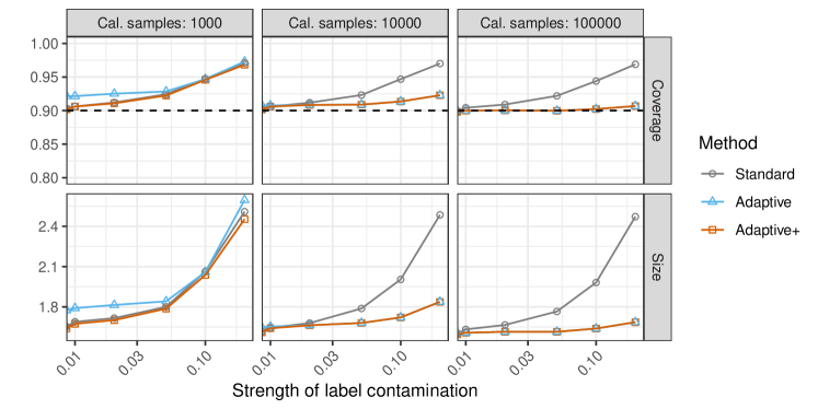
Figure A11: Performances of different conformal prediction methods with marginal coverage on simulated data with varying numbers of calibration samples, as a function of the label contamination strength. The dashed horizontal line indicates the 90% nominal marginal coverage level. Other details are as in Figure A2.

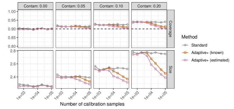
Figure A13: Performances of different conformal methods on simulated data with label contamination. The label contamination process has a random heterogeneous structure that tends to over-represent more common labels. The Adaptive+ method is applied with and without perfect knowledge of the label frequencies. Note that in this case there is some difference in performance because we approximate $\rho$ with $\tilde{\rho}$ even though in truth $\tilde{\rho}\neq\rho$. The nominal marginal coverage level is 90%. Other details are as in Figure A9.

A4.1.7 Prediction sets with calibration-conditional coverage

A4.2 Simulations under bounded label contamination

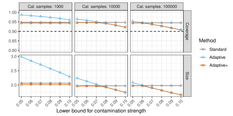
Figure A17: Performances of different conformal methods on simulated data with random label contamination, as a function of the known lower confidence bound for the contamination strength parameter $\epsilon=0.1$. The results are stratified based on the numbers of calibration samples. Other details are as in Figure 3.

A4.3 Simulations with estimated contamination strength

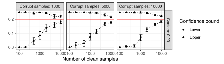
Figure A20: Bootstrap confidence intervals, for the label contamination strength parameter $\epsilon$, utilized by the Adaptive+ (CI) method in Figure A19.

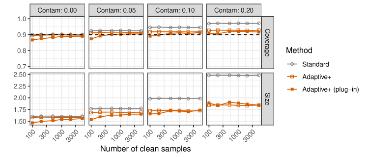
Figure A22: Performances of different conformal methods on simulated data with random label contamination, as a function of the number of clean samples used to fit the contamination model. The number of possible classes is $K=4$. Other details are as in Figure A21.

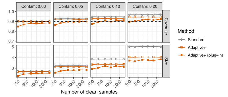
Figure A23: Performances of different conformal methods on simulated data with random label contamination, as a function of the number of clean samples used to fit the contamination model. The number of possible classes is $K=8$. Other details are as in Figure A21.

A4.4 Robustness to model mis-specification

A4.5 Demonstrations with CIFAR-10 image data

Appendix A5 Additional details on numerical experiments

A5.1 Experiments with heteroscedastic decision-tree model

We set $d=50$ and generate each sample of features $X\in\mathbb{R}^{d}$ independently as follows: $X_{1}=+1$ w.p. $3/4$, and $X_{1}=-1$ w.p. $1/4$; $X_{2}=+1$ w.p. $3/4$, and $X_{2}=-2$ w.p. $1/4$; $X_{3}=+1$ w.p. $1/4$, and $X_{3}=-2$ w.p. $1/2$; $X_{4}$ is uniformly distributed on $\{1,\ldots,4\}$; and $X_{j}\overset{i.i.d.}{\sim}\mathcal{N}(0,1)$ for all $j\in\{5,\ldots,d\}$. The labels $Y$ belong to one of $K=4$ possible classes, and their conditional distribution given $X=x$ is given by the decision tree shown in Figure A26, which only depends on the first four features.

Figure A26: A toy heteroscedastic decision-tree model for $P_{Y\mid X}$ used to generate syntheticin some numerical experiments.

References

• [1] Vladimir Vovk, Alex Gammerman and Glenn Shafer “Algorithmic learning in a random world” Springer, 2005
• [2] Nagarajan Natarajan, Inderjit S Dhillon, Pradeep K Ravikumar and Ambuj Tewari “Learning with noisy labels” In Advances in Neural Information Processing Systems 26, 2013
• [3] Sainbayar Sukhbaatar, Joan Bruna, Manohar Paluri, Lubomir Bourdev and Rob Fergus “Training convolutional networks with noisy labels” In preprint at arXiv:1406.2080, 2014
• [4] Yilun Xu, Peng Cao, Yuqing Kong and Yizhou Wang “L_dmi: A novel information-theoretic loss function for training deep nets robust to label noise” In Advances in Neural Information Processing Systems 32, 2019
• [5] Davood Karimi, Haoran Dou, Simon K Warfield and Ali Gholipour “Deep learning with noisy labels: Exploring techniques and remedies in medical image analysis” In Medical image analysis 65 Elsevier, 2020, pp. 101759
• [6] Michael A Hedderich, Lukas Lange, Heike Adel, Jannik Strötgen and Dietrich Klakow “A survey on recent approaches for natural language processing in low-resource scenarios” In preprint at arXiv:2010.12309, 2020
• [7] Curtis G Northcutt, Anish Athalye and Jonas Mueller “Pervasive label errors in test sets destabilize machine learning benchmarks” In preprint at arXiv:2103.14749, 2021
• [8] Görkem Algan and Ilkay Ulusoy “Image classification with deep learning in the presence of noisy labels: A survey” In Knowledge-Based Systems 215 Elsevier, 2021, pp. 106771
• [9] Hwanjun Song, Minseok Kim, Dongmin Park, Yooju Shin and Jae-Gil Lee “Learning from noisy labels with deep neural networks: A survey” In IEEE Transactions on Neural Networks and Learning Systems IEEE, 2022
• [10] Alexander Sorokin and David Forsyth “Utility data annotation with Amazon mechanical turk” In 2008 IEEE computer society conference on computer vision and pattern recognition workshops, 2008, pp. 1–8 IEEE
• [11] Cyrus Rashtchian, Peter Young, Micah Hodosh and Julia Hockenmaier “Collecting image annotations using Amazon’s mechanical turk” In Proceedings of the NAACL HLT 2010 workshop on creating speech and language data with Amazon’s Mechanical Turk, 2010, pp. 139–147
• [12] Panagiotis G Ipeirotis, Foster Provost and Jing Wang “Quality management on Amazon mechanical turk” In Proceedings of the ACM SIGKDD workshop on human computation, 2010, pp. 64–67
• [13] Rion Snow, Brendan O’connor, Dan Jurafsky and Andrew Y Ng “Cheap and fast–but is it good? evaluating non-expert annotations for natural language tasks” In Proceedings of the 2008 conference on empirical methods in natural language processing, 2008, pp. 254–263
• [14] Ryan Kennedy, Scott Clifford, Tyler Burleigh, Philip D Waggoner, Ryan Jewell and Nicholas JG Winter “The shape of and solutions to the MTurk quality crisis” In Political Science Research and Methods 8.4 Cambridge University Press, 2020, pp. 614–629
• [15] Herman Aguinis, Isabel Villamor and Ravi S Ramani “MTurk research: Review and recommendations” In Journal of Management 47.4 SAGE Publications Sage CA: Los Angeles, CA, 2021, pp. 823–837
• [16] Maxime Cauchois, Suyash Gupta, Alnur Ali and John Duchi “Predictive inference with weak supervision” In preprint at arXiv:2201.08315, 2022
• [17] Bat-Sheva Einbinder, Stephen Bates, Anastasios N Angelopoulos, Asaf Gendler and Yaniv Romano “Conformal Prediction is Robust to Label Noise” In preprint at arXiv:2209.14295, 2022
• [18] Vladimir Vovk, David Lindsay, Ilia Nouretdinov and Alex Gammerman “Mondrian Confidence Machine” On-line Compression Modelling project, On-line Compression Modelling project, 2003
• [19] Clayton Scott, Gilles Blanchard and Gregory Handy “Classification with asymmetric label noise: Consistency and maximal denoising” In Conference on learning theory, 2013, pp. 489–511 PMLR
• [20] Aritra Ghosh, Himanshu Kumar and P Shanti Sastry “Robust loss functions under label noise for deep neural networks” In Proceedings of the AAAI conference on artificial intelligence 31.1, 2017
• [21] Vladimir Vovk “Conditional Validity of Inductive Conformal Predictors” In Proceedings of the Asian Conference on Machine Learning 25, 2012, pp. 475–490
• [22] Yaniv Romano, Rina Foygel Barber, Chiara Sabatti and Emmanuel Candès “With Malice Toward None: Assessing Uncertainty via Equalized Coverage” In Harvard Data Science Review, 2020
• [23] Joshua C Peterson, Ruairidh M Battleday, Thomas L Griffiths and Olga Russakovsky “Human uncertainty makes classification more robust” In Proceedings of the IEEE/CVF International Conference on Computer Vision, 2019, pp. 9617–9626
• [24] Jing Lei, James Robins and Larry Wasserman “Distribution-Free Prediction Sets” In Journal of the American Statistical Association 108.501 Taylor & Francis, 2013, pp. 278–287 DOI: 10.1080/01621459.2012.751873.
• [25] Jing Lei and Larry Wasserman “Distribution-free prediction bands for non-parametric regression” In Journal of the Royal Statistical Society: Series B (Statistical Methodology) 76.1 Wiley Online Library, 2014, pp. 71–96
• [26] Jing Lei, Max G’Sell, Alessandro Rinaldo, Ryan J. Tibshirani and Larry Wasserman “Distribution-free predictive inference for regression” In Journal of the American Statistical Association 113.523 Taylor & Francis, 2018, pp. 1094–1111
• [27] James Smith, Ilia Nouretdinov, Rachel Craddock, Charles Offer and Alexander Gammerman “Conformal anomaly detection of trajectories with a multi-class hierarchy” In International symposium on statistical learning and data sciences, 2015, pp. 281–290 Springer
• [28] Leying Guan and Robert Tibshirani “Prediction and outlier detection in classification problems” In Journal of the Royal Statistical Society: Series B (Statistical Methodology) 84.2, 2022, pp. 524–546
• [29] Ziyi Liang, Matteo Sesia and Wenguang Sun “Integrative conformal p-values for powerful out-of-distribution testing with labeled outliers” In preprint at arXiv:2208.11111, 2022
• [30] Stephen Bates, Emmanuel Candès, Lihua Lei, Yaniv Romano and Matteo Sesia “Testing for outliers with conformal p-values” In Annals of Statistics 51.1 Institute of Mathematical Statistics, 2023, pp. 149–178
• [31] Meshi Bashari, Amir Epstein, Yaniv Romano and Matteo Sesia “Derandomized novelty detection with FDR control via conformal e-values” In preprint at arXiv:2302.07294, 2023
• [32] Yaniv Romano, Evan Patterson and Emmanuel J Candès “Conformalized quantile regression” In Advances in Neural Information Processing Systems, 2019, pp. 3538–3548
• [33] Matteo Sesia and Emmanuel J Candès “A comparison of some conformal quantile regression methods” In Stat 9.1 Wiley Online Library, 2020
• [34] Matteo Sesia and Yaniv Romano “Conformal Prediction using Conditional Histograms” In Advances in Neural Information Processing Systems 34, 2021
• [35] Yotam Hechtlinger, Barnabás Póczos and Larry Wasserman “Cautious Deep Learning” In preprint at arXiv:1805.09460, 2018
• [36] Mauricio Sadinle, Jing Lei and Larry Wasserman “Least ambiguous set-valued classifiers with bounded error levels” In Journal of the American Statistical Association 114.525 Taylor & Francis, 2019, pp. 223–234
• [37] Maxime Cauchois, Suyash Gupta and John C Duchi “Knowing what You Know: valid and validated confidence sets in multiclass and multilabel prediction.” In J. Mach. Learn. Res. 22, 2021, pp. 81–1
• [38] Yaniv Romano, Matteo Sesia and Emmanuel J. Candès “Classification with Valid and Adaptive Coverage” In Advances in Neural Information Processing Systems 33, 2020
• [39] Bat-Sheva Einbinder, Yaniv Romano, Matteo Sesia and Yanfei Zhou “Training Uncertainty-Aware Classifiers with Conformalized Deep Learning” In Adv. Neural Inf. Process. Syst. 35, 2022
• [40] Rina Foygel Barber, Emmanuel J Candès, Aaditya Ramdas and Ryan J Tibshirani “Conformal prediction beyond exchangeability” In preprint at arXiv:2202.13415, 2022
• [41] Ryan J Tibshirani, Rina Foygel Barber, Emmanuel Candes and Aaditya Ramdas “Conformal prediction under covariate shift” In Advances in Neural Information Processing Systems 32, 2019
• [42] Matteo Sesia and Stefano Favaro “Conformal frequency estimation with sketched data” In Advances in Neural Information Processing Systems 35, 2022, pp. 6589–6602
• [43] Isaac Gibbs and Emmanuel Candes “Adaptive conformal inference under distribution shift” In Advances in Neural Information Processing Systems 34, 2021, pp. 1660–1672
• [44] Isaac Gibbs and Emmanuel Candès “Conformal inference for online prediction with arbitrary distribution shifts” In preprint at arXiv:2208.08401, 2022
• [45] Cristina P Sison and Joseph Glaz “Simultaneous confidence intervals and sample size determination for multinomial proportions” In Journal of the American Statistical Association 90.429 Taylor & Francis, 1995, pp. 366–369
• [46] F. Pedregosa, G. Varoquaux, A. Gramfort, V. Michel, B. Thirion, O. Grisel, M. Blondel, P. Prettenhofer, R. Weiss, V. Dubourg, J. Vanderplas, A. Passos, D. Cournapeau, M. Brucher, M. Perrot and E. Duchesnay “Scikit-learn: Machine Learning in Python” In Journal of Machine Learning Research 12, 2011, pp. 2825–2830
• [47] I Guyon “Design of experiments for the NIPS 2003 variable selection benchmark 2003 [Available from: http://clopinet. com/isabelle/Projects” In NIPS2003
• [48] Alex Krizhevsky, Vinod Nair and Geoffrey Hinton “The CIFAR-10 dataset (2014)” In Online: http://www. cs. toronto. edu/kriz/cifar. html 55, 2020
• [49] Adam Paszke, Sam Gross, Francisco Massa, Adam Lerer, James Bradbury, Gregory Chanan, Trevor Killeen, Zeming Lin, Natalia Gimelshein and Luca Antiga “Pytorch: An imperative style, high-performance deep learning library” In Advances in Neural Information Processing Systems 32, 2019
• [50] Lihua Lei and Emmanuel J Candès “Conformal inference of counterfactuals and individual treatment effects” In Journal of the Royal Statistical Society Series B 83.5 Royal Statistical Society, 2021, pp. 911–938
• [51] Mingzhang Yin, Claudia Shi, Yixin Wang and David M Blei “Conformal sensitivity analysis for individual treatment effects” In Journal of the American Statistical Association Taylor & Francis, 2022, pp. 1–14
• [52] Emmanuel Candès, Lihua Lei and Zhimei Ren “Conformalized survival analysis” In Journal of the Royal Statistical Society Series B 85.1 Oxford University Press US, 2023, pp. 24–45
• [53] Matteo Sesia, Stefano Favaro and Edgar Dobriban “Conformal frequency estimation using discrete sketched data with coverage for distinct queries” In preprint at arXiv:2211.04612, 2022
• [54] Yu Gui, Rina Foygel Barber and Cong Ma “Conformalized matrix completion” In preprint at arXiv:2305.10637, 2023
• [55] Rina Foygel Barber, Emmanuel J Candès, Aaditya Ramdas and Ryan J Tibshirani “Predictive inference with the jackknife+” In Annals of Statistics 49.1 Institute of Mathematical Statistics, 2021, pp. 486–507