Detecting Violations of Differential Privacy for Quantum Algorithms

Abstract.

Quantum algorithms for solving a wide range of practical problems have been proposed in the last ten years, such as data search and analysis, product recommendation, and credit scoring. The concern about privacy and other ethical issues in quantum computing naturally rises up. In this paper, we define a formal framework for detecting violations of differential privacy for quantum algorithms. A detection algorithm is developed to verify whether a (noisy) quantum algorithm is differentially private and automatically generates bugging information when the violation of differential privacy is reported. The information consists of a pair of quantum states that violate the privacy, to illustrate the cause of the violation. Our algorithm is equipped with Tensor Networks, a highly efficient data structure, and executed both on TensorFlow Quantum and TorchQuantum which are the quantum extensions of famous machine learning platforms — TensorFlow and PyTorch, respectively. The effectiveness and efficiency of our algorithm are confirmed by the experimental results of almost all types of quantum algorithms already implemented on realistic quantum computers, including quantum supremacy algorithms (beyond the capability of classical algorithms), quantum machine learning models, quantum approximate optimization algorithms, and variational quantum eigensolvers with up to 21 quantum bits.

1. Introduction

Quantum Algorithms and Quantum Machine Learning Models: A quantum algorithm is an algorithm that runs on a realistic model of quantum computation. The most commonly used quantum computational model is the quantum circuit model. A series of quantum algorithms have been proposed to speed up the classical counterparts to solve fundamental problems, such as Grover’s algorithm (grover1996fast, ) for searching an unstructured database, Shor’s algorithm (shor1994algorithms, ) for finding the prime factors of an integer and HHL (Aram Harrow, Avinatan Hassidim, and Seth Lloyd) algorithm (harrow2009quantum, ) for solving systems of linear equations. In recent years, motivated by the huge success of classical machine learning models in practical applications, quantum machine learning models (also known as well-trained quantum machine learning algorithms) are proposed to accelerate solving the same classical tasks. Specifically, like the classical models, a bulk of corresponding quantum learning models have been defined and trained on existing quantum hardware or simulators of quantum computation on classical supercomputers. Examples include quantum support vector machines (Rebentrost2014, ), quantum convolution neural networks (cong2019quantum, ), quantum recurrent neural networks (bausch2020recurrent, ), quantum generative adversarial networks (dallaire2018quantum, ) and quantum reinforcement learning networks (dong2008quantum, ). Subsequently, these models have been tested to solve a wide range of real-world problems, such as fraud detection (in transaction monitoring) (liu2018quantum, ; di2021quantum, ), credit assessments (risk scoring for customers) (unknown, ; milne2017optimal, ) and handwritten digit recognition (broughton2020tensorflow, ). On the other hand, a series of quantum machine learning algorithms without the classical counterparts have also been designed to solve specific problems. For example, quantum approximate optimization algorithm (QAOA) is a toy model of quantum annealing and is used to solve problems in graph theory (farhi2014quantum, ), variational quantum eigensolver (VQE) applies classical optimization to minimize the energy expectation of an ansatz state to find the ground state energy of a molecule (peruzzo2014variational, ). Furthermore, based on the famous classical machine learning training platforms — TensorFlow and Pytorch, two quantum training platforms have been established: TensorFlow Quantum (broughton2020tensorflow, ) and TorchQuantum (wang2022quantumnas, ), respectively.

The rapid development of quantum hardware enables those more and more experimental implementations of the algorithms mentioned above on concrete problems have been achieved (google2020hartree, ; harrigan2021quantum, ). Notably, quantum supremacy (or advantage beyond classical computation) was proved by Google’s quantum computer Sycamore with 53 noisy superconducting qubits (quantum bits) that can do a sampling task in 200 seconds, while the same task would cost (arguably) 10,000 years on the largest classical computer (arute2019quantum, ). A type of Boson sampling was performed on USTC’s quantum computer Jiuzhang with 76 noisy photonic qubits in 20 seconds that would take 600 million years for a classical computer (zhong2020quantum, ). These experiments demonstrate the power of quantum computers with tens to hundreds of qubits in the current Noisy Intermediate-Scale Quantum (NISQ) era where quantum noises cannot be avoided. Meanwhile, more and more quantum cloud computing platforms (e.g. IBM’s Qiskit Runtime and Microsoft’s Azure Quantum) are available for public use to implement quantum algorithms on realistic quantum chips.

Differential Privacy: From Classical to Quantum: Differential privacy has become a de facto standard evaluating an algorithm for protecting the privacy of individuals. It ensures that any individual’s information has very little influence on the output of the algorithm. Based on this intuition, the algorithmic foundation of differential privacy in classical (machine learning) algorithms has been established (dwork2014algorithmic, ; ji2014differential, ). However, developing algorithms with differentially private guarantees is very subtle and error-prone. Indeed, a large number of published algorithms violate differential privacy. This situation boosts the requirement of a formal framework for verifying the differential privacy of classical algorithms. Various verification techniques have been extended into this context  (barthe2013verified, ; barthe2016advanced, ; barthe2014proving, ; barthe2016proving, ; barthe2012probabilistic, ; barthe2013beyond, ). Furthermore, a counterexample generator for the failure in the verification can be provided for the debugging purpose (ding2018detecting, ).

With more and more applications, the privacy issue of quantum algorithms also rises. Indeed, from the viewpoint of applications, this issue is even more serious than its classical counterpart since it is usually hard for the end users to understand quantum algorithms. Inspired by its great success in applications, the notion of differential privacy has recently been extended to quantum computation, and some fundamental algorithmic results for computing privacy parameters have been obtained (zhou2017differential, ; aaronson2019gentle, ; hirche2022quantum, ) in terms of different definitions of the similarity between quantum states. However, the verification and violation detecting problem of differential privacy of quantum algorithms have not been touched in the previous works.

Contributions of This Paper: In this work, we define a formal framework for the verification of differential privacy for quantum algorithms in a principled way. Specifically, our main contributions are as follows:

1. Algorithm: An algorithm for detecting violations of differential privacy for quantum algorithms is developed. More specifically, this algorithm can not only efficiently check whether or not a (noisy) quantum algorithm is differentially private, but also automatically generate a pair of quantum states when the violation of differential privacy is reported. These two states that break the promising differential privacy provide us with debugging information.

2. Case Studies: Our detection algorithm is implemented both on TensorFlow Quantum (broughton2020tensorflow, ) and TorchQuantum (wang2022quantumnas, ) which are based on famous machine learning platforms — TensorFlow and PyTorch, respectively. The effectiveness and efficiency of our algorithm are confirmed by the experimental results of almost all types of quantum algorithms already implemented on realistic quantum computers, including quantum supremacy algorithms (beyond the capability of classical algorithms), quantum machine learning models, quantum approximate optimization algorithms, and variational quantum eigensolver algorithms with up to 21 qubits.

3. Byproducts: We show that quantum noises can be used to protect the privacy of quantum algorithms as in the case of classical algorithms, and establish a composition theorem of quantum differential privacy for handling larger quantum algorithms in a modular way.

1.1. Related Works and Challenges

Detecting Violations for Classical Algorithms: Detecting the violations of differential privacy for classical (randomized) algorithms has been studied in (ding2018detecting, ). Their approach is to analyze the (distribution of) outputs of classical algorithms in a statistical way. Specifically, it runs a candidate algorithm many times and uses statistical tests to detect violations of differential privacy. However, such a method has some limitations: if an algorithm satisfies differential privacy except with an extremely small probability then it may not detect the violations. To avoid this situation appearing in the quantum world, we introduce a series of linear algebra operations to analyze the output states of quantum algorithms. In particular, we characterize the verification of differential privacy as inequalities and solve them by computing eigenvalues and eigenvectors of some matrices, which are indexed by a quantum measurement outcome and represent the converse (dual) implementation of quantum algorithms. As a result, our developed verification algorithm is exact (sound and complete).

Differential Privacy for Quantum Circuits: Quantum differential privacy was first defined in (zhou2017differential, )-(hirche2022quantum, ) for (noisy) quantum circuits. However, the verification and violation detection problems for quantum differential privacy were not addressed there.

In this paper, we adapt the quantum differential privacy for quantum algorithms rather than quantum circuits, motivated mainly by our target applications. Roughly speaking, a quantum algorithm can be thought of as a quantum circuit together with a quantum measurement at the end to extract the computational outcome (classical information). Accordingly, the privacy for a circuit must be examined for all possible measurements, but the privacy for an algorithm should be defined for a fixed measurement. This subtle difference leads to different verification problems and solutions. In the case of algorithms, the verification problem can be solved by transferring the impact of algorithmic steps on input quantum states to the given quantum measurement. But it seems that the same idea cannot be applied to the case of circuits because the final measurement is unknown beforehand. On the other hand, the counterexample generator of differential privacy constructed in this paper can be used to detect differential privacy violations in quantum circuits by appending certain measurements to them.

2. Preliminaries

In this section, for the convenience of the reader, we introduce basic ideas of quantum algorithms in a mathematical way.

Roughly speaking, a quantum algorithm consists of a quantum circuit and a quantum measurement. The former is for implementing algorithmic instructions; the latter is to extract the classical information from the final state at the end of the circuit. The computational components in the quantum algorithm can be mathematically described by two types of matrices: (i) unitary matrices for quantum gates and circuits; and (ii) positive semi-definite matrices for density operators (quantum states) and (Positive Operator-Valued Measure) quantum measurements. Thus we start with a brief introduction of these two kinds of matrices in the context of quantum computation.

2.1. Unitary and Positive Semi-definite Matrices

Before defining unitary and positive semi-definite matrices, we need to specify the state space we are interested in. Mathematically, a quantum algorithm works on a $2^{n}$-dimensional Hilbert (linear) space $\mathcal{H}$, where $n$ is the number of quantum bits (qubits) (defined in the next section) involved in the algorithm. Thus, in this paper, all linear algebra operations are based on $\mathcal{H}$. We choose to use standard quantum mechanical notation instead of that from linear algebra. This style of notation is known as the Dirac notation, and widely used in the field of quantum computation. For more details, we refer to textbook (nielsen2010quantum, ).

First of all, vectors in $\mathcal{H}$ can be represented as the following Dirac notations:

1. $\ket{\psi}$ stands for a $2^{n}$-dimensional complex unit (normalized) column vector in $\mathcal{H}$ labelled with $\psi$;

2. $\bra{\psi}:=\ket{\psi}^{\dagger}$ is the Hermitian adjoint (complex conjugate and transpose) of $\ket{\psi}$;

3. $\braket{\psi_{1}}{\psi_{2}}:=(\ket{\psi_{1}},\ket{\psi_{2}})$ is the inner product of $\ket{\psi_{1}}$ and $\ket{\psi_{2}}$;

4. $|\psi_{1}\rangle\langle\psi_{2}|$ is the outer product;

5. $\ket{\psi_{1},\psi_{2}}:=\ket{\psi_{1}}\ket{\psi_{2}}$ is a shorthand of the product state $\ket{\psi_{1}}\otimes\ket{\psi_{2}}$.

Unitary Matrices: In the ($2^{n}$-dimensional) Hilbert space $\mathcal{H}$, a unitary matrix $U$ is a $2^{n}\times 2^{n}$ matrix with $U^{\dagger}U=UU^{\dagger}=I_{n}$, where $U^{\dagger}=(U^{*})^{\top}$ is the (entry-wise) conjugate transpose of $U$ and $I_{n}$ is the identity matrix on $\mathcal{H}$.

Positive Semi-Definite Matrices: A $2^{n}\times 2^{n}$ matrix $M$ is called positive semi-definite if for any $\ket{\psi}\in\mathcal{H}$, $\bra{\psi}M\ket{\psi}\geq 0$. Subsequently, all eigenvalues of $M$ are non-negative. That is, for any unit eigenvector $\ket{\psi}$ of $M$ ( i.e., $M\ket{\psi}=\lambda\ket{\psi}$), we have $\lambda\geq 0$.

Some examples of these two matrices with physical meanings will be provided in the next section for a better understanding.

2.2. Quantum Algorithms

Now we turn to review the setup of quantum algorithms in their most basic form. A quantum algorithm is a set of instructions solving a problem (e.g., Shor’s algorithm for finding the prime factors of an integer) that can be performed on a quantum computer. Physically, the algorithm is implemented by a quantum circuit that can be executed on quantum hardware. The computational flow of the quantum algorithm is drawn in the following.

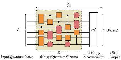
Figure 1. The Computational Model of Quantum Algorithms.

With the notions introduced in the above subsection, we can explain the above procedures from the left side to the right one.

Input Quantum States: An input can be a pure quantum state, which is mathematically modeled as a complex unit column vector $\ket{\psi}$ in a $2^{n}$-dimensional Hilbert (linear) space $\mathcal{H}$, where $n$ denotes the number of qubits in $\ket{\psi}$. For example, a state of a qubit is a vector in a $2$-dimensional Hilbert space, written in the Dirac notation as

$$\ket{q}=\left(\begin{array}[]{cc}a\\ b\end{array}\right)=a\ket{0}+b\ket{1}\ {\rm with}\ \ket{0}=\left(\begin{array}[]{cc}1\\ 0\end{array}\right)\text{ and }\ket{1}=\left(\begin{array}[]{cc}0\\ 1\end{array}\right),$$

where complex numbers $a$ and $b$ satisfy the normalization condition $|a|^{2}+|b|^{2}=1$. Here, the orthonormal basis $\ket{0}$, $\ket{1}$ of the Hilbert space corresponds to the digital value $0$, $1$ of a bit in classical computers, respectively.

On a NISQ hardware, noises are unavoidable, and a pure state $\ket{\psi}$ on $\mathcal{H}$ may collapse into a mixed state, represented as an ensemble $\{(p_{k},\ket{\psi_{k}})\}_{k}$, meaning that it is in $\ket{\psi_{k}}$ with probability $p_{k}$. Mathematically, the ensemble can be described by a $2^{n}\times 2^{n}$ positive semi-definite matrix:

$$\rho=\sum_{k}p_{k}|\psi_{k}\rangle\langle\psi_{k}|$$

with unit trace in the $2^{n}$-dimensional Hilbert (linear) space $\mathcal{H}$, i.e., ${\rm tr}(\rho)=1$, where trace ${\rm tr}(\rho)$ of $\rho$ is defined as the summation of diagonal elements of $\rho$. We use $\mathcal{D(H)}$ to denote the set of all (mixed) quantum states in $\mathcal{H}$.

(Noisy) Quantum Circuits: The computational part (without the final measurement) of a quantum algorithm can be described by a quantum circuit. A quantum circuit $U$ consists of a sequence (product) of quantum logic gates $U_{i}$, i.e., $U=U_{d}\cdots U_{1}$ ( See the orange boxes of the quantum circuit in Fig. 1). Here $d$ is the depth of the circuit $U$, and each $U_{i}$ is mathematically modeled by a unitary matrix. For an input $n$-qubit state $\rho$, the output of the circuit is a quantum state of the same size:

(1) $$\rho^{\prime}=U\rho U^{\dagger}.$$

Example 2.1.

A set of typical quantum logic gates used in this paper are listed in the following.

• 1-qubit (parameterized) logic gates ($2\times 2$ unitary matrices):

  $$\begin{aligned} X&=\begin{pmatrix}0&1\\ 1&0\end{pmatrix}&Y&=\begin{pmatrix}0&-i\\ i&0\end{pmatrix}&Z&=\begin{pmatrix}1&0\\ 0&-1\end{pmatrix}\\ H&=\frac{1}{\sqrt{2}}\begin{pmatrix}1&1\\ 1&-1\end{pmatrix}&S&=\begin{pmatrix}1&0\\ 0&i\end{pmatrix}&T&=\begin{pmatrix}1&0\\ 0&e^{i\pi/4}\end{pmatrix}.\end{aligned}$$

• 1-qubit rotation gates that are rotation operators along $x,y,z$-axis by angle $\theta$, respectively:

  $$\begin{aligned} R_{x}(\theta)&=e^{-i\theta X/2}=\cos\frac{\theta}{2}I-i\sin\frac{\theta}{2}X=\begin{pmatrix}\cos\frac{\theta}{2}&-i\sin\frac{\theta}{2}\\ -i\sin\frac{\theta}{2}&\cos\frac{\theta}{2}\end{pmatrix}\\ R_{y}(\theta)&=e^{-i\theta Y/2}=\cos\frac{\theta}{2}I-i\sin\frac{\theta}{2}Y=\begin{pmatrix}\cos\frac{\theta}{2}&-\sin\frac{\theta}{2}\\ \sin\frac{\theta}{2}&\cos\frac{\theta}{2}\end{pmatrix}\\ R_{z}(\theta)&=e^{-i\theta Z/2}=\cos\frac{\theta}{2}I-i\sin\frac{\theta}{2}Z=\begin{pmatrix}e^{-i\theta/2}&0\\ 0&e^{i\theta/2}\end{pmatrix}.\end{aligned}$$

  Rotation gates $R_{x}(\theta),R_{y}(\theta),R_{z}(\theta)$ are widely used to encode classical data into quantum states and also construct quantum machine learning models (parameterized quantum circuits). These will be detailed in the later discussion.

• 2-qubit Controlled-U gates ($4\times 4$ unitary matrices): For any 1-qubit logic gate $U$, we can get a 2-qubit logic gate — controlled-$U$ (CU) gate, applying $U$ on the second qubit (the target qubit) if and only if the first qubit (the control qubit) is $\ket{1}$. See the following instances:

  1. CNOT: CX gate is also known as controlled NOT (CNOT) gate and has a special circuit representation:

     $$\text{CX}=\quantikz[rowsep=2.2mm,columnsep=2.3mm,]&\ctrl{1}\qw\\ \targ{}\qw=\begin{pmatrix}1&0&0&0\\ 0&1&0&0\\ 0&0&0&1\\ 0&0&1&0\end{pmatrix}.$$

  2. CZ gate:

     $$\text{CZ}=\quantikz[rowsep=2.2mm,columnsep=2.3mm,]&\ctrl{1}\qw\\ \control\qw\qw=\begin{pmatrix}1&0&0&0\\ 0&1&0&0\\ 0&0&1&0\\ 0&0&0&-1\end{pmatrix}$$

  3. Controlled parameterized gates: For example, the controlled Pauli X rotation gate with rotation angle $\theta$ is:

     $$\quantikz[rowsep=2.2mm,columnsep=2.3mm,]&\ctrl{1}\qw\\ \gate{R_{x}(\theta)}\qw=\begin{pmatrix}1&0&0&0\\ 0&1&0&0\\ 0&0&\cos\frac{\theta}{2}&-i\sin\frac{\theta}{2}\\ 0&0&-i\sin\frac{\theta}{2}&\cos\frac{\theta}{2}\end{pmatrix}$$

(a) A simple quantum neural network to perform MNIST image classification task in TorchQuantum’s tutorial.

[row sep=2.2mm, column sep=2.3mm,] & H T[4,steps=6,style=draw=white,dashed, rounded corners, inner xsep=0pt, background] 1 T 2
H T 2 T
H 1T SX
H T T

(b) A quantum supremacy algorithm with a $2\times 2$ qubits layout with four layers.

Figure 2. Examples of Quantum Machine Learning and Supremacy Algorithms

In quantum circuits, each quantum gate $U_{i}$ only non-trivially operates on one or two qubits. For example, if $U_{i}$ represents a Hadamard gate on the first qubit, then $U_{i}=H\otimes I_{n-1}$, where $I_{n-1}$ is a $2^{n-1}\times 2^{n-1}$ identity matrix applied on the rest $n-1$ qubits. See the gates in Figure 2.

In the current NISQ era, a (noiseless) quantum circuit $U$ can only have a noisy implementation modeled by a linear mapping $\mathcal{E}$ from $\mathcal{D(H)}$ to $\mathcal{D(H)}$ satisfying the following two conditions:

• $\mathcal{E}$ is trace-preserving: ${\rm tr}(\mathcal{E}(\rho))={\rm tr}(\rho)$ for all $\rho\in\mathcal{D(H)}$;

• $\mathcal{E}$ is completely positive: for any Hilbert space $\mathcal{H}^{\prime}$, the trivially extended operator $\operatorname{id}_{\mathcal{H}^{\prime}}\otimes\mathcal{E}$ maps density operators to density operators on $\mathcal{H}^{\prime}\otimes\mathcal{H}$, where $\operatorname{id}_{\mathcal{H}^{\prime}}$ is the identity map on $\mathcal{H}^{\prime}$: $\operatorname{id}_{\mathcal{H}^{\prime}}(\rho)=\rho$ for all $\rho\in\mathcal{D(H^{\prime})}$.

Such a mapping $\mathcal{E}$ is called a super-operator in the field of quantum computing and admits a Kraus matrix form (nielsen2010quantum, ): there exists a finite set $\{E_{k}\}_{k\in\mathcal{K}}$ of matrices on $\mathcal{H}$ such that

$$\mathcal{E}(\rho)=\sum_{k\in\mathcal{K}}E_{k}\rho E_{k}^{\dagger}\quad\textrm{ with }\sum_{k\in\mathcal{K}}E_{k}^{\dagger}E_{k}=I_{n},$$

where $\{E_{k}\}_{k\in\mathcal{K}}$ is called Kraus matrices of $\mathcal{E}$. In this case, $\mathcal{E}$ is often represented as $\mathcal{E}=\{E_{k}\}_{k\in\mathcal{K}}$. Thus, for an input state $\rho$ fed into the noisy quantum circuit $\mathcal{E}$, the output state is:

(2) $$\rho^{\prime}=\mathcal{E}(\rho).$$

If $\mathcal{E}$ degenerates to a unitary matrix $U$, i.e., $\mathcal{E}=\{U\}$, then the above equation (evolution) is reduced to the noiseless case in Eq. (1). Briefly, we write such $\mathcal{E}=\{U\}$ as $\mathcal{U}=\{U\}$ representing noiseless quantum circuit $U$.

Similarly to a noiseless quantum circuit $U$, a noisy quantum circuit $\mathcal{E}$ also consists of a sequence (mapping composition) of quantum logic (noisy) gates $\{\mathcal{E}_{i}\}$, i.e., $\mathcal{E}=\mathcal{E}_{d}\circ\cdots\circ\mathcal{E}_{1}$, where each $\mathcal{E}_{i}$ is either a noiseless quantum logic gate or a noisy one (e.g., the red dashed boxes of the noisy quantum circuit in Fig. 1). See the following examples of quantum noisy logic gates in a mathematical way.

Example 2.2.

Let us consider the following noise forming of a 1-qubit gate $U$:

$$\mathcal{E}_{U,p}(\rho)=(1-p)\rho+pU\rho U^{\dagger},\quad\forall\rho\in\mathcal{D(H)}$$

where $0\leq p\leq 1$ is a probability measuring the noisy level (effect) and $U$ is a unitary matrix. Then $\mathcal{E}_{U,p}$ consists of Kraus matrices $\{\sqrt{1-p}I,\sqrt{p}U\}$. Such $\mathcal{E}_{U,p}$ can be used to model several typical 1-qubit noises, depending on the choice of $U$: $U=X$ for bit flip, $U=Z$ for phase flip and $U=Y=iXZ$ for bit-phase flip (nielsen2010quantum, , Section 8.3). The depolarizing noise combines these three noises. It is represented by

$$\mathcal{E}_{D,p}=\{\sqrt{1-p}I,\sqrt{\frac{p}{3}}X,\sqrt{\frac{p}{3}}Y,\sqrt{\frac{p}{3}}Z\},$$

or equivalently

$$\mathcal{E}_{D,p}(\rho)=(1-p)\rho+\frac{p}{3}(X\rho X+Y\rho Y+Z\rho Z),\quad\forall\rho\in\mathcal{D(H)}.$$

Quantum Measurement: At the end of each quantum algorithm, a quantum measurement is set to extract the computational outcome (classical information). Such information is a probability distribution over the possible outcomes of the measurement. Mathematically, a quantum measurement is modeled by a set $\{M_{k}\}_{k\in\mathcal{O}}$ of positive semi-definite matrices on its state (Hilbert) space $\mathcal{H}$ with $\sum_{k}M_{k}=I$, where $\mathcal{O}$ is a finite set of the measurement outcomes. This observing process is probabilistic: if the output of the quantum circuit before the measurement is quantum state $\rho$, then a measurement outcome $k$ is obtained with probability

(3) $$p_{k}={\rm tr}(M_{k}\rho).$$

Such measurements are known as Positive Operator-Valued Measures and are widely used to describe the probabilities of outcomes without concerning the post-measurement quantum states (note that after the measurement, the state will be collapsed (changed), depending on the measurement outcome $k$, which is fundamentally different from the classical computation.)

By summarizing the above ideas, we obtain a general model of quantum algorithms as depicted in Fig. 1:

Definition 2.3.

A quantum algorithm $\mathcal{A}=(\mathcal{E},\{M_{k}\}_{k\in\mathcal{O}})$ is a randomized mapping $\mathcal{A}:\mathcal{D(H)}\rightarrow\mathcal{D(O)}$ defined by

$$\mathcal{A}(\rho)=\left\{{\rm tr}(M_{k}\mathcal{E}(\rho))\right\}_{k\in\mathcal{O}}\quad\forall\rho\in\mathcal{D(H)},$$

where:

1. $\mathcal{E}$ is a super-operator on Hilbert space $\mathcal{H}$ representing a noisy quantum circuit;

2. $\{M_{k}\}_{k\in\mathcal{O}}$ is a quantum measurement on $\mathcal{H}$ with $\mathcal{O}$ being the set of measurement outcomes (classical information);

3. $\mathcal{D(O)}$ stands for the set of probability distributions over $\mathcal{O}$.

In particular, if $\mathcal{E}$ represents a noiseless quantum circuit $U$ written as $\mathcal{U}=\{U\}$, then we call $\mathcal{A}=(\mathcal{U},\{M_{k}\}_{k\in\mathcal{O}})$ a noiseless quantum algorithm.

According to the above definition, a quantum algorithm $\mathcal{A}=(\mathcal{E},\{M_{k}\}_{k\in\mathcal{O}})$ is a randomized mapping, and thus we can estimate not only the distribution $\{{\rm tr}(M_{k}\mathcal{E}(\rho))\}_{k\in\mathcal{O}}$ but also the summation $\sum_{k\in\mathcal{S}}\{{\rm tr}(M_{k}\mathcal{E}(\rho))\}_{k\in\mathcal{O}}$ for any subset $\mathcal{S}\subseteq\mathcal{O}$ in a statistical way. This observation is essential in defining differential privacy for quantum algorithms in the next section.

Quantum Encoding: To make quantum algorithms useful for solving practical classical problems, the first step is to encode classical data into quantum states. There are multiple encoding methods, but amplitude encoding and angle encoding are two of the most widely used.

• Amplitude encoding represents a vector $\bar{v}$ as a quantum state $|\bar{v}\rangle$, using the amplitudes of the computational basis states $|i\rangle$:

  $$\bar{v}=(v_{1},v_{2},\ldots,v_{N})\rightarrow|\bar{v}\rangle=\sum_{i=1}^{N}\frac{v_{i}}{\|\bar{v}\|}|i\rangle$$

  where $\|\bar{v}\|$ normalizes the state. This encoding uses only $\log_{2}N$ qubits to represent an $N$-dimensional vector. However, preparing the state $|\bar{v}\rangle$ requires a deep, complex circuit beyond the current NISQ hardwares.

• Angle encoding encodes a vector $\bar{v}$ by rotating each qubit by an angle corresponding to one element of $\bar{v}$:

  $$\bar{v}=(v_{1},v_{2},\ldots,v_{n})\rightarrow\ket{\bar{v}}=\bigotimes_{j=1}^{n}R(v_{j})\ket{0}$$

  where $R(v_{j})$ rotates qubit $j$ by angle $v_{j}$ along some axis, i.e., $R$ can be one of $R_{x},R_{y},R_{z}$. This encoding uses $n$ qubits for an $n$-dimensional vector but only requires simple 1-qubit rotation gates. As an example, encoding $\bar{v}=(\pi,\pi,\pi)$ via $R_{y}$ rotations yields $\ket{\bar{v}}=\ket{1,1,1}=\ket{1}\otimes\ket{1}\otimes\ket{1}$. A key advantage of angle encoding is its parallelizability. Each qubit undergoes a rotation gate simultaneously, enabling encoding in constant time as shown in the following. This makes angle encoding well-suited for the current NISQ devices. Therefore, angle encoding is commonly used in the experimental implementation of quantum algorithms on existing quantum computers for solving classical computational tasks.

      

With the above encoding methods for pure state $\ket{\bar{v}}$, we can simply obtain a mixed state to carry the classical data $\bar{v}$:

$$\rho_{\bar{v}}=|\bar{v}\rangle\langle\bar{v}|.$$

In this paper, we consider the differential privacy of quantum algorithms on NISQ computers. As such, all of our experiments in the Evaluation section (Section 5) use angle encoding to encode classical data, including credit records, public adult income dataset, and transactions dataset.

3. Formalizing Differential Privacy

In this section, we introduce the differential privacy for quantum algorithms and clarify the relationship between it and the differential privacy for quantum circuits defined in (zhou2017differential, ). For the convenience of the reader, we put all proofs of theoretical results in the appendix.

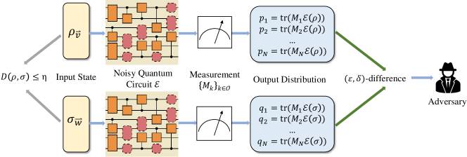
Figure 3. Quantum Differential Privacy

Let us start by defining the differential privacy for quantum algorithms:

Definition 3.1 (Differential Privacy for Quantum Algorithms).

Suppose we are given a quantum algorithm $\mathcal{A}=(\mathcal{E},\{M_{k}\}_{k\in\mathcal{O}})$ on a Hilbert space $\mathcal{H}$, a distance metric $D(\cdot,\cdot)$ on $\mathcal{D(H)}$, and three small enough threshold values $\varepsilon,\delta,\eta\geq 0$. Then $\mathcal{A}$ is said to be $(\varepsilon,\delta)$-differentially private within $\eta$ if for any quantum states $\rho,\sigma\in\mathcal{D(H)}$ with $D(\rho,\sigma)\leq\eta$, and for any subset $\mathcal{S}\subseteq\mathcal{O}$, we have

(4) $$\sum_{k\in\mathcal{S}}{\rm tr}(M_{k}\mathcal{E}(\rho))\leq\exp(\varepsilon)\sum_{k\in\mathcal{S}}{\rm tr}(M_{k}\mathcal{E}(\sigma))+\delta.$$

In particular, if $\delta=0$, we say that $\mathcal{A}$ is $\varepsilon$-differentially private within $\eta$.

The above definition is essentially a quantum generalization of differential privacy for randomized algorithms (dwork2014algorithmic, ). Thus, it shares the intuition of differential privacy discussed in (dwork2014algorithmic, ): an algorithm must behave similarly on similar input states (considered as neighbors in the state space). In the quantum case, we have:

1. $\eta$ defines the (noisy) neighboring relation between the two input states $\rho$ and $\sigma$, i.e., $D(\rho,\sigma)\leq\eta$;

2. $\varepsilon$ and $\delta$ through Eq.(4) guarantee the similarity between the outputs of $\sum_{k\in\mathcal{S}}{\rm tr}(M_{k}\mathcal{E}(\rho))$ and $\sum_{k\in\mathcal{S}}{\rm tr}(M_{k}\mathcal{E}(\sigma))$;

3. Since a quantum algorithm is a randomized function, it is reasonable to consider the probability $\sum_{k\in\mathcal{S}}{\rm tr}(M_{k}\mathcal{E}(\rho))$ that the output is within a subset $\mathcal{S}\subseteq\mathcal{O}$ rather than an exact value of ${\rm tr}(M_{k}\mathcal{E}(\rho))$. The arbitrariness of $\mathcal{S}\subseteq\mathcal{O}$ in Eq.(4) ensures the differential privacy in randomized functions as the same as in the classical case (dwork2014algorithmic, ).

Consequently, quantum differential privacy ensures that the indistinguishabilities of any neighboring quantum states are kept by quantum algorithms. Specifically, as shown in Fig. 3, an adversary is hard to determine whether the input state of the algorithm was indeed $\rho$ or a neighboring state $\sigma$ such that the information revealed in the $(\varepsilon,\delta)$-difference between $\rho$ and $\sigma$ in Eq. (4) cannot be easily inferred by observing the output measurement distribution of the algorithm. Furthermore, quantum encoding allows quantum states to encode classical data, so $\rho$ and $\sigma$ can be regarded as $\rho_{\bar{v}}$ and $\sigma_{\bar{w}}$ which encodes classical vectors $\bar{v}$ and $\bar{w}$. Thus the distance bound $\eta$ between $\rho_{\bar{v}}$ and $\sigma_{\bar{w}}$ can be used to represent the single element difference of classical data $\bar{v}$ and $\bar{w}$. Thus classical neighboring relation can be preserved by the quantum counterpart. Therefore, quantum differential privacy can be used as a proxy to ensure the original motivating privacy that the presence or absence of any individual data record will not significantly affect the outcome of an analysis. A concrete example is provided to detail this in the later of this section. Furthermore, this idea will be utilized in our case studies in Section 5 to demonstrate how quantum noise can enhance the privacy of encoded classical data.

It is easy to see that when considering noiseless trivial quantum circuits (i.e., $\mathcal{E}=\text{id}_{\mathcal{H}}$, the identity map on $\mathcal{H}$), the above setting degenerates to Aaronson and Rothblum’s framework (aaronson2019gentle, ) where an elegant connection between quantum differential privacy and gentle measurements was established. In this paper, we consider a more general class of measurements, and a connection between quantum measurements and the verification of quantum differential privacy under quantum noise is revealed.

By Definition 3.1, if a quantum algorithm $\mathcal{A}=(\mathcal{E},\{M_{k}\}_{k\in\mathcal{O}})$ is not $(\varepsilon,\delta)$-differentially private, then there exists at least one pair of quantum states $(\rho,\sigma)$ with the distance of them being within $\eta$, i.e., $D(\rho,\sigma)\leq\eta$, and a subset $\mathcal{S}\subseteq\mathcal{O}$ such that

(5) $$\sum_{k\in\mathcal{S}}{\rm tr}(M_{k}\mathcal{E}(\rho))>\exp(\varepsilon)\sum_{k\in\mathcal{S}}{\rm tr}(M_{k}\mathcal{E}(\sigma))+\delta.$$

Such a pair of quantum states $(\rho,\sigma)$ is called a $(\varepsilon,\delta)$-differentially private counterexample of $\mathcal{A}$ within $\eta$.

Figure 4. The relationship between the differential privacy (DP) for quantum circuits (QCs) and quantum algorithms (QAs)

As said before, the notion of differential privacy for (noisy) quantum circuits has been defined in the previous works (zhou2017differential, ; hirche2022quantum, ). Using Definition 3.1, it can be reformulated as the following:

Definition 3.2 (Differential Privacy for Quantum Circuits).

Suppose we are given a (noisy) quantum circuit $\mathcal{E}$ on a Hilbert space $\mathcal{H}$, a distance metric $D(\cdot,\cdot)$ on $\mathcal{D(H)}$, and three small enough threshold values $\varepsilon,\delta,\eta\geq 0$. Then $\mathcal{E}$ is said to be $(\varepsilon,\delta)$-differentially private within $\eta$ if for any quantum measurement $\{M_{k}\}_{k\in\mathcal{O}}$, the algorithm obtained from $\mathcal{E}$ by adding the measurement at the end, i.e. $(\mathcal{E},\{M_{k}\}_{k\in\mathcal{O}})$, is $(\varepsilon,\delta)$-differentially private within $\eta$.

The relationship between differential privacy for quantum algorithms and quantum circuits can be visualized as Fig 4. More precisely, the differential privacy of a circuit $\mathcal{E}$ implies that of algorithm $(\mathcal{E},\{M_{k}\}_{k\in\mathcal{O}})$ for any measurement $\{M_{k}\}_{k\in\mathcal{O}}$. Conversely, for every measurement $\{M_{k}\}_{k\in\mathcal{O}}$, a counterexample of algorithm $(\mathcal{E},\{M_{k}\}_{k\in\mathcal{O}})$ is also a counterexample of circuit $\mathcal{E}$.

Choice of Distances: The reader should have noticed that the above definition of differential privacy for quantum algorithms is similar to that for the classical datasets. But an intrinsic distinctness between them comes from different notions of neighboring relation. In the classical case, the state space of classical bits is discrete and two datasets are considered as neighbors if they differ on a single bit. In the quantum case, two different neighboring relations for defining quantum differential privacy have been adopted in the literature:

1. As the state space of quantum bits is a continuum and thus uncountably infinite, a common way in the field of quantum computing to define a neighboring relation is to introduce a distance $D$ that measures the closeness of two quantum states and set a bound $\eta$ on the distance. In (zhou2017differential, ) and several more recent papers (angrisani2022differential, ; hirche2022quantum, ), trace distance is used to measure closeness (neighborhood). Trace distance is essentially a generalization of the total variation distance between probability distributions. It has been widely used by the quantum computation and quantum information community  (nielsen2010quantum, , Section 9.2). Formally, for two quantum states $\rho,\sigma\in\mathcal{D(H)}$,

   $$D(\rho,\sigma)=\frac{1}{2}{\rm tr}(|\rho-\sigma|),$$

   where $|\rho-\sigma|=\Delta_{+}+\Delta_{-}$ if $\rho-\sigma=\Delta_{+}-\Delta_{-}$ with ${\rm tr}(\Delta_{+}\Delta_{-})=0$ and $\Delta_{\pm}$ being positive semi-definite matrix.

2. In (aaronson2019gentle, ), a way more similar to the setting of the classical database is introduced, where the neighboring relationship of two quantum states $\rho$ and $\sigma$ means that it’s possible to reach either $\sigma$ from $\rho$, or $\rho$ from $\sigma$, by performing a quantum operation (super-operator) on a single quantum bit only.

Let us consider a simple example about 2-qubit quantum states to further clarify the difference between the above two approaches to defining quantum differential privacy. This example shows that the definition through approach (1) is more suitable for the setting of noisy quantum algorithms.

Example 3.3.

Given a 2-qubit state $\ket{0,1}$ (its mixed state form is $\rho=|0\rangle\langle 0|\otimes|1\rangle\langle 1|$). Under the bit-flip noise with probability $p_{1}$ (defined in Example 2.2) on the first qubit, the state $\rho$ will be changed to

$$\sigma_{1} =\mathcal{E}_{X,p_{1}}(|0\rangle\langle 0|)\otimes|1\rangle\langle 1|$$

$$=[(1-p_{1})|0\rangle\langle 0|+p_{1}|1\rangle\langle 1|]\otimes|1\rangle\langle 1|.$$

According to the above approach (2) $\rho$ and $\sigma_{1}$ are neighboring. They are also neighboring according to approach (1) if $p_{1}\leq\eta$.

However, the quantum noise cannot ideally be restricted to a single qubit, but randomly effects on other qubits in the system. In this case, if the second qubit of $\rho$ is simultaneously noisy under bit-flip with probability $p_{2}$, then the state $\rho$ will be further transferred to the following state:

$$\sigma_{2} =\mathcal{E}_{X,p_{1}}(|0\rangle\langle 0|)\otimes\mathcal{E}_{X,p_{2}}(|1\rangle\langle 1|)$$

$$=[(1-p_{1})|0\rangle\langle 0|+p_{1}|1\rangle\langle 1|]\otimes[(1-p_{2})|1\rangle\langle 1|+p_{2}|0\rangle\langle 0|].$$

It is easy to see that $\rho$ and $\sigma_{2}$ are not neighbors under approach (2) even if the probability $p_{2}$ is extremely small, while they are neighboring under approach (1) provided $p_{1}+p_{2}-p_{1}p_{2}\leq\eta$.

Targeting the applications of detecting violations of differential privacy of quantum algorithms in the current NISQ era where noises are unavoidable, we follow approach (1) in this paper. In particular, $D(\cdot,\cdot)$ in Definition 3.1 is chosen to be the trace distance, which is one of the more popular distances in the quantum computation and information literature.

Remark. As the trace distance of any two quantum states is within 1, the quantum differential privacy through approach (1) implies that through approach (2) with $\eta=1$. However, the opposite direction does not hold.

Furthermore, trace distance can maintain the neighboring relation between classical data vectors that differ by a single element. This allows quantum differential privacy guarantees on quantum states to be transferred back to guarantees on the privacy of the encoded classical data.

Example 3.4.

Consider two neighboring classical data vectors $\bar{v}$ and $\bar{w}$ that differ only in the $j^{th}$ element. Using angle encoding, they can be encoded into quantum states $\rho$ and $\sigma$, respectively. It can then be computed that:

$$D(\rho,\sigma)=\sqrt{1-\bra{0}R_{j}(v_{j}-w_{j})\ket{0}\bra{0}R_{j}(w_{j}-v_{j})\ket{0}}$$

where $R_{j}$ is the rotation gate used to encode the $j^{th}$ element of $\bar{v}$ and $\bar{w}$. In particular, for binary vectors $\bar{v},\bar{w}\in\{0,1\}^{n}$, the trace distance between the corresponding quantum states $\rho$ and $\sigma$ satisfies $D(\rho,\sigma)\leq\sin\frac{1}{2}$. This upper bound is achieved when $R_{j}$ is chosen to be rotations about the $x$- or $y$-axis, i.e., $R_{x}$ or $R_{y}$. Therefore, by setting $\eta=\sin{\frac{1}{2}}$ in the definition of quantum differential privacy (Definition 3.1), the neighboring relation in classical data can be transferred to a relation between quantum states under trace distance. In other words, if two classical data vectors are considered neighbors because they differ by one element, then their angle-encoded quantum state representations will have trace distance $\sin{\frac{1}{2}}$. Subsequently, quantum differential privacy guarantees the privacy of the encoded classical data when used in quantum algorithms. By ensuring the quantum states satisfy differential privacy, the privacy of the original classical data is also ensured.

Noisy Post-processing: Similarly to the case of the classical computing (dwork2014algorithmic, ) and noisy quantum circuits (zhou2017differential, ), the differential privacy for noiseless quantum algorithms is immune to noisy post-processing: without additional knowledge about a noiseless quantum algorithm, any quantum noise applied on the output states of a noiseless quantum algorithm does not increase privacy loss.

Theorem 3.5.

Let $\mathcal{A}=(\mathcal{U},\{M_{i}\}_{i\in\mathcal{O}})$ be a noiseless quantum algorithm. Then for any (unknown) quantum noise represented by a super-operator $\mathcal{F}$, if $\mathcal{A}$ is $(\varepsilon,\delta)$-differentially private, then $(\mathcal{F}\circ\mathcal{U},\{M_{i}\}_{i\in\mathcal{O}})$ is also $(\varepsilon,\delta)$-differentially private.

However, the above theorem does not hold for a general noisy quantum algorithm $\mathcal{A}$ in the sense that unitary $\mathcal{U}$ is replaced by a (noisy) quantum operation modeled as a super-operator $\mathcal{E}$. With the help of our main theorem (Theorem 4.1) introduced later for differential privacy verification, a concrete example showing this fact is provided as Example 4.3 at the end of the next section.

Composition Theorem: In order to handle larger quantum algorithms in a modular way, a series of composition theorems for differential privacy of classical algorithms have been established (dwork2014algorithmic, ). Some of them can be generalized into the quantum case. Given two quantum algorithms $\mathcal{A}_{k}=(\mathcal{E}_{k},\{M_{k,j_{k}}\}_{j_{k}\in\mathcal{O}_{k}})$ $(k=1,2)$ , their parallel composition is $\mathcal{A}_{\mathcal{S}_{1}}\otimes\mathcal{A}_{\mathcal{S}_{2}}=(\mathcal{E}_{1}\otimes\mathcal{E}_{2},\{M_{1,\mathcal{S}_{1}}\otimes M_{2,\mathcal{S}_{2}},I-M_{1,\mathcal{S}_{1}}\otimes M_{2,\mathcal{S}_{2}}\})$ for some subsets $\mathcal{S}_{k}\subseteq\mathcal{O}_{k}(k=1,2)$, where $M_{k,\mathcal{S}_{k}}=\sum_{j_{k}\in\mathcal{S}_{k}}M_{k,j_{k}}$. Then we have:

Theorem 3.6.

For any subsets $\mathcal{S}_{k}\subseteq\mathcal{O}_{k}(k=1,2)$,

1. if $\mathcal{A}_{k}$ is $\varepsilon_{k}$-differentially private within $\eta_{k}$ $(k=1,2)$, then $\mathcal{A}_{\mathcal{S}_{1}}\otimes\mathcal{A}_{\mathcal{S}_{2}}$ is $(\varepsilon_{1}+\varepsilon_{2})$-differentially private within $\eta_{1}\eta_{2}$;

2. if $\mathcal{A}_{k}$ is $(\varepsilon_{k},\delta_{k})$-differentially private within $\eta_{k}$ $(k=1,2)$, then $\mathcal{A}_{\mathcal{S}_{1}}\otimes\mathcal{A}_{\mathcal{S}_{2}}$ is $(\varepsilon_{1}+\varepsilon_{2},\delta_{1}+\delta_{2})$-differentially private within $\eta_{1}\eta_{2}$.

Remark. There are quite a few papers on the robustness of quantum machine learning (guan2021robustness, ; du2020quantum, ). In these papers, the quantum robustness of quantum classifier (which is mathematically a deterministic function) is the ability to make correct classification with a small perturbation to a given input state (a local property), while quantum differential privacy ensures that a quantum algorithm (which is mathematically a randomized function) must behave similarly on all similar input states (a global property). Therefore, quantum differential privacy and robustness mainly differ on the studied functions and the property type. However, a deeper connection between quantum differential privacy and robustness may be built if we make some generalizations. In classical machine learning, the trade-off phenomenon of differential privacy and robustness has been found and several similarities of them have been reported if we can generalize the definition of robustness to randomized functions and consider Renyi-differential privacy (pinot2019unified, ). However, this is still unclear in the quantum domain as the study of trustworthy quantum machine learning is at a very early age. We are interested in exploring this as the next step.

4. Differential Privacy Verification

In this section, we develop an algorithm for the differential privacy verification of quantum algorithms. Formally, the major problem concerned in this paper is the following:

Problem 1 (Differential Privacy Verification Problem).

Given a quantum algorithm $\mathcal{A}$ and $1\geq\varepsilon,\delta,\eta\geq 0$, check whether or not $\mathcal{A}$ is $(\varepsilon,\delta)$-differentially private within $\eta$. If not, then (at least) one counterexample of quantum states $(\rho,\sigma)$ is provided.

To solve this verification problem, we first find a necessary and sufficient condition for the differential privacy. Specifically, we show that the differential privacy of a quantum algorithm can be characterized by a system of inequalities. To this end, let us introduce several notations. For a positive semi-definite matrix $M$, we use $\lambda_{max}(M)$ and $\lambda_{min}(M)$ to denote the maximum and minimum eigenvalues of $M$, respectively. For a (noisy) quantum circuit modeled by a linear map $\mathcal{E}$ in the Kraus matrix form $\mathcal{E}=\{E_{k}\}_{k\in\mathcal{K}}$, the dual mapping of $\mathcal{E}$, denoted as $\mathcal{E}^{\dagger}$, is defined by

$$\mathcal{E}^{\dagger}(M)=\sum_{k\in\mathcal{K}}E_{k}^{\dagger}ME_{k}\text{ for any positive semi-definite matrix }M.$$

Theorem 4.1 (Sufficient and Necessary Condition).

Let $\mathcal{A}=(\mathcal{E},\{M_{k}\}_{k\in\mathcal{O}})$ be a quantum algorithm. Then:

1. $\mathcal{A}$ is $(\varepsilon,\delta)$-differentially private within $\eta$ if and only if

   (6) $$\delta\geq\max_{\mathcal{S}\subseteq\mathcal{O}}\delta_{\mathcal{S}}$$

   where

   $$\delta_{\mathcal{S}}=\eta\lambda_{\max}(M_{\mathcal{S}})-(e^{\varepsilon}+\eta-1)\lambda_{\min}(M_{\mathcal{S}}),$$

   and matrix $M_{\mathcal{S}}=\sum_{k\in\mathcal{S}}\mathcal{E}^{\dagger}(M_{k})$.

2. In particular, $\mathcal{A}$ is $\varepsilon$-differentially private within $\eta$ if and only if $\varepsilon\geq\varepsilon^{*}$, the optimal bound (minimum value) of $\varepsilon$, where

   $$\varepsilon^{*}=\ln[(\kappa^{*}-1)\eta+1]\quad\text{ and }\quad\kappa^{*}=\max_{\mathcal{S}\subseteq\mathcal{O}}\kappa(M_{\mathcal{S}}),$$

   $\kappa(M_{\mathcal{S}})=\frac{\lambda_{\max}(M_{\mathcal{S}})}{\lambda_{\min}(M_{\mathcal{S}})}$ is the condition number of matrix $M_{\mathcal{S}}$, and if $\lambda_{\min}(M_{\mathcal{S}})=0$, then $\kappa(M_{\mathcal{S}})=+\infty$.

By the above theorem, we see that the verification problem (i.e. Problem 1) can be tackled by solving the system (6) of inequalities. Consequently, it can be solved by computing the maximum and minimum eigenvalues (and their eigenvectors) of positive semi-definite matrix $M_{\mathcal{S}}$. In particular, for the case of $\varepsilon$-differential privacy, we have:

1. the maximum value $1\leq\kappa^{*}\leq+\infty$ of condition numbers of $M_{\mathcal{S}}$ over $\mathcal{S}\subseteq\mathcal{O}$ measures the $\varepsilon$-differential privacy of noisy quantum algorithm $\mathcal{A}=(\mathcal{E},\{M_{k}\}_{k\in\mathcal{O}})$ (for fixed $\eta$). For the extreme cases,

   1. if $k^{*}=1$, then $\varepsilon^{*}=0$, and $\mathcal{A}$ is $\varepsilon$-differentially private for any $\varepsilon\geq 0$;

   2. if $k^{*}=+\infty$, then $\varepsilon^{*}=+\infty$, and $\mathcal{A}$ is not $\varepsilon$-differentially private for any $\varepsilon\geq 0$.

   In the following evaluation (Section 5), we will compute $\kappa^{*}$ for diverse noisy quantum algorithms with different noise levels on quantum circuits to show that quantum differential privacy can benefit from the quantum noises on quantum circuits.

2. we can characterize the $\varepsilon$-differential privacy of a noisy quantum algorithm for different values of $\eta$, i.e., the optimal bound $\varepsilon*$ can be regarded as a function $\varepsilon^{*}(\cdot)$ of $\eta$ as follows:

   $$\varepsilon^{*}(\eta)=\ln[(\kappa^{*}-1)\eta+1]\ \text{ where }\ \kappa^{*}\geq 1.$$

   As we can see from the above equation, the value of $\varepsilon^{*}$ logarithmically increases with $\eta$. This reveals that as the quantum noise level on input states increases, the differential privacy increases because $\eta$ can measure the noisy neighboring relation of the input states effected by the quantum noises, which has been illustrated after Definition 3.1 and by Example 3.3. This finding provides the theoretical guarantee that adding noises to input states is a way to improve the differential privacy of quantum algorithms.

In summary, quantum differential privacy can benefit from the quantum noise on either quantum circuits or input states.

Furthermore, we are able to give a characterization of differential privacy counterexamples:

Theorem 4.2 (Counterexamples).

If $\mathcal{A}$ is not $(\varepsilon,\delta)$-differentially private within $\eta$, then for any $\mathcal{S}\subseteq\mathcal{O}$ with $\delta<\delta_{\mathcal{S}}$ (defined in Theorem 4.1), any pair of quantum states $(\gamma,\phi)$ of the form:

$$\gamma=\eta{\psi}+(1-\eta){\phi}\qquad\phi=|\phi\rangle\langle\phi|$$

is a $(\varepsilon,\delta)$-differential privacy counterexample within $\eta$, where $\psi=|\psi\rangle\langle\psi|$, and $\ket{\psi}$ and $\ket{\phi}$ are normalized eigenvectors of $M_{\mathcal{S}}$ (defined in Theorem 4.1) corresponding to the maximum and minimum eigenvalues, respectively.

Now we are ready to provide an example showing that Theorem 3.5 does not hold for noisy quantum algorithms. This example also demonstrates the method for solving the verification problem (Problem 1) using Theorem 4.1 and 4.2.

Example 4.3.

Let $\mathcal{H}$ be a 2-qubit Hilbert space, i.e.,

$$\mathcal{H}=\mathrm{span}\{\ket{0,0},\ket{0,1},\ket{1,0},\ket{1,1}\},$$

and $\mathcal{A}=(\mathcal{E},\{M_{0},M_{1}\})$ be a noisy quantum algorithm on $\mathcal{H}$, where $\mathcal{E}$ is not a unitary but a super-operator with the Kraus matrix form $\mathcal{E}=\{E_{i}\}_{i=1}^{4}$ with

$$E_{1}=\frac{1}{\sqrt{3}}(\ket{0,0}+\ket{1,0}+\ket{1,1})\bra{0,0}$$

$$E_{2}=\frac{1}{\sqrt{3}}(\ket{0,1}+\ket{1,0}+\ket{1,1})\bra{0,1}$$

$$E_{3}=\frac{1}{\sqrt{6}}(\ket{0,0}+\ket{0,1}+{2}\ket{1,0})\bra{1,0}$$

$$E_{4}=\frac{1}{\sqrt{6}}(\ket{0,0}+\ket{0,1}+{2}\ket{1,1})\bra{1,1}$$

and measurement operators

$$M_{0}=|0,0\rangle\langle 0,0|+|0,1\rangle\langle 0,1|\quad M_{1}=|1,0\rangle\langle 1,0|+|1,1\rangle\langle 1,1|.$$

It can be calculated that

$$\mathcal{E}^{\dagger}(M_{0})=\frac{1}{3}(|0,0\rangle\langle 0,0|+|0,1\rangle\langle 0,1|+|1,0\rangle\langle 1,0|+|1,1\rangle\langle 1,1|)$$

$$\mathcal{E}^{\dagger}(M_{1})=\frac{2}{3}(|0,0\rangle\langle 0,0|+|0,1\rangle\langle 0,1|+|1,0\rangle\langle 1,0|+|1,1\rangle\langle 1,1|).$$

Then

$$\lambda_{\max}(\mathcal{E}^{\dagger}(M_{0}+M_{1}))=\lambda_{\min}(\mathcal{E}^{\dagger}(M_{0}+M_{1}))=1$$

$$\lambda_{\max}(\mathcal{E}^{\dagger}(M_{0}))=\lambda_{\min}(\mathcal{E}^{\dagger}(M_{0}))=\frac{1}{3}$$

$$\lambda_{\max}(\mathcal{E}^{\dagger}(M_{1}))=\lambda_{\min}(\mathcal{E}^{\dagger}(M_{1}))=\frac{2}{3}.$$

Consequently, $\kappa^{*}=1$ implies $\varepsilon^{*}=0$ by Theorem 4.1 and then $\mathcal{A}$ is $\varepsilon$-differentially private for any $\varepsilon\geq 0$.

However, if we choose a quantum noise represented by the following super-operator

$$\mathcal{F}=\left\{|0,0\rangle\langle 0,0|,|1,0\rangle\langle 0,1|,|1,0\rangle\langle 1,0|,|1,1\rangle\langle 1,1|\right\}$$

such that

$$(\mathcal{F}\circ\mathcal{E})^{\dagger}(M_{0}) =\mathcal{E}^{\dagger}(\mathcal{F}^{\dagger}(M_{0}))$$

$$=\frac{1}{6}(2|0,0\rangle\langle 0,0|+|1,0\rangle\langle 1,0|+|1,1\rangle\langle 1,1|).$$

Then

$$\lambda_{\max}((\mathcal{F}\circ\mathcal{E})^{\dagger}(M_{0}))=\frac{1}{3}\qquad\lambda_{\min}((\mathcal{F}\circ\mathcal{E})^{\dagger}(M_{0}))=0$$

with normalized eigenvectors $\ket{0,0}$ and $\ket{0,1}$, respectively. Thus $\kappa^{*}=+\infty$ implies $\varepsilon^{*}=+\infty$ by Theorem 4.1. Subsequently, the noisy quantum algorithm $\mathcal{A}^{\prime}=(\mathcal{F}\circ\mathcal{E},\{M_{0},M_{1}\})$ is not $\varepsilon$-differentially private for any $\varepsilon\geq 0$. Furthermore, in this case, by Theorem 4.2, $(\gamma,\phi)$ is a $\varepsilon$-differential privacy counterexample of the algorithm for any $\varepsilon\geq 0$, where

$$\gamma=\eta|0,0\rangle\langle 0,0|+(1-\eta){|0,1\rangle\langle 0,1|}\qquad\phi=|0,1\rangle\langle 0,1|.$$

4.1. Differential Privacy Verification Algorithm

Theorems 4.1 and 4.2 provide a theoretical basis for developing algorithms for verification and violation detection of quantum differential privacy. Now we are ready to present them. Algorithm 1 is designed for verifying the $(\varepsilon,\delta)$-differential privacy for (noisy) quantum algorithms. For estimating parameter $\varepsilon$ in the $\varepsilon$-differential privacy, Algorithm 2 is developed to compute the maximum condition number $\kappa^{*}$ (with a counterexample) as in Theorem 4.1. By calling Algorithm 2, an alternative way for verifying $\varepsilon$-differential privacy is obtained as Algorithm 3.

Algorithm 1 DP($\mathcal{A},\varepsilon,\delta,\eta$)

1:A quantum algorithm $\mathcal{A}=(\mathcal{E}=\{E_{j}\}_{j\in\mathcal{J}},\{M_{k}\}_{k\in\mathcal{O}})$ on a Hilbert space $\mathcal{H}$ with dimension $2^{n}$, and real numbers $\varepsilon,\delta,\eta\geq 0$.

2:true indicates $\mathcal{A}$ is $(\varepsilon,\delta)$-differentially private within $\eta$ or false with a counterexample $(\rho,\sigma)$ indicates $\mathcal{A}$ is not $(\varepsilon,\delta)$-differentially private within $\eta$.

3:for each $k\in\mathcal{O}$ do

4:     $W_{k}=\mathcal{E}^{\dagger}(M_{k})=\sum_{j\in\mathcal{J}}E_{j}^{\dagger}M_{k}E_{j}$

5:end for

6:$\delta^{*}=0$, $\mathcal{S}^{*}=\emptyset$ be an empty set and $M_{\mathcal{S}^{*}}={\bf 0}$, zero matrix.

7:for each $\mathcal{S}\subseteq\mathcal{O}$ do

8:     $M_{\mathcal{S}}=\sum_{k\in\mathcal{S}}W_{k}$ and $\delta_{\mathcal{S}}=\eta\lambda_{\max}(M_{\mathcal{S}})-(e^{\varepsilon}+\eta-1)\lambda_{\min}(M_{\mathcal{S}})$

9:     if $\delta_{\mathcal{S}}>\delta^{*}$ then

10:         $\delta^{*}=\delta_{\mathcal{S}}$, $\mathcal{S}^{*}=\mathcal{S}$ and $M_{\mathcal{S}^{*}}=M_{\mathcal{S}}$

11:     end if

12:end for

13:if $\delta\geq\delta^{*}$ then

14:     return true

15:else

16:     $\ket{\psi}$ and $\ket{\phi}$ are obtained from two normalized eigenvectors corresponding to the maximum and minimum eigenvalues of $M_{\mathcal{S}^{*}}$, respectively.

17:     return false and $(\eta\psi+(1-\eta)\phi,\phi)$

18:end if

In the following, we analyze the correctness and complexity of Algorithm 1. Those of Algorithms 2 and 3 can be derived in a similar way.

Correctness: Algorithm 1 consists of two components — a verifier (Lines 3-14) and a counterexample generator (Lines 16-17). Following the verification procedure in the first part of Theorem 4.1, the verifier is designed to check whether or not a quantum algorithm is $(\varepsilon,\delta)$-differentially private within $\eta$. The counterexample generator is constructed using Theorem 4.2 asserting that $(\eta\psi+(1-\eta)\phi,\phi)$ is a $(\varepsilon,\delta)$-differential privacy counterexample if there is a subset $\mathcal{S}\subseteq\mathcal{O}$, i.e., $\mathcal{S}^{*}$ in the algorithm, such that $\delta^{*}=\delta_{\mathcal{S}^{*}}>\delta$, where $\ket{\psi}$ and $\ket{\phi}$ are normalized eigenvectors of $M_{\mathcal{S}^{*}}$ (defined in Theorem 4.1) corresponding to the maximum and minimum eigenvalues, respectively.

Algorithm 2 $\text{DP}_{\kappa}(\mathcal{A})$

1:A quantum algorithm $\mathcal{A}=(\mathcal{E}=\{E_{j}\}_{j\in\mathcal{J}},\{M_{k}\}_{k\in\mathcal{O}})$ on a Hilbert space $\mathcal{H}$ with dimension $2^{n}$.

2:The maximum condition number $\kappa^{*}$ and a counterexample as in Theorems 4.1 and 4.2, respectively.

3:for each $i\in\mathcal{O}$ do

4:     $W_{i}=\mathcal{E}^{\dagger}(M_{k})=\sum_{j\in\mathcal{J}}E_{j}^{\dagger}M_{k}E_{j}$

5:end for

6:$\kappa^{*}=0$, $\mathcal{S}^{*}=\emptyset$ be an empty set and $M_{\mathcal{S}^{*}}={\bf 0}$, the zero matrix.

7:for each $\mathcal{S}\subseteq\mathcal{O}$ do

8:     $\kappa(M_{\mathcal{S}})=\frac{\lambda_{\max}(M_{\mathcal{S}})}{\lambda_{\min}(M_{\mathcal{S}})}$ for $M_{\mathcal{S}}=\sum_{k\in\mathcal{S}}W_{k}$

9:     if $\kappa(M_{\mathcal{S}})>\kappa^{*}$ then

10:         $\kappa^{*}=\kappa(M_{\mathcal{S}})$, $\mathcal{S}^{*}=\mathcal{S}$ and $M_{\mathcal{S}^{*}}=M_{\mathcal{S}}$

11:     end if

12:end for

13:$\ket{\psi}$ and $\ket{\phi}$ are obtained from two normalized eigenvectors corresponding to the maximum and minimum eigenvalues of $M_{\mathcal{S}^{*}}$, respectively.

14:return $\kappa^{*}$ and $(\eta\psi+(1-\eta)\phi,\phi)$

Complexity: The complexity of Algorithm 1 mainly attributes to the calculations in Lines 4, 8 and 16. In Line 4, computing $W_{k}=\sum_{j\in\mathcal{J}}E_{j}^{\dagger}M_{k}E_{j}$ for each $k\in\mathcal{O}$ needs $O(2^{5n})$ as the multiplication of $2^{n}\times 2^{n}$ matrices needs $O(2^{3n})$ operations, and the number $|\mathcal{J}|$ of the Kraus operators $\{E_{j}\}_{j\in\mathcal{J}}$ of $\mathcal{E}$ can be at most $2^{2n}$ (wolf2012quantum, , Chapter 2.2); In Line 8, calculating $\sum_{k\in\mathcal{S}}W_{k}$ and its maximum and minimum eigenvalues (and the corresponding eigenvectors for $\mathcal{S}=\mathcal{S}^{*}$ in Line 16) for each $A\subseteq\mathcal{O}$ costs $O(2^{|\mathcal{O}|}|\mathcal{O}|2^{2n})$ since the number of subsets of $\mathcal{O}$ is $2^{|\mathcal{O}|}$, $|\mathcal{S}|\leq|\mathcal{O}|$ for any $\mathcal{S}\subseteq\mathcal{O}$ and computing maximum and minimum eigenvalues with corresponding eigenvectors of $2^{n}\times 2^{n}$ matrix by basic power method (doi:10.1137/1.9780898719581, ) costs $O(2^{2n})$. Therefore, the total complexity of Algorithm 1 is $O(2^{5n}+2^{|\mathcal{O}|}|\mathcal{O}|2^{2n})$.

Algorithm 3 $\text{DP}_{\varepsilon}(\mathcal{A},\varepsilon,\eta$)

1:A quantum algorithm $\mathcal{A}=(\mathcal{E}=\{E_{j}\}_{j\in\mathcal{J}},\{M_{k}\}_{k\in\mathcal{O}})$ on a Hilbert space $\mathcal{H}$ with dimension $2^{n}$, and real numbers $\varepsilon,\eta\geq 0$.

2:true indicates $\mathcal{A}$ is $\varepsilon$-differentially private within $\eta$ or false with a counterexample $(\rho,\sigma)$ indicates $\mathcal{A}$ is not $\varepsilon$-differentially private within $\eta$.

3: $(\kappa^{*},(\eta\psi+(1-\eta)\phi,\phi))=\text{DP}_{\kappa}(\mathcal{A})$// Call Algorithm 2

4:if $\varepsilon\geq\ln[(\kappa^{*}-1)\eta+1$] then

5:     return true

6:else

7:     return false and $(\eta\psi+(1-\eta)\phi,\phi)$

8:end if

The above calculations are also the main computational cost in Algorithms 2 and 3, so the two algorithms share the same complexity with Algorithm 1.

Theorem 4.4.

The worst-case complexities of Algorithms 1,  2 and 3, are all $O(2^{5n}+2^{|\mathcal{O}|}|\mathcal{O}|2^{2n})$, where $n$ is the number of the qubits in quantum algorithms and $|\mathcal{O}|$ is the number of the measurement outcome set $\mathcal{O}$.

Remark. As we can see in Theorem 4.4, the main limitation of our verification algorithms is the exponential complexity in the number of qubits. To overcome this scaling issue, we apply optimization techniques based on tensor networks to capture the locality and regularity of quantum circuits. This allows us to speed up the calculations involved in verification. As a result, we are able to verify quantum algorithms with up to 21 qubits, as shown in the later experimental section.

Further improving the scalability of verified qubits is possible by adapting classical approximation methods to the quantum domain, as they have successfully analyzed large-scale classical machine learning algorithms (albarghouthi2021introduction, ). Two promising techniques are:

• Abstraction-based approximation using abstract interpretation provides over-approximations of concrete program semantics. If a property holds for the abstracted version, it also holds for the original. This technique has boosted verification scalability for classical neural network robustness  (elboher2020abstraction, ) and correctness of quantum circuits up to 300 qubits  (yu2021quantum, ).

• Bound-based approximation derives efficiently computable bounds on algorithm properties. If the algorithm satisfies the bound, it satisfies the property, but the converse is unknown. This has enabled robustness verification for large-scale classical neural networks  (lin2019robustness, ) and quantum classifiers  (guan2021robustness, ).

These approximation methods trade off formal guarantees for scalability in verifying algorithm properties. Since quantum algorithms rely on quantum circuits, we can follow similar approaches (yu2021quantum, ; guan2021robustness, ) to improve the scalability of verifying quantum differential privacy.

5. Evaluation

In this section, we evaluate the effectiveness and efficiency of our Algorithms on noisy quantum algorithms. Implementation: We implemented our Algorithms on the top of Google’s Python software libraries: Cirq for writing and manipulating quantum circuits, TensorNetwork for converting quantum circuits to tensor networks. Our implementation supports circuit models not only written in Cirq but also imported from IBM’s Qiskit, and accepts quantum machine learning models from both TensorFlow Quantum and TorchQuantum.

Optimization Techniques: We convert quantum circuits into tensor networks, which is a data structure exploiting the regularity and locality contained in quantum circuits, while matrix representation cannot. The multiplication of matrices in our algorithm is transformed into the contraction of tensor networks. For the tensor network of a quantum circuit, its complexity of contraction is $T^{O(1)}\exp[O(qd)]$ (markov2008simulating, ), where $T$ is the number of gates (tensors), $d$ is the depth in the circuit (tensor network) and $q$ is the number of allowed interacting qubits, i.e., the maximal number of qubits (legs of a tensor) a gate applying on. So we can avoid the exponential complexity of the number $n$ of qubits with the cost of introducing exponential complexity of $qd$, where $d$ and $q$ capture the regularity and locality of the quantum circuit, respectively. Usually, $q=2$ for controlled gates, and then the complexity turns out to be $T^{O(1)}\exp[O(d)]$. Even though the worst-case (presented in the complexity) is exponential on $d$, there are a bulk of efficient algorithms to implement tensor network contraction for practical large-size quantum circuits. As a result, we can handle (up to) 21 qubits in the verification experiments avoiding the worst-case complexities of our algorithms presented in Theorem 4.4 that the time cost is exponential with the number $n$ of qubits. For more details on tensor networks representing quantum circuits, we refer to (bridgeman2017hand, ).

Platform: We conducted our experiments on a machine with Intel Xeon Platinum 8153 @ 2.00GHz × 256 Cores, 2048 GB Memory, and no dedicated GPU, running Centos 7.7.1908.

Benchmarks: To evaluate the efficiency and utility of our implementation, we test our algorithms on four groups of examples, including quantum approximate optimization algorithms, quantum supremacy algorithms, variational quantum eigensolver algorithms and quantum machine learning models (well-trained algorithms) for solving classical tasks with angle encoding introduced in Section 2. All of them have been implemented on current NISQ computers.

5.1. Quantum Approximate Optimization Algorithms

The Quantum Approximate Optimization Algorithm (QAOA) is a quantum algorithm for producing approximate solutions for combinatorial optimization problems (farhi2014quantum, ). Fig. 5. shows a 2-qubit example of QAOA circuit. In our experiment, we use the circuit for hardware grid problems in  (harrigan2021quantum, ) generated from code in Recirq (quantum_ai_team_and_collaborators_2020_4091470, ). Circuit name qaoa_$D$ represents such a QAOA circuit with $D$ connected qubits on Google’s Sycarmore quantum processor.

[row sep=2.2mm, column sep=2.3mm,] & R_Y (-π2) R_Z (π2) 1 R_X (π)
R_Y (-π2) R_Z (π2) -1 R_X (π)

Figure 5. A 2-qubit QAOA circuit.

5.2. Variational Quantum Eigensolver Algorithms

The circuit of Variational Quantum Eigensolver (VQE) Algorithms comes from the experiments in (google2020hartree, ), which uses Google’s Sycarmore quantum processor to calculate the binding energy of hydrogen chains. Fig. 6(a). shows an 8-qubit basis rotation circuit for $H_{8}$ used in the VQE algorithm. In our experiment, VQE circuit is obtained from Recirq and named hf_$E$ with $E$ being the number of qubits.

(a) *

(b) *

Figure 6. An 8-qubit Hatree-Fock VQE circuit.

[] [] [row sep=2.2mm, column sep=2.3mm,] & [2]θ
:= [row sep=2.2mm, column sep=2.3mm,] & [2]iSWAP e^iθZ/2 [2]iSWAP
e^-i(θ+ π) Z/2 e^-i πZ/2

5.3. Quantum Supremacy Algorithms

The quantum supremacy algorithm includes a specific random circuit designed to show the quantum supremacy on grid qubits (boixo2018characterizing, ). In general, the circuit contains a number of cycles consisting of 1-qubit ($X^{1/2}$, $Y^{1/2}$ and $T$ gate) and 2-qubit quantum gates (CZ gate). The 2-qubit gates are implemented in a specific order according to the topology of the grid qubits, where each qubit in the middle of the circuit is connected to four qubits, and the qubits on the edges and corners are connected to three and two qubits, respectively. The circuit is implemented on Google Sycarmore quantum processor to show the quantum supremacy (arute2019quantum, ). In our experiment, the circuits are named by inst_$A\times B$_$C$, representing an $(A\times B)$-qubit circuit with depth $C$. See Fig. 2(b) for an example of $2\times 2$-qubit quantum supremacy algorithms.

5.4. Quantum Machine Learning Models

There are two frameworks, TensorFlow Quantum and TorchQuantum, which are based on famous machine learning platforms — TensorFlow and Pytorch, respectively, for training and designing quantum machine learning models. TensorFlow Quantum uses Cirq to manipulate quantum circuits, and so does our implementation. TorchQuantum supports the conversion of models into quantum circuits described by Qiskit, which can also be converted to Cirq by our implementation. Thus, our implementation is fully compatible with both TensorFlow Quantum and TorchQuantum.

We collect two quantum machine learning models using Tensorflow Quantum for financial tasks, as described in (guan2022verifying, ). All classical financial data are encoded into quantum states using the angle encoding method introduced in Section 2.

• The model named GC_9, trained on public German credit card dataset (Dua:2019, ), is used to classify whether a person has a good credit.

• The model named AI_8, trained on public adult income dataset (dice2020, ), is used to predict whether an individual’s income exceeds $\$50,000/\text{year}$ or not.

Additionally, we train a model called EC_9 to detect fraudulent credit card transactions. The model is trained on a dataset of European cardholder transactions (ec, ).

Furthermore, we evaluate two quantum machine learning models from the TorchQuantum library paper (wang2022quantumnas, ), which introduces a PyTorch framework for hybrid quantum-classical machine learning.

• The model MNIST_10, trained on MNIST (lecun-mnisthandwrittendigit-2010, ), is used to classify handwritten digits.

• The model Fashion_4, trained on Fashion MNIST (xiao2017/online, ), is used to classify fashion images.

As before, handwritten digits and fashion images are encoded into quantum states via angle encoding.

5.5. Differential Privacy Verification and Analysis

Verification Algorithms: As shown in Theorem 4.4, the complexities of our Algorithms 1,  2 and  3 are the same, so for convenience, we only test the implementation of Algorithm 2 since it only requires quantum algorithms as the input without factors $\varepsilon,\delta,\eta$ for verifying differential privacy. In addition, to demonstrate the noisy impact on quantum algorithms in the NISQ era, we add two types of quantum noises — depolarizing and bit flip with different levels of probability to each qubit in all circuits of our examples. Then we run Algorithm 2 to evaluate the maximum condition number $\kappa^{*}$ of all examples. The evaluation results are summarized in Tables 1- 4. It can be seen that the higher level of noise’s probability, the smaller value of the maximum condition number $\kappa^{*}$. So similarly to protecting classical differential privacy by adding noises, quantum algorithms also benefit from quantum noises on circuits in terms of quantum differential privacy. It is worth noting that in all experiments, we also obtain differential privacy counterexamples by Algorithm 2 at the running time presented in the tables, but as they are large-size (up to $2^{21}\times 2^{21}$) matrices, we do not show them here.

Table 1. Experimental results of the maximum condition number $\kappa^{*}$ on Quantum Approximate Optimization Algorithms with different noise levels.

Circuit	#Qubits	Noise Type	$\bm{p}$	$\bm{\kappa^{*}}$	Time (s)
qaoa_20	20	depolarizing	0.01	62.39	285.80
			0.001	747.21	312.38
		bit flip	0.01	88.53	220.73
			0.001	852.94	216.86
qaoa_21	21	depolarizing	0.01	97.58	644.51
			0.001	1032.48	514.83
		bit flip	0.01	91.27	583.85
			0.001	923.85	594.24

Table 2. Experimental results of the maximum condition number $\kappa^{*}$ on Variational Quantum Eigensolver Algorithms with different noise levels.

Circuit	#Qubits	Noise Type	$\bm{p}$	$\bm{\kappa^{*}}$	Time (s)
hf_8	8	depolarizing	0.01	135.50	277.37
			0.001	1412.58	212.06
		bit flip	0.01	98.39	248.36
			0.001	991.73	259.37
hf_10	10	depolarizing	0.01	132.21	477.70
			0.001	1423.75	482.10
		bit flip	0.01	97.64	409.25
			0.001	988.26	427.58
hf_12	12	depolarizing	0.01	140.58	955.22
			0.001	1438.94	962.34
		bit flip	0.01	95.27	890.26
			0.001	978.87	816.83

Table 3. Experimental results of the maximum condition number $\kappa^{*}$ on Quantum Supremacy Algorithms with different noise levels.

Circuit	#Qubits	Noise Type	$\bm{p}$	$\bm{\kappa^{*}}$	Time (s)
inst_4x4_10	16	depolarizing	0.01	59.67	254.05
			0.001	748.51	247.42
		bit flip	0.01	82.39	207.39
			0.001	901.74	213.18
inst_4x5_10	20	depolarizing	0.01	62.05	13176.98
			0.001	823.85	7493.24
		bit flip	0.01	88.72	8120.35
			0.001	918.87	8203.71

Table 4. Experimental results of the maximum condition number $\kappa^{*}$ on various Quantum Machine Learning Models with different noise levels.

Circuit	#Qubits	Noise Type	$\bm{p}$	$\bm{\kappa^{*}}$	Time (s)
EC_9	9	depolarizing	0.01	3.370	5.49
			0.001	32.199	3.61
		bit flip	0.01	3.144	3.95
			0.001	29.466	3.85
GC_9	9	depolarizing	0.01	4.236	5.12
			0.001	41.077	3.92
		bit flip	0.01	4.458	4.09
			0.001	42.862	3.80
AI_8	8	depolarizing	0.01	4.380	3.54
			0.001	42.258	2.58
		bit flip	0.01	5.025	2.20
			0.001	50.108	2.44
Mnist_10	10	depolarizing	0.01	1.170	18.90
			0.001	7.241	17.44
		bit flip	0.01	1.132	17.39
			0.001	6.677	17.14
Fashion_4	4	depolarizing	0.01	1.052	3.29
			0.001	5.398	3.18
		bit flip	0.01	1.057	3.26
			0.001	5.635	3.27

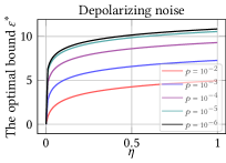
(a) The optimal bound function $\varepsilon^{*}(\eta)$ for hf_12.

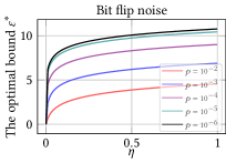
(b) The optimal bound function $\varepsilon^{*}(\eta)$ for hf_12.

Figure 7. Comparison of $\varepsilon$-differential privacy on Variational Quantum Eigensolver Algorithms with different noise levels.

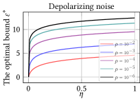
(a) The optimal bound function $\varepsilon^{*}(\eta)$ for QAOA_21.

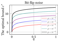
(b) The optimal bound function $\varepsilon^{*}(\eta)$ for QAOA_21.

Figure 8. Comparison of $\varepsilon$-differential privacy on Quantum Approximate Optimization Algorithms with different noise levels.

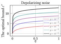
(a) The optimal bound function $\varepsilon^{*}(\eta)$ for inst_4x5_10.

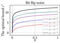
(b) The optimal bound function $\varepsilon^{*}(\eta)$ for inst_4x5_10.

Figure 9. Comparison of $\varepsilon$-differential privacy on Quantum Supremacy Algorithms with different noise levels.

(a) The optimal bound function $\varepsilon^{*}(\eta)$ for MNIST_10.

(b) The optimal bound function $\varepsilon^{*}(\eta)$ for GC_9.

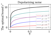
(c) The optimal bound function $\varepsilon^{*}(\eta)$ for EC_9.

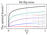
(d) The optimal bound function $\varepsilon^{*}(\eta)$ for MNIST_10.

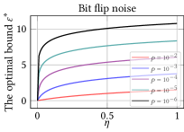
(e) The optimal bound function $\varepsilon^{*}(\eta)$ for GC_9.

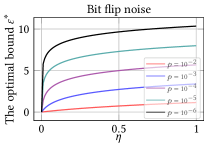
(f) The optimal bound function $\varepsilon^{*}(\eta)$ for EC_9.

Figure 10. Comparison of $\varepsilon$-differential privacy on various Quantum Machine Learning Models with different noise levels.

Optimal Bound Function $\varepsilon^{*}(\eta)$: After the above verification process, we have the values of $\kappa^{*}$ for all experiments. We choose the one in every kind of experiment with the largest qubits as the benchmark to depict the optimal bound function $\varepsilon^{*}(\eta)$ in Figs. 7-10, respectively. At the same time, we add more noise levels to further explore the tendency of the optimal bound function $\varepsilon^{*}(\eta)$. All experimental results confirm that the quantum noises on input states can logarithmically enhance the differential privacy as we claimed before. Furthermore, as quantum differential privacy protects the privacy of encoded classical data, as shown in Example 3.4, introducing quantum noise can further enhance the differential privacy of the encoded data, much like how adding classical noise improves the privacy of original classical data (dwork2014algorithmic, ).

6. Conclusion

In this paper, we established a formal framework for detecting violations of differential privacy for quantum algorithms. In particular, we developed an algorithm to not only verify whether or not a quantum algorithm is differentially private but also provide counterexamples when the privacy is unsatisfied. The counterexample consists of a pair of quantum states violating the privacy to reveal the cause of the violation. For practicability, we implemented our algorithm on TensorFlow Quantum and TorchQuantum, the quantum extensions of famous machine learning platforms — TensorFlow and PyTorch, respectively. Furthermore, for scalability, we adapted Tensor Networks (a highly efficient data structure) in our algorithm to overcome the state explosion (the complexity of the algorithm is exponential with the number of qubits) such that the practical performance of our algorithm can be improved. The effectiveness and efficiency of our algorithm were tested by numerical experiments on a bulk of quantum algorithms ranging from quantum supremacy (beyond classical computation) algorithms to quantum machine learning models with up to 21 qubits, which all have been implemented on current quantum hardware devices. The experimental results showed that quantum differential privacy can benefit from adding quantum noises on either quantum circuits or input states, which is consistent with the obtained theoretical results presented as Theorem 4.1.

For future works, extending the techniques developed for quantum algorithms in this paper to verify the differential privacy for quantum databases is an interesting research topic for protecting the privacy of quantum databases. As we discussed in Section 3, the neighboring relation for defining the differential privacy of quantum databases is the reachability between two quantum states by performing a quantum operation (super-operator) on a single quantum bit only (aaronson2019gentle, ), while that for our setting in this paper is the trace distance of two quantum states. Due to this fundamental difference in the neighboring relation, additional extensions will be required such as developing a reachability-based search algorithm to find the violations of the differential privacy for quantum databases. Another challenging research line is to study how to train a quantum machine learning algorithm with a differential privacy guarantee. This has been done for classical machine learning algorithms (abadi2016deep, ), but untouched at all for quantum algorithms.

Appendix

We begin with the proof of Theorem 4.1 as it will be used to prove the others.

Appendix A The Proof of Theorem 4.1

Proof.

For the first claim, by the definition of differential privacy in Definition 3.1, we have that for all quantum states $\rho,\sigma\in\mathcal{D(H)}$ with $D(\rho,\sigma)\leq\eta$ and $\mathcal{S}\subseteq\mathcal{O}$,

$$\sum_{k\in\mathcal{S}}{\rm tr}(M_{k}\mathcal{E}(\rho))\leq\exp(\varepsilon)\sum_{k\in\mathcal{S}}{\rm tr}(M_{k}\mathcal{E}(\sigma))+\delta$$

$$\Leftrightarrow{} \delta\geq\sum_{k\in\mathcal{S}}{\rm tr}(\mathcal{E}^{\dagger}(M_{k})(\rho-e^{\varepsilon}\sigma))$$

$$\Leftrightarrow{} \delta\geq{\rm tr}(M_{\mathcal{S}}(\rho-e^{\varepsilon}\sigma)).$$

By the arbitrariness of $\mathcal{S}$, the above inequality holds if and only if for any $\mathcal{S}\subseteq\mathcal{O}$, we have $\delta\geq\delta_{\mathcal{S}}$, where

(7) $$\delta_{\mathcal{S}}=\sup_{\rho,\sigma\text{ with }D(\rho,\sigma)\leq\eta}{\rm tr}(M_{\mathcal{S}}(\rho-e^{\varepsilon}\sigma)).$$

Next, we claim that

$$\delta_{\mathcal{S}}=\eta\lambda_{\max}(M_{\mathcal{S}})-(e^{\varepsilon}+\eta-1)\lambda_{\min}(M_{\mathcal{S}}).$$

First, let $\ket{\psi}$ and $\ket{\phi}$ be two normalized eigenvectors of $M_{\mathcal{S}}$ corresponding to the maximum and minimum eigenvalues, respectively, and

$$\gamma=\eta|\psi\rangle\langle\psi|+(1-\eta)|\phi\rangle\langle\phi|\qquad\phi=|\phi\rangle\langle\phi|.$$

Then, by the arbitrariness of $\rho,\sigma$ and $D(\gamma,\phi)=\eta$, we have that

$$\delta_{\mathcal{S}}\geq {\rm tr}(M_{\mathcal{S}}(\gamma-e^{\varepsilon}\phi))$$

$$= \eta{\rm tr}(M_{\mathcal{S}}\psi)+(1-\eta-e^{\varepsilon}){\rm tr}(M_{\mathcal{S}}\phi)$$

$$= \eta\lambda_{\max}(M_{\mathcal{S}})-(e^{\varepsilon}+\eta-1)\lambda_{\min}(M_{\mathcal{S}}).$$

On the other hand, for any quantum states $\rho,\sigma\in\mathcal{D(H)}$ with $D(\rho,\sigma)\leq\eta$, let $\rho-\sigma=\Delta_{+}-\Delta_{-}$ be a decomposition into orthogonal positive and negative parts (i.e., $\Delta_{\pm}\geq 0$ and $\Delta_{+}\Delta_{-}=0$). Then we have ${\rm tr}(\Delta_{+})={\rm tr}(\Delta_{-})$ because $0={\rm tr}(\rho-\sigma)={\rm tr}(\Delta_{+}-\Delta_{-})$, and then $\frac{1}{2}{\rm tr}(|\rho-\sigma|)={\rm tr}(\Delta_{+})$. Therefore, $D(\rho,\sigma)={\rm tr}(\Delta_{+})\leq\eta$. Furthermore,

$$\delta_{\mathcal{S}}= \sup_{\rho,\sigma\text{ with }D(\rho,\sigma)\leq\eta}{\rm tr}(M_{\mathcal{S}}(\rho-e^{\varepsilon}\sigma))$$

$$= \sup_{{\rm tr}(\Delta_{-})={\rm tr}(\Delta_{+})\leq\eta}{\rm tr}[M_{\mathcal{S}}(\Delta_{+}-\Delta_{-}+\sigma-e^{\varepsilon}\sigma)]$$

$$= \sup_{{\rm tr}(\Delta_{-})={\rm tr}(\Delta_{+})\leq\eta}{\rm tr}(M_{\mathcal{S}}\Delta_{+})-{\rm tr}(M_{\mathcal{S}}\Delta_{-})-(e^{\varepsilon}-1){\rm tr}(M_{\mathcal{S}}\sigma)$$

$$= \sup_{{\rm tr}(\Delta_{-})={\rm tr}(\Delta_{+})\leq\eta}{\rm tr}(\Delta_{+}){\rm tr}(M_{\mathcal{S}}\frac{\Delta_{+}}{{\rm tr}(\Delta_{+})})$$

$$-{\rm tr}(\Delta_{-}){\rm tr}(M_{\mathcal{S}}\frac{\Delta_{-}}{{\rm tr}(\Delta_{-})})-(e^{\varepsilon}-1){\rm tr}(M_{\mathcal{S}}\sigma)$$

$$\leq \sup_{{\rm tr}(\Delta_{-})={\rm tr}(\Delta_{+})\leq\eta}{\rm tr}(\Delta_{+})\max_{\rho_{1}\in\mathcal{D(H)}}{\rm tr}(M_{\mathcal{S}}\rho_{1})-{\rm tr}(\Delta_{-})\min_{\rho_{2}\in\mathcal{D(H)}}{\rm tr}(M_{\mathcal{S}}\rho_{2})-(e^{\varepsilon}-1)\min_{\rho_{3}\in\mathcal{D(H)}}{\rm tr}(M_{\mathcal{S}}\rho_{3})$$

$$= \sup_{{\rm tr}(\Delta_{-})={\rm tr}(\Delta_{+})\leq\eta}{\rm tr}(\Delta_{+})[\lambda_{\max}(M_{\mathcal{S}})-\lambda_{\min}(M_{\mathcal{S}})]-(e^{\varepsilon}-1)\lambda_{\min}(M_{\mathcal{S}})$$

$$\leq \eta\lambda_{\max}(M_{\mathcal{S}})-(e^{\varepsilon}+\eta-1)\lambda_{\min}(M_{\mathcal{S}}).$$

In summary, $\delta_{\mathcal{S}}=\eta\lambda_{\max}(M_{\mathcal{S}})-(e^{\varepsilon}+\eta-1)\lambda_{\min}(M_{\mathcal{S}})$. With this, we can complete the first claim in the theorem.

For proving the second one, we only need to set $\delta=0$ in the first claim and solve the inequalities $0\geq\delta_{\mathcal{S}}$ for any $\mathcal{S}\subseteq\mathcal{O}$. ∎

Appendix B The Proof of Theorem 3.5

Lemma B.1.

Let $\mathcal{E}$ be a super-operator on Hilbert space $\mathcal{H}$. Then for any positive semi-definite matrix $M$, we have

$$\lambda_{\min}(M)\leq\lambda_{\min}(\mathcal{E}^{\dagger}(M))\leq\lambda_{\max}(\mathcal{E}^{\dagger}(M))\leq\lambda_{\max}(M).$$

Proof.

First, we have that

$$\lambda_{\max}(M)=\max_{\rho\in\mathcal{D(H)}}{\rm tr}(M\rho)\text{ and }\lambda_{\min}(M)=\min_{\rho\in\mathcal{D(H)}}{\rm tr}(M\rho).$$

Thus,

$$\lambda_{\max}(\mathcal{E}^{\dagger}(M))=\max_{\rho\in\mathcal{D(H)}}{\rm tr}(\mathcal{E}^{\dagger}(M)\rho)$$

$$\lambda_{\min}(\mathcal{E}^{\dagger}(M))=\min_{\rho\in\mathcal{D(H)}}{\rm tr}(\mathcal{E}^{\dagger}(M)\rho).$$

Furthermore, as ${\rm tr}(\mathcal{E}^{\dagger}(M)\rho)={\rm tr}(M\mathcal{E}(\rho))$,

$$\lambda_{\max}(\mathcal{E}^{\dagger}(M))=\max_{\rho\in\mathcal{D(H)}}{\rm tr}(M\mathcal{E}(\rho))$$

$$\lambda_{\min}(\mathcal{E}^{\dagger}(M))=\min_{\rho\in\mathcal{D(H)}}{\rm tr}(M\mathcal{E}(\rho)).$$

Let $\mathcal{S}=\{\mathcal{E}(\rho)|\rho\in\mathcal{D(H)}\}$. Then

$$\lambda_{\max}(\mathcal{E}^{\dagger}(M))=\max_{\rho\in\mathcal{S}}{\rm tr}(M\rho)\text{ and }\lambda_{\min}(\mathcal{E}^{\dagger}(M))=\min_{\rho\in\mathcal{S}}{\rm tr}(M\rho).$$

Because of $\mathcal{S}\subseteq\mathcal{D(H)}$, we obtain that $\lambda_{\min}(M)\leq\lambda_{\min}(\mathcal{E}^{\dagger}(M))$ and $\lambda_{\max}(\mathcal{E}^{\dagger}(M))\leq\lambda_{\max}(M)$, completing the proof. ∎

Now we can prove Theorem 3.5.

Proof.

It follows from Theorem 4.1 and Lemma B.1 by noting that $\lambda_{\max}(\mathcal{U}^{\dagger}(M))=\lambda_{\max}(M)$ and $\lambda_{\min}(\mathcal{U}^{\dagger}(M))=\lambda_{\min}(M)$ for any positive semi-definite matrix $M$. ∎

Appendix C The Proof of Theorem 3.6

Proof.

First, we prove Claim 1. For $k\in\{1,2\},$ we redefine ${M}_{k,\mathcal{S}_{k}}=\sum_{j_{k}\in\mathcal{S}_{k}}\mathcal{E}_{k}^{\dagger}(M_{k,j_{k}})$. Then by Theorem 4.1,

$$\max_{\mathcal{S}_{1}\subseteq\mathcal{O}_{1}}\kappa(M_{1,\mathcal{S}_{1}})\leq\frac{e^{\varepsilon_{1}}+\eta_{1}-1}{\eta_{1}}\qquad\max_{\mathcal{S}_{2}\subseteq\mathcal{O}_{1}}\kappa(M_{2,\mathcal{S}_{2}})\leq\frac{e^{\varepsilon_{2}}+\eta_{2}-1}{\eta_{2}}.$$

With the above two inequalities, we have

$$\max_{\mathcal{S}_{1}\subseteq\mathcal{O}_{1}}\max_{\mathcal{S}_{2}\subseteq\mathcal{O}_{2}}\kappa(M_{1,\mathcal{S}_{1}})\kappa(M_{2,\mathcal{S}_{2}})$$

$$\leq \frac{e^{\varepsilon_{1}}+\eta_{1}-1}{\eta_{1}}\frac{e^{\varepsilon_{2}}+\eta_{2}-1}{\eta_{2}}$$

$$= \frac{e^{\varepsilon_{1}+\varepsilon_{2}}+(\eta_{1}-1)(\eta_{2}-1)+e^{\varepsilon_{1}}(\eta_{2}-1)+e^{\varepsilon_{2}}(\eta_{1}-1)}{\eta_{1}\eta_{2}}$$

$$\leq \frac{e^{\varepsilon_{1}+\varepsilon_{2}}+(\eta_{1}-1)(\eta_{2}-1)+\eta_{1}+\eta_{2}-2}{\eta_{1}\eta_{2}}$$

$$= \frac{e^{\varepsilon_{1}+\varepsilon_{2}}+\eta_{1}\eta_{2}-1}{\eta_{1}\eta_{2}}.$$

The last inequality results from $e^{\varepsilon}\geq 1$ for any $\varepsilon\geq 0$ and $\eta_{1},\eta_{2}\leq 1$.

Next, we prove Claim 2.

For any subsets $\mathcal{S}_{1}\subseteq\mathcal{O}_{1}$ and $\mathcal{S}_{2}\subseteq\mathcal{O}_{2}$, we have

$$\eta_{1}\eta_{2}\lambda_{\max}(M_{1,\mathcal{S}_{1}}\otimes M_{2,\mathcal{S}_{2}})-(e^{\varepsilon_{1}+\varepsilon_{2}}+\eta_{1}\eta_{2}-1)\lambda_{\min}(M_{1,\mathcal{S}_{1}}\otimes M_{2,\mathcal{S}_{2}})$$

$$= \eta_{1}\eta_{2}\lambda_{\max}(M_{1,\mathcal{S}_{1}})\lambda_{\max}(M_{2,\mathcal{S}_{2}})-(e^{\varepsilon_{1}+\varepsilon_{2}}+\eta_{1}\eta_{2}-1)\lambda_{\min}(M_{1,\mathcal{S}_{1}})\lambda_{\min}(M_{2,\mathcal{S}_{2}})$$

$$\leq \eta_{1}\eta_{2}\lambda_{\max}(M_{1,\mathcal{S}_{1}})\lambda_{\max}(M_{2,\mathcal{S}_{2}})-(e^{\varepsilon_{1}}+\eta_{1}-1)(e^{\varepsilon_{2}}+\eta_{2}-1)\lambda_{\min}(M_{1,\mathcal{S}_{1}})\lambda_{\min}(M_{2,\mathcal{S}_{2}})$$

$$\leq \eta_{1}\eta_{2}\lambda_{\max}(M_{1,\mathcal{S}_{1}})\lambda_{\max}(M_{2,\mathcal{S}_{2}})-(\eta_{1}\lambda_{\max}(M_{1,\mathcal{S}_{1}})-\delta_{1})(\eta_{2}\lambda_{\max}(M_{2,\mathcal{S}_{2}})-\delta_{2})$$

$$= \eta_{1}\lambda_{\max}(M_{1,\mathcal{S}_{1}})\delta_{2}+\eta_{2}\lambda_{\max}(M_{2,\mathcal{S}_{2}})\delta_{1}-\delta_{1}\delta_{2}$$

$$\leq \delta_{1}+\delta_{2}.$$

The first inequality results from $(e^{\varepsilon_{1}+\varepsilon_{2}}+\eta_{1}\eta_{2}-1)\geq(e^{\varepsilon_{1}}+\eta_{1}-1)(e^{\varepsilon_{2}}+\eta_{2}-1)$, the second one follows from Theorem 4.1, and the last one comes from the fact that $0\leq\eta_{1},\eta_{2},\lambda_{\max}(M_{1,\mathcal{S}_{1}}),\lambda_{\max}(M_{2,\mathcal{S}_{2}})\leq 1$. ∎

Appendix D The Proof of Theorem 4.2

Proof.

It follows from the proof of Theorem 4.1 that $\delta_{\mathcal{S}}$ defined by Eq. (7) can be reached by the following pair of quantum states:

$$(\eta|\psi\rangle\langle\psi|+(1-\eta)|\phi\rangle\langle\phi|),|\phi\rangle\langle\phi|)$$

for any normalized eigenvectors $\ket{\psi}$ and $\ket{\phi}$ of $M_{\mathcal{S}}$ corresponding to the maximum and minimum eigenvalues, respectively. ∎

References

- [1] Lov K Grover. A fast quantum mechanical algorithm for database search. In Proceedings of the twenty-eighth annual ACM symposium on Theory of computing, pages 212–219, 1996.
- [2] Peter W Shor. Algorithms for quantum computation: discrete logarithms and factoring. In Proceedings 35th annual symposium on foundations of computer science, pages 124–134. Ieee, 1994.
- [3] Aram W Harrow, Avinatan Hassidim, and Seth Lloyd. Quantum algorithm for linear systems of equations. Physical review letters, 103(15):150502, 2009.
- [4] Patrick Rebentrost, Masoud Mohseni, and Seth Lloyd. Quantum support vector machine for big data classification. Physical Review Letters, 113(3):1–5, 2014.
- [5] Iris Cong, Soonwon Choi, and Mikhail D Lukin. Quantum convolutional neural networks. Nature Physics, 15(12):1273–1278, 2019.
- [6] Johannes Bausch. Recurrent quantum neural networks. Advances in neural information processing systems, 33:1368–1379, 2020.
- [7] Pierre-Luc Dallaire-Demers and Nathan Killoran. Quantum generative adversarial networks. Physical Review A, 98(1):012324, 2018.
- [8] Daoyi Dong, Chunlin Chen, Hanxiong Li, and Tzyh-Jong Tarn. Quantum reinforcement learning. IEEE Transactions on Systems, Man, and Cybernetics, Part B (Cybernetics), 38(5):1207–1220, 2008.
- [9] Nana Liu and Patrick Rebentrost. Quantum machine learning for quantum anomaly detection. Physical Review A, 97(4):042315, 2018.
- [10] Alessandra Di Pierro and Massimiliano Incudini. Quantum machine learning and fraud detection. In Protocols, Strands, and Logic, pages 139–155. Springer, 2021.
- [11] Ricardo García, Jordi Cahue, and Santiago Pavas. Credit risk scoring with a supervised quantum classifier. 05 2020.
- [12] Andrew Milne, Maxwell Rounds, and Phil Goddard. Optimal feature selection in credit scoring and classification using a quantum annealer. White Paper 1Qbit, 2017.
- [13] Google. Tensorflow Quantum, https://www.tensorflow.org/quantum, Accessed 2021.
- [14] Edward Farhi, Jeffrey Goldstone, and Sam Gutmann. A quantum approximate optimization algorithm. arXiv preprint arXiv:1411.4028, 2014.
- [15] Alberto Peruzzo, Jarrod McClean, Peter Shadbolt, Man-Hong Yung, Xiao-Qi Zhou, Peter J Love, Alán Aspuru-Guzik, and Jeremy L O’brien. A variational eigenvalue solver on a photonic quantum processor. Nature communications, 5(1):4213, 2014.
- [16] Hanrui Wang, Yongshan Ding, Jiaqi Gu, Yujun Lin, David Z Pan, Frederic T Chong, and Song Han. Quantumnas: Noise-adaptive search for robust quantum circuits. In 2022 IEEE International Symposium on High-Performance Computer Architecture (HPCA), pages 692–708. IEEE, 2022.
- [17] Google AI Quantum, Collaborators*†, Frank Arute, Kunal Arya, Ryan Babbush, Dave Bacon, Joseph C Bardin, Rami Barends, Sergio Boixo, Michael Broughton, Bob B Buckley, et al. Hartree-fock on a superconducting qubit quantum computer. Science, 369(6507):1084–1089, 2020.
- [18] Matthew P Harrigan, Kevin J Sung, Matthew Neeley, Kevin J Satzinger, Frank Arute, Kunal Arya, Juan Atalaya, Joseph C Bardin, Rami Barends, Sergio Boixo, et al. Quantum approximate optimization of non-planar graph problems on a planar superconducting processor. Nature Physics, 17(3):332–336, 2021.
- [19] Frank Arute, Kunal Arya, Ryan Babbush, Dave Bacon, Joseph C Bardin, Rami Barends, Rupak Biswas, Sergio Boixo, Fernando GSL Brandao, David A Buell, et al. Quantum supremacy using a programmable superconducting processor. Nature, 574(7779):505–510, 2019.
- [20] Han-Sen Zhong, Hui Wang, Yu-Hao Deng, Ming-Cheng Chen, Li-Chao Peng, Yi-Han Luo, Jian Qin, Dian Wu, Xing Ding, Yi Hu, et al. Quantum computational advantage using photons. Science, 370(6523):1460–1463, 2020.
- [21] Cynthia Dwork, Aaron Roth, et al. The algorithmic foundations of differential privacy. Foundations and Trends® in Theoretical Computer Science, 9(3–4):211–407, 2014.
- [22] Zhanglong Ji, Zachary C Lipton, and Charles Elkan. Differential privacy and machine learning: a survey and review. arXiv preprint arXiv:1412.7584, 2014.
- [23] Gilles Barthe, George Danezis, Benjamin Grégoire, César Kunz, and Santiago Zanella-Beguelin. Verified computational differential privacy with applications to smart metering. In 2013 IEEE 26th Computer Security Foundations Symposium, pages 287–301. IEEE, 2013.
- [24] Gilles Barthe, Noémie Fong, Marco Gaboardi, Benjamin Grégoire, Justin Hsu, and Pierre-Yves Strub. Advanced probabilistic couplings for differential privacy. In Proceedings of the 2016 ACM SIGSAC Conference on Computer and Communications Security, pages 55–67, 2016.
- [25] Gilles Barthe, Marco Gaboardi, Emilio Jesús Gallego Arias, Justin Hsu, César Kunz, and Pierre-Yves Strub. Proving differential privacy in hoare logic. In 2014 IEEE 27th Computer Security Foundations Symposium, pages 411–424. IEEE, 2014.
- [26] Gilles Barthe, Marco Gaboardi, Benjamin Grégoire, Justin Hsu, and Pierre-Yves Strub. Proving differential privacy via probabilistic couplings. In Proceedings of the 31st Annual ACM/IEEE Symposium on Logic in Computer Science, pages 749–758, 2016.
- [27] Gilles Barthe, Boris Köpf, Federico Olmedo, and Santiago Zanella Beguelin. Probabilistic relational reasoning for differential privacy. In Proceedings of the 39th annual ACM SIGPLAN-SIGACT symposium on Principles of programming languages, pages 97–110, 2012.
- [28] Gilles Barthe and Federico Olmedo. Beyond differential privacy: Composition theorems and relational logic for f-divergences between probabilistic programs. In Automata, Languages, and Programming: 40th International Colloquium, ICALP 2013, Riga, Latvia, July 8-12, 2013, Proceedings, Part II 40, pages 49–60. Springer, 2013.
- [29] Zeyu Ding, Yuxin Wang, Guanhong Wang, Danfeng Zhang, and Daniel Kifer. Detecting violations of differential privacy. In Proceedings of the 2018 ACM SIGSAC Conference on Computer and Communications Security, pages 475–489, 2018.
- [30] Li Zhou and Mingsheng Ying. Differential privacy in quantum computation. In 2017 IEEE 30th Computer Security Foundations Symposium (CSF), pages 249–262. IEEE, 2017.
- [31] Scott Aaronson and Guy N Rothblum. Gentle measurement of quantum states and differential privacy. In Proceedings of the 51st Annual ACM SIGACT Symposium on Theory of Computing, pages 322–333, 2019.
- [32] Christoph Hirche, Cambyse Rouzé, and Daniel Stilck Franca. Quantum differential privacy: An information theory perspective. arXiv preprint arXiv:2202.10717, 2022.
- [33] Michael A Nielsen and Isaac L Chuang. Quantum computation and quantum information. Cambridge university press, 2010.
- [34] Armando Angrisani, Mina Doosti, and Elham Kashefi. Differential privacy amplification in quantum and quantum-inspired algorithms. arXiv preprint arXiv:2203.03604, 2022.
- [35] Ji Guan, Wang Fang, and Mingsheng Ying. Robustness verification of quantum classifiers. In International Conference on Computer Aided Verification, pages 151–174. Springer, 2021.
- [36] Yuxuan Du, Min-Hsiu Hsieh, Tongliang Liu, Dacheng Tao, and Nana Liu. Quantum noise protects quantum classifiers against adversaries. Physical Review Research, 3(2):023153, 2021.
- [37] Rafael Pinot, Florian Yger, Cédric Gouy-Pailler, and Jamal Atif. A unified view on differential privacy and robustness to adversarial examples. arXiv preprint arXiv:1906.07982, 2019.
- [38] Desmond J Higham. Condition numbers and their condition numbers. Linear Algebra and its Applications, 214:193–213, 1995.
- [39] Michael M Wolf. Quantum channels & operations: Guided tour. Lecture notes available at https://www-m5.ma.tum.de/foswiki/pub/M5/Allgemeines/MichaelWolf/QChannelLecture.pdf, 2012.
- [40] Zhaojun Bai, James Demmel, Jack Dongarra, Axel Ruhe, and Henk van der Vorst. Templates for the Solution of Algebraic Eigenvalue Problems. Society for Industrial and Applied Mathematics, 2000.
- [41] Aws Albarghouthi et al. Introduction to neural network verification. Foundations and Trends® in Programming Languages, 7(1–2):1–157, 2021.
- [42] Yizhak Yisrael Elboher, Justin Gottschlich, and Guy Katz. An abstraction-based framework for neural network verification. In International Conference on Computer Aided Verification, pages 43–65. Springer, 2020.
- [43] Nengkun Yu and Jens Palsberg. Quantum abstract interpretation. In Proceedings of the 42nd ACM SIGPLAN International Conference on Programming Language Design and Implementation, pages 542–558, 2021.
- [44] Wang Lin, Zhengfeng Yang, Xin Chen, Qingye Zhao, Xiangkun Li, Zhiming Liu, and Jifeng He. Robustness verification of classification deep neural networks via linear programming. In Proceedings of the IEEE/CVF Conference on Computer Vision and Pattern Recognition, pages 11418–11427, 2019.
- [45] Igor L Markov and Yaoyun Shi. Simulating quantum computation by contracting tensor networks. SIAM Journal on Computing, 38(3):963–981, 2008.
- [46] Jacob C Bridgeman and Christopher T Chubb. Hand-waving and interpretive dance: an introductory course on tensor networks. Journal of physics A: Mathematical and theoretical, 50(22):223001, 2017.
- [47] Quantum AI team and collaborators. Recirq, October 2020.
- [48] Sergio Boixo, Sergei V Isakov, Vadim N Smelyanskiy, Ryan Babbush, Nan Ding, Zhang Jiang, Michael J Bremner, John M Martinis, and Hartmut Neven. Characterizing quantum supremacy in near-term devices. Nature Physics, 14(6):595–600, 2018.
- [49] Ji Guan, Wang Fang, and Mingsheng Ying. Verifying fairness in quantum machine learning. In Computer Aided Verification: 34th International Conference, CAV 2022, Haifa, Israel, August 7–10, 2022, Proceedings, Part II, pages 408–429. Springer, 2022.
- [50] Dheeru Dua and Casey Graff. UCI machine learning repository, 2017.
- [51] Ramaravind K. Mothilal, Amit Sharma, and Chenhao Tan. Explaining machine learning classifiers through diverse counterfactual explanations. Proceedings of the 2020 Conference on Fairness, Accountability, and Transparency, Jan 2020.
- [52] Machine Learning Group ULB. Credit card fraud detection. https://www.kaggle.com/datasets/mlg-ulb/creditcardfraud, 2018.
- [53] Yann LeCun and Corinna Cortes. MNIST handwritten digit database. http://yann.lecun.com/exdb/mnist/, 2010.
- [54] Han Xiao, Kashif Rasul, and Roland Vollgraf. Fashion-mnist: a novel image dataset for benchmarking machine learning algorithms, 2017.
- [55] Martin Abadi, Andy Chu, Ian Goodfellow, H Brendan McMahan, Ilya Mironov, Kunal Talwar, and Li Zhang. Deep learning with differential privacy. In Proceedings of the 2016 ACM SIGSAC conference on computer and communications security, pages 308–318, 2016.