ABC Easy as 123: A Blind Counter for Exemplar-Free
Multi-Class Class-agnostic Counting

Abstract

Class-agnostic counting methods enumerate objects of an arbitrary class, providing tremendous utility in many fields. Prior works have limited usefulness as they require either a set of examples of the type to be counted or that the image contains only a single type of object. A significant factor in these shortcomings is the lack of a dataset to properly address counting in settings with more than one kind of object present. To address these issues, we propose the first Multi-class, Class-Agnostic Counting dataset (MCAC) and A Blind Counter (ABC123), a method that can count multiple types of objects simultaneously without using examples of type during training or inference. ABC123 introduces a new paradigm where instead of requiring exemplars to guide the enumeration, examples are found after the counting stage to help a user understand the generated outputs. We show that ABC123 outperforms contemporary methods on MCAC without the requirement of human in-the-loop annotations. We also show that this performance transfers to FSC-147, the standard class-agnostic counting dataset. Project page: ABC123.active.vision

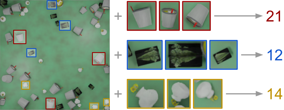
(a) Exemplar-Based Counting

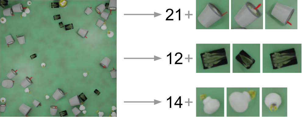
(b) Our Exemplar-Free Counting

Figure 1: ABC123 counts objects of multiple unseen types. Our method not only does not need exemplars to define the type to count but also finds examples of each type it has counted.

1 Introduction

Given an image and told to ‘count’, a person would generally understand the intended task and complete it with accuracy even if the kind of objects present has not been previously observed. However, in cases with a large number of objects, this is likely very slow.

This natural human ability to count arbitrarily has not been modelled by today’s datasets or methods. Current automated methods can count with a fair level of accuracy, so long as they have either an exemplar image as a prior on the type to count or an image with only one class of object.

Since real-world situations will likely include objects of multiple classes, methods need to accurately count in these environments. We first introduce MCAC, a new synthetic multi-class class-agnostic counting dataset, and show that methods previously assumed to work in multi-class settings perform poorly on it. We then propose ABC123, a multi-class class-agnostic counter which does not need exemplars during training or inference. ABC123 significantly outperforms prior works on MCAC while also generalising to other datasets, mirroring the arbitrary nature of human counting abilities.

Our contributions are:

• We introduced MCAC, the first multi-class class-agnostic counting dataset

• We propose ABC123, the first exemplar-free multi-class class-agnostic counter

• We show that prior methods do not perform as expected in multi-class settings and that ABC123 tackles multi-class counting effectively

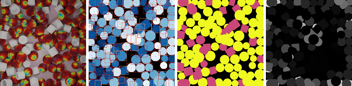
Figure 2: An example image from the training set of MCAC. All objects have associated instance labels, class labels, bounding boxes, centre points, and occlusion percentages.

2 Related Work

Class-specific counting methods aim to enumerate the instances of a single or small set of known classes [1, 5, 8, 23]. These methods struggle to adapt to novel classes and need new data and retraining for each type of object. To address these issues, Lu et al. [12] proposed class-agnostic counting, a framework without inference-time classes during training. Still most class-agnostic methods [16, 25, 19], including this one, require an exemplar images of the object class at test time. These methods generally work by creating a sufficiently general feature space and applying some form of matching to the whole feature map [25, 18] or to proposed regions of interest [16, 19].

Recent works, RepRPN [15], CounTR [11], ZSC [24] and RCC [6] do away with exemplar images at inference-time, removing the need for intervention during deployment. RepRPN is a two-step method which proposes regions likely to contain an object of interest and then uses them for an exemplar-based density map regression method. It proposes more than one bounding box and enumerates them separately. ZSC [24] uses a multi-stage process in which a text input is used to generate an generic image of the type to be counted that is then used to find exemplar patches. These exemplar patches then function as the input to an exemplar-based method [18]. CounTR uses a large vision-transformer encoder-decoder to regress a density map of instance locations. It is trained in a mixed few/zero-shot way, applying understanding gained from exemplar-based examples to exemplar-free cases.

It has been assumed that the above methods can function in multi-class settings. However, this has not been proven rigorously because the main dataset for class-agnostic counting (FSC-147/133 [16, 6]) contains only one labelled class per image. In fact, we show in Sec. 5 that these methods perform poorly in contexts with multiple types present. FSC-147 being single-class has also explicitly motivated work such as RCC, which regresses a single scalar value from an image. It is trained without exemplar images and uses only scalar supervision instead of density maps. Even with the constraint of only counting one kind of object and with no further direction on the type to count, RCC achieves competitive results with exemplar-based methods on FSC-147, showing the limitations of this dataset.

While large models with image inputs [14] like SAM [9] would seem to be able to effectively count objects of arbitrary types, in fact these methods have poor numerical understanding [13], and SAM performs unsatisfactorily on all counting tasks but especially on images with small objects or a high density of objects.

3 MCAC Dataset

3.1 Motivation

There are currently no datasets suitable for multi-class class-agnostic counting problems. This significantly impacts the research into methods addressing these tasks. The use of FSC-147 as the main class-agnostic counting dataset has caused many problems, the lack of multi-class cases being one of the most significant. This has lead to many methods being wrongly assumed to work in multi-class settings. It has also limited the development of exemplar-free multi-class methods. To this end we introduce MCAC, the first multi-class class-agnostic counting dataset.

While the deployment query scenario, counting given an unlabelled image of objects, is natural, the training and quantitative evaluation of methods to address it is not. To facilitate training and evaluation of methods in multi-class settings, we need images with multiple objects of multiple types. To evaluate a methods generalisability to unseen object types, the classes present in the images need to be mutually exclusive between training, validation and testing. It is infeasible to gather natural images with (a) a wide variety of classes, (b) a wide variety of the number of times an object appears in an image, and (c) no repetition of the types of object between the train, test, and validation splits. Using synthetic images allows the above constraints to be satisfied while also providing a high level of precision and accuracy in the labels for each image. As shown in Sec. 5.3, the understanding gained from training on synthetic data is general enough to apply to the standard photographic counting dataset, FSC [16].

3.2 Ambiguity

Both exemplar-based and exemplar-free methods bump into problems of ambiguity. If there are objects of varied levels of generality, which boundary should be used? For example, on a chess board with a single white pawn as the exemplar, should the count be of all the pieces, all the white pieces, all the white pawns, all the pawns, and so on?

Given the infeasability of defining every possible way of grouping the objects present in an image, we define a single way of grouping the objects: an identical mesh and texture, independent of size or orientation. We do, however, acknowledge the existence of other valid-but-unknown counts, the unlabelled ways of grouping the objects.

3.3 Dataset

MCAC contains images with between 1 and 4 classes of object and between 1 and 400 instances per class. The distribution of classes per image and instances per class are shown in Fig. 3. MCAC has three data splits: training with 4756 images (8298 counts) drawn from 287 classes; validation 2413 images (3640 counts) drawn from 37 classes, and testing with 2114 images (4286 counts) drawn from 19 classes. Each instances in an image have associated class labels, model labels, center coordinates, bounding box coordinates, segmentation maps, unoccluded segmentation maps, and occlusion percentages. The occlusion percentage is calculated as $1-\frac{A_{0}}{A_{1}}$, where $A_{0}$ is the number of pixels in the final image and $A_{1}$ is the number of pixels that would be seen if the object was unoccluded and was completely within the bounds of the image.

Objects are ‘dropped’ into the scene, ensuring random locations and orientations. As objects in real setting often vary in size, we vary the size of objects by $\pm$50% from a random nominal size. We also vary the number, location, and intensity of lights present. Models and textures are drawn from ShapeNetSem [17]. The exact data splits by class name are in Appendix A.

Number of Classes

(a) *

Number of Instances

(b) *

Figure 3: Distributions of the number of classes in an image and of the number of instances of each class per image across the dataset.

3.4 Using MCAC

Here we lay out our suggested usage of MCAC, which we used to generate our results. We will also release code for a pytorch dataset to enable easy adoption.

Objects that are more than 70% occluded by either other objects or the edge of the frame should be excluded. The ground-truth density map has a Gaussian centred on the center pixel of each object with $\sigma=8$. As is standard [16, 11, 25, 10], when the Gaussians from different instances overlap, we sum them rather than taking the maximum value. We then scale the whole density map so the sum over it is the correct value. This adjustment improved our results by $\sim 5\%$.

When training exemplar-based methods, we take bounding boxes randomly from instances with less than 30% occlusion. We evaluate these methods using the bounding boxes of the three least occluded instances. In cases with more than three equally occluded instances, we use those with the lowest instance IDs.

4 Method

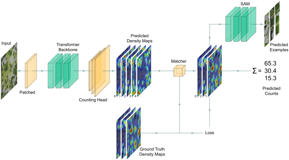
Figure 4: The ABC123 pipeline. Our method learns to count objects of multiple novel classes without needing exemplar images. During training and quantitative evaluation, the matcher aligns the unguided predictions to the ground truth labels. The example prediction stage locates instances associated with each generated count.

Our method, ABC123, takes an image with multiple instances of objects of multiple types and regresses the count of each type. This is achieved blind, i.e. on objects of arbitrary classes with no requirement to have seen the object class during training or to have an exemplar image to define the type during inference. We achieve this by first regressing density maps for each type then enumerating the instances using integration. To facilitate training and evaluating ABC123 in an exemplar-free way, we propose a matching stage. To further increase the interpretability of the outputs of ABC123, we design an example discovery stage which finds specific instances of the counted object.

4.1 Density Map Regression

For each image, there are $m$ classes present, each with an associated ground truth count $y$ and density map $d$. We regress $\hat{m}$ counts and density map predictions, $\hat{y}$ and $\hat{d}$ respectively.

$$\hat{y}=\sum_{h,w}{\hat{d}_{(h,w)}}$$ (1)

where $\hat{d}_{(h,w)}$ denotes the density value for pixel (h, w). We achieve this by using $\hat{m}$ convolutional up-sampling heads on top of a vision transformer backbone [4]. We use a vision transformer backbone due to its globally receptive field and self-attention mechanism, which Hobley and Prisacariu [6] showed is crucial to generating a complex understanding in counting settings. Each head regresses a single pixel-wise density map prediction and count prediction from a patch-wise low-resolution high-dimensional feature space.

Similar to other contemporary methods [16, 11, 25, 10], we use the pixel-wise error $||d-\hat{d}||_{1}$ as our loss, where $d$ and $\hat{d}$ are the ground truth and predicted density maps. This produced more accurate results than using the L₂ distance between the $d$ and $\hat{d}$; see Sec. 6.1 for the full comparison.

4.2 Matching

In single-class or exemplar-based settings, there is a single prediction-label pair. However, in multi-class exemplar-free settings, there are multiple predictions as well as multiple labels, without a clearly defined pairing. This resembles class-discovery [21, 26] and clustering [7, 22] problems, where the number and cardinality of new classes is not necessarily known.

In keeping with these fields and to facilitate training and evaluate accuracy, we find correspondences between the set of $m$ known counts and the set of $\hat{m}$ predicted counts. The correspondence matrix is defined as $\mathcal{X}=\{0,1\}^{m\times\hat{m}}$ where $\mathcal{X}_{i,j}=1$ iff prediction $i$ is assigned to label $j$. A problem instance is described by an $m\times\hat{m}$ cost matrix $\mathcal{C}$, where $\mathcal{C}_{i,j}$ is the cost of matching prediction $i$ and ground truth label $j$. The goal is to find the complete assignment of predictions to labels of minimal cost. Formally, the optimal assignment has cost

$$\min_{\mathcal{X}}\sum_{i=0}^{m}\sum_{j=0}^{\hat{m}}\mathcal{C}_{i,j}\cdot\mathcal{X}_{i,j}$$ (2)

Specifically, our cost function is defined as the the pixel-wise distance of the normalised ground truth density map $d_{i}$ and the predicted density map $\hat{d}_{j}$.

$$\mathcal{C}_{i,j}=\left|\left|\frac{d_{i}}{||d_{i}||_{2}}-\frac{\hat{d}_{j}}{||\hat{d}_{j}||_{2}}\right|\right|_{2}$$ (3)

The normalisation ensures the matching is done on the locality of the counted objects rather than the magnitude of the prediction itself. We use the Hungarian algorithm, specifically the Jonker-Volgenant algorithm outlined in Crouse [3], to solve for $\mathcal{X}$ robustly.

The supervision loss for each image is the sum of the L₁ difference of the ground truth density maps and their matched predictions as:

$$\mathcal{L}=\sum_{i,j}^{m,\hat{m}}||d_{i}-\hat{d}_{j}||_{1}\cdot\mathcal{X}_{i,j}$$ (4)

It should be noted that every label has an associated prediction, but the inverse is not the case as generally $\hat{m}>m$. This means we do not impose a loss on the unmatched density maps. This allows the network to generate more nuanced count definitions as it does not punish valid-but-unknown counts which are likely present in any counting setting.

As is usual [21, 26, 7, 22], we use the same matching procedure to evaluate our performance at inference-time. It should be noted that as this matching uses the ground-truth density maps, it could be used to significantly benefit a method’s quantitative results without improving its deployment capabilities. Specifically, a method could in principle predict all possible density maps and use the matching stage to pick the correct one. We limit ourselves to generating 5 density maps to minimise this behaviour. We explore the effect of this further in Sec. 6.3. We also normalise the density maps between 0 and 1 to ensure we are only matching to the locations of objects rather than the counts themselves.

4.3 Example Discovery

While exemplar-free counting saves a user time, as no manual intervention is required, it does require the user to interpret the results. A set of scalar count values can be unclear as it is not always obvious which count corresponds to which type of object in the input image. Density maps can also often be difficult to interpret, especially in high density situations.

To aid the user in understanding to which class a generated count corresponds, we propose flipping the usual exemplar-based paradigm. Instead of using exemplar images to define the type to count, we find examples of the type counted. We achieve this by using the peaks from the predicted density map as seed inputs for a pre-trained segmentation method [9]. While this segmentation method is often not accurate enough to segment a singular whole object given only a singular point, they are generally good enough that an expanded bounding box around them contains enough information for a user to understand the class of object that has been counted; see Fig. 7 for examples.

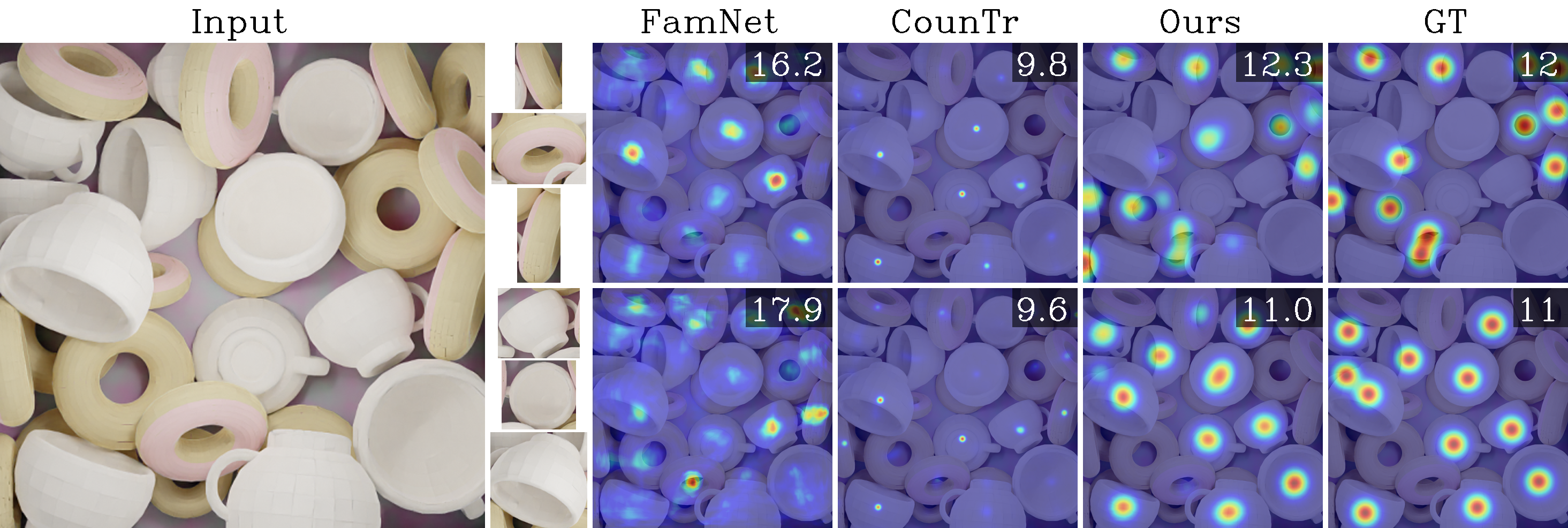
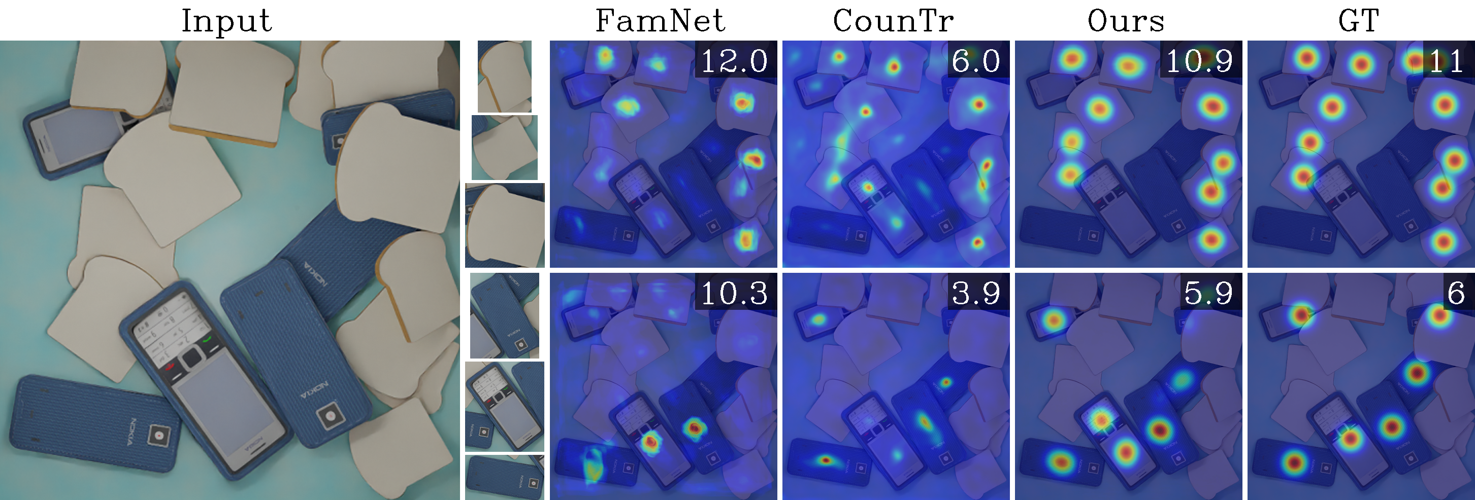
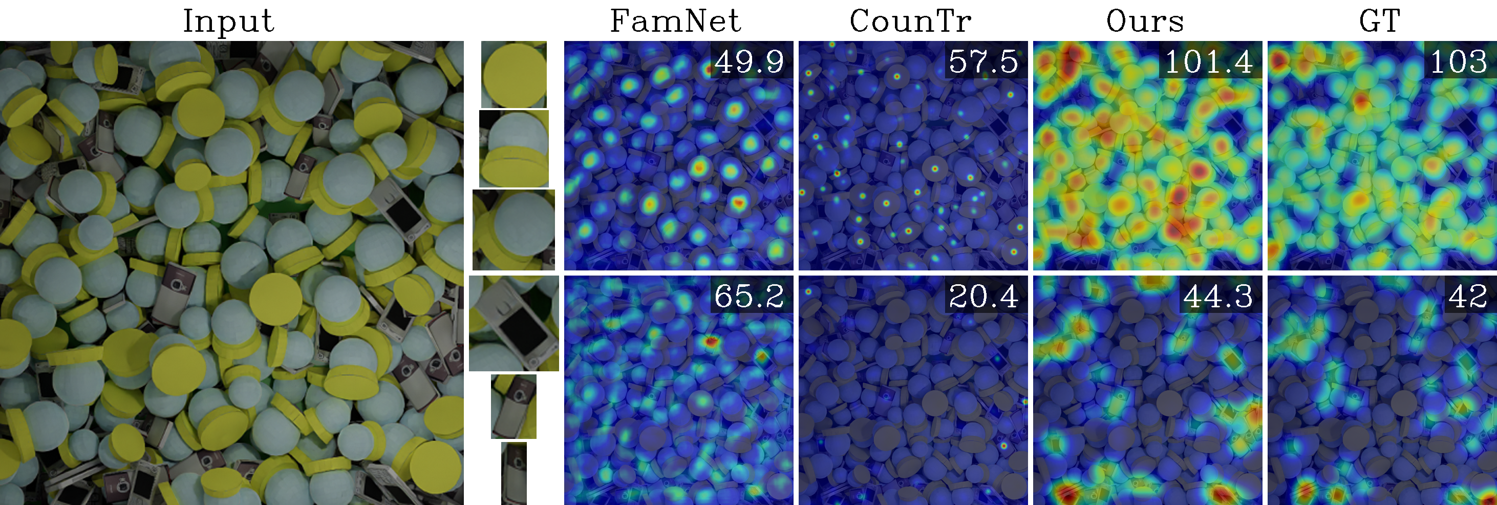
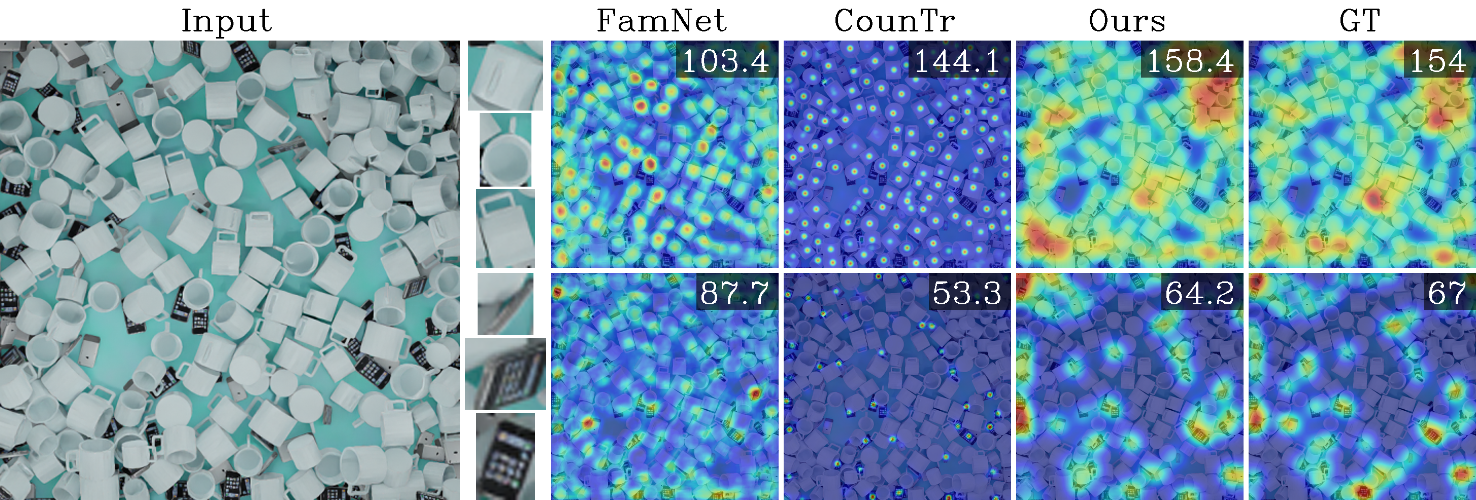
Figure 5: Comparison to other methods on MCAC. ABC123 produces more accurate results than the exemplar-based methods without using exemplar images. The ground truth (GT) and predicted counts are shown in the top right corner of their respective density maps.

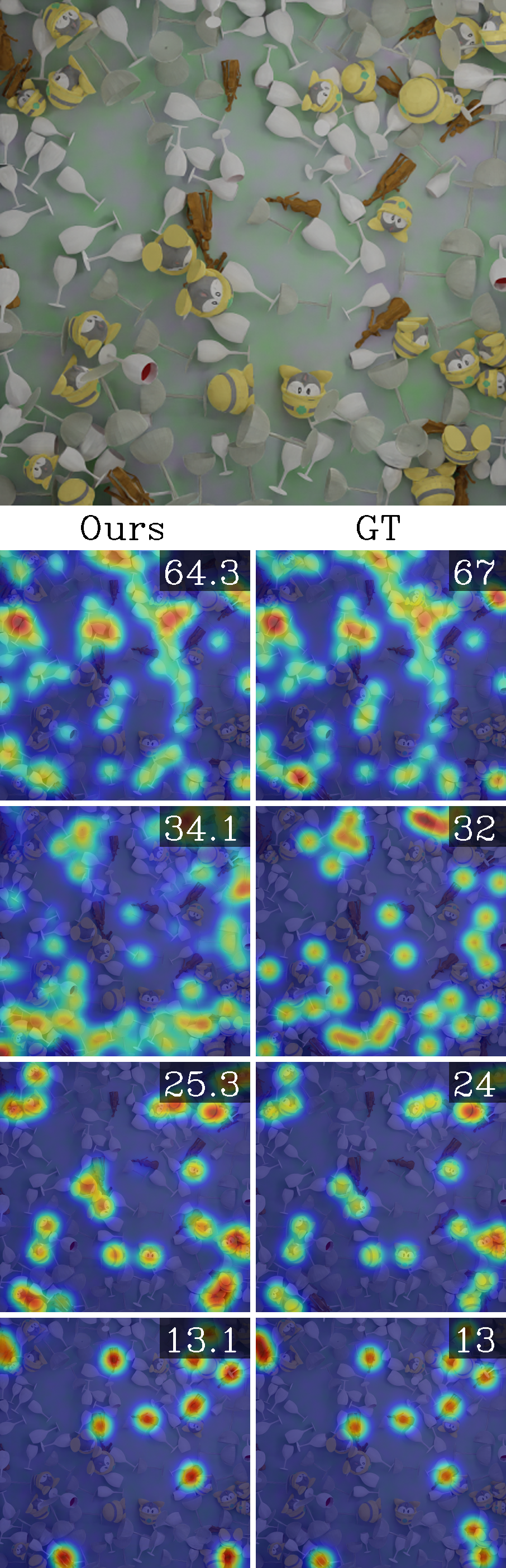
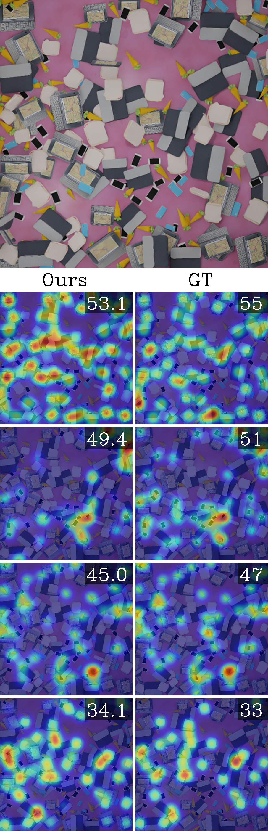
Figure 6: Results of our method on images with 4 classes. ABC123 is able to generate accurate counts and meaningful density maps from images with four novel classes. MCAC has between one and four classes of object per image.

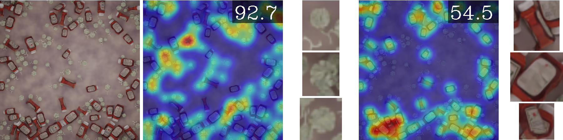
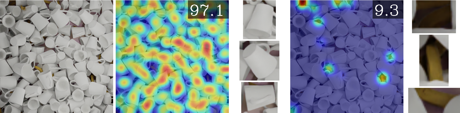
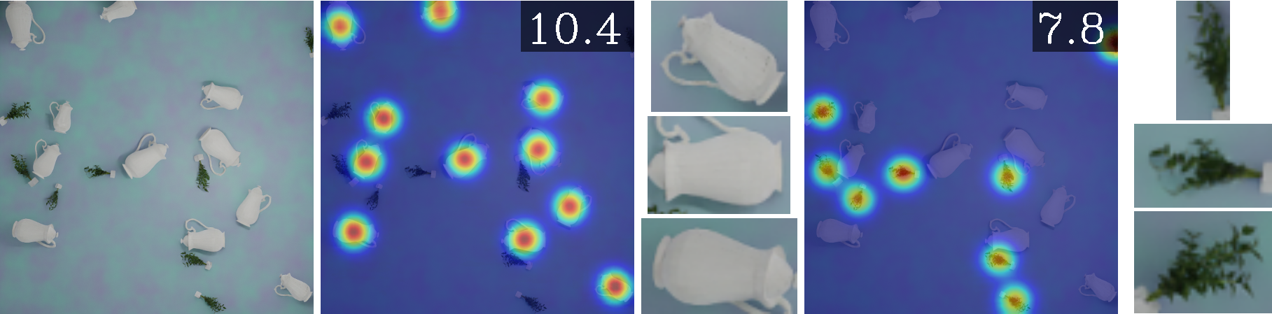
Figure 7: Example Finding. Using our density map predictions and a SAM [9] network, we can generate meaningful bounding boxes to aid a user in understanding what has been counted.

4.4 Implementation

We use ViT-Small [4] due to its lightweight nature and for comparison to methods that use the resnet-50 backbone, such as FamNet [16, 18]. ViT-S has a similar number of parameters (21M vs 23M), throughput (1237im/sec vs 1007im/sec), and supervised ImageNet performance (79.3% vs 79.8%) as ResNet-50 [20]. ABC123 is trainable in less than eight hours using two 1080Tis. It takes less than two hours to train just the head with a frozen backbone (ABC123❄).

Since vision transformers typically demand substantial training data, we initialised our transformer backbone with weights sourced from Caron et al. [2]. This self-supervised pre-training process endows the network with an understanding of meaningful image features prior to exposure to our dataset and without supervision. This approach reduces the risk of overfitting when the model is then trained on our dataset.

Our counting heads, comprised of 3 Conv-ReLU-Upsample blocks, increases the patch-wise resolution of the trained counting features from $k\times(28\times 28)$ to a pixel-wise density map prediction of $\hat{m}\times(224\times 224)$, where $k$ is the dimensionality of the transformer features and $\hat{m}$ is the number of predicted counts. For ABC123, $k=384$. We set $\hat{m}=5$ to ensure that the method has the capacity to generate a count per defined class in the dataset and at least one valid-but-unknown count. Our choice of ViT-S limits the resolution of our input image to (224$\times$224) as opposed to the $\geq$(384$\times$384) resolution used by contemporary methods with ResNet-50 or larger ViT backbones. For the example discovery stage, we use a frozen pretrained ViT-B SAM model [9].

5 Results

5.1 Benchmarking Methods

We evaluate our method against two trivial baseline methods, predicting the training-set mean or median count for all inference images. As there are no previous multi-class exemplar-free class-agnostic counting methods, we compare ABC123 to exemplar-based methods using separate exemplars from each of the classes present. We compare our method to FamNet [16], BMNet [18] and CounTR [11] on MCAC. Additionally, we compare to them and also RCC [6] and CounTR in its zero-shot configuration on MCAC-M1, the subset of MCAC with only a single type of object present per image.

To ensure a good comparison, we follow the suggested procedure laid out in Sec. 3.4, evaluating the exemplar-based methods using the bounding boxes of the three least occluded instances of a given class.

As in Xu et al. [24], we use Mean Absolute Error (MAE), Root Mean Squared Error (RMSE), Normalized Absolute Error (NAE), and Squared Relative Error (SRE) to evaluate the performance of each method.

$$MAE=\frac{1}{nm}\sum_{j=1}^{n}\sum_{i=1}^{m_{j}}|y_{i}-\hat{y_{i}}|$$

$$RMSE=\sqrt{\frac{1}{nm}\sum_{j=1}^{n}\sum_{i=1}^{m_{j}}(y_{i}-\hat{y_{i}})^{2}}$$

$$NAE=\frac{1}{nm}\sum_{j=1}^{n}\sum_{i=1}^{m_{j}}\frac{|y_{i}-\hat{y_{i}}|}{y_{i}}$$

$$SRE=\sqrt{\frac{1}{nm}\sum_{j=1}^{n}\sum_{i=1}^{m_{j}}\frac{(y_{i}-\hat{y_{i}})^{2}}{y_{i}}}$$

where $n$ is the number of test images, $m_{j}$ is the number of classes in image $j$, and $y_{i}$ and $\hat{y_{i}}$ are the ground truth and the predicted number of objects of class $i$ in image $j$ respectively.

5.2 MCAC

We achieve significantly better result than FamNet, BMNet, and CounTR on MCAC both quantitatively and qualitatively without needing exemplars; see Tab. 1 for results and Fig. 5 for comparative examples. As seen in Fig. 5, FamNet often fails to discriminate between objects of different kinds when they are visually similar or in high density applications. Both quantitatively and qualitatively, BMNet and CounTR outperform FamNet. However, in many cases, they appear to count the ‘most obvious’ objects in the image regardless of the provided exemplar images. Our method performs well on images with 4 classes even when they have high intra-class appearance variation, such as having different colours on different sides, and low inter-class variation; see Fig. 6. A downside to current exemplar-based class-agnostic counting methods is that while they have some multi-class capabilities, they all take a single exemplar at a time and produce only one count. This is slow and inefficient as compared to our method which generates all counts simultaneously.

As would be expected, the performance of all methods improves when evaluating on MCAC-M1, the images from MCAC with only a single class present; see Tab. 2. This is due to a lack of ambiguity as to the type to be counted. This was more significant when the methods were trained on MCAC-M1 instead of MCAC. In this training configuration, the methods generally learnt a broader definition of similarity as there was no chance they would accidentally combine classes or count instances from another class. RCC performs well on MCAC-M1, showing the strength of the simple count-wise loss in cases where there is little ambiguity as to what is to be counted. In contrast to other methods, ABC123 trained on MCAC-M1 has similar performance to when it is trained on the full MCAC dataset, demonstrating that it avoids the issues with other methods concerning intra-class variance and combining classes. Training ABC123 with only a single head ($\hat{m}=1$) and no matching stage has very similar performance to using its default ($\hat{m}=5$) configuration with a matching stage. This increases our belief that the matching head does not provide an unfair advantage to our method’s quantitative results.

5.3 Applicability to FSC-147/133

ABC123 trained on only MCAC, a synthetic dataset, produces accurate results when applied to FSC-133/147, a photographic dataset. However, it often finds valid-but-unknown counts. As seen in Fig. 8, the generated counts are correct for the type of object counted, but the type counted is often not aligned with the labels in the original dataset. Classes are often divided into sub-classes, and unlabelled classes are discovered.

There are two clear discrepancies between MCAC and FSC:

Cross domain image differences. As has been noted in many papers, applying a method solely trained on synthetic data to real data is likely to have negative results. Since images in the MCAC dataset are synthetic and simple, they do not reflect all of the variation found in FSC. For example, all images in MCAC are taken from above with no camera noise or harsh shadows. That being said, as is seen in Fig. 8, the generalised counting ability gained from training on MCAC clearly translates into the more varied and complex images in FSC.

Inter and Intra class differences. As discussed in Sec. 3, the labels in MCAC associate a count with objects of the same mesh and texture. FSC, however, is labelled by hand using high-level semantic understanding. This often leads to grouping of objects of significantly different geometries, colours, or textures under the same label. As seen in Fig. 8, when applying ABC123 trained on MCAC to images from FSC, we find that it often counts unlabelled classes, generates multiple identical counts because it enumerates different parts of the same objects, or subdivides classes by colour or geometry such as splitting ‘chairs’ into ‘red chairs’ and ‘grey chairs’. Novel class-discovery and duplicate part counts do not affect quantitative results on FSC as the matching stage removes them. However, sub-class counting causes erroneous numerical results. As our matching stage does not combine sub-class counts, only one of the sub-class counts is associated with the human labelled count. This generates a high numerical error and leads to poor quantitative results in the standard benchmark tests.

		Val Set				Test Set
Method	Shots	MAE	RMSE	NAE	SRE	MAE	RMSE	NAE	SRE
Mean	N/A	39.87	53.56	3.07	11.40	42.67	59.68	2.79	10.93
Median	N/A	36.25	58.15	1.51	6.70	39.81	65.36	1.38	6.73
Exemplar-based
FamNet+ [16]	3	24.76	41.12	1.12	6.86	26.40	45.52	1.04	6.87
BMNet+ [18]	3	15.83	27.07	0.71	4.97	17.29	29.83	0.75	6.08
CounTR [11]	3	15.07	26.26	0.63	4.79	16.12	29.28	0.67	5.71
Exemplar-free
ABC123 ❄	0	14.64	23.67	0.46	2.97	15.76	25.72	0.45	3.11
ABC123	0	8.96	15.93	0.29	2.02	9.52	17.64	0.28	2.23

Table 1: Comparison to SOTA methods on MCAC. We significantly outperform methods which use exemplar images and test-time adaptation without requiring them. ABC123❄ denotes our method trained with a frozen pre-trained backbone.

				Val Set				Test Set
Method	Multi-Class Training	Shots	$\hat{m}$	MAE	RMSE	NAE	SRE	MAE	RMSE	NAE	SRE
Mean	N/A	N/A	N/A	53.36	67.14	3.53	13.46	58.54	75.58	3.37	13.27
Median	N/A	N/A	N/A	45.98	76.64	1.08	6.68	51.35	86.61	1.03	7.00
Exemplar-based
FamNet+ [16]	✓	3	1	24.97	48.63	0.36	3.79	28.31	54.88	0.35	3.97
FamNet+ [16]	✗	3	1	12.54	24.69	0.37	4.71	13.97	26.19	0.25	2.12
BMNet+ [18]	✓	3	1	11.70	23.08	0.26	2.39	11.57	22.25	0.24	1.96
BMNet+ [18]	✗	3	1	6.82	12.84	0.25	2.95	8.05	14.57	0.19	1.43
CounTR [11]	✓	3	1	11.44	21.37	0.33	2.36	10.91	21.70	0.29	2.01
CounTR [11]	✓	0	1	13.57	25.53	0.30	2.48	13.09	25.72	0.29	2.41
CounTR [11]	✗	3	1	9.00	16.91	0.41	3.56	9.96	18.92	0.38	2.93
CounTR [11]	✗	0	1	9.16	17.13	0.42	3.56	10.10	19.10	0.40	3.02
Exemplar-free
CounTR†[11]	✗	0	1	11.46	21.24	0.35	2.78	12.54	23.84	0.31	2.38
RCC [6]	✗	0	1	7.78	15.40	0.24	2.71	8.81	16.92	0.19	1.73
ABC123 ❄	✗	0	5	10.78	18.83	0.28	1.97	13.23	24.57	0.29	2.39
ABC123 ❄	✗	0	1	11.38	19.73	0.40	3.51	14.31	25.40	0.37	2.79
ABC123 ❄	✓	0	5	10.98	18.85	0.30	1.93	13.13	23.93	0.29	2.18
ABC123	✗	0	5	5.82	11.74	0.15	1.22	7.54	15.30	0.21	1.87
ABC123	✗	0	1	5.85	12.91	0.24	3.37	7.53	15.69	0.22	2.19
ABC123	✓	0	5	6.08	12.62	0.16	1.22	6.82	14.70	0.16	1.51

Table 2: Comparison to SOTA methods on MCAC-M1. MCAC-M1 is the subset of MCAC with only one class present per image. Methods are either trained on the full multi-class dataset (✓) or MCAC-M1 (✗). ‘$\hat{m}$’ denotes the number of predictions the method generates per query and ‘Shots’ denotes the number of exemplar images per query at inference time. CounTR†is an exemplar-free adaption of CounTR as in Hobley and Prisacariu [6]. ABC123 outperforms other methods when trained in both single or multi-class settings.

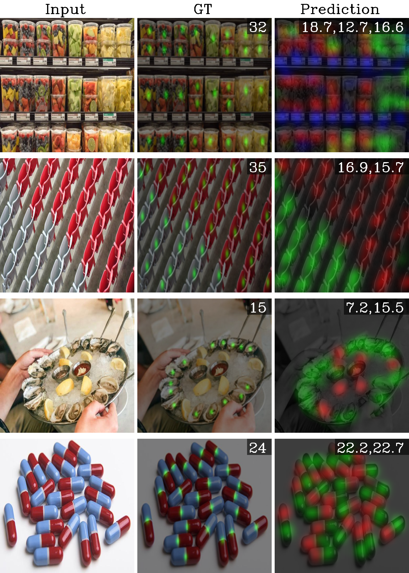
Figure 8: ABC123 method trained on MCAC applied to FSC-147. ABC123 generates accurate counts for the classes it locates. However, these classes are often not aligned with the human annotations. ABC123 often discovers unlabelled classes, divides labelled classes into sub classes by colour or shape, or counts the same object multiple times by subdividing each object into component parts. Centre: the ground truth (GT) density map is overlaid in green, Right: predicted density maps are overlaid in red, green, and blue, with the associated counts in the the top corner.

6 Ablations

In this section, we explain and validate various design decisions including our loss and matching stage scaling. We also show the effect that generating large numbers of predictions can have on quantitative benchmarks.

6.1 Validating Our Loss

Hobley and Prisacariu [6] showed that using image-wise count loss functions like the absolute count error could be beneficial over pixel-wise loss functions as they allow a network to learn its own idea of positional salience. We test our loss, the pixel-wise error $||d-\hat{d}||_{1}$, against both pixel-wise error squared $||d-\hat{d}||^{2}_{2}$, as in [16, 11, 24], and the image-wise count percentage error $\frac{|y-\hat{y}|}{y}$ [6], where $d$ and $\hat{d}$ are the ground truth and predicted density maps, and $y$ and $\hat{y}$ are the ground truth and predicted counts respectively.

Using an image-wise count loss creates poor results, with somewhat arbitrary density maps and incorrect counts. This is likely due to the matching stage. Whereas it usually operates on the density map to which the loss is directly applied, it now operates over an unconstrained latent feature. This, along with the added complexity of multi-class images, makes the problem significantly harder to understand from purely integer supervision. We also found that using a pixel-wise L₂ slightly degraded performance as compared to using the L₁ distance between the ground-truth and predicted density maps. Still, the predicted density maps were qualitatively meaningful. This discrepancy is likely due to the increased significance the higher-density edge-cases have on the training. See Tab. 3 for the quantitative comparison.

		Val Set				Test Set
Method	Loss	MAE	RMSE	NAE	SRE	MAE	RMSE	NAE	SRE
ABC123 ❄	Count-MAPE	19.88	38.20	0.48	3.62	25.32	49.18	0.52	4.28
ABC123 ❄	Pixel $L_{2}$	16.46	26.54	0.78	4.79	17.92	28.88	0.75	4.77
ABC123 ❄	Pixel $L_{1}$	14.64	23.67	0.46	2.97	15.76	25.72	0.45	3.11
ABC123	Count-MAPE	15.95	29.71	0.50	3.54	16.28	29.82	0.49	3.58
ABC123	Pixel $L_{2}$	10.76	19.31	0.49	3.84	11.91	21.42	0.51	4.21
ABC123	Pixel $L_{1}$	8.96	15.93	0.29	2.02	9.52	17.64	0.28	2.23

Table 3: Effect of different loss functions during training. Pixel-wise $L_{1}$ loss produces significantly better results than the pixel-wise $L_{2}$ loss and the count-wise MAPE.

6.2 Validating Our Matching Scaling

We found that normalising the density maps during training and testing was beneficial because it forced the network to generate the correct localisation as well as the correct magnitude. This normalisation also decreases the issue of the matcher cheating to find the correct count. Instead of selecting the correct count from a large set of predicted counts, the network must generate a density map with a correct localisation. Using the L₂ normalisation over the L_∞ has a slight performance increase for training the network and during evaluation. See Tab. 4 for qualitative comparison of the normalisations during the matching stage.

	Normalisation		Val Set				Test Set
Method	Train	Eval	MAE	RMSE	NAE	SRE	MAE	RMSE	NAE	SRE
ABC123 ❄	None	None	20.31	32.40	0.78	5.40	22.67	36.63	0.92	7.25
ABC123 ❄	None	L2	21.38	35.08	0.86	6.43	25.46	43.37	1.05	8.67
ABC123 ❄	None	L∞	20.13	32.15	0.81	5.86	22.76	36.78	0.95	7.64
ABC123 ❄	L2	None	41.20	66.04	0.87	6.22	45.04	73.41	0.87	6.51
ABC123 ❄	L2	L2	14.64	23.67	0.46	2.97	15.76	25.72	0.45	3.11
ABC123 ❄	L2	L∞	17.21	27.94	0.51	3.28	17.97	29.36	0.48	3.30
ABC123 ❄	L∞	None	22.40	35.80	0.73	4.89	23.93	38.59	0.80	5.86
ABC123 ❄	L∞	L2	17.92	28.98	0.67	5.12	20.40	33.39	0.77	6.24
ABC123 ❄	L∞	L∞	19.33	30.75	0.67	4.77	20.84	33.61	0.74	5.91
ABC123	None	None	15.46	28.49	0.60	5.12	16.15	29.82	0.69	6.50
ABC123	None	L2	14.83	27.25	0.68	6.15	17.04	31.88	0.84	8.06
ABC123	None	L∞	14.75	27.41	0.65	5.92	16.54	30.80	0.77	7.45
ABC123	L2	None	35.29	61.12	0.67	5.55	38.15	67.89	0.64	5.78
ABC123	L2	L2	8.96	15.93	0.29	2.02	9.52	17.64	0.28	2.23
ABC123	L2	L∞	9.95	18.16	0.32	2.22	9.89	18.55	0.29	2.20
ABC123	L∞	None	15.72	28.83	0.59	4.69	16.11	30.22	0.67	6.16
ABC123	L∞	L2	12.17	22.81	0.57	5.09	13.97	27.66	0.71	7.05
ABC123	L∞	L∞	12.46	23.00	0.56	4.90	13.96	27.12	0.66	6.37

Table 4: Effect of using normalised density maps for the matching stage. Normalisation improves the accuracy of ABC123. $L_{2}$ normalisation is more effective than $L_{\infty}$ during training and evaluation.

6.3 Validating Our Number of Predictions

As predicted, generating much larger numbers of predictions increases the quantitative performance of the network; see Tab. 5 for the complete results. This is because the network can generate more diverse counts and use the matching stage to select the best one. We believe, however, that this does not align with a more useful network in a deployment situation. This numerical gain derives purely from the matching stage, which is not present during deployment. In fact, during deployment, this would correspond to a much more difficult to interpret output as a user would have to figure out which of the many outputs was most relevant. We found that when high numbers of predictions were generate, fewer than half were used, i.e. the outputs of some heads were never picked. This is likely due to these heads not being matched frequently during training so the loss is rarely propagated back through them. There is also significant redundancy between the heads. The predictions of certain heads over the whole dataset were clearly similar and could be grouped. Of the 39 utilised heads, there were three groups of, respectively, 13, 6, and 4 heads that were very similar, lowering the effective number of utilised heads to 19.

$\hat{m}$	Val MAE	Channels Utilised	% Channel Utilisation
5	8.96	5	100%
10	8.39	10	100%
20	7.78	17	85%
50	7.26	34	68%
100	7.11	39	39%

Table 5: Effect of using more prediction heads. Increasing the number of pre-matching predictions improves the quantitative results of our method. However, as the number of heads increases, the percentage of heads that are frequently ($>0.4\%$) matched decreases.

7 Conclusion

In this work, we present ABC123, a multi-class exemplar-free class-agnostic counter, and show that it is superior to prior exemplar-based methods in a multi-class setting. ABC123 requires no human input at inference-time, works in complex settings with more than one kind of object present, and outputs easy to understand information in the form of examples of the counted objects. Due to this, it has good potential for deployment in various fields. We also propose MCAC, a multi-class class-agnostic counting dataset, and use it to train our method as well as to demonstrate that exemplar-based counting methods may not be as robust as previously assumed in multi-class settings.

A Class Splits

A.1 Training Classes

’1Shelves’, ’2Shelves’, ’3Shelves’, ’4Shelves’, ’5Shelves’, ’6Shelves’, ’7Shelves’, ’AAABattery’, ’AABattery’, ’AccentTable’, ’AirConditioner’, ’Airplane’, ’ArcadeMachine’, ’Armoire’, ’Ashtray’, ’Backpack’, ’Bag’, ’Ball’, ’BarCounter’, ’BarTable’, ’Barstool’, ’BaseballBat’, ’Basket’, ’Bathtub’, ’Battery’, ’BeanBag’, ’Bear’, ’Bed’, ’BeerBottle’, ’Bicycle’, ’Bidet’, ’Bird’, ’Blender’, ’Board’, ’Bottle’, ’Bookcase’, ’Booth’, ’Bowl’, ’Broom’, ’Bucket’, ’Bus’, ’Butterfly’, ’Cabinet’, ’Cabling’, ’Cage’, ’Camera’, ’CanOpener’, ’Canister’, ’CanopyBed’, ’Cap’, ’Carrot’, ’Cassette’, ’Cat’, ’CeilingFan’, ’CerealBox’, ’Chaise’, ’ChessBoard’, ’ChestOfDrawers’, ’ChildBed’, ’Chocolate’, ’Clock’, ’Closet’, ’Coaster’, ’CoatRack’, ’CoffeeMaker’, ’CoffeeTable’, ’Coin’, ’Compass’, ’Controller’, ’Cookie’, ’Couch’, ’Counter’, ’Courtyard’, ’Cow’, ’Cradle’, ’Credenza’, ’Cup’, ’CurioCabinet’, ’CuttingBoard’, ’DSLRCamera’, ’Dart’, ’DartBoard’, ’Desk’, ’Desktop’, ’Detergent’, ’DiningTable’, ’DiscCase’, ’Dishwasher’, ’Dog’, ’Donkey’, ’Door’, ’DoubleBed’, ’DraftingTable’, ’Dresser’, ’DresserWithMirror’, ’DrinkBottle’, ’DrumSet’, ’Dryer’, ’Easel’, ’Elephant’, ’EndTable’, ’Eraser’, ’Fan’, ’Fan CeilingFan’, ’Faucet’, ’FileCabinet’, ’Fireplace’, ’Fish’, ’FlagPole’, ’Flashlight’, ’Folder’, ’Futon’, ’GameTable’, ’Gamecube’, ’Giraffe’, ’Guitar’, ’GuitarStand’, ’Gun’, ’Hammer’, ’HandDryer’, ’Hanger’, ’Harp’, ’Hat’, ’Headboard’, ’Horse’, ’Ipad’, ’Ipod’, ’IroningBoard’, ’Kettle’, ’Key’, ’KingBed’, ’LDesk’, ’Ladder’, ’LampPost’, ’Laptop’, ’Lectern’, ’Letter’, ’LightBulb’, ’LightSwitch’, ’Lock’, ’LoftBed’, ’Loveseat’, ’Magnet’, ’Marker’, ’Mattress’, ’MediaChest’, ’MediaDiscs’, ’MediaPlayer’, ’MediaStorage’, ’Microscope’, ’Microwave’, ’MilkCarton’, ’Mirror’, ’Monitor’, ’Motorcycle’, ’Mouse’, ’MousePad’, ’Mug’, ’Nightstand’, ’NintendoDS’, ’Notepad’, ’Orange’, ’Ottoman’, ’OutdoorTable’, ’Oven’, ’OvenTop’, ’PS’, ’PS2’, ’PS3’, ’PSP’, ’Palette’, ’Pan’, ’Paper’, ’PaperBox’, ’PaperMoney’, ’Pedestal’, ’Pen’, ’Pencil’, ’Phone’, ’Phonebooth’, ’Piano’, ’PianoKeyboard’, ’PicnicTableSet’, ’Picture’, ’PillBottle’, ’Pizza’, ’Planet’, ’Plate’, ’Plotter’, ’PosterBed’, ’PotRack’, ’PowerSocket’, ’PowerStrip’, ’Purse’, ’QueenBed’, ’QueenBedWithNightstand’, ’Rabbit’, ’Rack’, ’Radio’, ’Recliner’, ’Refrigerator’, ’RiceCooker’, ’Ring’, ’Rock’, ’Room’, ’RoundTable’, ’Rug’, ’Ruler’, ’Sandwich’, ’Scale’, ’ScrewDriver’, ’Sectional’, ’Shampoo’, ’Ship’, ’Shirt’, ’Shoes’, ’ShoppingCart’, ’Shower’, ’Showerhead’, ’Sideboard’, ’SingleBed’, ’Sink’ ’Sleeper’, ’Snowman’, ’SoapBar’, ’SoapBottle’, ’SodaCan’, ’Speaker’, ’StandingClock’, ’StaplerWithStaples’, ’Statue’, ’Suitcase’, ’SupportFurniture’, ’Sword’, ’TV’, ’Table’, ’TableClock’, ’Tank’, ’Tape’, ’TapeDispenser’, ’TapeMeasure’, ’Teacup’, ’Telescope’, ’TelescopeWithTripod’, ’Tent’, ’Thermostat’, ’Thumbtack’, ’TissueBox’, ’Toaster’, ’ToasterOven’, ’Toilet’, ’Toothbrush’, ’TrashBin’, ’Truck’, ’Trumpet’, ’Trundle’, ’TvStand’, ’USBStick’, ’Umbrella’, ’Vanity’, ’Vase’, ’VideoGameConsole’, ’Stapler’, ’VideoGameController’, ’Violin’, ’WallClock’, ’WallLamp’, ’WallUnit’, ’Wallet’, ’Wardrobe’, ’Washer’, ’WasherDryerSet’, ’WebCam’, ’Whiteboard’, ’Wii’, ’Window’, ’WineBottle’, ’WineGlass’, ’WineRack’, ’Wood’, ’Xbox’, ’Xbox360’, ’Candle’, ’Car’, ’Blind’, ’Spoon’, ’Fork’, ’Knife’

A.2 Validation Classes

’Book’, ’Books’, ’Chair’, ’Stool’, ’Donut’, ’ChairWithOttoman’, ’Bench’, ’SideChair’, ’OfficeChair’, ’KneelingChair’, ’OfficeSideChair’, ’AccentChair’, ’CeilingLamp’, ’ComforterSet’, ’Computer’, ’Copier’, ’Curtain’, ’DecorativeAccessory’, ’DeskLamp’, ’FloorLamp’ ’Lamp’, ’PaperClip’, ’PersonStanding’, ’PictureFrame’, ’Pillow’, ’Printer’, ’Scissors’, ’TableDeskLamp’, ’TableLamp’, ’Teapot’, ’Throw’, ’WallArt’, ’Poster’, ’WallDecoration’, ’WallArtWithFigurine’, ’Painting’, ’SkateBoard’, ’ToiletPaper’

A.3 Testing Classes

’Animal’, ’Keyboard’, ’Calculator’, ’CellPhone’, ’ComputerMouse’, ’DrinkingUtensil’, ’FoodItem’, ’Headphones’, ’Helicopter’, ’Plant’, ’PottedPlant’, ’RubiksCube’, ’Telephone’, ’ToyFigure’, ’Watch’, ’Sheep’, ’Glasses’, ’Fruit’, ’FruitBowl’, ’Apple’

References

- Cao et al. [2018] Xinkun Cao, Zhipeng Wang, Yanyun Zhao, and Fei Su. Scale aggregation network for accurate and efficient crowd counting. In Proceedings of the European conference on computer vision (ECCV), pages 734–750, 2018.
- Caron et al. [2021] Mathilde Caron, Hugo Touvron, Ishan Misra, Hervé Jégou, Julien Mairal, Piotr Bojanowski, and Armand Joulin. Emerging properties in self-supervised vision transformers. In Proceedings of the IEEE/CVF International Conference on Computer Vision, pages 9650–9660, 2021.
- Crouse [2016] David F. Crouse. On implementing 2d rectangular assignment algorithms. IEEE Transactions on Aerospace and Electronic Systems, 52(4):1679–1696, 2016.
- Dosovitskiy et al. [2020] Alexey Dosovitskiy, Lucas Beyer, Alexander Kolesnikov, Dirk Weissenborn, Xiaohua Zhai, Thomas Unterthiner, Mostafa Dehghani, Matthias Minderer, Georg Heigold, Sylvain Gelly, et al. An image is worth 16x16 words: Transformers for image recognition at scale. In International Conference on Learning Representations, 2020.
- Go et al. [2021] Hyojun Go, Junyoung Byun, Byeongjun Park, Myung-Ae Choi, Seunghwa Yoo, and Changick Kim. Fine-grained multi-class object counting. In 2021 IEEE International Conference on Image Processing (ICIP), pages 509–513. IEEE, 2021.
- Hobley and Prisacariu [2023a] Michael Hobley and Victor Prisacariu. Learning to count anything: Reference-less class-agnostic counting with weak supervision. In Proceedings of the IEEE/CVF Conference on Computer Vision and Pattern Recognition, 2023a.
- Hobley and Prisacariu [2023b] Michael A Hobley and Victor A Prisacariu. Dms: Differentiable mean shift for dataset agnostic task specific clustering using side information. arXiv preprint arXiv:2305.18492, 2023b.
- Hoekendijk et al. [2021] Jeroen Hoekendijk, Benjamin Kellenberger, Geert Aarts, Sophie Brasseur, Suzanne SH Poiesz, and Devis Tuia. Counting using deep learning regression gives value to ecological surveys. Scientific reports, 11(1):1–12, 2021.
- Kirillov et al. [2023] Alexander Kirillov, Eric Mintun, Nikhila Ravi, Hanzi Mao, Chloe Rolland, Laura Gustafson, Tete Xiao, Spencer Whitehead, Alexander C. Berg, Wan-Yen Lo, Piotr Dollár, and Ross Girshick. Segment anything. arXiv:2304.02643, 2023.
- Lin et al. [2021] Hui Lin, Xiaopeng Hong, and Yabin Wang. Object counting: You only need to look at one. arXiv preprint arXiv:2112.05993, 2021.
- Liu et al. [2022] Chang Liu, Yujie Zhong, Andrew Zisserman, and Weidi Xie. Countr: Transformer-based generalised visual counting. arXiv preprint arXiv:2208.13721, 2022.
- Lu et al. [2018] Erika Lu, Weidi Xie, and Andrew Zisserman. Class-agnostic counting. In Asian Conference on Computer Vision, 2018.
- Ma et al. [2023] Zhiheng Ma, Xiaopeng Hong, and Qinnan Shangguan. Can sam count anything? an empirical study on sam counting. arXiv preprint arXiv:2304.10817, 2023.
- OpenAI [2023] OpenAI. Gpt-4 technical report, 2023.
- Ranjan and Hoai [2022] Viresh Ranjan and Minh Hoai. Exemplar free class agnostic counting. arXiv preprint arXiv:2205.14212, 2022.
- Ranjan et al. [2021] Viresh Ranjan, Udbhav Sharma, Thu Nguyen, and Minh Hoai. Learning to count everything. In Proceedings of the IEEE/CVF Conference on Computer Vision and Pattern Recognition, pages 3394–3403, 2021.
- Savva et al. [2015] Manolis Savva, Angel X. Chang, and Pat Hanrahan. Semantically-Enriched 3D Models for Common-sense Knowledge. CVPR 2015 Workshop on Functionality, Physics, Intentionality and Causality, 2015.
- Shi et al. [2022] Min Shi, Hao Lu, Chen Feng, Chengxin Liu, and Zhiguo Cao. Represent, compare, and learn: A similarity-aware framework for class-agnostic counting. In Proceedings of the IEEE/CVF Conference on Computer Vision and Pattern Recognition, pages 9529–9538, 2022.
- Sokhandan et al. [2020] Negin Sokhandan, Pegah Kamousi, Alejandro Posada, Eniola Alese, and Negar Rostamzadeh. A few-shot sequential approach for object counting. arXiv preprint arXiv:2007.01899, 2020.
- Touvron et al. [2021] Hugo Touvron, Matthieu Cord, Matthijs Douze, Francisco Massa, Alexandre Sablayrolles, and Hervé Jégou. Training data-efficient image transformers & distillation through attention. In International Conference on Machine Learning, pages 10347–10357. PMLR, 2021.
- Troisemaine et al. [2023] Colin Troisemaine, Vincent Lemaire, Stéphane Gosselin, Alexandre Reiffers-Masson, Joachim Flocon-Cholet, and Sandrine Vaton. Novel class discovery: an introduction and key concepts. arXiv preprint arXiv:2302.12028, 2023.
- Xie et al. [2016] Junyuan Xie, Ross Girshick, and Ali Farhadi. Unsupervised deep embedding for clustering analysis. In Proceedings of The 33rd International Conference on Machine Learning, pages 478–487, New York, New York, USA, 2016. PMLR.
- Xie et al. [2018] Weidi Xie, J Alison Noble, and Andrew Zisserman. Microscopy cell counting and detection with fully convolutional regression networks. Computer methods in biomechanics and biomedical engineering: Imaging & Visualization, 6(3):283–292, 2018.
- Xu et al. [2023] Jingyi Xu, Hieu Le, Vu Nguyen, Viresh Ranjan, and Dimitris Samaras. Zero-shot object counting. In Proceedings of the IEEE/CVF Conference on Computer Vision and Pattern Recognition, pages 15548–15557, 2023.
- Yang et al. [2021] Shuo-Diao Yang, Hung-Ting Su, Winston H Hsu, and Wen-Chin Chen. Class-agnostic few-shot object counting. In Proceedings of the IEEE/CVF Winter Conference on Applications of Computer Vision, pages 870–878, 2021.
- Yang et al. [2010] Yi Yang, Dong Xu, Feiping Nie, Shuicheng Yan, and Yueting Zhuang. Image clustering using local discriminant models and global integration. IEEE Transactions on Image Processing, 19(10):2761–2773, 2010.