Graph topological transformations in space-filling
cell aggregates

Abstract

Cell rearrangements are fundamental mechanisms driving large-scale deformations of living tissues. In three-dimensional (3D) space-filling cell aggregates, cells rearrange through local topological transitions of the network of cell-cell interfaces, which is most conveniently described by the vertex model. Since these transitions are not yet mathematically properly formulated, the 3D vertex model is generally difficult to implement. The few existing implementations rely on highly customized and complex software-engineering solutions, which cannot be transparently delineated and are thus mostly non-reproducible. To solve this outstanding problem, we propose a reformulation of the vertex model. Our approach, called Graph Vertex Model (GVM), is based on storing the topology of the cell network into a knowledge graph with a particular data structure that allows performing cell-rearrangement events by simple graph transformations. We find these transformations consinsting of transformation patterns corresponding to T1 transitions, thereby unifying topological transitions in 2D and 3D space-filling packings. This result suggests that the GVM’s graph data structure may be the most natural representation of cell aggregates and tissues. We use GVM to characterize solid-fluid transition in 3D cell aggregates, driven by active noise and find aggregates undergoing efficient ordering close to the transition point. In all, our work showcases knowledge graphs as particularly suitable data models for structured storage, analysis, and manipulation of tissue data, which potentially has paradigm-shifting implications for the fields of tissue biophysics and biology.

The mechanical interactions between individual cells and between the cells and their environment play a crucial role in determining the macroscopic properties and behaviors of animal tissues on a large scale [1, 2, 3, 4, 5, 6, 7]. During embryonic development, for example, forces generated within cellular cortices drive precise and highly orchestrated active deformations and collective cellular flows [8, 9, 10, 11, 12, 13]. The mechanical forces are transmitted across the tissue through cell-cell contacts, which form a complex spatial network with a dynamically changing topology [14, 15, 16, 17, 18, 19, 21, 20, 22, 23, 24, 25].

These cross-scale tissue mechanics have been addressed by computational models that represent cells as discrete entities with certain physical properties that phenomenologically describe the mechanics at smaller length scales [26, 27, 28, 29, 30, 31, 32, 33, 34, 35]. Arguably the most widely used and most detailed is the vertex model, which describes individual cells as polygons (2D) or polyhedra (3D) and parametrizes their shapes by vertex positions [36, 37, 38, 39]. Mechanical forces on the vertices are typically specified through a model potential energy, which effectively describes complex biomechanics of individual cells using only a small number of model parameters. Simulations of the vertex model include time integration of a system of dynamic equations for the vertices and topological transformations of the network of cell-cell interfaces accompanying cell rearrangements.

Conventional vertex models, which store the topology and geometry of the tissue in a tabular form within arrays, perform topological transformations by updating these arrays according to specified rules [40, 41, 42, 43]. Although programming the routines that perform these dynamic array updates is relatively manageable for planar polygonal cell packings and even for 3D surface packings involving polyhedral prism-like cells [44, 45, 46, 47, 48], developing computer codes for simulations of 3D bulk cell aggregates poses a significantly greater challenge. Indeed, since the pioneering work by Honda et al. [36], who first introduced a vertex model of 3D cell aggregates, there have only been a few recent works reporting successful attempts of coding a full 3D vertex model with dynamic cell rearrangements [49, 50, 51]. The main difficulty lies in the intricate architecture and extensive length of the codes necessary for implementing cell rearrangements with the conventional data model [40, 41, 42, 43], which raises questions about its suitability and challenges our basic understanding of rearrangements in space-filling packings.

To address these challenges, we introduce a reformulation of the vertex model called Graph Vertex Model (GVM). We discover a particular graph-data model, which allows formulating topological transformations of cell networks as simple graph transformations. The blueprint outlining the relationships among the components is specified through a metagraph which is designed in a manner that topological transformations are themselves represented by graphs. This design not only enhances their intuitive and visual understanding but also simplifies their implementation, making it accessible even to researchers with limited programming expertise. Furthermore, we show that within the GVM’s data representation, topological transformations in 3D space-filling packings become composites of T1 transitions and they exactly reduce to a single T1 transition when applied to a 2D system. This is a fundamental result that unifies rearrangements in 2D and 3D space-filling packings and suggests that GVM’s data model may be the most natural representation of these systems. As a proof of concept, we develop an open-source Python package neoVM, which implements GVM over a graph database, managed in Neo4j [52, 53]. We use our new approach to study solid-fluid transition in 3D cell aggregates. We characterize the transition and find aggregates undergoing most efficient ordering in the vicinity of the transition point.

Vertex model. A cell aggregate is represented as a three-dimensional packing of space-filling polyhedral cells (Fig. 1a). Cell shapes are parametrized by positions of vertices in the $(x,y,z)$ space:

$$\boldsymbol{r}_{i}=\left(x_{i},\>y_{i},\>z_{i}\right)\>.$$ (1)

Here $i=1,...,N_{v}$, where $N_{v}$ is the total number of vertices.

Pairs of vertices are connected by oriented edges, defined by the indices of the constituent vertices:

$$\underline{\boldsymbol{e}}_{j}=\left[+i^{(h)}_{j},\>-i^{(t)}_{j}\right]\>.$$ (2)

Here $i^{(h)}_{j}$ and $i^{(t)}_{j}$ denote indices of head and tail vertices of edge $j$, respectively (Fig. 1a), and $j=1,...,N_{e}$, with $N_{e}$ being the total number of edges. The signs of the vertex indices, $s_{j}^{(h/t)}=\pm 1$ denotes head and tail vertices of the edge. While at this point these signs seem redundant, since the order in which the indices appear in $\underline{\boldsymbol{e}}_{j}$ itself indicates the head/tail role of the corresponding vertices, they will become important later on.

Polygonal cell sides are defined by oriented lists of indices of their constituent edges as

$$\underline{\boldsymbol{p}}_{k}=\left[\sigma^{(\mu)}_{k}j^{(\mu)}_{k}\right]_{\mu=1,...,n_{k}^{(e)}}\>,$$ (3)

where $k=1,...,N_{p}$, with $N_{p}$ being the total number of polygons. The $n_{k}^{(e)}$ edges in the list $\underline{\boldsymbol{p}}_{k}$ are listed sequentially and $\sigma_{k}^{(\mu)}=\pm 1$ denotes the orientation of the $\mu$-th edge (with index $j^{(\mu)}_{k}$) within the polygon relative to a chosen positive direction (Fig. 1a).

Similarly, cells are defined by oriented lists of indices of the $n_{l}^{(p)}$ constituent polygons as

$$\underline{\boldsymbol{c}}_{l}=\left[\Sigma^{(\nu)}_{l}k^{(\nu)}_{l}\right]_{\nu=1,...,n_{l}^{(p)}}\>,$$ (4)

where $l=1,...,N_{c}$, with $N_{c}$ being the total number of cells within the aggregate. Polygon orientations $\Sigma^{(\nu)}_{l}=\pm 1$, where $-1$ and $+1$ correspond to the polygon’s normal vector pointing towards the cell center and away from the cell center, respectively (Fig. 1a). The direction of the polygon’s normal vector is defined by the right-hand-screw rule, where the fingers curl along the chosen polygon’s positive orientation of the bounding edges (Fig. 1a). In contrast to the case of polygons, $\underline{\boldsymbol{p}}_{k}$, polygon indices in $\underline{\boldsymbol{c}}_{l}$ need not be listed in any specific order.

A couple of exemplary structures of cell aggregates with $N_{c}=128$ cells is given in the online repository of neoVM [52].

The dynamics of cell-shape changes are described by simulating movements of the vertices, driven by mechanical forces. In a model that neglects inertial effects and only considers friction of vertices with a static ("ether-type") background, vertices follow first-order dynamics described by

$$\eta\frac{{\rm d}\boldsymbol{r}_{i}}{\rm dt}=-\nabla_{i}W+\boldsymbol{F}_{i}^{(a)}\>.$$ (5)

Here the $\eta$ is the friction coefficient, $W$ is the potential energy of the aggregate, and $\boldsymbol{F}_{i}^{(a)}$ is a system-specific active-force contribution. The potential energy is typically calculated from geometric properties of cells such as surface areas of cell-cell contacts $A$, cell volumes $V$, etc. These quantities are calculated from the vertex positions as sums over geometric elements, i.e., vertices, edges, polygons (Methods).

Topological transitions. In addition to changing their shapes, cells also change their relative organization within the tissue by exchanging their neighbors [36]. These reorganization events alter the topology of the network of cell-cell contacts, thereby also affecting the interaction between the vertices. In confluent cell aggregates, cells exchange their neighbors by (i) merging vertex pairs of vanishingly short edges and (ii) resolving these vertices into new edges [60, 58, 59]. The topology of the edge network after these transformations locally differs from the initial one. In particular, cells that were initially separated might become neighbors, whereas pairs of initially neigboring cells may separate.

To model cell rearrangements in 3D cell aggregates, the following elementary local topological trasformations need to be considered (Fig. 1b,c): (i) Edge-to-vertex (EV) transition merges vertices of a vanishingly short edge into a single 6-fold vertex, (ii) vertex-to-triangle (VT) transition resolves a 6-fold vertex into a new triangle, (iii) triangle-to-vertex (TV) transition merges all three vertices of a triangular polygon into a single 6-fold vertex, and (iv) vertex-to-edge (VE) transition resolves a 6-fold vertex into a new edge.

An EV followed by a VT completes an ET transition, which transforms a vanishing edge into a triangle, formed in the perpendicular direction to the shrinking edge (Fig. 1b,c). After an ET transition, initially separated cells become neighbors by sharing the new triangle. Similarly, a TV followed by a VE, completes a TE transition, which transforms a vanishing triangle into an edge, formed in the perpendicular direction to the shrinking triangle (Fig. 1b,c). After a TE transition, the neighboring cells initially sharing the triangle become separated. We note that in a special case of an epithelial monolayer, where cells only attach to their neighbors laterally but not apically and basally, EV transitions either on basal or apical edges give rise to scutoidal cells [61, 62].

Importantly, as illustrated in Fig. 1d, the 4 basic topological transformations are in fact composites of multiple edge-to-vertex and vertex-to-edge transitions, known in 2D polygonal networks, such that both ET as well as TE transition can be seen as combinations of triple T1 transitions of 4-polygon neighborhoods. In each T1 transition, a pair of initially neigboring polygons becomes separated, whereas polygons from the remaining (initially separated) polygon pair become neighbors. This suggests that, given an appropriate data representation, it should be possible to unify topological transformations in 2D and 3D space-filling packings. Consequently, implementing topological transformations in 3D polyhedral packings should be equally challenging than implementing T1 transitions 2D polygonal packings.

This observation directly contradicts the convoluted transformation algorithms from previous works on 3D cell aggregates and indicates the need for reformulating the vertex model’s core architecture. The main challenge underlying this task is to find a data model of cell aggregates, in which topological transitions are performed by trivial data transformations, representing most elementary operations, that are apparently common in 2D and 3D models (Fig. 1d).

Results

Conventional vertex models are implemented over tabular data models, which are based on storing cell configurations in arrays. The main issue with this type of approach is that vertices, edges, polygons, and cells are stored in separate arrays (${\boldsymbol{r}}_{i}$, $\underline{\boldsymbol{e}}_{j}$, $\underline{\boldsymbol{p}}_{k}$, and $\underline{\boldsymbol{c}}_{l}$, respectively), which do not directly encode any interconnections or relationships among their respective elements. In particular, elements that might be spatially and topologically related are generally not stored together in the database and accessing any high-level topology data (e.g., finding cells that share a common vertex) requires inefficient searches over all the elements of the cell network.

To avoid these inefficient searches, the conventional vertex models store data in a highly redundant form, where higher-level information about the topology of the cell network are stored in addition to $\underline{\boldsymbol{e}}_{j}$, $\underline{\boldsymbol{p}}_{k}$, and $\underline{\boldsymbol{c}}_{l}$ (even though these higher-level information may be calculable from $\underline{\boldsymbol{e}}_{j}$, $\underline{\boldsymbol{p}}_{k}$, and $\underline{\boldsymbol{c}}_{l}$). For instance, to efficiently search for cells that share a certain vertex, lists of cells sharing a common vertex need to be stored for all vertices. Indeed, retreiving this information from $\underline{\boldsymbol{e}}_{j}$, $\underline{\boldsymbol{p}}_{k}$, and $\underline{\boldsymbol{c}}_{l}$ on the fly would require highly inefficient looping over all the cells. Due to this data redundancy, algorithms that manipulate the data arrays upon topological transformations in a self-consistent manner are difficult to program.

Knowledge graph. To overcome these issues, we propose a new approach, based on storing the topology of the cell network into a knowledge graph, which uses a graph- rather than a tabular data model. By construction, the elements that are topologically related are also connected in the knowledge graph and therefore, any high-level information about the topology of the cell network is readily retrievable by querying over the relevant part of the database with no need of storing any redundant data.

Knowledge graph is a graph data structure, which represents a network of real-world entities and relationships between them [63]. These data are stored in a graph database where entities and relationships are represented by nodes and links, respectively, and can, additionally, carry multiple properties. For example, a movie database can be stored as a knowledge graph, in which the data about actors and directors for a given movie are represented by nodes labeled Person and Movie and relationships labeled ACTED_IN and DIRECTED. In such a knowledge graph, the information that Cillian Murphy acted in the movie Oppenheimer, directed by Christopher Nolan, can be stored as (p1:Person {name: "Cillian Murphy"})-[:ACTED_IN]->(m:Movie {title: "Oppenheimer"})<-[:DIRECTED]-(p2:Person {name: "Christopher Nolan"}); here nodes labeled Person and Movie carry the name and the title properties, respectively.

The notation used here and in the following sections follows the syntax of the Cypher graph query language [64]. It is important to note that GVM relies on general principles of discrete mathematics and does not depend neither on the choice of the query language nor on the choice of the database-management framework.

Metagraph. Real-world entities in GVM are vertices, edges, polygons, and cells and they are stored in a knowledge graph in a hierarchical manner as nodes labeled Vertex, Edge, Polygon, and Cell, respectively. The topology of the cell network is encoded through relationships labeled IS_PART_OF. These relationships are directed and relate source-target node pairs, where the entity represented by the source node is always hierarchically one level below the entity represented by the target node.

For instance, if a specific polygon $p$ contains a specific edge $e$, the nodes representing these two entities, i.e., (p) and (e), are connected as (e)-[:IS_PART_OF]->(p). Connecting equally labeled nodes (e.g., a pair of edges) is not allowed and neither is connecting nodes carrying labels that do not follow one another hierarchically (e.g., a vertex-polygon pair). For example, say that one of the polygon $p$’s vertices is vertex $v$. Rather than encoding the information that $v$ is part of $p$ directly by a (v)-[:IS_PART_OF]->(p) connection, this information is retrieved hierarchically from the connectivity of $v$ and $p$ through edges. In particular, if $v$ is part of $p$, it is also necessarily shared by two edges that are both also part of $p$ (say $e_{1}$ and $e_{2}$): (v)-[:IS_PART_OF]->(e1)-[:IS_PART_OF]->(p) and (v)-[:IS_PART_OF]->(e2)-[:IS_PART_OF]->(p). An extra connection (v)-[:IS_PART_OF]->(p) would be redundant and is therefore forbidden in GVM, since these two subgraphs already imply that $v$ is one of polygon $p$’s vertices.

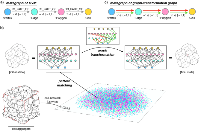
Figure 2: Graph Vertex Model. a The hierarchical structure of GVM vertex$\to$edge$\to$polygon$\to$cell is defined by a metagraph. Relationships between these nodes are labeled IS_PART_OF and carry a sign property denoted by $s$, $\sigma$, and $\Sigma$ for vertex$\to$edge, edge$\to$polygon, and polygon$\to$cell relationships, respectively. b Pattern matching a subgraph representing a particular local cell state, subject to a rearrangement event. This graph is then transformed by a graph transformation. c Metagraph of graph-transformation graph connects Vertex, Edge, Polygon, and Cell nodes with green and red relationships, indicating creation and deletion of IS_PART_OF relationships in the GVM’s knowledge graph.

The above rules for the construction of the GVM’s knowledge graph can be conveniently represented by a graph, called metagraph. Much like metalanguage is a language that describes another language, metagraph is a graph that describes another graph and can be viewed as a blueprint for generating actual (valid) manifestations of that graph. From the above definitions, it is obvious that the metagraph of GVM is (:Vertex)-[:IS_PART_OF]->(:Edge)-[:IS_PART_OF]->(:Polygon)-[:IS_PART_OF]->(:Cell) (Fig. 2a).

Additionally, both nodes and relationships carry properties that encode additional knowledge about nodes and relationships. While nodes carry a property, id, which represents the identification numbers $i$, $j$, $k$, and $l$ of vertices, edges, polygons, and cells, respectively, the relationships are prescribed a property sign, whose value is either $-1$ or $+1$. This is a contextual property, that puts the relationship’s source node into the context of the target node. In particular, in the subgraphs of type (v:Vertex)-[r:IS_PART_OF]->(e:Edge), the value of r.sign denotes whether vertex $v$ is a head vertex (r.sign=+1) or a tail vertex (r.sign=-1) of edge $e$ [i.e., parameter $s$ in Eq. (2)]. In the subgraphs of types (e:Edge)-[r:IS_PART_OF]->(p:Polygon) and (p:Polygon)-[r:IS_PART_OF]->(c:Cell) the same property specifies the orientation of edge $e$ in the context of polygon $p$ and polygon $p$ in the context of cell $c$, respectively [i.e., parameters $\sigma$ and $\Sigma$ in Eqs. (3) and (4), respectively].

Pattern matching. Transforming the graph database of GVM upon cell rearrangements requires only two steps: (i) Data retrieval, accomplished through pattern matching and (ii) Graph transformation. In step (i), a suitable (meta)graph pattern is utilized to query the database and identify the nodes relevant to the transformation at hand. After the graph is traversed, instances of the specified graph pattern are returned. If needed, these instances can be further filtered, using various conditional statements. For example, in an EV transition on edge $i$, the nodes representing polygons $p_{1}$, $p_{2}$, and $p_{3}$ (Fig. 1c) are found by a short query, shown in Eq. (18).

The goal of step (i) is to retrieve from the whole graph of GVM a small subgraph comprising solely of the nodes representing the objects (vertices, edges, polygons, and cells) that take part in the specific topological transformation being performed (Fig. 2b). Given the unambiguous definition of the graph data structure by the GVM’s metagraph (Fig. 2a), the routines that perform this step are easily reproducible. We implement these routines in Cypher and find that each topological transition requires $\sim 10$ distinct short queries, similar to the query shown in Eq. (18) [52] to retrieve the relevant data.

Graph transformations. In step (ii), the subgraph matched during the pattern-matching step undergoes a transformation based on the rules of the specific cell-rearrangement event being performed.

Like the matched subgraph that is being transformed, the graph transformation itself is represented by a graph. This graph contains exactly the same nodes as the matched GVM subgraph, however with much fewer relationships. In particular, the relationships in the transformation graph are of two types: (i) Green and (ii) red, indicating creations and deletions of :IS_PART_OF relationships in the actual GVM subgraph, respectively (Fig. 2c).

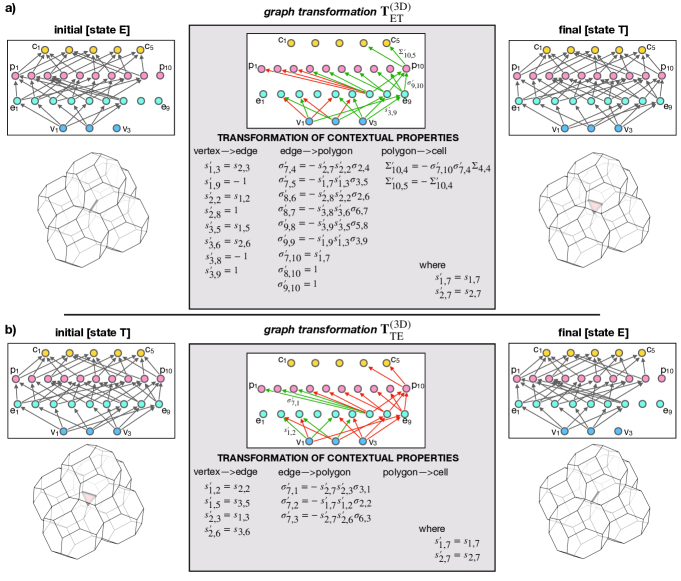
Figure 3: Graph transformations in a 3D vertex model of polyhedral packings. a Graph transformation of an ET transition. b Graph transformation of an TE transition. In both panels, graphs in the left and the right column correspond to the initial and the final cell configuration, respectively. Gray arrows represent relationships labeled IS_PART_OF. The graphs in the middle column show graph transformations, which include green and red relationships, indicating relationship creations and deletions, respectively. Additionally, the graph transformation specifies property values of the newly created relationships. In each graph, the node indices increase from left to right in unit steps.

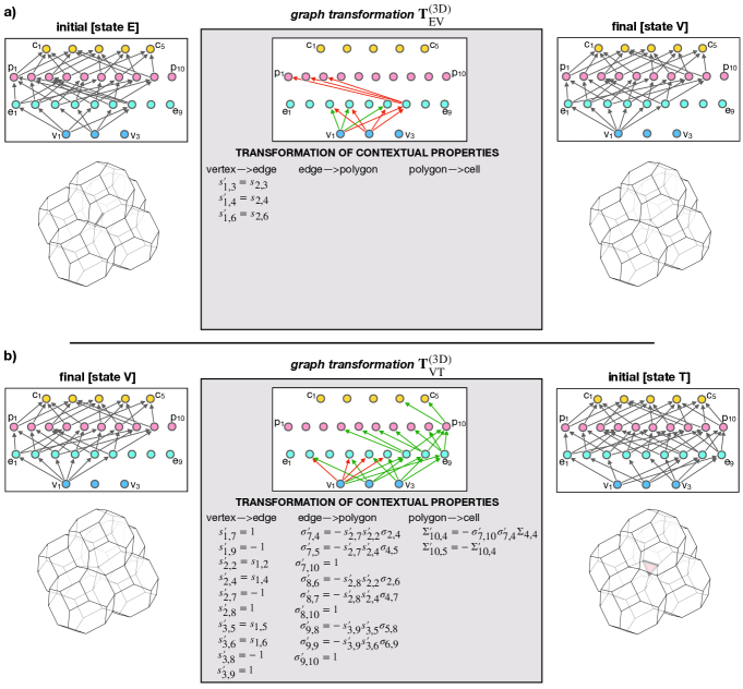
Figure S1: Graph transformations of EV and VT transitions . (panels a and b, respectively). Graphs in the left and the right column correspond to the initial and the final cell configuration, respectively. Gray arrows represent relationships labeled IS_PART_OF. The graphs in the middle column show graph transformations, which include green and red relationships, indicating relationship creations and deletions, respectively. Additionally, the graph transformation specifies property values of the newly created relationships. In each graph, the node indices increase from left to right in unit steps.

For instance, a green relationship between nodes representing vertex $v_{1}$ and edge $e_{3}$ indicates creation of a new relationship between previously matched nodes (v1) and (e3) [Eq. (19)]. Similarly, a red relationship between edge $e_{5}$ and polygon $p_{4}$, for example, indicates deletion of the relationship between previously matched nodes (e5) and (p4) [Eq. (20)]. Figure 3 shows graph transformations for ET and TE transformations as well as the matched subgraphs representing initial and final cell configurations. Graph transformations for EV, VT, TV, and VE transformations are given in Figs. S1 and S2. For clarity, the graphs representing all three states (E, T, and V) are additionally specified in a more explicit (non-pictorial) form in Methods.

Compared to the convoluted codes that perform topological transformations in the conventional vertex model, the task of programming the routines that perform topological transformations in GVM is much less challenging. Indeed, our implementation of graph-transformation routines in Cypher comprises of successive calls of $\sim 5$ distinct short queries, similar to examples shown in Eqs. (19) and (20).

Transformation of contextual properties. Values of contextual properties $s$, $\sigma$, and $\Sigma$ to be assigned to the newly created relationships are specified in the transformation graph through the relationship property of green relationships ($s^{\prime}$, $\sigma^{\prime}$, and $\Sigma^{\prime}$ for vertex$\to$edge, edge$\to$polygon, and polygon$\to$cell connections, respectively). Unlike the green relationships, the red relationships do not carry any additional properties (Fig. 2c).

Contextual properties of the newly created relationships are easily calculable and are exactly specified in Fig. 3. In particular, for a new vertex$\to$edge relationship between nodes representing vertex $v_{i}$ and edge $e_{j}$, $s^{\prime}_{i,j}$ is calculated as

$$s_{i,j}^{\prime}=s_{k,j}\>,$$ (6)

where $k$ denotes vertex $v_{k}$, which was part of edge $e_{j}$ prior to the transformation (i.e., $s_{k,j}$ denotes contextual property of the relationship between nodes representing vertex $v_{k}$ and edge $e_{j}$ prior to the transformation).

For a new edge$\to$polygon relationship between nodes representing edge $e_{i}$ and polygon $p_{j}$, $\sigma^{\prime}_{i,j}$ is calculated as

$$\sigma_{i,j}^{\prime}=-s_{k,i}^{\prime}s_{k,l}^{\prime}\sigma_{l,j}\>.$$ (7)

Here, vertex $v_{k}$ is a vertex shared by edges $e_{i}$ and $e_{l}$, which are both part of polygon $p_{j}$. Additionally, among the two vertices of edge $e_{i}$, vertex $v_{k}$ is the one that was not part part of edge $e_{l}$ prior to the transformation (i.e., Eq. (7) contains $s_{k,l}^{\prime}$ and not $s_{k,l}$). An analogous equation to Eq. (7) also holds for assigning $\Sigma^{\prime}_{ij}$ to a newly created polygon$\to$cell relationship (i.e., $\Sigma^{\prime}_{10,4}$ in Fig. 3a).

Note that values of contextual properties of certain newly created relationships need not be calculated, but can be either chosen arbitrarily or their values are automatically imposed (Fig. 3).

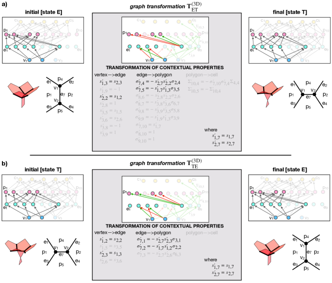
Figure 4: Graph transformations of ET and TE transitions reduce to a T1 transition. a ET transformation when applied to a four-polygon neighborhood. b TE transformation when applied to a four-polygon neighborhood. In both panels, those nodes and relationships from the original ET and TE transformations (Fig. 3) that are not matched are displayed transparent. The remaining opaque, i.e., matched, nodes and relationships exactly describe a T1 transformation. This shows that ET and TE transformations contain common transformation patterns, representing composites of T1 transitions, thereby unifying transformations in 2D and 3D space-filling packings. Graph transformation of a T1 transition contains 2 vertex$\to$edge relationship deletions, 2 vertex$\to$edge relationship creations, 2 edge$\to$polygon relationship deletions, and 2 edge$\to$polygon relationship creations (Fig. S3).

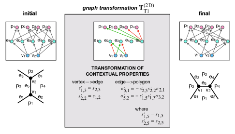
Figure S3: Graph transformation for a T1 transition. Graphs in the left and the right column correspond to the initial and the final cell configuration, respectively. Gray arrows represent relationships labeled IS_PART_OF. The graph in the middle column shows the graph transformation, which includes green and red relationships, indicating relationship creations and deletions, respectively. Additionally, the graph transformation specifies property values of the newly created relationships. In each graph, the node indices increase from left to right in unit steps.

Generalization of topological transformations. In agreement with our observation that topological transformations in 3D polyhedral packings are composites of more elementary topological (T1) transformations in 2D polygonal networks (Fig. 1d), we find that graph transformations ${\bf T}_{\rm ET}^{\rm(3D)}$ and ${\bf T}_{\rm TE}^{\rm(3D)}$ both contain transformation patterns corresponding to T1 transitions (Fig. 4 and Fig. S3). This result generalizes ET and TE topological transformations to "multidimensional" T1 transitions.

Moreover, both ${\bf T}_{\rm ET}^{\rm(3D)}$ and ${\bf T}_{\rm TE}^{\rm(3D)}$ simplify to a single T1 transition when applied to an edge in a polygonal network (Fig. 4). Even though ${\bf T}_{\rm ET}^{\rm(3D)}$ and ${\bf T}_{\rm TE}^{\rm(3D)}$ both assume the input subgraph of a form with 5 cell nodes, 10 polygon nodes, 9 edge nodes, and 3 vertex nodes, exactly the same transformations can be applied to a subragph representing a 4-polygon neighborhood in a 2D polygonal packing, undergoing a T1 transition. In this case, the pattern-matching step only matches 2 vertices, 5 edges, and 4 polygons and only a subset of graph-transformation operations (4 relationship creations, 4 relationship deletions, and 6 property assignings) are perfrormed (Fig. 4 and Fig. S3). This result unifies topological transformations in 2D and 3D systems, suggesting that GVM’s data structure may be the most natural representation of space-filling polyhedral packings.

Active tissue fluidization. As a proof of concept, we develop a custom Python package called neoVM, which manages the GVM’s knowledge graph and its transformations in a graph database management framework Neo4j (Methods).

We use neoVM, to study fluidization of cell aggregates by active tension fluctuations. In particular, we consider an aggregate of $N_{c}=128$ cells, enclosed within a simulation box with periodic boundary conditions. The vertex dynamics are described by Eq. (5), assuming the potential energy given by Eq. (10). In addition to the conservative and friction forces, we also include active force dipoles acting along cell edges to induce active cell rearrangements. The total active force on vertex $i$ is a sum of forces acting along edges (i.e., tricellular junctions) sharing that same vertex:

$$\boldsymbol{F}_{i}^{(a)}=-\sum_{lmn}\gamma_{lmn}(t)\nabla_{i}L_{lmn}\>.$$ (8)

Here the indices $lmn$ denote a tricellular junction (i.e., edge), shared by cells $l$, $m$, and $n$; $L_{lmn}$ is the edge length.

The magnitudes of active force dipoles are dynamic quantities that fluctuate with time. In particular $\gamma_{lmn}(t)$ obeys Ornstein-Uhlenbeck dynamics described by

$$\dot{\gamma}_{lmn}(t)=-\frac{1}{\tau_{m}}\left(\gamma_{lmn}(t)-\gamma_{0}\right)+\xi_{lmn}(t)\>,$$ (9)

where $\tau_{m}$ is the relaxation time scale associated with turnover dynamics of molecular motor Myosin, $\gamma_{0}$ is a baseline tension, whereas $\xi_{lmn}(t)$ is Gaussian white noise with properties $\langle\xi_{lmn}(t)\rangle=0$ and $\langle\xi_{lmn}(t)\xi_{opr}(t^{\prime})\rangle=\left(2\sigma^{2}/\tau_{m}\right)\delta_{lo}\delta_{mp}\delta_{nr}\delta(t-t^{\prime})$; $\sigma^{2}$ is the long-time variance of the tension fluctuations.

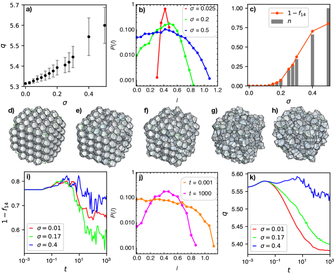
Figure 5: Solid-fluid transition in 3D cell aggregates. a Shape parameter $q$ for “thermalized” aggregates versus active noise $\sigma$. b Distribution of edge lengths in thermalized aggregates for $\sigma=0.025,\>0.2,\>{\rm and\hskip 2.84544pt}\>0.5$ (red, green, and blue curves, respectively). c Order parameter $1-f_{14}$ and normalized number of cell-rearrangement events $n=(N_{\rm ET}+N_{\rm TE})/N_{\rm max}$ versus active noise $\sigma$. d-h Thermalized aggreages at $\sigma=0,0.2,0.3,0.4,{\rm and\hskip 2.84544pt}0.5$. i Order parameter $1-f_{14}$ versus time for $\sigma=0.01,\>0.17\>{\rm and}\>0.4$ (red, green, and blue curves, respectively) during aggregate ordering. j The initial ($t=0.001$; orange curve) and final ($t=1000$; magenta curve) distributions of edge lengths at $\sigma=0.17$. k Shape parameter $q$ versus time for $\sigma=0.01,\>0.17\>{\rm and}\>0.4$ (red, green, and blue curves, respectively) during aggregate ordering.

We simulate the above active dynamics at different magnitudes of active noise $\sigma$, starting with a Kelvin structure–a crystalline cell arrangement made up of truncated octahedra with 14 facets (8 regular hexagons and 6 squares). The active noise distorts the geometry of the aggregates, which are no longer perfect crystals. In particular, for $\sigma>0$ the average cell shape, quantified by the shape factor $q=\langle S_{l}/V_{l}^{2/3}\rangle_{l\in{\rm cells}}$ ($S_{l}$ and $V_{l}$ are cell surface area and volume, respectively) deviates from the Kelvin’s truncated octahedron (Fig. 5a). The distorted geometry is also seen in the width of the distribution of edge lengths, which increases with an increasing $\sigma$–to a point where vanishingly short edges appear (Fig. 5b). These edges undergo ET and TE topological transformations, which in turn triggers cell rearrangements–a signature of a transition from a solid- to a fluid-like behavior. This transition is seen in the dependence of an order parameter $1-f_{14}$, describing the fraction of non-14-sided polyhedra ($f_{14}=N_{14}/N_{c}$), on the control parameter $\sigma$ (Fig. 5c). From these results, we obtain an estimate for the transition point $\sigma^{*}\approx 0.17$. Figs. 5d-h show cell configurations at $\sigma=0,0.2,0.3,0.4,{\rm and\hskip 2.84544pt}0.5$.

Next, we are interested in whether the active noise can drive the opposite effect, i.e., ordering. To study this, we start with a disordered cell packing, prepared in advance by packing spheres in the simulation box, using random sequential addition and then constructing Voronoi partitions around sphere centers. This procedure yields a sample with the initial fraction of 14-sided polyhedra $f_{14}=0.234$. Again, we simulate the active dynamics at different magnitudes of the active noise $\sigma$. We find that high-$\sigma$ values keep the aggregate disordered due to frequent cell-neighbor exchanges. In contrast, a sufficiently small level of active noise drives active tissue ordering, which is seen in decreasing $1-f_{14}$ and narrowing of the edge-length distribution over time (Fig. 5i and Fig. 5j, respectively). At moderate $\sigma\approx\sigma^{*}$ values, the ordering is more efficient compared to small $\sigma$ values, where the active-noise level is not sufficient to allow overcoming local energy barriers for cell rearrangements. Despite a higher degree of disorder, the low-$\sigma$ states consist of cells whose shapes are closer to the Kelvin’s regular truncated octahedron compared to cells from the $\sigma\approx\sigma^{*}$ case, where cell shapes are perturbed due to active noise (Fig. 5k).

The rate of topological-transition events in the simulations of active cell aggregates reaches as high as $\sim 200/{\rm time\>unit}$, which in total amounts to $\sim 10^{5}$ events per simulation (Fig. 5c); note that many of these events are reversible transitions that occur multiple times while the manipulated vertices are still located very close to one another and have not yet properly resolved in geometric sense. Despite this large number of reconnections, the aggregate keeps its integrity, demonstrating that topological transformations in space-filling 3D packings can indeed be implemented as graph transformations defined in Figs. 3 and 4. Importantly, due to GVM’s unambiguous data structure, these transformations are relatively straight-forward to implement and are therefore readily reproducible, which is clearly demonstrated by the implementation of GVM within our neoVM package [52].

Discussion. We reformulated the vertex model of cell aggregates. The new formulation, called Graph Vertex Model (GVM), is based on storing the topology of the cell network into a knowledge graph. We discovered a particular graph data model, uniquely defined by a metagraph, which allows formulating topological transformations of the cell network as simple and mathematically properly defined graph transformations (Fig. 2). These transformations are themselves represented by graphs and consist of only the most elementary graph operations, i.e., node and relationship deletions and creations.

We designed graph transformations for all topological transitions, required to describe cell rearrangements–including edge-to-triangle (ET) and triangle-to-edge (TE) transformations (Fig. 3). We showed that ET and TE transformations are inherently of the same type since they are both merely composites of transformation patterns corresponding to T1 transitions (Fig. 4). Imporantly, when applied to a 2D system, both ET and TE transformations reduce to a single T1 transition, thereby unifying topological transformations in 2D and 3D space-filling packings (Fig. 4). These fundamental insights surfaced due to the particular graph data structure of GVM, which seems to be the most natural representation of the topology of space-filling packings. We used GVM to study active cell aggregates, whose cell junctions are subject to fluctuating active tensions (Fig. 5). In particular, we characterized the solid-to-fluid transition and found disordered aggregates undergoing ordering, which is most efficient for active noise close to the transition point.

Our work represents a pioneering effort in introducing graph databases into the fields of tissue mechanics and biology. Even though the basic GVM’s data model presented here only encodes information on the topology of cell networks, GVM already represents an important technological and conceptual step forward in computational models of tissue mechanics. This advancement lays the foundation for the creation of knowledge graphs capable of structurally storing live-imaging data, such as that obtained from developing embryos. This involves integrating data on geometry, topology, mechanics, and biochemistry. With this aim, our ongoing work uses GVM as a starting point to develop a comprehensive knowledge-graph database of the early fly development [65]. By making this database interactive and accessible online will allow collaborative research with the aim to progressively expand our collective knowledge base about the mechanics of the embryonic development. Additionally, its graph data structure may even be readily complemented with graph-compatible methods of artificial intelligence (e.g., Graph Neural Networks).

In the context of computational modelling, a considerable effort will also have to be devoted to developing technologies that will improve computational efficiency of the vertex-model simulations over a graph database. While our current implementation of GVM, neoVM [52], primarily serves as a proof of concept, it falls short on the efficiency. The reason for this is mostly twofold: (i) The time integration of the dynamical system is performed in Python, which is generally slower than some low-level programming languages, and (ii) Performing operations on the graph database managed by Neo4j necessitates reading from and writing to the local hard drive, where the database is stored. The latter could be improved by relying on the memory storage instead.

Methods

Calculation of forces. We neglect the inertial effects so that the friction force $\boldsymbol{F}_{i}^{(f)}$ needs to counterbalance the sum of conservative and active forces, $\boldsymbol{F}_{i}^{(c)}$ and $\boldsymbol{F}_{i}^{(a)}$, respectively. This implies $\boldsymbol{F}_{i}^{(f)}+\boldsymbol{F}_{i}^{(c)}+\boldsymbol{F}_{i}^{(a)}=0$, where the conservative force $\boldsymbol{F}_{i}^{(c)}=-\nabla_{i}W$, with $W$ being the potential energy of the system, whereas $\boldsymbol{F}_{i}^{(f)}=-\eta\dot{\boldsymbol{r}}_{i}$. Here, only friction with a static (“ether-type”) background is considered, $\eta$ being the associated friction coefficient. The active force $\boldsymbol{F}_{i}^{(a)}$ can describe different system-specific active mechanisms, e.g., active contractions of the cell membrane due to the activity of the underlying cell cortex or traction forces [19, 20, 54, 32]. This model yields a system of first-order dynamic equations for vertex positions given by Eq. (5).

We consider a model, in which cell-cell interfaces are prescribed by effective surface tensions $\Gamma_{lm}$, which include contributions of the cell cortical tension and cell-cell adhesion [55, 56, 57]; the notation $lm$ denotes index of a polygon shared by cells $l$ and $m$. In this model, the total potential energy of the cell aggregate reads

$$W=\sum_{\left<lm\right>}\Gamma_{lm}A_{lm}+\kappa_{V}\sum_{l}\left(V_{l}-V_{0}\right)^{2}\>,$$ (10)

where the first sum goes over all pairs of neighboring cells $l$ and $m$ and the second sum goes over all the cells, $\kappa_{V}$ and $V_{0}$ being the cell-incompressibility constant and the preferred cell volume, respectively.

By definition, the conservative force acting on vertex $i$ is calculated as

$$\boldsymbol{F}_{i}^{(c)}=-\sum_{\left<lm\right>}\Gamma_{lm}\nabla_{i}A_{lm}-2\kappa_{V}\sum_{l}(V_{l}-V_{0})\nabla_{i}V_{l}\>,$$ (11)

which further requires calculating gradients of interfacial surface areas and cell volumes as described below.

Surface area of polygonal side $k$ is calculated as a sum of surface areas of triangular surface elements, $\big{\lVert}\boldsymbol{a}_{lm,\mu}\big{\rVert}$, defined by pairs of consecutive polygon vertices $\boldsymbol{r}_{\mu}$ and $\boldsymbol{r}_{\mu+1}$, and the polygon’s center of mass

$$\boldsymbol{c}_{lm}=\frac{1}{n_{lm}}\sum_{\mu\in\langle lm\rangle}\boldsymbol{r}_{\mu}\>.$$ (12)

Like in the previous section, Greek indices here do not denote the real vertex identification numbers, but their sequential indices within individual polygons. The surface area of polygon $lm$ reads

$$A_{lm}=\sum_{\mu\in\langle lm\rangle}\frac{1}{2}\big{\lVert}\left(\boldsymbol{r}_{\mu}-\boldsymbol{c}_{lm}\right)\times\left(\boldsymbol{r}_{\mu+1}-\boldsymbol{c}_{lm}\right)\big{\rVert}$$ (13)

and its gradient

$$\nabla_{i}A_{lm} =\sum_{\mu\in\langle lm\rangle}\frac{1}{2}\nabla_{i}\Big{\lVert}\left(\boldsymbol{r}_{\mu}-\boldsymbol{c}_{lm}\right)\times\left(\boldsymbol{r}_{\mu+1}-\boldsymbol{c}_{lm}\right)\Big{\rVert}=$$ (14)

$$=\sum_{\mu\in lm}\frac{\big{[}(\delta_{i\mu}-n_{lm}^{-1})(\mathbf{r}_{\mu+1}-\mathbf{c}_{lm})+(n_{lm}^{-1}-\delta_{i(\mu+1)})(\mathbf{r}_{\mu}-\mathbf{c}_{lm})\big{]}\times\boldsymbol{a}_{lm,\mu}}{4\big{\lVert}\boldsymbol{a}_{lm,\mu}\big{\rVert}}\>,$$ (15)

where $\delta_{ij}$ is the Kronecker delta.

Cell volume $l$ is calculated as a sum of volumes of tetrahedra, defined by triangular surface elements $(\boldsymbol{r}_{\mu},\boldsymbol{r}_{\mu+1},\boldsymbol{c}_{lm})$ and with the fourth vertex at the origin $(0,0,0)$, as

$$V_{l}=\sum_{m}\sum_{\mu\in\langle lm\rangle}\frac{1}{6}\boldsymbol{c}_{lm}\cdot\left(\boldsymbol{r}_{\mu}\times\boldsymbol{r}_{\mu+1}\right)\>.$$ (16)

Its gradient is calculated as

$$\nabla_{i}V_{l}=\sum_{m}\sum_{\mu\in\langle lm\rangle}\frac{1}{6}\nabla_{i}\left[\boldsymbol{c}_{lm}\cdot\left(\boldsymbol{r}_{\mu}\times\boldsymbol{r}_{\mu+1}\right)\right]=\sum_{m}\sum_{\mu\in\langle lm\rangle}\frac{1}{6n_{lm}}(\mathbf{r}_{\mu}\times\mathbf{r}_{\mu+1})+\frac{1}{6}(\delta_{i\mu}\mathbf{r}_{\mu+1}-\delta_{i(\mu+1)}\mathbf{r}_{\mu})\times\mathbf{c}_{lm}\>.$$ (17)

Topological transformations. None of the topological transitions is allowed if the resulting cell configuration breaks any of the following topological rules [44, 50]: (i) Edge pairs may not share more than one vertex, (ii) polygon pairs may not share more than one edge and (iii) cell pairs may not share more than one polygon.

Cypher queries for pattern matching and graph transformations. The following Cypher query retrieves nodes representing the polygons that share common edge $i$

MATCH (e:Edge) (18)

WHERE e.id=i

MATCH (e)-[:IS_PART_OF]->(p:Polygon)

RETURN p

The following Cypher query creates a new relationship IS_PART_OF between nodes (v1) and (e3) and assigns property value s23.

CREATE (v1)-[:IS_PART_OF {sign:$s23}]->(e3) (19)

The following Cypher query deletes relationship r between nodes (e5) and (p4).

MATCH (e5)-[r:IS_PART_OF]->(p4) (20)

DELETE r

List of relationships. For clarity, we here explicitly list relationships in graphs representing states E, T, and V (Figs. 3 and 4 and Figs. S1 and S2). All relationships are of type IS_PART_OF.

• [state E]: $v_{1}\to e_{1}$, $v_{1}\to e_{2}$, $v_{1}\to e_{5}$, $v_{1}\to e_{7}$, $v_{2}\to e_{3}$, $v_{2}\to e_{4}$, $v_{2}\to e_{6}$, $v_{2}\to e_{7}$, $e_{1}\to p_{1}$, $e_{1}\to p_{4}$, $e_{1}\to p_{8}$, $e_{2}\to p_{2}$, $e_{2}\to p_{4}$, $e_{2}\to p_{6}$, $e_{3}\to p_{1}$, $e_{3}\to p_{5}$, $e_{3}\to p_{9}$, $e_{4}\to p_{2}$, $e_{4}\to p_{5}$, $e_{4}\to p_{7}$, $e_{5}\to p_{3}$, $e_{5}\to p_{6}$, $e_{5}\to p_{8}$, $e_{6}\to p_{3}$, $e_{6}\to p_{7}$, $e_{6}\to p_{9}$, $e_{7}\to p_{1}$, $e_{7}\to p_{2}$, $e_{7}\to p_{3}$, $p_{1}\to c_{1}$, $p_{1}\to c_{2}$, $p_{2}\to c_{1}$, $p_{2}\to c_{3}$, $p_{3}\to c_{2}$, $p_{3}\to c_{3}$, $p_{4}\to c_{1}$, $p_{4}\to c_{4}$, $p_{5}\to c_{1}$, $p_{5}\to c_{5}$, $p_{6}\to c_{3}$, $p_{6}\to c_{4}$, $p_{7}\to c_{3}$, $p_{7}\to c_{5}$, $p_{8}\to c_{2}$, $p_{8}\to c_{4}$, $p_{9}\to c_{2}$, $p_{9}\to c_{5}$

• [state T]: $v_{1}\to e_{1}$, $v_{1}\to e_{3}$, $v_{1}\to e_{7}$, $v_{1}\to e_{9}$, $v_{2}\to e_{2}$, $v_{2}\to e_{4}$, $v_{2}\to e_{7}$, $v_{2}\to e_{8}$, $v_{3}\to e_{5}$, $v_{3}\to e_{6}$, $v_{3}\to e_{8}$, $v_{3}\to e_{9}$, $e_{1}\to p_{1}$, $e_{1}\to p_{4}$, $e_{1}\to p_{8}$, $e_{2}\to p_{2}$, $e_{2}\to p_{4}$, $e_{2}\to p_{6}$, $e_{3}\to p_{1}$, $e_{3}\to p_{5}$, $e_{3}\to p_{9}$, $e_{4}\to p_{2}$, $e_{4}\to p_{5}$, $e_{4}\to p_{7}$, $e_{5}\to p_{3}$, $e_{5}\to p_{6}$, $e_{5}\to p_{8}$, $e_{6}\to p_{3}$, $e_{6}\to p_{7}$, $e_{6}\to p_{9}$, $e_{7}\to p_{4}$, $e_{7}\to p_{5}$, $e_{7}\to p_{10}$, $e_{8}\to p_{6}$, $e_{8}\to p_{7}$, $e_{8}\to p_{10}$, $e_{9}\to p_{8}$, $e_{9}\to p_{9}$, $e_{9}\to p_{10}$, $p_{1}\to c_{1}$, $p_{1}\to c_{2}$, $p_{2}\to c_{1}$, $p_{2}\to c_{3}$, $p_{3}\to c_{2}$, $p_{3}\to c_{3}$, $p_{4}\to c_{1}$, $p_{4}\to c_{4}$, $p_{5}\to c_{1}$, $p_{5}\to c_{5}$, $p_{6}\to c_{3}$, $p_{6}\to c_{4}$, $p_{7}\to c_{3}$, $p_{7}\to c_{5}$, $p_{8}\to c_{2}$, $p_{8}\to c_{4}$, $p_{9}\to c_{2}$, $p_{9}\to c_{5}$, $p_{10}\to c_{4}$, $p_{10}\to c_{5}$

• [state V]: $v_{1}\to e_{1}$, $v_{1}\to e_{2}$, $v_{1}\to e_{3}$, $v_{1}\to e_{4}$, $v_{1}\to e_{5}$, $v_{1}\to e_{6}$, $e_{1}\to p_{1}$, $e_{1}\to p_{4}$, $e_{1}\to p_{8}$, $e_{2}\to p_{2}$, $e_{2}\to p_{4}$, $e_{2}\to p_{6}$, $e_{3}\to p_{1}$, $e_{3}\to p_{5}$, $e_{3}\to p_{9}$, $e_{4}\to p_{2}$, $e_{4}\to p_{5}$, $e_{4}\to p_{7}$, $e_{5}\to p_{3}$, $e_{5}\to p_{6}$, $e_{5}\to p_{8}$, $e_{6}\to p_{3}$, $e_{6}\to p_{7}$, $e_{6}\to p_{9}$, $p_{1}\to c_{1}$, $p_{1}\to c_{2}$, $p_{2}\to c_{1}$, $p_{2}\to c_{3}$, $p_{3}\to c_{2}$, $p_{3}\to c_{3}$, $p_{4}\to c_{1}$, $p_{4}\to c_{4}$, $p_{5}\to c_{1}$, $p_{5}\to c_{5}$, $p_{6}\to c_{3}$, $p_{6}\to c_{4}$, $p_{7}\to c_{3}$, $p_{7}\to c_{5}$, $p_{8}\to c_{2}$, $p_{8}\to c_{4}$, $p_{9}\to c_{2}$, $p_{9}\to c_{5}$

Implementation in Python and Neo4j. As a proof of concept, we set up the GVM’s knowledge-graph database in a graph database management framework Neo4j [53]. The core program of the vertex model is implemented in Python and communicates with Neo4j using Py2neo client library. The time integration of the dynamical system is performed in Python, whereas all topological transformations are performed in Neo4j through pattern matching and graph transformations implemented as Cypher queries [64]. Our implementation of GVM is available as an open-source Python package, called neoVM, and is available online [52].

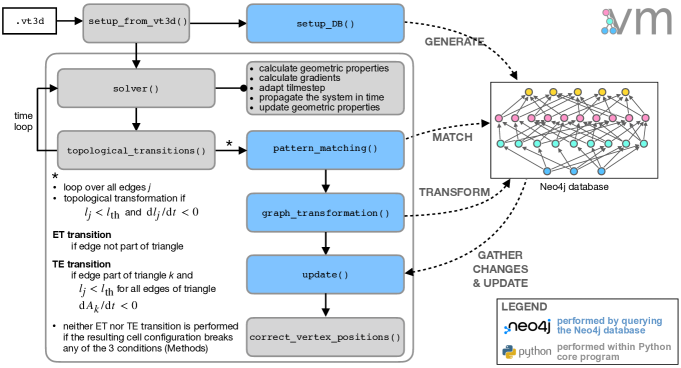
Figure S4: The algorithm underlying neoVM. A 3D cell aggregate is set up from an input .vt3d file by function setup_from_vt3d() and then converted into a graph database, set up in Neo4j by function setupDB(). These initialization steps then followed by a time loop, which iterates between solver() and topological_transitions() functions. The function solver() calculates geometric properties of cells and the associated gradients (i.e., conservative forces) and propagates the system forward in time. The function topological_transitions() loops over all cell edges to find those that meet criteria for topological transitions. For edges that meet these criteria, topological transitions are performed through pattern matching and graph transformations (functions pattern_matching() and graph_transformation(), respectively), applied directly to the graph database. Finally, the tissue is updated accordingly by function update() and positions of vertices involved in the topological transformation are corrected by function correct_vertex_positions().

Figure S4 shows the schematic of neoVM’s architecture. The program is initialized by reading the initial geometry and topology of the cell network from an input .vt3d file and storing them into an object t of class tissue. In particular, this object stores lists of vertex, edge, polygon, and cell objects, which encode $\underline{\boldsymbol{r}}_{i}$, $\underline{\boldsymbol{e}}_{j}$, $\underline{\boldsymbol{p}}_{k}$, and $\underline{\boldsymbol{c}}_{l}$, respectively, in a tabular form. This is followed by generating an object db of class database, which connects to an empty Neo4j database and fills it with the tissue data according to the rules of the GVM’s metagraph, using function setup_DB().

The initialization is followed by a time loop, which propagates the system forward in time by time steps $\Delta t$. At each time step, the dynamical system [Eq. (5)] is integrated between $t$ and $t+\Delta t$ [function solver()] and the program checks whether any of the edges in the cell network meets contitions for topological transitions [function topological_transitions()]. In particular, edge $j$ undergoes an ET transition if it is shorter than a threshold length $l_{\rm th}$ and the rate of change of its length is negative (${\rm d}l_{j}/{\rm d}t<0$), i.e., the edge is contracting. If the edge happens to be part of a triangle, a TE transition is performed on the triangle if, additionally, all edges of the triangle are shorter than $l_{\rm th}$ and the area of the triangle is decreasing (${\rm d}A_{k}/{\rm d}t<0$).

For every edge/triangle, subject to a topological transition, the core program sends a sequence of Cypher queries to the Neo4j graph database. These queries (i) perform pattern matching to isolate a subgraph relevant for the particular transformation being performed, and (ii) perform graph transformation on that subgraph. After graph transformations, vertex positions are displaced such that the lengths of the newly created edges (edges $e_{7}$, $e_{8}$, and $e_{9}$ in Fig. 1) are on the order of $l_{\rm new}\ll 1$. Finally, the local structure of the arrays, encoding $\underline{\boldsymbol{r}}_{i}$, $\underline{\boldsymbol{e}}_{j}$, $\underline{\boldsymbol{p}}_{k}$, and $\underline{\boldsymbol{c}}_{l}$, (stored in object t) are updated according to the applied transformations. This is done by converting the altered part of the knowledge graph back into the array format using function update().

Data availability

Data supporting the findings of this manuscript are available from the corresponding author upon reasonable request. neoVM is available in an online repository [52]. A reporting summary for this Article is available as a Supplementary Information file.

Author Contributions

M.K. conceived the project; T.S. and M.K. developed graph transformations; T.S. carried out the numerical work; T.S. analyzed the data; T.S. and M.K. wrote the paper.

Competing interests

The authors declare no competing interests.

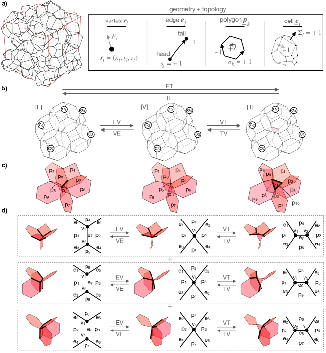
Figure 1: Geometry and topology of cell aggregates. a Cell aggregate is modeled by a space-filling packing of polyhedral cells. Cell shapes are parametrized by vertex positions $\boldsymbol{r}_{i}$, which move according to mechanical forces $\boldsymbol{F}_{i}$. Topology of the cell network is specified by lists $\underline{\boldsymbol{e}}_{j}$, $\underline{\boldsymbol{p}}_{k}$, and $\underline{\boldsymbol{c}}_{l}$ [Eqs. (2)-(4)], which store head and tail vertices of edges, oriented edges within polygons, and oriented polygons within cells, respectively. b EV transition merges vertices of an edge into a single vertex, whereas VT transition resolves a vertex into a triangle. TV and VE transitions are inverse transitions of EV and VT transitions, respectively. c Polygons involved in topological transitions from panel b. d Polygons and edges involved in topological transitions from panel b. 3D topological transitions can be viewed as triple 2D topological transitions, where only edges and polygons are involved.

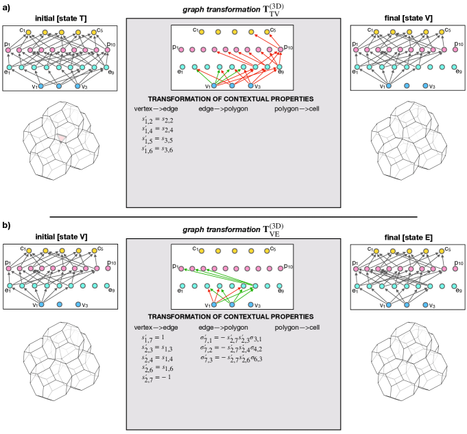
Figure S2: Graph transformations of TV and VE transitions. (panels a and b, respectively). Graphs in the left and the right column correspond to the initial and the final cell configuration, respectively. Gray arrows represent relationships labeled IS_PART_OF. The graphs in the middle column show graph transformations, which include green and red relationships, indicating relationship creations and deletions, respectively. Additionally, the graph transformation specifies property values of the newly created relationships. In each graph, the node indices increase from left to right in unit steps.

References

- [1] T. Lecuit and P.-F. Lenne, Cell surface mechanics and the control of cell shape, tissue patterns and morphogenesis, Nat. Rev. Mol. Cell Biol. 8, 633 (2007).
- [2] T. E. Angelini, E. Hannezo, X. Trepat, M. Marquez, J. J. Fredberg, and D. A. Weitz, Glass-like dynamics of collective cell migration, Proc. Natl. Acad. Sci. USA 108, 4714 (2011).
- [3] J.-A. Park et al., Unjamming and cell shape in the asthmatic airway epithelium, Nat. Mater. 14, 1040 (2015).
- [4] A. Mongera, P. Rowghanian, H. J. Gustafson, E. Shelton, D. A. Kealhofer, E. K. Carn, F. Serwane, A. A. Lucio, J. Giammona, and O. Campàs, A fluid-to-solid jamming transition underlies vertebrate body axis elongation, Nature 561, 401 (2018).
- [5] R. Etournay, M. Popović, M. Merkel, A. Nandi, C. Blasse, B. Aigouy, H. Brandl, G. Myers, G. Salbreux, F. Jülicher, and S. Eaton, Interplay of cell dynamics and epithelial tension during morphogenesis of the Drosophila pupal wing, eLife 4, e07090 (2015).
- [6] D. E. Discher, P. Janmey, and Y.-L. Wang, Tissue Cells Feel and Respond to the Stiffness of Their Substrate, Science 310, 1139 (2005).
- [7] V. F. Fiore, M. Krajnc, F. Garcia Quiroz, J. Levorse, H. A. Pasolli, S. Y. Shvartsman, and E. Fuchs, Mechanics of a multilayer epithelium instruct tumour architecture and function, Nature 585, 433 (2020).
- [8] J. T. Blankenship, S. T. Backovic, J. S. P. Sanny, O. Weitz, and J. A. Zallen, Multicellular rosette formation links planar cell polarity to tissue morphogenesis, Dev. Cell 11, 459 (2006).
- [9] A. Martin, M. Kaschube, and E. F. Wieschaus, Pulsed contractions of an actin–myosin network drive apical constriction, Nature 457, 459 (2009).
- [10] M. Rauzi, U. Krzic, T. E. Saunders, M. Krajnc, P. Ziherl, L. Hufnagel, and M. Leptin, Embryo-scale tissue mechanics during Drosophila gastrulation movements, Nat. Commun. 6, 8677 (2015).
- [11] S. Streichan, M. F. Lefebvre, N. Noll, E. F. Wieschaus, and B. I. Shraiman, Global morphogenetic flow is accurately predicted by the spatial distribution of myosin motors, eLife 7, e27454 (2018).
- [12] T. Stern, S. Y. Shvartsman, and E. F. Wieschaus, Template-based mapping of dynamic motifs in tissue morphogenesis, PLoS Comput. Biol. 16, e1008049 (2020).
- [13] T. Stern, S. Y. Shvartsman, and E. F. Wieschaus, Deconstructing gastrulation at single-cell resolution, Curr. Biol. 32, 1861 (2022).
- [14] C. Bertet, L. Sulak, and T. Lecuit, Myosin-dependent junction remodelling controls planar cell intercalation and axis elongation, Nature 429, 667 (2004).
- [15] M. Rauzi, P. Verant, T. Lecuit, and P.-F. Lenne, Nature and anisotropy of cortical forces orienting Drosophila tissue morphogenesis, Nat. Cell Biol. 10, 1401 (2008).
- [16] M. Rauzi, P.-F. Lenne, and T. Lecuit, Planar polarized actomyosin contractile flows control epithelial junction remodelling, Nature 468, 1110 (2010).
- [17] T. Lecuit, P.-F. Lenne, E. Munro, Force generation, transmission, and integration during cell and tissue morphogenesis, Annu. Rev. Cell Dev. Biol. 27, 157 (2011).
- [18] T. Lecuit and A. S. Yap, E-cadherin junctions as active mechanical integrators in tissue dynamics , Nat. Cell Biol. 17, 533 (2015).
- [19] S. Curran, C. Strandkvist, J. Bathmann, M. de Gennes, A. Kabla, G. Salbreux, and B. Baum, Myosin II Controls Junction Fluctuations to Guide Epithelial Tissue Ordering, Dev. Cell 43, 480 (2017).
- [20] M. Krajnc, Solid–fluid transition and cell sorting in epithelia with junctional tension fluctuations, Soft Matter 13, 3209 (2020).
- [21] M. Krajnc, S. Dasgupta, P. Ziherl, and J. Prost, Fluidization of epithelial sheets by active cell rearrangements, Phys. Rev. E 98, 022409 (2018).
- [22] M. Krajnc, T. Stern, and C. Zankoc, Active Instability and Nonlinear Dynamics of Cell-Cell Junctions, Phys. Rev. Lett. 127, 198103 (2021).
- [23] M. F. Staddon, K. E. Cavanaugh, E. M. Munro, M. L. Gardel, and S. Banerjee, Mechanosensitive junction remodeling promotes robust epithelial morphogenesis, Biophys. J. 19, 1739 (2019).
- [24] K. E. Cavanaugh, M. F. Staddon, T. A. Chmiel, R. Harmon, S. Budnar, S. Banerjee, and M. L. Gardel, Force-dependent intercellular adhesion strengthening underlies asymmetric adherens junction contraction, Curr. Biol. 32, 1986 (2022).
- [25] R. Sknepnek, I. Djafer-Cherif, M. Chuai, C. Weijer, and S. Henkes, Generating active T1 transitions through mechanochemical feedback, eLife 12, e79862 (2023).
- [26] R. Alert and X. Trepat, Physical Models of Collective Cell Migration, Annu. Rev. Condens. Matter Phys. 11, 77 (2020).
- [27] F. Graner, J. A. Glazier, Simulation of biological cell sorting using a two-dimensional extended Potts model, Phys. Rev. Lett. 69, 2013 (1992).
- [28] J. A. Glazier and F. Graner, Simulation of the differential adhesion driven rearrangement of biological cells, Phys. Rev. E 47, 2128 (1993).
- [29] M. H. Swat, G. L. Thomas, J. M. Belmonte, A. Shirinifard, D. Hmeljak, and J. A. Glazier, Multi-scale modeling of tissues using CompuCell3D, Methods Cell Biol. 110, 325 (2012).
- [30] D. Bi, J. H. Lopez, J. M. Schwarz, and M. L. Manning, A density-independent glass transition in biological tissues, Nat. Phys. 11, 1074 (2015).
- [31] M. Misra, B. Audoly, I. G. Kevrekidis, and S. Y. Shvartsman, Biophys. J. 110, 1670 (2016).
- [32] D. Bi, X. Yang, M. C. Marchetti, and M. L. Manning, Motility-driven glass and jamming transitions in biological tissues, Phys. Rev. X 6, 021011 (2016).
- [33] D. L. Barton, S. Henkes, C. J. Weijer, and R. Sknepnek, Active vertex model for cell-resolution description of epithelial tissue mechanics, PLoS Comp. Biol. 13, e1005569 (2017).
- [34] R. Mueller, J. M. Yeomans, and A. Doostmohammadi, Emergence of Active Nematic Behavior in Monolayers of Isotropic Cells, Phys. Rev. Lett. 122, 048004 (2019).
- [35] S. Kim, M. Pochitaloff, G. A. Stooke-Vaughan, and O. Campàs, Embryonic tissues as active foams, Nat. Phys. 17, 859 (2021).
- [36] H. Honda, M. Tenemura, and T. Nagai, A three-dimensional vertex dynamics cell model of space-filling polyhedra simulating cell behavior in a cell aggregate, J. Theor. Biol. 226, 439 (2004).
- [37] R. Farhadifar, J. C. Röper, B. Aigouy, S. Eaton, and F. Jülicher, The influence of cell mechanics, cell-cell interactions, and proliferation on epithelial packing, Curr. Biol. 17, 2095 (2007).
- [38] A. G. Fletcher, M. Osterfield, R. E. Baker, and S. Y. Shvartsman, Vertex models of epithelial morphogenesis, Biophys. J. 106, 2291 (2014).
- [39] S. Alt, P. Ganguly, and G. Salbreux, Vertex models: from cell mechanics to tissue morphogenesis, Philos. Trans. R. Soc. Lond. B Biol. Sci. 372, 20150520 (2017).
- [40] https://github.com/DamCB/tyssue.
- [41] G. R. Mirams, C. J. Arthurs, M. O. Bernabeu, R. Bordas, J. Cooper, A. Corrias, Y. Davit, S.-J. Dunn, A. G. Fletcher, D. G. Harvey et al., Chaste: An open source C + + library for computational physiology and biology, PLoS Comput. Biol. 9, e1002970 (2013).
- [42] D. M. Sussman, cellGPU: Massively parallel simulations of dynamic vertex models, Comput. Phys. Commun. 219, 400 (2017).
- [43] https://github.com/ZhangTao-SJTU/tvm.
- [44] S. Okuda, Y. Inoue, M. Eiraku, Y. Sasai, and T. Adachi, Reversible network reconnection model for simulating large deformation in dynamic tissue morphogenesis, Biomech. Model. Mechanobiol. 12, 627 (2013).
- [45] S. Okuda, T. Miura, Y. Inoue, T. Adachi, and M. Eiraku, Combining turing and 3D vertex models reproduces autonomous multicellular morphogenesis with undulation, tubulation, and branching, Sci. Rep. 8, 2386 (2018).
- [46] L. Sui, S. Alt, M. Weigert, N. Dye, S. Eaton, F. Jug, E. W. Myers, F. Jülicher, G. Salbreux, and C. Dahmann, Differential lateral and basal tension drive folding of Drosophila wing discs through two distinct mechanisms, Nat. Commun. 9, 4620 (2018).
- [47] J. Rozman, M. Krajnc, and P. Ziherl, Collective cell mechanics of epithelial shells with organoid-like morphologies, Nat. Commun. 11, 3805 (2020).
- [48] J. Rozman, M. Krajnc, and P. Ziherl, Morphologies of compressed active epithelial monolayers, Eur. Phys. J. E 44, 1 (2021).
- [49] S. Okuda and K. Sato, Polarized interfacial tension induces collective migration of cells, as a cluster, in a 3D tissue, Biophys. J. 121, 1856 (2022).
- [50] T. Zhang and J. M. Schwarz, Topologically-protected interior for three-dimensional confluent cellular collectives, Phys. Rev. Res. 4, 043148 (2022).
- [51] E. Lawson-Keister, Tao Zhang, and M. L. Manning, Differences in boundary behavior in the 3D vertex and Voronoi models, arXiv: 2306.03987.
- [52] https://gitlab.com/ijskrajncgroup1/neovm.
- [53] https://neo4j.com/product.
- [54] X. Trepat, M. R. Wasserman, T. E. Anglelini, E. Millet, D. A. Weitz, J. P. Butler, and J. J. Fredberg, Physical forces during collective cell migration, Nat. Phys. 5, 426 (2009).
- [55] J. Derganc, S. Svetina, and B. Žekš, Equilibrium mechanics of monolayered epithelium, J. Theor. Biol. 260, 333 (2009).
- [56] M. L. Manning, R. A. Foty, M. S. Steinberg, and E.-M. Schoetz, Coaction of intercellular adhesion and cortical tension specifies tissue surface tension, Proc. Natl. Acad. Sci. USA 107, 12517 (2010).
- [57] E. Hannezo, J. Prost, and J.-F. Joanny, Theory of epithelial sheet morphology in three dimensions, Proc. Natl. Acad. Sci. USA 111, 27 (2013).
- [58] D. Weaire and M. A. Fortes, Networklike Propagation of Cell-Level Stress in Sheared Random Foams, Adv. Phys. 43, 685 (1994).
- [59] D. A. Reinelt and A. M. Kraynik, Simple shearing flow of a dry Kelvin soap foam, J. Fluid Mech. 311, 327 (1996).
- [60] H. W. Schwarz, Rearrangements in polyhedric foam, Recl. Trav. Chim. Pays-Bas 84, 771 (1965).
- [61] J.-F. Rupprecht, K. H. Ong, J. Yin, A. Huang, A. P Singh, S. Zhang, W. Yu, T. E Saunders, Geometric constraints alter cell arrangements within curved epithelial tissues, Mol. Biol. Cell 28, 3582 (2017).
- [62] P. Gómez Gálvez et al., Scutoids are a geometrical solution to three-dimensional packing of epithelia, Nat. Commun. 9, 2960 (2018).
- [63] H. Paulheim, Knowledge Graph Refinement: A Survey of Approaches and Evaluation Methods, Semant. Web 8, 489 (2017).
- [64] https://neo4j.com/docs/cypher-manual/current/introduction/cypher_overview/.
- [65] M. Krajnc, J. Deuser, J. Lampič, T. Sarkar, and T. Stern, In preparation.