Fast, low-loss all-optical phase modulation in warm rubidium vapour

Abstract

High-speed switching with low loss would be a versatile tool for photonic quantum technologies, with applications in state generation, multiplexing, and the implementation of quantum gates. Phase modulation is one method of achieving this switching, but existing optical phase modulators either achieve high bandwidth or low loss, but not both. We demonstrate fast ($100\text{\,}\mathrm{MHz}$ bandwidth), low-loss ($74(2)\text{\,}\mathrm{\char 37\relax}$ transmission) phase shifting ($\Delta\phi=($0.90(5)\text{\,}$)\pi$) in a signal field, induced by a control field, and mediated by the two-photon $5S_{1/2}\rightarrow{}5P_{3/2}\rightarrow{}5D_{5/2}$ transition in ⁸⁷Rb vapour. We discuss routes to enhance both performance and scalability for application to a range of quantum and classical technologies.

I Introduction

Photonics has revolutionised telecommunications since the development of fibre optics in the 1980s. Photonic data buses are supplanting electronics in high performance computing [1], and more recently photonic platforms for machine learning are emerging [2]. Looking forwards, photonics can provide a platform for communication with enhanced security by quantum key distribution [3] and support the transfer of quantum information between nodes [4]. All of these applications require high speed switching which can be achieved by phase modulation of an optical signal, and fibre-integrated electro-optical modulators are commercially mature. Nevertheless the insertion losses of these devices (typically $3\text{\,}\mathrm{dB}$) add a practical overhead: mitigating these losses requires increased input power, intermediate amplifiers, and waste heat management [5]. Further, increasing demand on switching speeds could lead to the obsolescence of existing semiconductor-based telecommunications devices [6]. More efficient technologies for optical modulation are thus desirable across a range of application areas.

The primary motivation for our work in this paper is in the area of photonic quantum computing [7], where engineered non-classical optical states are used to solve computational problems that are intractable with classical (i.e. non-quantum) resources. Photonic quantum computing is appealing for a number of reasons, including room-temperature operation of all or many components, high clock-rates, high connectivity, insensitivity to stray fields and modular construction. But a key technical challenge remains: the requirement to switch and dynamically re-route photons with high speed and extremely low loss. This is an essential stage in a variety of processes for photonic quantum computing, such as implementing: loop memories [8, 9], synchronisation [10] or multiplexing [11, 12, 13] of single photon sources and demultiplexing for graph state generation [14]. Amplification destroys quantum coherence and so cannot be used to mitigate losses in a quantum system. The lifetime of photons in a waveguide is limited, and so high bandwidth is required for scalability. For these reasons, quantum systems have extremely stringent tolerances for speed and loss [15], which motivates an exploration of alternative platforms that could ultimately deliver better performance than current fibre-integrated electro-optic modulators.

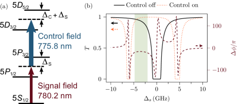
Figure 1: (a) Ladder scheme used for phase modulation of weak signal field (red) by presence of strong control field (blue) detuned from $5S_{1/2}\rightarrow{}5P_{3/2}$ and $5P_{3/2}\rightarrow{}5D_{5/2}$ transitions by $\Delta_{s}$ and $\Delta_{c}$ respectively. (b) Transmission with control off (black, solid) and on (orange, dotted) and phase shift (red, dashed) through ⁸⁷Rb vapour for various $\Delta_{s}$, as determined by the theoretical model described in the main text. Control detuning is fixed at $\Delta_{c}=$-1.6\text{\,}\mathrm{GHz}$$. We identify the experimental region of interest (shaded), where there is low-loss for control on and off, as well as a high phase shift. Note also the two-photon absorption feature at $\Delta_{s}=$-6\text{\,}\mathrm{GHz}$$, which is away from $\Delta_{s}=-\Delta_{c}$ due to the a.c. Stark-shift.

In this letter, we describe and demonstrate efficient, all-optical phase modulation of light. Ideal implementation of phase modulation (a phase shift of $\pi$ radians with no loss) would be equivalent to implementation of an optical switch, by embedding the phase modulator in one arm of a Mach-Zehnder interferometer. Our scheme, depicted in Fig. 1 (a), takes advantage of the $5S_{1/2}\rightarrow{}5P_{3/2}\rightarrow{}5D_{5/2}$ two-photon transition in ⁸⁷Rb. This is the same transition used in electromagnetically-induced transparency (EIT) optical control [16, 17] and memory [18] schemes. A weak signal field, detuned from resonance with the $5S_{1/2}\rightarrow{}5P_{3/2}$ transition by frequency $\Delta_{s}$, counter-propagates through a ⁸⁷Rb vapour cell with a high-intensity, pulsed control field. This control field is detuned from resonance with the $5P_{3/2}\rightarrow{}5D_{5/2}$ transition by frequency $\Delta_{c}$, and its presence induces a change in the susceptibility of the ⁸⁷Rb, as experienced by the signal. Hence, the control field modulates the phase of the signal field as it traverses the vapour cell. We will first outline a simple theoretical model of this phase modulation, before describing the experimental results for a continuous wave (CW) and pulsed signal field.

II Theory of optical phase modulation in atoms

In general, light with wavenumber $k$ travelling through a medium of length $L$ will accumulate a phase

$$\phi=kL\real(\sqrt{1+\chi}),$$ (1)

where $\chi$ is the susceptibility of the medium. The transmission of the medium is given by $T=\exp(-\alpha L)$, where $\alpha$ is the extinction coefficient,

$$\alpha=-2k\imaginary(\sqrt{1+\chi}).$$ (2)

The difference in phase between two possible paths is the phase shift ($\Delta\phi$). The phase shift and loss experienced by a field, $E$, can be extracted by interference with the original field. We perform such interference using a Mach-Zehnder interferometer, so at the two output ports we have fields $E_{1,2}$, whose amplitudes are

$$\begin{split}E_{1}&=\sqrt{T}E\cos(\Delta\phi/2),\\ E_{2}&=\sqrt{T}E\sin(\Delta\phi/2).\end{split}$$ (3)

We can then extract $\Delta\phi$ and $T$ from measurement of the two fields’ intensities.

The phase shift through the ⁸⁷Rb vapour can be understood as a function of $\chi$, which in turn depends on the properties of both the control field and the vapour (specifically its density and temperature). We model $\chi$ by numerical solution of the Maxwell-Bloch equations [19, 20, 21, 22, 23] (see supplementary material), allowing us to identify suitable signal and control detunings where we can achieve both high phase shift and low loss. We consider a simplified model in which the system is in a steady state and the field across the medium is uniform – however, both of these assumptions may lead to disparity with experimental results where we have a pulsed control field and observe a broadening of the Stark shift across the mode due to the radial variation of the fields.

The phase shift and transmission for a representative experiment is shown in Fig. 1 (b), and can be used to identify a region of low loss and high phase shift (grey shading, $\Delta_{s}=$-4.8\text{\,}\mathrm{GHz}-2\text{\,}\mathrm{GHz}$$). In this region there is a flat, non-zero phase shift of $\Delta\phi=-15\pi$, and since it far detuned from both the single- and two-photon absorption features ($\Delta_{c}=$1.6\text{\,}\mathrm{GHz}$$) it also exhibits low loss. For this calculation the CW control power is $11\text{\,}\mathrm{W}$, which is comparable to the peak power of the $47\text{\,}\mathrm{nJ}$, $4\text{\,}\mathrm{ns}$ FWHM duration control pulses used in Section III. The signal is also taken to be CW with negligible power. Both beams have a $125\text{\,}\mathrm{\SIUnitSymbolMicro m}$ waist and travel through a cell of length $7\text{\,}\mathrm{cm}$ at a temperature of $95\text{\,}\mathrm{\SIUnitSymbolCelsius}$. It is assumed the atoms are equally spread across the Zeeman states of both the $F=2$ and $F=1$ ground states at room temperature [24].

III Phase modulation of a CW signal field

First we discuss the experimental implementation in which a CW signal field is modulated by a pulsed control field. This allows the demonstration of a phase shift that varies with the signal detuning $\Delta_{s}$ for a fixed control detuning $\Delta_{c}$. The experiment is shown in Fig. 2, and uses the CW signal preparation in the upper dashed box. The CW signal is generated by an external cavity diode laser (MOGLabs CEL) whose frequency is scanned across the region of interest shown in Fig. 1. Control pulses are generated by pulse carving, amplifying and frequency doubling a pulsed telecomms laser operating near $1552\text{\,}\mathrm{nm}$ (details are given in the supplementary material). The control pulses are square, with $4\text{\,}\mathrm{ns}$ duration and $47\text{\,}\mathrm{nJ}$ pulse energy. The signal field average power is $1.6\text{\,}\mathrm{mW}$. Since the timescale of the pulses is much shorter than that of the signal frequency scan, we assume that $\Delta_{s}$ is effectively constant for each control pulse.

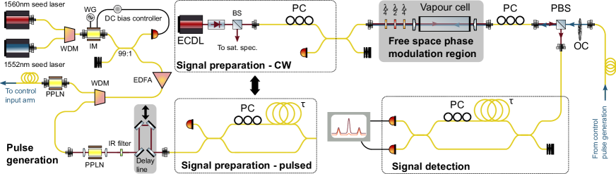
Figure 2: Experimental setup, showing control and signal fields counter-propagating through ⁸⁷Rb vapour cell in free space, the generation scheme for pulses and CW signal field, and detection region. In the CW case, a beamsplitter (BS) is used to calibrate the external cavity diode laser (ECDL) by saturation absorption spectroscopy of Rb and in the pulsed case an optical chopper (OC) is inserted to modulate the control pulses. Signal and control pulses can be generated by combining telecomms seed lasers with a wavelength-division multiplexer (WDM) before pulse carving using a LiNbO₃ intensity modulator (IM) before amplification by erbium-doped fibre amplifier (EDFA). The two wavelengths are separated at a second WDM, before frequency doubling at periodically poled LiNbO₃ crystals (PPLN) and sent to the experiment. A delay line is used to synchronise the arrival time of signal and control pulses. Further details of the pulse generation are given in the supplementary material. Polarisation controllers (PC) and waveplates ($\lambda/2$, $\lambda/4$) ensure that the polarisation of the fields is $\sigma^{+}$ circularly polarised at the vapour cell, and separates the fields at a polarising beam splitter (PBS) for phase-sensitive signal detection by a Franson interferometer. The purpose of fibre delay lines with duration $\tau$ is explained in the main text.

The signal field counter propagates with control pulses through the $7\text{\,}\mathrm{cm}$ long, isotopically pure ⁸⁷Rb vapour cell (Precision Glassblowing) heated to $97.6\text{\,}\mathrm{\SIUnitSymbolCelsius}$. Half- and quarter-waveplates are set so that the light is circularly polarised, maximising the strength of the interaction  [25]. Following this, the signal field is separated into the detection region, which consists of a Franson interferometer [26] (see Fig. 3) with polarisation control used to maximise the fringes. Note that the interferometer has a free spectral range of $200\text{\,}\mathrm{MHz}$, however for simplicity we consider only values of $\Delta_{s}$ where the output through port 1 is maximised. A phase shift is detected by a change in the intensity at each output.

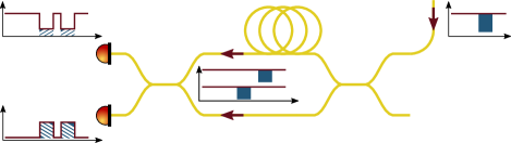
Figure 3: Time-bin interferometer detection scheme for CW operation. Regions of the signal overlapping with a control pulse in the cell are shaded blue. Blue hashing indicates regions of interference at the output.

We observe fringes described by Eqn. 3 at the interferometer output, from which we extract $\Delta\phi$ and $T$ for a range of signal detunings and control pulses detuned by $\Delta_{c}=$1.6\text{\,}\mathrm{GHz}$$. The results are shown in Fig. 4. We observe that for $\Delta_{s}$ close to zero there is increased absorption due to broadening of the single-photon resonance, and that there is significant absorption from the two-photon effect around $\Delta_{s}=$-3\text{\,}\mathrm{GHz}$$. We identify a range of $\Delta_{s}=$-1.85\text{\,}\mathrm{GHz}-1.5\text{\,}\mathrm{GHz}$$ where the transmission is highest and the phase shift is relatively flat. We achieve a phase shift $\Delta\phi/\pi=$0.90(5)\text{\,}$$ with end-to-end transmission $T=$74(2)\text{\,}\mathrm{\char 37\relax}$$, which includes the insertion loss through the vapour cell of $4.5\text{\,}\mathrm{\char 37\relax}$.

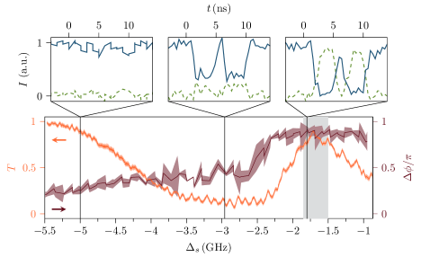
Figure 4: The upper three plots show the signal arriving at detectors 1 (green, dashed) and 2 (blue, solid) for various values of $\Delta_{s}$ (cf. Fig. 3). In each of these traces, $t=0$ corresponds to the detection time of the control pulse. Analysis of these peaks allows us to determine the transmission through the vapour cell ($T$) as well as the phase shift ($\Delta\phi$), both of which are shown for the full scan of $\Delta_{s}$ in the second row.

IV Phase modulating a pulsed signal field

In this section we discuss the phase modulation of a $\sim 100$ MHz-bandwidth pulsed signal field, as required for clocked photonic systems. Signal pulses are generated by the same means as for control pulses, as was described in the previous section and detailed in the supplementary material. The same EDFA is used simultaneously for both wavelengths, which reduces the total power in the control. Signal field pulses are split, with a time delay of $\tau=$10\text{\,}\mathrm{ns}$$, as shown in the lower dashed box of Fig. 2. The delay line is used to ensure that both signal and control pulses arrive at the cell together, such that the control overlaps with only the second pulse. The control beam is chopped at $1\text{\,}\mathrm{kHz}$ to allow extraction of the control-induced phase shift on a time-scale fast compared to the interferometer drift. The optical amplifier gain is now divided between signal and control fields, which reduces the available control power and consequently the achievable phase shift.

We set $\Delta_{c}=$2\text{\,}\mathrm{GHz}$$, and ramp $\Delta_{s}$ over a range $-2\text{\,}\mathrm{GHz}0\text{\,}\mathrm{GHz}$ at a frequency of $1\text{\,}\mathrm{Hz}$, much slower than the chopper frequency. Ramping $\Delta_{s}$ allows the single-photon absorption line to be resolved when the control is off, so that the stability of the laser can be monitored, and $\Delta_{s}$ can be determined precisely. Any signal pulses that experience a partially chopped control are discarded from the analysis. As the chopper frequency is three orders of magnitude larger than the signal ramp frequency, the signal laser frequency is roughly constant across the control pulses contained within a single window of the chopper.

The results for modulation of the pulsed signal field are shown in Fig. 5. The cell is again held at $97.6\text{\,}\mathrm{\SIUnitSymbolCelsius}$, with control pulse energy of $33\text{\,}\mathrm{nJ}$, signal pulse energy of $200\text{\,}\mathrm{pJ}$, $\Delta_{c}=$2\text{\,}\mathrm{GHz}$$, $\Delta_{s}=-$1.9\text{\,}\mathrm{GHz}$$, and pulse duration $4\text{\,}\mathrm{ns}$. The switch of the interferometer output from detector 2 to detector 1 is due to the presence of the control field, and is a clear indicator of phase modulation. Comparison of the two right hand peaks shows that the control pulses are changing the shape and magnitude of the signal pulse, due to a combination of absorption and dispersion induced by the control.

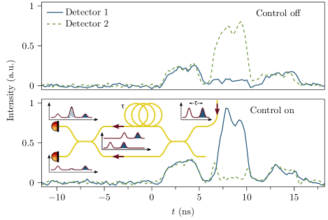
Figure 5: Demonstration of phase modulation for pulsed control and signal. We show the interferometer output for control off (top panel) and on (bottom panel) for signal pulses as described in the main text. Here we set $t=0$ as the time that the first pulse arrives. Note the change in the central peak between the control on and off, corresponding to $\Delta\phi/\pi=$0.53(6)\text{\,}$$ The inset shows how we interpret the three peaks arriving in at the signal detection arm shown in Fig. 2, with polarisation controllers omitted for clarity. A pulse which has encountered a control pulse in the vapour cell is indicated by blue shading. Interference on the central peak at the output is indicated by blue-white hashing, and is used to extract transmission and phase information as in the CW case.

The average transmission and phase shift across these pulses is calculated by integration. This yields a transmission of $T=$81(6)\text{\,}\mathrm{\char 37\relax}$$, including vapour cell insertion loss, and phase shift of $\Delta\phi/\pi=$0.53(6)\text{\,}$$. As the control pulse is the same duration as the signal pulse, then the signal pulse does not experience a uniform control intensity distribution in time. The incomplete temporal overlap reduces the phase modulation effect, as can be seen in the edges of the the detector 2 peak when the control pulse is on in Fig. 5.

V Conclusion

We have demonstrated low-loss, all-optical phase modulation operating on the timescale of nanoseconds. Our scheme utilises the change in susceptibility of warm ⁸⁷Rb vapour in the presence of a strong control field, inducing a phase shift in a weak signal field. We are able to demonstrate phase shifts close to $\Delta\phi=\pi$, the critical value required for optical switching. Our theoretical model predicts that reaching $|\Delta\phi|>10\pi$ is possible with low loss, and that simultaneously increasing the temperature, control power and control detuning is predicted to further improve the performance [27].

However a complete description of the phase modulation behaviour, accounting for the time-variation of the control field, as well as the dependence on the population of the various hyperfine states would allow further improvements to the scheme [28]. This may come in the form of different detunings, or optimisation of the hyperfine occupation by optical pumping [18].

We propose that improvement to phase shift and transmission can be made by implementing the phase modulation scheme inside a hollow core optical fibre [29] where the core is filled with ⁸⁷Rb vapour to realise an in-fibre vapour cell [30, 31, 32]. This would allow for significantly higher intensity, and hence higher phase shift, of the control field, due to the small ($\sim$1000\text{\,}{\mathrm{\SIUnitSymbolMicro m}}^{2}$$) size of the mode which can be maintained over lengths of optical fibre much greater than the Rayleigh range. Such a device would have potential for scalability, due to ability to easily integrate with other optical fibre systems [33]. An alternative route to enhancement is by implementation in an optical cavity, where the interaction of the control field is increased by a factor of the cavity finesse [34, 35, 36]. This is particularly appealing for microresonators where high quality factors ($Q>10^{6}$) are readily achievable [37, 38, 39, 40, 41].

Finally, we suggest that phase modulation at other wavelengths may be possible by applying our same scheme at other wavelengths, particularly those that would be compatible with existing telecommunication infrastructure. Of particular interest may be the $5S_{1/2}\rightarrow{}5P_{3/2}\rightarrow{}4D_{5/2}$ transition also in ⁸⁷Rb, which has recently been used to demonstrate an EIT memory for classical light [42] and single photons [43]. Here, the signal field is on the $5P_{3/2}\rightarrow{}4D_{5/2}$ transition at $1529\text{\,}\mathrm{nm}$, which is close to the telecommunication C-band.

VI Supplementary material

VI.1 Equations of motion

Here we derive the equations of motion for the Rb atoms in the presence of signal and control fields. This follows the similar derivations for the off-resonant cascaded absorption (ORCA) ladder scheme [23] or the derivations for a $\Lambda$-type Raman memory [21]. We begin with the Heisenberg equation

$$\partial_{t}\rho=i[\mathcal{H},\rho].$$ (4)

where $\rho$ is the density matrix, and $\mathcal{H}$ is the Hamiltonian of the system. We write the latter as

$$\mathcal{H}=\mathcal{H}_{\textnormal{A}}+\mathcal{H}_{\textnormal{AF}}$$ (5)

where we have the atomic Hamiltonian in the absence of any external fields,

$$\mathcal{H}_{\textnormal{A}}=\sum_{j}\hbar\omega_{j}\ket{j}\bra{j}=\sum_{j}\hbar\omega_{j}\rho_{jj}$$ (6)

and the light-atom interaction Hamiltonian

$$\mathcal{H}_{\textnormal{AF}}=-\mathbf{d}\cdot\mathbf{E}.$$ (7)

The electric field is defined as the sum of the signal and control fields ($\mathbf{E}_{s}$ and $\mathbf{E}_{c}$ respectively),

$$\begin{split}\mathbf{E}=&\mathbf{E}_{s}+\mathbf{E}_{c}\\ =&\bm{\nu}_{\textnormal{c}}E_{\textnormal{c}}e^{i\omega_{\textnormal{c}}(t+\frac{z}{c})}+\bm{\nu}^{*}_{\textnormal{c}}E^{*}_{\textnormal{c}}e^{-i\omega_{\textnormal{c}}(t+\frac{z}{c})}\\ &+\bm{\nu}_{\textnormal{s}}E_{\textnormal{s}}e^{i\omega_{\textnormal{s}}(t-\frac{z}{c})}+\bm{\nu}^{*}_{\textnormal{s}}E^{*}_{\textnormal{s}}e^{-i\omega_{\textnormal{s}}(t-\frac{z}{c})},\end{split}$$ (8)

where $\bm{\nu}_{\textnormal{c}}$ and $\bm{\omega}_{\textnormal{c}}$ ($\bm{\nu}_{\textnormal{s}}$ and $\bm{\omega}_{\textnormal{s}}$) are the polarisation vector and angular frequency of the control (signal) fields respectively. The dipole operator $\mathbf{d}$ is given by

$$\begin{split}\mathbf{d}=&\sum_{j,k}\bra{j}\mathbf{d}\ket{k}\rho_{jk}\ +\bra{j}\mathbf{d}\ket{k}^{*}\rho^{\dagger}_{jk}\\ =&\sum_{j,k}\bra{j}\mathbf{d}\ket{k}\ket{j}\bra{k}+\bra{j}\mathbf{d}\ket{k}^{*}\ket{k}\bra{j}.\end{split}$$ (9)

We write the dipole matrix elements in the usual way,

$$d_{jk}=\bra{j}\mathbf{d}\ket{k}.$$ (10)

We will treat the Rb atom as a three level system, so that, $j,k=1,2,3$ (corresponding to the $S$, $P$, and $D$ states of interest respectively), and the operators defined above can be written as $3\times 3$ matrices. We now calculate each matrix element of the Hamiltonian

$$\mathcal{H}_{jk}=\bra{j}\mathcal{H}\ket{k}.$$ (11)

The atomic Hamiltonian has non-zero elements only when $j=k$. The electric dipole interaction has odd parity, and only off-diagonal elements for the electric dipole interaction remain are non-zero. The on-diagonal elements in the density matrix are the populations, and the off-diagonal elements are the coherences. For a weak signal field in which the number of rubidium atoms in the mode is much larger than the number of photons. We can assume that any change in populations of the states are negligible. This means that $\rho_{11}=1$, as virtually the entire atomic population will remain in the ground state, and thus $\rho_{22}$ and $\rho_{33}=0$ as there is negligible population in the upper states. The change in the populations of the states are also negligible and so $\partial_{t}\rho_{11}\ =~{}\partial_{t}\rho_{22}\ =~{}\partial_{t}\rho_{33}\ =~{}0$.

The ground state energy is defined as $\hbar\omega_{1}$ = 0 and it is assumed there is no coupling between the excited states, so that $d_{13}=d_{31}$ = 0. Applying the above assumptions we can write down the matrices

$$\mathcal{H}=\begin{pmatrix}0&-\mathbf{d}_{12}.\mathbf{E}&0\\ -\mathbf{d}_{21}.\mathbf{E}&\hbar\omega_{2}&-\mathbf{d}_{23}.\mathbf{E}\\ 0&-\mathbf{d}_{32}.\mathbf{E}&\hbar\omega_{3}\end{pmatrix},$$ (12)

$$\rho=\begin{pmatrix}1&\rho_{12}&\rho_{13}\\ \rho_{21}&0&\rho_{23}\\ \rho_{31}&\rho_{32}&0\end{pmatrix}.$$ (13)

The angular frequencies are defined as $\omega_{2}=-\omega_{12}$, $\omega_{3}=-\omega_{13}$ and $\omega_{23}=\omega_{2}-\omega_{3}$, where $\omega_{jk}=\omega_{j}-\omega_{k}$ is the transition frequency of the $\ket{j}\xrightarrow{}\ket{k}$ transition.

Doppler broadening can be taken into account by applying the chain rule to the Heisenberg equation of motion, changing the partial differential to a normal time differential [22, 20]. Considering only propagation and motion in the z-direction leads to the equation

$$\frac{\differential\rho(z,t)}{\differential t} =\partial_{t}\rho|_{z}+\partial_{z}\rho|_{t}\frac{\differential z}{\differential t}$$ (14)

$$=-i[\mathcal{H},\rho]-v\partial_{z}\rho$$ (15)

Here $v$ is the velocity of an atom in the $z$ direction. The equations of motion are then [21, 23],

$$\begin{split}\differential_{t}\rho_{13}=&\left(-{\frac{\gamma_{3}}{2}}-i\omega_{13}-v\partial_{z}\right)\rho_{13}\\ &+i\Omega^{*}_{\textnormal{c}}\rho_{12}e^{-i\omega_{\textnormal{c}}(t+\frac{z}{c})},\end{split}$$ (16)

and

$$\begin{split}\differential_{t}\rho_{12}=&\left(-{\frac{\gamma_{2}}{2}}-i\omega_{12}-v\partial_{z}\right)\rho_{12}\\ &+i\kappa_{\textnormal{s}}S+i\Omega_{\textnormal{c}}\rho_{13}e^{i\omega_{\textnormal{c}}(t+\frac{z}{c})}.\end{split}$$ (17)

Here we have introduced the Rabi frequency of the control field

$$\Omega_{\textnormal{c}}={\frac{\mathbf{d}^{*}_{23}\cdot\bm{\nu}_{c}}{\hbar}}E_{\textnormal{c}},$$ (18)

a related parameter for the signal field

$$\kappa_{\textnormal{s}}={\frac{\mathbf{d}_{12}\cdot\bm{\nu}_{s}}{\hbar}},$$ (19)

and we define for convenience

$$S=E_{\textnormal{s}}e^{i\omega_{\textnormal{s}}(t-\frac{z}{c})}$$ (20)

along with $\gamma_{2}$ as the decay rate of the $5P_{3/2}$ state and $\gamma_{3}$ as the decay rate of the $5D_{5/2}$ state.

It is notable that the equation for $\rho_{12}$ has terms for the single-photon transition frequency, the decay rate of the single-photon coherence, and will depend on the single-photon Doppler shift. The equation for $\rho_{13}$ has a term for the two-photon transition frequency, the decay rate of the two-photon coherence, and will depend on the two-photon Doppler shift.

VI.1.1 Fourier transform solution

The equations are solved numerically by Fourier transform from time and space to frequency and reciprocal space. This leads to two equations in frequency and reciprocal space (using a hat to represent the transformed operator)

$$\left({\frac{\gamma_{3}}{2}}+i(\omega+\omega_{13})+ivq\right)\hat{\rho}_{13}(q,\omega)=i\Omega^{*}_{\textnormal{c}}\hat{\rho}_{12}(q+k_{\textnormal{c}},\omega+\omega_{\textnormal{c}}),$$ (21)

$$\left({\frac{\gamma_{2}}{2}}+i(\omega+\omega_{12})+ivq\right)\hat{\rho}_{12}(q,\omega)=i\kappa_{\textnormal{s}}\hat{S}(q,\omega)+i\Omega_{\textnormal{c}}\hat{\rho}_{13}(q-k_{\textnormal{c}},\omega-\omega_{\textnormal{c}}).$$ (22)

We now perform a co-ordinate transform on equation 21 and note that the signal field, $S(q,\omega)$ is a pulse, with most of its energy concentrated around the central frequency $\omega_{\textnormal{s}}$ and central wavevector $k_{\textnormal{s}}$. Therefore, it is a good approximation to define $q=k_{\textnormal{s}}$ and $\omega=\omega_{\textnormal{s}}$. We therefore have that

$$\left({\frac{\gamma_{3}}{2}}+i(\omega_{\textnormal{s}}+\omega_{\textnormal{c}}+\omega_{13})+iv(k_{\textnormal{s}}-k_{\textnormal{c}})\right)\hat{\rho}_{13}(k_{\textnormal{s}}-k_{\textnormal{c}},\omega_{\textnormal{s}}-\omega_{\textnormal{c}})=i\Omega^{*}_{\textnormal{c}}\hat{\rho}_{12}(k_{\textnormal{s}},\omega_{\textnormal{s}}),$$ (23)

$$\left({\frac{\gamma_{2}}{2}}+i(\omega_{\textnormal{s}}+\omega_{12})+ivk_{\textnormal{s}}\right)\hat{\rho}_{12}=i\kappa_{\textnormal{s}}\hat{S}+i\Omega_{\textnormal{c}}\hat{\rho}_{13}.$$ (24)

We now note that that $\omega_{13}=-\omega_{21}-\omega_{32}$, which allows us to write the signal detuning as $\Delta_{\textnormal{s}}=-\omega_{21}+\omega_{\textnormal{s}}$ and control detuning as $\Delta_{\textnormal{c}}=-\omega_{32}+\omega_{\textnormal{c}}$. We can now re-write the above expressions as

$$\left(i{\frac{\gamma_{3}}{2}}-(\Delta_{\textnormal{s}}+\Delta_{\textnormal{c}})-v(k_{\textnormal{s}}-k_{\textnormal{c}})\right)\hat{\rho}_{13}=-\Omega^{*}_{\textnormal{c}}\hat{\rho}_{12},$$ (25)

$$\left(i{\frac{\gamma_{2}}{2}}-\Delta_{\textnormal{s}}-vk_{\textnormal{s}}\right)\hat{\rho}_{12}=-\kappa_{\textnormal{s}}\hat{S}-\Omega_{\textnormal{c}}\hat{\rho}_{13}.$$ (26)

Rearranging equation 25 allows an expression for $\hat{\rho}_{13}$ in terms of $\hat{\rho}_{12}$ to be obtained

$$\hat{\rho}_{13}=\frac{\Omega^{*}_{\textnormal{c}}\hat{\rho}_{12}}{(-i{\frac{\gamma_{3}}{2}}+(\Delta_{\textnormal{s}}+\Delta_{\textnormal{c}})+v(k_{\textnormal{s}}-k_{\textnormal{c}}))}.$$ (27)

Substituting in for $\hat{\rho}_{13}$ in equation 26 and re-arranging provides an expression in terms of $\hat{\rho}_{12}$

$$\hat{\rho}_{12}=\frac{\kappa_{\textnormal{s}}\hat{S}(q,\omega)}{-i{\frac{\gamma_{2}}{2}}+\Delta_{\textnormal{s}}+vk_{\textnormal{s}}-\frac{|\Omega^{2}_{\textnormal{c}}|}{-i{\frac{\gamma_{3}}{2}}+(\Delta_{\textnormal{s}}+\Delta_{\textnormal{c}})+v(k_{\textnormal{s}}-k_{\textnormal{c}})}}.$$ (28)

Next, we define the polarisation density as

$$\mathbf{P}(z,t)=n_{\textnormal{d}}\mathbf{d}_{12}\rho_{12}(z,t),$$ (29)

where $n_{\textnormal{d}}$ is the number density of the vapour. Including Doppler broadening the expression is given by

$$\mathbf{P}(z,t,v)=n_{\textnormal{d}}\mathbf{d}_{12}\int p(v)\rho_{12}(z,t,v)\differential v,$$ (30)

where $p(v)$ is the normal distribution of velocities of particle with mass $m$, and temperature, $T_{\text{cell}}$

$$p(v)=\sqrt{{\frac{m}{2\pi k_{B}T_{\text{cell}}}}}e^{\frac{-mv^{2}}{2k_{B}T_{\text{cell}}}}.$$ (31)

The polarisation density is given by

$$\mathbf{P}(z,\omega)=\epsilon_{0}\chi(\omega)\mathbf{E_{\textnormal{s}}}(z,\omega).$$ (32)

Fourier transforming the above polarisation density relations to the frequency and reciprocal space domains leads to the expressions

$$\hat{\mathbf{P}}(q,\omega,v)=n_{\textnormal{d}}\mathbf{d}_{12}\int p(v)\hat{\rho}_{12}(q,\omega,v)\differential v,$$ (33)

$$\hat{\mathbf{P}}(q,\omega)=\epsilon_{0}\chi(\omega)\mathbf{\hat{E}_{\textnormal{s}}}(q,\omega).$$ (34)

Substituting in for $\hat{\rho}_{12}(v)$ and re-arranging for the susceptibility, $\chi$, leads to the following expression in the steady-state for the three-level system

$$\chi(\omega)={\frac{n_{\textnormal{d}}d_{12}\kappa_{\textnormal{s}}}{\epsilon_{0}}}\int{\frac{p(v)}{-i{\frac{\gamma_{2}}{2}}+\Delta_{\textnormal{s}}+vk_{\textnormal{s}}-\frac{|\Omega^{2}_{\textnormal{c}}|}{-i{\frac{\gamma_{3}}{2}}+(\Delta_{\textnormal{s}}+\Delta_{\textnormal{c}})+v(k_{\textnormal{s}}-k_{\textnormal{c}})}}}\differential v.$$ (35)

This equation can then be solved numerically to find the real and imaginary parts of the susceptibility, by numerically integrating over all velocities. The real and imaginary parts of the susceptibility are related to the complex refractive index by

$$\tilde{n}=n-iK\approx\sqrt{1+\chi}.$$ (36)

Here we have introduced the real numbers $n$ and $K$ to distinguish the real and imaginary parts of the complex refractive index. The former provides information on phase velocity and phase shifts, whereas the latter is the extinction coefficient.

Calculating the refractive index with and without the presence of the control field allows the change in the refractive index, and therefore the change in the phase to be determined using the equation

$$\Delta\phi={\frac{2\pi L}{\lambda_{0}}}(n_{\mathrm{c}}-n_{0})$$ (37)

where $n_{\mathrm{c}}$ ($n_{0}$) is the refractive index with the control field switched on (off), $\lambda_{0}$ is the signal field wavelength, and $L$ is the interaction length. For pulses that are longer than the cell this will be the length of the vapour cell. The absorption coefficient $\alpha$ relates to the extinction coefficient by the following relation

$$\alpha=\frac{4\pi K}{\lambda},$$ (38)

for signal frequency, $f$, extinction coefficient, $K$, and speed of light, $c$. Assuming that the vapour cell is much shorter than the control pulse, then the absorption coefficient experienced by the signal will be uniform across the cell. The transmission in this case is then given by the Beer-Lambert law, giving an exponential decay of the cell transmission

$$T=e^{-\alpha L}.$$ (39)

VI.2 Pulse generation

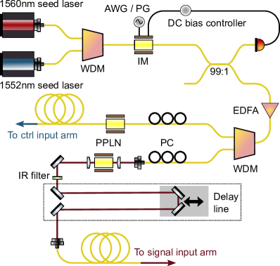
Figure 6: Setup used to generate signal and control pulses. SMF, single-mode fibre; PMF, polarisation-maintaining fibre; FPC, fibre polarisation controller; AWG, arbitary waveform generator; IM, intensity modulator; PD, photodiode; PPLN, periodically poled lithium niobate; WDM, wavelength division multiplexer; EDFA, erbium doped fibre amplifier.

The experimental setup starts with generating two trains of pulses. Strong control pulses at 776 $\mathrm{nm}$ and weak signal pulses at 780.2 $\mathrm{nm}$. The pulse generation scheme is shown in Fig. 6. Two tunable fibre coupled seed lasers in the telecomms C band at 1552 $\mathrm{nm}$ (control) and 1560 $\mathrm{nm}$ (signal) (ID Photonics CoBrite DX1, and Eblana EP1560-0-DM-B05-FM, respectively) are used as seed lasers. Both wavelengths are combined using a wavelength division multiplexer (Oz Optics WDM-12N-111-1552/1560-8/125-PPP-60-3A3A3A-1-1). The seed lasers are pulsed carved using a waveguided Lithium Niobate intensity modulator (EOSpace - AZ-DS5-10-PFA-PFA-LV), stabilised by a DC bias controller (MBC-HER-PD-3A-0V) at the operating point for minimum transmission. Fast electrical pulses are applied by a radio-frequency (RF) pulse generator (Picoquant PPG512) with the repetition rate controlled by an arbitrary waveform generator. This allows a stable train of signal and control pulses to be carved, and the pulse duration can be varied between 600 ps and 4 $\mathrm{ns}$, or longer.

The signal and control pulses are amplified in an Erbium doped fibre amplifier (EDFA). The amplified pulses are then split out using a second wavelength division multiplexer (Oz Optics WDM-12N-111-1552/1560-8/125-SSS-60-3A3A3A-1-1). The 1552 $\mathrm{nm}$ control field passes into a waveguided periodically poled lithium niobate crystal (Covesion WGP-H-1552-40) for frequency doubling to 776 $\mathrm{nm}$. The 1560 $\mathrm{nm}$ signal field is coupled into free-space and is focused into a bulk periodically poled lithium niobate crystal (Covesion MSHG1550-1.0-40) for frequency doubling to 780.2 $\mathrm{nm}$. Any remaining 1560 $\mathrm{nm}$ light is removed by a short-pass filter. The 780 $\mathrm{nm}$ signal light passes through a variable optical delay line before being coupled back into fibre. The optical delay line allows the relative delay between the signal and control fields to be adjusted to ensure that pulses meet inside the Rb vapour cell.

References

- Biberman and Bergman [2012] A. Biberman and K. Bergman, Optical interconnection networks for high-performance computing systems, Reports on Progress in Physics 75, 046402 (2012).
- Miscuglio and Sorger [2020] M. Miscuglio and V. J. Sorger, Photonic tensor cores for machine learning, Applied Physics Reviews 7, 031404 (2020), https://pubs.aip.org/aip/apr/article-pdf/doi/10.1063/5.0001942/14577276/031404_1_online.pdf .
- Gisin and Thew [2007] N. Gisin and R. Thew, Quantum communication, Nature Photonics 1, 165 (2007).
- Kimble [2008] H. J. Kimble, The quantum internet, Nature 453, 1023 (2008).
- Amin et al. [2021] R. Amin, R. Maiti, J. B. Khurgin, and V. J. Sorger, Performance analysis of integrated electro-optic phase modulators based on emerging materials, IEEE Journal of Selected Topics in Quantum Electronics 27, 1 (2021).
- Wada [2004] O. Wada, Femtosecond all-optical devices for ultrafast communication and signal processing, New Journal of Physics 6, 183 (2004).
- Slussarenko and Pryde [2019] S. Slussarenko and G. J. Pryde, Photonic quantum information processing: A concise review, Applied Physics Reviews 6, https://doi.org/10.1063/1.5115814 (2019).
- Pittman and Franson [2002] T. B. Pittman and J. D. Franson, Cyclical quantum memory for photonic qubits, Phys. Rev. A 66, 062302 (2002).
- Makino et al. [2016] K. Makino, Y. Hashimoto, J.-i. Yoshikawa, H. Ohdan, T. Toyama, P. van Loock, and A. Furusawa, Synchronization of optical photons for quantum information processing, Science Advances 2, 10.1126/sciadv.1501772 (2016), arXiv:1509.04409 .
- Kaneda et al. [2017] F. Kaneda, F. Xu, J. Chapman, and P. G. Kwiat, Quantum-memory-assisted multi-photon generation for efficient quantum information processing, Optica 4, 1034 (2017), arXiv:1704.00879 .
- Collins et al. [2013] M. Collins, C. Xiong, I. Rey, T. Vo, J. He, S. Shahnia, C. Reardon, T. Krauss, M. Steel, A. Clark, and B. Eggleton, Integrated spatial multiplexing of heralded single-photon sources, Nature Communications 4, 2582 (2013).
- Mendoza et al. [2016] G. J. Mendoza, R. Santagati, J. Munns, E. Hemsley, M. Piekarek, E. Martín-López, G. D. Marshall, D. Bonneau, M. G. Thompson, and J. L. O’Brien, Active temporal and spatial multiplexing of photons, Optica 3, 127 (2016).
- Francis-Jones et al. [2016] R. J. A. Francis-Jones, R. A. Hoggarth, and P. J. Mosley, All-fiber multiplexed source of high-purity single photons, Optica 3, 1270 (2016).
- Li et al. [2020] J.-P. Li, J. Qin, A. Chen, Z.-C. Duan, Y. Yu, Y. Huo, S. Höfling, C.-Y. Lu, K. Chen, and J.-W. Pan, Multiphoton Graph States from a Solid-State Single-Photon Source, ACS Photonics 7, 1603 (2020).
- Pankovich et al. [2023] B. Pankovich, A. Kan, K. H. Wan, M. Ostmann, A. Neville, S. Omkar, A. Sohbi, and K. Brádler, High photon-loss threshold quantum computing using ghz-state measurements (2023), arXiv:2308.04192 [quant-ph] .
- Hendrickson et al. [2010] S. M. Hendrickson, M. M. Lai, T. B. Pittman, and J. D. Franson, Observation of two-photon absorption at low power levels using tapered optical fibers in rubidium vapor, Phys. Rev. Lett. 105, 173602 (2010).
- Jones et al. [2015] D. E. Jones, J. D. Franson, and T. B. Pittman, Ladder-type electromagnetically induced transparency using nanofiber-guided light in a warm atomic vapor, Phys. Rev. A 92, 043806 (2015).
- Finkelstein et al. [2018] R. Finkelstein, E. Poem, O. Michel, O. Lahad, and O. Firstenberg, Fast, noise-free memory for photon synchronization at room temperature, Science Advances 4, eaap8598 (2018), https://www.science.org/doi/pdf/10.1126/sciadv.aap8598 .
- Metcalf and van der Straten [1999] H. J. Metcalf and P. van der Straten, Laser cooling and trapping, 1st ed. (Springer-Verlag New York, 1999).
- Page [2022] C. Page, Atomic Switchable Cavity Quantum Memory Through Induced Two Photon Dispersion, Ph.D. thesis, University of Bath (2022).
- Kaczmarek [2017] K. T. Kaczmarek, Towards an integrated noise-free Quantum Memory, Ph.D. thesis, University of Oxford (2017).
- Firstenberg et al. [2008] O. Firstenberg, M. Shuker, R. Pugatch, D. R. Fredkin, N. Davidson, and A. Ron, Theory of thermal motion in electromagnetically induced transparency: Effects of diffusion, Doppler broadening, and Dicke and Ramsey narrowing, Physical Review A 77, 043830 (2008).
- Nunn [2008] J. Nunn, Quantum Memory in Atomic Ensembles, Ph.D. thesis, St. John’s College, Oxford (2008).
- Siddons et al. [2008] P. Siddons, C. S. Adams, C. Ge, and I. G. Hughes, Absolute absorption on rubidium D lines: comparison between theory and experiment, Journal of Physics B: Atomic, Molecular and Optical Physics 41, 155004 (2008), arXiv:0805.1139v1 .
- Olson et al. [2006] A. J. Olson, E. J. Carlson, and S. K. Mayer, Two-photon spectroscopy of rubidium using a grating-feedback diode laser, American Journal of Physics 74, 218 (2006).
- Franson [1989] J. D. Franson, Bell inequality for position and time, Phys. Rev. Lett. 62, 2205 (1989).
- Lahad and Firstenberg [2017] O. Lahad and O. Firstenberg, Induced cavities for photonic quantum gates, Phys. Rev. Lett. 119, 113601 (2017).
- Burdekin et al. [2020] P. Burdekin, S. Grandi, R. Newbold, R. A. Hoggarth, K. D. Major, and A. S. Clark, Single-photon-level sub-doppler pump-probe spectroscopy of rubidium, Phys. Rev. Appl. 14, 044046 (2020).
- Yu and Knight [2016] F. Yu and J. C. Knight, Negative Curvature Hollow-Core Optical Fiber, IEEE Journal of Selected Topics in Quantum Electronics 22, 146 (2016).
- Perrella et al. [2018] C. Perrella, P. S. Light, S. A. Vahid, F. Benabid, and A. N. Luiten, Engineering Photon-Photon Interactions within Rubidium-Filled Waveguides, Physical Review Applied 9, 044001 (2018).
- Slepkov et al. [2008] A. D. Slepkov, A. R. Bhagwat, V. Venkataraman, P. Londero, and A. L. Gaeta, Generation of large alkali vapor densities inside bare hollow-core photonic band-gap fibers, Optics Express 16, 18976 (2008).
- Sprague et al. [2014] M. R. Sprague, P. S. Michelberger, T. F. M. Champion, D. G. England, J. Nunn, X.-M. Jin, W. S. Kolthammer, A. Abdolvand, P. S. J. Russell, and I. A. Walmsley, Broadband single-photon-level memory in a hollow-core photonic crystal fibre, Nature Photonics 8, 287 (2014).
- Suslov et al. [2021] D. Suslov, M. Komanec, E. R. Numkam Fokoua, D. Dousek, A. Zhong, S. Zvánovec, T. D. Bradley, F. Poletti, D. J. Richardson, and R. Slavík, Low loss and high performance interconnection between standard single-mode fiber and antiresonant hollow-core fiber, Scientific Reports 11, 1 (2021).
- Gorshkov et al. [2007] A. V. Gorshkov, A. André, M. D. Lukin, and A. S. Sørensen, Photon storage in -type optically dense atomic media. i. cavity model, Phys. Rev. A 76, 033804 (2007).
- O’Shea et al. [2013] D. O’Shea, C. Junge, J. Volz, and A. Rauschenbeutel, Fiber-optical switch controlled by a single atom, Phys. Rev. Lett. 111, 193601 (2013).
- Nunn et al. [2017] J. Nunn, J. H. D. Munns, S. Thomas, K. T. Kaczmarek, C. Qiu, A. Feizpour, E. Poem, B. Brecht, D. J. Saunders, P. M. Ledingham, D. V. Reddy, M. G. Raymer, and I. A. Walmsley, Theory of noise suppression in -type quantum memories by means of a cavity, Phys. Rev. A 96, 012338 (2017).
- Del’Haye et al. [2007] P. Del’Haye, A. Schliesser, O. Arcizet, T. Wilken, R. Holzwarth, and T. J. Kippenberg, Optical frequency comb generation from a monolithic microresonator, Nature 450, 1214 (2007).
- Lee et al. [2013] H. Lee, M.-G. Suh, T. Chen, J. Li, S. A. Diddams, and K. J. Vahala, Spiral resonators for on-chip laser frequency stabilization, Nature Communications 4, 2468 (2013).
- Sumetsky et al. [2010] M. Sumetsky, Y. Dulashko, and R. S. Windeler, Optical microbubble resonator, Opt. Lett. 35, 898 (2010).
- Pfeifer et al. [2022] H. Pfeifer, L. Ratschbacher, J. Gallego, C. Saavedra, A. Faßbender, A. von Haaren, W. Alt, S. Hofferberth, M. Köhl, S. Linden, and D. Meschede, Achievements and perspectives of optical fiber fabry–perot cavities, Applied Physics B 128, 29 (2022).
- Svela et al. [2020] A. Ø. Svela, J. M. Silver, L. Del Bino, S. Zhang, M. T. M. Woodley, M. R. Vanner, and P. Del’Haye, Coherent suppression of backscattering in optical microresonators, Light: Science & Applications 9, 204 (2020).
- Thomas et al. [2022] S. E. Thomas, S. Sagona-Stophel, Z. Schofield, I. A. Walmsley, and P. M. Ledingham, A single-photon-compatible telecom-c-band quantum memory in a hot atomic gas (2022), arXiv:2211.04415 [quant-ph] .
- Thomas et al. [2023] S. E. Thomas, L. Wagner, R. Joos, R. Sittig, C. Nawrath, P. Burdekin, T. Huber-Loyola, S. Sagona-Stophel, S. Höfling, M. Jetter, P. Michler, I. A. Walmsley, S. L. Portalupi, and P. M. Ledingham, Deterministic storage and retrieval of telecom quantum dot photons interfaced with an atomic quantum memory (2023), arXiv:2303.04166 [quant-ph] .