AMLP: Adaptive Masking Lesion Patches for Self-supervised Medical Image Segmentation

Abstract

Self-supervised masked image modeling has shown promising results on natural images. However, directly applying such methods to medical images remains challenging. This difficulty stems from the complexity and distinct characteristics of lesions compared to natural images, which impedes effective representation learning. Additionally, conventional high fixed masking ratios restrict reconstructing fine lesion details, limiting the scope of learnable information. To tackle these limitations, we propose a novel self-supervised medical image segmentation framework, Adaptive Masking Lesion Patches (AMLP). Specifically, we design a Masked Patch Selection (MPS) strategy to identify and focus learning on patches containing lesions. Lesion regions are scarce yet critical, making their precise reconstruction vital. To reduce misclassification of lesion and background patches caused by unsupervised clustering in MPS, we introduce an Attention Reconstruction Loss (ARL) to focus on hard-to-reconstruct patches likely depicting lesions. We further propose a Category Consistency Loss (CCL) to refine patch categorization based on reconstruction difficulty, strengthening distinction between lesions and background. Moreover, we develop an Adaptive Masking Ratio (AMR) strategy that gradually increases the masking ratio to expand reconstructible information and improve learning. Extensive experiments on two medical segmentation datasets demonstrate AMLP’s superior performance compared to existing self-supervised approaches. The proposed strategies effectively address limitations in applying masked modeling to medical images, tailored to capturing fine lesion details vital for segmentation tasks.

1 Introduction

Supervised deep learning has achieved significant success in medical image segmentation tasks, leveraging a substantial amount of labeled data. However, while a vast number of medical images are generated in routine clinical practice, annotating them is a highly specialized task that can only be performed by radiologists with extensive clinical experience. Due to the limited number of specialized radiologists, their time constraints, and the annotation efficiency, acquiring large scale medical image datasets with accurate annotations is often very hard. This limitation hinders the use of supervised learning based segmentation methods in routine clinical practice.

Consequently, recent research has witnessed efforts in self-supervised medical image segmentation. Self supervised learning aims to capture general features from unlabeled data and get the pretrained model, and then transfer the pretrained model into downsteam tasks for fully supervised finetuning on a small amount of labeled data. Therefore, the performance of self-supervised medical image segmentation heavily relies on the quality of self-supervised pretraining.

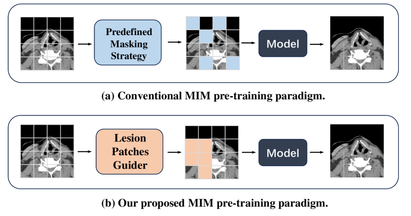
Fig. 1: Comparison between conventional MIM pre-trainingparadigm and our proposed HPM. (a) Conventional approaches can solve a given problem under predefined mask strategy. (b) Our proposed AMLP pre-training paradigm makes the model to guide the model to mask lesion patches to produce a chullenging pretext task.

In computer vision (CV), self-supervised learning methods heavily rely on contrastive learning (CL) approaches. Contrastive learning aims to extract representative information by minimizing the distance between similar pairs of images while maximizing the distance between dissimilar pairs of images. However, these methods often prioritize capturing global semantics in images and may sometimes sacrifice local details and non-object regions[8]. To address these challenges, researchers, inspired by masked language modeling (MLM) in natural language processing (NLP), have turned to masked image modeling (MIM) methods to explore potential solutions. Masked image modeling is designed to reconstruct masked regions within images, which typically contain information about important structures.

However, applying MIM methods used in natural images directly to medical images faces limitations. These is bacause there are notable differences between natural and medical images include: the small size and specific morphological features of lesions, which can lead models to unintentionally overlook critical regions, impacting downstream performance. Besides, the fixed high masking ratio used in conventional MIM methods can hinder effective capture of essential local information, emphasizing global details throughout encoding and decoding. This may cause critical local information, including the precise position and morphology of lesions, to be overlooked.

In this paper, to address these issues, we introduce a novel self-supervised medical image segmentation method, named Adaptive Masked Lesion Patch (AMLP). Compared to existing methods, AMLP incorporates four key improvement measures: Masked Patch Selection (MPS), Adaptive Masking Ratio (AMR) strategies, Attention Reconstruction Loss (ARL), and Category Consistency Loss (CCL).

To solve the problem that conventional MIM methods are not suitable for medical images, we propose MPS. MPS can learn lesion representatino learning by choosing the lesion patches to mask. Specifically, we input all patches into k-means clustering, classify them into foreground and background, and then rank them from large to small based on the probability of being classified as foreground to mask. This allows us to selectively prioritize masked image patches containing the lesion area, which can help learn more lesion representation information.

However, the unsupervised k-means clustering applied in MPS may have the problem of potential misclassification. we further calculate the Attention Reconstruction Loss (ARL) for each patch to ensure that the model accurately focuses on lesion patches during the training process. Additionally, we introduce the Category Consistency Loss (CCL), which helps the network distinguish differences between the reconstructed and original images in terms of categories, leading to a more accurate foreground-background distinction and enhancing the ability to learn lesion representation information.

Simultaneously, we propose the AMR strategy, which gradually increases the masking ratio and the final upper limit of the masking ratio, aiding the network in learning more global information in the initial encoding phases and raising the upper limit of learnable information, ultimately facilitating the acquisition of more representation information and improving overall performance.

The contributions can be summarized as follows:

• We identify the limitations under the applications of existing self-supervised learning methods based on Masked Image Modeling in the field of medical images, and propose a novel adaptive masking lesions patches benefits self-supervised medical image segmentation framework named AMLP.

• There exist four advancements in our proposed AMLP framework: First, we introduce a new Masked Patch Selection strategy (MPS), which enables the model to more accurately focus on lesion patches, through k-means clustering. Second, we introduce the Attention Reconstruction Loss (ARL) by calculating the relative attention reconstruction loss weight of each patch, ensuring that the network pays more attention to the difficult to reconstruct lesion patches. Furthermore, our proposed Category Consistency Loss (CCL) aids the network in distinguishing between the reconstructed image and the original image. This results in a more precise foreground-background distinction, optimizing clustering results and allowing the model to more accurately focus on the lesion area during the training process. Besides, we propose an Adaptive Masking Ratio Strategy (AMR) to progressively increase the masking ratio and the final upper limit of the masking rate to further enhance the model’s performance.

• Extensive experiments were conducted on two publicly available medical segmentation datasets. The results demonstrate that our method, with only 5% (or 10%) of labeled data, not only significantly outperforms state-of-the-art self-supervised baselines but also achieves comparable (sometimes even superior) performance to fully supervised segmentation methods with 50% (or 100%) of labeled data. This illustrates that our approach can achieve superior segmentation performance with minimal labeling efforts. Furthermore, ablation studies confirm the effectiveness and necessity of the four improvements (i.e., MPS, AMR, ARL, CCL) for AMLP to achieve its exceptional performance.

2 Related Work

2.1 Self-supervised learning

In recent years, self-supervised learning has garnered significant attention within the computer vision domain. Early self-supervised learning approaches primarily focused on learning feature representations through predicting various transformations applied to the same image, often relying on data augmentation techniques [6, 25, 7, 5, 26]. However, it’s worth noting that these methods tend to prioritize capturing global semantics within images, sometimes at the expense of local details and non-object regions [8]. A recent advancement in self-supervised learning, known as Masked Image Modeling, has brought a fresh perspective to pretraining in this field. The core principle of MIM revolves around learning representations by reconstructing occluded regions within images.

2.2 Contrastive learning

The objective of contrastive learning is to learn representations by drawing positive samples closer and pushing negative samples further away in the latent space, thereby distinguishing each image from others. This goal is typically achieved by applying a contrastive loss.

Currently, many contrastive learning methods have found successful applications in medical image segmentation. For instance, SimCLR [6] employs a contrastive loss function and multi-layer feature representation learning to facilitate self-learning on large-scale unlabeled data, thereby enhancing the model’s representational and generalization capabilities, but this method relies too much on data augmentation. To mitigate this issue, MoCo [13] further bolsters the model’s robustness and discriminative performance by introducing momentum contrastive learning and a nonlinear contrastive loss function, expanding the set of negative samples and enhancing sample variability, but it only focuses on sample-level information and ignores details. Subsequently, BYOL [11] promotes the learning of more discriminative and reconfigurable feature representations through bootstrapping methods and multi-task training, thus achieving significant performance improvements in self-supervised learning. And SwAV [5] proposes a method for unsupervised learning of visual features by contrastive cluster assignment. Effective feature learning and representation learning are achieved by comparing the similarity of samples in different cluster groupings.

However, these methods often emphasize acquiring global semantic features within images, potentially neglecting image details and non-subject regions [8]. Consequently, their performance in downstream segmentation tasks may be compromised.

2.3 Masked image modeling

Masked image reconstruction involves the process of masking specific image blocks within an image and then inputting them into a reconstruction network for the purpose of recovering the masked blocks. Various methods have been proposed in the field to address this task. Deepak et al.’s study [18] focuses on masking central regions of an image, with the reconstruction network using surrounding image data to infer the missing regions. MAE [12] utilizes an asymmetric encoder-decoder structure, dividing the image into equal-sized blocks and predicting the masked block based on the unmasked block of the image. In another approach, Maskfeat [22] introduces the Masked Feature Prediction method, enabling the model to predict masked features by randomly covering patches in the HOG feature map. This approach leads to self-supervised visual representation learning. SimMIM [23] extends the work of MAE by adjusting decoder weights and incorporating visible and masked patches as input, achieving results comparable to MAE while expediting the pre-training process. ConvMAE [10] enhances semantic information acquisition through MAE-based multi-scale encoding operations. BEiT v2 [19] takes a different approach by incorporating the discrete visual codebook generated by dVAE and introducing a pre-training stage for high-level semantic abstraction. BootMAE [9] introduces a supervised Bootstrapped Masked Autoencoder, using Masked Autoencoding objectives for prediction tasks on patch-level features of image blocks and introducing an additional supervised bootstrapping signal. In the context of medical images, FreMAE [21] addresses the challenge of distinguishing formal foreground from less useful background. It designs a skin rating system based on foreground pixels, enhancing task formulation efficiency and improving model learning performance.

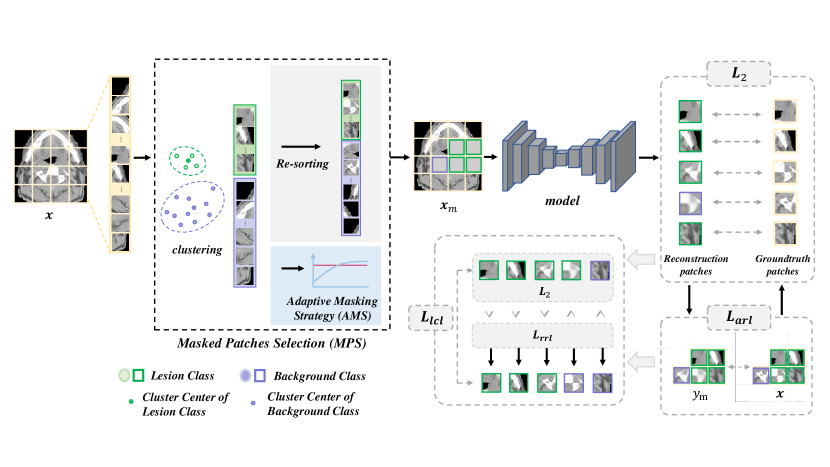
Fig. 2: The illustration of our proposed AMLP architecture. Green and purple areas represent lesion and background, respectively.

However, in the context of medical images, the methods currently used for selecting mask patches and determining mask ratios are considered unsatisfactory. These methods often rely on fixed or randomly determined mask positions and sizes. Furthermore, they have limitations when it comes to adapting to medical images, and applying techniques from the natural image domain directly to the medical field is challenging. This challenge arises from significant differences between medical images and natural images in several aspects.

One significant difference lies in the specific morphology and characteristics of lesions in medical images. These lesions are often small and have unique features, making them easily overlooked. Consequently, representations learned from such images often lack crucial information related to lesions, which subsequently hinders the performance of downstream tasks. Moreover, the use of a fixed high mask rate may make it difficult for the model to effectively capture critical local information, as it overly focuses on global information during both encoding and decoding phases. This leads to the neglect of important local details, such as the location and shape of lesions. This tendency can result in models failing to fully capture crucial local information in medical images, thereby limiting the learnable conditional mutual information and reducing the upper limit of expressive capacity ultimately achieved.

All masking models for these methods are mostly predefined [12, 23, 4, 19, 15, 14]. However, for medical images, we believe that learning to mask lesion parts is crucial, not only to guide the model in a more challenging way, but also to bring important priors to the input image, thereby improving the performance of various downstream tasks. Therefore, there is an urgent need to develop custom mask selection strategies and adaptive mask rate adjustment strategies for medical images to better accommodate their uniqueness.

3 Methodology

Fig. 2 provides an overview of our proposed AMLP, which comprises four key components. We commence by elucidating the masked patches selection strategy in Sec.3.1. Subsequently, the adaptive masking strategy is presented in Sec.3.4. Furthermore, Sec.3.2 details the attention reconstruction loss, while Sec. 3.3 introduces the category consistency loss, accompanied by the pseudocode delineating the complete process.

3.1 Masked patches selection strategy

Given that most current efforts in masked image modeling concentrate on natural images, with scant application in medical images, we propose a masked patches selection strategy tailored specifically for medical images. More specifically, the medical image $x$ is initially partitioned into $N$ equal-sized patches. Subsequently, each patch undergoes vectorization, and the resulting vectors are concatenated into a two-dimensional array. This array is then subjected to the k-means network for clustering. The cluster center point is set according to actual needs. In this paper, as only the segmentation of lesions is performed, the cluster center points are set as two categories: foreground (i.e., the image patch containing the lesion area) and background (i.e., the image patch that does not contain the lesion).

We divide all patches into two categories $x=\{x_{i},x_{\neg{i}}\}$ through k-means clustering. The group with the lesser number is the foreground $x_{i}$ and the large number is the background $x_{\neg{i}}$. They are assigned category labels of $1$ and $0$ respectively, $label_{x_{i}}=1$, $label_{x_{\neg{i}}}=0$. Then, according to the probability of being judged as the foreground (i.e., the distance from each patch to the center point of the foreground category), they are sorted from large to small, and a foreground-background ordered mask is performed according to the mask ratio.

To validate the effectiveness of the masked patches selection strategy, we conducted a proof from the perspective of the uncertainty of the sampling strategy. Specifically, a reduced uncertainty of $\{x_{i},x_{\neg{i}}\}$ indicates that the masked patches selection strategy can enhance the sampling strategy. We use entropy to measure the uncertainty of the joint probability distribution of samples $x_{i}$ and $x_{\neg{i}}$ under a given probability distribution $p(x_{i},x_{\neg{i}})$.

We denote the uncertainty of the sampling strategy as $H_{j}$, where $H_{1}$ represents the lower threshold of uncertainty,

$$H_{1}=\mathbb{E}_{p(x_{i},x_{\neg{i}})}\log P(x_{i},x_{\neg{i}}),$$ (1)

where $\mathbb{E}$ represents expectation, $P$ represents the probability, and $logP(x_{i},x_{\neg{i}})$ represents the logarithm of the joint probability of $x_{i}$ and $x_{\neg{i}}$, which is the probability that two or more events will occur simultaneously.

$H_{2}$ characterizes the uncertainty during the neural network learning process,

$$H_{2}=\mathbb{E}_{p}(x_{i},x_{\neg{i}})\log Q(x_{i},x_{\neg{i}}),$$ (2)

where $Q$ represents the neural network’s estimate of the joint probability distribution of samples $x_{i}$ and $x_{\neg{i}}$.

$H_{3}$ designates the optimal upper boundary of the Monte Carlo sampling strategy,

$$H_{3}=\mathbb{E}_{p}(\hat{x_{i}},\hat{x_{\neg{i}}})\log P(x_{i},x_{\neg{i}}),$$ (3)

where $\hat{x_{i}}$ and $\hat{x_{\neg{i}}}$ respectively represent the optimal foreground and background classification results.

The Monte Carlo sampling strategy is shown in the following formula. In the interval $[a,b]$, $f(x)$ represents the size of the value, $p(x)$ denotes the probability of occurrence, and the integral represents the total output value.

$$\int_{a}^{b}h(x)dx=\int_{a}^{b}f(x)p(x)dx=E_{p(x)}[f(x)].$$ (4)

As for $H_{1}$ and $H_{2}$, after training the neural network $Q$, we can obtain more accurate classification results of $x_{i}$ and $x_{\neg{i}}$. This means that the neural network’s estimate of the joint probability distribution of samples $x_{i}$ and $x_{\neg{i}}$ will change to be more accurate. Therefore, we can expect $H_{2}$, the uncertainty of the neural network’s estimate of the joint probability distribution of the samples, to decrease accordingly. This implies that by training neural networks, we can enhance sample classification accuracy, consequently diminishing uncertainty and refining sampling strategies. For $H_{3}$ and $H_{2}$, $H_{3}$ represents the optimal upper bound of the Monte Carlo sampling strategy, while $H_{2}$ is the uncertainty of the neural network’s estimate of the joint probability distribution of the sample. Because no matter how we improve the sampling strategy, the uncertainty of the neural network’s estimate of the joint probability distribution of the sample will not be less than the uncertainty of the optimal upper bound of the Monte Carlo sampling strategy, so we get $H_{3}\leq H_{2}$.

Consequently, we can get

$$H_{3}\leq H_{2}\leq H_{1}.$$ (5)

This implies that neural network training can enhance sample classification accuracy, resulting in reduced uncertainty and improved sampling strategies. As a result, this substantiates the effectiveness of the employed strategy for masked patch selection.

3.2 Attention reconstruction loss

However, the unsupervised k-means clustering applied in MPS may have the problem of potential misclassification. In order to reduce the impact of this problem, there is a need to assess the significance of individual patches within a collection and their likelihood of being classified as foreground. Therefore, we introduce an attention reconstruction loss. While the most direct approach involves comparing absolute reconstruction losses, such as the absolute reconstruction loss $L_{pred}$ calculated by feeding an image patch into the reconstruction network (e.g., using L2 loss as in MAE), it is insufficient when evaluating the importance of a single patch among all patches. Our primary objective is to identify image patches containing lesion areas within the image. Therefore, we must capture the relative relationships between patches. Additionally, as the scale of absolute reconstruction losses diminishes during training, relying solely on these values can overshadow the significance of relative differences among extracted patches. To address these concerns, we propose an attention reconstruction loss.

Specifically, we compute the attention reconstruction loss $L_{rrl}$ by calculating the ratio of the absolute reconstruction loss $L_{pred}$ for an individual patch to the average $L_{mean}$ of all reconstruction losses for masked image patches. This calculation is expressed as:

$$L_{rrl}^{i}=\frac{N\times L_{pred}^{i}}{\sum\limits_{i=1}^{N}(L_{pred}^{i})}.$$ (6)

Then we compare $L_{rrl}$ with $L_{mean}$. If $L_{rrl}\geq L_{mean}$, it indicates that the corresponding image patch holds relative importance among all masked patches. Additionally, in the absence of considering the k-means result, this image patch is likely to be classified as foreground and merits special attention. Conversely, if $L_{rrl}<L_{mean}$, the opposite holds true.

3.3 Category consistency loss

To enhance the network’s ability to distinguish between foreground and background patches, with a further specific focus on reconstructing lesion areas, we introduce a category consistency loss. This loss guides the periodic update of patch categories, combining insights from k-means clustering and the attention reconstruction loss. Specifically, following k-means clustering, each patch is assigned an original label $label_{ori}$, where foreground and background correspond to labels 1 and 0, respectively. Considering the limitations of unsupervised clustering, particularly during early training stages when significant misclassifications may occur, we refine these labels using the attention reconstruction loss.

We can update the category label for each patch based on the k-means clustering results and attention reconstruction loss. There are four possible cases:

(1) If the original category label $label_{ori}$ of the patch is $1$ and its attention reconstruction loss $L_{r}rl$ is greater than the average attention reconstruction loss $L_{mean}$ of all patches, which indicates $label_{ori}=1$ and $L_{rrl}>L_{mean}$, we set the new category label $label_{new}$ of this patch to be $1$.

(2) If the original category label $label_{ori}$ of the patch is $0$ and its attention reconstruction loss $L_{rrl}$ is less than the average attention reconstruction loss $L_{mean}$ of all patches, which indicates $label_{ori}=0$ and $L_{rrl}<L_{mean}$, we set the new category label $label_{new}$ of this patch to 0.

(3) If the original category label $label_{ori}$ of the patch is $1$ but its attention reconstruction loss $L_{rrl}$ is less than the average loss $L_{mean}$, which indicates $label_{ori}=1$ and $L_{rrl}<L_{mean}$, we randomly select a new category label $label_{new}$ in the list $[0,1]$ for this patch.

(4) If the original category label $label_{ori}$ of the patch is $0$ and its attention reconstruction loss $L_{rrl}$ is greater than the average loss $L_{mean}$, which indicates $label_{ori}=0$ and $L_{rrl}>L_{mean}$, we also randomly select a new category label $label_{new}$ in the list $[0,1]$ for this patch.

The reason for adopting this label update strategy is that we cannot quantify the impact of the k-means clustering results $label_{ori}$ and the attention loss weights $L_{rrl}$ during the initial training stage. However, we noticed that the k-means clustering results will gradually converge to the first two cases as the training progresses. Therefore, randomly selecting category labels can strike a good balance between their influences when the two indicate inconsistent results.

When $label_{new}\neq label_{ori}$, we calculate the category consistency loss using the following formula:

$$L_{lcl}=-\left[label_{new}\times\log(label_{ori}+\xi)\right.$$ (7)

$$\left.+(1-label_{new})\times\log(1-label_{ori}+\xi)\right].$$

This loss quantifies the disparity between the probability distribution predicted by the model and the actual label distribution, facilitating improved discrimination. $\xi=1e-10$ serves as a small positive value to prevent issues arising from $log(0)$.

Algorithm 1 AMLP

0:  $x$: input medical image

0:  $N$: number of patches

1:  Divide $x$ into $N$ patches: ${x_{1},x_{2},...,x_{N}}$

2:  Extract embeddings for patches and perform k-means clustering to create two classes: ${x_{i},x_{\neg i}}$

3:  Sort patches based on the probability of being foreground $x_{i}$

4:  Calculate the current masking ratio $\sigma$ using Eq. 6

5:  Determine the number of masked patches $n_{m}=\lfloor N\times\sigma\rfloor$

6:  Mask the top $n_{m}$ patches based on foreground and background probabilities, resulting in $x_{m}$

7:  for each training epoch do

8:     Reconstruct masked patches: ${y_{1},y_{2},...,y_{n_{m}}}$ from $x_{m}$

9:     for each patch $i$ do

10:        Compute attention reconstruction loss $L_{rrl}$ for patch $i$

11:     end for

12:     Update patch labels using attention reconstruction loss ($L_{rrl}$) and k-means results

13:     Calculate category consistency loss $L_{ccl}$

14:     Calculate the overall loss $L_{all}$ using Eq. 8

15:     Update model parameters by optimizing $L_{all}$

16:  end for

The final $L_{all}$ is the sum of the three losses.

$$L_{all}=L_{pred}+L_{rrl}+L_{lcl}.$$ (8)

3.4 Adaptive masking ratio strategy

In contrast to the commonly used high fixed masking ratio found in studies like MAE and SimMIM, we introduce a novel adaptive masking ratio strategy. This approach is based on the observation that MAE consistently employs a masking ratio of 75% throughout training. However, maintaining such a high masking ratio poses challenges for model learning, especially during the initial stages. While a higher masking ratio theoretically promotes the learning of more representations, a fixed 75% ratio may not be optimally effective. Is it possible to further increase the upper limit of the mask rate in some way, and further improve the performance by increasing the upper limit of the learnable representation ability?

To overcome this limitation, we introduce an innovative adaptive masking ratio strategy. In this approach, the masking rate gradually increases from the initial masking ratio as training rounds progress. The initial masking ratio, denoted as $\sigma_{0}$, is set at $25\%$, a value determined based on experimental findings in MAE.

Moreover, as the training progresses, the masking ratio dynamically adapts according to the equation:

$$\sigma=\sigma_{0}+\frac{\ln(x_{e})}{\tau},$$ (9)

where $x_{e}$ denotes the training epoch, and $\tau$ is a manually defined constant.

By integrating the masked patches selection strategy with the adaptive masking ratio strategy, we can compute the number of masked patches $n_{m}$ and the masked image $x_{m}$, where $n_{m}=\lfloor N\times\sigma\rfloor$. Subsequently, the masked image $x_{m}$ is fed into the reconstruction network to reconstruct the masked patches.

4 Experienments and Results

4.1 Datasets

To validate the effectiveness of our proposed AMLP framework, we conduct extensive evaluations on two publicly available medical image datasets, Hecktor [24, 1] and BraTS2018 [17, 2, 3].

Hecktor. The dataset comes from the MICCAI $2020$ challenge called HEad and the neCK TumOR Segmentation Challenge (Hecktor) for Head and Neck Tumor Segmentation. This dataset is a multimodal CT-PET dataset consisting of 201 3D scans. All CT volumes are limited to the range of $[-150,150]$ Hounsfield Units (HU).

Table 1: The results of AMLP and the state-of-the-art fully-supervised and self-supervised segmentation methods on the Hecktor and BraTS datasets with 5%, and 10% labeled data in terms of DSC and Sen.

3   Methods	Hecktor				BraTS
Modality		CT		PET		T1CE		T2		FLAIR		T1
Metrics		DSC$\uparrow$	Sen$\uparrow$	DSC$\uparrow$	Sen$\uparrow$	DSC$\uparrow$	Sen$\uparrow$	DSC$\uparrow$	Sen$\uparrow$	DSC$\uparrow$	Sen$\uparrow$	DSC$\uparrow$	Sen$\uparrow$
5%	Sup	0.1740	0.2337	0.5452	0.7044	0.3234	0.2703	0.3952	0.4371	0.4035	0.4837	0.1743	0.2702
	SimCLR	0.1733	0.2527	0.5720	0.7143	0.5403	0.5737	0.4310	0.5870	0.4342	0.5396	0.2908	0.4376
	BYOL	0.1967	0.2555	0.4487	0.5603	0.5245	0.4321	0.5245	0.5590	0.4561	0.6297	0.2811	0.4545
	SWAV	0.2307	0.4483	0.5517	0.7091	0.5252	0.4321	0.4160	0.5564	0.4346	0.6052	0.2277	0.4466
	MAE	0.2560	0.2966	0.5931	0.7301	0.5465	0.5276	0.4395	0.5134	0.4368	0.6108	0.2734	0.4596
	MaskFeat	0.2561	0.2894	0.5900	0.7277	0.5332	0.5173	0.4492	0.5012	0.4442	0.5937	0.2834	0.4542
	SimMIM	0.2413	0.2972	0.5892	0.7239	0.5421	0.5012	0.4289	0.4901	0.4525	0.6013	0.2801	0.4297
	ConvMAE	0.2611	0.3042	0.6042	0.7431	0.5552	0.5414	0.4497	0.5338	0.4247	0.6243	0.2979	0.4865
	BEIT V2	0.2759	0.3153	0.6133	0.7548	0.5508	0.5779	0.4504	0.5587	0.4501	0.6299	0.3027	0.4891
	BootMAE	0.2593	0.2978	0.5988	0.7345	0.5431	0.5358	0.4496	0.5134	0.4412	0.6164	0.2908	0.4739
	Ours	0.2905	0.3347	0.6296	0.7665	0.5762	0.5482	0.4721	0.5023	0.4693	0.6136	0.3297	0.5023
10%	Sup	0.2541	0.2703	0.5769	0.7067	0.4451	0.3696	0.4288	0.4716	0.4489	0.6225	0.2476	0.3366
	SimCLR	0.2951	0.3895	0.5779	0.7145	0.6024	0.6217	0.4846	0.5729	0.4720	0.5217	0.3551	0.4868
	BYOL	0.3088	0.393	0.5891	0.6990	0.5991	0.6323	0.4850	0.5710	0.4763	0.6329	0.3458	0.3535
	SWAV	0.2690	0.3340	0.5771	0.7004	0.5515	0.5646	0.4587	0.5794	0.4543	0.6084	0.2914	0.4694
	MAE	0.3195	0.4143	0.6058	0.7155	0.5881	0.5947	0.4765	0.5256	0.4587	0.6178	0.3578	0.4878
	MaskFeat	0.3078	0.4077	0.5955	0.7132	0.6065	0.5864	0.4613	0.5103	0.4625	0.6154	0.3351	0.4800
	SimMIM	0.2920	0.4025	0.5872	0.7221	0.5932	0.5701	0.4592	0.5082	0.4572	0.5921	0.3246	0.4725
	ConvMAE	0.3369	0.4273	0.6099	0.7183	0.6106	0.6208	0.5031	0.5667	0.4915	0.6246	0.3617	0.5123
	BEIT V2	0.3470	0.4388	0.6293	0.7217	0.6139	0.6315	0.5079	0.5897	0.4862	0.6446	0.3690	0.5334
	BootMAE	0.3225	0.4243	0.6221	0.7155	0.6203	0.6032	0.4857	0.5321	0.4751	0.6093	0.3624	0.5011
	Ours	0.3690	0.5004	0.6314	0.7331	0.6343	0.6023	0.5194	0.5482	0.4971	0.6324	0.3815	0.5782
Sup (50%)		0.3440	0.4331	0.6252	0.6582	0.5941	0.5324	0.5094	0.5328	0.4830	0.5664	0.4564	0.1358
Sup (100%)		0.3927	0.4736	0.6475	0.7307	0.7453	0.7204	0.5556	0.5575	0.5164	0.6561	0.4923	0.1582
3

Table 2: The results of AMLP and the state-of-the-art fully-supervised and self-supervised segmentation methods on the Hecktor and BraTS datasets with 5%, and 10% labeled data in terms of bIOU and HD95.

3   Methods	Hecktor				BraTS
Modality		CT		PET		T1CE		T2		FLAIR		T1
Metrics		bIOU$\uparrow$	HD95$\downarrow$	bIOU$\uparrow$	HD95$\downarrow$	bIOU$\uparrow$	HD95$\downarrow$	bIOU$\uparrow$	HD95$\downarrow$	bIOU$\uparrow$	HD95$\downarrow$	bIOU$\uparrow$	HD95$\downarrow$
5%	Sup	0.0690	62.7115	0.2493	69.0963	0.1487	55.0727	0.1330	47.4584	0.2055	33.2086	0.0484	59.5963
	SimCLR	0.0718	61.0090	0.2627	64.9785	0.1492	54.0091	0.1357	46.3305	0.2072	32.7433	0.0567	57.6039
	BYOL	0.0845	60.8153	0.2793	60.2143	0.1504	49.3725	0.1501	44.2871	0.2103	31.0754	0.0609	54.4291
	SWAV	0.0711	61.9957	0.2678	61.8257	0.1495	52.2436	0.1401	45.8792	0.2083	31.5867	0.0589	56.4368
	MAE	0.0999	58.7935	0.2802	54.9321	0.1472	48.2318	0.1489	43.1123	0.2106	30.2385	0.0842	53.5203
	MaskFeat	0.1067	59.0087	0.2799	58.9967	0.1505	49.0699	0.1463	43.7748	0.2117	32.7451	0.0775	54.2226
	SimMIM	0.0793	60.6234	0.2743	58.4102	0.1461	51.0855	0.1382	44.2219	0.2095	31.1998	0.0589	55.0105
	ConvMAE	0.1053	58.5928	0.2955	50.6654	0.1593	46.8451	0.1574	41.0145	0.2140	29.1014	0.1063	51.1002
	BEIT V2	0.1374	57.4124	0.2994	48.2849	0.1607	46.3542	0.1623	40.3721	0.2152	28.5621	0.1112	50.2631
	BootMAE	0.1201	59.5928	0.2836	52.7976	0.1512	47.1273	0.1537	41.2457	0.2128	29.8902	0.0928	52.4317
	Ours	0.1514	57.2823	0.3113	40.5376	0.1723	44.2326	0.1750	40.6362	0.2156	28.2352	0.1157	50.2342
10%	Sup	0.1224	64.0604	0.3199	41.8627	0.1643	50.9107	0.1510	43.9483	0.1724	30.4918	0.1042	52.8203
	SimCLR	0.1504	46.3870	0.3581	66.4539	0.2758	37.6094	0.2020	38.0898	0.2203	28.5869	0.1247	46.2637
	BYOL	0.1501	58.9947	0.3397	55.0181	0.2901	36.1710	0.1820	42.4852	0.2075	27.9066	0.1201	39.8026
	SWAV	0.1543	59.5009	0.3573	50.8417	0.2287	46.0846	0.1889	44.0658	0.2036	38.6023	0.1035	61.8490
	MAE	0.1702	55.2376	0.3445	46.1427	0.3113	32.7709	0.2167	32.9846	0.2145	26.9349	0.1182	35.9123
	MaskFeat	0.1634	57.2447	0.3618	47.6183	0.3024	33.2451	0.1987	35.6779	0.2109	27.3426	0.1245	37.5428
	SimMIM	0.1601	58.3412	0.3511	48.8915	0.2975	34.8762	0.2063	37.5124	0.2096	29.8875	0.1223	39.3501
	ConvMAE	0.1882	50.3523	0.3739	41.7655	0.3421	25.9865	0.2301	28.0147	0.2012	25.6731	0.1356	27.8754
	BEIT V2	0.1990	48.7192	0.3899	39.8887	0.3578	22.4567	0.2253	23.8829	0.2218	24.2587	0.1428	24.7159
	BootMAE	0.1788	54.5214	0.3612	42.9639	0.3182	27.9943	0.2173	30.5402	0.2186	25.9823	0.1324	33.7837
	Ours	0.2368	44.2361	0.4032	35.3453	0.3745	20.3453	0.2253	23.2375	0.2234	25.1484	0.1402	23.5632
Sup (50%)		0.1882	46.3327	0.3713	36.0685	0.3557	23.8802	0.2030	23.6540	0.2354	24.7391	0.1358	22.6528
Sup (100%)		0.2398	50.0361	0.3928	34.7032	0.3962	18.8440	0.2238	19.7038	0.2477	22.0652	0.1582	20.8641
3

BraTS2018. This dataset was released by the BraTS’18 challenge hosted by MICCAI 2018 for brain tumor segmentation. It contains high-grade glioma (HGG) data and low-grade glioma (LGG) data, where only $210$ 3D MRI HGG data are used in our experiments. Furthermore, this dataset contains four modalities: T1, T1CE, T2 and FLAIR. In the self-supervised pre-training stage, all slices containing the corresponding organ are kept (i.e., only completely black images are discarded); in the downstream stage, objects (i.e. tumors in our work) are segmented through fully supervised fine-tuning , so only slices containing the object of interest (i.e. tumor) and corresponding labels are kept.

4.2 Baselines

In our evaluation of the proposed AMLP, we consider two primary categories of baselines: fully supervised learning and self-supervised learning. These baselines serve as essential points of comparison to assess the effectiveness of AMLP.

For fully supervised learning, we employ randomly initialized U-Net architecture without self-supervised pretraining. This approach involves training the model from scratch, with annotations provided at different levels of granularity, specifically 5% and 10% annotations. The selection of ”Fully Supervised” as a baseline allows us to gauge the impact of self-supervised pretraining on model performance.

In the realm of self-supervised learning, we consider two subcategories: contrastive learning and mask image modeling. In the category of contrastive learning, we choose the SimCLR, BYOL, SwAV methods as baselines. The selection of these methods as baselines is based on their established effectiveness in capturing informative representations. For mask image modeling, we explore several state-of-the-art methods as baselines, including MAE, Maskfeat, SimMIM, ConvMAE, BEiT v2, and BootMAE. These methods are chosen because of their capacity to model complex relationships within medical images by utilizing mask-based objectives.

We evaluate the quality of the learned representations by transferring them from different self-supervised learning methods to downstream segmentation tasks. Unlike linear probing, we perform end-to-end fine-tuning to assess the pre-trained model’s effectiveness. Additionally, we include results from fully supervised learning with larger annotation ratios, specifically 50% and 100%, for a more holistic comparison of the proposed AMLP against conventional training approaches. This structured approach to baselines ensures a systematic evaluation of AMLP in comparison to a diverse set of benchmarks, covering both fully supervised and self-supervised paradigms.

4.3 Pre-processing

We apply the following pre-processing steps: (i) re-sampling of all volumes and corresponding labels to a fixed pixel size $1.0\times 1.0\times 1.0$ $mm^{3}$ using nearest-neighbour interpolation, intensity normalization of each 3D volume, clip the value into the range $[1$, $99]$ and normalize the image with mean and std for region nonzero. (ii) all 2D images and corresponding 2D labels are obtained from the z-axis of 3D volumes. The dimension $d$ for each dataset are: (a) Hecktor: $d$ = $144\times 144$, and (b) BraTS2018: $d$ = $160\times 160$.

4.4 Implementation details

Our AMLP is implemented based on Torch 1.6.0 and CUDA-10.1. All experiments are done on $8$ GeForce RTX 2080 GPUs. For self-supervised learning, the AdamW [16] optimizer is used, with a learning rate of $1e-4$. The temperature parameter $t$ is set to $0.1$. The batch size is $48$ for Hecktor and $36$ for BraTS2018. And a total of $800$ epochs is trained, and the number of divided patches is 256.

For transfer learning, the U-Net [20] for downstream segmentation tasks is also trained with the AdamW optimizer. The initial learning rate is $1e-4$, the weight decay is $0.0001$, and the learning rate strategy is cosine decay. When using $5\%$ labels, the batch size is set to $31$ for Hecktor and $56$ for BraTS2018. When using $10\%$ labels, the batch size is set to $90$ for Hecktor and $70$ for BraTS2018. To make the network reach convergence, $70$ epochs are trained for Hecktor and BraTS2018.

Besides, all baselines are implemented and run using similar procedures and settings as those in their original papers, where all self-supervised methods are learned in a two-stage learning way, i.e., first pre-trained using only unlabeled data and then fine-tuned using solely labeled data and additional parameter adjustments are made to our best efforts.

4.5 Network architecture

We use the U-Net, which includes four downsampling and upsampling modules, as a segmentation backbone network for all methods. Each downsampling module consists of two $3\times 3$ convolutions and a $2\times 2$ max pooling with stride $2$, while each upsampling module consists of two $3\times 3$ convolutions and a $2\times 2$ transposed convolution with stride $2$. This U-Net network also serves as the backbone network of BASE and AMLP.

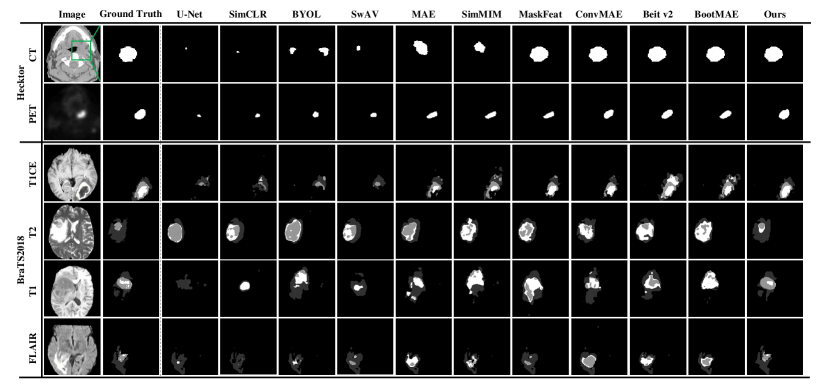
Fig. 3: Visualized segmentation results on the Hecktor and BraTS2018 datasets with $10\%$ labeled data. The first two rows are the results of the Hecktor dataset, where the head and neck tumor (only one type of tumor) is marked with white in the segmentation results. The last four rows are the results of the BraTS2018 dataset, where WT (whole tumor), ET (enhancing tumor), and TC (tumor core) are marked with light gray, medium gray and white, respectively, in segmentation results.

4.6 Evaluation metrics

We employ four widely used metrics to evaluate all methods, including Dice Similarity Coefficient (DSC), Sensitivity (Sen), Mean Intersection of Union Boundaries (bIOU), and 95% Hausdorff Distance (HD95). DSC and Sen are indicators of AMLP; bIOU and HD95 are measures of distance. DSC is used to measure the similarity between predictions and ground truth. Sen represents the percentage of correct segmentations among the true segmentations. Boundary IoU (BIoU) is a widely used boundary-based metric. Hausdorff distance (HD) is a widely used distance-based metric, here we use HD95 (a variant of HD) to remove the effect of a very small subset of outliers. Among them, except for HD95, the higher the value of these indicators, the better the performance. All evaluation metrics were calculated using 3D scans of each patient and then averaged as the final result. The specific formula is defined as follows:

$$DSC=\frac{2\times TP+\epsilon}{T+P+\epsilon},$$ (10)

$$SEN=\frac{TP+\epsilon}{TP+FN+\epsilon},$$ (11)

$$bIOU=\frac{(G_{d}\cap G)\cap(P_{d}\cap P)}{(G_{d}\cap G)\cup(P_{d}\cap P)},$$ (12)

$$HD95=max_{k95\%}[d(P,G),d(G,P)],$$ (13)

where TP, FP, and FN are the number of true positive points, false positive points, and false negative points, respectively. T is the number of ground-truth points of this class, $P$ is the number of predicted punctual points, $G$ is the number of ground-truth punctual points, $P_{d}$ is the number of predicted boundary punctual points, $G_{d}$ is the number of ground-truth true positive boundary points, $d(*)$ is a function to calculate the surface distance. Finally, $\epsilon$ is a small constant to avoid division by zero, it is set to $1e-4$ in our experiments.

4.7 Main results

To investigate the effectiveness of AMLP, we conduct experiments on two datasets and compare its performance with two state-of-the-art baselines: Fully Supervised Baseline (i.e., Fully Supervised) and Self-Supervised Baselines (i.e., SimCLR, BYOL, SwAV, MAE, Maskfeat, SimMIM, ConvMAE, BEIT V2, BootMAE). For a fair comparison, we use the same backbone network (U-Net) with 5% and 10% annotations across all methods. The experimental results are shown in Table 4.1 and Table 4.1. Table 4.1 and Table 4.1 respectively refer to two types of indicators: similarity metrics (i.e., DSC, Sen) and distance metrics (i.e., bIOU, HD95). The visualization of the segmentation results of AMLP and the self-supervised baselines on the Hecktor and BraTS2018 databases is shown in Fig. 3.

As shown in Table 4.1 and Table 4.1, AMLP generally outperforms all the state-of-the-art self-supervised medical image segmentation baselines in terms of all evaluation metrics and two small label-ratio settings (i.e., 5% and 10%) on both datasets, and its performances are similar to (and sometimes even better than) the fully supervised solution using much higher ratios (i.e., 50% and 100%) of label data. This observation proves that the proposed AMLP can achieve superior medical image segmentation performances using only a small number of annotations, which thus greatly reduces the labeling workload of applying intelligent medical image segmentation systems in clinical practices. The detailed analysis is as follows.

4.7.1 Comparison with state-of-the-art fully-supervised methods

As shown in Table 4.1 and Table 4.1, self-supervised learning methods (including the proposed AMLP) achieve much better segmentation performances than the fully supervised baseline with the same ratio of labeled data in also cases on both datasets. This is because besides of the small amount of labeled data, self-supervised methods can mine additional useful information from the large amount of unlabeled data.

Furthermore, AMLP generally outperforms the baseline model that is fully supervised learning from scratch by a large margin with $5\%$ and $10\%$ annotations. The performance of AMLP with $5\%$ annotations can be close to or even better than that of the fully supervised method with $50\%$ annotations. As for $10\%$ annotations, AMLP not only outperforms the fully supervised method with $50\%$ annotations but also outperforms the fully supervised method with $100\%$ annotations in the PET modality on Hecktor. Specifically, in the case of 5% annotation, we first find that AMLP is 11.65%, 10.1%, and 8.24% higher than the fully supervised method with 5% annotations on the CT modality of the Hecktor dataset, for DSC, Sen, and BIoU, respectively, and HD95 is 4.4292 lower than U-Net; while on the T1 modality of the Brats2018 dataset, DSC, Sen, and BIoU are 15.54%, 23.21%, and 6.73% higher than the fully supervised method with 5% annotations, respectively, and HD95 is 9.3621 lower than U-Net. And similarly, in the case of 10% annotation, AMLP is 11.49%, 23.01%, and 11.44% higher than the fully supervised method with 10% annotations on CT modality of the Hecktor dataset for DSC, Sen, and BIoU, respectively, and HD95 is 19.8243 lower; while on the T1 modality of the Brats2018 dataset, DSC, Sen, and BIoU are 13.39%, 24.16%, and 3.6% higher than the fully supervised method with 10% annotations, respectively, and HD95 is 29.2571 lower. This is because the ability of our method to learn more valuable representations from a large amount of unlabeled data, thereby improving the performance of downstream segmentation models.

4.7.2 Comparison with state-of-the-art self-supervised methods

Then, we further compare our AMLP with the state-of-the-art self-supervised methods.We can see that our AMLP also significantly outperforms these methods in almost all cases on both datasets. Consequently, This proves our argument that AMLP is capable to learn more comprehensive and fruitful information and features from the unlabeled multimodal data than the SOTA self-supervised contrastive learning baselines, and thus achieves better medical image segmentation performances.

Specifically, in the case of 5% annotation, we proposed AMLP is 1.46%, 1.94%, and 1.4% higher than the second-best result at 5% annotation ratio on the CT modality of the Hecktor dataset for DSC, Sen, and BIoU, respectively; while at 5% annotation ratio on the T1 modality of the Brats2018 dataset, DSC, Sen, and BIoU are 2.7%, 1.32%, and 0.45% higher than the second best result, respectively, and HD95 is 0.0289 lower. In the case of 10% annotation, AMLP is 2.2%, 6.16%, and 3.78% higher than the second-best result at 10% annotation ratio on the CT modality of the Hecktor dataset for DSC, Sen, and BIoU, respectively, and HD95 is 4.4831 lower; while at 10% annotation ratio on the T1 modality of the Brats2018 dataset, DSC, and Sen are 1.25%, and 4.48% higher than the second best result, respectively, and HD95 is 1.1527 lower. The superior performance of AMLP can be attributed to the fact that it determines more appropriate and challenging adaptive masks for each image. By reducing the uncertainty of the masked patches and increasing the upper limit of conditional mutual information, allowing for the learning of more comprehensive and effective representation information.

In addition, we have observed that few of our method’s results may not always the best in some scenarios. This can be attributed to the challenge of fully capturing all informative representations from the limited labeled data during self-supervised pretraining. To further boost performance, future work could investigate incorporating external knowledge or multi-task learning to better direct self-supervised feature learning towards more segmentation-relevant representations. By improving the model’s ability to extract informative cues tailored for the end task during pretraining, we can potentially close the remaining performance gap even with limited annotation.

Table 3: Results of our ablation studies on the Hecktor and BraTS2018 datasets with 5% and 10% labelled data.

Ratios	Methods	Hecktor				BraTS2018
		CT		PET		T1CE		T2		FLAIR		T1
		DSC	HD95	DSC	HD95	DSC	HD95	DSC	DH95	DSC	HD95	HD95	HD95
5%	Fully Supervised	0.1740	62.7115	0.5452	69.0963	0.3234	55.0727	0.3952	47.4584	0.4035	33.2086	0.1743	59.5963
	BASE	0.2373	61.2351	0.5692	62.3420	0.5307	53.7239	0.4152	45.2062	0.4401	32.6258	0.2486	57.7398
	MPS	0.2679	60.0462	0.5921	58.6432	0.5501	51.3462	0.4396	43.6237	0.4581	30.9462	0.2791	55.0862
	AMR	0.2512	61.2337	0.5834	60.7285	0.5425	52.6132	0.4285	44.9625	0.4423	31.4195	0.2673	56.6478
	CRCL	0.2481	60.7930	0.5802	61.1427	0.5399	52.0410	0.4205	44.8291	0.4471	30.4632	0.2578	56.9203
	MPS-AMR	0.2831	58.6127	0.6244	43.4581	0.5752	45.4307	0.4693	40.4502	0.4687	28.4192	0.3143	50.9173
	MPS-CRCL	0.2804	59.3581	0.6114	51.2614	0.5637	48.7651	0.4563	41.5846	0.4649	29.6834	0.3062	52.3516
	AMR-CRCL	0.2816	60.0574	0.6044	55.8031	0.5580	50.0917	0.4409	42.9724	0.4600	30.1734	0.2916	53.4329
	AMLP(Ours)	0.2905	57.2823	0.6296	40.5376	0.5762	44.2326	0.4721	40.6362	0.4693	28.2352	0.3297	50.2342
10%	Fully Supervised	0.2541	64.0604	0.5769	41.8627	0.4451	50.9107	0.4288	43.9483	0.4489	30.4918	0.2476	52.8203
	BASE	0.3006	58.2945	0.5932	49.6235	0.5892	47.6230	0.4518	40.4253	0.4599	29.0526	0.3351	45.2526
	MPS	0.3318	55.4185	0.6079	47.2145	0.6067	32.4192	0.4827	31.2364	0.4823	27.2345	0.3576	35.4273
	AMR	0.3187	57.6234	0.5958	48.5263	0.5903	41.5234	0.4735	38.6234	0.4748	28.9632	0.3469	39.9634
	CRCL	0.3105	57.7369	0.5960	49.1352	0.5883	45.8265	0.4693	39.6515	0.4701	28.5238	0.3390	41.3282
	MPS-AMR	0.3671	46.5192	0.6303	37.4192	0.6332	22.3254	0.5157	24.2163	0.4967	25.4163	0.3807	24.2154
	MPS-CRCL	0.3532	50.2356	0.6221	39.7684	0.6256	26.5163	0.5012	27.3175	0.4912	26.4192	0.3732	29.6234
	AMR-CRCL	0.3481	51.3252	0.6185	42.4560	0.6185	30.5124	0.4976	30.2864	0.4891	27.4258	0.3701	30.5128
	AMLP(Ours)	0.3690	44.2361	0.6314	35.3453	0.6343	20.3453	0.5194	23.2375	0.4971	25.1484	0.3815	23.5632

4.7.3 Analysis of visualized segmentation results

Moreover, all the above findings are also well supported by the visualized results in Fig. 3, where AMLP achieves obviously better (i.e., more similar to the ground-truth) segmentation results than all the self-supervised medical image segmentation methods. Several key observations can be made by comparing AMLP against other self-supervised methods:

Firstly, contrastive learning approaches like SimCLR, BYOL and SvAW exhibit poor adherence to the ground truth, with prevalent over-segmentation and inaccurate lesion contours. This indicates their limited capacity for precise localization and detail retention. Secondly, reconstruction-based methods like MAE, MaskFeat and SimMIM exhibit finer segmentation details and improved edge alignment over contrastive counterparts. This results from their mask reconstruction objectives that compel focus on local regions. However, they still display limitations in lesion boundary delineation, with occasional blurring or discontinuities. This suggests room for improvement in capturing subtle morphological characteristics. Finally, AMLP produces segmentation outputs most closely resembling the ground truth. Lesion contours are cleanly delineated with smooth edges. Fine details within lesions are also well retained. This illustrates AMLP’s strength at capturing subtle cues and contexts vital for medical image segmentation.

In summary, the visualized examples clearly highlight AMLP’s advantages over existing self-supervised medical segmentation techniques. By selectively focusing on informative regions and optimizing learned representations, AMLP generates accurate and detailed segmentation maps from limited annotation. The qualitative results further validate its effectiveness for this task.

4.8 Ablation studies

Since there are four improvements, i.e., masked patches selection strategy, adaptive masking ratio strategy, attention reconstruction loss, and category consistency loss, ablation studies are conducted to verify the effectiveness of these advanced components. Specifically, we have implemented several intermediate models for self-supervised pre-training: (i) BASE: BASE is a method that leverages the U-Net network architecture for self-supervised pretraining. It differs by broadening its objectives, incorporating self-supervised learning to acquire feature representations from masked image patches with l2 loss. Additionally, BASE shifts its training approach to embrace self-supervised learning, allowing training on unlabeled data. (ii) MPS: MPS incorporates only the masked patches selection strategy on top of BASE. This allows us to evaluate the isolated impact of focusing masking on lesion-containing patches; (iii) AMR: AMR incorporates only the adaptive masking ratio strategy on top of BASE. This enables assessment of progressively increasing the masking ratio during training; (iv) CRCL: CRCL combines the attention reconstruction loss and category consistency loss on top of BASE. This examines the joint effect of the two losses in enhancing model learning; (v) MPS-AMR: MPS-AMR integrates both the masked patches selection strategy and adaptive masking ratio strategy on top of BASE. This explores the combined influence of selective masking and adaptive ratio adjustment; (vi) MPS-CRCL: MPS-CRCL integrates the masked patches selection strategy with the joint losses (CRCL) on top of BASE. This evaluates the synergy between selective masking and enhanced objective modeling; (vii) AMR-CRCL: AMR-CRCL incorporates the adaptive masking ratio strategy together with the combined losses (CRCL) on top of BASE. This analyzes the combined effects of adaptive ratio with enhanced objectives; (viii) AMLP (Ours): AMLP represents the full model incorporating all improvements on top of BASE. . The ablation studies are conducted on Hecktor and BraTS2018 datasets using 5% and 10% ratios of annotations, and the corresponding results are shown in Table 4.1 and Table 4.1. On the other hand, to study the effectiveness of different losses in our method, we also conduct loss ablation experiments on two datasets with 5% labeled data as shown in Table 5.

4.8.1 Effectiveness of MPS

Ablation studies demonstrate the MPS module’s effectiveness in improving model performance on both datasets. As an illustration, employing only MPS in the Hecktor CT modality with 5% labeled data yielded a notable 0.0306 increase in the DSC and a reduction of 1.4764 in the HD95. This enhancement can be attributed to the MPS module’s capacity to enhance precise representation learning by selectively masking regions that contain lesions. Lesions, with their intricate shapes and blurred boundaries, present a more formidable reconstruction challenge in contrast to simpler background regions. By prompting the model to infer these intricate masked areas, MPS delivers a tailored supervised signal for acquiring valuable lesion representations. In conclusion, these improvements substantiate the effectiveness of MPS in facilitating focused lesion representation learning via tailored masking of the most informative signals.

Table 4: Results of different masking strategies ablation studies on the Hecktor and BraTS2018 datasets with $10\%$ labeled data.

Losses	Hecktor				BraTS2018
	CT		PET		T1CE		T2		FLAIR		T1
	DSC	DH95	DSC	DH95	DSC	DH95	DSC	DH95	DSC	DH95	DSC	DH95
random	0.3256	50.2351	0.6156	45.2365	0.6038	30.2532	0.4957	30.3209	0.4624	28.2390	0.3425	35.2624
hard to easy	0.3487	47.2630	0.6202	40.9863	0.6195	25.2263	0.5072	27.0117	0.4782	26.8805	0.3752	28.8764
easy to hard (Ours)	0.3690	44.2361	0.6314	35.3453	0.6343	20.3453	0.5194	23.2375	0.4971	25.1484	0.3815	23.5632

4.8.2 Effectiveness of AMR

Ablation experiments provide convincing evidence of the AMR module’s effectiveness in enhancing model performance. As an illustration, integrating AMR alone on the BraTS2018 T1 modality with 5% labeled data led to a noteworthy 1.87% increase in DSC and a sizable 1.092 reduction in the HD95. This boost stems from AMR’s unique adaptive masking schedule, which promotes continuous representation learning. Commencing training with a low masking ratio facilitates initial global representation learning. Subsequently, gradually elevating the masking ratio progressively intensifies task difficulty. By incrementally masking larger regions, the model is compelled to expand its comprehension of visual contexts and relationships to reconstruct missing areas. Ultimately, this dynamic schedule allows the learning of richer and more varied representations compared to static masking ratios. Through tailored adjustment of masking difficulty, AMR enables the model to steadily augment its representational capacity over time. The gains validate that AMR’s adaptive regimen provides impactful supervised signals tailored to comprehensive feature learning.

Table 5: Results of loss-based ablation studies on the Hecktor and BraTS2018 datasets with $5\%$ labeled data.

Losses	Hecktor				BraTS2018
	CT		PET		T1CE		T2		FLAIR		T1
	DSC	DH95	DSC	DH95	DSC	DH95	DSC	DH95	DSC	DH95	DSC	DH95
$L_{l2}$	0.2373	61.2351	0.5692	62.3420	0.5307	53.7239	0.4152	45.2062	0.4401	32.6258	0.2486	57.7398
$L_{l2}+L_{rcl}$	0.2863	59.2341	0.6152	49.2341	0.5752	47.1562	0.4673	42.1345	0.4617	29.9632	0.3187	53.2635
$L_{l2}+L_{ccl}$	0.2592	60.4562	0.5745	55.4562	0.5343	53.5263	0.4231	44.5263	0.4462	32.3526	0.2614	56.8561
$L_{l2}+L_{rcl}+L_{ccl}$ (Ours)	0.2905	58.2823	0.6296	40.5376	0.5762	44.2326	0.4721	40.2362	0.4693	28.2352	0.3297	50.2342

4.8.3 Effectiveness of CRCL

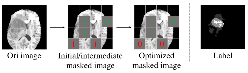
Fig. 4: Visualization process of CRCL progress. Among them, 1 represents the lesion category, and 0 represents the background category.

To evaluate the effectiveness of the combined losses, we conducted loss-based ablation studies on Hecktor and BraTS2018 datasets with 5% and 10% labeled data. The combined losses refer to the attention reconstruction loss $L_{rcl}$ and category consistency loss $L_{ccl}$. Since $L_{ccl}$ depends on the output of MPS, it is excluded when evaluating the part that does not contain MPS.

The results are shown in Table 5 and Fig. 4. The ablation results demonstrate that incorporating the attention reconstruction loss $L_{rcl}$ alone can enhance model performance. For instance, on the CT modality of the Hecktor dataset with 5% labeled data, adding CRCL improves the DSC by 1.08% and a sizable 0.4421 reduction in the HD95. This validates that $L_{rcl}$ assists the model in focusing more precisely on lesion areas during training. The combination of both $L_{rcl}$ and $L_{ccl}$ can further boost performance, as evidenced in MPS-CRCL results. By continually concentrating learning on lesion regions, CRCL enables the acquisition of superior feature representations. Besides, the visualization shown in Fig. 4 shows that CRCL can effectively correct misclassification issues.

4.8.4 Effectiveness of masking strategies

Furthermore, we designed additional ablation study on validating the necessity of masking lesion patches and masking background. The results are shown in Table 4 Specifically, three masking strategies were compared: (i) Random masking: randomly mask image patches. (ii) Hard to easy: first mask lesion patches, then gradually increase masked background patches. (iii) Easy to hard: first mask background patches, then gradually increase masked lesion patches until fully masked.

The results demonstrate that the ”hard to easy” strategy significantly outperforms the other two, indicating that masking lesion areas leads to better performance than masking background. The underlying reason is that lesion regions have irregular morphology and blurred boundaries, imposing greater difficulty for reconstruction and forcing the model to specialize in learning these critical areas. This enables the acquisition of richer feature representations. In contrast, masking only background regions first fails to provide effective representation learning.

4.9 Additional experiments

Table 6: Results of different clustering methods on Brats2018 with 10% labeled data.

methods	k-means	hierarchical	t-SNE	DBSCAN
DSC	0.3633	0.3474	0.3716	0.3592
complexity	$O(n)$	$O(n^{2})$	$O(n^{2})$	$O(n^{2})$

To determine the optimal clustering approach for lesion segmentation, we evaluated four prevalent unsupervised methods: k-means, hierarchical clustering, t-SNE and DBSCAN. As summarized in Table 6, k-means achieved a Dice score of 0.3633 on the Brats2018 dataset with 10% labeled data. This result was only 0.83% lower than the best score of 0.3716 attained by t-SNE. However, k-means held a significant advantage in computational complexity, with a time complexity of $O(n)$ compared to $O(n^{2})$ for other methods. The combination of strong performance approaching the optimum score with low complexity highlights k-means as an efficient and effective choice compatible with the hardware and time constraints of real-world clinical deployment. Compared to hierarchical and density-based clustering, k-means provides a favorable trade-off between accuracy and efficiency critical for practical utility.

5 Discussion and future work

5.1 Social impact for proposed algorithm

The proposed model can be widely used in a lot of clinical scenarios, where the work of segmenting medical images is needed to effectively reduce the workload of doctors and improve the efficiency and accuracy of medical image segmentation. We take radiotherapy for cancer as an example, where doctors need to accurately delineate the outline of the tumor area on the patient’s 3D CT or PET images as the radiotherapy target area. However, each 3D CT and PET is composed of hundreds of slices, and will take an experienced doctor several hours to annotate them one by one. Moreover, since the edge of the tumor is uneven and very difficult to delineate, to ensure the accuracy and comprehensiveness of labeling, it is usually necessary for multiple doctors to label the same image independently, and then gather them together as the final results. Consequently, the whole image segmentation process is very time-consuming and laborious; this not only greatly consumes the medical social resources (e.g., the time of experienced doctors), but may also bring long waiting times for the patient and delay the treatment. By applying our proposed automatic segmentation solution in such clinical practices, the model can generate the draft segmentation results automatically in seconds, which can then be sent to experienced doctors for fine-tuning. This thus greatly reduces the workload of doctors and saves both time and money for patients.

More importantly, different from the fully-supervised segmentation solutions that require a huge number of annotated data for training, our self-supervised segmentation solution can achieve accurate segmentation using only a small amount of labeled training data. This thus greatly reduces the application requirements and enhances the deployment efficiency of automatic medical image segmentation systems in clinical practices. Consequently, this further enhances the segmentation model’s usability and reduces the time and examination costs of patients in some clinical scenarios.

5.2 Limitations and future work

Due to the distinct characteristics of medical images compared to natural images, directly applying existing self-supervised methods with generic masking strategies may lead to unsatisfactory results on medical datasets. The current lesion area masking strategy in our method still has some room for improvement. For instance, we can significantly improve the mask selection strategy by integrating domain-specific expertise and prior knowledge from the field of medicine. This could involve considering prevalent lesion locations associated with various diseases and accounting for the distinct morphological characteristics exhibited by different types of lesions. Employing such tailored mask selection techniques holds substantial promise in enhancing the model’s ability to discern between various diseases and lesions, thus contributing to the overall improvement of medical image segmentation.

While our method demonstrates superior performance in comparison to existing self-supervised solutions, there remains a little performance gap when confronted with a limited portion of labeled data, especially when compared to fully supervised methods. The task of closing this gap stands as an open research challenge but can potentially be addressed through the incorporation of more advanced techniques. One avenue of exploration is the application of reinforcement learning for both mask selection and reconstruction. Specifically, the mask selection process can be conceptualized as a Markov decision process, allowing for dynamic optimization through policy gradient methods, potentially surpassing the efficacy of our current masking strategy.

In summary, combining cross-disciplinary knowledge with deep learning methods stands as a key direction for future medical image segmentation research. Such integrated approaches have potential to enhance model performance, meeting the demands for high-quality segmentation in healthcare, providing more reliable support for patient health, and playing a vital role in complex medical scenarios.

6 Conclusion

In this paper, we proposed a self-supervised framework named Adaptive Masked Lesion Patches (AMLP) for medical image segmentation. This architecture can leverage unlabeled medical images for representation learning by masking and reconstructing lesion patches. Specifically, under the guidance of the masked patch selection strategy, the model can focus on learning informative representations of important lesion areas. In addition, we designed an attention reconstruction loss and category consistency loss. These losses strengthen the model’s focus on hard-to-reconstruct patches likely depicting lesions, while enhancing distinction between lesions and background. Moreover, we developed an adaptive masking ratio strategy that gradually increases the masking ratio over training to expand the scope of reconstructible information. Through extensive experiments on multiple public datasets, we demonstrate that using only a small portion of annotations, our method can achieve comparable or even superior segmentation performance to fully supervised methods trained on much larger labeled datasets. This significantly increases the utilization of abundant unlabeled medical images, while reducing annotation requirements. The learned representations can also be effectively transferred to various downstream medical segmentation tasks.

Acknowledgments

This work was supported by the National Natural Science Foundation of China under the grants 62276089, 61906063 and 62102265, by the Natural Science Foundation of Hebei Province, China, under the grant F2021202064, by the “100 Talents Plan” of Hebei Province, China, under the grant E2019050017, by the Open Research Fund from Guangdong Laboratory of Artificial Intelligence and Digital Economy (SZ) under the grant GML-KF-22-29, and by the Natural Science Foundation of Guangdong Province of China under the grant 2022A1515011474.

References

- Andrearczyk et al. [2020] Andrearczyk, V., Oreiller, V., Vallières, M., Castelli, J., Elhalawani, H., Jreige, M., Boughdad, S., Prior, J.O., Depeursinge, A., 2020. Automatic segmentation of head and neck tumors and nodal metastases in PET-CT scans, in: MIDL, pp. 33–43.
- Bakas et al. [2017] Bakas, S., Akbari, H., Sotiras, A., Bilello, M., Rozycki, M., Kirby, J.S., Freymann, J.B., Farahani, K., Davatzikos, C., 2017. Advancing the cancer genome atlas glioma MRI collections with expert segmentation labels and radiomic features. Scientific Data 4, 1–13.
- Bakas et al. [2018] Bakas, S., Reyes, M., Jakab, A., Bauer, S., Rempfler, M., Crimi, A., Shinohara, R.T., Berger, C., Ha, S.M., Rozycki, M., et al., 2018. Identifying the best machine learning algorithms for brain tumor segmentation, progression assessment, and overall survival prediction in the brats challenge. arXiv preprint arXiv:1811.02629 .
- Bao et al. [2021] Bao, H., Dong, L., Piao, S., Wei, F., 2021. Beit: Bert pre-training of image transformers. arXiv preprint arXiv:2106.08254 .
- Caron et al. [2020] Caron, M., Misra, I., Mairal, J., Goyal, P., Bojanowski, P., Joulin, A., 2020. Unsupervised learning of visual features by contrasting cluster assignments. Advances in neural information processing systems 33, 9912–9924.
- Chen et al. [2020a] Chen, T., Kornblith, S., Norouzi, M., Hinton, G., 2020a. A simple framework for contrastive learning of visual representations, in: International conference on machine learning, PMLR. pp. 1597–1607.
- Chen et al. [2020b] Chen, T., Kornblith, S., Swersky, K., Norouzi, M., Hinton, G.E., 2020b. Big self-supervised models are strong semi-supervised learners. Advances in neural information processing systems 33, 22243–22255.
- Chen et al. [2022] Chen, X., Ding, M., Wang, X., Xin, Y., Mo, S., Wang, Y., Han, S., Luo, P., Zeng, G., Wang, J., 2022. Context autoencoder for self-supervised representation learning. arXiv preprint arXiv:2202.03026 .
- Dong et al. [2022] Dong, X., Bao, J., Zhang, T., Chen, D., Zhang, W., Yuan, L., Chen, D., Wen, F., Yu, N., 2022. Bootstrapped masked autoencoders for vision bert pretraining, in: European Conference on Computer Vision, Springer. pp. 247–264.
- Gao et al. [2022] Gao, P., Ma, T., Li, H., Lin, Z., Dai, J., Qiao, Y., 2022. Convmae: Masked convolution meets masked autoencoders. arXiv preprint arXiv:2205.03892 .
- Grill et al. [2020] Grill, J.B., Strub, F., Altché, F., Tallec, C., Richemond, P., Buchatskaya, E., Doersch, C., Avila Pires, B., Guo, Z., Gheshlaghi Azar, M., et al., 2020. Bootstrap your own latent-a new approach to self-supervised learning. Advances in neural information processing systems 33, 21271–21284.
- He et al. [2022] He, K., Chen, X., Xie, S., Li, Y., Dollár, P., Girshick, R., 2022. Masked autoencoders are scalable vision learners, in: Proceedings of the IEEE/CVF conference on computer vision and pattern recognition, pp. 16000–16009.
- He et al. [2020] He, K., Fan, H., Wu, Y., Xie, S., Girshick, R., 2020. Momentum contrast for unsupervised visual representation learning, in: Proceedings of the IEEE/CVF conference on computer vision and pattern recognition, pp. 9729–9738.
- Kakogeorgiou et al. [2022] Kakogeorgiou, I., Gidaris, S., Psomas, B., Avrithis, Y., Bursuc, A., Karantzalos, K., Komodakis, N., 2022. What to hide from your students: Attention-guided masked image modeling, in: European Conference on Computer Vision, Springer. pp. 300–318.
- Li et al. [2022] Li, X., Wang, W., Yang, L., Yang, J., 2022. Uniform masking: Enabling mae pre-training for pyramid-based vision transformers with locality. arXiv preprint arXiv:2205.10063 .
- Loshchilov and Hutter [2017] Loshchilov, I., Hutter, F., 2017. Decoupled weight decay regularization. arXiv preprint arXiv:1711.05101 .
- Menze et al. [2014] Menze, B.H., Jakab, A., Bauer, S., Kalpathy-Cramer, J., Farahani, K., Kirby, J., Burren, Y., Porz, N., Slotboom, J., Wiest, R., et al., 2014. The multimodal brain tumor image segmentation benchmark (BRATS). IEEE Transactions on Medical Imaging 34, 1993–2024.
- Pathak et al. [2016] Pathak, D., Krahenbuhl, P., Donahue, J., Darrell, T., Efros, A.A., 2016. Context encoders: Feature learning by inpainting, in: Proceedings of the IEEE conference on computer vision and pattern recognition, pp. 2536–2544.
- Peng et al. [2022] Peng, Z., Dong, L., Bao, H., Ye, Q., Wei, F., 2022. Beit v2: Masked image modeling with vector-quantized visual tokenizers. arXiv preprint arXiv:2208.06366 .
- Ronneberger et al. [2015] Ronneberger, O., Fischer, P., Brox, T., 2015. U-net: Convolutional networks for biomedical image segmentation, in: Medical Image Computing and Computer-Assisted Intervention–MICCAI 2015: 18th International Conference, Munich, Germany, October 5-9, 2015, Proceedings, Part III 18, Springer. pp. 234–241.
- Wang et al. [2023] Wang, W., Wang, J., Chen, C., Jiao, J., Sun, L., Cai, Y., Song, S., Li, J., 2023. Fremae: Fourier transform meets masked autoencoders for medical image segmentation. arXiv preprint arXiv:2304.10864 .
- Wei et al. [2022] Wei, C., Fan, H., Xie, S., Wu, C.Y., Yuille, A., Feichtenhofer, C., 2022. Masked feature prediction for self-supervised visual pre-training, in: Proceedings of the IEEE/CVF Conference on Computer Vision and Pattern Recognition, pp. 14668–14678.
- Xie et al. [2022] Xie, Z., Zhang, Z., Cao, Y., Lin, Y., Bao, J., Yao, Z., Dai, Q., Hu, H., 2022. Simmim: A simple framework for masked image modeling, in: Proceedings of the IEEE/CVF Conference on Computer Vision and Pattern Recognition, pp. 9653–9663.
- Yuan [2020] Yuan, Y., 2020. Automatic head and neck tumor segmentation in PET/CT with scale attention network, in: 3D Head and Neck Tumor Segmentation in PET/CT Challenge, pp. 44–52.
- Zhang et al. [2023a] Zhang, J., Zhang, S., Shen, X., Lukasiewicz, T., Xu, Z., 2023a. Multi-condos: Multimodal contrastive domain sharing generative adversarial networks for self-supervised medical image segmentation. IEEE Transactions on Medical Imaging Early Access, 1–20. doi:10.1109/TMI.2023.3290356.
- Zhang et al. [2023b] Zhang, S., Zhang, J., Tian, B., Lukasiewicz, T., Xu, Z., 2023b. Multi-modal contrastive mutual learning and pseudo-label re-learning for semi-supervised medical image segmentation. Medical Image Analysis 83, 102656.