Non-perturbative renormalisation and improvement
of non-singlet tensor currents in $N_{\mathrm{f}}=3$ QCD

Abstract

Hadronic matrix elements involving tensor currents play an important rôle in decays that allow to probe the consistency of the Standard Model via precision lattice QCD calculations. The non-singlet tensor current is a scale-dependent (anomalous) quantity. We fully resolve its renormalisation group (RG) running in the continuum by carrying out a recursive finite-size scaling technique. In this way ambiguities due to a perturbative RG running and matching to lattice data at low energies are eliminated. We provide the total renormalisation factor at a hadronic scale of 233 MeV, which converts the bare current into its RG-invariant form.

Our calculation features three flavours of ${\rm O}(a)$ improved Wilson fermions and tree-level Symanzik-improved gauge action. We employ the (massless) Schrödinger functional renormalisation scheme throughout and present the first non-perturbative determination of the Symanzik counterterm $c_{\mathrm{\scriptscriptstyle T}}$ derived from an axial Ward identity. We elaborate on various details of our calculations, including two different renormalisation conditions.

1 Introduction

The study of quantum chromodynamics (QCD), the fundamental theory of the strong interaction, remains an active and very important area of research in elementary particle theory. This is not only motivated by its most dramatic phenomenological consequences (for example, the strong interaction directly determines the largest part of the mass of baryons, and, as a consequence, accounts for most of the mass of visible matter in the universe), but also by the non-trivial rôle it plays in problems related to the physics of flavour, including rare decays of heavy mesons (see, for instance, Refs. [1, 2, 3, 4, 5, 6]), $\beta$-decays and the neutron electric dipole moment [7, 8, 9, 10, 11], and so on. Even though these phenomena are determined by the electroweak interaction, the fact that in the Standard Model (SM) the quarks carry both colour and electroweak charges, and are confined within hadrons by the strong interaction, makes a precise quantitative determination of the theoretical predictions of QCD a crucial ingredient to test the SM against experimental results, with the potential to disclose new-physics effects [12]. In view of the negative results of direct searches for physics beyond the SM at the Large Hadron Collider [13], the motivation for such tests is currently strongest than ever, since they could reveal the existence of particles with masses beyond the reach of present collider experiments.

The conventional framework to determine physical amplitudes involving hadronic states is based on an effective weak Hamiltonian, whereby the effects of QCD are encoded in matrix elements of effective quark field interactions. One type of such interaction terms, which will be the main focus of the present work, is given by flavour non-singlet bilinear quark currents with a tensor structure for the Dirac indices:

$$T^{a}_{\mu\nu}(x) =\mathrm{i}\bar{\psi}(x)\sigma_{\mu\nu}T^{a}\psi(x)\,,$$ (1.1)

where $\sigma_{\mu\nu}=\tfrac{\mathrm{i}}{2}[\gamma_{\mu},\,\gamma_{\nu}]$ acts on the spinor indices, while $T^{a}$ is a generator of the $\mathrm{SU}(N_{\mathrm{f}})$ group acting on the flavour indices.

It is important to note that, while partial-current-conservation laws protect flavour non-singlet vector and axial currents from ultraviolet renormalisation, tensor-like currents of the form (1.1) are not constrained by such laws, and require an independent scale-dependent renormalisation; in fact, the tensor current defined in Eq. (1.1) is the only type of bilinear operator whose evolution under renormalisation-group (RG) transformations cannot be directly derived from that of quark masses. The anomalous dimension associated with this current has been studied perturbatively both in continuum schemes [14, 15], where the most recent results have been pushed to the four-loop order [16], and in lattice schemes [17].

While perturbative expansions are reliable at high energies, the non-perturbative character of the strong interaction at the scales typical of hadrons requires an approach that does not rely on any weak-coupling assumptions; this restricts the toolbox to derive the predictions of QCD for processes taking place within hadronic states to numerical calculations in the lattice regularisation (for an overview of the contributions lattice QCD can give in the study of processes involving weak decays of heavy quarks and in the refinement of SM predictions, see Refs. [18, 19]), which is the formalism that we use here to study the renormalisation of the tensor current. Among the different lattice discretisations for the Dirac operator, the Wilson one [20] turns out to be a particularly convenient choice, since it offers various conceptual as well as practical advantages. In particular, in the continuum limit (i.e., when the lattice spacing $a$ is sent to zero) it completely removes the effects of all fermion doublers, it is strictly ultralocal, and it explicitly preserves flavour symmetry and the discrete symmetries of continuum QCD, while being computationally much less demanding than other types of regularisations for the Dirac operator (such as overlap or domain-wall fermions). The explicit chiral-symmetry breaking introduced by the Wilson term, however, leads to additive mass renormalisation for the quark fields and to the introduction of discretisation effects at $\mathrm{O}(a)$, which reduce the convergence rate of simulation results towards the continuum limit. This is an issue that affects both the fermion action and the fermion currents [21, 22], including the ones that are the focus of this work. As will be discussed in detail in the present article, this problem can be tackled in a systematic way by means of the Symanzik improvement programme [23, 24] and defining the theory in the Schrödinger functional (SF) scheme [25, 26, 27] according to the framework presented in Refs. [28, 29]; this allows one to cancel the leading, $\mathrm{O}(a)$, discretisation artifacts and to achieve $\mathrm{O}(a^{2})$ scaling towards the continuum limit [30]. In particular, the improvement of the fermion currents can be obtained by including additive dimension-$4$ counterterms (which take the form of discretised derivatives of vector currents), with appropriately tuned coefficients, in their definition on the lattice.

This strategy, that here we apply on an ensemble of lattice configurations with $N_{\mathrm{f}}=3$ dynamical quark flavours generated by the ALPHA collaboration [31, 32], is then expected to yield the same level of non-perturbative control of the tensor current renormalisation that has been previously obtained for the quark masses [33, 34, 32] and to contribute to the programme of non-perturbative improvement and renormalisation for flavour-non-singlet quark field bilinears [33, 34, 35, 36, 37, 38, 39, 40, 41, 42, 32, 43, 44, 45] and four-quark operators [46, 47, 48, 49, 50, 51, 52, 53] pursued by the collaboration. For the error analysis, in the present work we use the $\Gamma$-method approach [54, 55, 56] as implemented in the pyerrors Python package [57].

Non-perturbative renormalisation of tensor currents has been carried out in $\text{RI}^{\prime}$-MOM schemes for many years, in simulations with different numbers of dynamical quark flavours and using various types of discretisations [58, 59, 60, 61, 62, 63, 64, 65, 66]. The recent study in Ref. [67], also using RI-MOM, shares the same lattice regularisation as the present work. To our knowledge, however, this is the first instance of a non-perturbative computation of the renormalisation group running of non-singlet tensor currents in the whole range of energies relevant to SM physics.

The structure of this article is as follows. After discussing the pattern of renormalisation and $\mathrm{O}(a)$ improvement of tensor currents in Section 2, we present our non-perturbative calculation of the tensor currents’ improvement coefficient in Section 3 and the renormalisation of the tensor current in Section 4. Our main findings are then summarised and discussed in Section 5. Finally, the Appendices include the covariance matrices of our fits (Appendix A), the detailed results for the tensor-current improvement coefficient (Appendix B), and a set of tables with the results for the step scaling of the renormalisation factor (Appendix C).

Preliminary results of this work were presented in Ref. [68], while a more extensive discussion of the framework of our calculation can be found in Ref. [69].

2 Renormalisation and $\mathrm{O}(a)$ improvement of tensor currents

Let $\mu$ denote the scale at which theory parameters and operators are renormalised. The scale dependence of these quantities is given by their RG evolution. The Callan–Symanzik equations satisfied by the gauge coupling and quark masses are of the form

$$\mu\frac{\partial\bar{g}}{\partial\mu} =\beta(\bar{g}(\mu))\,,$$ (2.2)

$$\mu\frac{\partial\kern 1.0pt\overline{\kern-1.0ptm\kern-1.0pt}\kern 1.0pt_{i}}{\partial\mu} =\tau(\bar{g}(\mu))\kern 1.0pt\overline{\kern-1.0ptm\kern-1.0pt}\kern 1.0pt_{i}(\mu)\,,$$ (2.3)

respectively, with renormalised coupling $\bar{g}$ and masses $\kern 1.0pt\overline{\kern-1.0ptm\kern-1.0pt}\kern 1.0pt_{i}$; the index $i$ runs over flavour. Starting from the renormalisation-group equation (RGE) for correlation functions, we can also write the RGE for the insertion of a multiplicatively renormalisable local composite operator $\mathcal{O}$ in an on-shell correlator as

$$\mu\frac{\partial\overline{\mathcal{O}}(\mu)}{\partial\mu} =\gamma_{\mathcal{O}}(\bar{g}(\mu))\overline{\mathcal{O}}(\mu)\,,$$ (2.4)

where $\overline{\mathcal{O}}(\mu)$ is the renormalised operator. The latter is connected to the bare operator insertion $\mathcal{O}(g_{0}^{2})$ through

$$\overline{\mathcal{O}}(\mu) =\lim_{a\to 0}Z_{\mathcal{O}}(g_{0}^{2},a\mu)\mathcal{O}(g_{0}^{2})\,,$$ (2.5)

where $g_{0}$ is the bare coupling, $Z_{\mathcal{O}}$ is a renormalisation factor, and $a$ is some inverse ultraviolet cutoff –the lattice spacing in this work. We assume a mass-independent scheme, such that both the $\beta$-function and the anomalous dimensions $\tau$ and $\gamma_{\mathcal{O}}$ depend only on the coupling and on the number of flavours $N_{\mathrm{f}}$ (other than on the number of colours $N_{\mathrm{c}}$); examples of such schemes are the $\overline{\rm MS}$ scheme of dimensional regularisation [70, 71], RI schemes [72], or the SF schemes we shall use to determine the running non-perturbatively [25, 73]. The RG functions then admit asymptotic expansions of the form:

$$\beta(g)\ \overset{g\rightarrow 0}{\sim}\ -g^{3}\big{(}b_{0}+b_{1}g^{2}+b_{2}g^{4}+\ldots\big{)}\,,$$ (2.6)

$$\tau(g)\ \overset{g\rightarrow 0}{\sim}\ -g^{2}\big{(}d_{0}+d_{1}g^{2}+d_{2}g^{4}+\ldots\big{)}\,,$$ (2.7)

$$\gamma_{\mathcal{O}}(g)\ \overset{g\rightarrow 0}{\sim}\ -g^{2}\big{(}\gamma_{\mathcal{O}}^{(0)}+\gamma_{\mathcal{O}}^{(1)}g^{2}+\gamma_{\mathcal{O}}^{(2)}g^{4}+\ldots\big{)}\,.$$ (2.8)

The coefficients $b_{0}$, $b_{1}$ and $d_{0}$, $\gamma_{\mathcal{O}}^{(0)}$ are independent of the renormalisation scheme chosen. In particular [74, 75, 76, 77, 78, 79, 80], we have

$$b_{0} =\frac{1}{(4\pi)^{2}}\left(\frac{11}{3}N_{\mathrm{c}}-\frac{2}{3}N_{\mathrm{f}}\right)\,,$$ (2.9)

$$b_{1} =\frac{1}{(4\pi)^{4}}\left[\frac{34}{3}N_{\mathrm{c}}^{2}-\left(\frac{13}{3}N_{\mathrm{c}}-\frac{1}{N_{\mathrm{c}}}\right)N_{\mathrm{f}}\right]\,,$$ (2.10)

and

$$d_{0}=\frac{6C_{\mathrm{\scriptscriptstyle F}}}{(4\pi)^{2}}\,,$$ (2.11)

where $C_{\mathrm{\scriptscriptstyle F}}=\frac{N_{\mathrm{c}}^{2}-1}{2N_{\mathrm{c}}}$ is the eigenvalue of the quadratic Casimir operator for the fundamental representation of the algebra of the $\mathrm{SU}(N_{\mathrm{c}})$ gauge group, i.e., $C_{\mathrm{\scriptscriptstyle F}}=\frac{4}{3}$ in QCD with three colours.

The RGEs (2.2–2.4) can be formally solved in terms of the renormalisation-group invariants (RGIs) $\Lambda_{\rm\scriptscriptstyle QCD}$, $\hat{m}_{i}$ and $\hat{\mathcal{O}}$, respectively, as:

$$\Lambda_{\rm\scriptscriptstyle QCD} \,=\,\mu\,\frac{[b_{0}\bar{g}^{2}(\mu)]^{-b_{1}/2b_{0}^{2}}}{e^{1/2b_{0}\bar{g}^{2}(\mu)}}\,\exp\left\{-\int_{0}^{\bar{g}(\mu)}{\rm d}g\left[\frac{1}{\beta(g)}+\frac{1}{b_{0}g^{3}}-\frac{b_{1}}{b_{0}^{2}g}\right]\right\}\,,$$ (2.12)

$$\hat{m}_{i} \,=\,\kern 1.0pt\overline{\kern-1.0ptm\kern-1.0pt}\kern 1.0pt_{i}(\mu)\,[2b_{0}\bar{g}^{2}(\mu)]^{-d_{0}/2b_{0}}\,\exp\left\{-\int_{0}^{\bar{g}(\mu)}{\rm d}g\left[\frac{\tau(g)}{\beta(g)}-\frac{d_{0}}{b_{0}g}\right]\right\}\,,$$ (2.13)

$$\hat{\mathcal{O}} \,=\,\overline{\mathcal{O}}(\mu)\,\left[\frac{\bar{g}^{2}(\mu)}{4\pi}\right]^{-\gamma_{\mathcal{O}}^{(0)}/2b_{0}}\,\exp\left\{-\int_{0}^{\bar{g}(\mu)}{\rm d}g\,\left[\frac{\gamma_{\mathcal{O}}(g)}{\beta(g)}-\frac{\gamma_{\mathcal{O}}^{(0)}}{b_{0}g}\right]\right\}$$

$$\,\equiv\,\hat{c}(\mu)\overline{\mathcal{O}}(\mu)\,.$$ (2.14)

While the value of the $\Lambda_{\rm\scriptscriptstyle QCD}$ parameter depends on the renormalisation scheme chosen, $\hat{m}_{i}$ and $\hat{\mathcal{O}}$ are the same for all schemes. In this sense, they can be regarded as meaningful physical quantities, as opposed to their scale-dependent counterparts. The aim of the non-perturbative determination of the RG running of parameters and operators is to connect the RGIs—or, equivalently, the quantity renormalised at a very high energy scale, where perturbation theory can be applied—to the bare parameters or operator insertions, computed in the hadronic energy regime. In this way the three-orders-of-magnitude leap between the hadronic and weak scales can be bridged without significant uncertainties related to the use of perturbation theory.

In this work, we shall focus on the renormalisation of the tensor currents introduced in Eq. (1.1). The universal one-loop coefficient of the tensor anomalous dimension is

$$\gamma_{\mathrm{\scriptscriptstyle T}}^{(0)}=\frac{2C_{\mathrm{\scriptscriptstyle F}}}{(4\pi)^{2}}\,.$$ (2.15)

In the two SF schemes we shall consider below, labelled by the superscripts f and k, the two-loop anomalous dimension reads [29]

$$\gamma_{\mathrm{\scriptscriptstyle T}}^{(1),\texttt{f}} =0.0069469(8)-0.00022415(5)\times N_{\mathrm{f}}\,,$$ (2.16)

$$\gamma_{\mathrm{\scriptscriptstyle T}}^{(1),\texttt{k}} =0.0063609(8)-0.00018863(5)\times N_{\mathrm{f}}\,,$$ (2.17)

where the numbers in parentheses represent the uncertainty on the last significant figure.

As already done in the introduction, it is important to observe that the tensor current is the only bilinear operator that evolves under RG transformation in a different way than quark masses—whereas partial conservation of the vector and axial currents protects them from renormalisation, and fixes the anomalous dimension of both scalar and pseudoscalar densities to be $-\tau$.

So far we have discussed the formal renormalised continuum theory. In practice, renormalisation is worked out by first introducing a suitable regulator, which in our case will be a spacetime lattice with Wilson fermion action for quark fields. This implies leading cutoff effects of $\mathrm{O}(a)$, which can be reduced down to $\mathrm{O}(a^{2})$ by implementing Symanzik’s improvement programme. This requires both adding the Sheikholeslami–Wohlert term [84] to the fermion action, and appropriate dimension-$4$ counterterms to fermion currents, with coefficients tuned so as to cancel $\mathrm{O}(a)$ contributions. In the case of the flavour non-singlet tensor currents (1.1), the only improvement term surviving the chiral limit has the form

$$\big{(}T_{\mu\nu}^{a}\big{)}^{\mathrm{I}}(x) =T_{\mu\nu}^{a}(x)+ac_{\mathrm{\scriptscriptstyle T}}\big{(}\tilde{\partial}_{\mu}V_{\nu}^{a}(x)-\tilde{\partial}_{\nu}V_{\mu}^{a}(x)\big{)}\,,$$ (2.18)

where the flavour non-singlet local vector current is defined as

$$V^{a}_{\mu}(x) =\bar{\psi}(x)\gamma_{\mu}T^{a}\psi(x)\,.$$ (2.19)

The improvement coefficient $c_{\mathrm{\scriptscriptstyle T}}$ was determined at one-loop order in perturbation theory for the Wilson gauge action in Refs. [28, 29]

$$c_{\mathrm{\scriptscriptstyle T}}^{\mathrm{1-lp}}(g_{0}^{2}) =0.00896(1)\times C_{\mathrm{\scriptscriptstyle F}}\,g_{0}^{2}\,,$$ (2.20)

while for the Lüscher–Weisz gauge action one has [85]

$$c_{\mathrm{\scriptscriptstyle T}}^{\mathrm{1-lp}}(g_{0}^{2}) =0.00741\times C_{\mathrm{\scriptscriptstyle F}}\,g_{0}^{2}\,.$$ (2.21)

As in the remainder of this work all calculations are performed at zero momentum and we always sum over spatial components, only the chromoelectric components require the improvement term, while the chromomagnetic ones are automatically $\mathrm{O}(a)$ improved, viz.

$$\sum_{\mathbf{x}}\big{(}T_{0k}^{a}\big{)}^{\mathrm{I}}(x) =\sum_{\mathbf{x}}\big{(}T_{0k}^{a}(x)+ac_{\mathrm{\scriptscriptstyle T}}\tilde{\partial}_{0}V_{k}^{a}(x)\big{)}\,,$$ (2.22)

$$\sum_{\mathbf{x}}\big{(}T_{ij}^{a}\big{)}^{\mathrm{I}}(x) =\sum_{\mathbf{x}}T_{ij}^{a}(x)\,.$$ (2.23)

Renormalised tensor currents in the continuum limit can then be obtained from bare $\mathrm{O}(a)$ improved currents as, e.g.,

$$\overline{T}^{a}_{0k}(\mu)=\lim_{a\to 0}Z_{\mathrm{\scriptscriptstyle T}}(g_{0}^{2},a\mu)(T^{a}_{0k})^{\mathrm{I}}(g_{0}^{2})\,,$$ (2.24)

where $Z_{\mathrm{\scriptscriptstyle T}}$ is the renormalisation factor obtained from some suitable renormalisation condition and $T^{a}_{0k}(g_{0}^{2})$ is a shorthand notation for the insertion of the tensor current in a bare correlation function computed at bare coupling $g_{0}^{2}$.

In the next two Sections, we shall discuss the non-perturbative determination of the $\mathrm{O}(a)$ improvement coefficient $c_{\mathrm{\scriptscriptstyle T}}$ and the renormalisation constant $Z_{\mathrm{\scriptscriptstyle T}}$, to carry out the computation of non-perturbatively renormalised tensor currents in the whole range of scales of interest for SM physics. For the computation of $c_{\mathrm{\scriptscriptstyle T}}$ and $Z_{\mathrm{\scriptscriptstyle T}}$ we shall employ a SF setup [25, 27], for which we shall adopt the conventions and notations introduced in Ref. [30]. The SF framework amounts to formulating QCD in a finite space-time volume of size $L^{3}\times T$, with inhomogeneous Dirichlet boundary conditions at Euclidean times $x_{0}=0$ and $x_{0}=T$. The boundary condition for gauge fields has the form

$$\left.U_{k}(x)\right|_{x_{0}=0}=\mathcal{P}\exp\left\{a\int_{0}^{1}{\rm d}t\,\,C_{k}({\mathbf{x}}+(1-t)a\hat{\mathbf{k}})\right\}\,,$$ (2.25)

where $\hat{\mathbf{k}}$ is a unit vector in the direction $k$, $\mathcal{P}\exp$ denotes a path-ordered exponential, and $C_{k}$ is some smooth gauge field. A similar expression applies at $x_{0}=T$ in terms of another field $C^{\prime}_{k}$. Fermion fields obey the boundary conditions

$$P_{+}\psi(x)\Big{|}_{x_{0}=0} =\rho({\mathbf{x}})\,, \bar{\psi}(x)P_{-}\Big{|}_{x_{0}=0} =\bar{\rho}({\mathbf{x}})\,, P_{-}\psi(x)\Big{|}_{x_{0}=0} =\bar{\psi}(x)P_{+}\Big{|}_{x_{0}=0}=0\,,$$ (2.26)

$$P_{-}\psi(x)\Big{|}_{x_{0}=T} =\rho^{\prime}({\mathbf{x}})\,, \bar{\psi}(x)P_{+}\Big{|}_{x_{0}=T} =\bar{\rho}^{\prime}({\mathbf{x}})\,, P_{+}\psi(x)\Big{|}_{x_{0}=T} =\bar{\psi}(x)P_{-}\Big{|}_{x_{0}=T}=0\,,$$ (2.27)

with $P_{\pm}=\frac{1}{2}(1\pm\gamma_{0})$. Gauge fields are periodic in spatial directions, whereas fermion fields are periodic up to global phases,

$$\psi(x+L\hat{\mathbf{k}}) =e^{i\theta_{k}}\psi(x)\,, \bar{\psi}(x+L\hat{\mathbf{k}}) =\bar{\psi}(x)e^{-i\theta_{k}}\,.$$ (2.28)

The SF itself is the generating functional

$$\mathcal{Z}[C,\bar{\rho},\rho;C^{\prime},\bar{\rho}^{\prime},\rho^{\prime}] =\int{\rm D}[U,\psi,\bar{\psi}]\,e^{-S[U,\bar{\psi},\psi]}\,,$$ (2.29)

where the integral is performed over all fields with the specified boundary values. Expectation values of any product $\mathcal{O}$ of fields are then given by

$$\langle\mathcal{O}\rangle =\left\{\frac{1}{\mathcal{Z}}\int{\rm D}[U,\psi,\bar{\psi}]\,\mathcal{O}e^{-S[U,\bar{\psi},\psi]}\right\}_{\bar{\rho}=\rho=\bar{\rho}^{\prime}=\rho^{\prime}=0}\,,$$ (2.30)

where $\mathcal{O}$ can involve, in particular, the “boundary fields”

$$\zeta({\mathbf{x}}) =\frac{\delta}{\delta\bar{\rho}({\mathbf{x}})}\,, \bar{\zeta}({\mathbf{x}}) =-\frac{\delta}{\delta\rho({\mathbf{x}})}\,, \zeta^{\prime}({\mathbf{x}}) =\frac{\delta}{\delta\bar{\rho}^{\prime}({\mathbf{x}})}\,, \bar{\zeta}^{\prime}({\mathbf{x}}) =-\frac{\delta}{\delta\rho^{\prime}({\mathbf{x}})}\,.$$ (2.31)

The Dirichlet boundary conditions provide an infrared cutoff to the possible wavelengths of quark and gluon fields, which allows one to study the theory through simulations at vanishing quark mass. The presence of non-trivial boundary conditions requires, in general, additional counterterms to renormalise the theory [86, 87, 25]. In the case of the SF, it has been shown in Ref. [88] that no additional counterterms are needed with respect to the periodic case, except for one boundary term that amounts to rescaling the boundary values of quark fields by a logarithmically divergent factor, which is furthermore absent if $\bar{\rho}=\rho=\bar{\rho}^{\prime}=\rho^{\prime}=0$. It then follows that the SF is finite after the usual QCD renormalisation.

3 Symanzik improvement of $T_{\mu\nu}$

It is well established that $\mathrm{O}(a)$ improvement coefficients (as well as scale-independent renormalisation constants) in lattice QCD with Wilson fermions can be non-perturbatively determined by imposing chiral Ward identities, which are consequences of the invariance of the integration measure in the QCD functional integral representation of expectation values under infinitesimal iso-vector transformations, to hold on the lattice up to next-to-leading-order cutoff effects. For applications of this approach to three-flavour QCD regularised with the same lattice action as studied here, but in channels other than the tensor one, see, for instance, Refs. [38, 44, 45, 43].

In case of the flavour non-singlet tensor currents, our starting point to derive an expression fixing the improvement coefficient $c_{\mathrm{\scriptscriptstyle T}}$ is the general continuum axial Ward identity in its integrated form

$$\int_{\partial R}\mathrm{d}^{3}x\,\langle A_{0}^{a}(x)\mathcal{O}_{\mathrm{int}}^{b}(y)\mathcal{O}_{\mathrm{ext}}^{c}(z)\rangle-2m\int_{R}\mathrm{d}^{4}x\,\langle P^{a}(x)\mathcal{O}_{\mathrm{int}}^{b}(y)\mathcal{O}_{\mathrm{ext}}^{c}(z)\rangle\\ =-\langle[\delta_{\mathrm{A}}^{a}\mathcal{O}_{\mathrm{int}}^{b}(y)]\mathcal{O}_{\mathrm{ext}}^{c}(z)\rangle\,,$$ (3.32)

where $A_{0}^{a}$ and $P^{a}$ denote the axial vector current and the pseudoscalar density, respectively, which are defined as

$$A^{a}_{0}(x) =\bar{\psi}(x)\gamma_{0}\gamma_{5}T^{a}\psi(x)\,, P^{a}(x) =\bar{\psi}(x)\gamma_{5}T^{a}\psi(x)\,.$$ (3.33)

As before, $T^{a}$ are the anti-Hermitean generators of $\mathrm{SU}(N_{\mathrm{f}})$ acting in flavour space. In Eq. (3.32), the composite fields $\mathcal{O}_{\mathrm{int}}$ ($\mathcal{O}_{\mathrm{ext}}$) stand for polynomials in the basic field operators that are localised in the interior (exterior) of a space-time region $R$ with smooth boundary $\partial R$, i.e., that only have support inside (outside) $R$. Recalling that the iso-vector axial rotations underlying this Ward identity imply the infinitesimal variations of the quark fields to read

$$\delta_{\mathrm{A}}^{a}\psi(x) \approx\mathrm{i}\gamma_{5}T^{a}\psi(x)\,, \delta_{\mathrm{A}}^{a}\bar{\psi}(x) \approx\mathrm{i}\bar{\psi}(x)\gamma_{5}T^{a}\,,$$ (3.34)

the behaviour of the tensor currents associated with these variations is worked out straightforwardly using Leibniz’s rule (where our Lie algebra conventions are as in Ref. [30, Appendix A]):

$$\delta_{\mathrm{A}}^{a}T_{\mu\nu}^{b}(x) =-\bar{\psi}(x)T^{a}\gamma_{5}\sigma_{\mu\nu}T^{b}\psi(x)-\bar{\psi}(x)\sigma_{\mu\nu}\gamma_{5}T^{b}T^{a}\psi(x)$$

$$=-\bar{\psi}(x)\gamma_{5}\sigma_{\mu\nu}(T^{a}T^{b}+T^{b}T^{a})\psi(x)$$

$$=d^{abc}\tilde{T}_{\mu\nu}^{c}(x)\,,\quad a\neq b\,,$$ (3.35)

$$\delta_{\mathrm{A}}^{a}\tilde{T}_{\mu\nu}^{b}(x) =d^{abc}T_{\mu\nu}^{c}(x)\,,\quad a\neq b\,.$$ (3.36)

Here we introduced the dual tensor currents $\tilde{T}_{\mu\nu}$ as

$$\tilde{T}_{\mu\nu}^{a}(x) \equiv\mathrm{i}\bar{\psi}(x)\gamma_{5}\sigma_{\mu\nu}T^{a}\psi(x)=-\frac{\mathrm{i}}{2}\epsilon_{\mu\nu\rho\sigma}\bar{\psi}(x)\sigma_{\rho\sigma}T^{a}\psi(x)\,,$$ (3.37)

where the second equality follows from the property $\gamma_{5}\sigma_{\mu\nu}=-\frac{1}{2}\epsilon_{\mu\nu\rho\sigma}\sigma_{\rho\sigma}$.

We now exploit the freedom of a suitable choice for the internal operator $\mathcal{O}_{\mathrm{int}}$ in Eq. (3.32) to just set it to the dual tensor current, viz.

$$\int_{\partial R}\mathrm{d}^{3}x\,\langle A_{0}^{a}(x)\tilde{T}_{\mu\nu}^{b}(y)\mathcal{O}_{\mathrm{ext}}^{c}(z)\rangle-2m\int_{R}\mathrm{d}^{4}x\,\langle P^{a}(x)\tilde{T}_{\mu\nu}^{b}(y)\mathcal{O}_{\mathrm{ext}}^{c}(z)\rangle\\ =-d^{abd}\langle T_{\mu\nu}^{d}(y)\mathcal{O}_{\mathrm{ext}}^{c}(z)\rangle\,,$$ (3.38)

which has non-vanishing r.h.s. for $N_{\mathrm{f}}\geq 3$ only. Using Eq. (3.36) for $a\neq b$ (to avoid mixing with the flavour-singlet tensor current), and in addition assuming $\mu=0$ and $\nu=k$ for the Dirac indices, we obtain:

$$\int_{\partial R}\mathrm{d}^{3}x\,\langle A_{0}^{a}(x)\tilde{T}_{0k}^{b}(y)\mathcal{O}_{\mathrm{ext}}^{c}(z)\rangle-2m\int_{R}\mathrm{d}^{4}x\,\langle P^{a}(x)\tilde{T}_{0k}^{b}(y)\mathcal{O}_{\mathrm{ext}}^{c}(z)\rangle\\ =-d^{abd}\langle T_{0k}^{d}(y)\mathcal{O}_{\mathrm{ext}}^{c}(z)\rangle\,.$$ (3.39)

Inserting Eq. (3.37) and keeping in mind that the chromomagnetic components of the tensor currents do not require improvement, cf. Eq. (2.23), the $\mathrm{O}(a)$ version of this lattice Ward identity then turns into:

$$\epsilon_{0kij}Z_{\mathrm{\scriptscriptstyle A}} \bigg{(}\int_{\partial R}\mathrm{d}^{3}x\,\langle\big{(}A_{0}^{a}\big{)}^{\mathrm{I}}(x)T_{ij}^{b}(y)\mathcal{O}_{\mathrm{ext}}^{c}(z)\rangle-2m\int_{R}\mathrm{d}^{4}x\,\langle P^{a}(x)T_{ij}^{b}(y)\mathcal{O}_{\mathrm{ext}}^{c}(z)\rangle\bigg{)}$$

$$=\;\;2d^{abd}\Big{(}\langle T_{0k}^{d}(y)\mathcal{O}_{\mathrm{ext}}^{c}(z)\rangle+ac_{\mathrm{\scriptscriptstyle T}}\langle\tilde{\partial}_{0}V_{k}^{d}(y)\mathcal{O}_{\mathrm{ext}}^{c}(z)\rangle\Big{)}\,+\,\mathrm{O}(a^{2})\,.$$ (3.40)

Note that in the chiral limit, in which we work in practice, the $\mathrm{O}(a)$ improved axial vector current $\big{(}A_{\mu}^{a}\big{)}^{\mathrm{I}}(x)=A_{\mu}^{a}(x)+ac_{\mathrm{\scriptscriptstyle A}}\tilde{\partial}_{\mu}P^{a}(x)$ receives finite multiplicative renormalisation via the factor $Z_{\mathrm{\scriptscriptstyle A}}(g_{0}^{2})$, while any renormalisation factors for the tensor currents and the (not yet specified) external operator $\mathcal{O}_{\mathrm{ext}}$ appear on both sides of Eq. (3) and thus cancel out.

Expression (3) relates expectation values involving chromomagnetic components of the tensor current to an expectation value of its chromoelectric components. As only the latter requires improvement in our specific setup, we can employ Eq. (3) to determine $c_{\mathrm{\scriptscriptstyle T}}(g_{0}^{2})$ non-perturbatively. Even though this Ward identity holds for any tensor component separately, we will numerically evaluate it by explicitly summing over the spatial components $k$.

3.1 Non-perturbative determination in the Schrödinger functional scheme

Our non-perturbative computation of the tensor currents’ improvement coefficient through numerical simulations works with a lattice discretisation of QCD obeying Schrödinger functional boundary conditions (i.e., periodic in space and Dirichlet in time). Thanks to the gap in the spectrum of the Dirac operator thus introduced, we do simulate the theory in the very close vicinity of the chiral limit that is realised as the (unitary) point of vanishing degenerate sea and valence quark masses, $am=0$ in short.

For the external operator $\mathcal{O}^{c}_{\mathrm{ext}}$ we now pick parity-odd Schrödinger functional boundary fields [30]

$$\mathcal{O}^{c}[\Gamma] =a^{6}\sum_{\mathbf{u},\mathbf{v}}\bar{\zeta}(\mathbf{u})\Gamma T^{c}\zeta(\mathbf{v})\,, \mathcal{O}^{\prime c}[\Gamma] =a^{6}\sum_{\mathbf{u},\mathbf{v}}\bar{\zeta}^{\prime}(\mathbf{u})\Gamma T^{c}\zeta^{\prime}(\mathbf{v})\,,$$ (3.41)

where we choose $\Gamma=\gamma_{k}$ such that Eq. (3) becomes (up to $\mathrm{O}(a^{2})$ effects)

$$\epsilon_{0kij}Z_{\mathrm{\scriptscriptstyle A}}\bigg{(}\int_{\partial R}\mathrm{d}^{3}x\,\langle\big{(}A_{0}^{a}(x)\big{)}^{\mathrm{I}}T_{ij}^{b}(y)\mathcal{O}^{c}[\gamma_{k}]\rangle-2m\int_{R}\mathrm{d}^{4}x\,\langle P^{a}(x)T_{ij}^{b}(y)\mathcal{O}^{c}[\gamma_{k}]\rangle\bigg{)}\\ =2d^{abd}\Big{(}\langle T_{0k}^{d}(y)\mathcal{O}^{c}[\gamma_{k}]\rangle+ac_{\mathrm{\scriptscriptstyle T}}\langle\tilde{\partial}_{0}V_{k}^{d}(y)\mathcal{O}^{c}[\gamma_{k}]\rangle\Big{)}\,.$$ (3.42)

Another option for the Dirac structure would be to choose $\mathcal{O}[\gamma_{0}\gamma_{k}]$ as the boundary interpolator. However, because of the Schrödinger functional boundary conditions, the projection operator $P_{\pm}=\frac{1}{2}(1\pm\gamma_{0})$ mixes $\gamma_{k}$ and $\gamma_{0}\gamma_{k}$, which renders this choice ambiguous.

To express Eq. (3.42) in terms of correlation functions and thereby make it accessible to numerical calculation, we now define the Schrödinger functional (boundary-to-bulk) correlator as $k_{\mathrm{\scriptscriptstyle A}\sigma}(x_{0},y_{0})=-\frac{1}{(N_{\mathrm{f}}^{2}-1)6}\,d^{abc}k_{\mathrm{\scriptscriptstyle A}\sigma}^{abc}(x_{0},y_{0})$, where

$$k_{\mathrm{\scriptscriptstyle A}\sigma}^{abc}(x_{0},y_{0})= \,-\frac{1}{2}\frac{a^{6}}{L^{3}}\sum_{\mathbf{x},\mathbf{y}}\epsilon_{0kij}\langle A_{0}^{a}(x)\bar{\psi}(y)\sigma_{ij}T^{b}\psi(y)\mathcal{O}^{c}[\gamma_{k}]\rangle$$

$$= \;\frac{1}{2}\frac{a^{6}}{L^{3}}\,\epsilon_{0kij}\epsilon_{ijl}\sum_{\mathbf{x},\mathbf{y}}\langle A_{0}^{a}(x)\bar{\psi}(y)\begin{pmatrix}\sigma_{l}&0\\ 0&\sigma_{l}\end{pmatrix}T^{b}\psi(y)\mathcal{O}^{c}[\gamma_{k}]\rangle$$

$$= \;\frac{a^{6}}{L^{3}}\,\delta_{kl}\sum_{\mathbf{x},\mathbf{y}}\langle A_{0}^{a}(x)\bar{\psi}(y)\begin{pmatrix}\sigma_{l}&0\\ 0&\sigma_{l}\end{pmatrix}T^{b}\psi(y)\mathcal{O}^{c}[\gamma_{k}]\rangle$$

$$= \;\frac{a^{6}}{L^{3}}\sum_{\mathbf{x},\mathbf{y}}\langle A_{0}^{a}(x)\bar{\psi}(y)\begin{pmatrix}\sigma_{k}&0\\ 0&\sigma_{k}\end{pmatrix}T^{b}\psi(y)\mathcal{O}^{c}[\gamma_{k}]\rangle\,,$$ (3.43)

using $\sigma_{ij}=-\epsilon_{ijl}\begin{pmatrix}\sigma_{l}&0\\ 0&\sigma_{l}\end{pmatrix}$ in the first step. The analogous correlator $k_{\mathrm{\scriptscriptstyle P}\sigma}$ in the pseudoscalar channel only differs from $k_{\mathrm{\scriptscriptstyle A}\sigma}$ by the fact that in $k_{\mathrm{\scriptscriptstyle A}\sigma}^{abc}(x_{0},y_{0})$ the temporal axial vector current $A_{0}^{a}(x)$ is replaced with the pseudoscalar density $P^{a}(x)$. Altogether this finally leads to

$$Z_{\mathrm{\scriptscriptstyle A}}\Big{(}k_{\mathrm{\scriptscriptstyle A}\sigma}^{abc}(x_{0},y_{0})+ac_{\mathrm{\scriptscriptstyle A}}\tilde{\partial}_{0}k_{\mathrm{\scriptscriptstyle P}\sigma}^{abc}(x_{0},y_{0})-2m\tilde{k}_{\mathrm{\scriptscriptstyle P}\sigma}^{abc}(x_{0},y_{0})\Big{)}\\ =\mathrm{i}d^{abd}\Big{(}k_{\mathrm{\scriptscriptstyle T}}^{dc}(y_{0})+ac_{\mathrm{\scriptscriptstyle T}}\tilde{\partial}_{0}k_{\mathrm{\scriptscriptstyle V}}^{dc}(y_{0})\Big{)}\,,$$ (3.44)

which can be solved for $c_{\mathrm{\scriptscriptstyle T}}$:

$$ac_{\mathrm{\scriptscriptstyle T}} =\frac{Z_{\mathrm{\scriptscriptstyle A}}\Big{(}k_{\mathrm{\scriptscriptstyle A}\sigma}^{abc}(x_{0},y_{0})+ac_{\mathrm{\scriptscriptstyle A}}\tilde{\partial}_{0}k_{\mathrm{\scriptscriptstyle P}\sigma}^{abc}(x_{0},y_{0})-2m\tilde{k}_{\mathrm{\scriptscriptstyle P}\sigma}^{abc}(x_{0},y_{0})\Big{)}-\mathrm{i}d^{abd}k_{\mathrm{\scriptscriptstyle T}}^{dc}(y_{0})}{\mathrm{i}d^{abd}\tilde{\partial}_{0}k_{\mathrm{\scriptscriptstyle V}}^{dc}(y_{0})}\,,$$ (3.45)

up to $\mathrm{O}(a^{2})$ corrections. The definitions of the boundary-to-bulk correlators $k_{\mathrm{\scriptscriptstyle T}}$ and $k_{\mathrm{\scriptscriptstyle V}}$ are

$$k_{\mathrm{\scriptscriptstyle T}}^{ab}(x_{0}) =-\frac{1}{6}\frac{a^{3}}{L^{3}}\sum_{\mathbf{x}}\langle T_{0k}^{a}(x_{0},\mathbf{x})\mathcal{O}^{b}[\gamma_{k}]\rangle\,,$$ (3.46)

$$k_{\mathrm{\scriptscriptstyle V}}^{ab}(x_{0}) =-\frac{1}{6}\frac{a^{3}}{L^{3}}\sum_{\mathbf{x}}\langle V_{k}^{a}(x_{0},\mathbf{x})\mathcal{O}^{b}[\gamma_{k}]\rangle\,,$$ (3.47)

with $V_{k}^{a}(x)=\bar{\psi}(x)\gamma_{k}T^{a}\psi(x)$. The correlation functions $\tilde{k}_{\mathrm{\scriptscriptstyle P}\sigma}^{abc}(x_{0},y_{0})$ are defined in the same way as $k_{\mathrm{\scriptscriptstyle P}\sigma}^{abc}(x_{0},y_{0})$, but incorporating a proper weight approximating the integration via the trapezoidal rule (cf. [45, Eq. (B.9)]) when translating Eq. (3.42) to the lattice. Also note that for the moment we have suppressed the implicit dependence of the l.h.s. of this equation on the timeslice arguments $x_{0}$ and $y_{0}$; our specific choices for its numerical evaluation will be detailed later. As external inputs for the computation of $c_{\mathrm{\scriptscriptstyle T}}$, the improvement coefficient $c_{\mathrm{\scriptscriptstyle A}}$ [37] and the renormalisation factor $Z_{\mathrm{\scriptscriptstyle A}}$ of the axial vector current are required, for which the non-perturbative three-flavour QCD determinations with the same lattice action (as functions of $g_{0}^{2}$) of Refs. [38, 39] are available; the renormalisation factor is based on the chirally rotated Schrödinger functional [39] and from now on referred to as $Z_{\mathrm{\scriptscriptstyle A}}^{\chi}$.

Within a similar computation for $\mathrm{O}(a)$ improvement of the vector current [45] it was found that the very precise results on $Z_{\mathrm{\scriptscriptstyle A}}^{\chi}$ appear to have a significant lattice spacing ambiguity of $\mathrm{O}(a^{3})$, in addition to the leading $\mathrm{O}(a^{2})$ one. Whereas this is immaterial when one is interested in matrix elements of the axial vector current, it can have a non-negligible impact on the determination of $c_{\mathrm{\scriptscriptstyle T}}$. The reason lies in the fact that $c_{\mathrm{\scriptscriptstyle T}}$ obtained from the identity derived above arises as the difference of two terms, which are orders of magnitude larger than their difference and where only one of the two is multiplied by $Z_{\mathrm{\scriptscriptstyle A}}^{\chi}$. Therefore, a small change in $Z_{\mathrm{\scriptscriptstyle A}}^{\chi}$ can propagate into a significant change in $c_{\mathrm{\scriptscriptstyle T}}$. While from the Symanzik improvement programme point of view this is not worrisome—since the ambiguity in $Z_{\mathrm{\scriptscriptstyle A}}^{\chi}$ is beyond the order in $a$ we are interested in for $c_{\mathrm{\scriptscriptstyle T}}$—its absolute magnitude can still be sizable [45]. In order to tame the potential influence of these higher-order effects, we hence propose an alternative improvement condition for $c_{\mathrm{\scriptscriptstyle T}}$, which instead of $Z_{\mathrm{\scriptscriptstyle A}}^{\chi}$ takes the ratio $Z_{\mathrm{\scriptscriptstyle A}}^{\chi}/Z_{\mathrm{\scriptscriptstyle V}}^{\chi}$ as an input, with $Z_{\mathrm{\scriptscriptstyle V}}^{\chi}$ the vector current’s renormalisation factor also known from the chirally rotated Schrödinger functional study [39]. As a consequence, the $\mathrm{O}(a^{2})$ and $\mathrm{O}(a^{3})$ ambiguities will cancel numerically in this ratio when using the parametrisations of $Z_{\mathrm{\scriptscriptstyle A}}^{\chi}$ and $Z_{\mathrm{\scriptscriptstyle V}}^{\chi}$ in terms of $g_{0}^{2}$ from Ref. [39]. To reformulate Eq. (3.45) so that it incorporates $Z_{\mathrm{\scriptscriptstyle A}}^{\chi}/Z_{\mathrm{\scriptscriptstyle V}}^{\chi}$, we make use of the vector Ward identity which, when implemented with Schrödinger functional boundary fields (see, e.g., Ref. [45]), yields an independent determination of the vector current renormalisation constant $Z_{\mathrm{\scriptscriptstyle V}}$,

$$\frac{f_{1}}{f_{\mathrm{\scriptscriptstyle V}}(x_{0})}=Z_{\mathrm{\scriptscriptstyle V}}+\mathrm{O}(a^{2})\,,$$ (3.48)

with appropriate three-point and boundary-to-boundary Schrödinger functional correlation functions

$$f_{\mathrm{\scriptscriptstyle V}}(x_{0}) =-\frac{a^{3}}{2L^{6}}{\rm i}\epsilon^{abc}\sum_{\mathbf{x}}\big{\langle}\mathcal{O}^{\prime a}[\gamma_{5}]V_{0}^{b}(x_{0},\mathbf{x})\mathcal{O}^{c}[\gamma_{5}]\big{\rangle}\,,$$ (3.49)

$$f_{1} =-\frac{1}{2L^{6}}\big{\langle}\mathcal{O}^{\prime a}[\gamma_{5}]\mathcal{O}^{a}[\gamma_{5}]\big{\rangle}\,.$$ (3.50)

In practice, a renormalisation condition such as (3.48) is always understood to be numerically evaluated for every timeslice and averaged over a certain plateau range, which completes the definition of $Z_{\mathrm{\scriptscriptstyle V}}$. Then, in the $\mathrm{O}(a)$ improved theory, the ratio of $Z_{\mathrm{\scriptscriptstyle V}}$ fixed in this fashion and $Z_{\mathrm{\scriptscriptstyle V}}^{\chi}$ of Ref. [39] is just unity up to $\mathrm{O}(a^{2})$ cutoff effects:

$$\frac{Z_{\mathrm{\scriptscriptstyle V}}}{Z_{\mathrm{\scriptscriptstyle V}}^{\chi}}=\frac{f_{1}}{Z_{\mathrm{\scriptscriptstyle V}}^{\chi}f_{\mathrm{\scriptscriptstyle V}}(x_{0})}=1+\mathrm{O}(a^{2})\,.$$ (3.51)

To this order we thus can extend the prefactor of the first term in the numerator of Eq. (3.45) by $1=f_{1}/(Z_{\mathrm{\scriptscriptstyle V}}^{\chi}f_{\mathrm{\scriptscriptstyle V}})$ to arrive at an alternative improvement condition for $c_{\mathrm{\scriptscriptstyle T}}$,

$$ac_{\mathrm{{\scriptscriptstyle T},alt}} =\frac{\frac{Z_{\mathrm{\scriptscriptstyle A}}^{\chi}}{Z_{\mathrm{\scriptscriptstyle V}}^{\chi}}\frac{f_{1}}{f_{\mathrm{\scriptscriptstyle V}}(x_{0})}\Big{(}k_{\mathrm{\scriptscriptstyle A}\sigma}^{abc}(x_{0},y_{0})+ac_{\mathrm{\scriptscriptstyle A}}\tilde{\partial}_{0}k_{\mathrm{\scriptscriptstyle P}\sigma}^{abc}(x_{0},y_{0})-2m\tilde{k}_{\mathrm{\scriptscriptstyle P}\sigma}^{abc}(x_{0},y_{0})\big{)}-\mathrm{i}d^{abd}k_{\mathrm{\scriptscriptstyle T}}^{dc}(y_{0})}{\mathrm{i}d^{abd}\tilde{\partial}_{0}k_{\mathrm{\scriptscriptstyle V}}^{dc}(y_{0})}\,,$$ (3.52)

in which non-perturbative values on $c_{\mathrm{\scriptscriptstyle A}}$ from Ref. [37] and the ratio $Z_{\mathrm{\scriptscriptstyle A}}^{\chi}/Z_{\mathrm{\scriptscriptstyle V}}^{\chi}$ from Ref. [39] are to be inserted as external inputs.

3.2 Analysis and results

Our computations and analyses are based on gauge field ensembles generated by numerical simulations of mass-degenerate three-flavour lattice QCD with non-perturbatively $\mathrm{O}(a)$ improved Wilson quarks and tree-level Symanzik-improved gluons for earlier determinations of improvement coefficients and renormalisation factors [37, 38, 89]. They satisfy Schrödinger functional boundary conditions and describe a line of constant physics (LCP) defined by a fixed physical $L^{3}\times T$ box of size $L\approx 1.2\,\mathrm{fm}\approx 2T/3$; its parameters are listed in Table 6 of Appendix B. The lattice spacings of these ensembles lie within $0.042\,{\rm fm}\lesssim a\lesssim 0.105\,{\rm fm}$ and suitably match the range of lattice spacings that is typically accessible in large-volume simulations, thereby making our results for $c_{\mathrm{\scriptscriptstyle T}}$ useful for physics applications. For all further technical and algorithmic details we refer to the aforementioned references; we only point out that the known issue of topology freezing towards the continuum limit is accounted for in a theoretically sound way by projecting all expectation values to the topologically trivial sector by reweighting, and that for the error analysis we use the $\Gamma$-method [54] in the Python implementation described in Ref. [57], which includes effects of critical slowing down along Ref. [55] and automatic differentiation techniques as suggested in Ref. [56].

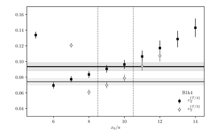
Figure 1: Euclidean time dependence of the two determinations of $c_{\mathrm{\scriptscriptstyle T}}$ for ensemble B1k4 ($\beta=3.512$). The dashed vertical lines enclose the plateau region, the horizontal lines with shaded bands correspond to the plateau values and their respective uncertainties.

The lattice setup to extract $c_{\mathrm{\scriptscriptstyle T}}$ realised here ensures that the initial chiral Ward identity, and thereby also the improvement condition formulae (3.45) and (3.52) implied by it, are imposed on an LCP, along which all physical length scales in correlation functions are kept constant and only the lattice spacing $a$ changes when the bare coupling $g_{0}$ is varied. According to Symanzik’s local effective theory of cutoff effects, the resulting estimates of improvement coefficients such as $c_{\mathrm{\scriptscriptstyle T}}$ are then supposed to exhibit a smooth dependence on $g_{0}^{2}=6/\beta$. As a consequence, any remaining ambiguities in them that could emerge through another choice of LCP or from a different improvement condition will asymptotically disappear towards the continuum limit ($a\to 0$) at a minimum rate $\propto a$. We thus expect our final results for $c_{\mathrm{\scriptscriptstyle T}}(g_{0}^{2})$ to be potentially affected by $\mathrm{O}(a)$ corrections only; however, in view of Eq. (2.18), the latter are beyond the order one is sensitive to in the $\mathrm{O}(a)$ improved theory. Equivalently, any effects of these unavoidable $\mathrm{O}(a)$ ambiguities in hadronic matrix elements or other quantities involving improved (and renormalised) tensor currents will extrapolate to zero in the continuum limit.

The details of our analysis closely follow the similar investigation [45] of $\mathrm{O}(a)$ improvement in the vector channel. Following our experiences there, Eqs. (3.45) and (3.52) are evaluated with two different operator positions $t_{1}=T-t_{2}\in\{T/4,T/3\}$ and averaged over the two central values of $x_{0}$, where $c_{\mathrm{\scriptscriptstyle A}}(g_{0}^{2})$ is taken from Ref. [37], while for the axial and vector currents’ normalisation constants we employ $Z_{\mathrm{\scriptscriptstyle A}}^{\chi}$ and $Z_{\mathrm{\scriptscriptstyle V}}^{\chi}$ calculated within the chirally rotated Schrödinger functional [39], as explained in Section 3.1. The $x_{0}$-dependence of the improvement coefficient on an exemplary ensemble is displayed in Figure 1. Although the local estimator as a function of $x_{0}$ does not develop a clear plateau, as was also observed in similar studies [41, 45], our Ward-identity approach (formulated on the operator level) in conjunction with the LCP setup guarantees that any choice of $x_{0}$ and $t_{1}$ within the $x_{0}$-region furthest from the boundaries is allowed, as long as all physical length scales are kept constant among the different ensembles.

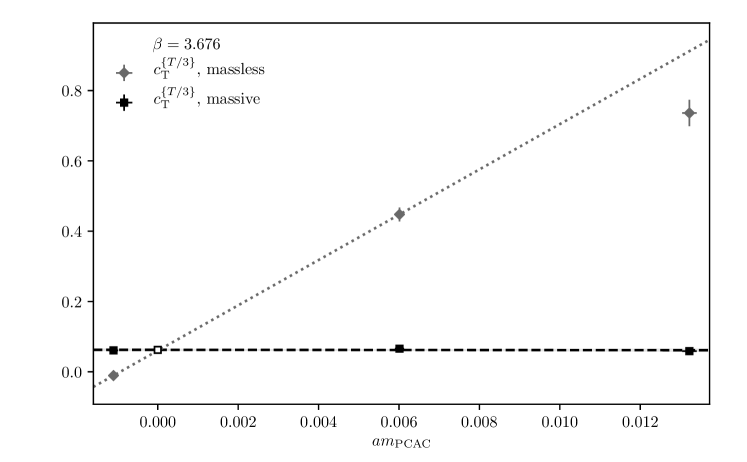
Figure 2: Example of a chiral extrapolation of $c_{\mathrm{\scriptscriptstyle T}}$, here for $c_{\mathrm{\scriptscriptstyle T}}^{\scriptscriptstyle\{T/3\}}$ at $\beta=3.676$, with and without the mass term in the Ward identity (3.45). The dashed lines indicate linear fits to the data, with shaded bands corresponding to the uncertainties of the fits. The open symbol marks the value in the chiral limit.

Figure 2 shows an exemplary extrapolation of $c_{\mathrm{\scriptscriptstyle T}}$ to the chiral limit ($am_{\rm PCAC}\to 0$) for the case of the improvement condition yielding $c_{\mathrm{\scriptscriptstyle T}}^{\scriptscriptstyle\{T/3\}}$ (i.e., the value of $c_{\mathrm{\scriptscriptstyle T}}$ obtained when the operator is inserted at $t_{1}=T/3$), once with the explicit mass term (see Eq. (3.45)) and once without it. Note that our quark mass definition, including the chiral limit as the point of zero sea (and valence) quark masses, is the one based on the partially conserved axial current (PCAC) relation; see Eq. (4.63) in Section 4.2 for its explicit lattice prescription. The mass dependence of the data in Figure 2 illustrates very distinctly that accounting for the mass term in the evaluation of the Ward identity entails an almost flat quark mass dependence and hence a very stable extrapolation. The chirally extrapolated results for the considered variants to extract $c_{\mathrm{\scriptscriptstyle T}}$ are compiled for all ensembles in Table 7 of Appendix B.

In Figure 3 we compare the different sets of results of $c_{\mathrm{\scriptscriptstyle T}}$ from this work with the one-loop prediction for $c_{\mathrm{\scriptscriptstyle T}}$ of Ref. [85] for the tree-level Symanzik-improved (namely, the Lüscher–Weisz) gauge action.

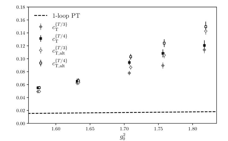
Figure 3: Different determinations of $c_{\mathrm{\scriptscriptstyle T}}$ as a function of the squared bare coupling, $g_{0}^{2}$, in comparison to one-loop perturbation theory [85].

All of our non-perturbative determinations strongly deviate from perturbation theory and approach the one-loop prediction only as $g_{0}\to 0$. In particular, these four variants agree within errors for the two smallest lattice spacings, while they exhibit larger (albeit monotonic) spreads for the coarser ones. This behaviour reinforces that, as argued above, the intrinsic $\mathrm{O}(a)$ ambiguities between determinations based on different improvement conditions vanish smoothly towards the continuum limit, i.e., for $\beta=6/g_{0}^{2}\to\infty$.

In order to settle on a final one among the different, equally admissible determinations labelled as $c_{\mathrm{\scriptscriptstyle T}}^{\scriptscriptstyle\{T/4,T/3\}}$ and $c_{\mathrm{{\scriptscriptstyle T},alt}}^{\scriptscriptstyle\{T/4,T/3\}}$, we consulted the behaviour in the region of weaker couplings: this is motivated by the fact that $c_{\mathrm{\scriptscriptstyle T}}$ is also to be applied in the present context of non-perturbatively solving the scale-dependent renormalisation problem of the tensor current via step-scaling methods in Section 4. For this purpose of evaluating the renormalisation factor $Z_{\mathrm{\scriptscriptstyle T}}(g_{0}^{2},a\mu)$, we specifically need the improvement coefficient at bare couplings $1\lesssim g_{0}^{2}\lesssim 1.7$ considerably smaller than the ones covered by the data discussed so far. Therefore, we have performed an additional simulation at $\beta=8$ and volume $(L^{3}\times T)/a^{4}=16^{3}\times 24$ (allowing relaxation of the LCP condition in this almost perturbative regime), which is to be included as a further constraint in a later interpolation formula for $c_{\mathrm{\scriptscriptstyle T}}(g_{0}^{2})$. In Figure 4 we illustrate the resulting timeslice dependence of the (standard) improvement condition in comparison to the one-loop perturbative prediction [85].

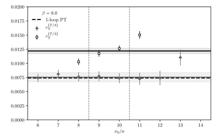
Figure 4: Timeslice dependence of $c_{\mathrm{\scriptscriptstyle T}}$ at $\beta=8$ compared to the one-loop perturbation theory prediction of Ref. [85] (dashed horizontal line). Solid horizontal lines and surrounding shaded areas display the plateau averages and errors of the two non-perturbative estimators with $t_{1}=T/4$ and $t_{1}=T/3$, respectively. The corresponding current quark mass vanishes within error.

While the general picture is very similar to what is encountered in the stronger coupling region, an important observation is that the determination with operator insertion point $t_{1}=T/4$ nicely agrees with the perturbative prediction, whereas $t_{1}=T/3$ shows a significant deviation. Although this is not in disagreement with the theoretical expectation (rather, it must be seen as an $\mathrm{O}(a)$ ambiguity), we eventually chose $c_{\mathrm{{\scriptscriptstyle T},alt}}^{\scriptscriptstyle\{T/4\}}$ as our preferred estimator of $c_{\mathrm{\scriptscriptstyle T}}$, since it exhibits closer agreement with perturbation theory in the weak-coupling regime.

Figure 5 presents the results of our preferred determination of the improvement coefficient of the tensor currents, together with the perturbative prediction and the continuous interpolation of these final non-perturbative results in terms of $g_{0}^{2}$. The fit formula is inspired by the leading term in the perturbative relation between the lattice spacing and the $\beta$-function, $b_{0}=9/(4\pi)^{2}$ being the corresponding universal coefficient for $N_{\mathrm{f}}=3$, constrained by one-loop perturbation theory [85] as $g_{0}^{2}\rightarrow 0$. The $g_{0}^{2}$-dependence in the range covered by the data is best represented by a parametrisation of the form

$$c_{\mathrm{\scriptscriptstyle T}}(g_{0}^{2})=0.00741C_{\mathrm{\scriptscriptstyle F}}g_{0}^{2}\,\Big{[}1+\exp\big{\{}-1/(2b_{0}g_{0}^{2})\big{\}}\big{(}p_{1}+p_{2}g_{0}^{2}\big{)}\Big{]}\,,$$ (3.53a)

with

$$(p_{i}) =\begin{pmatrix}-1.232\\ +1.203\end{pmatrix}\cdot 10^{3}\,, \operatorname{cov}(p_{i},p_{j})=\begin{pmatrix}+17.3880&-10.2809\\ -10.2809&+6.09472\\ \end{pmatrix}\cdot 10^{4}\,.$$ (3.53b)

It describes the five data points at stronger couplings and the weak-coupling data point ($\beta=8$) with $\chi^{2}/{\rm d.o.f.}=0.851$. Let us stress again that this parametrisation and the one-loop behaviour agree almost perfectly up to bare couplings of $g_{0}^{2}\approx 1$, whereas at larger ones a significant departure from perturbation theory is clearly visible.

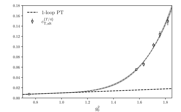
Figure 5: Interpolation formula (3.53) of our preferred determination of $c_{\mathrm{\scriptscriptstyle T}}$ in comparison to one-loop perturbation theory [85].

The interpolation formula (3.53) holds for three-flavour lattice QCD with $\mathrm{O}(a)$ improved Wilson fermions and a tree-level Symanzik-improved gauge action, as also partly employed in the present work. In particular, the bare lattice couplings used here largely overlap with those of the $N_{\mathrm{f}}=2+1$ QCD gauge field configuration ensembles by the CLS collaboration [90, 91, 92, 93, 94], which were generated with exactly this discretisation and provide a broad landscape of pion masses and lattice spacings, aimed to various phenomenological lattice QCD applications. In order to make our results usable within future computations on the CLS ensembles involving $\mathrm{O}(a)$ improved tensor currents, we finally also interpolate (for $\beta=3.85$: slightly extrapolate) our results to the CLS values of $\beta$. These estimates for $c_{\mathrm{\scriptscriptstyle T}}$ are collected in Table 1.

$\beta$	3.34	3.4	3.46	3.55	3.7	3.85
$c_{\mathrm{\scriptscriptstyle T}}$	0.143(5)	0.125(3)	0.110(3)	0.091(2)	0.067(2)	0.051(3)

Table 1: $c_{\mathrm{\scriptscriptstyle T}}$-results for the inverse gauge couplings $\beta$ employed in the $N_{\mathrm{f}}=2+1$ CLS calculations [90, 92, 93]. The errors are the statistical uncertainties propagated from the interpolation formula (3.53), except for $\beta=3.85$, which is slightly outside of the coupling range covered by our data. We thus add 50% of the size of the statistical error in quadrature as a systematic uncertainty to account for this.

4 Renormalisation of $T_{\mu\nu}$

4.1 Renormalisation schemes and strategy

Next, we discuss the renormalisation of the tensor current. Our strategy follows the standard non-perturbative renormalisation and running setup by the ALPHA collaboration, in particular in the context of $N_{\mathrm{f}}=3$ QCD. We define the RGI tensor current following Eq. (2.14),

$$\hat{T}_{\mu\nu}=\overline{T}_{\mu\nu}(\mu)\left[\frac{\overline{g}^{2}(\mu)}{4\pi}\right]^{-\gamma_{\mathrm{\scriptscriptstyle T}}^{(0)}/2b_{0}}\exp\left\{-\int_{0}^{\overline{g}(\mu)}{\rm d}g\left[\frac{\gamma_{\mathrm{\scriptscriptstyle T}}(g)}{\beta(g)}-\frac{\gamma_{\mathrm{\scriptscriptstyle T}}^{(0)}}{b_{0}g}\right]\right\}\,,$$ (4.54)

where $\overline{T}_{\mu\nu}(\mu)$ is the renormalised tensor current in the continuum, $\overline{g}(\mu)$ is some renormalised coupling, $\beta$ and $\gamma_{\mathrm{\scriptscriptstyle T}}$ are the $\beta$-function and the tensor anomalous dimension, respectively, and $b_{0},\gamma_{\mathrm{\scriptscriptstyle T}}^{(0)}$ their leading perturbative coefficients. We shall employ two different mass-independent, finite-volume renormalisation schemes, defined by the renormalisation conditions

$$Z_{\mathrm{\scriptscriptstyle T}}^{\texttt{f}}(g_{0}^{2},a/L)\cdot\frac{k_{\mathrm{\scriptscriptstyle T}}^{\mathrm{I}}(T/2)}{\sqrt{f_{1}}} =\frac{k_{\mathrm{\scriptscriptstyle T}}^{\mathrm{I}}(T/2)}{\sqrt{f_{1}}}\Bigg{|}_{\mbox{\tiny{tree-level}}}\,,$$ (4.55)

$$Z_{\mathrm{\scriptscriptstyle T}}^{\texttt{k}}(g_{0}^{2},a/L)\cdot\frac{k_{\mathrm{\scriptscriptstyle T}}^{\mathrm{I}}(T/2)}{\sqrt{k_{1}}} =\frac{k_{\mathrm{\scriptscriptstyle T}}^{\mathrm{I}}(T/2)}{\sqrt{k_{1}}}\Bigg{|}_{\mbox{\tiny{tree-level}}}\,,$$ (4.56)

where

$$k_{\mathrm{\scriptscriptstyle T}}^{\mathrm{I}}(x_{0})=k_{\mathrm{\scriptscriptstyle T}}(x_{0})+ac_{\mathrm{\scriptscriptstyle T}}\partial_{0}k_{\mathrm{\scriptscriptstyle V}}(x_{0})\,,$$ (4.57)

and the correlation functions $k_{\mathrm{\scriptscriptstyle T}}\equiv\frac{1}{N_{\mathrm{f}}^{2}-1}k_{\mathrm{\scriptscriptstyle T}}^{aa}$ and $k_{\mathrm{\scriptscriptstyle V}}\equiv\frac{1}{N_{\mathrm{f}}^{2}-1}k_{\mathrm{\scriptscriptstyle V}}^{aa}$ have been introduced in Eqs. (3.46) and (3.47). The boundary-to-boundary correlator $k_{1}$, similar to $f_{1}$ introduced in Eq. (3.50), is given by

$$k_{1}=-\frac{1}{6L^{6}}\langle\mathcal{O}^{\prime a}[\gamma_{k}]\mathcal{O}^{a}[\gamma_{k}]\rangle\,.$$ (4.58)

Having at our disposal these non-perturbative renormalisation constants serves two purposes: we can renormalise the tensor current at any given scale $\mu=1/L$ through Eq. (2.24), then trace the renormalisation-group evolution of the current by introducing the step-scaling functions

$$\sigma_{\mathrm{\scriptscriptstyle T}}(u) \equiv\lim_{a\to 0}\Sigma_{\mathrm{\scriptscriptstyle T}}(u,a/L)\equiv\lim_{a\to 0}\left.\frac{Z_{\mathrm{\scriptscriptstyle T}}(g_{0}^{2},a/(2L))}{Z_{\mathrm{\scriptscriptstyle T}}(g_{0}^{2},a/L)}\right|_{u=\overline{g}^{2}(1/L)}=\exp\left\{\int_{\bar{g}(L^{-1})}^{\bar{g}((2L)^{-1})}\kern-10.0pt\mathrm{d}g\frac{\gamma_{\mathrm{\scriptscriptstyle T}}(g)}{\beta(g)}\right\}\,.$$ (4.59)

By computing $\Sigma_{\mathrm{\scriptscriptstyle T}}^{\texttt{f}}(u,a/L)$ and $\Sigma_{\mathrm{\scriptscriptstyle T}}^{\texttt{k}}(u,a/L)$ at several values of $u$ and $a/L$ it is possible to obtain the respective continuum versions $\sigma_{\mathrm{\scriptscriptstyle T}}^{\texttt{f}/\texttt{k}}(u)$, and hence $\gamma_{\mathrm{\scriptscriptstyle T}}^{\texttt{f}/\texttt{k}}$, non-perturbatively for a wide range of scales. Recall that the step-scaling function is a particular case of the general solution of the RGE (2.4) in terms of an RG evolution operator $U(\mu_{2},\mu_{1})$, viz.

$$\overline{\mathcal{O}}(\mu_{2})=U(\mu_{2},\mu_{1})\overline{\mathcal{O}}(\mu_{1})\,;\qquad U(\mu_{2},\mu_{1})=\exp\left\{\int_{\bar{g}(\mu_{1})}^{\bar{g}(\mu_{2})}\kern-5.0pt\mathrm{d}g\frac{\gamma_{\mathcal{O}}(g)}{\beta(g)}\right\}\,,$$ (4.60)

so that $\sigma_{\mathrm{\scriptscriptstyle T}}(u)=U(\bar{g}((2L)^{-1}),\bar{g}(L^{-1}))$ with $u=\bar{g}(L^{-1})$ and the appropriate anomalous dimension $\gamma_{\mathrm{\scriptscriptstyle T}}$ of the tensor operator used in Eq. (4.60).

In order to determine the anomalous dimension, we shall follow the same strategy as for quark masses [32]. Using the notation in Eqs. (2.4) and (4.60), we factorise Eq. (2.14) as

$$\begin{split}\hat{T}_{\mu\nu}&=\hat{c}(\mu_{\mathrm{had}})\overline{T}_{\mu\nu}(\mu_{\mathrm{had}})\\ &=\underbrace{\hat{c}(\mu_{\rm\scriptscriptstyle PT})}_{\text{PT}}\,\underbrace{U(\mu_{\rm\scriptscriptstyle PT},\mu_{0}/2)}_{\text{SF}}\,\underbrace{U(\mu_{0}/2,\mu_{\mathrm{had}})}_{\text{GF}}\,\overline{T}_{\mu\nu}(\mu_{\mathrm{had}})\,,\end{split}$$ (4.61)

where $\mu_{\mathrm{had}}$ is a low-energy scale of the order of $\Lambda_{\rm\scriptscriptstyle QCD}$, $\mu_{\rm\scriptscriptstyle PT}$ is some high-energy scale, of the order of the electroweak scale, where perturbation theory is safe (next-to-leading-order predictions are available in our case), $\mu_{0}$ is an intermediate scale of the order of $4\,{\rm GeV}$, and the factors labelled “GF” and “SF” are computed using gradient-flow and SF non-perturbative couplings, respectively (see Ref. [32] for a detailed explanation, a full reference list, and any unexplained notation). The key points in the whole setup are that each of these factors, except for the first one, can be computed non-perturbatively and taken to the continuum limit with fully controlled systematics, and that the connection to the RGI allows one to match the result to any other renormalisation scheme convenient for phenomenology.

4.2 RG running at high energies

In the high-energy regime we have performed simulations at eight values of the renormalised SF coupling

$$u_{\mathrm{\scriptscriptstyle SF}} =\{1.1100,1.1844,1.2656,1.3627,1.4808,1.6173,1.7943,2.0120\}\,,$$ (4.62)

using the Wilson plaquette action [95] and an $\mathrm{O}(a)$-improved Wilson fermion action [30], with the non-perturbative value for $c_{\mathrm{sw}}$ from Ref. [96] and one-loop [97] and two-loop [98] values for the boundary improvement coefficients $\tilde{c}_{\mathrm{t}}$ and $c_{\mathrm{t}}$, respectively. Simulations are performed at three different values of the (inverse) lattice spacing $L/a=6,8,12$, except for the strongest coupling $u_{\mathrm{\scriptscriptstyle SF}}=2.012$ where a fourth, finer lattice spacing $L/a=16$ is used ($L$ is implicitly fixed through $u$). The three quarks in all simulations are tuned to be massless by demanding that the PCAC mass,

$$m(g_{0}^{2},\kappa)=\left.\frac{{1\over 2}(\partial_{0}^{*}+\partial_{0}^{\phantom{*}})f_{\rm A}(x_{0})+ac_{\mathrm{\scriptscriptstyle A}}\partial_{0}^{*}\partial_{0}^{\phantom{*}}f_{\rm\scriptscriptstyle P}(x_{0})}{2f_{\rm P}(x_{0})}\right|_{x_{0}=T/2}\,,$$ (4.63)

vanishes, using the improvement coefficient $c_{\mathrm{\scriptscriptstyle A}}(g_{0}^{2})=-0.005680(2)C_{\mathrm{\scriptscriptstyle F}}g_{0}^{2}$ to one-loop order in perturbation theory [97, 28]. All simulations were performed with a variant of the openQCD code [99].

Since our computation of the improvement coefficient $c_{\mathrm{\scriptscriptstyle T}}$ is available only for tree-level Symanzik-improved gauge action, we use its one-loop value for the plaquette gauge action, determined in Ref. [28]. Note that this is not expected to have a major impact, since the lattices employed in the high-energy region are very close to the continuum limit and the residual $O(ag_{0}^{4})$ cutoff effects should be highly suppressed. Furtheremore, the step-scaling functions $\Sigma_{\mathrm{\scriptscriptstyle T}}$ obtained from these simulations are corrected by subtracting the cutoff effects to all orders in $a$ and leading order in $g_{0}^{2}$, as described in Ref. [29, Sec. 4.2].

4.2.1 Determination of the anomalous dimension

$n_{s}$	$n_{\rho}$	$\hat{c}^{\texttt{f}}(\mu_{0}/2)$	$\chi^{2}/\mathrm{d.o.f.}$
2	2	1.1324(64)	19.77 / 15
2	3	1.1213(74)	11.30 / 14
3	2	1.1093(97)	10.31 / 14
3	3	1.112(11)	10.03 / 13

$n_{s}$	$n_{\rho}$	$\hat{c}^{\texttt{k}}(\mu_{0}/2)$	$\chi^{2}/\mathrm{d.o.f.}$
2	2	1.1670(55)	15.95 / 15
2	3	1.1586(63)	8.96 / 14
3	2	1.1498(84)	8.96 / 14
3	3	1.1532(96)	8.43 / 13

Table 2: Different fits of the anomalous dimension and the resulting values of the running factor $\hat{c}(\mu_{0}/2)$, cf. Eq. (2.14). We quote results for both the f-scheme (left) and the k-scheme (right), with our preferred fit result highlighted.

To determine the anomalous dimension of the tensor current in the high-energy regime we make use of a global fit procedure which combines the continuum extrapolation at individual values of the strong coupling with a direct fit to the anomalous dimension constrained by the expectation from perturbation theory. Both our starting expression, and the fitting strategy, follow a similar reasoning as the one discussed at length in Ref. [32] for the similar case of the running quark mass.

Our starting expression to model $\Sigma_{\mathrm{\scriptscriptstyle T}}^{\mathrm{I}}$ is

$$\Sigma_{\mathrm{\scriptscriptstyle T}}^{\mathrm{I}}(u,a/L) =\exp\left(\int_{\sqrt{u}}^{\sqrt{\sigma(u)}}\mathrm{d}x\frac{\gamma_{\mathrm{\scriptscriptstyle T}}(x)}{\beta(x)}\right)+\left(\sum_{n=2}^{n_{\rho}}\rho_{n}u^{n}\right)\bigg{(}\frac{a}{L}\bigg{)}^{2}\,.$$ (4.64)

For the anomalous dimension, we use the asymptotic expansions (2.8) as our ansatz,

$$\gamma_{\mathrm{\scriptscriptstyle T}}(x) =-x^{2}\sum_{n=0}^{n_{s}}t_{n}x^{2n}\,.$$ (4.65)

We try fitting with different values for $n_{s}$ and $n_{\rho}$ and find consistent results as detailed in Table 2. For our final result, we quote the fits with $n_{s}=2$, $n_{\rho}=3$. For the scheme labelled f the parameters are given by

$$t_{0}^{\texttt{f}} =\frac{8}{3(4\pi)^{2}}\equiv\gamma_{\mathrm{\scriptscriptstyle T}}^{(0)}\,, t_{1}^{\texttt{f}} =0.00627445\equiv\gamma_{\mathrm{\scriptscriptstyle T}}^{(1),\texttt{f}}\,, t_{2}^{\texttt{f}} =+0.00073(25)\,,$$ (4.66)

with $$\chi^{2}/\mathrm{d.o.f.}=0.807$$, while for the scheme labelled k we obtain

$$t_{0}^{\texttt{k}} =\frac{8}{3(4\pi)^{2}}\equiv\gamma_{\mathrm{\scriptscriptstyle T}}^{(0)}\,, t_{1}^{\texttt{k}} =0.00579501\equiv\gamma_{\mathrm{\scriptscriptstyle T}}^{(1),\texttt{k}}\,, t_{2}^{\texttt{k}} =-0.00022(21)\,,$$ (4.67)

with $\chi^{2}/\mathrm{d.o.f.}=0.640$.

In Figure 6 the non-perturbative anomalous dimensions are compared to the corresponding one-loop and two-loop perturbative predictions. For the scheme labelled k the non-perturbative result agrees with the two-loop prediction within errors while the discrepancy for the scheme labelled f corresponds to several standard errors.

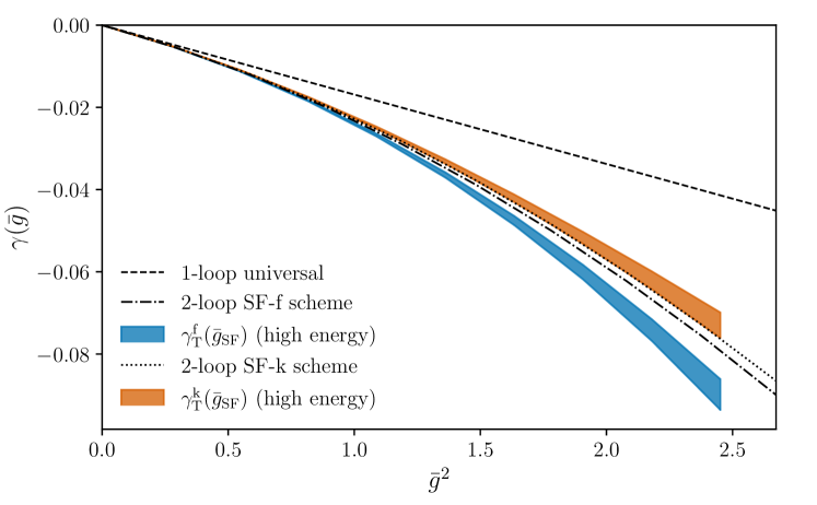
Figure 6: Non-perturbative anomalous dimension of the tensor current in the two SF schemes in the high-energy region. Perturbative expectations are shown for comparison.

Having determined the anomalous dimension, which is constrained by construction to make contact with two-loop perturbation theory at high energies, it is then possible to determine directly the factor $\hat{c}(\mu_{0}/2)=\hat{c}(\mu_{\rm\scriptscriptstyle PT})U(\mu_{\rm\scriptscriptstyle PT},\mu_{0}/2)$ in Eq. (4.61), in a way that makes it insensitive to any specific prescription for $\mu_{\rm\scriptscriptstyle PT}$—see Ref. [32] for details. We quote for our two schemes

$$\hat{c}^{\mathrm{\texttt{f}}}(\mu_{0}/2) =1.1213(74)\,, \hat{c}^{\mathrm{\texttt{k}}}(\mu_{0}/2) =1.1586(63)\,.$$ (4.68)

4.3 RG running at low energies

Below the matching scale $\mu_{0}/2$ we employ the GF scheme, for which we have performed simulations at bare parameters such that the GF coupling is close to one of the following seven values

$$u_{\mathrm{\scriptscriptstyle GF}} \approx\{{2.12,2.39,2.73,3.20,3.86,4.49,5.29}\}\,.$$ (4.69)

These simulations are performed at three lattice spacings $L/a=8,12,16$, again using non-perturbatively $\mathrm{O}(a)$ improved Wilson fermions but now with a tree-level Symanzik-improved gauge action [100]. The value of $c_{\rm sw}$ has been determined in Ref. [101]. The chiral point is tuned as in the SF regime via the PCAC relation in Eq. (4.63), with the corresponding non-perturbative value of $c_{\mathrm{\scriptscriptstyle A}}$ [37]. In this case, our non-perturbative results for $c_{\mathrm{\scriptscriptstyle T}}$ from Section 3 are actually utilised to ${\rm O}(a)$ improve the tensor current. All computations are carried out at fixed topological charge $Q=0$ by projecting onto the trivial topological sector, as explained in Ref. [31].

4.3.1 Boundary improvement

One relevant source of systematic uncertainty comes from the fact that the $\mathrm{O}(a)$ improvement coefficients $c_{\mathrm{t}}$ and $\tilde{c}_{\mathrm{t}}$, associated to boundary counterterms in the SF setup, are only known within perturbation theory. For the tree-level Symanzik-improved gauge action they are actually only known to one-loop from Refs. [102, 103]. While the impact of the perturbative truncation is negligible at small values of $u$, it may become relevant in the low-energy region of the running. This effect was studied in Ref. [32] for the case of the running mass, and turned out to be negligible within statistical uncertainties in the computation of the renormalisation constant $Z_{\mathrm{\scriptscriptstyle P}}$. However, in the case of the dependence on $\tilde{c}_{\mathrm{t}}$, to which fermionic correlation functions are most sensitive, an accidental cancellation pushes the perturbative truncation effect on $Z_{\mathrm{\scriptscriptstyle P}}$ one order further in $g_{0}^{2}$. This does not happen in the case of $Z_{\mathrm{\scriptscriptstyle T}}$, meaning that we have to reassess the issue here.

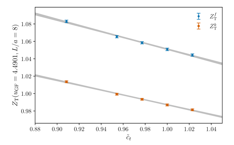
Figure 7: Dependence of the tensor renormalisation constant $Z_{\mathrm{\scriptscriptstyle T}}$ on $\tilde{c}_{\mathrm{t}}$ for the f-scheme (circles) and the k-scheme (diamonds) at $u_{\mathrm{\scriptscriptstyle GF}}=4.4901$ on $L/a=8$ lattices.

To that effect, we have performed additional simulations at $u=4.4901$ and $L/a=8$, where we vary $c_{\mathrm{t}}$ and $\tilde{c}_{\mathrm{t}}$ independently. For $c_{\mathrm{t}}$ we find a very mild dependence on the value used in the simulation, and proceed to neglect that source of uncertainty. However, for $\tilde{c}_{\mathrm{t}}$ we find a fairly strong dependence, as can be seen from Figure 7. In order to account for this effect by including an estimate of the systematic uncertainty incurred in, we follow the same reasoning as in Ref. [32]: linear error propagation suggests that the effect of a shift $\delta\tilde{c}_{\mathrm{t}}$ on the value of $Z_{\mathrm{\scriptscriptstyle T}}$ will have the form

$$\delta_{\tilde{c}_{\mathrm{t}}}Z_{\mathrm{\scriptscriptstyle T}}\approx\left|\frac{\partial Z_{\mathrm{\scriptscriptstyle T}}}{\partial\tilde{c}_{\mathrm{t}}}\right|\delta\tilde{c}_{\mathrm{t}}\,.$$ (4.70)

The slope $\partial Z_{\mathrm{\scriptscriptstyle T}}/\partial\tilde{c}_{\mathrm{t}}$ at $u=4.4901$ can be extracted from a linear fit to our $L/a=8$ data, as depicted in Figure 7. In order to estimate the effect at a different value of $u$ and/or $L/a$, we posit the scaling law

$$\frac{\partial Z_{\mathrm{\scriptscriptstyle T}}}{\partial\tilde{c}_{\mathrm{t}}}\approx\xi u\frac{a}{L}\,,$$ (4.71)

where $\xi$ is some constant coefficient. The rationale is that the slope has a leading behaviour proportional to $g_{0}^{2}$ in perturbation theory, and, the effect being associated to an $\mathrm{O}(a)$ improvement counterterm, it is expected to vanish linearly in $a$ at small values of the lattice spacing. By applying this to the result of our linear fit, we estimate:

$$\xi^{\texttt{f}}=-0.601(25)\,,\quad\xi^{\texttt{k}}=-0.502(19)\,.$$ (4.72)

Finally, in order to apply Eq. (4.70) we conservatively use a value of the shift $\delta\tilde{c}_{\mathrm{t}}$ corresponding to 100% of the one-loop perturbative deviation from the tree-level value $\tilde{c}_{\mathrm{t}}=1$. Note that, at the level of the step-scaling function $\Sigma_{\mathrm{\scriptscriptstyle T}}$, our modelling of the uncertainty leads to

$$\frac{\delta_{\tilde{c}_{\mathrm{t}}}\Sigma_{\mathrm{\scriptscriptstyle T}}}{\Sigma_{\mathrm{\scriptscriptstyle T}}} \approx\left|\frac{\sigma(u)}{2Z_{\mathrm{\scriptscriptstyle T}}(2L)}-\frac{u}{Z_{\mathrm{\scriptscriptstyle T}}(L)}\right||\xi|\frac{a}{L}\delta\tilde{c}_{\mathrm{t}}\,,$$ (4.73)

which implies that the uncertainty affecting the values of $Z_{\mathrm{\scriptscriptstyle T}}$ that enter the ratio undergoes a partial cancellation, making $\Sigma_{\mathrm{\scriptscriptstyle T}}$ less sensitive to this effect than $Z_{\mathrm{\scriptscriptstyle T}}$ itself.

The resulting systematic uncertainty induced in $\Sigma_{\mathrm{\scriptscriptstyle T}}$ is quoted as the second number in parentheses in the relevant tables of Appendix C. Note that it is largely subdominant with respect to the statistical uncertainty, save for a few $L/a=8~{}\to~{}16$ steps where it is still smaller but of comparable size. In the case of $Z_{\mathrm{\scriptscriptstyle T}}$, on the other hand, the systematic uncertainty can be sizeable, which will be commented upon below when the matching at a hadronic scale is discussed.

4.3.2 Determination of the anomalous dimension

To determine the anomalous dimension in the low-energy region we once again make use of a global fit procedure, which in this case is strictly necessary as the values of the GF coupling $u_{\mathrm{\scriptscriptstyle GF}}$ are not exactly tuned to a constant for different values of $L/a$. The ratios of RG functions are parametrised as

$$f(x) =\frac{\gamma_{\mathrm{\scriptscriptstyle T}}(x)}{\beta(x)}=\frac{1}{x}\sum_{n=0}^{n_{r}}f_{n}x^{2n}\,,$$ (4.74)

and we perform a global fit to the relation

$$\Sigma_{\mathrm{\scriptscriptstyle T}}(u,a/L) =\exp\left(\int_{\sqrt{u}}^{\sqrt{\Sigma(u,a/L)}}\mathrm{d}xf(x)\right)+\left(\sum_{n=n_{\rho,\mathrm{start}}}^{n_{\rho,\mathrm{stop}}}\rho_{n}u^{n}\right)(a/L)^{2}$$ (4.75)

$$=\exp\left(\bigg{[}f_{0}\log(x)+\sum_{n=1}^{n_{r}}f_{n}\frac{x^{2n}}{2n}\bigg{]}_{\sqrt{u}}^{\sqrt{\Sigma(u,a/L)}}\right)+\left(\sum_{n=n_{\rho,\mathrm{start}}}^{n_{\rho,\mathrm{stop}}}\rho_{n}u^{n}\right)(a/L)^{2}\,,$$ (4.76)

to obtain the parameters $f_{n}$. For our best fits with $n_{r}=2$, $n_{\rho,\mathrm{start}}=1$ and $n_{\rho,\mathrm{stop}}=2$ we obtain the running factors

$$U^{\texttt{f}}(\mu_{0}/2,\mu_{\mathrm{had}}) =0.6475(59)\,, U^{\texttt{k}}(\mu_{0}/2,\mu_{\mathrm{had}}) =0.7519(45)\,.$$ (4.77)

With these parameters, we can also reconstruct the anomalous dimension via the relation

$$\gamma_{\mathrm{\scriptscriptstyle T}}(\bar{g}) =-\bar{g}^{2}\frac{\sum_{n=0}^{n_{r}}f_{n}\bar{g}^{2n}}{\sum_{k=0}^{k_{t}}p_{k}\bar{g}^{2n}}\,,$$ (4.78)

where the $\beta$-function is parametrised as in Eq. (4.12) of Ref. [31]. For our best fits we obtain

$$f_{0}^{\texttt{f}} =0.326(63)\,, f_{1}^{\texttt{f}} =0.050(31)\,, f_{2}^{\texttt{f}} =+0.0035(34)\,,$$ (4.79)

with $$\chi^{2}/\mathrm{d.o.f.}=0.831$$, and

$$f_{0}^{\texttt{k}} =0.298(47)\,, f_{1}^{\texttt{k}} =0.043(22)\,, f_{2}^{\texttt{k}} =-0.0021(24)\,,$$ (4.80)

with $\chi^{2}/\mathrm{d.o.f.}=1.130$. The corresponding covariance matrices can be found in Section A.1. The curves obtained from these fits are shown in Figure 8, together with those derived in the high-energy regime, and with the one-loop prediction.

The overall effect of the systematic error related to $\tilde{c}_{\mathrm{t}}$ to the total squared error of the running factor in the low-energy regime, taken into account via the procedure described in Section 4.3.1, corresponds to about $4\%$ for both schemes.

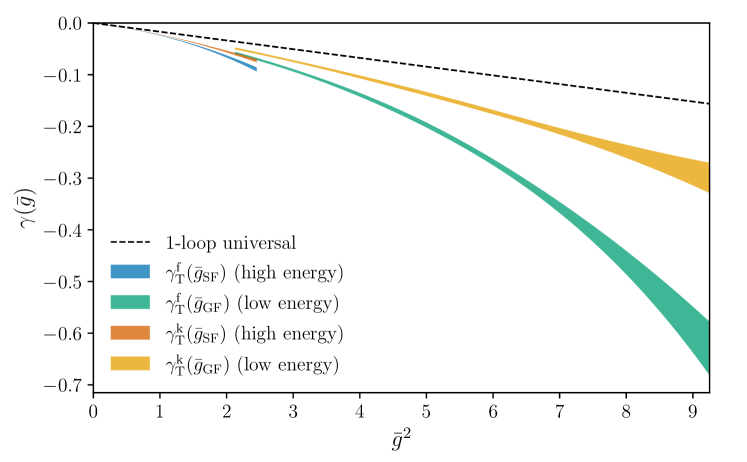
Figure 8: Non-perturbative anomalous dimension of the tensor current in the two schemes. The perturbative one-loop expectation is shown for comparison. See Figure 6 for a close up of the SF region.

4.4 Matching at a hadronic scale

As the final step in our renormalisation strategy, we need to compute the renormalisation constant $Z_{\mathrm{\scriptscriptstyle T}}$ at a fixed hadronic scale $\mu_{\mathrm{had}}=1/L_{\mathrm{had}}$ for changing bare couplings $g_{0}^{2}$ which match the couplings used in large-volume simulations. In practice, we aim at the interval $\beta\in[3.40,3.85]$ used by the CLS consortium. The hadronic scale is fixed by a $L/a=20$ lattice with $\beta=3.79$, resulting in $u_{\mathrm{had}}=9.25$. Using the scale setting of Ref. [91], this corresponds to an energy scale $\mu_{\mathrm{had}}=233(8)\,{\rm MeV}$. Lattices with $L/a=24,16,12,10$ were then tuned to match this scale covering the range of CLS couplings.

$L/a$	$\beta$	$\kappa$	$u_{\mathrm{\scriptscriptstyle GF}}$	$Lm$	$Z_{\mathrm{\scriptscriptstyle T}}^{\texttt{f}}(g_{0}^{2},a\mu_{\mathrm{had}})$	$N_{\rm ms}$
10	3.400000	0.136804	9.282(40)	$-0.0236(35)$	1.308(6)(15)	2489
10	3.411000	0.136765	9.290(31)	$+0.0189(22)$	1.276(4)(15)	4624
12	3.480000	0.137039	9.417(43)	$-0.0115(31)$	1.328(7)(12)	1868
12	3.488000	0.137021	9.393(40)	$+0.0035(24)$	1.329(6)(12)	2667
12	3.497000	0.137063	9.118(51)	$-0.0102(28)$	1.318(8)(12)	1491
16	3.629800	0.137163	9.638(35)	$-0.0062(12)$	1.3955(81)(90)	6362
16	3.649000	0.137158	9.417(36)	$-0.0024(14)$	1.4016(91)(88)	4837
16	3.657600	0.137154	9.169(43)	$-0.0039(15)$	1.3818(90)(85)	3262
16	3.671000	0.137148	9.045(54)	$+0.0009(24)$	1.371(12)(8)	1553
20	3.790000	0.137048	9.256(36)	$-0.00053(99)$	1.4105(75)(66)	4305
24	3.893412	0.136894	9.370(61)	$-0.00001(100)$	1.471(14)(5)	3008
24	3.912248	0.136862	9.132(49)	$+0.00010(76)$	1.430(12)(5)	5086

Table 3: Results for $Z_{\mathrm{\scriptscriptstyle T}}$ in the hadronic matching region (f-scheme). The first error is statistical, the second is systematic due to the use of a one-loop result for the improvement coefficient $\tilde{c}_{\mathrm{t}}$.

$L/a$	$\beta$	$\kappa$	$u_{\mathrm{\scriptscriptstyle GF}}$	$Lm$	$Z_{\mathrm{\scriptscriptstyle T}}^{\texttt{k}}(g_{0}^{2},a\mu_{\mathrm{had}})$	$N_{\rm ms}$
10	3.400000	0.136804	9.282(40)	$-0.0236(35)$	1.109(4)(12)	2489
10	3.411000	0.136765	9.290(31)	$+0.0189(22)$	1.089(3)(12)	4624
12	3.480000	0.137039	9.417(43)	$-0.0115(31)$	1.116(4)(10)	1868
12	3.488000	0.137021	9.393(40)	$+0.0035(24)$	1.117(3)(10)	2667
12	3.497000	0.137063	9.118(51)	$-0.0102(28)$	1.1141(44)(98)	1491
16	3.629800	0.137163	9.638(35)	$-0.0062(12)$	1.1546(32)(75)	6362
16	3.649000	0.137158	9.417(36)	$-0.0024(14)$	1.1586(37)(73)	4837
16	3.657600	0.137154	9.169(43)	$-0.0039(15)$	1.1527(39)(71)	3262
16	3.671000	0.137148	9.045(54)	$+0.0009(24)$	1.1452(48)(70)	1553
20	3.790000	0.137048	9.256(36)	$-0.00053(99)$	1.1697(37)(55)	4305
24	3.893412	0.136894	9.370(61)	$-0.00001(100)$	1.2060(66)(45)	3008
24	3.912248	0.136862	9.132(49)	$+0.00010(76)$	1.1905(50)(44)	5086

Table 4: Results for $Z_{\mathrm{\scriptscriptstyle T}}$ in the hadronic matching region (k-scheme). The first error is statistical, the second is systematic due to the use of a one-loop result for the improvement coefficient $\tilde{c}_{\mathrm{t}}$.

The full set of simulations in the hadronic regime is summarised in Tables 3 and 4. The tuning in both the coupling $u_{\mathrm{\scriptscriptstyle GF}}$ and the mass $Lm$ is only precise up to a few standard deviations; we account for this effect by performing a combined fit of the data as a function of $g_{0}^{2}$, $u_{\mathrm{\scriptscriptstyle GF}}$ and $Lm$, in order to extract $Z_{\mathrm{\scriptscriptstyle T}}(g_{0}^{2},a\mu_{\mathrm{had}})$ on our line of constant physics defined by $u_{\mathrm{had}}=\bar{g}^{2}(\mu_{\mathrm{had}})=9.25$, $Lm=0$. As a model for our data we use the fit form

$$\begin{split}Z_{\mathrm{\scriptscriptstyle T}}(g_{0}^{2},u_{\mathrm{\scriptscriptstyle GF}},Lm)&=Z_{\mathrm{\scriptscriptstyle T}}(g_{0}^{2},a\mu_{\mathrm{had}})+t_{10}\,(u_{\mathrm{\scriptscriptstyle GF}}-u_{\mathrm{had}})+t_{01}\,Lm\,,\\ Z_{\mathrm{\scriptscriptstyle T}}(g_{0}^{2},a\mu_{\mathrm{had}})&=z_{0}+z_{1}(\beta-\beta_{0})+z_{2}(\beta-\beta_{0})^{2}\,.\end{split}$$ (4.81)

For the free coefficients we obtain

$$z_{0}^{\texttt{f}} =1.4178(75)\,, z_{1}^{\texttt{f}} =0.263(38)\,, z_{2}^{\texttt{f}} =-0.21(10)\,,$$ (4.82)

with $\chi^{2}/\mathrm{d.o.f.}=0.621$, and

$$z_{0}^{\texttt{k}} =1.1748(58)\,, z_{1}^{\texttt{k}} =0.191(21)\,, z_{2}^{\texttt{k}} =-0.043(55)\,,$$ (4.83)

with $\chi^{2}/\mathrm{d.o.f.}=0.437$. The corresponding functions and data points are presented in Figure 9 and their covariances can be found in Section A.2. In Table 5 we quote the values of $Z_{\mathrm{\scriptscriptstyle T}}$ at $\mu_{\mathrm{had}}$ for the values of $\beta$ where CLS ensembles have been simulated.

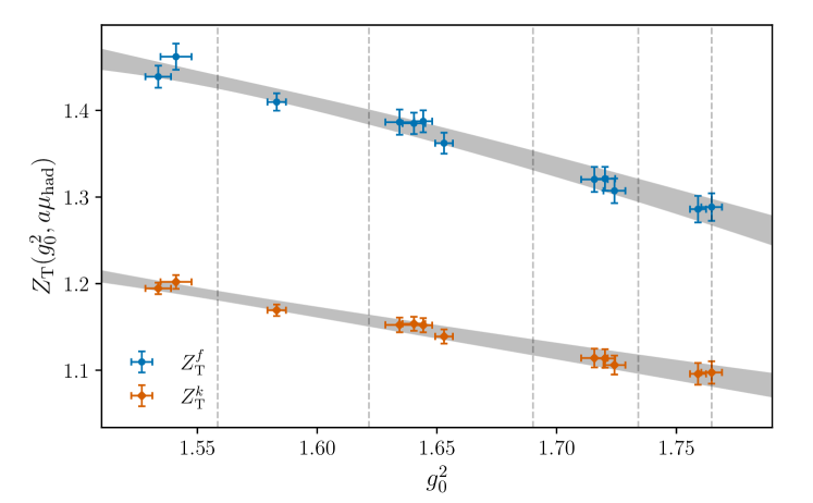
Figure 9: Tensor current renormalisation factor at the hadronic matching point $u_{\mathrm{had}}=9.25$ in the f-scheme (circles) and the k-scheme (diamonds). Dashed lines indicate the bare gauge couplings used in CLS simulations.

Note that, as hinted before, the systematic uncertainty due to the use of a one-loop result for the improvement coefficient $\tilde{c}_{\mathrm{t}}$, that we conservatively estimate via Eq. (4.70), turns out to be substantial. It is indeed dominant with respect to the statistical uncertainty, except for the largest $L/a=24$ lattices. At the level of fit coefficients, the error on the zeroth fit parameter is dominated by the systematic error estimate (77% for f and 88% for k) while the contribution is subleading for the remaining parameters (10% and 5% for f, 24% and 11% for k). Note also that systematic uncertainties are $100\%$ correlated by construction, and should be treated in that way when the values of $Z_{\mathrm{\scriptscriptstyle T}}$ quoted are employed.

4.5 Total running and renormalisation factors

We are now in a position to quote our final results. The total running factors relating RGI operator insertions to renormalised insertions at $\mu_{\mathrm{had}}$ are given by the products of the two running factors in Eqs. (4.68) and (4.77). They are found to be

$$\hat{c}^{\texttt{f}}(\mu_{\mathrm{had}}) =0.7260(81)(14)\,, \hat{c}^{\texttt{k}}(\mu_{\mathrm{had}}) =0.8711(70)(11)\,,$$ (4.84)

where the first error is statistical and the second is the systematic error resulting from the fact that we only know the boundary $\mathrm{O}(a)$ improvement coefficients perturbatively. We stress that these are continuum quantities, where the only dependence left is in the renormalisation scheme. We also stress that, as in the case of the values of $Z_{\mathrm{\scriptscriptstyle T}}$ at $\mu_{\mathrm{had}}$, systematic uncertainties are $100\%$ correlated by construction, and should be treated in that way when the values of the above running factors are used.

By combining the running factors in Eq. (4.84) with the renormalisation constants at $\mu_{\mathrm{had}}$ discussed in Section 4.4, it is furthermore possible to introduce a total renormalisation factor that connects bare and RGI operator insertions, viz.

$$\hat{Z}_{\mathrm{\scriptscriptstyle T}}(g_{0}^{2}) \equiv\hat{c}(\mu_{\mathrm{had}})Z_{\mathrm{\scriptscriptstyle T}}(g_{0}^{2},a\mu_{\mathrm{had}})\;.$$ (4.85)

This is a divergent quantity as $a\to 0$, which depends on the bare coupling only, since the dependence on the hadronic matching scale $\mu_{\mathrm{had}}$ cancels by construction up to cutoff effects. By the same reason, and because the RGI is unique, the values of $\hat{Z}_{\mathrm{\scriptscriptstyle T}}$ computed through the two schemes can only differ by cutoff effects; in particular, $\hat{Z}_{\mathrm{\scriptscriptstyle T}}^{\texttt{f}}(g_{0}^{2})/\hat{Z}_{\mathrm{\scriptscriptstyle T}}^{\texttt{k}}(g_{0}^{2})=1+\mathrm{O}(a^{2})$ (up to logarithmic corrections). The value of $\hat{Z}_{\mathrm{\scriptscriptstyle T}}$ within the range in $g_{0}^{2}$ covered by our simulations can be obtained trivially by multiplying the coefficients in Eqs. (4.82) and (4.83) by the corresponding factors in Eq. (4.84). Figure 10 shows a comparison of the total renormalisation factor in both schemes as a function of the bare gauge coupling. The same comments as above regarding the correlation of systematic uncertainties apply.

$\beta$	$Z_{\mathrm{\scriptscriptstyle T}}^{\texttt{f}}(g_{0}^{2},a\mu_{\mathrm{had}})$	$Z_{\mathrm{\scriptscriptstyle T}}^{\texttt{k}}(g_{0}^{2},a\mu_{\mathrm{had}})$
3.40	1.283(4)(15)	1.094(3)(12)
3.46	1.308(3)(13)	1.107(2)(11)
3.55	1.342(3)(11)	1.1265(18)(90)
3.70	1.3924(37)(78)	1.1573(19)(65)
3.85	1.4328(50)(59)	1.1861(25)(49)

Table 5: Results for $Z_{\mathrm{\scriptscriptstyle T}}(g_{0}^{2},a\mu_{\mathrm{had}})$ at CLS $\beta$-values for both schemes. The first error is statistical, the second is systematic due to the use of a one-loop result for the improvement coefficient $\tilde{c}_{\mathrm{t}}$.

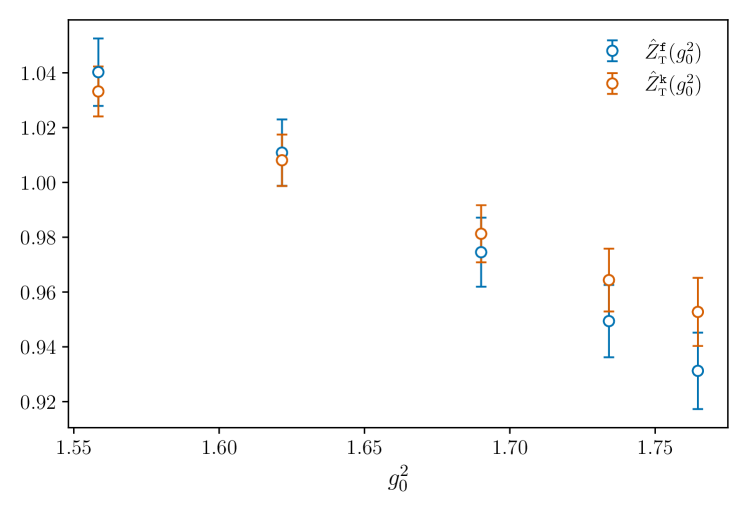
Figure 10: Comparison of the total renormalisation factors $\hat{Z}_{\mathrm{\scriptscriptstyle T}}(g_{0}^{2})$ at the CLS couplings for both schemes. Note that the errors are highly correlated as all values for a given scheme share the running factor $\hat{c}$, whose uncertainty is dominant.

5 Conclusions

In the present work, we computed the renormalisation and running of non-singlet quark bilinears with tensorial Lorentz structure, thereby addressing the last missing non-trivial anomalous dimensions of two- and four-quark operators within the ALPHA collaboration’s $N_{\mathrm{f}}=3$ renormalisation programme. Our approach, which is based on step scaling in the Schrödinger functional and gradient flow schemes, allowed us to non-perturbatively compute the operator anomalous dimension from the hadronic scale $\mu_{\mathrm{had}}=233(8)$ MeV all the way up to electroweak energies, in two different renormalisation schemes. As an accessory step, we computed non-perturbatively the improvement coefficient $c_{\mathrm{\scriptscriptstyle T}}$, required to obtain ${\rm O}(a)$ improved tensor currents in the chiral limit, which is also relevant for computations of ${\rm O}(a)$ improved amplitudes involving the latter. In this procedure all error sources, statistical and systematic, are kept under control.

The main results provided in the text are:

• The non-perturbative values of the improvement coefficient $c_{\mathrm{\scriptscriptstyle T}}(g_{0}^{2})$ for a non-perturbatively ${\rm O}(a)$ improved fermion action and a tree-level Symanzik improved gauge action, in a large range of values of the bare gauge coupling that includes those employed in large volume simulations (cf. Eq. (3.53) and Table 1).

• The RG running factor connecting amplitudes of tensor currents at the hadronic scale $\mu_{\mathrm{had}}$ and the corresponding RGI value, Eq. (4.84). These are continuum quantities, that only depend on the renormalisation scheme. Results are provided in two different SF schemes for better control of the systematics, with a ballpark 1% precision. It is important to point out that the running factors are in the continuum limit, and can therefore be applied to continuum results obtained with any lattice action.

• The renormalisation constants of the improved currents in the range of couplings relevant for CLS simulations, as well as the total renormalisation factor relating bare and RGI hadronic matrix elements (cf. Eq. (4.81), Table 5). These results are regularisation dependent, but still wide-ranging, since any computation based on CLS ensembles can benefit from them.

Some interesting aspects of our results are worth stressing. One is that the non-perturbative anomalous dimensions of tensor currents seem to have generally larger values, and more sizeable deviations from low-order perturbation theory, than the other independent anomalous dimension in the two-quark sector—that is, the one of quark masses. This makes an interesting potential case for the impact of non-perturbative renormalisation on the systematic uncertainties of computations of tensor amplitudes. Another relevant observation is that a non-negligible source of uncertainty comes from the lack of knowledge beyond one-loop perturbation theory about the ${\rm O}(a)$ improvement coefficients related to the SF boundary. This is a qualitative difference with respect to the computation of renormalised quark masses in Ref. [32], where an accidental suppression first noticed in Ref. [104] makes the relevant renormalisation constants much less sensitive to the effect. Efforts to suppress this source of uncertainty are thus part of the methodological improvements required by future, higher-precision computations.

Acknowledgements. J.H. wishes to thank the Yukawa Institute for Theoretical Physics, Kyoto University, for its hospitality. This work is supported by the Deutsche Forschungsgemeinschaft (DFG) through the Research Training Group “GRK 2149: Strong and Weak Interactions – from Hadrons to Dark Matter” (J.H. and F.J.). We acknowledge the computer resources provided by the WWU-IT of the University of Münster (PALMA II) and thank its staff for support. F.J. is supported by UKRI Future Leader Fellowship MR/T019956/1. This project has received funding from the European Union’s Horizon 2020 research and innovation programme under the Marie Skłodowska-Curie grant agreement No. 813942 (L.C.). The work of C.P. and D.P. has been supported by the Spanish Research Agency (Agencia Estatal de Investigación) through the grants IFT Centro de Excelencia Severo Ochoa SEV-2016-0597 and CEX2020-001007-S and, grants FPA2015-68541-P, PGC2018-094857-B-I00 and PID2021-127526NB-I00, all of which are funded by MCIN/AEI/10.13039/501100011033. C.P. and D.P. also acknowledge support from the project H2020-MSCAITN-2018-813942 (EuroPLEx) and the EU Horizon 2020 research and innovation programme, STRONG-2020 project, under grant agreement No 824093. The work of M.P. has been partially supported by the Italian PRIN “Progetti di Ricerca di Rilevante Interesse Nazionale – Bando 2022”, prot. 2022TJFCYB and by the Spoke 1 “FutureHPC & BigData” of the Italian Research Centre in High-Performance Computing, Big Data and Quantum Computing (ICSC), funded by the European Union – NextGenerationEU.

Appendix A Covariance matrices for fit parameters

A.1 Running at low energies

$$\mathrm{cov}(f_{i}^{\texttt{f}},f_{j}^{\texttt{f}}) {{{{{{\displaystyle={\begin{pmatrix}\begin{tabular}[]{@{\hspace{5pt}} S[table-format = +1.6e+1] @{\hspace{10pt}} S[table-format = +1.6e+1] @{\hspace{10pt}} S[table-format = +1.6e+1] @{\hspace{7pt}}}\hskip 5.0pt\lx@intercol{$3.985\,436\text{\times}{10}^{-03}$}\hskip 10.&$-1.884\,666\text{\times}{10}^{-03}$}\hskip 10.&$2.017\,869\text{\times}{10}^{-04}$}\hskip 7.0\\ \hskip 5.0pt\lx@intercol{$-1.884\,666\text{\times}{10}^{-03}$}\hskip 10.&$9.483\,937\text{\times}{10}^{-04}$}\hskip 10.&$-1.039\,767\text{\times}{10}^{-04}$}\hskip 7.0\\ \hskip 5.0pt\lx@intercol{$2.017\,869\text{\times}{10}^{-04}$}\hskip 10.&$-1.039\,767\text{\times}{10}^{-04}$}\hskip 10.&$1.187\,704\text{\times}{10}^{-05}$}\hskip 7.0\end{tabular}\end{pmatrix}}\,,$$ (A.86)

$$\mathrm{cov}(f_{i}^{\texttt{k}},f_{j}^{\texttt{k}}) {{{{{{\displaystyle={\begin{pmatrix}\begin{tabular}[]{@{\hspace{5pt}} S[table-format = +1.6e+1] @{\hspace{10pt}} S[table-format = +1.6e+1] @{\hspace{10pt}} S[table-format = +1.6e+1] @{\hspace{7pt}}}\hskip 5.0pt\lx@intercol{$2.182\,060\text{\times}{10}^{-03}$}\hskip 10.&$-1.004\,780\text{\times}{10}^{-03}$}\hskip 10.&$1.040\,076\text{\times}{10}^{-04}$}\hskip 7.0\\ \hskip 5.0pt\lx@intercol{$-1.004\,780\text{\times}{10}^{-03}$}\hskip 10.&$4.946\,745\text{\times}{10}^{-04}$}\hskip 10.&$-5.266\,863\text{\times}{10}^{-05}$}\hskip 7.0\\ \hskip 5.0pt\lx@intercol{$1.040\,076\text{\times}{10}^{-04}$}\hskip 10.&$-5.266\,863\text{\times}{10}^{-05}$}\hskip 10.&$5.713\,030\text{\times}{10}^{-06}$}\hskip 7.0\end{tabular}\end{pmatrix}}\,.$$ (A.87)

A.2 Matching at a hadronic scale

$$\mathrm{cov}(z_{i}^{\texttt{f}},z_{j}^{\texttt{f}}) {{{{{{\displaystyle={\begin{pmatrix}\begin{tabular}[]{@{\hspace{5pt}} S[table-format = +1.6e+1] @{\hspace{10pt}} S[table-format = +1.6e+1] @{\hspace{10pt}} S[table-format = +1.6e+1] @{\hspace{7pt}}}\hskip 5.0pt\lx@intercol{$5.671\,542\text{\times}{10}^{-05}$}\hskip 10.&$-4.288\,534\text{\times}{10}^{-05}$}\hskip 10.&$1.410\,911\text{\times}{10}^{-04}$}\hskip 7.0\\ \hskip 5.0pt\lx@intercol{$-4.288\,534\text{\times}{10}^{-05}$}\hskip 10.&$1.436\,836\text{\times}{10}^{-03}$}\hskip 10.&$2.966\,136\text{\times}{10}^{-03}$}\hskip 7.0\\ \hskip 5.0pt\lx@intercol{$1.410\,911\text{\times}{10}^{-04}$}\hskip 10.&$2.966\,136\text{\times}{10}^{-03}$}\hskip 10.&$1.011\,492\text{\times}{10}^{-02}$}\hskip 7.0\end{tabular}\end{pmatrix}}\,,$$ (A.88)

$$\mathrm{cov}(z_{i}^{\texttt{k}},z_{j}^{\texttt{k}}) {{{{{{\displaystyle={\begin{pmatrix}\begin{tabular}[]{@{\hspace{5pt}} S[table-format = +1.6e+1] @{\hspace{10pt}} S[table-format = +1.6e+1] @{\hspace{10pt}} S[table-format = +1.6e+1] @{\hspace{7pt}}}\hskip 5.0pt\lx@intercol{$3.351\,458\text{\times}{10}^{-05}$}\hskip 10.&$-4.802\,689\text{\times}{10}^{-05}$}\hskip 10.&$9.309\,619\text{\times}{10}^{-05}$}\hskip 7.0\\ \hskip 5.0pt\lx@intercol{$-4.802\,689\text{\times}{10}^{-05}$}\hskip 10.&$4.458\,109\text{\times}{10}^{-04}$}\hskip 10.&$6.658\,459\text{\times}{10}^{-04}$}\hskip 7.0\\ \hskip 5.0pt\lx@intercol{$9.309\,619\text{\times}{10}^{-05}$}\hskip 10.&$6.658\,459\text{\times}{10}^{-04}$}\hskip 10.&$3.038\,084\text{\times}{10}^{-03}$}\hskip 7.0\end{tabular}\end{pmatrix}}\,.$$ (A.89)

Appendix B Computation of $c_{\mathrm{\scriptscriptstyle T}}$

This appendix collects the simulation parameters of the Schrödinger functional gauge field ensembles employed for the determinations of the tensor current improvement coefficient $c_{\mathrm{\scriptscriptstyle T}}$ (Table 6) as well as the associated results for the PCAC quark mass $am$ and $c_{\mathrm{\scriptscriptstyle T}}$ from the variants of Ward identity extractions discussed in Section 3 (Table 7).

ID	$L^{3}\times T/a^{4}$	$\beta$	$\kappa$	MDU	$P(Q=0)$	$\tau_{\mathrm{exp}}$[MDU]
A1k1	$12^{3}\times 17$	3.3	0.13652	20480	0.365	8.33(46)
A1k3	$12^{3}\times 17$	3.3	0.13648	6876	0.357	8.33(46)
A1k4	$12^{3}\times 17$	3.3	0.1365	96640	0.366	8.33(46)
E1k1	$14^{3}\times 21$	3.414	0.1369	38400	0.353	10.2(8)
E1k2	$14^{3}\times 21$	3.414	0.13695	57600	0.375	10.2(8)
B1k1	$16^{3}\times 23$	3.512	0.137	20480	0.389	22.2(3.3)
B1k2	$16^{3}\times 23$	3.512	0.13703	8192	0.341	22.2(3.3)
B1k3	$16^{3}\times 23$	3.512	0.1371	16384	0.458	22.2(3.3)
B1k4	$16^{3}\times 23$	3.512	0.13714	27856	0.402	22.2(3.3)
C1k1	$20^{3}\times 29$	3.676	0.1368	7848	0.334	63(17)
C1k2	$20^{3}\times 29$	3.676	0.137	15232	0.450	63(17)
C1k3	$20^{3}\times 29$	3.676	0.13719	15472	0.645	63(17)
D1k2	$24^{3}\times 35$	3.81	0.13701	6424	0.457	154(31)
D1k4	$24^{3}\times 35$	3.81	0.137033	85008	0.696	154(31)

Table 6: Simulation parameters’ summary for the gauge field configuration ensembles labeled by ‘ID’. MDU denotes the total length of the Markov chain for each ensemble in molecular dynamics units. $P(Q_{0})$ gives the fraction of configurations, for which the topological charge $Q$ vanishes. $\tau_{\mathrm{exp}}$ is the exponential autocorrelation time used for the tail in the statistical data analysis (cf. Ref. [55]), which is estimated from the integrated autocorrelation time of the correlation function $f_{1}$ on the longest Markov chain for each value of $\beta$. All measurements are separated by $8$ MDU except for ensembles A1k3 (4) and D1k4 (16). The range of lattice spacings covered by the ensembles D through A is $0.042\,{\rm fm}\lesssim a\lesssim 0.105\,{\rm fm}$.

ID	$am$	$c_{\mathrm{\scriptscriptstyle T}}^{\scriptscriptstyle\{T/4\}}$	$c_{\mathrm{\scriptscriptstyle T}}^{\scriptscriptstyle\{T/3\}}$	$c_{\mathrm{{\scriptscriptstyle T},alt}}^{\scriptscriptstyle\{T/4\}}$	$c_{\mathrm{{\scriptscriptstyle T},alt}}^{\scriptscriptstyle\{T/3\}}$
A1k1	$-0.00287(61)$	0.117(10)	0.114(8)	0.146(10)	0.143(8)
A1k3	$+0.00105(95)$	0.132(13)	0.114(9)	0.160(13)	0.142(9)
A1k4	$-0.00119(33)$	0.113(6)	0.114(4)	0.142(6)	0.143(4)
	$0$	0.121(8)	0.114(5)	0.150(8)	0.143(5)
E1k1	$+0.00270(20)$	0.105(5)	0.088(4)	0.118(5)	0.101(4)
E1k2	$+0.00042(13)$	0.108(5)	0.089(4)	0.123(5)	0.105(4)
	$0$	0.108(6)	0.089(5)	0.124(6)	0.105(5)
B1k1	$+0.00552(20)$	0.084(5)	0.076(5)	0.085(5)	0.077(5)
B1k2	$+0.00435(28)$	0.075(10)	0.072(8)	0.078(10)	0.075(8)
B1k3	$+0.00157(18)$	0.099(7)	0.088(5)	0.107(7)	0.096(5)
B1k4	$-0.00056(16)$	0.093(5)	0.074(4)	0.102(5)	0.083(4)
	$0$	0.094(4)	0.078(3)	0.103(4)	0.087(3)
C1k1	$+0.01322(17)$	0.070(6)	0.059(5)	0.044(6)	0.032(5)
C1k2	$+0.00601(11)$	0.072(5)	0.066(4)	0.061(5)	0.055(4)
C1k3	$-0.00110(11)$	0.063(5)	0.061(4)	0.066(5)	0.063(4)
	$0$	0.065(4)	0.062(3)	0.066(4)	0.063(3)
D1k2	$+0.00073(15)$	0.052(7)	0.052(4)	0.051(8)	0.051(6)
D1k4	$-0.00007(3)$	0.055(2)	0.049(2)	0.056(3)	0.049(2)
	$0$	0.055(2)	0.049(2)	0.055(2)	0.049(2)

Table 7: Results for the PCAC quark mass $am$ and different determinations of the tensor current improvement coefficient $c_{\mathrm{\scriptscriptstyle T}}$, as described in Section 3, on the individual gauge field ensembles of Table 6 and in the chiral limit ($am\to 0$). The errors of individual ensemble results are statistical, while the ones in the chiral limit follow from the orthogonal distance regression procedure of Ref. [105]. Our preferred determination $c_{\mathrm{{\scriptscriptstyle T},alt}}^{\scriptscriptstyle\{T/4\}}$ is highlighted in boldface.

Appendix C Computation of $Z_{\mathrm{\scriptscriptstyle T}}$

$u$	$L/a$	$\beta$	$\kappa$	$Z_{\mathrm{\scriptscriptstyle T}}^{\texttt{f}}(L/a)$	$Z_{\mathrm{\scriptscriptstyle T}}^{\texttt{f}}(2L/a)$	$\Sigma_{\mathrm{\scriptscriptstyle T}}^{\texttt{f}}(L/a)$
1.110000	6	8.540300	0.132336	0.98266(36)	0.99491(44)	1.02140(59)
1.110000	8	8.732500	0.132134	0.98490(34)	1.00060(77)	1.02145(86)
1.110000	12	8.995000	0.131862	0.99054(54)	1.01015(94)	1.0224(11)
1.184400	6	8.217000	0.132690	0.98413(38)	0.99453(46)	1.02008(62)
1.184400	8	8.404400	0.132477	0.98528(38)	1.0034(10)	1.0242(11)
1.184400	12	8.676900	0.132172	0.99164(63)	1.0131(10)	1.0244(12)
1.265600	6	7.909100	0.133057	0.98417(40)	0.99643(53)	1.02265(68)
1.265600	8	8.092900	0.132831	0.98595(40)	1.00415(92)	1.0248(10)
1.265600	12	8.373000	0.132492	0.99432(65)	1.0152(11)	1.0240(13)
1.362700	6	7.590900	0.133469	0.98440(42)	0.99982(60)	1.02668(76)
1.362700	8	7.772300	0.133228	0.98703(43)	1.0098(13)	1.0299(14)
1.362700	12	8.057800	0.132854	0.99313(71)	1.0203(13)	1.0306(15)
1.480800	6	7.261800	0.133934	0.98478(46)	1.00221(68)	1.02970(85)
1.480800	8	7.442400	0.133675	0.98821(47)	1.01361(80)	1.03314(95)
1.480800	12	7.729900	0.133264	0.99550(76)	1.0255(12)	1.0336(14)
1.617300	6	6.943300	0.134422	0.98740(50)	1.00684(69)	1.03284(88)
1.617300	8	7.125400	0.134142	0.98899(49)	1.0173(14)	1.0367(15)
1.617300	12	7.410700	0.133699	1.00020(94)	1.0318(18)	1.0355(20)
1.794300	6	6.605000	0.134983	0.98851(58)	1.01104(97)	1.0375(12)
1.794300	8	6.791500	0.134677	0.99287(55)	1.0258(17)	1.0422(18)
1.794300	12	7.068800	0.134209	1.0034(10)	1.0423(19)	1.0430(22)
2.012000	6	6.273500	0.135571	0.99359(64)	1.0206(11)	1.0437(13)
2.012000	8	6.468000	0.135236	0.99594(65)	1.0374(13)	1.0519(15)
2.012000	12	6.729950	0.134760	1.00663(100)	1.0557(16)	1.0536(19)
2.012000	16	6.934600	0.134412	1.02042(91)	1.0702(24)	1.0515(25)

Table 8: Results for step scaling of $Z_{\mathrm{\scriptscriptstyle T}}^{\texttt{f}}$ in the high-energy region.

$u$	$L/a$	$\beta$	$\kappa$	$Z_{\mathrm{\scriptscriptstyle T}}^{\texttt{k}}(L/a)$	$Z_{\mathrm{\scriptscriptstyle T}}^{\texttt{k}}(2L/a)$	$\Sigma_{\mathrm{\scriptscriptstyle T}}^{\texttt{k}}(L/a)$
1.110000	6	8.540300	0.132336	0.96712(31)	0.97995(38)	1.02104(51)
1.110000	8	8.732500	0.132134	0.97094(30)	0.98628(64)	1.02048(73)
1.110000	12	8.995000	0.131862	0.97784(47)	0.99617(80)	1.02089(96)
1.184400	6	8.217000	0.132690	0.96694(33)	0.97824(39)	1.01997(53)
1.184400	8	8.404400	0.132477	0.96993(32)	0.98748(88)	1.02310(97)
1.184400	12	8.676900	0.132172	0.97778(53)	0.99729(87)	1.0222(11)
1.265600	6	7.909100	0.133057	0.96528(34)	0.97841(44)	1.02249(59)
1.265600	8	8.092900	0.132831	0.96913(34)	0.98685(78)	1.02363(88)
1.265600	12	8.373000	0.132492	0.97856(56)	0.99798(98)	1.0223(12)
1.362700	6	7.590900	0.133469	0.96347(36)	0.97949(50)	1.02623(65)
1.362700	8	7.772300	0.133228	0.96829(36)	0.9896(11)	1.0278(12)
1.362700	12	8.057800	0.132854	0.97642(59)	1.0008(11)	1.0276(13)
1.480800	6	7.261800	0.133934	0.96152(39)	0.97923(57)	1.02887(73)
1.480800	8	7.442400	0.133675	0.96726(39)	0.99067(66)	1.03050(80)
1.480800	12	7.729900	0.133264	0.97665(61)	1.00320(97)	1.0301(12)
1.617300	6	6.943300	0.134422	0.96084(42)	0.98022(57)	1.03162(75)
1.617300	8	7.125400	0.134142	0.96540(40)	0.9910(11)	1.0334(13)
1.617300	12	7.410700	0.133699	0.97828(77)	1.0063(15)	1.0318(17)
1.794300	6	6.605000	0.134983	0.95796(48)	0.98000(79)	1.03577(98)
1.794300	8	6.791500	0.134677	0.96539(46)	0.9949(13)	1.0382(15)
1.794300	12	7.068800	0.134209	0.97859(86)	1.0123(16)	1.0380(18)
2.012000	6	6.273500	0.135571	0.95747(52)	0.98284(88)	1.0409(11)
2.012000	8	6.468000	0.135236	0.96411(53)	0.9998(10)	1.0457(12)
2.012000	12	6.729950	0.134760	0.97782(81)	1.0186(12)	1.0457(15)
2.012000	16	6.934600	0.134412	0.99194(73)	1.0329(19)	1.0435(21)

Table 9: Results for step scaling of $Z_{\mathrm{\scriptscriptstyle T}}^{\texttt{k}}$ in the high-energy region.

$u$	$\Sigma_{u}(L/a)$	$L/a$	$\beta$	$\kappa$	$Z_{\mathrm{\scriptscriptstyle T}}^{\texttt{f}}(L/a)$	$Z_{\mathrm{\scriptscriptstyle T}}^{\texttt{f}}(2L/a)$	$\Sigma_{\mathrm{\scriptscriptstyle T}}^{\texttt{f}}(L/a)$
2.1293(24)	2.4226(49)	8	5.371500	0.133621	1.00494(58)	1.0365(19)	1.0314(20)(12)
2.1213(21)	2.5049(70)	12	5.543070	0.133314	1.01804(72)	1.0603(29)	1.0415(29)(8)
2.1257(25)	2.5356(57)	16	5.700000	0.133048	1.02923(87)	1.0706(27)	1.0402(28)(5)
2.3910(26)	2.7722(63)	8	5.071000	0.134217	1.00956(69)	1.0490(22)	1.0391(23)(15)
2.3919(25)	2.8985(82)	12	5.242465	0.133876	1.02424(89)	1.0765(33)	1.0510(33)(9)
2.3900(30)	2.9375(70)	16	5.400000	0.133579	1.0373(11)	1.0886(23)	1.0494(25)(6)
2.7353(31)	3.2650(79)	8	4.764900	0.134886	1.01494(73)	1.0640(25)	1.0484(26)(17)
2.7371(38)	3.406(11)	12	4.938726	0.134508	1.0341(14)	1.0953(34)	1.0592(36)(11)
2.7359(35)	3.485(11)	16	5.100000	0.134169	1.0484(12)	1.1160(33)	1.0645(34)(7)
3.2046(37)	3.968(11)	8	4.457600	0.135607	1.02479(96)	1.0909(36)	1.0645(36)(21)
3.2051(47)	4.174(13)	12	4.634654	0.135200	1.0437(15)	1.1266(48)	1.0795(48)(13)
3.2029(52)	4.263(15)	16	4.800000	0.134821	1.0649(16)	1.1482(41)	1.0782(42)(9)
3.8619(45)	5.070(16)	8	4.151900	0.136326	1.0381(12)	1.1315(39)	1.0900(39)(26)
3.8725(60)	5.389(23)	12	4.331660	0.135927	1.0648(21)	1.1815(64)	1.1096(64)(16)
3.8643(63)	5.485(21)	16	4.500000	0.135526	1.0861(18)	1.2284(62)	1.1310(60)(11)
4.4870(56)	6.207(23)	8	3.947900	0.136747	1.0584(13)	1.1791(51)	1.1141(49)(31)
4.4945(76)	6.785(34)	12	4.128217	0.136403	1.0858(23)	1.2638(74)	1.1640(72)(19)
4.4901(77)	6.890(47)	16	4.300000	0.136008	1.1159(22)	1.291(11)	1.1567(99)(12)
5.3040(88)	7.953(44)	8	3.754890	0.137019	1.0825(19)	1.280(12)	1.183(11)(4)
5.300(11)	8.782(47)	12	3.936816	0.136798	1.1221(27)	1.428(25)	1.273(23)(2)
5.301(13)	9.029(61)	16	4.100000	0.136473	1.1511(36)	1.433(16)	1.244(15)(1)

Table 10: Results for step scaling of $Z_{\mathrm{\scriptscriptstyle T}}^{\texttt{f}}$ in the low-energy region. The notation $\Sigma_{u}$ refers to the value of the coupling in the $2L/a$ lattice.

$u$	$\Sigma_{u}(L/a)$	$L/a$	$\beta$	$\kappa$	$Z_{\mathrm{\scriptscriptstyle T}}^{\texttt{k}}(L/a)$	$Z_{\mathrm{\scriptscriptstyle T}}^{\texttt{k}}(2L/a)$	$\Sigma_{\mathrm{\scriptscriptstyle T}}^{\texttt{k}}(L/a)$
2.1293(24)	2.4226(49)	8	5.371500	0.133621	0.97888(47)	1.0055(15)	1.0272(16)(11)
2.1213(21)	2.5049(70)	12	5.543070	0.133314	0.99238(58)	1.0270(22)	1.0349(23)(6)
2.1257(25)	2.5356(57)	16	5.700000	0.133048	1.00324(70)	1.0387(21)	1.0354(22)(5)
2.3910(26)	2.7722(63)	8	5.071000	0.134217	0.97952(56)	1.0120(18)	1.0332(19)(12)
2.3919(25)	2.8985(82)	12	5.242465	0.133876	0.99398(72)	1.0361(25)	1.0424(26)(8)
2.3900(30)	2.9375(70)	16	5.400000	0.133579	1.00709(88)	1.0472(20)	1.0398(21)(5)
2.7353(31)	3.2650(79)	8	4.764900	0.134886	0.97949(61)	1.0183(19)	1.0396(20)(15)
2.7371(38)	3.406(11)	12	4.938726	0.134508	0.9985(11)	1.0464(27)	1.0480(29)(9)
2.7359(35)	3.485(11)	16	5.100000	0.134169	1.01212(93)	1.0642(25)	1.0514(27)(6)
3.2046(37)	3.968(11)	8	4.457600	0.135607	0.98135(78)	1.0322(27)	1.0519(28)(18)
3.2051(47)	4.174(13)	12	4.634654	0.135200	1.0010(12)	1.0617(31)	1.0606(34)(11)
3.2029(52)	4.263(15)	16	4.800000	0.134821	1.0203(12)	1.0809(29)	1.0594(31)(7)
3.8619(45)	5.070(16)	8	4.151900	0.136326	0.98448(94)	1.0506(27)	1.0672(28)(22)
3.8725(60)	5.389(23)	12	4.331660	0.135927	1.0096(15)	1.0869(46)	1.0766(48)(13)
3.8643(63)	5.485(21)	16	4.500000	0.135526	1.0296(13)	1.1274(43)	1.0950(44)(9)
4.4870(56)	6.207(23)	8	3.947900	0.136747	0.9934(11)	1.0700(32)	1.0770(33)(25)
4.4945(76)	6.785(34)	12	4.128217	0.136403	1.0185(17)	1.1292(50)	1.1088(52)(14)
4.4901(77)	6.890(47)	16	4.300000	0.136008	1.0455(16)	1.1508(62)	1.1007(62)(9)
5.3040(88)	7.953(44)	8	3.754890	0.137019	1.0028(14)	1.1163(51)	1.1133(53)(29)
5.300(11)	8.782(47)	12	3.936816	0.136798	1.0368(20)	1.1907(91)	1.1484(90)(16)
5.301(13)	9.029(61)	16	4.100000	0.136473	1.0611(24)	1.2034(68)	1.1341(68)(10)

Table 11: Results for step scaling of $Z_{\mathrm{\scriptscriptstyle T}}^{\texttt{k}}$ in the low-energy region. The notation $\Sigma_{u}$ refers to the value of the coupling in the $2L/a$ lattice.

References

- [1] G. Buchalla et al., , and decays, Eur. Phys. J. C 57 (2008) 309–492, [0801.1833].
- [2] M. Antonelli et al., Flavor Physics in the Quark Sector, Phys. Rept. 494 (2010) 197–414, [0907.5386].
- [3] A. Bharucha, D. M. Straub and R. Zwicky, in the Standard Model from light-cone sum rules, JHEP 08 (2016) 098, [1503.05534].
- [4] T. Blake, G. Lanfranchi and D. M. Straub, Rare Decays as Tests of the Standard Model, Prog. Part. Nucl. Phys. 92 (2017) 50–91, [1606.00916].
- [5] A. Cerri et al., Report from Working Group 4: Opportunities in Flavour Physics at the HL-LHC and HE-LHC, CERN Yellow Rep. Monogr. 7 (2019) 867–1158, [1812.07638].
- [6] (Belle-II), W. Altmannshofer et al., The Belle II Physics Book, PTEP 2019 (2019) 123C01, [1808.10567]. [Erratum: PTEP 2020, 029201 (2020)].
- [7] (PNDME), T. Bhattacharya, V. Cirigliano, S. Cohen, R. Gupta, A. Joseph, H.-W. Lin et al., Iso-vector and Iso-scalar Tensor Charges of the Nucleon from Lattice QCD, Phys. Rev. D 92 (2015) 094511, [1506.06411].
- [8] T. Bhattacharya, V. Cirigliano, S. Cohen, R. Gupta, H.-W. Lin and B. Yoon, Axial, Scalar and Tensor Charges of the Nucleon from 2+1+1-flavor Lattice QCD, Phys. Rev. D 94 (2016) 054508, [1606.07049].
- [9] R. Gupta, B. Yoon, T. Bhattacharya, V. Cirigliano, Y.-C. Jang and H.-W. Lin, Flavor diagonal tensor charges of the nucleon from (2+1+1)-flavor lattice QCD, Phys. Rev. D 98 (2018) 091501, [1808.07597].
- [10] C. Alexandrou, S. Bacchio, M. Constantinou, J. Finkenrath, K. Hadjiyiannakou, K. Jansen et al., Nucleon axial, tensor, and scalar charges and -terms in lattice QCD, Phys. Rev. D 102 (2020) 054517, [1909.00485].
- [11] (Flavour Lattice Averaging Group), Y. Aoki et al., FLAG Review 2021, Eur. Phys. J. C 82 (2022) 869, [2111.09849].
- [12] Z. Davoudi, W. Detmold, K. Orginos, A. Parreño, M. J. Savage, P. Shanahan et al., Nuclear matrix elements from lattice QCD for electroweak and beyond-Standard-Model processes, Phys. Rept. 900 (2021) 1–74, [2008.11160].
- [13] (LHC Reinterpretation Forum), W. Abdallah et al., Reinterpretation of LHC Results for New Physics: Status and Recommendations after Run 2, SciPost Phys. 9 (2020) 022, [2003.07868].
- [14] J. A. Gracey, Three loop tensor current anomalous dimension in QCD, Phys. Lett. B 488 (2000) 175–181, [hep-ph/0007171].
- [15] L. G. Almeida and C. Sturm, Two-loop matching factors for light quark masses and three-loop mass anomalous dimensions in the RI/SMOM schemes, Phys. Rev. D 82 (2010) 054017, [1004.4613].
- [16] J. A. Gracey, Tensor current renormalization in the RI’ scheme at four loops, Phys. Rev. D 106 (2022) 085008, [2208.14527].
- [17] A. Skouroupathis and H. Panagopoulos, Two-loop renormalization of vector, axial-vector and tensor fermion bilinears on the lattice, Phys. Rev. D 79 (2009) 094508, [0811.4264].
- [18] P. Boyle et al., Lattice QCD and the Computational Frontier, in 2022 Snowmass Summer Study, 3, 2022. 2204.00039.
- [19] P. A. Boyle et al., A lattice QCD perspective on weak decays of and quarks Snowmass 2022 White Paper, in 2022 Snowmass Summer Study, 5, 2022. 2205.15373.
- [20] K. G. Wilson, Quarks and Strings on a Lattice, in 13th International School of Subnuclear Physics: New Phenomena in Subnuclear Physics, 11, 1975.
- [21] M. Bochicchio et al., Chiral Symmetry on the Lattice with Wilson Fermions, Nucl. Phys. B262 (1985) 331.
- [22] M. Lüscher, S. Sint, R. Sommer and H. Wittig, Nonperturbative determination of the axial current normalization constant in O(a) improved lattice QCD, Nucl. Phys. B 491 (1997) 344–364, [hep-lat/9611015].
- [23] K. Symanzik, Continuum Limit and Improved Action in Lattice Theories. 1. Principles and Theory, Nucl. Phys. B 226 (1983) 187–204.
- [24] K. Symanzik, Continuum Limit and Improved Action in Lattice Theories. 2. O(N) Nonlinear Sigma Model in Perturbation Theory, Nucl. Phys. B 226 (1983) 205–227.
- [25] M. Lüscher, R. Narayanan, P. Weisz and U. Wolff, The Schrödinger functional: A Renormalizable probe for nonAbelian gauge theories, Nucl. Phys. B 384 (1992) 168–228, [hep-lat/9207009].
- [26] M. Lüscher, R. Sommer, P. Weisz and U. Wolff, A Precise determination of the running coupling in the SU(3) Yang-Mills theory, Nucl. Phys. B 413 (1994) 481–502, [hep-lat/9309005].
- [27] S. Sint, On the Schrödinger functional in QCD, Nucl. Phys. B 421 (1994) 135–158, [hep-lat/9312079].
- [28] S. Sint and P. Weisz, Further results on O(a) improved lattice QCD to one loop order of perturbation theory, Nucl. Phys. B 502 (1997) 251–268, [hep-lat/9704001].
- [29] (ALPHA), C. Pena and D. Preti, Non-perturbative renormalization of tensor currents: strategy and results for and QCD, Eur. Phys. J. C 78 (2018) 575, [1706.06674].
- [30] M. Lüscher, S. Sint, R. Sommer and P. Weisz, Chiral symmetry and O(a) improvement in lattice QCD, Nucl. Phys. B478 (1996) 365–400, [hep-lat/9605038].
- [31] (ALPHA), M. Dalla Brida, P. Fritzsch, T. Korzec, A. Ramos, S. Sint and R. Sommer, Slow running of the Gradient Flow coupling from 200 MeV to 4 GeV in QCD, Phys. Rev. D 95 (2017) 014507, [1607.06423].
- [32] (ALPHA), I. Campos, P. Fritzsch, C. Pena, D. Preti, A. Ramos and A. Vladikas, Non-perturbative quark mass renormalisation and running in QCD, Eur. Phys. J. C78 (2018) 387, [1802.05243].
- [33] (ALPHA), S. Capitani, M. Lüscher, R. Sommer and H. Wittig, Non-perturbative quark mass renormalization in quenched lattice QCD, Nucl. Phys. B544 (1999) 669–698, [hep-lat/9810063].
- [34] (ALPHA), M. Della Morte, R. Hoffmann, F. Knechtli, J. Rolf, R. Sommer, I. Wetzorke et al., Non-perturbative quark mass renormalization in two-flavor QCD, Nucl. Phys. B 729 (2005) 117–134, [hep-lat/0507035].
- [35] (ALPHA), B. Blossier, M. Della Morte, N. Garron and R. Sommer, HQET at order : I. Non-perturbative parameters in the quenched approximation, JHEP 06 (2010) 002, [1001.4783].
- [36] (ALPHA), F. Bernardoni et al., Decay constants of B-mesons from non-perturbative HQET with two light dynamical quarks, Phys. Lett. B 735 (2014) 349–356, [1404.3590].
- [37] (ALPHA), J. Bulava, M. Della Morte, J. Heitger and C. Wittemeier, Non-perturbative improvement of the axial current in lattice QCD with Wilson fermions and tree-level improved gauge action, Nucl. Phys. B896 (2015) 555–568, [1502.04999].
- [38] (ALPHA), J. Bulava, M. Della Morte, J. Heitger and C. Wittemeier, Nonperturbative renormalization of the axial current in lattice QCD with Wilson fermions and a tree-level improved gauge action, Phys. Rev. D 93 (2016) 114513, [1604.05827].
- [39] M. Dalla Brida, T. Korzec, S. Sint and P. Vilaseca, High precision renormalization of the flavour non-singlet Noether currents in lattice QCD with Wilson quarks, Eur. Phys. J. C 79 (2019) 23, [1808.09236].
- [40] P. Fritzsch, Mass-improvement of the vector current in three-flavor QCD, JHEP 06 (2018) 015, [1805.07401].
- [41] A. Gérardin, T. Harris and H. B. Meyer, Nonperturbative renormalization and -improvement of the nonsinglet vector current with Wilson fermions and tree-level Symanzik improved gauge action, Phys. Rev. D 99 (2019) 014519, [1811.08209].
- [42] P. Korcyl and G. S. Bali, Non-perturbative determination of improvement coefficients using coordinate space correlators in lattice QCD, Phys. Rev. D95 (2017) 014505, [1607.07090].
- [43] (ALPHA), J. Heitger, F. Joswig, P. L. J. Petrak and A. Vladikas, Ratio of flavour non-singlet and singlet scalar density renormalisation parameters in QCD with Wilson quarks, Eur. Phys. J. C 81 (2021) 606, [2101.10969]. [Erratum: Eur.Phys.J.C 82, 104 (2022)].
- [44] (ALPHA), J. Heitger, F. Joswig and A. Vladikas, Ward identity determination of for lattice QCD in a Schrödinger functional setup, Eur. Phys. J. C 80 (2020) 765, [2005.01352].
- [45] (ALPHA), J. Heitger and F. Joswig, The renormalised improved vector current in three-flavour lattice QCD with Wilson quarks, Eur. Phys. J. C 81 (2021) 254, [2010.09539].
- [46] (ALPHA), M. Guagnelli, J. Heitger, C. Pena, S. Sint and A. Vladikas, Non-perturbative renormalization of left-left four-fermion operators in quenched lattice QCD, JHEP 03 (2006) 088, [hep-lat/0505002].
- [47] F. Palombi, C. Pena and S. Sint, A Perturbative study of two four-quark operators in finite volume renormalization schemes, JHEP 03 (2006) 089, [hep-lat/0505003].
- [48] P. Dimopoulos et al., Non-perturbative renormalisation of left-left four-fermion operators with Neuberger fermions, Phys. Lett. B641 (2006) 118–124, [hep-lat/0607028].
- [49] (ALPHA), P. Dimopoulos, G. Herdoíza, F. Palombi, M. Papinutto, C. Pena, A. Vladikas et al., Non-perturbative renormalisation of four-fermion operators in two-flavour QCD, JHEP 05 (2008) 065, [0712.2429].
- [50] (ALPHA), F. Palombi, M. Papinutto, C. Pena and H. Wittig, Non-perturbative renormalization of static-light four-fermion operators in quenched lattice QCD, JHEP 09 (2007) 062, [0706.4153].
- [51] M. Papinutto, C. Pena and D. Preti, Non-perturbative renormalization and running of Delta F=2 four-fermion operators in the SF scheme, PoS LATTICE2014 (2014) 281, [1412.1742].
- [52] (ALPHA), M. Papinutto, C. Pena and D. Preti, On the perturbative renormalization of four-quark operators for new physics, Eur. Phys. J. C 77 (2017) 376, [1612.06461]. [Erratum: Eur.Phys.J.C 78, 21 (2018)].
- [53] (ALPHA), P. Dimopoulos, G. Herdoíza, M. Papinutto, C. Pena, D. Preti and A. Vladikas, Non-Perturbative Renormalisation and Running of BSM Four-Quark Operators in QCD, Eur. Phys. J. C 78 (2018) 579, [1801.09455].
- [54] (ALPHA), U. Wolff, Monte Carlo errors with less errors, Comput. Phys. Commun. 156 (2004) 143–153, [hep-lat/0306017]. [Erratum: Comput.Phys.Commun. 176, 383 (2007)].
- [55] (ALPHA), S. Schaefer, R. Sommer and F. Virotta, Critical slowing down and error analysis in lattice QCD simulations, Nucl. Phys. B 845 (2011) 93–119, [1009.5228].
- [56] A. Ramos, Automatic differentiation for error analysis of Monte Carlo data, Comput. Phys. Commun. 238 (2019) 19–35, [1809.01289].
- [57] F. Joswig, S. Kuberski, J. T. Kuhlmann and J. Neuendorf, pyerrors: A python framework for error analysis of Monte Carlo data, Comput. Phys. Commun. 288 (2023) 108750, [2209.14371].
- [58] M. Göckeler, R. Horsley, H. Oelrich, H. Perlt, D. Petters, P. E. L. Rakow et al., Nonperturbative renormalization of composite operators in lattice QCD, Nucl. Phys. B 544 (1999) 699–733, [hep-lat/9807044].
- [59] D. Bećirević, V. Gimenez, V. Lubicz, G. Martinelli, M. Papinutto and J. Reyes, Renormalization constants of quark operators for the nonperturbatively improved Wilson action, JHEP 08 (2004) 022, [hep-lat/0401033].
- [60] (HPQCD, UKQCD), E. Follana, Q. Mason, C. Davies, K. Hornbostel, G. P. Lepage, J. Shigemitsu et al., Highly improved staggered quarks on the lattice, with applications to charm physics, Phys. Rev. D 75 (2007) 054502, [hep-lat/0610092].
- [61] Y. Aoki et al., Non-perturbative renormalization of quark bilinear operators and using domain wall fermions, Phys. Rev. D 78 (2008) 054510, [0712.1061].
- [62] (RBC/UKQCD), C. Sturm, Y. Aoki, N. H. Christ, T. Izubuchi, C. T. C. Sachrajda and A. Soni, Renormalization of quark bilinear operators in a momentum-subtraction scheme with a nonexceptional subtraction point, Phys. Rev. D 80 (2009) 014501, [0901.2599].
- [63] (ETM), M. Constantinou et al., Non-perturbative renormalization of quark bilinear operators with = 2 (tmQCD) Wilson fermions and the tree-level improved gauge action, JHEP 08 (2010) 068, [1004.1115].
- [64] C. Alexandrou, M. Constantinou, T. Korzec, H. Panagopoulos and F. Stylianou, Renormalization constants of local operators for Wilson type improved fermions, Phys. Rev. D 86 (2012) 014505, [1201.5025].
- [65] M. Constantinou, R. Horsley, H. Panagopoulos, H. Perlt, P. E. L. Rakow, G. Schierholz et al., Renormalization of local quark-bilinear operators for =3 flavors of stout link nonperturbative clover fermions, Phys. Rev. D 91 (2015) 014502, [1408.6047].
- [66] (HPQCD), D. Hatton, C. T. H. Davies, G. P. Lepage and A. T. Lytle, Renormalization of the tensor current in lattice QCD and the tensor decay constant, Phys. Rev. D 102 (2020) 094509, [2008.02024].
- [67] T. Harris, G. von Hippel, P. Junnarkar, H. B. Meyer, K. Ottnad, J. Wilhelm et al., Nucleon isovector charges and twist-2 matrix elements with dynamical Wilson quarks, Phys. Rev. D 100 (2019) 034513, [1905.01291].
- [68] (ALPHA), L. Chimirri, P. Fritzsch, J. Heitger, F. Joswig, M. Panero, C. Pena et al., Non-perturbative renormalization of improved tensor currents, PoS LATTICE2019 (2020) 212, [1910.06759].
- [69] F. Joswig, Renormalization and Improvement of Quark Bilinears with Applications to Charm Physics in Three-flavor Lattice QCD. PhD thesis, Institute for Theoretical Physics (ITP), University of Münster, Germany, 2021.
- [70] G. ’t Hooft, Dimensional regularization and the renormalization group, Nucl. Phys. B 61 (1973) 455–468.
- [71] W. A. Bardeen, A. J. Buras, D. W. Duke and T. Muta, Deep Inelastic Scattering Beyond the Leading Order in Asymptotically Free Gauge Theories, Phys. Rev. D 18 (1978) 3998.
- [72] G. Martinelli, C. Pittori, C. T. Sachrajda, M. Testa and A. Vladikas, A General method for nonperturbative renormalization of lattice operators, Nucl. Phys. B 445 (1995) 81–108, [hep-lat/9411010].
- [73] K. Jansen, C. Liu, M. Lüscher, H. Simma, S. Sint, R. Sommer et al., Nonperturbative renormalization of lattice QCD at all scales, Phys. Lett. B 372 (1996) 275–282, [hep-lat/9512009].
- [74] V. S. Vanyashin and M. V. Terentev, The Vacuum Polarization of a Charged Vector Field, Zh. Eksp. Teor. Fiz. 48 (1965) 565–573.
- [75] I. B. Khriplovich, Green’s functions in theories with non-abelian gauge group., Sov. J. Nucl. Phys. 10 (1969) 235–242.
- [76] G. ’t Hooft, Renormalization of Massless Yang-Mills Fields, Nucl. Phys. B 33 (1971) 173–199.
- [77] D. J. Gross and F. Wilczek, Ultraviolet Behavior of Nonabelian Gauge Theories, Phys. Rev. Lett. 30 (1973) 1343–1346.
- [78] H. D. Politzer, Reliable Perturbative Results for Strong Interactions?, Phys. Rev. Lett. 30 (1973) 1346–1349.
- [79] W. E. Caswell, Asymptotic Behavior of Nonabelian Gauge Theories to Two Loop Order, Phys. Rev. Lett. 33 (1974) 244.
- [80] D. R. T. Jones, Two Loop Diagrams in Yang-Mills Theory, Nucl. Phys. B 75 (1974) 531.
- [81] J. Gasser and H. Leutwyler, Quark Masses, Phys. Rept. 87 (1982) 77–169.
- [82] J. Gasser and H. Leutwyler, Chiral Perturbation Theory to One Loop, Annals Phys. 158 (1984) 142.
- [83] J. Gasser and H. Leutwyler, Chiral Perturbation Theory: Expansions in the Mass of the Strange Quark, Nucl. Phys. B 250 (1985) 465–516.
- [84] B. Sheikholeslami and R. Wohlert, Improved Continuum Limit Lattice Action for QCD with Wilson Fermions, Nucl. Phys. B259 (1985) 572.
- [85] Y. Taniguchi and A. Ukawa, Perturbative calculation of improvement coefficients to for bilinear quark operators in lattice QCD, Phys. Rev. D 58 (1998) 114503, [hep-lat/9806015].
- [86] K. Symanzik, Schrödinger Representation and Casimir Effect in Renormalizable Quantum Field Theory, Nucl. Phys. B 190 (1981) 1–44.
- [87] M. Lüscher, Schrödinger representation in quantum field theory, Nucl. Phys. B 254 (1985) 52–57.
- [88] S. Sint, One loop renormalization of the QCD Schrödinger functional, Nucl. Phys. B 451 (1995) 416–444, [hep-lat/9504005].
- [89] (ALPHA), G. M. de Divitiis, P. Fritzsch, J. Heitger, C. C. Köster, S. Kuberski and A. Vladikas, Non-perturbative determination of improvement coefficients and and normalisation factor with Wilson fermions, Eur. Phys. J. C 79 (2019) 797, [1906.03445].
- [90] M. Bruno, D. Djukanovic, G. P. Engel, A. Francis, G. Herdoíza et al., Simulation of QCD with flavors of non-perturbatively improved Wilson fermions, JHEP 02 (2015) 043, [1411.3982].
- [91] M. Bruno, T. Korzec and S. Schaefer, Setting the scale for the CLS flavor ensembles, Phys. Rev. D95 (2017) 074504, [1608.08900].
- [92] (RQCD), G. S. Bali, E. E. Scholz, J. Simeth and W. Söldner, Lattice simulations with improved Wilson fermions at a fixed strange quark mass, Phys. Rev. D94 (2016) 074501, [1606.09039].
- [93] D. Mohler, S. Schaefer and J. Simeth, CLS 2+1 flavor simulations at physical light- and strange-quark masses, EPJ Web Conf. 175 (2018) 02010, [1712.04884].
- [94] (RQCD), G. S. Bali, S. Collins, P. Georg, D. Jenkins, P. Korcyl, A. Schäfer et al., Scale setting and the light baryon spectrum in Nf = 2 + 1 QCD with Wilson fermions, JHEP 05 (2023) 035, [2211.03744].
- [95] K. G. Wilson, Confinement of Quarks, Phys. Rev. D 10 (1974) 2445–2459.
- [96] (JLQCD, CP-PACS), N. Yamada et al., Non-perturbative O(a)-improvement of Wilson quark action in three-flavor QCD with plaquette gauge action, Phys. Rev. D 71 (2005) 054505, [hep-lat/0406028].
- [97] M. Lüscher and P. Weisz, O(a) improvement of the axial current in lattice QCD to one loop order of perturbation theory, Nucl. Phys. B 479 (1996) 429–458, [hep-lat/9606016].
- [98] (ALPHA), A. Bode, P. Weisz and U. Wolff, Two loop computation of the Schrödinger functional in lattice QCD, Nucl. Phys. B576 (2000) 517–539, [hep-lat/9911018]. [Erratum: Nucl. Phys. B608, 481 (2001)].
- [99] https://luscher.web.cern.ch/luscher/openQCD/.
- [100] M. Lüscher and P. Weisz, On-Shell Improved Lattice Gauge Theories, Commun. Math. Phys. 97 (1985) 59. [Erratum: Commun.Math.Phys. 98, 433 (1985)].
- [101] J. Bulava and S. Schaefer, Improvement of lattice QCD with Wilson fermions and tree-level improved gauge action, Nucl. Phys. B874 (2013) 188–197, [1304.7093].
- [102] S. Takeda, S. Aoki and K. Ide, A Perturbative determination of O(a) boundary improvement coefficients for the Schrödinger functional coupling at one loop with improved gauge actions, Phys. Rev. D 68 (2003) 014505, [hep-lat/0304013].
- [103] S. Sint and P. Vilaseca. Private communication, 2005.
- [104] (ALPHA), S. Sint and P. Weisz, The Running quark mass in the SF scheme and its two loop anomalous dimension, Nucl. Phys. B 545 (1999) 529–542, [hep-lat/9808013].
- [105] P. T. Boggs and J. E. Rogers, Orthogonal distance regression, Tech. Rep. NIST.IR.89-4197, National Institute of Standards and Technology, Gaithersburg, MD, 1989. [https://doi.org/10.6028/NIST.IR.89-4197].