Lens mass estimate in the Galactic disk extreme parallax microlensing event Gaia19dke

We present the results of our analysis of Gaia19dke, an extraordinary microlensing event in the Cygnus constellation that was first spotted by the Gaia satellite. This event featured a strong microlensing parallax effect, which resulted in multiple peaks in the light curve. We conducted extensive photometric, spectroscopic, and high-resolution imaging follow-up observations to determine the mass and the nature of the invisible lensing object. Using the Milky Way priors on density and velocity of lenses, we found that the dark lens is likely to be located at a distance of $D_{L}=(3.05^{+4.10}_{-2.42})$ kpc, and has a mass of $M_{L}=(0.51^{+3.07}_{-0.40})M_{\odot}$. Based on its low luminosity and mass, we propose that the lens in Gaia19dke event is an isolated white dwarf.

1 Introduction

In the context of a standard point-source single-lens photometric microlensing event (Paczynski, 1996), it is generally challenging to determine a comprehensive set of physical parameters that fully describe the lensing object and its properties. The reason behind this limitation lies in the fact that the standard model of the light curve for such events relies on a single parameter, known as the event’s time-scale ($t_{\mathrm{E}}$), which is dependent on three physical quantities: the distances of the source and lens, as well as the relative velocity between the lens and the source.

Consequently, it becomes difficult to straightforwardly differentiate between microlensing events caused by main sequence (MS) stars and those caused by stellar remnants like white dwarfs (WD), neutron stars (NS), or stellar-mass black holes (BH) within the vast pool of tens of thousands of photometric microlensing events discovered over the last three decades through dedicated microlensing surveys such as OGLE (Udalski et al., 2015), MOA (Sumi et al., 2013), or KMTNet (Kim et al., 2016).

The usage of microlensing can be instrumental in shedding light on various unresolved questions concerning stellar remnants, such as the population study and mass distribution of white dwarfs (Raddi et al., 2022), the masses of neutron stars (Özel & Freire, 2016), the existence of a mass-gap between black holes and neutron stars (Bailyn et al., 1998; Özel et al., 2010; Farr et al., 2011), and the potential of black holes to explain at least a portion of the enigmatic Dark Matter (e.g. Paczynski, 1986; Wyrzykowski et al., 2009, 2011; Bird et al., 2016; Clesse & García-Bellido, 2015; Carr & Silk, 2018).

The chance of unravelling the nature of the lens, hence identification of potential dark lenses, improves in case of microlensing events lasting many months, in contrast to typical events’ duration of about one month. These long-lasting events often exhibit a phenomenon known as the microlensing parallax effect Smith et al. (2002); Gould (2004); Gould et al. (2004), which arises due to the Earth’s orbital motion around the Sun. This motion leads to a change in the line-of-sight direction, thereby altering the angular separation between the lens and the source. Consequently, the observed amplification undergoes fluctuations that can be characterized by an additional model parameter vector $\overrightarrow{\pi_{E}}$, with its components $\pi_{\mathrm{EE}}$ (East) and $\pi_{\mathrm{EN}}$ (North).

The length of the vector $\pi_{\mathrm{E}}$ corresponds to the relative parallax ($\pi_{\mathrm{rel}}$) between the source and the lens, scaled by the angular size of the event’s Einstein Radius ($\theta_{\mathrm{E}}$). It can be expressed as $\pi_{\mathrm{E}}=(\pi_{\mathrm{L}}-\pi_{\mathrm{S}})/\theta_{\mathrm{E}}$, where $\pi_{\mathrm{L}}=1/D_{\mathrm{L}}$ and $\pi_{\mathrm{S}}=1/D_{\mathrm{S}}$ correspond to the parallaxes (distances) of the lens and the source, respectively. Subsequently, the mass and distance of the lensing object can be deduced using the following expressions (Gould, 2000; Gould & Yee, 2014):

The mass and distance of the lensing object can then be derived as

$$M=\frac{\theta_{\mathrm{E}}}{\kappa\pi_{\mathrm{E}}}=\frac{\mu_{\mathrm{rel}}t_{\mathrm{E}}}{\kappa\pi_{\mathrm{E}}}\,,\leavevmode\nobreak\ \leavevmode\nobreak\ \leavevmode\nobreak\ \kappa\equiv\frac{4G}{c^{2}\mathrm{AU}}\simeq 8.1\frac{\mathrm{mas}}{M_{\odot}}\,,$$ (1)

and

$$D_{\rm{L}}=\frac{1}{\mu_{\rm{rel}}t_{\mathrm{E}}\pi_{\rm{E}}+1/D_{\rm{S}}}\,,$$ (2)

where we used the fact that the angular size of the Einstein radius can be rewritten as a product of the length of the vector of the heliocentric relative proper motion $|\mu_{\mathrm{rel}}|=|\mu_{L}-\mu_{S}|$ between the lens (L) and source (S) and the event’s timescale $t_{\mathrm{E}}$.

The parallax and time scale are the two physical parameters that can be determined when using the photometric light curves of microlensing events. Without the knowledge of the Einstein radius ($\theta_{\mathrm{E}}$), the mass and distance of the lens can be determined by employing probability distributions for the density and velocity of lenses (e.g. Wyrzykowski et al., 2016; Wyrzykowski & Mandel, 2020; Mróz & Wyrzykowski, 2021).

One of the methods to obtain $\theta_{\mathrm{E}}$ is to observe both the changes in observed light (photometric component) and the position of the source during the microlensing event (astrometric component). While a microlensing event occurs, the source is split into two, unevenly magnified images. Unlike in strong lensing, the angular separation of these images is small and was observed only through the use of Very Large Telescope’s instruments GRAVITY and PIONIER (Dong et al., 2019; Cassan et al., 2022).

By obtaining precise measurements of the source’s position, it becomes possible to monitor the motion of the light’s centroid. This technique is referred to as astrometric microlensing and has demonstrated success in recent observations and discovery of the first isolated stellar-mass black hole with Hubble Space Telescope (Sahu et al., 2022; Lam et al., 2022; Mróz et al., 2022).

It will become possible to derive the size of the Einstein radii for many of the brighter microlensing events observed by the European Space Agency’s Gaia space mission(Gaia Collaboration et al., 2016) as Gaia was designed to collect both photometric and astrometric measurements for about 2 billion stars(Gaia Collaboration et al., 2016, 2023b). It is anticipated that Gaia’s astrometric observations will enable the measurement of astrometric microlensing signals (e.g. Dominik & Sahu, 2000; Belokurov & Evans, 2002; Rybicki et al., 2018), which in turn will yield $\theta_{\mathrm{E}}$ (Wyrzykowski et al., 2023).

To ensure the usefulness of Gaia’s astrometry in microlensing events, it was crucial to gather dense and accurate photometric data through intensive monitoring of bright events ($G\lesssim 16$) that occurred during the Gaia mission (2014-2025). These events were reported in near-real-time by the Gaia Science Alerts system (Wyrzykowski & Hodgkin, 2012; Hodgkin et al., 2013, 2021). Of particular significance are the events that exhibit a well-constrained microlensing parallax. When combined with the source distance, these parameters allow for a comprehensive understanding of the lens’s distance and luminosity. Consequently, the nature of the lens can be revealed, providing a complete picture of its properties.

In this paper, we present a detailed investigation of the Gaia19dke microlensing event, which satisfies all the aforementioned criteria. The event has already lasted for more than 2000 days, making it a long-duration event. Moreover, it demonstrated a highly pronounced microlensing parallax effect and was sufficiently bright to enable precise astrometry measurements by the Gaia mission. While the Gaia astrometric data will be published in Gaia Data Release 4 ($\sim$Q4 2025), here we present the comprehensive analysis of the photometric data and use the Galactic model to predict the most likely properties of the dark lens.

The paper is organized as follows. In Section 2 we present the discovery and follow-up observations of the event. Section 3 contains the description of the microlensing model used to fit the photometric data. In Section 4, we analyze the source star using photometry and spectroscopy and in Section 5, we derive the probable parameters of the lens. We discuss the results in Section 6 and conclude in Section 7.

2 Discovery and follow-up of Gaia19dke

Gaia19dke (IAU Transient Name Server, TNS, id AT2019ndl) event is located in the Cygnus constellation close to the edge of the Lyra constellation (Fig. 1) in the Northern Galactic Plane ($RA$, $\delta$)=(19:25:58.68, +28:24:24.70) in the equatorial system, ($l$, $b$) = ($62^{\circ}\hskip-2.0pt.01113$, $5.\circ\hskip-2.0pt70414$ in the Galactic system) It was reported by the Gaia Science Alerts System on the 8th of August 2019 (JD’ = JD - 2450000. = 8703) as a small rise of brightness in the Gaia G-band in a previously non-varying star. Gaia Data Release 3 (Gaia DR3, (Gaia Collaboration, 2020)) source_id is 2026409795566972544. The object was previously recorded in the 2MASS catalogue under id 19255869+2824249 (Skrutskie et al., 2006).

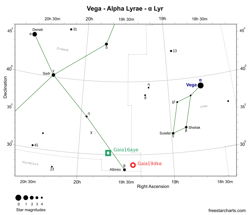
Figure 1: Location of the Gaia19dke event (red circle) is shown on the Cygnus - Lyra constellation map from www.freestarcharts.com. Also shown is the location of Gaia16aye binary microlensing (green square) event from Wyrzykowski et al. (2020).

Gaia DR3 for this object provides the following astrometric parameters:

$\varpi=(0.0718\pm 0.0267)$ mas, $\mu_{RA}=(-2.862\pm 0.022)$ mas/yr and $\mu_{\delta}=(-5.447\pm 0.029)$ mas/yr, where $\varpi$ is the stellar parallax of the source, and $\mu_{RA}$ and $\mu_{\delta}$ are proper motion components in right ascension and declination directions respectively measured at the reference epoch year 2016.

2.1 Gaia photometry

While Gaia scans the sky, it revisits the same location on average within 30 days. Each transit typically provides two independent measurements separated by 106 minutes coming from the two fields of view of the spacecraft (see Gaia Collaboration et al. 2016 for details). As of May 2023, Gaia has collected 191 measurements of Gaia19dke. The light curve from Gaia is collected in the Gaia broad-band filter $G$-band and exhibits multiple peaks, with the main peak reaching about 14.8 mag in August 2020.

A table with photometric data gathered by Gaia can be found in Table 6. GSA does not provide uncertainty on magnitudes in light curves for published events. We, therefore, used Gaia DR3 photometric time-series statistics (mean $G$-band magnitude and its standard deviation) to derive the mean expected uncertainties as a function of magnitude. The nominal error for the Gaia19dke magnitude range was computed as around 0.008 mag (Gaia Collaboration et al., 2018). Table 6 presents the uncertainty estimated for Gaia measurements, which were used throughout this work.

2.2 Ground-based photometric follow-up

Due to the fact that the event was relatively bright with $G\sim$15.5 mag at the baseline, it was possible to collect a vast number of follow-up observations using small-sized telescopes. The ground-based observations were carried out by a network of telescopes, including manually and robotically operated ones, listed in Table 4. To facilitate the coordination of observations and data processing, a web-based system called the Black Hole Target and Observation Manager (BHTOM) was utilized, which is based on LCO’s Target and Observation Manager TOM) Toolkit (Volgenau et al., 2022).

For each telescope, the acquired images underwent bias, dark, and flat calibration following each telescope’s procedures and the calibrated fits images were uploaded in near-real-time to BHTOM. PSF photometry was performed using CCDPhot (e.g. Zieliński et al. 2020; Rybicki et al. 2022, while standardization was achieved using the Cambridge Photometric Calibration Server (CPCS), as detailed in (Zieliński et al., 2019). Observations were conducted across various filters in both the SDSS and Johnson-Kron-Cousins systems. To establish uniformity, the data were standardized to the Gaia Synthetic Photometry (GaiaSP) catalogue (Gaia Collaboration et al., 2023a), with automated matching of instrumental data to the closest filter available in GaiaSP.

Table 5 lists the number of data points collected by each observatory, the time span of their data and the list of GaiaSP filters the observations were matched to. The table contains also the details on the data collected serendipitously for this target by the Zwicky Transient Factory (ZTF) Survey (Bellm et al., 2019) in $g$ and $r$ bands and provided by the IPAC service.

The earliest follow-up started 21 days after the announcement of the event on the GSA web page. The first data point was taken on the night of 29/30 August 2019, with the 60 cm telescope in the Astronomical Station Vidojevica (ASV) of Astronomical Observatory, Serbia. The follow-up then continued for over 2000 days until the event reached the baseline level again around May 2023. The data obtained by the follow-up network are available for download from BHTOM page for Gaia19dke (https://bhtom.space). In total, nearly 3000 data points were collected with the telescope network over a period of nearly 4 years.

2.3 Spectroscopic follow-up

In order to classify the object and to derive the properties of the source, Gaia19dke was also observed spectroscopically. The first spectrum was obtained close to the first brightness peak on December 11, 2019, with the Spectrograph for the Rapid Acquisition of Transients (SPRAT, Piascik et al. 2014) mounted on 2-m robotic Liverpool Telescope (LT, Steele et al. 2004) located in La Palma, Canary Islands, Spain. The spectrum was taken in the optical part of the electromagnetic window (400-800 nm) and low-resolution mode (R$\sim$350). It was reduced, and wavelength and flux were calibrated in a standard way by using an automated pipeline provided by the LT Team. The Xenon arc lamp was used to calibrate the spectrum in the wavelengths.

SPRAT data have shown the typical spectrum for normal G-type stars with prominent Mg 5167-5184 $\AA$ lines and Balmer series in absorption. No clear emission lines were registered, therefore, we do not observe any hints of stellar activity, variability, or the existence of circumstellar matter. Any of the features responsible for that was not registered in the SPRAT spectrum. Therefore, Gaia19dke was classified as a microlensing event candidate and further follow-up observations were planned.

The Microlensing Observing Platform automatically requested the spectroscopic monitoring for this target and a low-resolution spectrum (R$\sim$500) has been collected by the OMEGA collaboration on August 8, 2020 (the source was magnified by a factor 1.8 at this time, i.e. $G=14.9$ mag), with the FLOYDS instrument mounted on the Las Cumbres Observatory 2-m telescope at the Siding Spring observatory (Brown et al., 2013a). The spectrum has been reduced with the LCO FLOYDS pipeline. It confirmed the classification made based on SPRAT data showing absorption lines typical for a G-type star.

The low-resolution spectra of Gaia19dke gathered by SPRAT and FLOYDS instruments are presented together in Fig. 2.

Gaia19dke event reached a bright enough magnitude near its main peak around mid-2020 to be also observed with high-resolution spectroscopy. We used the Potsdam Echelle Polarimetric and Spectroscopic Instrument (PEPSI, Strassmeier et al., 2015) installed at the 2x8.4-m Large Binocular Telescope (LBT) located on Mt. Graham, Arizona, US. The data were taken on July 18, 2020, i.e., close to the maximum brightness of the event. The fibre diameter $300\leavevmode\nobreak\ \mu$m as well as two cross-dispersers (CD) were used: III (blue arm) and V (red arm) simultaneously. We were able to obtain a high-dispersion spectrum with an S/N ratio of around 31 and resolution R$\sim$43 000, which covers the wavelength range $383-907$ nm. It was calibrated by using the standard PEPSI software for stellar spectroscopy (SDS4PEPSI, (Ilyin, 2000)), i.e., images were bias subtracted, flat-fielded, and then optimally extracted and normalized using a spline fit to the continuum. Due to the poor quality of the spectrum below 480 nm, for further analysis, we used part above this threshold.

The spectrum from a high-resolution PEPSI spectrograph is presented in Fig. 3. In addition, the synthetic spectrum (red) generated based on the method described in Section 4 is over-plotted on the observed spectrum (blue).

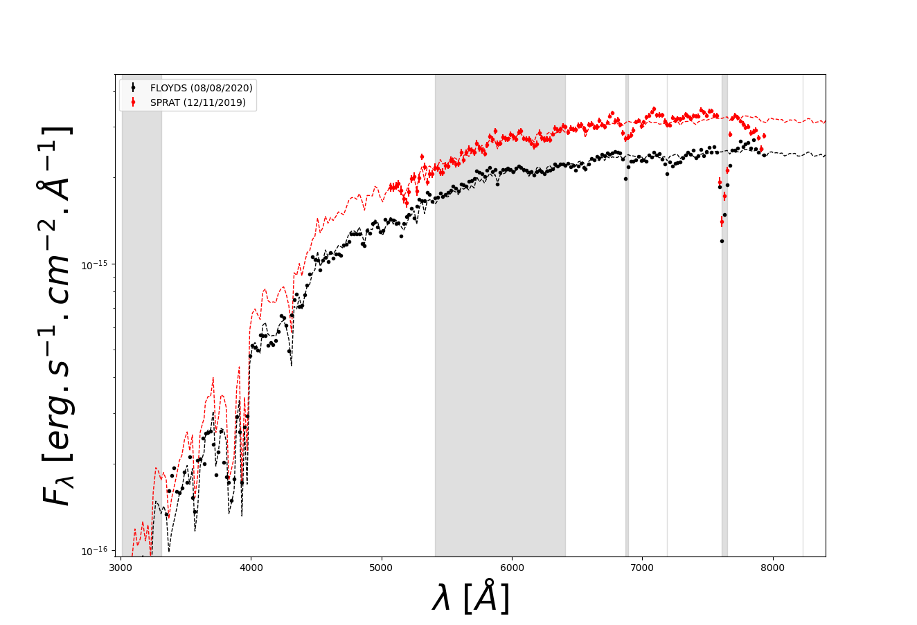
Figure 2: Low-resolution spectra of Gaia19dke obtained by LT/SPRAT (red points) and LCO/FLOYDS (black points) spectrographs. The grey parts of the plot denote the wavelength range with the telluric lines. The dashed lines correspond to the best-matching template spectra.

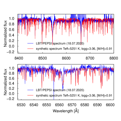
Figure 3: Spectrum of the Gaia19dke obtained on 18 July 2020 with LBT/PEPSI around the main peak of the event(blue) and the best-matching fit (red) synthesized for the specific parameters. The Ca II triplet (top) and H$\alpha$ (bottom) region are presented.

2.4 High-resolution imaging follow-up

Gaia19dke was observed with the Gemini North 8-m telescope using the ‘Alopeke speckle imaging instrument on 9 August 2020. ‘Alopeke is a simultaneous two-channel EMCCD instrument that performs speckle interferometric imaging. Using narrow-band filters centred at 562 nm and 832 nm, the images are obtained with 60 msec integration times and collected in sets of 1000 such images/set. The final product from ‘Alopeke imaging is a high-resolution image in each filter with an inner working angle at the diffraction limit, near 20 mas for the 8-m Gemini telescope, and covering a small field of view out to 1.2 arcsecs.

The set of images was subjected to Fourier analysis in our standard reduction pipeline (Howell et al., 2011). Figure 4 shows the final 5-$\sigma$ contrast curves in each filter and the 832 nm reconstructed speckle image. We find that the object at Gaia19dke is not resolved beyond a single point source, even down to the 20 mas inner working angle.

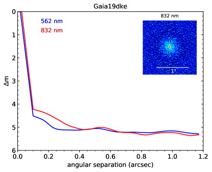
Figure 4: Contrast curves for red and blue narrow-band filters obtained from speckle interferometric observations of Gaia19dke obtained on 2020 Aug.9 with ’Alopeke instrument at the Gemini telescope. The inset shows the combined set of images in an 832 nm filter.

3 Photometric Microlensing Model

The photometric data of Gaia19dke has been modelled with the single point source single lens microlensing model with annual parallax(e.g. Gould, 2000; Smith et al., 2002; Wyrzykowski et al., 2016; Rybicki et al., 2022; Kruszyńska et al., 2021). We used open-source flexible software MulensModel(Poleski & Yee, 2019) for finding the model parameters.

The parallax model is described with the following parameters:

• $t_{0}$, time of the minimal approach between the lens and the source;

• $u_{0}$, impact parameter, the minimal distance between the lens and the source in units of the Einstein Radius;

• $t_{E}$, the time-scale of the event, defined as the time to cross the Einstein Radius;

• $\@vec{\pi_{E}}$, vector of the microlensing parallax, decomposed into equatorial North $\pi_{EN}$ and East $\pi_{EE}$ components;

• $mag_{0}$, baseline magnitude(s), separately in each observing band, computed in MulensModel from source flux;

• $f_{S}$, blending parameter(s), separately in each observing band, defines as the flux of the source over the total baseline flux, composed of source and blend(s) and/or lens light, computed in MulensModel from source and blend fluxes;

The microlensing parallax model has been fitted in a geocentric frame with a fixed $t_{0_{par}}$ parameter, set to the time of the maximum of the light curve, hence very close to $t_{0}$. To find the most likely model, we used Markov chain Monte Carlo (MCMC) implemented in the emcee package (Foreman-Mackey et al., 2013). Since Gaia observed Gaia19dke from L2 point, we included the space-parallax factor in MulensModel.

We used all photometric light curve data gathered by the end of May 2023, when the event reached its baseline magnitude. We first modelled Gaia data only, as it covers the shape of the event densely and contains a couple of years of the baseline prior to the microlensing event. Table 1 contains the values of microlensing model parameters found when fitting Gaia-only data. Our procedure identified only one solution in the parameter space for negative $u_{0}$. Figure 5 shows the Gaia photometric data together with the best microlensing model with a parallax fit to that data.

Subsequently, the microlensing model fitting was performed using the combined dataset of Gaia observations, follow-up observations, and data from the Zwicky Transient Facility (ZTF). Given that all observations, acquired with a network of telescopes, underwent consistent calibration and standardization to GaiaSP bands, we were able to effectively utilize the entire collected dataset from all telescopes, a total of nearly 5000 data points. However, we excluded 30 points calibrated to $u$, $U$, and $z$ filters, as they were erroneously matched to incorrect bands and exhibited clear outliers. The modelling has been carried out in each GaiaSP band separately.

Table 1 shows the values of microlensing model parameters found for Gaia and the follow-up data set combined. The baseline magnitude and blending parameters were found separately for each observatory and filter. There was also only one parallax solution found for this data set. Figure 6 shows the best microlensing model and its residuals fitting the Gaia and follow-up observations.

The parameters obtained in the two models agree within the margin of error, but the model constructed using follow-up photometric observations exhibits narrower error bars, a factor of 3 to 5 better, which translates to more precise parameter estimates and improved accuracy. In order to achieve more continuous samples from the parameter space, in the modelling process we allowed the blending parameter $f_{s}$ to be greater than one. Samples with $f_{s}$ greater than one should be treated as if there is no blending at all. In both models, the value of the blending parameter is very close to 1, in particular, for ${\it{Gaia}}$ band, $f_{s}=1$ within the margin of error. Other bands yielded slightly lower values of $f_{s}$ (e.g. I(GaiaSP)), which can be attributed to low spatial resolution of instruments collecting these data and the observed blending is caused by nearby stars falling within their disks of Point Spread Function.

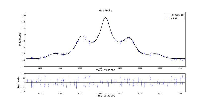
Figure 5: Light curve of Gaia19dke microlensing event with data only from Gaia, spanning from JD = 2458062 to JD = 2460062. The black line is the mode of the chains from the MCMC model. The bottom panel shows the residuals with respect to the mode solution.

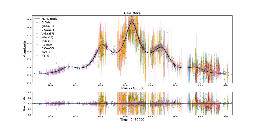
Figure 6: Light curve of Gaia19dke microlensing event with data from Gaia and follow-up observations, spanning from JD = 2458062 to JD = 2460062. Black line is the mode of the chains from the MCMC model. The bottom panel shows the residuals with respect to the mode solution.

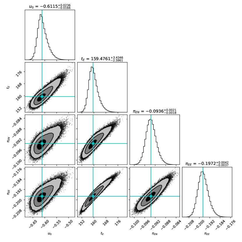
Figure 7: Chi-squared contours plotted as a function of the parameters fitted in the MCMC fit for the best model for the Gaia19dke event obtained with Gaia-only data. Black, dark grey and light grey solid colours represent $1\sigma$, $2\sigma$, and $3\sigma$ confidence regions respectively. Black dots represent solutions outside of the $3/sigma$ confidence level. Cyan lines and squares mark the median solution reported in Table 1. The plot has been created using corner python package by Foreman-Mackey (2016).

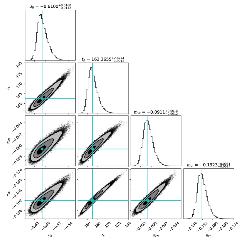
Figure 8: Chi-squared contours plotted as a function of the parameters fitted in the MCMC fit for the best model for the Gaia19dke event obtained after including the follow-up data. Black, dark grey and light grey solid colours represent $1\sigma$, $2\sigma$, and $3\sigma$ confidence regions respectively. Black dots represent solutions outside of the $3\sigma$ confidence level. Cyan lines and squares mark the median solution reported in Table 1. The plot has been created using corner python package by Foreman-Mackey (2016).

Table 1: Microlensing parallax model for Gaia-only data and Gaia with follow-up observations.

Parameter	Gaia-only	Gaia+FUP
$t_{0,par}-2450000.$ [JD]	-	9068
$t_{0}-2450000.$ [JD]	9065.39${}^{+0.82}_{-0.81}$	9064.0639${}^{+0.33}_{-0.33}$
$t_{\mathrm{E}}$	159.48${}^{+3.43}_{-2.60}$	162.47${}^{+2.68}_{-1.90}$
$u_{0}$	-0.6115${}^{+0.0236}_{-0.0166}$	-0.6100${}^{+0.0160}_{-0.0112}$
$\pi_{\mathrm{EN}}$	-0.0936${}^{+0.0021}_{-0.0018}$	-0.0911${}^{+0.0014}_{-0.0012}$
$\pi_{\mathrm{EE}}$	-0.1972${}^{+0.0042}_{-0.0037}$	-0.1923${}^{+0.0031}_{-0.0024}$
$mag_{0}$ $G$ (Gaia)	15.5052${}^{+0.0007}_{-0.0006}$	15.5059${}^{+0.0005}_{-0.0004}$
$f_{\mathrm{S}}$ $G$ (Gaia)	1.0045${}^{+0.0437}_{-0.0604}$	0.9947${}^{+0.0301}_{-0.0421}$
$mag_{0}$ $B$(GaiaSP)	-	17.2458${}^{+0.0007}_{-0.0006}$
$f_{\mathrm{S}}$ $B$(GaiaSP)	-	0.9162${}^{+0.0280}_{-0.0397}$
$mag_{0}$ $g$(GaiaSP)	-	16.6105${}^{+0.0014}_{-0.0014}$
$f_{\mathrm{S}}$ $g$(GaiaSP)	-	0.9832${}^{+0.0303}_{-0.0426}$
$mag_{0}$ $i$(GaiaSP)	-	14.9657${}^{+0.0298}_{-0.0419}$
$f_{\mathrm{S}}$ $i$(GaiaSP)	-	0.9685${}^{+0.0298}_{-0.0419}$
$mag_{0}$ $I$(GaiaSP)	-	14.4646${}^{+0.0008}_{-0.0007}$
$f_{\mathrm{S}}$ $I$(GaiaSP)	-	0.8624${}^{+0.0265}_{-0.0375}$
$mag_{0}$ $r$(GaiaSP)	-	15.4483${}^{+0.0010}_{-0.0010}$
$f_{\mathrm{S}}$ $r$(GaiaSP)	-	0.9324${}^{+0.0289}_{-0.0409}$
$mag_{0}$ $R$(GaiaSP)	-	15.2199${}^{+0.0007}_{-0.0007}$
$f_{\mathrm{S}}$ $R$(GaiaSP)	-	0.9849${}^{+0.0301}_{-0.0427}$
$mag_{0}$ $V$(GaiaSP)	-	15.9731${}^{+0.0007}_{-0.0007}$
$f_{\mathrm{S}}$ $V$(GaiaSP)	-	0.9987${}^{+0.0306}_{-0.0433}$
$mag_{0}$ $g$(ZTF)	-	16.5351${}^{+0.0009}_{-0.0009}$
$f_{\mathrm{S}}$ $g$(ZTF)	-	0.9690${}^{+0.0297}_{-0.0421}$
$mag_{0}$ $r$(ZTF)	-	15.3947${}^{+0.0009}_{-0.0008}$
$f_{\mathrm{S}}$ $r$(ZTF)	-	0.9777${}^{+0.0290}_{-0.0404}$
$\chi^{2}$	556.7	3621.64

4 Source star

In order to determine the parameters of the lensing object, the initial step involves deducing the distance and the spectral type of the source star.

Our study is based on the assumption that the source star is single since there are no signs of its binarity in the microlensing model. Moreover, according to Gaia EDR3, the closest object is 1.6 arcsecs away and is significantly fainter.

4.1 Atmospheric parameters

The parameters of the source star in the Gaia19dke event were derived from spectroscopic follow-up datasets, high-resolution data obtained with LBT/PEPSI and low-resolution data from two instruments: LT/SPRAT and LCO/FLOYDS.

The spectroscopic analysis of absorption lines visible in high-resolution PEPSI spectrum was performed first. We used iSpec framework for spectral analysis which integrates several well-known radiative transfer codes (Blanco-Cuaresma et al., 2014; Blanco-Cuaresma, 2019). In our case, to determine atmospheric parameters (i.e., effective temperature $T_{\rm eff}$, surface gravity $\log g$, metallicity [M/H], microturbulence velocity $v_{\rm t}$), the SPECTRUM code was used. We generated a set of synthetic spectra based on a well-known grid of MARCS atmospheric models (Gustafsson et al., 2008) and solar abundances taken from Grevesse et al. (2007). The synthetic spectra were fitted to the observational spectrum for selected regions containing H$\alpha$, Ca, Mg, Fe, Na, and Ti atomic lines. The best-matching solution was found for the following parameters: $T_{\rm eff}=(5251\pm 25)$ K, $\log g=(3.06\pm 0.02)$, $\mathrm{[M/H]}=(0.91\pm 0.03)$ dex and $v_{\rm t}=(1.23\pm 0.07)$ km s^-1. According to these parameters, we assume that our source star is a metal-rich G5-type giant. Moreover, no absorption lines from a potential second component are visible in PEPSI data. Fig. 3 shows the result of this analysis, i.e., PEPSI spectrum and synthetic fit for Ca II triplet and H$\alpha$ region are presented.

After that, we modelled the spectroscopic data with templates on the full wavelength range. This approach is complementary to the analysis of absorption lines presented above. Following the method of Bachelet et al. (2022), we fitted the FLOYDS and SPRAT spectra with templates from (Kurucz, 1993) with the Spyctres pipeline. The new version of Spyctres includes the updated extinction law from Cardelli et al. (1989a) to the one of Wang & Chen (2019). In short, the latter combines an adjustment of the Cardelli et al. (1989a) law with a fixed total-to-selective extinction ratio $R_{V}=A_{V}/E(B-V)=3.1$ and a power-law index $\alpha=2.07$ for the near-IR regions. The data and results are presented in the Fig. 2. The template-matching analysis reveals that the source is a red giant, with an effective temperature $T_{eff}=(5000\pm 200)$ K, a sun-like metallicity $[M/H]=(0.0\pm 0.3)$ dex, a surface gravity $\log g=(2.2\pm 0.5)$, an angular radius $\theta_{*}=(7.9\pm 0.4)\leavevmode\nobreak\ \mu as$ and an absorption $A_{v}=(1.6\pm 0.2)$ mag.

The results obtained from absorption line analysis and template-matching are in good agreement, except the metallicity, and are presented in Tab. 2.

Table 2: Summary of the derived parameters for the source of Gaia19dke event. Averaged solutions of line fitting and template matching are presented.

Parameter	Line fitting	Template Matching
$T_{\rm eff}$ [K]	$5251\pm 25$	$5000\pm 200$
${\log g}$	$3.06\pm 0.02$	$2.2\pm 0.5$
${\rm[M/H]}$ [dex]	$0.91\pm 0.03$	$0.0\pm 0.3$
$v_{\rm t}$ [km/s]	$1.23\pm 0.07$	–
$A_{\rm v}$ [mag]	–	$1.6\pm 0.2$
${\rm\theta_{*}}$ $[\mu as]$	–	$7.9\pm 0.4$

4.2 Source distance

One of the simplest and most popular ways to determine the distance to the star is to use the Bailer-Jones et al. (2021) catalogue, where distances were calculated based on the Gaia EDR3 and priors on the Galaxy. Geometric distance, based on the parallax and its uncertainties, gives the distance to Gaia19dke source star of $7.6<D_{s}<11.9$ kpc. The photo-geometric value, which is based on the parallax, the colour as well as the observed magnitude of the star, gives the distance of $6.7<D_{s}<9.2$ kpc. We note here, that the values based on Gaia parallax measurement in case of microlensing events should be considered with great care, as the parallax measurement can be affected by the light of the lens, if luminous, or any other blends in the line of sight. Moreover, if the parallax measurement obtained from the astrometric time-series collected at the time of the event, the astrometric data can be also affected by the astrometric microlensing effect (e.g. Rybicki et al. 2018; Sahu et al. 2022; Jabłońska et al. 2022). Therefore, in order to verify the distance to the source star, we use the spectroscopic data and apply the well-known spectro-photometric equation:

$$5\log D_{S}=V-M_{V}+5-A_{V},$$ (3)

where $D_{S}$ is the distance to source star, $V$ is the apparent magnitude, $M_{V}$ is the absolute magnitude and $A_{V}$ is the interstellar extinction.

In the present work, we used the atmospheric parameters based on the high-resolution PEPSI spectrum where the star is classified as G5 giant, while the extinction value $A_{V}=1.6\pm 0.2$ mag was taken from the template matching analysis of low-resolution spectra.

The typical absolute magnitude and error for G5 giant star are $M_{V}=(1.0\pm 0.5)$ mag (Straižys, 1992). Together with the apparent magnitude of Gaia19dke $V=16.101$ mag (Stassun et al., 2019) and accepting extinction value $A_{V}=1.6$ mag determined from the low-resolution spectra and taking into account the non-linearity of the transformation and asymmetry of the distance, $\log_{10}(D_{S})$, we have determined the distance to the source star of Gaia19dke $D_{s}=(4.9\pm 1.2)$ kpc which is a factor of two different from Bailer-Jones et al. (2021)’s values. It is in good agreement with the template matching analysis that points towards a source distance of $D_{s}=4.3^{+3.3}_{-1.1}$ kpc assuming a source age of 1 Gyr and using the isochrones from Bressan et al. (2012) and Marigo et al. (2013).

Because of the significant difference between our spectroscopic distance and literature values from Bailer-Jones et al. (2021), we should critically evaluate which value is the most real and which one should be used for determining the lens parameters.

To independently verify the source star parameters we apply other available methods based on accessible databases. We used infrared photometry from 2MASS (Skrutskie et al., 2006) survey were source stars measured magnitudes in $J=(13.348\pm 0.024)$ mag, $H=(12.766\pm 0.024)$ mag and $K_{s}=(12.550\pm 0.023)$ mag. According to (Straižys & Lazauskaitė, 2009), the intrinsic colour of the G5 giant star should be $(J-K_{s})_{0}=0.49$ mag.

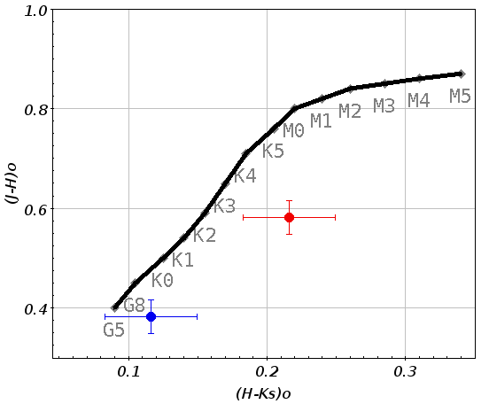
Figure 9: Colour-colour $(J-H)_{0}$ vs. $(H-K)_{0}$ diagram for the intrinsic red giant’s branch (black line). Spectral classes, corresponding to the intrinsic colours, are indicated close to the line. The value for Gaia19dke is plotted as a red point with errors. De-reddened and shifted according to an extinction value $A_{K_{s}}=0.21$ mag is shown as a blue point with errors.

For the source star, the colour excess and interstellar extinction were calculated with the following equations (Dutra et al., 2002):

$$E_{J-K_{S}}=(J-K_{s})_{\rm obs}-(J-K_{s})_{0},\\ A_{K_{s}}=0.67\,E_{J-K_{S}},$$ (4)

where $E_{J-K_{S}}$ is the colour excess, $(J-K_{s})_{\rm obs}$ is the observed colour, $(J-K_{s})_{0}$ is the the intrinsic colour, and $A_{K_{s}}$ is the interstellar extinction in $K_{s}$ band.

According to Eq. 4, the estimated extinction value for this star is $A_{K_{s}}=0.21$ mag. The extinction value $A_{K_{s}}$ transformed to the $A_{V}$ with the following relation (Cardelli et al., 1989b; Dutra et al., 2002):

$$A_{V}=8.3A_{K_{s}},$$ (5)

The estimated value of $A_{V}=1.7\pm 0.3$ mag is in excellent agreement with the value determined by template-matching based on low-resolution spectra $A_{V}=1.6\pm 0.2$ mag. Fig. 9 shows the location of the source star in the 2MASS $(J-H)_{0}$ vs. $(H-K)_{0}$ diagram for the observed and dereddened according to an extinction value. The intrinsic red giant’s branch is shown as a black line. The dereddened star position on the diagram shows acceptable agreement with extinction and spectral class determined based on low- and high-resolution spectra collected for Gaia19dke.

We used another method that allows us to verify extinction was proposed by (Majewski et al., 2011) based on combined 2MASS and Spitzer colour indices $H$-[4.5], since for most of F-G-K stars are close to the zero. Here [4.5] is the magnitude at 4.5 $\mu$m of the Spitzer IRAC system. We have to apply the WISE (Wright et al., 2010) system since the Spitzer measurements are absent and taking into account that WISE $W2$ measurements with the 4.6 $\mu$m mean wavelength direct comparison (Jarrett et al., 2011) shows little scattering. Using WISE measured magnitude $W2=(12.524\pm 0.027)$ mag, for the source star, interstellar extinction was calculated with the equation:

$$A_{K_{s}}=0.918\,(H-W2-0.08),$$ (6)

In this way, the estimated extinction value $A_{K_{s}}=0.149$ mag is by 0.06 mag smaller than previously determined using only 2MASS.

The answer seems obvious that extinction value $A_{V}=1.6$ mag determined by the spectroscopic analysis and compared with different methods matches with calculated using different databases.

For distance check, we also use 2MASS photometry. We again apply the spectro-photometric method but use 2MASS $K_{s}$ where distance is determined with the following equation:

$$5\log D_{S}=K_{s}-M_{K_{s}}+5-A_{K_{s}},$$ (7)

The most uncertain in Eq.7 are $M_{K_{s}}$ for the type G5 giants. We assume its value of $-1.5$ mag since the location in $M_{K_{s}}$/$J-K$ HR diagram is on the left edge from the Red Clump Giant (RCG) position (Veltz et al., 2008). We do not exclude that the real $M_{K_{s}}$ may vary more than $\pm 0.5$ mag. Using 2MASS photometry we just verify the distance and we determine $D_{s}=(6.0\pm 1.4)$ kpc to the source star.

As demonstrated above, spectro-photometric method based on optical and infrared data yielded a similar value in the source distance as the one using spectra. We assume that the optically determined distance is more reliable than the infrared one because, in the 2MASS colour-colour diagram, the star only coincides with the actual position of the G5 giant within the error limits, which can be explained by the measurement errors. We can not exclude some variability properties (Henry et al., 2000) since it can change observed magnitude and colour, consequently and source star location on 2MASS colour-colour diagram.

Throughout the work, we, therefore, use the source distance determined with the PEPSI spectrum, $D_{s}=(4.9\pm 1.2)$ kpc.

5 Lensing object

The microlensing model found for Gaia19dke (Section 3) indicates no additional light in the event apart from the source. This is encompassed in the blending parameters derived for each photometric band, as listed in Table 1. Blending can originate from both the lens itself as well as any star located in close vicinity of the event and unresolved by the photometry. Gaia19dke is located in the Galactic Disk, where the stellar density is significantly lower than in typical microlensing fields in the Galactic Bulge, hence we do not expect any additional source of light close to it, which is confirmed with the high-angular resolution imaging with ’Alopeke (Sec.2.4).

In order to constrain the nature of this dark lensing object, hence its mass and distance, we adopted the method outlined in (Wyrzykowski et al., 2016), (Mróz & Wyrzykowski, 2021), (Kruszyńska et al., 2021), (Kaczmarek et al., 2022) and explained in detail in Howil et al. (in prep.). The microlensing parameters and their samples from MCMC obtained in previous steps, described in Section 3, were combined with priors on the mass, distance, and velocity distribution of stars in the Galaxy for the lens and the source. Blending parameters $f_{\mathrm{S}}$ of for both Gaia-only and Gaia with follow-up are close to 1, which means Gaia registers the movement and position of the source star. We have thus adopted the proper motion for the source star as published in Gaia EDR3. For the distance, we used the value obtained from spectral analysis, described in Section 4. In each iteration, we have drawn from a Gaussian distribution of distances with a mean of $4.9\,\text{kpc}$ and a spread of $1.2\,\text{kpc}$. This method requires also knowing the value of the extinction $A_{\mathrm{G}}$ towards the lens, to constrain the light coming from the lens if it was an MS star. We used the value presented in Gaia DR2 catalogue, which lists $A_{\mathrm{G}}$ under a_g_val in gaia_source table and is equal to $A_{\mathrm{G}}=0.8043$ mag. We assume this value to be the maximal possible extinction in the direction towards the lens. Finally, we had to assume the relative proper motion of the lens and source $\mu_{\mathrm{rel}}$. For this, we drew a random number between 0 and 30 mas $\mathrm{year}^{-1}$ (Mróz & Wyrzykowski, 2021). This allowed us to find the distance and mass to the lens in combination with the $\pi_{\mathrm{E}}$ and $t_{\mathrm{E}}$ obtained from the posterior distribution of parameters of the best-fitting microlensing model solution and the distance mentioned above to the source. Knowing the mass and distance of the lens, we could derive the observable brightness of the lens as if it was the MS star using empirical data from Pecaut & Mamajek (2013) and compare it to the constraints on the brightness of the lens we obtained from microlensing model. We then computed a weight using a set of priors from Skowron et al. (2011) for all the pairs of lens mass $M_{\mathrm{L}}$ and lens distance $D_{\mathrm{L}}$. For the mass function prior we used the value of -2.35, following the classical mass function for stars (Kroupa & Weidner, 2003).

The results of this analysis are shown in Figures 10 and 11. The histograms of the distribution of the lens mass and lens distance are visible in Figures 12 and 13. Table 3 contains the summary of the median values of the mass, distance, blend light, and lens light in the case of an MS star lens. For Gaia-only data model the median mass is $M_{\mathrm{L}}=0.50^{+3.01}_{-0.40}\leavevmode\nobreak\ M_{\odot}$ and distance $D_{\mathrm{L}}=3.08^{4.09}_{-2.45}$ kpc. For combined Gaia and follow-up data, the median mass and distance are $M_{\mathrm{L}}=0.51^{+3.07}_{-0.40}\leavevmode\nobreak\ M_{\odot}$ and $D_{\mathrm{L}}=3.05^{+4.10}_{-2.42}$ kpc, respectively. Modes of the distributions are, respectively, $M_{\mathrm{L}}=0.27\leavevmode\nobreak\ M_{\odot}$, $D_{\mathrm{L}}=2.31$ kpc, for G model and $M_{\mathrm{L}}=0.28\leavevmode\nobreak\ M_{\odot}$, $D_{\mathrm{L}}=2.26$ kpc, for G+F model.

Figure 11 contains the comparison of the light of the blend obtained from the microlensing model and the light of the lens if the lens is the MS star. Lines divide the plot area into two cases: above both lines prevail the scenario where the MS is justified given the blending. Below the lines, the light of the lens as an MS star is greater than the actual light of the lens we get from the microlensing model, suggesting a dark lens scenario. The solid line denotes the scenario, when the value of the extinction is equal to the one for the source, while the dashed line assumes no extinction to the lens at all. The luminous lens dark-lens scenario is preferred with 57% to 63% probability (for Gaia-only solution) and 58% to 64% for G+F model, with the range of probabilities resulting from a range of possible extinction values to the lens.

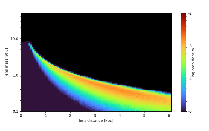
Figure 10: Dark Lens code output for Gaia19dke microlensing solution. Lens mass-distance probability density.

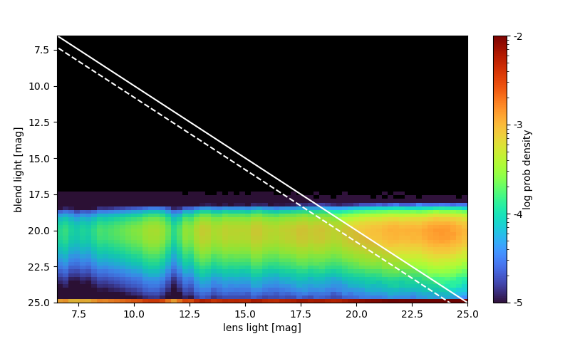
Figure 11: Dark Lens code output for Gaia19dke microlensing solution. G-band blend light vs lens light probability density. The lines divide between the case where the lens was more luminous than the total blended light. The dashed line is for no extinction to the lens, while the solid line is for the assumption that the lens is behind the same extinction as the source. Negative blending samples are shown artificially at blend light=25mag.

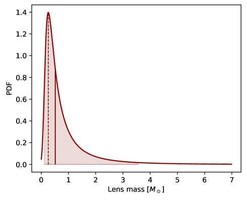
Figure 12: Probability density plot for the mass of the lens for G+F solution. The solid line marks the median and the dashed line marks the mode. The filled red area represents the $95\%$ confidence interval.

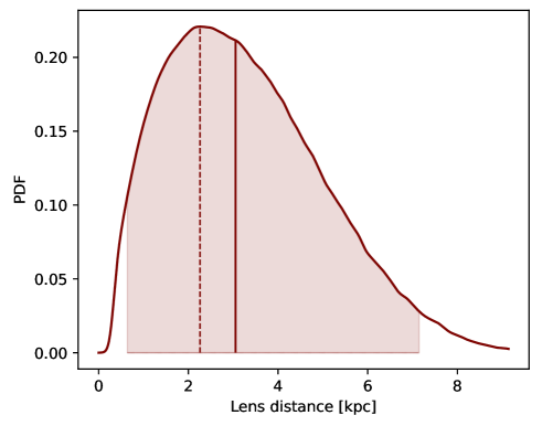
Figure 13: Probability density plot for distance to the lens for G+F solution. The solid line marks the median, and the dashed line marks the mode. The filled red area represents the $95\%$ confidence interval.

Table 3: Lens masses $M_{\mathrm{L}}$, distances $D_{\mathrm{L}}$ and size of the Einstein Radius $\theta_{E}$ for the microlensing solutions.

Parameter	G	G+F
$G_{bl}$ [mag]	$ND$	$>22.6$
$M_{\mathrm{L}}$ [$M_{\odot}$]	$0.50^{+3.01}_{-0.40}$	$0.51^{+3.07}_{-0.40}$
$D_{\mathrm{L}}$ [kpc]	$3.08^{+4.09}_{-2.45}$	$3.05^{+4.10}_{-2.42}$
$\theta_{E}$ [mas]	$0.87^{+5.35}_{-0.68}$	$0.90^{+5.37}_{-0.70}$
Prob(DL)	57.2%-63.4%	58.4%-64.5%
$\mathrm{SpT}_{\mathrm{MS}}$	M1V	M1V
$G_{\mathrm{MS}}$[mag]	22.1-21.3	22.1-21.3

6 Discussion

The microlensing event Gaia19dke lasted for about 2000 days (more than 5 years), making it one of the longest events ever studied. The annual parallax due to Earth’s orbital motion caused a very strong microlensing parallax anomaly to a standard Paczynski curve visible in the light curve as a series of multiple peaks(Smith et al., 2002). Typically in parallax events, the $u_{0}$ sign and $\pi_{E}$ (N-E) degeneracy are present, in particular, this is common in the case of Bulge events, where the Ecliptic crosses the Galactic Plane. In Gaia19dke, located at about 300,50 deg in ecliptic coordinates, there was only one unique solution found for microlensing parallax. The annual parallax is measurable from Gaia data alone. However, adding the extensive ground-based follow-up observations improves the parallax vector measurement by a factor of 3. The space-based parallax between Gaia and the ground-based observatories was included in the model, however, was too small to be detected.

The microlensing parameters measured based solely on photometric Gaia data were derived with an accuracy of about 1-3%. The addition of extensive ground-based follow-up observations improved the determination of all parameters by a factor of about 3. In particular, the improvement is the strongest in the case of the impact parameter $u_{0}$ and Einstein time-scale $t_{E}$, while the uncertainty on the parallax vector is about 0.8% with the follow-up data.

More importantly, the blending parameter for ${\it{Gaia}}$ data has been determined more accurately when including follow-up data, from 4% to around 1%, which additionally supports the dark-lens case scenario. Blending parameters determined for all other modelled bands additionally confirm there is no or very little extra light apart from the source, with values of the blending very close to 1. Combining this information with no detection of any additional sources in the high-resolution image from ’Alopeke, strengthens the dark or very faint lens case. We decided to use ${\it{Gaia}}$’s blending parameter in the lens nature determination in Section 5 because GSA data covers both sides of the light curve, both its rising and declining parts as well as the baseline before the event, while other data sets covered only the central part of the event.

Microlensing in Gaia19dke allows us to determine the lens mass and its distance only because we measure the microlensing parallax and we use the priors on the lens proper motions as well as its distance and slope of the mass function. The results for mass and distance of the lens are summarised in Table 3, however, it should be noted that all the resulting posterior distributions are non-symmetric. Nevertheless, when using median values for mass and distance for either solution, we find the lens would need to be an M1V spectral-type star if it was a main sequence object. Placed at a median distance it would shine at 21.3 mag or 22.1 mag if all extinction measured to the source was in front of the lens. When compared with the amount of blending we measure in the light curve and its microlensing model, we can rule out such a scenario of a luminous lens. For a more massive lens, its distance would be even shorter, yielding an increase in the brightness of the alleged main sequence star. Only masses lower than the median would be possible to be explained within the observed bounds for blended light. The total integral over the parameter space yields between 57 and 64% dark lens probability for both G and G+F models, the range resulting from including none or all extinction to the lens light.

The high angular-resolution image obtained on 2020 Aug.9 with ’Alopeke instrument at the Gemini telescope does not show any visible additional object within 20 mas. From the long-term microlensing light curve analysis which started on the 8th of August 2019 and involved a massive ground telescope follow-up campaign that allowed us to collect a very detailed light curve for Gaia19dke, we also did not detect any binary lens signatures, typically visible as deviations to standard lensing curve and sharp caustic crossings. This strengthens the explanation of the shape of the light curve as microlensing by a single lens, affected by the parallax effect due to the Earth’s orbit. We, therefore, suggest the lensing event could have been caused by a stellar remnant.

Stellar evolution theory predicts that White Dwarfs (WDs) are the most common stellar remnants in the Galaxy. However, it is important to notice that, because of low brightness, the detection of WD is challenging. The majority of known WDs were found within the around 100 pc Gentile Fusillo et al. (2019), consequently, a full understanding of the WD population is far from complete. According to Takahashi et al. (2013) the upper mass limit for a WD is 1.367 $M_{\odot}$, confirmed with the recent discovery of 1.35 $M_{\odot}$ WD (Caiazzo et al., 2021). The most common mass of WD, however, falls within the range of $0.6M_{\odot}$ - $0.7M_{\odot}$ (McCleery et al., 2020).

The most probable mass of the lens in our models is around 0.5 $M_{\odot}$, making the WD option most feasible. However, the possible mass range for the lens (Fig. 12) also spans to larger masses, hence we can not rule out even a nearby neutron star scenario.

Gaia19dke event is an excellent example of microlensing events for which ${\it{Gaia}}$’s astrometric time-series will provide an actual measurement of the lens mass and distance through measurement of a tiny displacement of the source star due to microlensing (Dominik & Sahu, 2000; Belokurov & Evans, 2002). In the case of non-blended events like this one, the shift in the position of the source is of the order of the size of the Einstein Radius. Using Galaxy priors we estimate this size to be about 1 mas, hence easily detectable in the ${\it{Gaia}}$ astrometric data (Rybicki et al., 2018; Jabłońska et al., 2022; Wyrzykowski et al., 2023).

7 Conclusions

In this work, we presented the investigation and analysis of a very long multi-peak microlensing event Gaia19dke located in the Galactic Disk, discovered by the Gaia space satellite. The event exhibited a microlensing parallax effect perturbed by the Earth’s orbital motion. The investigation is based on Gaia data and ground follow-up photometry and spectroscopy follow–up observations. We determined the source star distance to $D_{S}=(4.9\pm 1.2)$ kpc and we estimated the lens mass of $M_{L}=(0.50^{+3.07}_{-0.40})M_{\odot}$ and its distance of $D_{L}=(3.05^{+4.10}_{-2.42})$ kpc for the model including both ${\it{Gaia}}$ and ground-based data. Since essentially all of the detected light is coming from the source, a possible explanation is that the lens is a dark remnant candidate, most likely a single WD star, but a neutron star can also be considered.

The conclusive answer to the question on the nature of the lens will come with the ${\it{Gaia}}$ astrometric time-series data to be released within DR4 (part until mid-2019) and DR5 (all remaining data). Additionally, the high-resolution AO-assisted observations of the source star in about a decade should provide strong confirmation on the dark lens in case of a non-detection of the lens(e.g. Blackman et al., 2021).

8 Appendix

8.1 Photometry

Here we present the photometric data used for modelling Gaia19dke.

Table 4: Telescopes involved in the photometric follow-up observations of Gaia19dke

Observatory	Name	Location	Longitude	Latitude	Ref.
			[deg] (E+)	[deg]
ASV	1.4-m Milankovic Telescope	Vidojevica, Serbia	21.56	43.14	1
	60-cm Nedeljkovic Telescope	Vidojevica, Serbia	21.56	43.14	1
	Astronomical Observatory of Belgrade
Abastumani	36-cm telescope	Mount Kanobili,	42.82	41.75	2
	Georgian National Astrophysical Observatory	Georgia
Adiyaman 60	60-cm telescope	Adiyaman, Turkey	41.23	39.78	3
	Adiyaman University Observatory
Adonis	25-cm Adonis Observatory telescope	Langemark, Belgium	2.93	50.92	-
Astrolab	68-cm NMPT telescope	Ypres, Belgium	2.91	50.82	4
	Astrolab IRIS Observatory
Białków	60-cm Cassegrain telescope, Białków Observatory	Białków, Poland	16.66	51.48	5
	Astronomical Institute, University of Wrocław
Flarestar	25-cm Schmidt-Cassegrain telescope	San Gwann,	14.47	35.90	6
	Flarestar Observatory	Malta
HAO	68-cm Horten telescope	Nykirke, Norway	10.39	59.43	-
IST60	60-cm Ritchey-Chretien telescope	Ulupinar, Turkey	26.47	40.10	7
Krakow CDK500	50-cm telescope	Kraków, Poland	19.83	50.05	8
	Astronomical Observatory of the Jagiellonian University
LCO 1m	1.0-m telescope	Texas, US	-104.02	30.67	9
	McDonald Observatory
LCO 1m	1.0-m telescope	Izaña, Tenerife	-16.51	28.30	9
	Tenerife Observatory	Spain
Loiano	1.52-m Cassini Telescope,	Bologna, Loiano, Italy	11.33	44.26	10
	Bologna Observatory of Astrophysics and Space Science
Moletai35	35-cm Maksutov telescope,	Molėtai, Kulionys,	25.56	55.32	11
	Molėtai Astronomical Observatory	Lithuania
Ostrowik60	60-cm Cassegrain telescope,	Ostrowik, Poland	21.42	52.09	12
	Warsaw University Astronomical Observatory
Piwnice 90	90-cm Schmidt-Cassegrain telescope	Piwnice, Poland	18.56	53.09	13
	Institute of Astronomy, Nicolaus Copernicus University
RBT	70-cm CDK telescope, Adam Mickiewicz University	Winer Observatory, AZ, USA	-110.60	31.66	24
Rozhen60	60-cm Cassegrain telescope	Rozhen, Bulgaria	24.74	41.7	14
	Rozhen National Astronomical Observatory
RRRT	60-cm Rapid Response Robotic Telescope	Virginia, US	-78.69	37.88	15
	Fan Mountain Observatory
SUTO-Otivar	30-cm Newtonian telescope	Otivar, Spain	-3.68	36.82	16
	Silesian University of Technology Observatory
SUTO-Pyskowice	30-cm Newtonian telescope	Pyskowice, Poland	18.63	50.39	16
	Silesian University of Technology Observatory
T100	1.0-m Ritchey–Chrétien telescope	Bakırlıtepe, Turkey	30.33	36.82	17
	TÜBİTAK National Observatory
TJO	80-cm Joan Oró Telescope, Montsec Observatory	Sant Esteve de la Sarga	0.73	42.03	18
	Observatori Astronómic del Montsec	Lleida, Spain
TRT	Thai Robotic Telescope GAO, Yunnan Observatory	Phoenix Mountain	105.03	26.70	19
		Kunming, China
Terskol2m	2.0-m Zeiss Ritchey-Chretien-Coude telescope	North Caucasus	43.27	42.5	-
	Terskol Ukrainian Observatory
Tomo-e Gozen	1.05-m Schmidt telescope	Kiso, Nagano, Japan	137.63	35.80	20
	Kiso Observatory, the University of Tokyo
UZPW50	50-cm telescope	e-EyE, Spain	-6.63	38.22	21
	University of Zielona Góra
VATT	Vatican Advanced Technology Telescope	Mount Graham,	-109.72	32.72	22
		Arizona, US
ZAO	20-cm SCT Telescope,	Malta	14.39	35.85	23
	Znith Astronomy Observatory

References: 1: http://vidojevica.aob.rs/, Damljanović et al. (2023), 2: http://www.abao.ge/en/, 3: https://observatory.adiyaman.edu.tr/, 4: https://astrolab.be/, 5: https://uwr.edu.pl/en/visit-us/bialkovo-observatory/, 6: https://flarestar.weebly.com/, 7: https://caam.comu.edu.tr/, 8: http://www.oa.uj.edu.pl/, 9: https://lco.global/observatory/, Brown et al. (2013b) 10: https://www.oas.inaf.it/en/, 11: http://mao.tfai.vu.lt/sci/en/news/, 12: https://ostrowik.astrouw.edu.pl/, 13: https://astro.umk.pl/en/, 14: https://www.rozhen.org/, 15: https://astronomy.as.virginia.edu/research/observatories/fan-mountain, 16: https://www.suto.aei.polsl.pl/, 17: https://tug.tubitak.gov.tr/en, 18: https://www.ieec.cat/content/206/what-s-the-oadm/, 19: https://trt.narit.or.th/obsinfo/gao, 20: http://www.ioa.s.u-tokyo.ac.jp/kisohp/top_e.html, 21: https://ia.uz.zgora.pl/, 22: https://www.vaticanobservatory.org/, 23: https://znith-observatory.blogspot.com/, 24: http://pallas.astro.amu.edu.pl/~chrisk/gats/

Table 5: Photometric data collected for Gaia19dke with a network of follow-up telescopes

Observatory	Filters∗	$N_{points}$	First MJD	Last MJD
ASV	B, I, R, U, V, g, r, z	160	58724.9	59518.7
Abastumani	B, I, R, V, i, r	46	59034.9	59870.8
Adiyaman60	R, g, i, r, u	41	59031.8	59342.9
Adonis	B, I, R, V, r	159	59760.9	59946.7
Astrolab	B, I, R, V	37	58760.9	59515.8
Bialkow	B, I, R, V	20	59649.1	59649.2
Flarestar	I, V	17	59378.9	59442.8
HAO	B, I, R, V, r	37	59315.1	59691.0
IST60	R, V, i	4	58761.8	58762.9
KrakowCDK500	I, R, V	46	59072.9	59859.8
LCO1m	g, i, r	277	58807.0	60097.0
Loiano	I, R	3	59046.9	59046.9
Moletai35	I, R, V, r	293	58750.0	59715.9
Ostrowik60	I, R, i, u, z	26	59086.8	59447.9
Piwnice90	B, I, R, U, V, i, r, z	104	59649.1	59828.8
RBT	U, B, V, R, u, g, r	213	59151.6	59496.1
RRRT	R, V	2	59840.2	59840.2
SUTO-Otivar	B, I, V, i, r	309	59708.2	60016.2
SUTO-Pyskowice	B, I, R, V, i, r	60	59700.1	59749.9
T100	g, i	3	59149.7	59149.7
TJO	B, I, R, U, V, g, r, u, z	1176	58730.8	60025.1
TRT	I, V	7	58914.9	58939.8
Terskol2m	B, I, R	11	59431.0	59436.5
Tomo-e Gozen	R, r, u	18	58757.4	59066.5
UZPW50	g, i, r	66	59711.1	59811.9
ZAO	I	7	59619.2	59620.2
Gaia	G	191	56960.1	60061.4
ZTF	g,r	1491	58203.5	60065.4

^∗ List of filters the original observations were standardised to using Gaia Synthetic Photometry catalogue. Capital letters denote Johnson-Kron-Cousins bands, while lowercase letters denote SDSS bands.

Table 6: Gaia19dke photometry from Gaia Science Alerts during 2014-10-30 to 2022-10-09 time period. The uncertainties (err[mag]) were estimated using Gaia DR2. The full table is available at the CDS.

Date	JD	G[mag]	err[mag]
2014-10-30 02:51:46	2456960.61928	15.53	0.0081
2014-10-30 04:38:20	2456960.69329	15.51	0.0080
…	…	…	…
2018-05-18 08:30:17	2458256.85436	15.46	0.0078
2018-06-30 11:33:01	2458299.98126	15.45	0.0078
…	…	…	…
2019-08-08 02:58:44	2458703.62412	15.23	0.0070
2019-08-08 04:45:18	2458703.69813	15.22	0.0070
2019-08-08 08:58:58	2458703.87428	15.22	0.0070
2019-08-08 10:45:32	2458703.94829	15.24	0.0070
2019-08-28 17:12:34	2458724.21706	15.19	0.0069
2019-08-28 21:26:13	2458724.39321	15.21	0.0070
2019-08-28 23:12:47	2458724.46721	15.20	0.0069
2019-11-10 06:36:36	2458797.77542	15.15	0.0068
2019-11-10 08:23:10	2458797.84942	15.12	0.0067
2019-12-01 01:17:13	2458818.55362	15.18	0.0069
2019-12-01 03:03:46	2458818.62762	15.14	0.0067
2020-01-12 05:46:44	2458860.74079	15.23	0.0070
2020-01-12 10:00:24	2458860.91694	15.20	0.0069
2020-01-12 11:46:58	2458860.99095	15.19	0.0069
2020-01-20 16:10:04	2458869.17366	15.24	0.0070
2020-01-20 17:56:38	2458869.24766	15.21	0.0070
2020-03-04 01:03:47	2458912.54429	15.22	0.0070
2020-03-04 02:50:21	2458912.61830	15.21	0.0070
2020-04-27 09:31:30	2458966.89688	15.13	0.0067
2020-06-03 06:54:09	2459003.78760	15.03	0.0064
2020-06-26 17:45:16	2459027.23977	14.93	0.0061
2020-08-26 16:03:52	2459088.16935	14.87	0.0059
2020-08-26 17:50:26	2459088.24336	14.86	0.0059
2020-09-11 22:07:22	2459104.42178	14.91	0.0061
2020-09-11 23:53:56	2459104.49579	14.92	0.0061
2020-10-19 15:12:20	2459142.13356	15.07	0.0065
2020-10-19 16:58:54	2459142.20757	15.08	0.0065
2020-11-20 02:48:28	2459173.61699	15.15	0.0068
2020-12-15 02:46:53	2459198.61589	15.20	0.0069
2020-12-15 04:33:27	2459198.68990	15.20	0.0069
2021-02-04 04:14:05	2459249.67645	15.21	0.0070
2021-02-04 08:27:46	2459249.85262	15.24	0.0070
2021-02-04 10:14:20	2459249.92662	15.21	0.0070
2021-02-23 20:38:16	2459269.35991	15.20	0.0069
2021-02-23 22:24:50	2459269.43391	15.21	0.0070
2021-02-24 02:38:31	2459269.61008	15.20	0.0069
2021-02-24 04:25:06	2459269.68410	15.21	0.0070
2021-04-04 02:16:04	2459308.59449	15.19	0.0069
2021-04-04 04:02:38	2459308.66850	15.18	0.0069
2021-05-08 07:46:52	2459342.82421	15.16	0.0068
2021-05-08 09:33:27	2459342.89823	15.15	0.0068
2021-05-30 01:46:48	2459364.57417	15.16	0.0068
2021-07-14 00:26:14	2459409.51822	15.21	0.0070
2021-07-14 02:12:48	2459409.59222	15.21	0.0070
2021-07-14 06:26:28	2459409.76838	15.20	0.0069
2021-07-14 08:13:03	2459409.84240	15.22	0.0070
…	…	…	…
2022-08-04 03:14:13	2459795.63487	15.44	0.0077
2022-08-04 07:27:53	2459795.81103	15.44	0.0077
2022-09-17 12:05:05	2459840.00353	15.45	0.0078
2022-10-09 13:45:50	2459862.07350	15.47	0.0078

References

- Bachelet et al. (2022) Bachelet, E., Zieliński, P., Gromadzki, M., et al. 2022, A&A, 657, A17
- Bailer-Jones et al. (2021) Bailer-Jones, C. A. L., Rybizki, J., Fouesneau, M., Demleitner, M., & Andrae, R. 2021, AJ, 161, 147
- Bailyn et al. (1998) Bailyn, C. D., Jain, R. K., Coppi, P., & Orosz, J. A. 1998, ApJ, 499, 367
- Bellm et al. (2019) Bellm, E. C., Kulkarni, S. R., Graham, M. J., et al. 2019, PASP, 131, 018002
- Belokurov & Evans (2002) Belokurov, V. A. & Evans, N. W. 2002, MNRAS, 331, 649
- Bird et al. (2016) Bird, S., Cholis, I., Muñoz, J. B., et al. 2016, Physical Review Letters, 116, 201301
- Blackman et al. (2021) Blackman, J. W., Beaulieu, J. P., Bennett, D. P., et al. 2021, Nature, 598, 272
- Blanco-Cuaresma (2019) Blanco-Cuaresma, S. 2019, MNRAS, 486, 2075
- Blanco-Cuaresma et al. (2014) Blanco-Cuaresma, S., Soubiran, C., Heiter, U., & Jofré, P. 2014, A&A, 569, A111
- Bressan et al. (2012) Bressan, A., Marigo, P., Girardi, L., et al. 2012, MNRAS, 427, 127
- Brown et al. (2013a) Brown, T. M., Baliber, N., Bianco, F. B., et al. 2013a, PASP, 125, 1031
- Brown et al. (2013b) Brown, T. M., Baliber, N., Bianco, F. B., et al. 2013b, PASP, 125, 1031
- Caiazzo et al. (2021) Caiazzo, I., Burdge, K. B., Fuller, J., et al. 2021, Nature, 596, E15
- Cardelli et al. (1989a) Cardelli, J. A., Clayton, G. C., & Mathis, J. S. 1989a, ApJ, 345, 245
- Cardelli et al. (1989b) Cardelli, J. A., Clayton, G. C., & Mathis, J. S. 1989b, ApJ, 345, 245
- Carr & Silk (2018) Carr, B. & Silk, J. 2018, MNRAS, 478, 3756
- Cassan et al. (2022) Cassan, A., Ranc, C., Absil, O., et al. 2022, Nature Astronomy, 6, 121
- Clesse & García-Bellido (2015) Clesse, S. & García-Bellido, J. 2015, Phys. Rev. D, 92, 023524
- Damljanović et al. (2023) Damljanović, G., Stojanović, M., Bachev, R., & Boeva, S. 2023, in Proceedings of the XIII Bulgarian-Serbian Astronomical Conference, Vol. 25, 43–51
- Dominik & Sahu (2000) Dominik, M. & Sahu, K. C. 2000, ApJ, 534, 213
- Dong et al. (2019) Dong, S., Mérand, A., Delplancke-Ströbele, F., et al. 2019, ApJ, 871, 70
- Dutra et al. (2002) Dutra, C. M., Santiago, B. X., & Bica, E. 2002, A&A, 381, 219
- Farr et al. (2011) Farr, W. M., Sravan, N., Cantrell, A., et al. 2011, ApJ, 741, 103
- Foreman-Mackey (2016) Foreman-Mackey, D. 2016, The Journal of Open Source Software, 1, 24
- Foreman-Mackey et al. (2013) Foreman-Mackey, D., Hogg, D. W., Lang, D., & Goodman, J. 2013, PASP, 125, 306
- Gaia Collaboration (2020) Gaia Collaboration. 2020, VizieR Online Data Catalog, I/350
- Gaia Collaboration et al. (2018) Gaia Collaboration, Brown, A. G. A., Vallenari, A., et al. 2018, A&A, 616, A1
- Gaia Collaboration et al. (2023a) Gaia Collaboration, Montegriffo, P., Bellazzini, M., et al. 2023a, A&A, 674, A33
- Gaia Collaboration et al. (2016) Gaia Collaboration, Prusti, T., de Bruijne, J. H. J., et al. 2016, A&A, 595, A1
- Gaia Collaboration et al. (2023b) Gaia Collaboration, Vallenari, A., Brown, A. G. A., et al. 2023b, A&A, 674, A1
- Gentile Fusillo et al. (2019) Gentile Fusillo, N. P., Tremblay, P.-E., Gänsicke, B. T., et al. 2019, MNRAS, 482, 4570
- Gould (2000) Gould, A. 2000, ApJ, 542, 785
- Gould (2004) Gould, A. 2004, ApJ, 606, 319
- Gould et al. (2004) Gould, A., Bennett, D. P., & Alves, D. R. 2004, ApJ, 614, 404
- Gould & Yee (2014) Gould, A. & Yee, J. C. 2014, ApJ, 784, 64
- Grevesse et al. (2007) Grevesse, N., Asplund, M., & Sauval, A. J. 2007, Space Sci. Rev., 130, 105
- Gustafsson et al. (2008) Gustafsson, B., Edvardsson, B., Eriksson, K., et al. 2008, A&A, 486, 951
- Henry et al. (2000) Henry, G. W., Fekel, F. C., Henry, S. M., & Hall, D. S. 2000, ApJS, 130, 201
- Hodgkin et al. (2021) Hodgkin, S. T., Harrison, D. L., Breedt, E., et al. 2021, A&A, 652, A76
- Hodgkin et al. (2013) Hodgkin, S. T., Wyrzykowski, L., Blagorodnova, N., & Koposov, S. 2013, Philosophical Transactions of the Royal Society of London Series A, 371, 20120239
- Howell et al. (2011) Howell, S. B., Everett, M. E., Sherry, W., Horch, E., & Ciardi, D. R. 2011, AJ, 142, 19
- Ilyin (2000) Ilyin, I. V. 2000, PhD thesis, University of Oulu, Division of Astronomy
- Jabłońska et al. (2022) Jabłońska, M., Wyrzykowski, Ł., Rybicki, K. A., et al. 2022, A&A, 666, L16
- Jarrett et al. (2011) Jarrett, T. H., Cohen, M., Masci, F., et al. 2011, ApJ, 735, 112
- Kaczmarek et al. (2022) Kaczmarek, Z., McGill, P., Evans, N. W., et al. 2022, MNRAS, 514, 4845
- Kim et al. (2016) Kim, S.-L., Lee, C.-U., Park, B.-G., et al. 2016, Journal of Korean Astronomical Society, 49, 37
- Kroupa & Weidner (2003) Kroupa, P. & Weidner, C. 2003, ApJ, 598, 1076
- Kruszyńska et al. (2021) Kruszyńska, K., Wyrzykowski, Ł., Rybicki, K. A., et al. 2021, arXiv e-prints, arXiv:2111.08337
- Kurucz (1993) Kurucz, R. L. 1993, SYNTHE spectrum synthesis programs and line data
- Lam et al. (2022) Lam, C. Y., Lu, J. R., Udalski, A., et al. 2022, ApJ, 933, L23
- Majewski et al. (2011) Majewski, S. R., Zasowski, G., & Nidever, D. L. 2011, ApJ, 739, 25
- Marigo et al. (2013) Marigo, P., Bressan, A., Nanni, A., Girardi, L., & Pumo, M. L. 2013, MNRAS, 434, 488
- McCleery et al. (2020) McCleery, J., Tremblay, P.-E., Gentile Fusillo, N. P., et al. 2020, MNRAS, 499, 1890
- Mróz et al. (2022) Mróz, P., Udalski, A., & Gould, A. 2022, ApJ, 937, L24
- Mróz & Wyrzykowski (2021) Mróz, P. & Wyrzykowski, Ł. 2021, Acta Astron., 71, 89
- Özel & Freire (2016) Özel, F. & Freire, P. 2016, ARA&A, 54, 401
- Özel et al. (2010) Özel, F., Psaltis, D., Narayan, R., & McClintock, J. E. 2010, ApJ, 725, 1918
- Paczynski (1986) Paczynski, B. 1986, ApJ, 304, 1
- Paczynski (1996) Paczynski, B. 1996, ARA&A, 34, 419
- Pecaut & Mamajek (2013) Pecaut, M. J. & Mamajek, E. E. 2013, ApJS, 208, 9
- Piascik et al. (2014) Piascik, A. S., Steele, I. A., Bates, S. D., et al. 2014, in Society of Photo-Optical Instrumentation Engineers (SPIE) Conference Series, Vol. 9147, Ground-based and Airborne Instrumentation for Astronomy V, ed. S. K. Ramsay, I. S. McLean, & H. Takami, 91478H
- Poleski & Yee (2019) Poleski, R. & Yee, J. C. 2019, Astronomy and Computing, 26, 35
- Raddi et al. (2022) Raddi, R., Torres, S., Rebassa-Mansergas, A., et al. 2022, A&A, 658, A22
- Rybicki et al. (2022) Rybicki, K. A., Wyrzykowski, Ł., Bachelet, E., et al. 2022, A&A, 657, A18
- Rybicki et al. (2018) Rybicki, K. A., Wyrzykowski, Ł., Klencki, J., et al. 2018, MNRAS, 476, 2013
- Sahu et al. (2022) Sahu, K. C., Anderson, J., Casertano, S., et al. 2022, ApJ, 933, 83
- Skowron et al. (2011) Skowron, J., Udalski, A., Gould, A., et al. 2011, ApJ, 738, 87
- Skrutskie et al. (2006) Skrutskie, M. F., Cutri, R. M., Stiening, R., et al. 2006, AJ, 131, 1163
- Smith et al. (2002) Smith, M. C., Mao, S., Woźniak, P., et al. 2002, MNRAS, 336, 670
- Stassun et al. (2019) Stassun, K. G., Oelkers, R. J., Paegert, M., et al. 2019, AJ, 158, 138
- Steele et al. (2004) Steele, I. A., Smith, R. J., Rees, P. C., et al. 2004, in Society of Photo-Optical Instrumentation Engineers (SPIE) Conference Series, Vol. 5489, Ground-based Telescopes, ed. J. Oschmann, Jacobus M., 679–692
- Straižys (1992) Straižys, V. 1992, Multicolor stellar photometry
- Straižys & Lazauskaitė (2009) Straižys, V. & Lazauskaitė, R. 2009, Baltic Astronomy, 18, 19
- Strassmeier et al. (2015) Strassmeier, K. G., Ilyin, I., Järvinen, A., et al. 2015, Astronomische Nachrichten, 336, 324
- Sumi et al. (2013) Sumi, T., Bennett, D. P., Bond, I. A., et al. 2013, ApJ, 778, 150
- Takahashi et al. (2013) Takahashi, K., Yoshida, T., & Umeda, H. 2013, ApJ, 771, 28
- Udalski et al. (2015) Udalski, A., Szymański, M. K., & Szymański, G. 2015, Acta Astron., 65, 1
- Veltz et al. (2008) Veltz, L., Bienaymé, O., Freeman, K. C., et al. 2008, A&A, 480, 753
- Volgenau et al. (2022) Volgenau, N., Harbeck, D., Lindstrom, W., et al. 2022, in Society of Photo-Optical Instrumentation Engineers (SPIE) Conference Series, Vol. 12186, Observatory Operations: Strategies, Processes, and Systems IX, ed. D. S. Adler, R. L. Seaman, & C. R. Benn, 121860W
- Wang & Chen (2019) Wang, S. & Chen, X. 2019, ApJ, 877, 116
- Wright et al. (2010) Wright, E. L., Eisenhardt, P. R. M., Mainzer, A. K., et al. 2010, AJ, 140, 1868
- Wyrzykowski & Hodgkin (2012) Wyrzykowski, Ł. & Hodgkin, S. 2012, in IAU Symposium, Vol. 285, IAU Symposium, ed. E. Griffin, R. Hanisch, & R. Seaman, 425–428
- Wyrzykowski et al. (2016) Wyrzykowski, Ł., Kostrzewa-Rutkowska, Z., Skowron, J., et al. 2016, MNRAS, 458, 3012
- Wyrzykowski et al. (2009) Wyrzykowski, Ł., Kozłowski, S., Skowron, J., et al. 2009, MNRAS, 397, 1228
- Wyrzykowski et al. (2023) Wyrzykowski, Ł., Kruszyńska, K., Rybicki, K. A., et al. 2023, A&A, 674, A23
- Wyrzykowski & Mandel (2020) Wyrzykowski, Ł. & Mandel, I. 2020, A&A, 636, A20
- Wyrzykowski et al. (2020) Wyrzykowski, Ł., Mróz, P., Rybicki, K. A., et al. 2020, A&A, 633, A98
- Wyrzykowski et al. (2011) Wyrzykowski, L., Skowron, J., Kozłowski, S., et al. 2011, MNRAS, 416, 2949
- Zieliński et al. (2020) Zieliński, P., Wyrzykowski, ł., Mikołajczyk, P., Rybicki, K., & Kołaczkowski, Z. 2020, in XXXIX Polish Astronomical Society Meeting, ed. K. Małek, M. Polińska, A. Majczyna, G. Stachowski, R. Poleski, Ł. Wyrzykowski, & A. Różańska, Vol. 10, 190–193
- Zieliński et al. (2019) Zieliński, P., Wyrzykowski, Ł., Rybicki, K., et al. 2019, Contributions of the Astronomical Observatory Skalnate Pleso, 49, 125