Brillouin modes in weakly driven dissipative optical lattices: simple theoretical model vs pump-probe spectroscopy

Abstract

Atoms confined in a three-dimensional dissipative optical lattice oscillate inside potential wells, occasionally hopping to adjacent wells, thereby diffusing in all directions. Illumination by a weak probe beam modulates the lattice, yielding propagating atomic density waves, referred to as Brillouin modes which travel perpendicular to the direction of travel of the probe. We investigate theoretically and experimentally these modes in the case of a driving potential perturbation whose spatial period is not a multiple of the period of the underlying optical potential, allowing for a deeper understanding of Brillouin mode generation in cold confined atoms. The role of two distinct mechanisms for directed propagation is elucidated, one arising from a velocity-matching between the propagating modulation and the average velocity of the atom oscillating inside a well, and the other arising from a frequency-matching between the the modulation frequency and the oscillation frequencies.

Light-induced forces on matter over wavelength and sub-wavelength spatial scales have wide applicability in quantum sensing and metrology [1], ranging from the novel design of periodic potential landscapes [2, 3, 4] to the innovative transport and sorting of particles [5]. In particular, considerable interest has focused on the noise-induced directed motion of particles in the absence of a net force [6], with special attention devoted to cold atoms confined in dissipative optical lattices where environmental noise in the form of spontaneous emission is significant [6, 7, 8, 9, 10, 11, 12, 13, 14, 15, 16, 17, 18, 19, 20, 21, 22, 23, 24, 25, 26, 27, 28].

A dissipative optical lattice consists of counter-propagating laser beams tuned near atomic resonance that yield AC Stark-shifted ground state potential wells [29]. Atoms in the lattice undergo the well-known process of Sisyphus cooling, and settle into these wells, where they oscillate with a vibrational frequency that is determined by the well-depth [11]. The stochastic optical pumping processes associated with Sisyphus cooling also cause the atoms to occasionally transfer between adjacent wells, leading to spatial diffusion of the cold atom sample [11, 30]. The introduction of a weak probe beam along a symmetry axis of the lattice, results in a time-periodic driving of the lattice that breaks the symmetry, causing directed atomic density waves to be set up. The directed propagation proceeds in the absence of a net force. These propagating atomic density waves are referred to as Brillouin modes in analogy to acoustic waves rippling through a fluid [8, 13, 15, 28]. Recently, a noise-induced resonant enhancement of this directed propagation was observed [28], and a new theory, based on the Fourier decomposition of the current into its atomic density wave contributions [31], was developed to explain this stochastic resonance. This theory was also able to successfully predict the thresholds for the transition to the regime of infinite density in the cold atom setup [32, 31].

In this paper, we investigate the driving of the lattice by illuminating the cold atoms with a probe beam propagating at a slight angle to the lattice symmetry axis. In this case, the spatial period of the driving perturbation is now not an integer multiple of the period of the underlying lattice potential. This allows, at least theoretically, for the possibility of the two spatial driving frequencies to be in irrational ratio, which permits the exploration of spatial quasiperiodic driving in these systems, in analogy with the time quasiperiodic case, wherein the lattice is driven by two incommensurate frequencies [6, 7, 33, 34, 35]. In the present spatial quasiperiodic case, though, we will show that the generated directed current is not as sensitive to the nature of the driving as in the time quasiperiodic case, where true quasiperiodicity is able to suppress the directed motion. Here the transition from periodicity to quasiperiodicity is not observed to be sharp. However, the chosen setup, where the spatial periods of the underlying lattice and the driving are basically uncoupled, sheds light on how the Brillouin modes are generated.

The paper is organized as follows. In Sec. I we define the system model studied. New analytical results, based on a Fourier decomposition of the current, are discussed in Sec. II. Numerical simulations and experiments are discussed in Sec. III and IV, respectively. Finally, Sec. V ends with the conclusions.

I System models

We consider atoms confined in a so-called 3D-lin$\perp$lin optical lattice [11], formed by the superposition of four red-detuned laser beams $\vec{k}_{1-4}$ and frequency $\omega_{l}$ in a tetrahedral configuration, see Fig. 1(a). For $F_{g}=1/2\rightarrow F_{e}=3/2$ atoms the lattice is formed by just two light-shifted ground state $\pm 1/2$-spin potentials. An additional weak probe laser of frequency $\omega_{p}$, forming an angle $\theta_{p}$ with the $z$-axis and with its polarization parallel to the $y$-axis, is added to drive the system out of equilibrium and put the atoms in directed motion [8], $\theta_{p}=0$ in Fig. 1(a, b) and $\theta_{p}\neq 0$ in Fig. 1(c, d). In the experiments, this model is already a simplification, since the atoms need to have a more complex transition than $F_{g}=1/2\rightarrow F_{e}=3/2$, but the theoretical results are still expected to provide good qualitative insight [36].

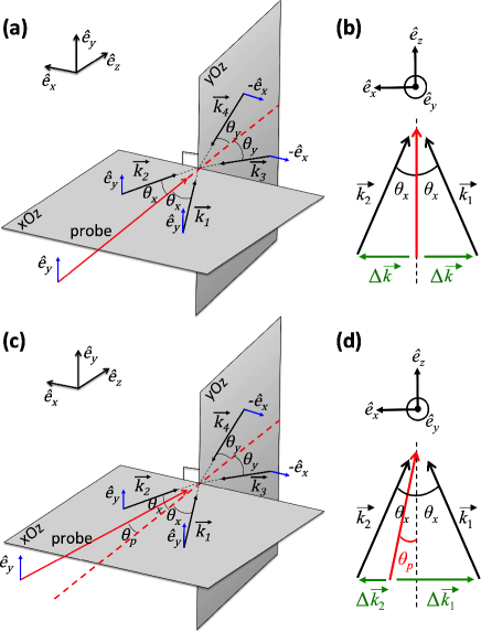
Figure 1: 3D-lin$\perp$lin tetrahedral lattice illuminated by a weak probe. (a) and (b) depict the case of space periodic driving: The probe propagates along the $z$-axis, which is the lattice symmetry axis. (c) and (d) show the case where the space period of the driving is not a multiple of the period of the underlying optical lattice: The probe propagates along a direction forming an angle $\theta_{p}$ with the $z$-axis. Here, $|\Delta{\vec{k}_{1}}|=k_{0}+k_{l}\sin\theta_{p}$ and $|\Delta{\vec{k}_{2}}|=k_{0}-k_{l}\sin\theta_{p}$, where $k_{l}$ is the laser wave number, and $k_{0}=k_{l}\sin\theta_{x}$.

Following previous studies, [8, 37, 14, 13, 15, 28, 31], we focus on movement along one of the directions, taken as the $x$-axis. The optical potential associated with the above setup is then given by (after taking $y=z=0$)

$$U_{\pm}(x,t)=\frac{U_{0}}{2}\Big{[}-\frac{3}{2}-\frac{1}{2}\cos(2k_{0}x)\pm\cos(k_{0}x)$$

$$+\varepsilon_{p}\cos(-k_{0}x+k_{l}\sin\theta_{p}x-\delta_{p}t)$$

$$+\varepsilon_{p}\cos(k_{0}x+k_{l}\sin\theta_{p}x-\delta_{p}t)$$

$$\pm\varepsilon_{p}\cos(k_{l}\sin\theta_{p}x-\delta_{p}t)\Big{]},$$ (1)

where $k_{0}=k_{l}\sin\theta_{x}$, $k_{l}=\omega_{l}/c$ is the laser beam wave number, $\delta_{p}=\omega_{p}-\omega_{l}$ is a small probe detuning relative to the lattice ($\delta_{p}/\omega_{l}\ll 1$) , $U_{0}=-16\hbar\Delta^{\prime}_{0}/3$, with $\Delta^{\prime}_{0}$ ($<0$) being the light-shift per lattice field, and $\varepsilon_{p}=E_{p}/(2E_{0})$.

The optical well-depth $U_{0}$ defines a vibrational frequency associated with an atom of mass $m_{a}$ oscillating at the bottom of a well,

$$\Omega_{x}=k_{x}\sqrt{3U_{0}/2m_{a}}=4\sin\theta_{x}\sqrt{|\Delta_{0}^{\prime}|\omega_{r}},$$ (2)

where $\omega_{r}=\hbar k_{l}^{2}/(2m_{a})$ is the recoil frequency.

The probe perturbation in (1) appears in three terms: A modulation propagating to the right with phase velocity $v_{1}=\delta_{p}/(k_{0}+k_{l}\sin\theta_{p})$, another to the left with velocity $v_{2}=-\delta_{p}/(k_{0}-k_{l}\sin\theta_{p})$, and a third moving with velocity $v_{3}=\delta_{p}/(k_{l}\sin\theta_{p})$. Each of these terms will produce an excitation of atomic density waves on their own. Thus, for the sake of simplicity, we consider them separately in the theoretical considerations that follow.

The first system model to consider, denoted as case (a), is the following optical potential, which accounts for the third probe term in (1), and is given by

$$U_{\pm}^{(a)}(x,t)=\frac{U_{0}}{2}\Big{[}-\frac{3}{2}-\frac{1}{2}\cos(2k_{0}x)\pm\cos(k_{0}x)$$

$$\pm\varepsilon_{p}\cos(k_{p}x-\delta_{p}t+\phi_{p}),\Big{]},$$ (3)

where $k_{p}=k_{l}\sin\theta_{p}$, and $\phi_{p}$ is a probe phase which has been introduced for convenience in the analytical calculations to be presented below. Here the potential perturbation changes sign with the specific atomic state. Terms of this kind are also generated with a $x$-polarized probe.

In addition, we consider the case of the following optical potential, denoted as case (b), which accounts for the first two probe terms in (1), and is given by:

$$U_{\pm}^{(b)}(x,t)=\frac{U_{0}}{2}\Big{[}-\frac{3}{2}-\frac{1}{2}(2k_{0}x)\pm\cos(k_{0}x)$$

$$+\varepsilon_{p}\cos(k_{p}x-\delta_{p}t+\phi_{p}),\Big{]},$$ (4)

By setting $k_{p}=|\Delta{\vec{k}_{1}}|=k_{0}+k_{l}\sin\theta_{p}$, or $k_{p}=|\Delta{\vec{k}_{2}}|=-(k_{0}-k_{l}\sin\theta_{p})$, we can study the effects introduced by the first and second probe terms, respectively. If $\theta_{p}=0$, $|\Delta{\vec{k}_{1,2}}|=|\Delta{\vec{k}}|=k_{0}$. See Figs. 1 (b) and (d) for an illustration of $\Delta{\vec{k}_{1}}$ and $\Delta{\vec{k}_{2}}$.

Note the on-axis case $\theta_{p}=0$, recently investigated in Refs. [28, 31], produces a space periodic perturbation, because the wave number of the driving field $k_{p}$ is the same as that of the underlying lattice, $k_{0}$. On the other hand, a probe angle $0<\theta_{p}<\pi/2$ such that $k_{p}/k_{0}$ is an irrational ratio produces a space quasiperiodic drive.

In the semi-classical approximation [36], the atoms in the ground state $|\pm\rangle$ are described by the phase space density $P_{\pm}(x,p,t)$ at the position $x$ with momentum $p$, which satisfies the following coupled Fokker-Planck equations

$$\left[\frac{\partial}{\partial t}+\frac{p}{m_{a}}\frac{\partial}{\partial x}-U_{\pm}^{\prime}(x)\frac{\partial}{\partial p}\right]P_{\pm}=$$

$$-\gamma_{\pm}(x)P_{\pm}+\gamma_{\mp}(x)P_{\mp}+\frac{\partial^{2}}{\partial p^{2}}\left[D_{0}P_{\pm}\right],$$ (5)

where $U_{\pm}^{\prime}=\partial U_{\pm}/\partial x$, and

$$\gamma_{\pm}(x)=g_{0}\pm g_{1}\cos(k_{0}x)+g_{2}\cos(2k_{0}x)$$ (6)

are the transition rates between the ground state sublevels, defined in terms of $\Gamma^{\prime}$, the photon scattering rate per lattice beam, as $g_{0}=2\Gamma^{\prime}/3$, $g_{1}=8\Gamma^{\prime}/9$, $g_{2}=2\Gamma^{\prime}/9$, and $D_{0}=5\hbar^{2}k_{0}^{2}\Gamma^{\prime}/18$ is a noise strength describing the random momentum jumps that result from the interaction with the photons. As in [31], we are neglecting the probe contribution to the transition rates, the radiation forces, and noise terms, since their effect is observed to be small in the simulations.

Directed motion is characterized by the current, defined as the average atomic velocity

$$\langle v\rangle=\lim_{t\rightarrow\infty}\frac{\langle[x(t)-x(0)]\rangle}{t}=$$

$$\lim_{t\rightarrow\infty}\frac{1}{t}\int_{0}^{t}\!\!dt^{\prime}\int\!\!dx\int\!\!dp\,\frac{p}{m_{a}}[P_{+}(x,p,t^{\prime})+P_{-}(x,p,t^{\prime})].$$ (7)

II Analytical results

Following the method presented in Ref. [31], we Fourier-decompose the current in (7) into contributions arising from atomic density modes excited by the probe. Using $l$, $n$, $m$ to denote the mode numbers, so that the mode has a frequency $\omega=l\delta_{p}$ and wave number $k=nk_{0}+mk_{p}$, we obtain, in terms of the amplitudes of the excited atomic density waves,

$$P^{\pm}[l,n,m]=\frac{\delta_{p}}{2\pi}\int_{0}^{2\pi/\delta_{p}}\!\!\!dt\,e^{-il\delta_{p}t}\int\!dx\,e^{i(nk_{0}+mk_{p})x}$$

$$\int\!dp\,P_{\pm}(x,p,t),$$ (8)

the following expansion for the current for case (b), i.e., the setup defined by (4) for the $U^{(b)}$ system,

$$\langle v\rangle_{\mathrm{(b)}}=\frac{m_{a}}{m_{a}F_{0}g_{1}-2D_{0}k_{0}}\Bigg{[}$$

$$-\frac{\text{Im}\left[P_{+}[0,1,0]\right]F_{0}\left(8g_{0}^{2}-4g_{2}^{2}/3+F_{0}k_{0}/(2m_{a})\right)}{k_{0}}$$

$$+\frac{\text{Im}\left[P_{+}[0,2,0]\right]F_{0}\left(-4g_{0}g_{1}{-8g_{1}g_{2}/3}+F_{0}k_{0}/m_{a}\right)}{k_{0}}$$

$$+\frac{\text{Im}\left[P_{+}[0,3,0]\right]F_{0}\left(-16g_{0}g_{1}/3-2g_{2}^{2}-3F_{0}k_{0}/(2m_{a})\right)}{k_{0}}$$

$$+\frac{\text{Im}\left[P_{+}[0,4,0]\right]F_{0}\left(-2g_{1}g_{2}/3+F_{0}k_{0}/(2m_{a})\right)}{k_{0}}$$

$$-\frac{\text{Im}\left[P_{+}[0,5,0]\right]F_{0}2g_{2}^{2}}{3k_{0}}+\frac{\text{Im}\left[e^{i\phi_{p}}P_{+}[1,-2,1]\right]F_{0}F_{p}(2k_{0}-k_{p})}{2m_{a}k_{p}}$$

$$+\frac{\text{Im}\left[e^{i\phi_{p}}P_{+}[1,-1,1]\right]F_{0}F_{p}(-k_{0}+k_{p})}{m_{a}k_{p}}$$

$$+\frac{\text{Im}\left[e^{i\phi_{p}}P_{+}[1,0,1]\right]2F_{p}k_{0}\delta_{p}^{2}}{k_{p}^{2}}$$

$$+\frac{\text{Im}\left[e^{i\phi_{p}}P_{+}[1,1,1]\right]F_{0}F_{p}(k_{0}+k_{p})}{m_{a}k_{p}}$$

$$-\frac{\text{Im}\left[e^{i\phi_{p}}P_{+}[1,2,1]\right]F_{0}F_{p}(2k_{0}+k_{p})}{2m_{a}k_{p}}$$

$$+\frac{\text{Im}\left[e^{i2\phi_{p}}P_{+}[2,0,2]\right]F_{p}^{2}k_{0}}{m_{a}k_{p}},\Bigg{]}.$$

where the force amplitudes $F_{0}=k_{0}U_{0}/2$ and $F_{p}=U_{0}\varepsilon_{p}k_{p}/2$. Equation (II) is valid for an arbitrary $k_{p}$, including the periodic case $k_{p}=k_{0}$, which was validated numerically in Ref. [31].

Similar expressions are found for case (a), defined by Eq. (3), which are reported in the appendix. The main difference between the cases (a) and (b), defined by (3) and (4), respectively, is that case (a) provides different expressions for the generic case $k_{p}\neq k_{0}$ and the special case $k_{p}=k_{0}$. In the expansion for the periodic case $k_{p}=k_{0}$, reported in (A), there are more terms —thus more atomic wave modes activated— than in the quasiperiodic case where $k_{p}/k_{0}$ is an irrational ratio, reported in (A). These extra terms cannot be obtained from (A) after taking the limit $k_{p}\rightarrow k_{0}$.

Furthermore, (A) shows some apparent singularities in the form of coefficients with denominators proportional to $k_{0}-k_{p}$ or $k_{0}-2k_{p}$, and thus apparently problematic in the periodic limits $k_{p}\rightarrow k_{0}$ and $k_{p}\rightarrow 2k_{0}$. This could suggest a special sensitivity to the periodic/quasiperiodic transition, similar to that observed in the case of time quasiperiodicity [6, 7, 39, 33, 34, 35], where the large sensitivity in the system response to time quasiperiodic forces is known to yield sub-Fourier resonances.

However, our numerical results, reported in the following section, shows that this is not the case, and the transition is smooth. This is possible because the amplitudes of the modes involved decay to zero as (or stronger than) $k_{0}-k_{p}$ or $k_{0}-2k_{p}$, thus removing any possible singularity in the periodic cases $k_{0}=k_{p}$ or $k_{0}=2k_{p}$.

The analytical expansions, though, still provide a useful decomposition into atomic waves of directed transport, and are used in the following sections to interpret the atomic transport provoked by the probe.

III Numerical results

Numerical solutions of the equation (5) are obtained by generating a large number of individual atomic trajectories $x_{j}(\sigma_{j}(t),t)$, where $\sigma_{j}(t)=+1$ or $-1$ is the occupied state at time $t$ in that trajectory, using a stochastic algorithm [40]. Averages are computed using over $1.5\times 10^{6}$ trajectories. Following Ref. [31], the atomic mode amplitudes (8) are calculated via the formula,

$$P_{\pm}[l,n,m]=\lim_{l^{\prime}\rightarrow\infty}\frac{\delta_{p}}{2\pi l^{\prime}N}\times$$

$$\sum_{j=1}^{N}\int_{0}^{2\pi l^{\prime}/\delta_{p}}\!\!\!dt\,e^{i[(nk_{0}+mk_{p})x_{j}(\sigma_{j}(t),t)-l\delta_{p}t]}\delta_{\sigma_{j}(t),\pm 1}.$$ (10)

In all simulations, units are defined such that $m_{a}=\hbar=k_{l}=1$. In these units, the optical lattice parameters were fixed to $U_{0}=200$, $\Gamma^{\prime}=2.85$.

We start by first studying the system sensitivity to the transition between space periodic and quasiperiodic driving. We chose the $U^{(a)}$ system in (3) (i.e., case (a)), because it gives different expansions in the periodic $k_{p}=k_{0}$ and quasiperiodic ($k_{p}$ and $k_{0}$ incommensurate) cases. Specifically, Eq. (A) indicates a potential singularity when $k_{p}\rightarrow k_{0}$ in the mode $\mathrm{Re}[P_{+}[1,-1,1]]$ due to the presence of $(k_{p}-k_{0})$ in the denominator of the coefficient.

Figure 2 shows the current and the mode contributions to the current, given by (A), as a function of $k_{p}$ around the periodic case $k_{p}=k_{0}$. No mode or contribution is observed to act abruptly, on the contrary, they all are seen to behave smoothly. The potential singularity in the mode $\mathrm{Re}[P_{+}[1,-1,1]]$ does not actually occur, because the mode amplitude itself tends to zero in the limit $k_{p}\rightarrow k_{0}$ as $(k_{p}-k_{0})$, such that its current contribution is finite, as seen in Fig. 2.

Similar features are observed near $k_{p}=2k_{0}$, demonstrating that the transition from space quasiperiodicity to periodicity is smooth.

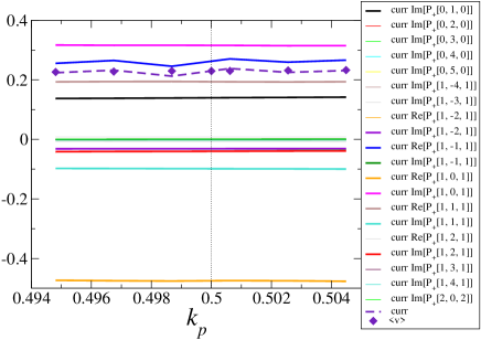
Figure 2: Smooth space quasiperiodicity. Current and mode contributions to the current as a function of the driving wave number $k_{p}$ for the $U^{(a)}$ system in (3) (i.e., case (a)), with $\delta_{p}=7.5$, $\epsilon_{p}=0.8$, $\theta_{x}=30^{0}$ (thus $k_{0}=0.5$), and $\phi_{p}=0$. Each mode $(l,n,m)$ has a frequency $\omega=l\delta_{p}$ and wave number $k=nk_{0}+mk_{p}$. Mode amplitudes are measured in the simulation via (10), and their precise contribution to the current determined using (A). The dashed line is the sum of all current contributions, and the diamonds are the current calculated from its definition (7). Units are defined such that $m_{a}=\hbar=k_{l}=1$.

Next, in order to understand how Brillouin modes are generated, we study the atomic waves when varying the driving frequency $\delta_{p}$. A series of resonances, that is, local maxima at certain values of the driving frequencies is observed, allowing for a proper rationalization of the transport mechanisms and the experimental results.

Figure 3 shows the current as a function of $\delta_{p}$ for several values of the driving amplitude $\varepsilon_{p}$ in the $U^{(b)}$ system defined by (4) (i.e., case (b)), with space periodic driving $k_{p}=k_{0}$, for several values of the driving amplitude $\varepsilon_{p}$.

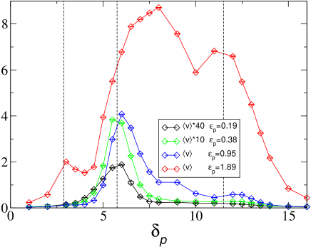
Figure 3: The atomic current is plotted for the case of space periodic driving as a function of the driving frequency $\delta_{p}$ in the $U^{(b)}$ system defined by (4) (i.e., case (b)), with $\theta_{x}=25^{0}$, $\phi_{p}=\pi$, for several values of the driving amplitude $\varepsilon_{p}$. The driving wave number is fixed to $k_{p}=k_{0}$. Dotted vertical lines are placed at $\omega_{0}=5.75$, $\omega_{0}/2$, and $2\omega_{0}$. Resonances at multiples and sub-multiples of the intrinsic frequency $\omega_{0}$ are observed.

A peak at $\delta_{p}=\omega_{0}=5.75$ is observed, common to all curves, except the one corresponding to the largest value of $\varepsilon_{p}$, which is shifted to higher frequency values, about $\delta_{p}\sim 7.5$. This peak is not far from the vibrational frequency (2) associated with linear oscillations in the optical wells, $\Omega_{x}=7.3$ with the parameter values mentioned above for the simulations. In Fig. 3 the presence of additional peaks at about $\omega_{0}/2$ and $2\omega_{0}$ can be seen. This behavior is not uncommon, in rocked ratchets the current is also observed [33] to peak at multiples and sub-multiples, in general a fractional number, of an intrinsic frequency.

As the driving wave number $k_{p}$ is varied, so does the phase velocity of the propagating perturbation $v_{p}=\delta_{p}/k_{p}$. It is expected [8] that a peak is produced when this phase velocity matches the velocity

$$v_{0}=\omega_{0}/k_{0}.$$ (11)

The intrinsic velocity $v_{0}$ is associated with an average drift in one direction due to half oscillations in a well, followed by transitions between the atomic states [8]. This velocity matching ($vm$) mechanism thus yields a peak at

$$(\delta_{p})_{vm}=\omega_{0}k_{p}/k_{0}.$$ (12)

The numerical results, presented in Fig. 4 do not contradict this picture.

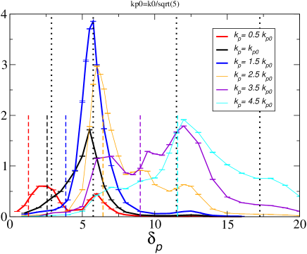
Figure 4: Same as in Fig. 3 (i.e., for the $U^{(b)}$ system in (4), case (b)), but this time for space quasiperiodic driving with $k_{p0}=k_{0}/\sqrt{5}$. The current is plotted for several values of the driving wave number, $k_{p}=0.5k_{p0},k_{p0},1.5k_{p0},2.5k_{p0},3.5k_{p0}$, and $4.5k_{p0}$. In all cases the driving amplitude $\epsilon_{p}$ was varied so that $\epsilon_{p}k_{p}=0.8$, thus keeping the force amplitude $F_{p}$ fixed. As in Fig. 3, dotted vertical lines are placed at $\omega_{0}=5.75$, $\omega_{0}/2$, and $2\omega_{0}$, plus an additional one at $3\omega_{0}$. The truncated vertical dashed lines correspond to the shifted values $(\delta_{p})_{vm}=\omega_{0}k_{p}/k_{0}$.

However, it is somehow obscured by the above mentioned frequency peaking at a fractional ratio of the intrinsic frequency. For example, let’s consider the case of space-quasiperiodic driving with $k_{p}=0.5k_{p0}$, where $k_{p0}\equiv k_{0}/\sqrt{5}$. In this case, the current-vs-$\delta_{p}$ curve displays a peak near ($\delta_{p})_{vm}$, but it is also leaning towards $\omega_{0}/2$. The curves for $k_{p}=k_{p0}$ and $k_{p}=1.5k_{p0}$ show no velocity matching shift, just peaking at the value $\omega_{0}$. The curve $k_{p}=2.5k_{p0}$ does peak at ($\delta_{p})_{vm}$, but this value is very near $\omega_{0}$ in this case. It also shows a small peak at about $1.5\omega_{0}$. In the case $k_{p}=3.5k_{p0}$, the frequency ($\delta_{p})_{vm}$ lies between the peaks at $\omega_{0}$ and $2\omega_{0}$. The corresponding curve peaks at $\omega_{0}$, ($\delta_{p})_{vm}$ (or $1.5\omega_{0}$, since they are very near here), and $2\omega_{0}$. The curve $k_{p}=4.5k_{p0}$ offers a clear confirmation of the velocity matching mechanism, because it shows no clear peak at $\omega_{0}$, and a distinct one at ($\delta_{p})_{vm}$, which is also close to $2\omega_{0}$.

Overall, the discussed shift due to velocity matching is clearly at play in the system, but the shift takes place through local maxima at a fractional ratio of the intrinsic frequency $\omega_{0}$.

We may then wonder how a particular atomic mode is affected by the above discussed resonances. Figure 5 shows the results for the case $k_{p}=3.5k_{p0}$, which was chosen because the current shows three peaks in Figure 4, at $\omega_{0}$, $1.5\omega_{0}\approx$ ($\delta_{p})_{vm}$, and $2\omega_{0}$. The plot shows peaks at these frequency values at most of the atomic modes, behaving very similarly all of them. Moreover, an extra peak in most of them is also visible at $\delta_{p}=3\omega_{0}$, a peak which is difficult to appreciate in the current plot, Fig. 4.

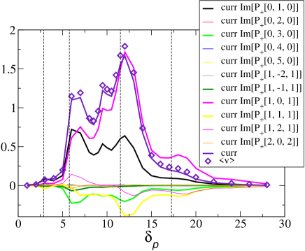
Figure 5: Current and mode contributions to the current as a function of the driving frequency $\delta_{p}$ for the quasiperiodic case $k_{p}=3.5k_{p0}$ shown in Fig. 4 (for the $U^{(b)}$ system in (4), case (b)). As in Fig. 4, dotted vertical lines are placed at $\omega_{0}=5.75$, $\omega_{0}/2$, $2\omega_{0}$, and $3\omega_{0}$.

IV Experiment

Our experiments are performed on ⁸⁵Rb atoms in a dilutely occupied dissipative 3D lattice in a tetrahedral lin$\perp$lin configuration, as in Fig. 1. Directed motion is produced by the weak $\hat{y}$-polarized probe which makes an angle $\theta_{p}$ with the $z$-axis. The probe frequency $\omega_{p}$ is scanned around the (fixed) frequency $\omega_{l}$ of the lattice beams, and probe transmission is measured as a function of probe detuning $\delta=\omega_{p}-\omega_{l}$. As in Ref. [28], $\delta/\omega_{L}<10^{-9}$. Here, the intensity ratio of probe to lattice (sum of all four beams) is less than $3\%$,

In accordance with the notation used in Ref. [11, 28], $\Delta_{0}^{\prime}\equiv\Delta{s_{0}}/2$, and $\Gamma^{\prime}\equiv\Gamma{s_{0}/2}$ where $s_{0}\equiv(I/I_{sat})/(1+4\Delta^{2}/\Gamma^{2})$ is just the saturation parameter. For the $F_{g}=3\rightarrow F_{e}=4$ transition in ⁸⁵Rb, $I_{sat}=1.67$ mW/cm² for $\sigma$-light, $\Gamma/2\pi$ is the natural linewidth for ⁸⁵Rb (6.07 MHz), and $\omega_{r}/2\pi$ is the recoil frequency (3.86 kHz). In our experiment, $\theta_{x}=\theta_{y}=25^{0}$, and each lattice beam has intensity $I=6.22$ mW/cm², a $1/e^{2}$-diameter 5.4 mm (the probe diameter is 1.4 mm), and red-detuning $\Delta=8.75\Gamma$. In order to determine the intensity $I$ that actually illuminates the atoms, care is taken to account for the intensity loss through the windows of the vacuum cell that houses the lattice, and the background Rb vapor. These values yield $s_{0}=0.012$, $\Gamma^{\prime}/2\pi=36.4$ kHz, and a well-depth $U_{0}=445\,\hbar\omega_{r}$. Using the definition of the recoil frequency just after (2), and setting $\hbar=m_{a}=k_{l}=1$ as in the simulations, we find this $U_{0}$-value corresponds to 223, and $\Gamma^{\prime}$, in units of the recoil frequency, corresponds to 4.72 - these values are comparable to those assumed in the simulations in Sec. III.

Figs. 6(a) and (b) show distinctly different probe transmission spectra for $\theta_{p}=0$ and $17.5^{0}$, respectively. The peaks in the spectra correspond to photons absorbed from a lattice beam and emitted via stimulated emission into the probe, while dips correspond to photons absorbed from the probe and emitted into a lattice beam.

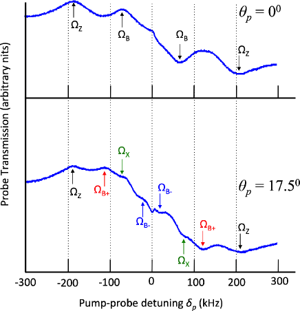
Figure 6: Probe transmission spectra measured for (a) $\theta_{p}=0$ (space periodic case $k_{p}=k_{0}$) and (b) $17.5^{0}$ ($k_{p}$ not a multiple of $k_{0}$). The resonance peaks have been identifed as $\Omega_{Z}$, $\Omega_{B}$, $\Omega_{X}$, and $\Omega_{B\pm}$.

We discuss first the periodic case shown in Fig. 6 (a), in which the probe is aligned with the $z$-axis ($\theta_{p}=0$). This system was analyzed in detail in Ref. [28], where it was confirmed that the spectral features denoted as $\Omega_{Z}$ arise from probe-induced Raman transitions between adjacent vibrational levels corresponding to oscillations along the $z$-axis in each well, and the $\Omega_{B}$ features arise from Brillouin-like directed transport along the $\pm x$-directions.

Indeed, the vibrational frequency in the $z$-direction is determined in the system model by [28]

$$\Omega_{z}=2(\mbox{cos}\,{\theta_{x}}+\mbox{cos}\,{\theta_{y}})\sqrt{2|\Delta_{0}^{\prime}|\,\omega_{r}},$$ (13)

thus yielding $\Omega_{z}=2\pi(180$ kHz), which is in reasonable agreement with the observed value of about 200 kHz. Moreover, Eq. (2) yields a vibrational frequency $\Omega_{x}/2\pi=60$ kHz, which is very close to the observed value for $\Omega_{B}/2\pi$. This $\Omega_{x}$-value equals 15.5 $\omega_{r}$, which in simulation units corresponds to 7.8, not far from the 7.3 value mentioned in Sec. III. The agreement between the predicted and observed values for $\Omega_{x}$ and $\Omega_{B}$ is remarkable considering that the theory assumed a $F_{g}=1/2\rightarrow F_{e}=3/2$ atom.

It is important to note that even though $\Omega_{B}$ coincides with $\Omega_{x}$, the spectral features at $\Omega_{B}$ in Fig. 6(a) could not arise from intrawell oscillatory motion in the $x$-direction, owing to the fact that adjacent vibrational levels are of opposite parity, and hence the overlap integral of the probe operator (i.e., the lattice-probe interference term) between these two levels is zero (because the interference term goes as $\vec{E}_{0}\cdot{\vec{E}^{*}}_{p}$ and is quadratic in $x$ for a probe that propagates purely along $\hat{z}$; here $\vec{E}_{0}$ and $\vec{E}_{p}$ are the lattice and probe electric field amplitudes, respectively, [28]).

In this space periodic case $\theta_{p}=0$, the three probe terms of (1) reduces to a single perturbation propagating with phase velocity $v_{0}=\delta_{p}/k_{0}$, like in the 1D model (4) with $k_{p}=k_{0}$, whose numerical results are shown in Fig. 3. In agreement with the experimental results of Fig. 6 (a), the theoretical model predicts a dominant peak at about $\omega_{0}$, which is identified with $\Omega_{x}$. The secondary peaks observed at other multiples of $\omega_{0}$ in Fig. 3 for certain values of the driving amplitudes are absent in Fig. 6 (a), though.

Let us turn, then, our attention to the case where $k_{p}\neq k_{0}$, shown in Fig. 6 (b). Equation (1) indicates that the probe driving produces three perturbations propagating with phase velocities $v_{1}=\delta_{p}/(k_{0}+k_{l}\sin\theta_{p})$, $v_{2}=-\delta_{p}/(k_{0}-k_{l}\sin\theta_{p})$, and $v_{3}=\delta_{p}/(k_{l}\sin\theta_{p})$. The first two perturbations are the result of the interference between the $\hat{y}$-polarized probe and the $\hat{y}$-polarized lattice beams $\vec{k}_{1}$, $\vec{k}_{2}$, as depicted in Fig. 1. However, the third perturbation, being produced by the interference of the probe with the $\hat{x}$-polarized lattice beams $\vec{k}_{3}$ and $\vec{k}_{4}$, is not expected to show up in the transmission spectrum depicted in Fig. 6 (b) because of Doppler broadening [9, 28]. Specifically, the $z$-component of the motion makes the scattered field vary randomly, being responsible for a wash-out of the spectral features related to the $x$-motion [9] due to the perturbation propagating with velocity $v_{3}$. In other words, the pump-probe measurements shown here are sensitive only to the $U^{(b)}$-perturbation defined by (4) (i.e., case (b)), and are not sensitive to the $U^{(a)}$-perturbation defined by (3) under case (a). As indicated in Sec. III, the simulations in Figs. 3 - 5 all pertain to case (b).

Case (b) refers to the first two perturbations in (1). Following the velocity matching argument discussed in Sec. III, we expect a peak for the driving frequency values where the intrinsic velocity $\pm v_{0}$ (11) matches the velocity of the propagating perturbation, thus leading to two possible values for the probe detuning $\delta_{p}$, located on either side of $\Omega_{x}$:

$$\delta_{1}=\Omega_{x}\frac{\sin\theta_{x}+\sin\theta_{p}}{\sin\theta_{x}},$$ (14)

$$\delta_{2}=\Omega_{x}\frac{\sin\theta_{x}-\sin\theta_{p}}{\sin\theta_{x}},$$ (15)

where we have identified the vibrational frequency $\omega_{0}=\Omega_{x}$. The theoretical analysis of Sec. III also predicts a peak at a multiple of the vibrational frequency, specially around the central value at $\Omega_{x}$, as seen in Fig. 4.

In order to confirm the angle-dependencies in (14) and (15), we have carried out several measurements with varying values of the probe angle $\theta_{p}$. The results are plotted in Fig. 7.

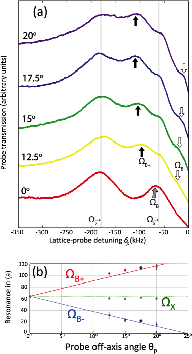
Figure 7: (a) Pump-probe spectra taken at different probe angles $\theta_{p}$ for the lattice in Fig. 1(a). The vertical lines demarcate the fixed vibrational frequencies $\Omega_{z}$ and $\Omega_{x}$. At $\theta_{p}=0$, the gray arrow denotes the Brillouin resonance $\Omega_{B}$ that coincides with $\Omega_{x}$. At $\theta_{p}\neq 0$, the black and white arrows denote Brillouin resonances $\Omega_{B+}$ and $\Omega_{B-}$, respectively. (b) $\Omega_{B+}$ and $\Omega_{B-}$ depart from $\Omega_{x}$ in accordance with Eqs. (14) and (15), respectively: The solid lines are the theoretical predictions from the equations. The two black-circled datapoints in (b) correspond to the spectrum in Fig. 6(b). It takes 10 ms to generate those spectra, and each datapoint here is an average of at least five scans.

The solid lines in Fig. 7 (b) confirm the analytical predictions of Eqs. (14) and (15), with $\delta_{1}$ and $\delta_{2}$ explaining the observed peaks $\Omega_{B+}$ and $\Omega_{B-}$, respectively, that are seen in Fig. 7 (a) and Fig. 6 (b). The quantitative agreement is remarkable, specially taking into account that the theory is based on a 1D model with a simplified atomic transition.

The theory also offers an explanation [9] for the fact that the amplitudes of the $\Omega_{B-}$ resonance are seen to be smaller than the $\Omega_{B+}$ ones. Since the spatial period $2\pi/(k_{0}-k_{l}\sin\theta_{p})$ associated for the $\Omega_{B-}$ motion is larger than that of $\Omega_{B+}$, $2\pi/(k_{0}+k_{l}\sin\theta_{p})$, the sequence of half oscillations and well-transfers for $\Omega_{B-}$ is more likely to be interrupted by random photon recoils associated with the Sisyphus process, causing a larger damping of the directed propagation. For the $\Omega_{B+}$ resonance, $k_{p}=k_{0}+k_{l}\sin\theta_{p}$, yielding $k_{p}/k_{p0}$-values corresponding to the four angles from $12.5^{0}$ to $20^{0}$ as 3.4, 3.6, 3.8, and 4.1, respectively. Note that the first two values are close to the $k_{p}/k_{p0}$-value of 3.5 in Fig. 5, which predicts peaks in the directed propagation at $\omega_{0}$, $(\delta_{p})_{vm}\approx 1.5\omega_{0}$, and $2\omega_{0}$. The peak at $\omega_{0}=\Omega_{x}\approx 2\pi\,(60\mbox{kHz})$ is certainly observed in Fig. 7 (a) and (b), as are single peaks at approximately 105 kHz and 110 kHz for $\theta_{p}=12.5^{0}$ and $15^{0}$, respectively. The experiment does not resolve each of these single peaks into possible components at the numerical peaks, but the observed single-peak values lie in between these, not too far from them. Thus the experimental findings in Fig. 7 (a-b) and the numerical simulations in Fig. 5 do not contradict each other.

Finally, figs. 7(a) and (b) show consistently a peak at $\delta_{p}=\Omega_{x}$, regardless of the specific value of $\theta_{p}$. While symmetry consideration for $\theta_{p}=0$ forbids the appearance of a resonance in the spectrum due to localized vibrations about the well bottoms, that is not the case for $\theta_{p}\neq 0$. However, as shown in Sec. III for the 1D theoretical model, the observed peak may well also be due to directed motion.

V Conclusions

We have studied the atomic waves generated in a dissipative optical lattice under a weak beam that produces a directed current which travels perpendicular to the direction of travel of the probe.

On the theoretical side, a minimal 1D model of the experimental setup is studied in detail to elucidate the mechanisms of transport. An analytical method based on a Fourier decomposition of the current is applied to study the case when the driving potential perturbation has a spatial period which is the same as that of the underlying lattice, a case of space periodic driving, and when both periods are incommensurate, the regime of space quasiperiodic driving.

It is numerically demonstrated that the transition between both regimes is smooth, despite the fact that the expansion for one of the probe perturbations is different in each regime. When the frequency of the probe is varied, the current, and more specifically the mode amplitudes that contribute to the current, show several peaks. One set is identified with a multiple of the intrinsic frequency $\omega_{0}$, and another is associated with a velocity matching mechanism, in which the velocity of the propagating modulation matches up with the average velocity of the atom in its intrawell oscillation. Both mechanisms are seen at play in both the space periodic and space quasiperiodic regime, and even at play at the same time, since the shift due to velocity matching is observed to take place through local maxima at a fractional ratio of the intrinsic frequency $\omega_{0}$.

The pump-probe experiments confirm many of the above predictions. In the case of space-periodic driving $k_{p}=k_{0}$, with a weak beam that is aligned with the lattice symmetry axis, the probe transmission spectrum indeed reveals a dominant peak at $\omega_{0}$, shown in Fig. 6(a), that corresponds to a propagating Brillouin-like mode in a direction perpendicular to probe propagation. These observations are borne out by the numerical predictions in Fig. 3, although secondary peaks predicted at multiples and sub-multiples of $\omega_{0}$ were not observed in this work. In the case of driving with the weak beam incident at angle $\theta_{p}$ with the lattice symmetry axis, the spectrum reveals a peak at $\omega_{0}$, and also additional peaks where the velocity matching mechanism above is satisfied, as shown in Fig. 6(b). The angle-dependence of these additional spectral features, which correspond to two distinct propagating modulations with different spatial periods, is shown in Fig. 7 to be in accordance with the analytical predictions. These findings are not contradicted by the numerical predictions in Figs. 4 and 5, although it was not experimentally possible to tease apart the contributions to the observed resonances made by $(\delta_{p})_{vm}$ versus those made by multiples and sub-multiples of $\omega_{0}$. We hope that the new understanding of Brillouin transport modes gained here would pave the road toward ratcheting of cold atoms confined in a weakly modulated optical lattice, along a precisely predictable, arbitrary direction [7].

VI Acknowledgments

This work is supported by the Army Research Office under award/contract number W911NF2110120 and the Ministerio de Ciencia e Innovación of Spain of Spain, Grant No. PID2019-105316GB-I00 (DC). We thank the Instrumentation Laboratory at Miami University for electronics and LabView support. We gratefully acknowledge invaluable assistance in the lab from Ian Dilyard and Jordan Churi.

Appendix A Further analytical results

The setup defined by case (a) in (3) requires different expressions for the quasiperiodic ($k_{p}/k_{0}$ irrational) and periodic $k_{p}=k_{0}$ cases. The calculation proceeds along the same lines sketched in [31]. The atomic state symmetry produced by the probe for setup (3) is given by

$$P_{-}[l,n,m]=(-1)^{n+l}P_{+}[l,n,m],$$ (16)

which can be also written as

$$P_{-}[l,n,m]=(-1)^{n+m}P_{+}[l,n,m],$$ (17)

the latter being a useful expression in the special (periodic) case $k_{p}=k_{0}$.

In the quasiperiodic case we find

$$\langle v\rangle_{\mathrm{(a)}}=\frac{m_{a}}{m_{a}F_{0}g_{1}-2D_{0}k_{0}}\Bigg{[}$$

$$-\frac{\text{Im}\left[P_{+}[0,1,0]\right]F_{0}\left(8g_{0}^{2}-4g_{2}^{2}/3+F_{0}k_{0}/(2m_{a})\right)}{k_{0}}$$

$$+\frac{\text{Im}\left[P_{+}[0,2,0]\right]F_{0}\left(-4g_{0}g_{1}{-8g_{1}g_{2}/3}+F_{0}k_{0}/m_{a}\right)}{k_{0}}$$

$$+\frac{\text{Im}\left[P_{+}[0,3,0]\right]F_{0}\left(-16g_{0}g_{1}/3-2g_{2}^{2}-3F_{0}k_{0}/(2m_{a})\right)}{k_{0}}$$

$$+\frac{\text{Im}\left[P_{+}[0,4,0]\right]F_{0}\left(-2g_{1}g_{2}/3+F_{0}k_{0}/(2m_{a})\right)}{k_{0}}$$

$$-\frac{\text{Im}\left[P_{+}[0,5,0]\right]F_{0}2g_{2}^{2}}{3k_{0}}+\frac{\text{Im}\left[e^{i\phi_{p}}P_{+}[1,-4,1]\right](2F_{p}g_{2}^{2}k_{0})}{(2k_{0}-k_{p})k_{p}}$$

$$+\frac{\text{Im}\left[e^{i\phi_{p}}P_{+}[1,-3,1]\right]2F_{p}g_{1}g_{2}k_{0}}{(2k_{0}-k_{p})k_{p}}$$

$$+\frac{\text{Im}\left[e^{i\phi_{p}}P_{+}[1,-2,1]\right]}{(2k_{0}-k_{p})k_{p}^{2}}[8F_{p}g_{0}g_{2}(-k_{0}^{2}+k_{0}k_{p})$$

$$+F_{0}F_{p}(2k_{0}^{2}k_{p}-2k_{0}k_{p}^{2}+k_{p}^{3}/2)/m_{a}]$$

$$-\frac{\text{Re}\left[e^{i\phi_{p}}P_{+}[1,-2,1]\right]4F_{p}g_{2}k_{0}(k_{0}-k_{p})\delta_{p}}{(2k_{0}-k_{p})k_{p}^{2}}$$

$$+\frac{\text{Im}\left[e^{i\phi_{p}}P_{+}[1,-1,1]\right]}{(2k_{0}-k_{p})k_{p}^{2}}F_{p}\Bigg{[}4g_{0}g_{1}k_{0}(-2k_{0}+k_{p})$$

$$+2g_{1}g_{2}k_{0}k_{p}+\frac{F_{0}}{m_{a}}(-2k_{0}^{2}k_{p}+3k_{0}k_{p}^{2}-k_{p}^{3})\Bigg{]}$$

$${\color[rgb]{0,0,1}-\frac{\text{Re}\left[e^{i\phi_{p}}P_{+}[1,-1,1]\right]2F_{p}g_{1}k_{0}(k_{0}-2k_{p})\delta_{p}}{(k_{0}-k_{p})k_{p}^{2}}}$$

$$-\frac{\text{Im}\left[e^{i\phi_{p}}P_{+}[1,0,1]\right]}{(2k_{0}-k_{p})k_{p}^{2}(2k_{0}+k_{p})}F_{p}[g_{0}^{2}(32k_{0}^{3}-8k_{0}k_{p}^{2})$$

$$-4g_{2}^{2}k_{0}k_{p}^{2}+\delta_{p}^{2}(-8k_{0}^{3}+2k_{0}k_{p}^{2})]$$

$$-\frac{\text{Re}\left[e^{i\phi_{p}}P_{+}[1,0,1]\right]8F_{p}g_{0}k_{0}\delta_{p}}{k_{p}^{2}}$$

$$+\frac{\text{Im}\left[e^{i\phi_{p}}P_{+}[1,1,1]\right]}{(2k_{0}+k_{p})k_{p}^{2}}F_{p}[-4g_{0}g_{1}k_{0}(2k_{0}+k_{p})$$

$$-2g_{1}g_{2}k_{0}k_{p}+F_{0}(2k_{0}^{2}k_{p}+3k_{0}k_{p}^{2}+k_{p}^{3})/m_{a}]$$

$$-\frac{\text{Re}\left[e^{i\phi_{p}}P_{+}[1,1,1]\right]2F_{p}g_{1}k_{0}(k_{0}+k_{p})\delta_{p}}{(k_{0}+k_{p})k_{p}^{2}}$$

$$+\frac{\text{Im}\left[e^{i\phi_{p}}P_{+}[1,2,1]\right]}{(2k_{0}+k_{p})k_{p}^{2}}[8F_{p}g_{0}g_{2}(-k_{0}^{2}-k_{0}k_{p})$$

$$+F_{0}F_{p}(-2k_{0}^{2}k_{p}-2k_{0}k_{p}^{2}-k_{p}^{3}/2)/m_{a}]$$

$$-\frac{\text{Re}\left[e^{i\phi_{p}}P_{+}[1,2,1]\right]4F_{p}g_{2}k_{0}(k_{0}+k_{p})\delta_{p}}{(2k_{0}+k_{p})k_{p}^{2}}$$

$$-\frac{\text{Im}\left[e^{i\phi_{p}}P_{+}[1,3,1]\right]2F_{p}g_{1}g_{2}k_{0}}{(2k_{0}+k_{p})k_{p}}$$

$$-\frac{\text{Im}\left[e^{i\phi_{p}}P_{+}[1,4,1]\right](2F_{p}g_{2}^{2}k_{0})}{(2k_{0}+k_{p})k_{p}}$$

$$+\frac{\text{Im}\left[e^{i2\phi_{p}}P_{+}[2,0,2]\right]F_{p}^{2}k_{0}}{m_{a}k_{p}}\Bigg{]}.$$

Equation (A) is not valid when the ratio $k_{p}/k_{0}$ is a rational number. In this case there are resonances which require a special derivation [31]. An indication of this fact is that the coefficient associated with the mode amplitude $\mathrm{Re}[P_{+}[1,-1,1]]$ goes to infinity in the limit $k_{p}\rightarrow k_{0}$, whereas the actual coefficient when computed directly in the case $k_{p}=k_{0}$ remains finite, as shown in Eq. (A).

The full expansion in the periodic case $k_{p}=k_{0}$ is given by

$$\langle v\rangle_{\mathrm{(a)}}=\frac{m_{a}}{m_{a}F_{0}g_{1}-2D_{0}k_{0}}\Bigg{[}$$

$${\color[rgb]{0,0,1}-\frac{\text{Re}\left[P_{+}[0,1,0]\right]F_{0}\left(F_{p}^{2}g_{1}\right)}{m_{a}\delta_{p}}}$$

$$-\frac{\text{Im}\left[P_{+}[0,1,0]\right]F_{0}\left(8g_{0}^{2}-4g_{2}^{2}/3+F_{0}k_{0}/(2m_{a})\right)}{k_{0}}$$

$$+\frac{\text{Im}\left[P_{+}[0,2,0]\right]F_{0}\left(-4g_{0}g_{1}{-8g_{1}g_{2}/3}+F_{0}k_{0}/m_{a}\right)}{k_{0}}$$

$$+\frac{\text{Im}\left[P_{+}[0,3,0]\right]F_{0}\left(-16g_{0}g_{1}/3-2g_{2}^{2}-3F_{0}k_{0}/(2m_{a})\right)}{k_{0}}$$

$$+\frac{\text{Im}\left[P_{+}[0,4,0]\right]F_{0}\left(-2g_{1}g_{2}/3+F_{0}k_{0}/(2m_{a})\right)}{k_{0}}$$

$$-\frac{\text{Im}\left[P_{+}[0,5,0]\right]F_{0}2g_{2}^{2}}{3k_{0}}+\frac{\text{Im}\left[e^{i\phi_{p}}P_{+}[1,-4,1]\right](2F_{p}g_{2}^{2})}{k_{0}}$$

$${\color[rgb]{0,0,1}+\frac{\text{Re}\left[e^{i\phi_{p}}P_{+}[1,-3,1]\right](F_{0}F_{p}g_{1})}{m_{a}\delta_{p}}}$$

$$+\frac{\text{Im}\left[e^{i\phi_{p}}P_{+}[1,-3,1]\right]2F_{p}g_{1}g_{2}}{k_{0}}$$

$$+\frac{\text{Im}\left[e^{i\phi_{p}}P_{+}[1,-2,1]\right]F_{0}F_{p}}{2m_{a}}$$

$${\color[rgb]{0,0,1}-\frac{\text{Re}\left[e^{i\phi_{p}}P_{+}[1,-2,1]\right]F_{0}F_{p}g_{1}}{m_{a}\delta_{p}}}$$

$$+\frac{\text{Im}\left[e^{i\phi_{p}}P_{+}[1,-1,1]\right]}{k_{0}}F_{p}(-4g_{0}g_{1}+2g_{1}g_{2})$$

$${\color[rgb]{0,0,1}-\frac{\text{Re}\left[e^{i\phi_{p}}P_{+}[1,-1,1]\right]2F_{p}g_{1}\delta_{p}}{k_{0}}}$$

$$-\frac{\text{Im}\left[e^{i\phi_{p}}P_{+}[1,0,1]\right]}{3k_{0}}2F_{p}(12g_{0}^{2}-2g_{2}^{2}-3\delta_{p}^{2})$$

$$-\frac{\text{Re}\left[e^{i\phi_{p}}P_{+}[1,0,1]\right]({\color[rgb]{0,0,1}-F_{0}F_{p}g_{1}k_{0}/\delta_{p}}+8F_{p}g_{0}\delta_{p})}{k_{0}}$$

$$+\frac{\text{Im}\left[e^{i\phi_{p}}P_{+}[1,1,1]\right]}{(3k_{0}}F_{p}[-12g_{0}g_{1}-2g_{1}g_{2}+6F_{0}k_{0}/m_{a}]$$

$$-\frac{\text{Re}\left[e^{i\phi_{p}}P_{+}[1,1,1]\right]{\color[rgb]{0,0,1}(F_{p}F_{0}g_{1}k_{0}/\delta_{p}}+3F_{p}g_{1}\delta_{p})}{k_{0}}$$

$$+\frac{\text{Im}\left[e^{i\phi_{p}}P_{+}[1,2,1]\right]}{(6k_{0}}F_{p}(-32g_{0}g_{2}-9F_{0}k_{0}/m_{a})$$

$$-\frac{\text{Re}\left[e^{i\phi_{p}}P_{+}[1,2,1]\right]8F_{p}g_{2}\delta_{p}}{3k_{0}}$$

$$-\frac{\text{Im}\left[e^{i\phi_{p}}P_{+}[1,3,1]\right]2F_{p}g_{1}g_{2}}{3k_{0}}$$

$$-\frac{\text{Im}\left[e^{i\phi_{p}}P_{+}[1,4,1]\right](2F_{p}g_{2}^{2})}{3k_{0}}$$

$${\color[rgb]{0,0,1}+\frac{\text{Im}\left[e^{i2\phi_{p}}P_{+}[2,-1,2]\right]F_{p}^{2}g_{1}}{\delta_{p}}}$$

$$+\frac{\text{Im}\left[e^{i2\phi_{p}}P_{+}[2,0,2]\right]F_{p}^{2}}{m_{a}}\Bigg{]}\quad(k_{p}=k_{0}).$$

Terms in (A), which are not directly obtained from (A) after taking the limit $k_{p}\rightarrow k_{0}$, have been highlighted in blue. Note there are also terms in the quasiperiodic case (A) which are singular when $k_{p}\rightarrow 2k_{0}$. But again, this singularity is removed in the exact limit $k_{p}=2k_{0}$.

References

- Heinrich et al. [2021] A. Heinrich, W. D. Oliver, L. M. K. Vandersypen, A. Ardavan, R. Sessoli, D. Loss, A. B. Jayich, J. Fernandez-Rossier, A. Laucht, and A. Morello, Quantum-coherent nanoscience, Nat. Nanotechnol. 16, 1318 (2021).
- Wang et al. [2018] Y. Wang, S. Subhankar, P. Bienias, M. Łącki, T.-C. Tsui, M. A. Baranov, A. V. Gorshkova, P. Zoller, J. V. Porto, and S. Rolston, Dark state optical lattice with sub-wavelength spatial structure, Phys. Rev. Lett. 120, 083601 (2018).
- Łącki et al. [2016] M. Łącki, M. A. Baranov, H. Pichler, , and P. Zoller, Nanoscale dark state optical potentials for cold atoms, Phys. Rev. Lett. 117, 233001 (2016).
- Miles et al. [2013] J. A. Miles, Z. J. Simmons, and D. D. Yavuz, Subwavelength localization of atomic excitation using electromagnetically induced transparency, Phys. Rev. X 3, 031014 (2013).
- Zemanek et al. [2020] P. Zemanek, G. Volpe, A. Jonas, and O. Brzobohaty, Perspective on light-induced transport of particles: from optical forces to phoretic motion, Adv. Opt. Photonics 11, 577 (2020).
- Cubero and Renzoni [2016] D. Cubero and F. Renzoni, Brownian Ratchets: From Statistical Physics to Bio and Nano-motors (Cambridge University Press, Cambridge, 2016).
- Cubero and Renzoni [2012] D. Cubero and F. Renzoni, Control of transport in two-dimensional systems via dynamical decoupling of degrees of freedom with quasiperiodic driving fields, Phys. Rev. E 86, 056201 (2012).
- Courtois et al. [1996] J. Y. Courtois, S. Guibal, D. R. Meacher, P. Verkerk, and G. Grynberg, Propagating elementary excitation in a dilute optical lattice, Phys. Rev. Lett. 77, 40 (1996).
- Jurczak et al. [1998] C. Jurczak, J.-Y. Courtois, B. Desruelle, C. Westbrook, , and A. Aspect, Spontaneous light scattering from propagating density fluctuations in an optical lattice, Eur. Phys. J. D 1, 53 (1998).
- Mennerat-Robilliard et al. [1999] C. Mennerat-Robilliard, D. Lucas, S. Guibal, J. Tabosa, C. Jurczak, J.-Y. Courtois, and G. Grynberg, Ratchet for cold rubidium atoms: The asymmetric optical lattice, Phys. Rev. Lett. 82, 851 (1999).
- Grynberg and Robilliard [2001] G. Grynberg and C. Robilliard, Cold atoms in dissipative optical lattices, Phys. Rep. 355, 335 (2001).
- Schiavoni et al. [2002a] M. Schiavoni, L. Sanchez-Palencia, F. Carminati, F. Renzoni, and G. Grynberg, Dark propagation modes in optical lattices, Phys. Rev. A 66, 053821 (2002a).
- Sanchez-Palencia et al. [2002] L. Sanchez-Palencia, F.-R. Carminati, M. Schiavoni, F. Renzoni, and G. Grynberg, Brillouin propagation modes in optical lattices: Interpretation in terms of nonconventional stochastic resonance, Phys. Rev. Lett. 88, 133903 (2002).
- Carminati et al. [2003] F.-R. Carminati, M. Schiavoni, Y. Todorov, F. Renzoni, and G. Grynberg, Pump-probe spectroscopy of atoms cooled in a 3d lin-perp-lin optical lattice, Eur. Phys. J. D 22, 311 (2003).
- Sanchez-Palencia and Grynberg [2003] L. Sanchez-Palencia and G. Grynberg, Synchronization of hamiltonian motion and dissipative effects in optical lattices: Evidence for a stochastic resonance, Phys. Rev. A 68, 023404 (2003).
- Schiavoni et al. [2003] M. Schiavoni, L. Sanchez-Palencia, F. Renzoni, and G. Grynberg, Phase control of directed diffusion in a symmetric optical lattice, Phys. Rev. Lett. 90, 094101 (2003).
- Jones et al. [2004] P. H. Jones, M. Goonasekara, and F. Renzoni, Rectifying fluctuations in an optical lattice, Phys. Rev. Lett. 93, 073904 (2004).
- Gommers et al. [2005] R. Gommers, S. Bergamini, and F. Renzoni, Dissipation-induced symmetry breaking in a driven optical lattice, Phys. Rev. Lett. 95, 073003 (2005).
- Gommers et al. [2006] R. Gommers, S. Denisov, and F. Renzoni, Quasiperiodically driven ratchets for cold atoms, Phys. Rev. Lett. 96, 240604 (2006).
- Gommers et al. [2007] R. Gommers, M. Brown, and F. Renzoni, Symmetry and transport in a cold atom ratchet with multifrequency driving,, Phys. Rev. A 75, 053406 (2007).
- Gommers et al. [2008] R. Gommers, V. L. andM. Brown, and F. Renzoni, Gating ratchet for cold atoms, Phys. Rev. Lett. 100, 040603 (2008).
- Lebedev and Renzoni [2009] V. Lebedev and F. Renzoni, Two-dimensional rocking ratchet for cold atoms, Phys. Rev. A 80, 023422 (2009).
- Cubero et al. [2010] D. Cubero, V. Lebedev, and F. Renzoni, Current reversals in a rocking ratchet: dynamical vs symmetry-breaking mechanisms, Phys. Rev. E 82, 041116 (2010).
- Wickenbrock et al. [2011] A. Wickenbrock, D. Cubero, N. A. A. Wahab, P. Phoonthong, and F. Renzoni, Current reversals in a rocking ratchet: The frequency domain, Phys. Rev. E 84, 021127 (2011).
- Hagman et al. [2011] H. Hagman, M. Zelan, C. M. Dion, and A. Kastberg, Directed transport with real-time steering and drifts along predesigned paths using a brownian motor,, Phys. Rev. A 83, 020101(R) (2011).
- Zelan et al. [2011] M. Zelan, H. Hagman, G. Labaigt, S. Jonsell, , and C. M. Dion, Experimental measurement of efficiency and transport coherence of a cold-atom brownian motor in optical lattices, Phys. Rev. A 83, 020102(R) (2011).
- Wickenbrock et al. [2012] A. Wickenbrock, P. C. Holz, N. A. A. Wahab, P. Phoonthong, D. Cubero, and F. Renzoni, Vibrational mechanics in an optical lattice: Controlling transport via potential renormalization, Phys. Rev. Lett. 108, 020603 (2012).
- Staron et al. [2022] A. Staron, K. Jiang, C. Scoggins, D. Wingert, D. Cubero, and S. Bali, Observation of stochastic resonance in directed propagation of cold atoms, Phys. Rev. Research 4, 043211 (2022).
- [29] H. J. Metcalf and P. van der Straten, Cooling and Trapping.
- Hodapp et al. [1995] T. W. Hodapp, C. Gerz, C. Furtlehner, C. I. Westbrook, W. D. Phillips, and J. Dalibard, Three-dimensional spatial diffusion in optical molasses, Appl. Phys. B 60, 135 (1995).
- Cubero [2023] D. Cubero, Brillouin propagation modes of cold atoms undergoing sisyphus cooling, Phys. Rev. E 107, 034102 (2023).
- Lutz and Renzoni [2013] E. Lutz and F. Renzoni, Beyond boltzmann–gibbs statistical mechanics in optical lattices, Nature Physics 9, 615 (2013).
- Cubero et al. [2014] D. Cubero, J. Casado-Pascual, and F. Renzoni, Irrationality and quasiperiodicity in driven nonlinear systems, Phys. Rev. Lett. 112, 174102 (2014).
- Cubero and Renzoni [2018] D. Cubero and F. Renzoni, Asymptotic theory of quasiperiodically driven quantum systems, Phys. Rev. E 97, 062139 (2018).
- Cubero et al. [2018] D. Cubero, G. Robb, and F. Renzoni, Avoided crossing and sub-fourier-sensitivity in driven quantum systems, Phys. Rev. Lett. 121, 213904 (2018).
- Petsas et al. [1999] K. Petsas, G. Grynberg, and J.-Y. Courtois, Semiclassical monte carlo approaches for realistic atoms in optical lattices, Eur. Phys. J. D 6, 29 (1999).
- Schiavoni et al. [2002b] M. Schiavoni, F.-R. Carminati, L. Sanchez-Palencia, F. Renzoni, and G. Grynberg, Stochastic resonance in periodic potentials: Realization in a dissipative optical lattice, Europhys. Lett. 59, 493 (2002b).
- Note [1] This definition of the probe detuning corrects a sign error in Ref. [28].
- Casado-Pascual et al. [2013] J. Casado-Pascual, D. Cubero, and F. Renzoni, Universal asymptotic behavior in nonlinear systems driven by a two-frequency forcing, Phys. Rev. E 88, 062919 (2013).
- Kloeden and Platen [1992] P. Kloeden and E. Platen, Numerical Solution of Stochastic Differential Equations (Springer, New York, 1992).