Top tree amplitudes for higher order calculations

Abstract

We present compact analytic results for tree-level amplitudes containing a $t\bar{t}$ pair accompanied by up to four massless partons, $t\bar{t}gg$, $t\bar{t}ggg$, $t\bar{t}gggg$, $t\bar{t}q\bar{q}$, $t\bar{t}q\bar{q}g$, $t\bar{t}q\bar{q}gg$ and $t\bar{t}q\bar{q}q^{\prime}\bar{q}^{\prime}$. The results, obtained using BCFW on-shell recursion, are based both on previous published results and on the new calculations performed in this paper. These amplitudes are sufficient to calculate the production of a $t\bar{t}$ pair and zero, one, or two light parton jets, with the option to include the tree-level decays $t\to b\nu e^{+}$ and $\bar{t}\to\bar{b}e^{-}\bar{\nu}$ efficiently. Our results are part of the NNLO corrections to $t\bar{t}$ production including the decay correlations for on-shell top quarks.

1 Introduction

The calculation of tree-graph amplitudes for massless particles is radically simplified by the exploitation of spinor methods DeCausmaecker:1981jtq ; Berends:1981uq ; Kleiss:1985yh ; Xu:1986xb ; Mangano:1990by ; Dixon:1996wi . However it is less widely appreciated that even in the presence of masses, spinor techniques can lead to compact expressions for tree-graph amplitudes.

This has recently been demonstrated for amplitudes containing a $t\bar{t}$-pair and $(n-2)$ gluons Ochirov:2018uyq where beautiful results have been obtained for all $n\geq 4$ for two particular helicity combinations. The two cases comprise the amplitude with all gluons with identical helicity, and the amplitude with one opposite-helicity gluon color-adjacent to one of the quarks. In a second paper results have been provided for amplitudes involving two massive quark-antiquark pairs and an arbitrary number of identical helicity gluons Lazopoulos:2021mna . These relations are proved using Britto-Cachazo-Feng-Witten (BCFW) recursion Britto:2004ap ; Britto:2005fq . The other required amplitudes for $t\bar{t}ggg$ and some additional amplitudes for $t\bar{t}gggg$ can be obtained using Bern-Carrasco-Johansson (BCJ) relations Bern:2008qj ; Bern:2019prr .

Automatic procedures to calculate tree (and one-loop) graphs are available Maltoni:2002qb ; Gleisberg:2008fv ; Actis:2016mpe ; Buccioni:2019sur . Nevertheless it seemed opportune to apply the theoretical results described above for the concrete case of $t\bar{t}$+jets, supplementing the results given in ref. Ochirov:2018uyq with explicit expressions for $t\bar{t}q\bar{q}$ and the five- and six-parton amplitudes, $t\bar{t}q\bar{q}g$, $t\bar{t}q\bar{q}gg$ and $t\bar{t}q\bar{q}q^{\prime}\bar{q}^{\prime}$. This is particularly useful because amplitude expressions allow the inclusion of the tree-level decay of the top quark Kleiss:1988xr .

The BCFW technique allows the iterative construction of higher point amplitudes starting from three-point amplitudes evaluated at complex momenta for both massless and massive Badger:2005jv ; Badger:2005zh ; Ozeren:2006ft ; Huang:2012gs ; Ochirov:2018uyq ; Lazopoulos:2021mna amplitudes. Since the amplitudes are constructed using on-shell results, they are free of the redundant gauge degrees of freedom which are present in a normal quantum field theory calculation. Our results are presented using the formalism of Arkani-Hamed, Huang and Huang (AHH) Arkani-Hamed:2017jhn , who have extended the spinor-helicity formalism for massless particles. In their formalism the covariance properties of the amplitudes under little group rotations are made manifest by the addition of a $SU(2)$ little group index. The resulting Spin-spinors carry an $SU(2)$ index ($I$) in addition to the Lorentz group SL$(2,\mathbb{C})$ indices, $(\alpha,{\dot{\alpha}})$. From the point of view of the amplitude program, which asserts that amplitudes calculated recursively using on-shell ingredients are more fundamental than their quantum field theory analogues, the extension to massive particles is an important and necessary step.

Our aim in this paper is more prosaic; we want to investigate the benefits for top quark physics of analytic tree-level amplitudes calculated using BCFW techniques. The work of BCFW and BCJ has shown that full amplitudes can be calculated from a limited number of ingredients. At low perturbative order analytic results can be computationally more efficient (see for example ref. Lazopoulos:2021mna ) than results based on off-shell Berends-Giele recursion Berends:1987me , which is often the automatic procedure of choice for the calculation of tree graphs. These amplitudes will be incorporated in MCFM MCFM , exploiting the possibility of including the tree-level decay of the top quark with decay correlations at essentially zero cost Kleiss:1988xr . Finally, we note that compact low order tree-graph results can be useful ingredients for loop calculations via unitarity, see for example refs. Bern:1995db ; Budge:2020oyl .

1.1 Plan of the paper

Section 2 gives an introduction to the massless and massive spinor formalism, following the method of AHH for the massive case. Section 3 addresses the definition of color-ordered primitives and the BCJ relations between them. The basic 3-parton building blocks for the BCFW recursion are also presented here. Section 4 illustrates the use of BCFW recursion for the calculation of $A_{4}(\bm{1},3_{g}^{+},4_{g}^{+},\bm{2}_{{\bar{Q}}})$ and $A_{4}(\bm{1},3_{g}^{+},4_{g}^{-},\bm{2}_{{\bar{Q}}})$, and presents a full set of results for the 4-parton amplitudes. Section 5 uses the results of the previous two sections to calculate the 5-parton amplitude $A_{5}(\bm{1},\bm{2}_{{\bar{Q}}},3_{q}^{-},4_{\bar{q}}^{+},5_{g}^{+})$ to further illustrate the application of BCFW techniques. Sections 6 and 7 present the results for all the 5-parton and 6-parton amplitudes. Both sections contain a description of the color decomposition of the amplitude, the form of the squared amplitude after summing over colors, a complete set of results for the subamplitudes in terms of massless and massive spinors for all helicity combinations of the massless particles and a description of the BCJ relations between the sub-amplitudes, if applicable. In section 8 we give an explicit representation of the Spin-spinors that is closely connected to the Kleiss-Stirling method Kleiss:1986qc and review the implementation of tree-level top-quark decay. In section 9 we draw some conclusions. Appendix A derives the results needed for the calculation in the Spin-spinor formalism and appendix B gives an alternative color decomposition for $Q\bar{Q}q\bar{q}gg$ amplitudes.

2 Spin-spinor formalism

In this section we will introduce the essence of the Spin-spinor formalism of Arkani-Hamed, Huang and Huang (AHH) Arkani-Hamed:2017jhn . A more detailed exposition of this formalism is given in refs. Ochirov:2018uyq ; Christensen:2018zcq ; Christensen:2019mch ; Lazopoulos:2021mna . Appendix A gives a detailed derivation of the results that we will need for our calculation.

2.1 Massless partons

We consider a spinor state $|p\rangle_{\beta}$ which is a solution to the massless Weyl equation $p^{{\dot{\alpha}}\beta}\,|p\rangle_{\beta}=0$ where $p^{{\dot{\alpha}}\beta}=p^{\mu}\sigma_{\mu}^{{\dot{\alpha}}\beta}$ is derived from the four-momentum $p^{\mu}$ of the particle. The indices ${\dot{\alpha}}$ and $\beta$ are the SL$(2,\mathbb{C})$ Lorentz group indices that are normally superfluous in the angle and square bracket formalism, but we sometimes find it convenient to retain them here. Since the particle is massless, $p^{{\dot{\alpha}}\beta}$ is a rank one matrix and is expressible as

$$p^{{\dot{\alpha}}\beta}=|p]^{\dot{\alpha}}\langle p|^{\beta},\;\;$$ (1)

which is clearly invariant under the little group rescaling

$$\langle p|^{\beta}\to t\,\langle p|^{\beta}\,,\quad\quad|p]^{\dot{\alpha}}\to\frac{1}{t}|p]^{\dot{\alpha}}\,.$$ (2)

The spinors are in the fundamental representation of the group SL$(2,\mathbb{C})$ and the particular components are indicated by indices ${\dot{\alpha}},\beta$. For a massless particle we can go to a frame in which the momentum is directed along the $z$ direction $p=(E,0,0,E)$. The little group is thus the group of rotations in the $x,y$ plane, namely $SO(2)\equiv U(1)$.The great utility of the spinor formalism derives from the fact that amplitudes are directly functions of spinor helicity variables.

2.2 Massive partons

The extension of this formalism to massive particles notes that the little group in this case can be deduced in the rest frame of the particle. In the rest frame the little group is the set of rotations in $3$ dimensions, namely $SO(3)\equiv SU(2)$. Amplitudes can now be expressed in terms of Spin-spinors which transform as a direct product of the $SU(2)$ spin group tensor and the SL$(2,\mathbb{C})$ Lorentz group. These Spin-spinors are denoted by $|\bm{p}^{I}\rangle^{\beta}$ and $|\bm{p}^{I}]^{\dot{\alpha}}$. In the angle and square bracket notation combination rules for the dotted and undotted SL$(2,\mathbb{C})$ indices are mandated by the angle and square brackets, so they can be dropped in spinor products. Amplitudes involving massive particles, with momenta $p_{1}$ and $p_{2}$ are naturally expressed in terms of spinor products such as $\langle\bm{1}^{I}\bm{2}_{J}\rangle$, $\left[\bm{1}^{I}\bm{2}_{J}\right]$ since these spinor products reflect the little group transformation properties of the amplitudes themselves.

The Spin-spinors so defined satisfy a number of relations that are necessary to perform the BCFW recursion. These identities are,

$$\begin{aligned} |\bm{p}^{I}\rangle_{\;\!\!\alpha}\;\![\bm{p}_{I}|_{{\dot{\beta}}}&=+p_{\alpha{\dot{\beta}}}\\ |\bm{p}^{I}]^{{\dot{\alpha}}}\>\!\langle\bm{p}_{I}|^{\beta}&=-p^{{\dot{\alpha}}\beta}\\ |\bm{p}^{I}\rangle_{\;\!\!\alpha}\langle\bm{p}_{I}|^{\beta}&=+m\>\!\delta_{\alpha}^{\beta}\\ |\bm{p}^{I}]^{{\dot{\alpha}}}\;\>\!\![\bm{p}_{I}|_{{\dot{\beta}}}&=-m\>\!\delta^{{\dot{\alpha}}}_{{\dot{\beta}}}\end{aligned}\qquad\quad\begin{aligned} |\bm{p}_{I}\rangle_{\;\!\!\alpha}\;\![\bm{p}^{I}|_{{\dot{\beta}}}&=-p_{\alpha{\dot{\beta}}}\\ |\bm{p}_{I}]^{{\dot{\alpha}}}\>\!\langle\bm{p}^{I}|^{\beta}&=+p^{{\dot{\alpha}}\beta}\\ |\bm{p}_{I}\rangle_{\;\!\!\alpha}\langle\bm{p}^{I}|^{\beta}&=-m\>\!\delta_{\alpha}^{\beta}\\ |\bm{p}_{I}]^{{\dot{\alpha}}}\;\>\!\![\bm{p}^{I}|_{{\dot{\beta}}}&=+m\>\!\delta^{{\dot{\alpha}}}_{{\dot{\beta}}}\end{aligned}\qquad\quad\begin{aligned} p^{{\dot{\alpha}}\beta}|\bm{p}^{I}\rangle_{\;\!\!\beta}&=-m|\bm{p}^{I}]^{{\dot{\alpha}}}\\ p_{\alpha{\dot{\beta}}}|\bm{p}^{I}]^{{\dot{\beta}}}&=-m|\bm{p}^{I}\rangle_{\;\!\!\alpha}\\ \langle\bm{p}^{I}|^{\alpha}p_{\alpha{\dot{\beta}}}&=+m[\bm{p}^{I}|_{{\dot{\beta}}}\\ [\bm{p}^{I}|_{{\dot{\alpha}}}p^{{\dot{\alpha}}\beta}&=+m\langle\bm{p}^{I}|^{\beta}\end{aligned}\qquad\quad$$ (3)

The derivation of these relations is presented in Appendix A. The SU(2) indices are raised and lowered using the two-dimensional totally antisymmetric tensor $\epsilon^{IJ}$.

We adopt the convention that,

$$|-p\rangle=-|p\rangle\,,\quad\quad|-p]=|p]\,.$$ (4)

In this paper we calculate amplitudes will all momenta outgoing. With this convention we have that

$$\gamma_{\mu}p^{\mu}+m=\left(\begin{matrix}|-p_{I}]^{\dot{\alpha}}[p^{I}|_{\dot{\beta}}&\;|-p_{I}]^{\dot{\alpha}}\langle p^{I}|^{\beta}\\ |-p_{I}\rangle_{\alpha}[p^{I}|_{\dot{\beta}}&\;|-p_{I}\rangle_{\alpha}\langle p^{I}|^{\beta}\end{matrix}\right)\,,$$ (5)

which shows that sewing together amplitudes in the BCFW method, where one line must perforce have a negative momentum, reproduces the numerator of the massive fermion propagator.

Armed with the basic results for the 3-point vertices involving massive and massless particles we can construct higher point tree-level amplitudes using BCFW recursion. In addition we can illustrate the BCJ relations between the analytical results that we calculate.

3 Color and counting of primitives

It is well known that for the case of pure gluon scattering, the color-trace decomposition into color-ordered primitives is Mangano:1990by ,

$${\cal A}_{n}(1_{g},2_{g},\ldots n_{g})=\!\!\sum_{\sigma\in S_{n-1}(\{2,\dots,n\})}\!\!\!\operatorname*{Tr}\!\big{(}t^{C_{1}}t^{C_{\sigma(2)}}\dots t^{C_{\sigma(n)}}\big{)}\bar{A}_{n}(1,\sigma(2),\dots,\sigma(n))\,,$$ (6)

where the sum is over $(n-1)!$ primitives, since the cyclicity of the trace allows one to fix the first argument. This decomposition has the disadvantage that the color coefficients are not all linearly independent. Consequently the color-ordered sub-amplitudes are not the minimal set. Indeed for the pure gluon case, the color sub-amplitudes defined in Eq. (6) are related by the Kleiss-Kuijf (KK) relations Kleiss:1988ne , which reduce the number of independent primitives to $(n-2)!$. It was subsequently observed by Del Duca, Dixon and Maltoni DelDuca:1999rs that the color decomposition

$${{\cal A}}_{n}(1_{g},2_{g},\ldots n_{g})=\!\!\sum_{\sigma\in S_{n-2}(\{3,\dots,n\})}\!\!\!\big{(}T^{C_{\sigma(3)}}\dots T^{C_{\sigma(n)}}\big{)}_{C_{1}C_{2}}A_{n}(1,2,\sigma(3),\dots,\sigma(n))\,,$$ (7)

where $T$ are $SU(3)$ matrices in the adjoint representation, contains only linearly independent color structures and automatically reduces the number of independent color-subamplitudes to $(n-2)!$.

In this paper we will be dealing with amplitudes with one or more quark lines. For the case of one quark line, the trace representation

$${{\cal A}}_{n}(\bm{1}_{Q},\bm{2}_{{\bar{Q}}},3_{g}\ldots n_{g})=\!\!=\!\!\sum_{\sigma\in S_{n-2}(\{3,\dots,n\})}\!\!\!\big{(}T^{C_{\sigma(3)}}\dots T^{C_{\sigma(n)}}\big{)}_{x_{1}x_{2}}A_{n}(\bm{1}_{Q},\bm{2}_{{\bar{Q}}},\sigma(3),\dots,\sigma(n))\,,$$ (8)

is free of further relations of the KK type. In addition to pure gluon processes, color decompositions for processes involving one quark line have been considered in ref. DelDuca:1999rs . In the case where we consider more than one quark line the equivalent color decompositions have been given in refs. Ellis:2011cr ; Johansson:2015oia ; Melia:2013bta ; Melia:2013epa ; Melia:2015ika . Table 1 presents the number of primitive color sub-amplitudes after application of all KK-type relations, for the top pair production amplitudes that we consider in this paper.

$n$	$k$	$n_{g}$	$n_{P}$
$\#$ of partons	$\#$ of quark pairs	$\#$ of gluons	$\#$ of primitives
4	1	2	2
5	1	3	6
6	1	4	24
4	2	0	1
5	2	1	3
6	2	2	12
6	3	0	4

Table 1: Number of independent primitive amplitudes $n_{P}=(n-2)!/k!$, after imposition of KK-type constraints. $n$ is the total number of partons, and $k$ is the number of distinguishable quark pairs.

3.1 Relations between the kinematic part of tree amplitudes

Bern, Carrasco and Johansson (BCJ) have discovered additional relations obeyed by amplitudes involving external gluons. The quark-gluon BCJ relations, for one or more massive quark lines, are given by the general formula Bern:2008qj ; Johansson:2015oia ; Bern:2019prr ,

$$\sum_{i=2}^{n-1}\Big{(}\sum_{j=2}^{i}s_{jn}-m_{j}^{2}\Big{)}A_{n}(\bm{1}_{Q},\bm{2}_{{\bar{Q}}},\dots i,n_{g},i+1,\dots,n-1)=0\,.$$ (9)

where particle $n$ is strictly a gluon, while the remaining $(n-1)$ particles can be of any type: quark/antiquark/gluon. Table 2 gives results for the number of primitives after imposition of BCJ relations.

$n$	$k$	$n_{g}$	$n_{P}$
$\#$ of partons	$\#$ of quark pairs	$\#$ of gluons	$\#$ of primitives
4	1	2	1
5	1	3	2
6	1	4	6
4	2	0	1
5	2	1	2
6	2	2	6
6	3	0	4

Table 2: Number of independent primitive amplitudes $n_{P}$ after imposition of KK and BCJ constraints. $n$ is the total number of partons, and $k$ is the number of distinguishable quark pairs. For $k=1$ this is $n_{P}=(n-3)!$, while for $k\geq 2$ $n_{P}=(n-3)!\,(2k-2)/k!$. Adapted from ref. Johansson:2015oia .

3.2 Three parton amplitudes

In this section we provide the basic building blocks for 3-point amplitudes. These are necessary in order to start the BCFW recursion. For the $ggg$ process we have,

$${\cal A}_{3}(1_{g}^{-},2_{g}^{-},3_{g}^{+})=g\tilde{f}^{{C_{1}}{C_{2}}{C_{3}}}\;\frac{\langle 12\rangle^{3}}{\langle 23\rangle\,\langle 31\rangle}=-ig\big{(}\operatorname*{Tr}\{t^{C_{1}}t^{C_{2}}t^{C_{3}}\}-\operatorname*{Tr}\{t^{C_{1}}t^{C_{3}}t^{C_{2}}\})\;\frac{\langle 12\rangle^{3}}{\langle 23\rangle\,\langle 31\rangle}\,.$$ (10)

For the $Qg{\bar{Q}}$ process we have,

$${\cal A}_{3}(\bm{1}_{x_{1}},3_{C},\bm{2}_{x_{2}})=g\,(t^{C})_{x_{1}x_{2}}\,A_{3}(\bm{1}_{Q},3,\bm{2}_{{\bar{Q}}})$$ (11)

where,

$$-iA_{3}(\bm{1}_{Q},3^{+},\bm{2}_{{\bar{Q}}}) = -\frac{\big{(}[\bm{1}3]\langle q\bm{2}\rangle+\langle\bm{1}q\rangle[3\bm{2}]\big{)}}{\langle q3\rangle}$$ (12)

$$= -\frac{\big{(}\left\langle\bm{1}|\bm{1}|3\right]\langle q\bm{2}\rangle-\langle\bm{1}q\rangle\left[3|\bm{2}|\bm{2}\right\rangle\big{)}}{m\langle q3\rangle}=-\frac{\langle\bm{1}\bm{2}\rangle\langle q|\bm{1}|3]}{m\langle q3\rangle}\,,$$

$$-iA_{3}(\bm{1}_{Q},3^{-},\bm{2}_{{\bar{Q}}}) = -\frac{\big{(}\langle\bm{1}3\rangle[q\bm{2}]+[\bm{1}q]\langle 3\bm{2}\rangle\big{)}}{[3\;\!q]}$$ (13)

$$= -\frac{\big{(}[\bm{1}|\bm{1}|3\rangle[q\bm{2}]-[\bm{1}q]\left\langle 3|\bm{2}|\bm{2}\right]\big{)}}{m[3q]}=-\frac{[\bm{1}\bm{2}]\langle 3|\bm{1}|q]}{m[3q]}\,.$$

These formula require complex on-shell kinematics and $q$ is an arbitrary light-like momentum. The first form in Eqs. (12) and (13) is valid for both massless and massive quarks. The application to massless quarks however, requires picking out the term with the right little group scaling, dependent on the desired helicities of the massless quarks. The last form in Eqs. (12) and (13), obtained using the equation of motion from Eq. (3), is the most compact expression for massive fermions Ochirov:2018uyq . The SU(3) color matrices in the fundamental representation are normalized such that,

$${\rm Tr}\{t^{C}t^{D}\}=\delta^{CD},\;\;\;[t^{A},t^{B}]=i\tilde{f}^{ABC}t^{C},~{}{\rm where}~{}\tilde{f}^{ABC}=\sqrt{2}f^{ABC}\,.$$ (14)

Much of the concision of the expressions which we present in the following is due to the notation which we have chosen. We employ a notation in which slashed momenta can denote either ${\bm{\sigma}}.p$ or $\bar{{\bm{\sigma}}}.p$ depending on the spinor string in which it appears. Moreover we can drop the slash inside the spinor sandwiches. Momenta $p_{j}$ are mostly represented by the symbol $j$ alone. Thus,

$$\left\langle i|\hbox to0.0pt{$\;\!\!\not$\hss}{p}_{j}|l\right] \equiv \left\langle i|p_{j}|l\right]\equiv\left\langle i|\bar{{\bm{\sigma}}}\cdot p_{j}|l\right]\equiv\langle i|^{\alpha}\,(p_{j})_{\alpha{\dot{\beta}}}|l]^{\dot{\beta}}\equiv\left\langle i|j|l\right]\,,$$

$$\left\langle i|\hbox to0.0pt{$\;\!\!\not$\hss}{p}_{jk}|l\right] \equiv \left\langle i|p_{jk}|l\right]\equiv\left\langle i|\bar{{\bm{\sigma}}}\cdot p_{jk}|l\right]\equiv\left\langle i|(j+k)|l\right]~{}{\rm where}~{}p_{jk}=p_{j}+p_{k}\,.$$ (15)

More complicated spinor strings are defined in a similar way. In these expressions $p_{i},p_{l}$ are light-like momenta, whereas $p_{j},p_{k}$ are not necessarily light-like. In the angle and square bracket notation, the SL$(2,\mathbb{C})$ indices $\alpha,{\dot{\beta}}$ are superfluous; they are shown above for completeness only. The momenta of massive quarks are always denoted in boldface. The covariance properties of the amplitudes under little group transformations are manifested by the SU(2) indices $I$ and $J$ of the external massive particles. These external indices are never summed. In practice, these indices will not be displayed, and their presence in the formula should be understood. In practice it is useful to consider the SU(2) indices of the outgoing massive quarks to be in the raised position, (transforming as an SU(2) doublet), whereas the index of the outgoing antiquark is in the lower position, (transforming as an SU(2) anti-doublet).

$$\langle\bm{1}| \equiv\langle\bm{1}^{I}|\,\quad\quad[\bm{1}| \equiv[\bm{1}^{I}|$$

$$|\bm{2}\rangle \equiv|\bm{2}_{I}\rangle\,\quad\quad|\bm{2}] \equiv|\bm{2}_{I}]$$ (16)

As such the indices are in the right positions to apply the identities given in Eq. (3) which involve sums over SU(2) indices with one index up and the other down. The SU(2) indices $I$ and $J$ run over the values $1$ and $2$. We follow the Einstein notation that repeated indices are summed.

4 Four parton amplitudes

4.1 One quark pair, two gluon amplitudes

4.1.1 Color algebra

The color decomposition for a tree-level amplitude with $Q\bar{Q}$ + $(n-2)$-gluons is,

$${\cal A}_{n}(1_{x_{1}},3_{C_{3}},\ldots,n_{C_{n}},2_{x_{2}})\ =\ g^{n-2}\sum_{\sigma\in S_{n-2}}(t^{C_{\sigma(3)}}\ldots t^{C_{\sigma(n)}})_{x_{1}x_{2}}A_{n}(1_{Q},\sigma(3),\ldots,\sigma(n),2_{{\bar{Q}}})\ ,$$ (17)

where $S_{n-2}$ is the permutation group on $n-2$ elements, and $A_{n}$ are the tree-level partial amplitudes.

For the case at hand, $n=4$, the square of the amplitude summed over colors of quarks and gluons is,

$$\sum_{C_{3},C_{4},x_{1},x_{2}}\,|{\cal A}_{4}(1_{x_{1}},3_{C_{3}},4_{C_{4}},2_{x_{2}})|^{2} = g^{4}\,V\Big{\{}N\Big{[}\big{|}A_{4}(1_{Q},3_{g},4_{g},2_{{\bar{Q}}})\big{|}^{2}+\big{|}A_{4}(1_{Q},4_{g},3_{g},2_{{\bar{Q}}})\big{|}^{2}\Big{]}$$ (18)

$$- \frac{1}{N}\big{|}A_{4}(1_{Q},3_{g},2_{{\bar{Q}}},4_{g})\big{|}^{2}\Big{\}}\,,$$

where $V=N^{2}-1$ and the expression for the subleading color amplitude is given by a sum of the two leading color amplitudes,

$$A_{4}(1_{Q},3_{g},2_{{\bar{Q}}},4_{g})=A_{4}(1_{Q},3_{g},4_{g},2_{{\bar{Q}}})+A_{4}(1_{Q},4_{g},3_{g},,2_{{\bar{Q}}})$$ (19)

4.1.2 Results for one quark pair + two gluon amplitudes

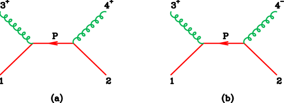
Figure 1: Diagrams for BCFW recursion for $A_{4}(\bm{1},3_{g},4_{g},\bm{2}_{{\bar{Q}}})$

We can now calculate the one quark pair + two gluon amplitudes using the 3-parton amplitudes given in Eqs. (12), (13) by BCFW recursion. As usual for the choice of the BCFW shift momentum,

$$|\hat{j}]=|j]-z|i],\quad\quad|\hat{i}>=|i\rangle+z|j\rangle,$$ (20)

the helicities of the marked particles can take the values, $(h_{i},h_{j})=(+,-),(+,+),(-,-)$ but not $(h_{i},h_{j})=(-,+)$, in order that the amplitude as a function of $z$ vanishes as $z\to\infty$ Britto:2005fq . The four-parton amplitudes are then obtained from,

$$A_{4}(\bm{1}_{Q},3_{g},4_{g},\bm{2}_{{\bar{Q}}})=A_{3}(\bm{1},\hat{3}_{g},-\bm{P})\,\frac{i}{\left\langle 3|\bm{1}|3\right]}\,A_{3}(\bm{P},\hat{4}_{g},\bm{2}_{{\bar{Q}}})\,.$$ (21)

The relevant diagram for the calculation of $A_{4}(\bm{1}_{Q},3_{g}^{+},4_{g}^{+},\bm{2}_{{\bar{Q}}})$ is shown in Fig. 1(a). Taking $i=3$ and $j=4$ we have,

$$|\hat{3}\rangle=|3\rangle+z|4\rangle\,,\quad\quad|\hat{4}]=|4]-z|3]\,,\quad\quad P=p_{1}+\hat{p}_{3}\,.$$ (22)

The onshell condition on the intermediate quark line $P^{2}-m^{2}=\left[3|\bm{1}|\hat{3}\right\rangle=0$ determines that,

$$z=-\frac{\left[3|\bm{1}|3\right\rangle}{\left[3|\bm{1}|4\right\rangle}\,,\quad\quad\langle x\hat{3}\rangle=\frac{\left[3|\bm{1}|x\right\rangle}{\left[3|\bm{1}|4\right\rangle}\langle 43\rangle\,,\quad\quad\left[x\hat{4}\right]=\frac{\left[x|(3+4)|\bm{1}|3\right]}{\left[3|\bm{1}|4\right\rangle}=-\frac{\left[x|(\bm{1}+\bm{2})|\bm{1}|3\right]}{\left[3|\bm{1}|4\right\rangle}\,.$$ (23)

From Eq. (12) using Eq. (4) we have that,

$$A_{3}(\bm{1},\hat{3}^{+}_{g},-\bm{P}) = -i\frac{\langle{\bm{1}|-\bm{P}}\rangle\left\langle q|\bm{1}|3\right]}{m\langle q\hat{3}\rangle}=-i\frac{\langle\bm{1}\bm{P}\rangle\left\langle 4|\bm{1}|3\right]}{m\langle 34\rangle}\,,$$ (24)

$$A_{3}(\bm{P},\hat{4}^{+}_{g},\bm{2}_{{\bar{Q}}}) = i\frac{\langle\bm{P}\bm{2}\rangle\left\langle q|\bm{2}|\hat{4}\right]}{m\langle q4\rangle}=-i\frac{\langle\bm{P}\bm{2}\rangle\left\langle 3|\bm{2}|(\bm{1}+\bm{2})|\bm{1}|3\right]}{m\langle 34\rangle\left[3|\bm{1}|4\right\rangle}=-i\frac{\langle\bm{P}\bm{2}\rangle\left[34\right]m}{\left[3|\bm{1}|4\right\rangle}\,.$$ (25)

For clarity, when a momentum has a negative sign we introduce an additional vertical line in the spinor products, e.g. $\langle ij\rangle=\langle i|j\rangle$. Therefore the answer by BCFW is,

$$-iA_{4}(\bm{1}_{Q},3_{g}^{+},4_{g}^{+},\bm{2}_{{\bar{Q}}})=-\frac{\left[34\right]}{\langle 34\rangle}\frac{1}{\left\langle 3|\bm{1}|3\right]}\langle\bm{1}\bm{P}\rangle\langle\bm{P}\bm{2}\rangle=m\frac{\left[34\right]}{\langle 34\rangle}\frac{1}{\left\langle 3|\bm{1}|3\right]}\langle\bm{1}\bm{2}\rangle\,,$$ (26)

where we have used the relation, c.f. Eq. (3),

$$\langle\bm{1}\bm{P}\rangle\langle\bm{P}\bm{2}\rangle=\langle{\bm{1}^{J}|\bm{P}_{I}}\rangle\langle\bm{P}^{I}\bm{2}_{K}\rangle=-m\langle\bm{1}^{J}\bm{2}_{K}\rangle\,.$$ (27)

For the calculation of $A_{4}(\bm{1}_{Q},3_{g}^{+},4_{g}^{-},\bm{2}_{{\bar{Q}}})$, shown in Fig. 1(b), we use the same shift and require the amplitude,

$$A_{3}(\bm{P},\hat{4}^{-}_{g},\bm{2}_{{\bar{Q}}}) = -i\frac{(\langle\bm{P}4\rangle\left[q\bm{2}\right]+\left[\bm{P}q\right]\langle 4\bm{2}\rangle)}{\left[\hat{4}q\right]}=-i\frac{(\langle\bm{P}4\rangle\left[3\bm{2}\right]+\left[\bm{P}3\right]\langle 4\bm{2}\rangle)}{\left[43\right]}\,.$$ (28)

Therefore the answer by BCFW is

$$-iA_{4}(\bm{1}_{Q},3_{g}^{+},4_{g}^{-},\bm{2}_{{\bar{Q}}}) = -\frac{\left\langle 4|\bm{1}|3\right]}{m\left\langle 3|\bm{1}|3\right]s_{34}}\langle\bm{1}\bm{P}\rangle(\langle\bm{P}4\rangle\left[3\bm{2}\right]+\left[\bm{P}3\right]\langle 4\bm{2}\rangle)$$ (29)

$$= \frac{\left\langle 4|\bm{1}|3\right]}{\left\langle 3|\bm{1}|3\right]s_{34}}(\langle\bm{1}4\rangle\left[3\bm{2}\right]+\left[\bm{1}3\right]\langle 4\bm{2}\rangle)\,,$$

where we have used Eq. (27) with a suitable choice of arguments. Additionally we have $|\bm{p}_{I}\rangle_{\alpha}[\bm{p}^{I}|_{{\dot{\beta}}}=-p_{\alpha{\dot{\beta}}}$, (see Appendix A) so that,

$$\langle\bm{1}\bm{P}\rangle\left[\bm{P}3\right]=\langle{\bm{1}^{J}\bm{P}_{I}\rangle\,[\bm{P}^{I}}{3}]=-\left\langle\bm{1}^{J}|\bm{P}|3\right]=-m\left[\bm{1}^{J}3\right]\,.$$ (30)

Summarizing, the two primitive leading-color amplitudes are given by,

$$-iA_{4}(\bm{1}_{Q},3_{g}^{+},4^{+}_{g},\bm{2}_{{\bar{Q}}}) = m\frac{\left[34\right]}{\langle 34\rangle}\frac{\langle\bm{1}\bm{2}\rangle}{(s_{13}-m^{2})}\,,$$ (31)

$$-iA_{4}(\bm{1}_{Q},3_{g}^{+},4^{-}_{g},\bm{2}_{{\bar{Q}}}) = \frac{\left\langle 4|\bm{1}|3\right]\big{(}[\bm{1}3]\langle 4\bm{2}\rangle+\langle\bm{1}4\rangle[3\bm{2}]\big{)}}{(s_{13}-m^{2})s_{34}}\,.$$ (32)

From Eqs. (31,32) the remaining helicity combinations can be obtained by charge conjugation and line reversal,

$$-iA_{4}(\bm{1}_{Q},3_{g}^{-},4^{-}_{g},\bm{2}_{{\bar{Q}}}) = iA_{4}(\bm{2}_{Q},4_{g}^{+},3^{+}_{g},\bm{1}_{{\bar{Q}}})|_{\langle\rangle\leftrightarrow\left[\right]}=m\frac{\langle 34\rangle}{\left[34\right]}\frac{\left[\bm{1}\bm{2}\right]}{(s_{13}-m^{2})}\,,$$

$$-iA_{4}(\bm{1}_{Q},3_{g}^{-},4^{+}_{g},\bm{2}_{{\bar{Q}}}) = iA_{4}(\bm{2}_{Q},4_{g}^{+},3^{-}_{g},\bm{1}_{{\bar{Q}}})=\frac{\langle 3|\bm{1}|4]\big{(}\langle\bm{1}3\rangle[4\bm{2}]+[\bm{1}4]\langle 3\bm{2}\rangle\big{)}}{(s_{13}-m^{2})s_{34}}\,.$$ (33)

The amplitudes in Eqs. (31,32) and (33) clearly satisfy the BCJ relation,

$$(s_{13}-m^{2})A_{4}(\bm{1}_{Q},3_{g},4_{g},\bm{2}_{{\bar{Q}}})=(s_{14}-m^{2})A_{4}(\bm{1}_{Q},4_{g},3_{g},\bm{2}_{{\bar{Q}}})\,.$$ (34)

The subleading color amplitudes can be obtained from Eq. (33) using the relation Eq. (19). Applying Eq. (19) and simplifying we have,

$$-iA_{4}(\bm{1}_{Q},3^{+}_{g},\bm{2}_{{\bar{Q}}},4_{g}^{+}) = m\frac{\left[34\right]^{2}\langle\bm{1}\bm{2}\rangle}{(s_{13}-m^{2})(s_{14}-m^{2})}\,,$$

$$-iA_{4}(\bm{1}_{Q},3_{g}^{-},\bm{2}_{{\bar{Q}}},4_{g}^{+}) = -\frac{\langle 3|\bm{1}|4]\big{(}\langle\bm{1}3\rangle[4\bm{2}]+[\bm{1}4]\langle 3\bm{2}\rangle\big{)}}{(s_{13}-m^{2})(s_{14}-m^{2})}\,.$$ (35)

4.2 Two quark pair amplitude

4.2.1 Color algebra

We now write down the amplitude for 4 quarks, where 1 and 2 have mass $m$, and 3 and 4 are massless,

$${\cal A}_{4}(\bm{1}_{x_{1}},\bm{2}_{x_{2}},3_{x_{3}}^{h_{3}},4_{x_{4}}^{h_{4}})=g^{2}(t^{C})_{x_{1},x_{2}}\,(t^{C})_{x_{3},x_{4}}\;A_{4}(\bm{1}_{Q},\bm{2}_{{\bar{Q}}},3_{q}^{h_{3}},4_{\bar{q}}^{h_{4}})\,.$$ (36)

The result for the amplitude squared summed over colors is,

$$\sum_{x_{1},x_{2},x_{3},x_{4}}|{\cal A}_{4}(\bm{1}_{x_{1}},\bm{2}_{x_{2}},3^{h_{3}}_{x_{3}},4^{h_{4}}_{x_{4}})|^{2}=g^{4}V\,\big{|}A_{4}(\bm{1}_{Q},\bm{2}_{{\bar{Q}}},3_{q}^{h_{3}},4_{\bar{q}}^{h_{4}})\big{|}^{2}\,.$$ (37)

4.2.2 Result for two quark pair amplitude

The result for two quark pair amplitude is simply given by,

$$-iA_{4}(\bm{1}_{Q},\bm{2}_{{\bar{Q}}},3_{q}^{-},4_{\bar{q}}^{+})=\frac{\langle\bm{1}3\rangle\left[4\bm{2}\right]+\left[\bm{1}4\right]\langle 3\bm{2}\rangle}{s_{34}}\,.$$ (38)

The primitive amplitude with opposite helicities of the massless quarks is obtained by exchanging labels 3 and 4.

5 Example of BCFW recursion

In this section we illustrate the calculation of the 5-parton amplitude using BCFW recursion exploiting the amplitudes presented in sections 3 and 4. As an example we calculate one of the amplitudes for one massive quark pair, one massless quark pair and a gluon, ${\cal A}_{5}(\bm{1},\bm{2}_{{\bar{Q}}},3_{q}^{-},4_{\bar{q}}^{+},5_{g}^{+})$. For the BCFW shift we take $i=5,j=4$ so that,

$$|\hat{5}\rangle\equiv|5\rangle+z\,|4\rangle,\;\;\;\;|\hat{4}]\equiv|4]-z\,|5]$$ (39)

5.1 Residue at $z_{15}$

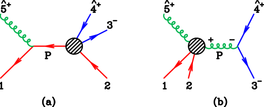
Figure 2: Diagrams for BCFW recursion for $A(\bm{1}_{Q},\bm{2}_{{\bar{Q}}},3_{q}^{-},4_{\bar{q}}^{+},5_{g}^{+})$

For the diagram in Fig. 2(a) we have that,

$$\left.A_{5}(\bm{1}_{Q},\bm{2}_{{\bar{Q}}},3_{q}^{-},4_{\bar{q}}^{+},5_{g}^{+})\right|_{z_{15}}=-A_{3}(\bm{1}_{Q},\hat{5}^{+}_{g},-\bm{P}_{{\bar{Q}}})\frac{i}{\left\langle 5|\bm{1}|5\right]}A_{4}(\bm{P}_{Q},\bm{2}_{{\bar{Q}}},3_{q}^{-},\hat{4}_{\bar{q}}^{+})\,,$$ (40)

where $P=p_{1}+\hat{p}_{5}$ and the overall sign is due to the definition of the color decomposition, see Eq. (73). For $i=5$ and $j=4$ the onshell condition for the massive intermediate quark is $\langle 5|\bm{1}|5]+z_{15}\langle 4|\bm{1}|5]=0$. The shifted spinors are,

$$\!\!\!z_{15}=-\frac{\langle 5|\bm{1}|5]}{\langle 4|\bm{1}|5]}\,,\quad~{}\,|\hat{5}\rangle=-\frac{|\bm{1}|5|4\rangle}{[5|\bm{1}|4\rangle},\quad~{}\,|{\hat{4}}]\!=\frac{|(4+5)|\bm{1}|5]}{\langle 4|\bm{1}|5]}\,.$$ (41)

For the amplitude on the left hand side of Fig. 2(a) we use the expression given in Eq. (12) with Eq. (4) and we choose $\langle q|=\langle 4|$. For the amplitude on the right hand side of Fig. 2(a) we use Eq. (38),

$$A_{3}(\bm{1}_{Q},\hat{5}^{+}_{g},-\bm{P}_{{\bar{Q}}}) = -i\frac{\langle\bm{1}|-\bm{P}\rangle\left\langle q|\bm{1}|5\right]}{m\langle q\hat{5}\rangle}=i\frac{\langle\bm{1}\bm{P}\rangle\left\langle 4|\bm{1}|5\right]}{m\langle 45\rangle}$$ (42)

$$A_{4}(\bm{P}_{Q},\bm{2}_{{\bar{Q}}},3_{q}^{-},\hat{4}_{\bar{q}}^{+}) = i\frac{(\langle\bm{P}3\rangle\left[\hat{4}\bm{2}\right]+\left[\bm{P}\hat{4}\right]\langle 3\bm{2}\rangle)}{s_{3\hat{4}}}=i\frac{(\left[\bm{P}\hat{4}\right]\langle 3\bm{2}\rangle-\langle\bm{P}3\rangle\left[\bm{2}\hat{4}\right])}{\langle 43\rangle\left[3\hat{4}\right]}$$ (43)

$$= i\frac{(\left[\bm{P}|(4+5)|\bm{1}|5\right]\langle 3\bm{2}\rangle-\langle\bm{P}3\rangle\left[\bm{2}|(4+5)|\bm{1}|5\right])}{\langle 43\rangle\left[3|(4+5)|\bm{1}|5\right]}$$ (44)

Now using the relations for massive spinors in Eq. (3),

$$\langle\bm{1}\bm{P}\rangle\langle\bm{P}x\rangle = \langle\bm{1}^{J}\bm{P}_{I}\rangle\langle\bm{P}^{I}x\rangle=-m\langle\bm{1}^{J}x\rangle\,,$$

$$\langle\bm{1}\bm{P}\rangle\left[\bm{P}x\right] = \langle\bm{1}^{J}\bm{P}_{I}\rangle\left[\bm{P}^{I}x\right]=-\left\langle\bm{1}^{J}|\bm{P}|x\right]$$ (45)

we thus have,

$$\langle\bm{1}\bm{P}\rangle\left[\bm{P}|(4+5)|\bm{1}|5\right] = -\left\langle\bm{1}|(\bm{1}+\hat{5})|(4+5)|\bm{1}|5\right]$$ (46)

$$= -m\left[\bm{1}|(4+5)|\bm{1}|5\right]-\langle\bm{1}\hat{5}\rangle\left[5|(4+5)|\bm{1}|5\right]$$

$$= m\left[5|\bm{1}|(4+5)|\bm{1}\right]+m\left[\bm{1}|5|4\right\rangle\left[54\right]$$

Hence,

$$\frac{\langle\bm{1}\bm{P}\rangle}{m}A_{4}(\bm{P}_{Q},\bm{2}_{{\bar{Q}}},3_{q}^{-},\hat{4}_{\bar{q}}^{+}) = i\Big{(}\big{(}\left[5|\bm{1}|(4+5)|\bm{1}\right]+\left[\bm{1}|5|4\right\rangle\left[54\right]\big{)}\langle 3\bm{2}\rangle+\langle\bm{1}3\rangle\left[\bm{2}|(4+5)|\bm{1}|5\right]\Big{)}$$ (47)

$$\times \frac{1}{\langle 43\rangle\left[3|(4+5)|\bm{1}|5\right]}\,.$$

So the final result is,

$$A_{5}(\bm{1}_{Q},\bm{2}_{{\bar{Q}}},3_{q}^{-},4_{\bar{q}}^{+},5_{g}^{+})\big{|}_{z_{15}} = \frac{i}{\left\langle 5|\bm{1}|5\right]}\frac{\left\langle 4|\bm{1}|5\right]}{\langle 45\rangle}\frac{1}{\langle 43\rangle\left[3|(4+5)|\bm{1}|5\right]}$$

$$\times \Big{(}\big{(}\left[5|\bm{1}|(4+5)|\bm{1}\right]+\left[\bm{1}5\right]\langle 54\rangle\left[54\right]\big{)}\langle 3\bm{2}\rangle+\langle\bm{1}3\rangle\left[\bm{2}|(4+5)|\bm{1}|5\right]\Big{)}$$

$$= \frac{i}{\left\langle 5|\bm{1}|5\right]}\frac{\left\langle 4|\bm{1}|5\right]}{\langle 45\rangle}\frac{1}{\langle 34\rangle\left[3|(4+5)|\bm{1}|5\right]}$$

$$\times \Big{(}\big{(}\left[\bm{1}|(4+5)|\bm{1}|5\right]+\left[\bm{1}5\right]\langle 45\rangle\left[54\right]\big{)}\langle 3\bm{2}\rangle+\langle\bm{1}3\rangle\left[5|\bm{1}|(4+5)|\bm{2}\right]\Big{)}$$

5.2 Residue at $z_{34}$

For the second diagram, Fig. 2(b),

$$\left.A_{5}(\bm{1}_{Q},\bm{2}_{{\bar{Q}}},3_{q}^{-},4_{\bar{q}}^{+},5_{g}^{+})\right|_{z_{34}}=-A_{4}(\bm{1}_{Q},\hat{5}^{+}_{g},P_{g}^{+},\bm{2}_{{\bar{Q}}})\frac{-i}{s_{34}}A_{3}(3_{q}^{-},-P_{g}^{-},\hat{4}_{\bar{q}}^{+})\,,$$ (49)

where $P=p_{3}+\hat{p}_{4}$ and overall sign is because of the definition of the color amplitude. For $i=5$ and $j=4$ the onshell condition for the intermediate gluon line is $(\left[34\right]-z_{34}\left[35\right])\langle 43\rangle=0$. The shifted spinors in this case are,

$$\!\!\!z_{34}=\frac{\left[34\right]}{\left[35\right]}\,,\quad|\hat{5}\rangle=-\frac{|(4+5)|3]}{\left[35\right]}\,,\quad|{\hat{4}}]=|3]\frac{\left[45\right]}{\left[35\right]},\quad~{}\,\langle P|=-\frac{[5|(3+4)|}{\left[35\right]}\,,\quad|P]=|3]\,.$$ (50)

Inserting the amplitudes from Eqs. (31) and (13) gives,

$$A_{4}(\bm{1}_{Q},\hat{5}^{+}_{g},P_{g}^{+},\bm{2}_{{\bar{Q}}}) = im\frac{\left[P5\right]}{\langle P\hat{5}\rangle}\frac{\langle\bm{1}\bm{2}\rangle}{\left[5|\bm{1}|\hat{5}\right\rangle}=-im\frac{\left[35\right]^{2}}{s_{345}}\frac{\langle\bm{1}\bm{2}\rangle\left[35\right]}{\left[3|(4+5)|\bm{1}|5\right]}\,$$ (51)

$$A_{3}(3_{q}^{-},-P_{g}^{-},\hat{4}_{\bar{q}}^{+}) = (-i)\frac{\langle 3|-\!P\rangle\left[q\hat{4}\right]}{\left[-Pq\right]}=i\frac{\langle 3P\rangle\left[54\right]}{\left[P5\right]}=-i\frac{\langle 34\rangle\left[45\right]^{2}}{\left[35\right]^{2}}\,.$$ (52)

since,

$$\left[P5\right]=\left[35\right]\,,\quad\quad\langle P\hat{5}\rangle=\frac{\left[5|(3+4)|(4+5)|3\right]}{\left[35\right]^{2}}=-\frac{s_{345}}{\left[35\right]}\,,\quad\quad\left[5|\bm{1}|\hat{5}\right\rangle=\frac{\left[3|(4+5)|\bm{1}|5\right]}{\left[35\right]}$$ (53)

Inserting the results from Eqs. (51) and (52) gives,

$$A_{5}(\bm{1}_{Q},\bm{2}_{{\bar{Q}}},3_{q}^{-},4_{\bar{q}}^{+},5_{g}^{+})\big{|}_{z_{34}} = (-1)\times(-im)\frac{\left[35\right]^{2}}{s_{345}}\frac{\langle\bm{1}\bm{2}\rangle\left[35\right]}{\left[3|(4+5)|\bm{1}|5\right]}\times\frac{i}{\langle 34\rangle\left[34\right]}\times(-i)\frac{\langle 34\rangle\left[45\right]^{2}}{\left[35\right]^{2}}$$ (54)

$$= i\frac{m\left[35\right]\left[45\right]^{2}}{s_{345}}\frac{\langle\bm{1}\bm{2}\rangle}{\left[34\right]\left[3|(4+5)|\bm{1}|5\right]}$$

The diagram in Fig. 2(b) with the opposite helicity of gluon exchanged vanishes, because the amplitude on the right hand side is proportional to,

$$A_{3}(3_{q}^{-},-P_{g}^{+},4_{\bar{q}}^{+})=i\frac{\langle 3q\rangle[\hat{4}|{-P}]}{\langle{-P}|q\rangle}$$ (55)

and from Eq. (50) both $[\hat{4}|$ and $|-P]$ are proportional to $|3]$. Thus the sum of the two contributions given in Eqs. (LABEL:eq:bcfwres1) and (54) gives the total result for $A_{5}(\bm{1}_{Q},\bm{2}_{{\bar{Q}}},3_{q}^{-},4_{\bar{q}}^{+},5_{g}^{+})$,

$$-iA_{5}(\bm{1}_{Q},\bm{2}_{{\bar{Q}}},3^{-}_{q},4^{+}_{\bar{q}},5^{+}_{g}) = \frac{1}{\left[3|(4+5)|\bm{1}|5\right]}\*\Big{[}\frac{m\*\langle\bm{1}\bm{2}\rangle\*\left[35\right]\*\left[45\right]^{2}}{s_{345}\*\left[34\right]}$$

$$+ \frac{1}{\left\langle 5|\bm{1}|5\right]}\*\frac{\left\langle 4|\bm{1}|5\right]}{\langle 45\rangle\*\langle 34\rangle}\*\Big{(}\langle\bm{1}3\rangle\*\left[5|\bm{1}|(4+5)|\bm{2}\right]+\left[\bm{1}|(4+5)|\bm{1}|5\right]\*\langle 3\bm{2}\rangle+\left[\bm{1}5\right]\*\langle 3\bm{2}\rangle\*s_{45}\Big{)}\Big{]}\,.$$

We note that, at this stage, the amplitude appears to contain an unphysical pole represented by the overall factor $\left[3|(4+5)|\bm{1}|5\right]$. This is also the case for the result given in ref. Lazopoulos:2021mna , which is presented in a slightly different form but with which this agrees (after taking the limit in which one quark pair is massless). By using the equations of motion and applying Schouten identities one can demonstrate explicitly that this pole is not present. The result for this amplitude presented below in section 6 has been simplified in this way.

6 Five parton amplitudes

6.1 One quark pair + 3 gluon amplitudes

6.1.1 Color algebra

The general color decomposition is given by Eq. (17). For $n=5$ we have,

$${\cal A}_{5}(\bm{1}_{x_{1}},3_{C_{3}},4_{C_{4}},5_{C_{5}},\bm{2}_{x_{2}})\ =\ g^{3}\sum_{\sigma\in S_{3}}(t^{C_{\sigma(3)}}t^{C_{\sigma(4)}}t^{C_{\sigma(5)}})_{x_{1}x_{2}}A_{5}(\bm{1}_{Q},\sigma(3)_{g},\sigma(4)_{g},\sigma(5)_{g},\bm{2}_{{\bar{Q}}})\ ,$$ (57)

Squaring the amplitude and summing over colors we obtain the following expression Mangano:1987kp ,

$$\sum_{\rm colors}|{\cal A}(\bm{1}_{x_{1}},3_{C_{3}},4_{C_{5}},5_{C_{5}},\bm{2}_{x_{2}})|^{2}=g^{6}\,\frac{(N^{2}-1)}{N^{2}}\sum_{j=0}^{2}N^{2j}\sum_{\sigma\in S_{3}}\,H_{j}(3,4,5)\,.$$ (58)

Introducing the compact notation,

$$(3,4,5)=A_{5}(\bm{1}_{Q},3_{g},4_{g},5_{g},\bm{2}_{{\bar{Q}}})$$ (59)

we get

$$H_{2}(3,4,5) = |(3,4,5)|^{2}\,,$$ (60)

$$H_{1}(3,4,5) = -(3,4,5)^{*}\,[2(3,4,5)+(3,5,4)+(4,3,5)-(5,4,3)]\,,$$ (61)

$$H_{0}(3,4,5) = (3,4,5)^{*}\sum_{\sigma\in S_{3}}(i,j,k)\,.$$ (62)

Note that ref. Mangano:1987kp contains a typographical error in the sign of the final term in the expression for $H_{1}(3,4,5)$ which we have corrected in Eq. (61).

6.2 Results for one quark pair + 3 gluon amplitudes

The amplitude with gluons of all positive helicity is taken directly from ref. Ochirov:2018uyq ,

$$-iA_{5}(\bm{1},3_{g}^{+},4_{g}^{+},5_{g}^{+},\bm{2})=-m\*\frac{\left[45\right]\*\left\langle 4|\bm{1}|3\right]+\left\langle 3|\bm{1}|3\right]\*\left[35\right]}{\langle 34\rangle\*\langle 45\rangle}\*\frac{\langle\bm{1}\bm{2}\rangle}{\left\langle 3|\bm{1}|3\right]\*\left\langle 5|\bm{2}|5\right]}\,.\\$$ (63)

The amplitude for gluon 3 of negative helicity is also given in ref. Ochirov:2018uyq . However it contains an unphysical pole that can, with suitable application of Schouten identities and momentum conservation, be removed. The final simplified result is,

$$-iA_{5}(\bm{1},3_{g}^{-},4_{g}^{+},5_{g}^{+},\bm{2})=\frac{1}{\langle 34\rangle\*\langle 45\rangle\*\left\langle 3|\bm{1}|3\right]\*\left\langle 5|\bm{2}|5\right]}$$ (64)

$$\times \Bigg{\{}\Bigg{[}\frac{m\*\langle 34\rangle\*\left[45\right]\*\big{(}\left\langle 3|\bm{1}|4\right]\*s_{345}-\left\langle 3|\bm{1}|3\right]\*\left[45\right]\*\langle 53\rangle\big{)}}{s_{345}\*\left[34\right]}-\frac{\left\langle 3|\bm{1}|(4+5)|3\right\rangle\*\left\langle 3|\bm{2}|5\right]\*\left\langle 3|1|3\right]}{m\*s_{345}}\Bigg{]}\*\langle\bm{1}\bm{2}\rangle$$

$$+ \frac{\big{(}\left\langle 3|\bm{2}|5\right]\*\left\langle 3|\bm{1}|3\right]-m^{2}\*\langle 34\rangle\*\left[45\right]\big{)}}{m}\*\langle\bm{1}3\rangle\*\langle 3\bm{2}\rangle\Bigg{\}}\,.$$

The position of the negative helicity gluon can be moved to the other end of the string through the line-reversal relation,

$$A_{5}(\bm{1}_{q},3_{g}^{+},4_{g}^{+},5_{g}^{-},\bm{2}_{\bar{q}})=A_{5}(\bm{2}_{q},5_{g}^{-},4_{g}^{+},3_{g}^{+},\bm{1}_{{\bar{Q}}})\,.$$ (65)

The final amplitude we need, with the negative helicity gluon in the middle of the string, is fixed by the previous two equations through the BCJ relation,

$$(s_{13}+s_{34}-m^{2})\,A_{5}(\bm{1}_{Q},4_{g}^{+},3_{g}^{-},5_{g}^{+},\bm{2}_{{\bar{Q}}}) =$$

$$(s_{23}-m^{2})\,A_{5}(\bm{1}_{Q},4_{g}^{+},5_{g}^{+},3_{g}^{-},\bm{2}_{{\bar{Q}}})-(s_{13}-m^{2})\,A_{5}(\bm{1}_{Q},3_{g}^{-},4_{g}^{+},5_{g}^{+},\bm{2}_{{\bar{Q}}})\,.$$ (66)

Forming the appropriate combination and manipulating to remove the spurious pole we find,

$$-iA_{5}(\bm{1}_{q},3_{g}^{+},4_{g}^{-},5_{g}^{+},\bm{2}_{\bar{q}})=\frac{\langle\bm{1}4\rangle\*\langle 4\bm{2}\rangle\*\left\langle 4|\bm{1}|3\right]\*\left\langle 4|\bm{2}|5\right]}{m\*\langle 34\rangle\*\langle 45\rangle\*\left\langle 3|\bm{1}|3\right]\*\left\langle 5|\bm{2}|5\right]}$$ (67)

$$+ \frac{\langle\bm{1}\bm{2}\rangle}{\langle 35\rangle\*\left\langle 3|\bm{1}|3\right]\*\left\langle 5|\bm{2}|5\right]\*s_{345}}\*\Big{(}m\*\frac{\left[35\right]}{\left[45\right]}\*\Big{[}\langle 43\rangle\*\left[35\right]\*\left\langle 4|\bm{2}|4\right]-s_{345}\*\left\langle 4|\bm{2}|5\right]\Big{]}-\frac{\left\langle 4|\bm{1}|3\right]\*\left\langle 4|\bm{2}|4\right]\*\left\langle 4|\bm{1}|\bm{2}|4\right\rangle}{m\*\langle 45\rangle}\Big{)}$$

$$+ \frac{\langle\bm{1}\bm{2}\rangle}{\langle 35\rangle\*\left\langle 5|\bm{2}|5\right]\*s_{345}}\*\Big{(}\frac{m\*\langle 35\rangle\*\left[35\right]^{3}}{\left[43\right]\*\left[45\right]}+\frac{\left\langle 4|\bm{1}|\bm{2}|4\right\rangle^{2}}{m\*\langle 43\rangle\*\langle 45\rangle}\Big{)}\,.$$

The remaining amplitudes are obtained through a simple operation,

$$A_{5}(\bm{1},3_{g}^{-h_{3}},4_{g}^{-h_{4}},5_{g}^{-h_{5}},\bm{2})=-A_{5}(\bm{1},3_{g}^{h_{3}},4_{g}^{h_{4}},5_{g}^{h_{5}},\bm{2})|_{\langle\rangle\leftrightarrow\left[\right]}\,,$$ (68)

in an obvious notation where $\langle\rangle\leftrightarrow\left[\right]$ denotes the interchange of angle and square brackets.

6.3 Two quark pairs and one gluon

6.3.1 Color algebra for two quark pairs and one gluon

In the case of two quark pairs and one gluon the possible color structures are the following,

$${\cal A}_{5}(\bm{1}_{x_{1}},\bm{2}_{x_{2}},3_{x_{3}},4_{x_{5}},5_{C_{5}}) = g^{3}\Big{(}-(t^{C_{5}})_{x_{1}x_{4}}\delta_{x_{3}x_{2}}A^{(1)}-(t^{C_{5}})_{x_{3}x_{2}}\delta_{x_{1}x_{4}}A^{(2)}$$ (69)

$$- \frac{1}{N}(t^{C_{5}})_{x_{1}x_{2}}\delta_{x_{3}x_{4}}A^{(3)}-\frac{1}{N}(t^{C_{5}})_{x_{3}x_{4}}\delta_{x_{1}x_{2}}A^{(4)}\Big{)}\,.$$

Squaring and summing over colors we find ($V=N^{2}-1$)

$$\sum_{\rm colors}|{\cal A}_{5}(\bm{1}_{x_{1}},\bm{2}_{x_{2}},3_{x_{3}},4_{x_{5}},5_{C_{5}})|^{2} = \frac{V}{N}\Big{[}(N^{2}-1)\*\left(|A^{(1)}|^{2}+|A^{(2)}|^{2}\right)$$ (70)

$$-A^{(1)}A^{(2)*}-A^{(2)}A^{(1)*}-A^{(3)}A^{(4)*}-A^{(4)}A^{(3)*}$$

$$+|A^{(1)}+A^{(2)}+A^{(3)}+A^{(4)}|^{2}\Big{]}\,.$$

Note that the term on the final line will not contribute since this combination of subamplitudes is identically zero. Imposing this condition we obtain,

$$\sum_{\rm colors}|{\cal A}_{5}(\bm{1}_{x_{1}},\bm{2}_{x_{2}},3_{x_{3}},4_{x_{5}},5_{C_{5}})|^{2} = VN\,\Big{[}|A^{(1)}|^{2}+|A^{(2)}|^{2}$$ (71)

$$+ \frac{1}{N^{2}}\Big{(}|A^{(3)}|^{2}+|A^{(4)}|^{2}-2\big{|}(A^{(1)}+A^{(2)})\big{|}^{2}\Big{)}\Big{]}\,.$$

Using the Melia basis, as described in ref. Johansson:2015oia , this should be written in terms of three independent primitives as,

$${\cal A}_{5}(\bm{1}_{x_{1}},\bm{2}_{x_{2}},3_{x_{3}},4_{x_{5}},5_{C_{5}}) = g^{3}\Big{(}A_{12345}\,C_{12345}+A_{12354}\,C_{12354}+A_{12534}\,C_{12534}\Big{)}\,,$$ (72)

where the color coefficients are given by,

$$C_{12345} = -(t^{C_{5}}t^{D})_{x_{1}x_{2}}(t^{D})_{x_{3}x_{4}}$$

$$C_{12534} = -(t^{D}t^{C_{5}})_{x_{1}x_{2}}(t^{D})_{x_{3}x_{4}}$$

$$C_{12354} = -(t^{C_{5}}t^{D})_{x_{1}x_{2}}(t^{D})_{x_{3}x_{4}}-(t^{D})_{x_{1}x_{2}}(t^{D}t^{C_{5}})_{x_{3}x_{4}}\,.$$ (73)

Performing the color algebra and comparing we can thus identify,

$$A^{(1)} = A_{12345},\;A^{(2)}=A_{12534},\;A^{(3)}=-A_{12345}-A_{12354}-A_{12534},\;A^{(4)}=A_{12354}$$ (74)

These clearly satisfy the constraint alluded to above,

$$A^{(1)}+A^{(2)}+A^{(3)}+A^{(4)}=0\,.$$ (75)

6.3.2 BCJ relations

We can further reduce the set of primitives by using the kinematic-algebra basis that also accounts for BCJ relations between the amplitudes. In that case we fix quark 3 to be in position 3 and find the result in terms of two amplitudes,

$$p_{2}\cdot p_{5}\;A_{12534}-p_{1}\cdot p_{5}\;A_{12345}-p_{14}\cdot p_{5}\;A_{12354}=0\,,$$ (76)

$${\cal A}_{5}(\bm{1}_{x_{1}},\bm{2}_{x_{2}},3_{x_{3}},4_{x_{4}},5_{C_{5}}) = g^{3}\bigg{[}A_{12345}\Big{(}C_{12345}+C_{12534}\,\frac{p_{1}\cdot p_{5}}{p_{2}\cdot p_{5}}\Big{)}$$ (77)

$$\;\;+A_{12354}\Big{(}C_{12354}+C_{12534}\,\frac{p_{14}\cdot p_{5}}{p_{2}\cdot p_{5}}\Big{)}\bigg{]}\,.$$

6.4 Results for two quark pairs + 1 gluon amplitudes

Manipulating the result derived in the previous section in Eq. (5.2) to remove the unphysical pole, we find the amplitude for a positive helicity gluon,

$$-iA(\bm{1}_{Q},\bm{2}_{{\bar{Q}}},3^{-}_{q},4^{+}_{\bar{q}},5^{+}_{g}) = \frac{1}{m\*\langle 45\rangle}\*\Bigg{[}-\frac{\langle\bm{1}3\rangle\*\langle 3\bm{2}\rangle\*\left\langle 4|\bm{1}|5\right]}{\langle 34\rangle\*\left\langle 5|\bm{1}|5\right]}$$ (78)

$$+ \frac{\langle\bm{1}\bm{2}\rangle}{s_{34}}\*\Big{(}\frac{\left\langle 3|\bm{2}|4\right]\*\left\langle 4|\bm{1}|5\right]}{\left\langle 5|\bm{1}|5\right]}+\frac{\left\langle 3|\bm{2}|(3+5)|4\right\rangle\*\left[45\right]}{s_{345}}\Big{)}\Bigg{]}\,.$$

The corresponding result for a negative helicity gluon after removal of the unphysical pole is,

$$-iA(\bm{1}_{Q},\bm{2}_{{\bar{Q}}},3^{-}_{q},4^{+}_{\bar{q}},5^{-}_{g}) = \frac{1}{m\*\left[45\right]}\*\Bigg{[}-\frac{\left[\bm{1}4\right]\*\left[4\bm{2}\right]\*\left\langle 5|\bm{1}|4\right]}{\left\langle 5|\bm{1}|5\right]\*\left[34\right]}$$ (79)

$$+ \frac{\left[\bm{1}\bm{2}\right]}{s_{34}}\*\Big{(}\frac{\langle 35\rangle\*\left[4|(3+5)|\bm{2}|4\right]}{s_{345}}-\frac{\left\langle 3|\bm{2}|4\right]\*\left\langle 5|\bm{1}|4\right]}{\left\langle 5|\bm{1}|5\right]}\Big{)}\Bigg{]}\,.$$

6.4.1 Relationship to other amplitudes

The other leading color amplitude is related to the one given above through charge conjugation,

$$A(\bm{1}_{Q},\bm{2}_{{\bar{Q}}},5^{-}_{g},3^{-}_{q},4^{+}_{\bar{q}})=A(\bm{2}_{Q},\bm{1}_{{\bar{Q}}},4^{-}_{q},3^{+}_{\bar{q}},5^{+}_{g})\big{.}_{\langle\rangle\leftrightarrow\left[\right]}\,.$$ (80)

The subleading color amplitude $A(\bm{1}_{Q},\bm{2}_{{\bar{Q}}},3_{q},5_{g},4_{\bar{q}})$ can be obtained by forming a combination with amplitudes in which the heavy quark and antiquark are interchanged,

$$A(\bm{1}_{Q},\bm{2}_{{\bar{Q}}},3^{-}_{q},5_{g},4^{+}_{\bar{q}}) = A(\bm{2}_{Q},\bm{1}_{{\bar{Q}}},3^{-}_{q},4^{+}_{\bar{q}},5_{g})+A(\bm{1}_{Q},\bm{2}_{{\bar{Q}}},5_{g},3^{-}_{q},4^{+}_{\bar{q}})\,.$$ (81)

Simplifying this combination we find,

$$-iA_{5}(\bm{1}_{Q},\bm{2}_{{\bar{Q}}},3^{-}_{q},5^{+}_{g},4^{+}_{\bar{q}})=\frac{1}{m\*\langle 35\rangle\*\langle 45\rangle}\*\Bigg{[}\langle\bm{1}\bm{2}\rangle\*\Big{(}\frac{\left\langle 3|1|4\right]}{\left[34\right]}-\frac{\left[45\right]\*\left\langle 5|(3+4)|\bm{1}|3\right\rangle}{\left[34\right]\*s_{345}}\Big{)}-\langle\bm{1}3\rangle\*\langle 3\bm{2}\rangle\Bigg{]}\,.$$ (82)

$$-iA_{5}(\bm{1}_{Q},\bm{2}_{{\bar{Q}}},3^{-}_{q},5^{-}_{g},4^{+}_{\bar{q}})=-\frac{1}{m\*\left[35\right]\*\left[45\right]}\*\Bigg{[}\left[\bm{1}\bm{2}\right]\*\Big{(}\frac{\left\langle 3|1|4\right]}{\langle 34\rangle}-\frac{\langle 35\rangle\*\left[5|(3+4)|\bm{1}|4\right]}{\langle 34\rangle\*s_{345}}\Big{)}+\left[\bm{1}4\right]\*\left[4\bm{2}\right]\Bigg{]}\,.$$ (83)

Together with the identities in Eq. (74), all amplitudes needed to construct the full squared matrix element for this process are at hand.

7 Six parton amplitudes

7.1 One quark pair + 4 gluon amplitudes

7.1.1 Color structure

Here we describe the color structure for one massive quark pair + 4 gluon amplitudes. The form of the expansion into color-ordered primitives is taken from Eq. (17).

$${\cal A}_{6}(1_{x_{1}},3_{C_{3}},4_{C_{4}},5_{C_{5}},6_{C_{6}},2_{x_{2}})\ =\ g^{4}\sum_{\sigma\in S_{4}}(t^{C_{\sigma(3)}}t^{C_{\sigma(4)}}t^{C_{\sigma(5)}}t^{C_{\sigma(6)}})_{x_{1}x_{2}}A_{6}(1_{Q},\sigma(3),\sigma(4),\sigma(5),\sigma(6),2_{{\bar{Q}}})\ ,$$ (84)

where $S_{4}$ is the permutation group on $4$ elements, and $A_{6}$ are the tree-level partial amplitudes.

Squaring the amplitude and summing over colors we obtain the following expression Mangano:1987kp ,

$$\sum_{\rm colors}|{\cal A}_{6}(\bm{1}_{Q},3_{C_{3}},4_{C_{4}},5_{C_{5}},6_{C_{6}},\bm{2}_{{\bar{Q}}})|^{2}=g^{8}\,\frac{(N^{2}-1)}{N^{3}}\sum_{j=0}^{3}\,N^{2j}\sum_{\sigma\in S_{4}}\,H_{j}(3,4,5,6)\,.$$ (85)

Introducing the compact notation for the color-ordered primitives $A$,

$$(3,4,5,6)=A_{6}(\bm{1}_{Q},3_{g},4_{g},5_{g},6_{g},\bm{2}_{{\bar{Q}}})$$ (86)

we get,

$$H_{3}(3,4,5,6) = |(3,4,5,6)|^{2},$$

$$H_{2}(3,4,5,6) = (3,4,5,6)^{*}\,[-3(3,4,5,6)-(3,4,6,5)-(3,5,4,6)$$

$$- (4,3,5,6)+(3,6,5,4)+(5,4,3,6)+(5,6,3,4)$$

$$+ (5,6,4,3)+(6,4,5,3)+(6,5,3,4)],$$

$$H_{1}(3,4,5,6) = (3,4,5,6)^{*}\,[M(3,4,5,6)-M(6,5,4,3)]$$

$$M(3,4,5,6) = 3(3,4,5,6)+2(3,4,6,5)+2(3,5,4,6)+2(4,3,5,6)+(3,5,6,4)$$

$$+ (3,6,4,5)+(4,3,6,5)+(4,5,3,6)+(5,3,4,6),$$

$$H_{0}(3,4,5,6) = -(3,4,5,6)^{*}\,\sum_{\sigma\in S_{4}}(i,j,k,l).$$ (87)

7.1.2 Results for $A_{6}(\bm{1}_{Q},3_{g},4_{g},5_{g},6_{g},\bm{2}_{{\bar{Q}}})$

The all-plus helicity result is taken from Ochirov Ochirov:2018uyq ,

$$-iA(\bm{1}_{Q},3_{g}^{+},4_{g}^{+},5_{g}^{+},6_{g}^{+},\bm{2}_{{\bar{Q}}}) = m\*\langle\bm{1}\bm{2}\rangle\*\frac{[3|\big{(}\hbox to0.0pt{$\;\!\!\not$\hss}{p}_{13}\hbox to0.0pt{$\;\!\!\not$\hss}{p}_{4}+s_{13}-m^{2}\big{)}\*\big{(}\hbox to0.0pt{$\;\!\!\not$\hss}{p}_{134}\hbox to0.0pt{$\;\!\!\not$\hss}{p}_{5}+s_{134}-m^{2})\big{)}|6]}{(\left\langle 3|\bm{1}|3\right]\*(s_{134}-m^{2})\*\left\langle 6|2|6\right]\*\langle 34\rangle\*\langle 45\rangle\*\langle 56\rangle)}$$ (88)

$$= -m\*\langle\bm{1}\bm{2}\rangle\*\frac{m^{2}\*\langle 45\rangle\*\left[34\right]\*\left[56\right]+(s_{134}-m^{2})\*\left[6|(3+4+5)|\bm{1}|3\right]}{(\left\langle 3|\bm{1}|3\right]\*(s_{134}-m^{2})\*\left\langle 6|2|6\right]\*\langle 34\rangle\*\langle 45\rangle\*\langle 56\rangle)}\,.$$

The result with one negative helicity adjacent to the massive quark is also taken from ref Ochirov:2018uyq ,

$$-iA_{6}(\bm{1},3_{g}^{-},4_{g}^{+},5_{g}^{+},6_{g}^{+},\bm{2})=\Bigg{[}\frac{\left\langle 3|\bm{1}|(4+5+6)|3\right\rangle}{m\*s_{3456}\*\left\langle 3|\bm{1}|(3+4+5)|6\right\rangle}\*\Big{(}\langle\bm{1}\bm{2}\rangle\*\left\langle 3|\bm{1}|(4+5+6)|3\right\rangle-\langle\bm{1}3\rangle\*\langle 3\bm{2}\rangle\*s_{3456}\Big{)}$$

$$+ m\*\langle 45\rangle\*\left\langle 3|\bm{1}|4|3\right\rangle\*\frac{\left\langle 3|4|6\right]\*\left\langle 6|\bm{2}|6\right]+\left\langle 3|4|5\right]\*\left\langle 5|\bm{2}|6\right]}{s_{34}\*(s_{134}-m^{2})\*\left\langle 6|\bm{2}|6\right]\*\left\langle 3|\bm{1}|3|4\right\rangle\*\left\langle 3|\bm{1}|(3+4)|5\right\rangle}\*(\langle\bm{1}\bm{2}\rangle\*\left\langle 3|\bm{1}|4|3\right\rangle-\langle\bm{1}3\rangle\*\langle 3\bm{2}\rangle\*s_{34})$$

$$+ m\*\frac{\langle 56\rangle\*\left\langle 3|\bm{1}|(4+5)|3\right\rangle\*\left\langle 3|(4+5)|6\right]}{s_{345}\*\left\langle 6|\bm{2}|6\right]\*\left\langle 3|\bm{1}|(3+4)|5\right\rangle\*\left\langle 3|\bm{1}|(3+4+5)|6\right\rangle}\*\big{(}\langle\bm{1}\bm{2}\rangle\*\left\langle 3|\bm{1}|(4+5)|3\right\rangle-\langle\bm{1}3\rangle\*\langle 3\bm{2}\rangle\*s_{345}\big{)}\Bigg{]}\*\frac{1}{\langle 34\rangle\*\langle 45\rangle\*\langle 56\rangle}\,.$$

The unphysical poles present in this result can be removed, at the expense of generating a slightly longer expression,

$$-iA_{6}(\bm{1},3_{g}^{-},4_{g}^{+},5_{g}^{+},6_{g}^{+},\bm{2})=-\frac{1}{\langle 45\rangle\*\langle 56\rangle}\*\Bigg{[}$$

$$\Big{(}\langle\bm{1}\bm{2}\rangle\*\frac{\left\langle 3|\bm{1}|(4+5)|3\right\rangle}{s_{345}}-\langle\bm{1}3\rangle\*\langle 3\bm{2}\rangle\Big{)}\*\frac{m}{(s_{134}-m^{2})}\*\Big{(}\frac{\langle 35\rangle\*\left[56\right]}{\langle 34\rangle\*\left\langle 6|2|6\right]}+\frac{\left[45\right]\*\left\langle 5|2|6\right]}{\left\langle 3|1|3\right]\*\left\langle 6|2|6\right]}+\frac{\left[46\right]}{\left\langle 3|1|3\right]}\Big{)}$$

$$+\frac{\langle\bm{1}3\rangle\*\langle 3\bm{2}\rangle\*\left\langle 3|2|6\right]}{\langle 34\rangle\*\left\langle 6|2|6\right]\*m}-\frac{\langle\bm{1}\bm{2}\rangle}{s_{3456}\*\langle 34\rangle\*\left\langle 6|2|6\right]}\*\Big{(}\frac{\langle 36\rangle\*\left\langle 3|(4+5)|6\right]^{2}\*m}{s_{345}}-\frac{\left\langle 3|\bm{1}|\bm{2}|3\right\rangle\*\left\langle 3|2|6\right]}{m}\Big{)}$$

$$+\frac{\langle\bm{1}\bm{2}\rangle\*\langle 34\rangle\*\langle 45\rangle\*\left[45\right]\*\left\langle 3|1|4\right]\*m}{\left\langle 3|1|3\right]\*s_{34}\*s_{345}\*(s_{134}-m^{2})}\*\Big{(}\frac{\left[45\right]\*\left\langle 5|2|6\right]}{\left\langle 6|2|6\right]}+\left[46\right]\Big{)}\Bigg{]}\,.$$ (90)

A complete set of amplitudes can be generated after specifying the results for four other helicity combinations. The first corresponds to a single gluon of negative helicity but in a different position in the string,

$$-iA_{6}(\bm{1},3_{g}^{+},4_{g}^{-},5_{g}^{+},6_{g}^{+},\bm{2})=-\frac{m\*\langle\bm{1}\bm{2}\rangle\*\left[56\right]\*\left\langle 4|\bm{1}|3\right]^{2}\*\left\langle 4|(\bm{1}+3)|5\right]^{2}}{\langle 34\rangle\*\left\langle 3|\bm{1}|3\right]\*\left\langle 6|\bm{2}|6\right]\*\left[5|(3+4)|\bm{1}|3\right]\*\left\langle 6|\bm{2}|(5+6)|4\right\rangle\*(s_{134}-m^{2})}$$

$$+\frac{\langle\bm{1}\bm{2}\rangle\*\left[56\right]\*\left\langle 4|\bm{1}|3\right]\*\left\langle 4|\bm{1}|\bm{2}|4\right\rangle\*\left\langle 4|\bm{2}|(4+5)|6\right\rangle}{\langle 36\rangle\*\langle 45\rangle\*\left\langle 3|\bm{1}|3\right]\*\left\langle 6|\bm{2}|(5+6)|4\right\rangle\*m\*s_{56}\*s_{3456}}+\frac{\langle\bm{1}\bm{2}\rangle\*\langle 46\rangle\*\left[56\right]\*\left\langle 4|\bm{1}|\bm{2}|4\right\rangle^{2}}{\langle 34\rangle\*\langle 36\rangle\*\langle 45\rangle\*\left\langle 6|\bm{2}|(5+6)|4\right\rangle\*m\*s_{56}\*s_{3456}}$$

$$-\frac{m\*\langle\bm{1}\bm{2}\rangle\*\left[56\right]\*\left\langle 4|(5+6)|3\right]}{\langle 36\rangle\*\langle 45\rangle\*\left\langle 3|\bm{1}|3\right]\*\left\langle 6|\bm{2}|(5+6)|4\right\rangle\*s_{56}\*s_{456}}\*\Big{(}\frac{\langle 34\rangle\*\left\langle 4|(5+6)|3\right]\*\left\langle 4|\bm{2}|(4+5)|6\right\rangle}{s_{3456}}+\langle 46\rangle\*\left\langle 4|\bm{2}|(5+6)|4\right\rangle\Big{)}$$

$$+\frac{m\*\langle\bm{1}\bm{2}\rangle\*\langle 34\rangle\*\left[35\right]^{4}\*\left[3|\bm{1}|(3+4+5)|6\right]}{\left[45\right]\*\left\langle 6|\bm{2}|6\right]\*\left\langle 6|(4+5)|3\right]\*\left[5|(3+4)|\bm{1}|3\right]\*s_{34}\*s_{345}}+\frac{m\*\langle\bm{1}\bm{2}\rangle\*\langle 46\rangle\*\left[56\right]\*\left\langle 4|(5+6)|3\right]^{3}}{\langle 45\rangle\*\left\langle 6|(4+5)|3\right]\*\left\langle 6|\bm{2}|(5+6)|4\right\rangle\*s_{56}\*s_{456}\*s_{3456}}$$

$$+\frac{\langle\bm{1}4\rangle\*\langle 4\bm{2}\rangle\*\left[56\right]\*\left\langle 4|\bm{1}|3\right]}{\langle 34\rangle\*\langle 45\rangle\*\left\langle 3|\bm{1}|3\right]\*\left\langle 6|\bm{2}|6\right]\*m\*s_{56}}\*\Big{(}\left\langle 4|\bm{2}|6\right]+\frac{m^{2}\*\langle 45\rangle\*\left[65\right]}{(s_{134}-m^{2})}\Big{)}\,.$$ (91)

The other three amplitudes contain two negative-helicity gluons and are given by,

$$-i\,A_{6}(\bm{1}_{q},3_{g}^{-},4_{g}^{-},5_{g}^{+},6_{g}^{+},\bm{2}_{\bar{q}})=$$

$$\frac{m^{2}\*\langle 34\rangle\*\left[56\right]\*\left\langle 4|(\bm{1}+3)|5\right]}{\left\langle 3|\bm{1}|3\right]\*\left\langle 6|\bm{2}|6\right]\*\left[3|\bm{1}|(3+4)|5\right]\*\left\langle 6|\bm{2}|(5+6)|4\right\rangle}\*\Big{(}\frac{\left\langle\bm{2}|(\bm{2}+5+6)|\bm{1}\right]\*\left\langle 4|(\bm{1}+3)|5\right]}{(s_{134}-m^{2})}+\left[\bm{1}5\right]\*\langle 4\bm{2}\rangle\Big{)}$$

$$+\frac{\left\langle 3|\bm{1}|(5+6)|4\right\rangle}{\langle 45\rangle\*\langle 56\rangle\*\left\langle 3|\bm{1}|3\right]\*\left\langle 6|(4+5)|3\right]\*m\*s_{456}}\*\Big{(}\frac{\left[\bm{1}\bm{2}\right]\*\left\langle 4|(5+6)|\bm{2}|\bm{1}|(5+6)|4\right\rangle}{s_{3456}}-\left\langle 4|(5+6)|\bm{1}\right]\*\left\langle 4|(5+6)|\bm{2}\right]\Big{)}$$

$$+\frac{m\*\langle 34\rangle\*\langle 46\rangle}{\langle 45\rangle\*\langle 56\rangle\*\left\langle 3|\bm{1}|3\right]\*\left\langle 6|(4+5)|3\right]\*\left\langle 6|\bm{2}|(5+6)|4\right\rangle}\*\Big{(}\left[\bm{1}\bm{2}\right]\*\left\langle 4|\bm{2}|(5+6)|4\right\rangle-\left\langle 4|(5+6)|\bm{1}\right]\*\left\langle 4|(5+6)|\bm{2}\right]\Big{)}$$

$$-\frac{\left[5|(3+4)|\bm{2}|6\right]}{\left[34\right]\*\left[45\right]\*\left\langle 6|\bm{2}|6\right]\*\left\langle 6|(4+5)|3\right]\*m\*s_{345}}\*\Big{(}\frac{\langle\bm{1}\bm{2}\rangle\*\left[5|(3+4)|\bm{1}|\bm{2}|(3+4)|5\right]}{s_{3456}}+\left\langle\bm{1}|(3+4)|5\right]\*\left\langle\bm{2}|(3+4)|5\right]\Big{)}$$

$$+\frac{m\*\left[35\right]\*\left[56\right]}{\left[34\right]\*\left[45\right]\*\left\langle 6|\bm{2}|6\right]\*\left\langle 6|(4+5)|3\right]\*\left[5|(3+4)|\bm{1}|3\right]}\*\Big{(}\langle\bm{1}\bm{2}\rangle\*\left[5|(3+4)|\bm{1}|5\right]-\left\langle\bm{1}|(3+4)|5\right]\*\left\langle\bm{2}|(3+4)|5\right]\Big{)}$$

$$-\frac{m\*\langle 34\rangle^{2}\*\left\langle 4|(5+6)|3\right]\*\left[\bm{1}\bm{2}\right]}{\langle 45\rangle\*\langle 56\rangle\*\left\langle 3|\bm{1}|3\right]\*\left\langle 6|(4+5)|3\right]\*s_{3456}}-\frac{m\*\langle\bm{1}\bm{2}\rangle\*\left\langle 6|(3+4)|5\right]\*\left[56\right]^{2}}{\left[34\right]\*\left[45\right]\*\left\langle 6|\bm{2}|6\right]\*\left\langle 6|(4+5)|3\right]\*s_{3456}}\,.$$ (92)

$$-i\*A_{6}(\bm{1}_{q},3_{g}^{+},4_{g}^{-},5_{g}^{+},6_{g}^{-},\bm{2}_{\bar{q}})=$$

$$\frac{\left\langle 4|\bm{1}|3\right]\*\left\langle 4|(\bm{1}+3)|5\right]^{2}\*\left\langle 6|\bm{2}|5\right]}{\langle 34\rangle\*\left[56\right]\*\left\langle 3|\bm{1}|3\right]\*\left\langle 6|\bm{2}|6\right]\*\left[5|(3+4)|\bm{1}|3\right]\*\left\langle 6|\bm{2}|(5+6)|4\right\rangle\*(s_{134}-m^{2})}$$

$$\times\Big{(}-\left[\bm{1}3\right]\*\langle 6\bm{2}\rangle\*\langle 46\rangle\*\left[56\right]+\langle\bm{1}4\rangle\*\left[5\bm{2}\right]\*\left\langle 6|(4+5)|3\right]+\langle\bm{1}4\rangle\*\left[3\bm{2}\right]\*\left\langle 6|\bm{2}|5\right]+\left[\bm{1}3\right]\*\langle 4\bm{2}\rangle\*\left\langle 6|\bm{2}|5\right]\Big{)}$$

$$-\frac{\langle\bm{1}4\rangle\*\left[5\bm{2}\right]\*\langle 46\rangle\*\left\langle 4|\bm{1}|3\right]\*\left\langle 4|(\bm{1}+3)|5\right]\*\left\langle 6|\bm{2}|5\right]}{\langle 34\rangle\*\left[56\right]\*\left\langle 3|\bm{1}|3\right]\*\left\langle 6|\bm{2}|6\right]\*\left\langle 6|\bm{2}|(5+6)|4\right\rangle\*(s_{134}-m^{2})}$$

$$+\frac{m\*\langle 46\rangle^{4}}{\langle 45\rangle\*\langle 56\rangle\*\left\langle 3|\bm{1}|3\right]\*\left\langle 6|\bm{2}|(5+6)|4\right\rangle\*s_{456}}\*\Big{(}\frac{\left\langle 4|\bm{1}|3\right]\*\left[\bm{1}\bm{2}\right]}{\langle 34\rangle}-\left[\bm{1}3\right]\*\left[3\bm{2}\right]\Big{)}$$

$$+\frac{m\*\left[35\right]^{4}}{\left[34\right]\*\left[45\right]\*\left\langle 6|\bm{2}|6\right]\*\left[5|(3+4)|\bm{1}|3\right]\*s_{345}}\*\Big{(}\frac{\langle\bm{1}\bm{2}\rangle\*\left\langle 6|\bm{2}|5\right]}{\left[56\right]}-\langle\bm{1}6\rangle\*\langle 6\bm{2}\rangle\Big{)}$$

$$-\frac{\left[35\right]^{4}\*\left\langle 6|\bm{1}|3\right]}{\left[34\right]\*\left[45\right]\*\left\langle 6|(4+5)|3\right]\*\left[5|(3+4)|\bm{1}|3\right]\*m\*s_{345}}\*\Big{(}\frac{\langle\bm{1}\bm{2}\rangle\*\left\langle 6|\bm{2}|\bm{1}|6\right\rangle}{s_{3456}}-\langle\bm{1}6\rangle\*\langle 6\bm{2}\rangle\Big{)}$$

$$+\frac{\langle 46\rangle^{4}\*\left\langle 6|\bm{2}|3\right]}{\langle 45\rangle\*\langle 56\rangle\*\left\langle 6|(4+5)|3\right]\*\left\langle 6|\bm{2}|(5+6)|4\right\rangle\*m\*s_{456}}\*\Big{(}\frac{\left[\bm{1}\bm{2}\right]\*\left[3|\bm{1}|\bm{2}|3\right]}{s_{3456}}+\left[\bm{1}3\right]\*\left[3\bm{2}\right]\Big{)}$$

$$-\frac{m\*\langle\bm{1}\bm{2}\rangle\*\left\langle 6|(3+4)|5\right]\*\left[35\right]^{4}}{\left[34\right]\*\left[45\right]\*\left[56\right]\*\left[5|(3+4)|\bm{1}|3\right]\*s_{345}\*s_{3456}}-\frac{m\*\langle 46\rangle^{4}\*\left[\bm{1}\bm{2}\right]\*\left\langle 4|(5+6)|3\right]}{\langle 34\rangle\*\langle 45\rangle\*\langle 56\rangle\*\left\langle 6|\bm{2}|(5+6)|4\right\rangle\*s_{456}\*s_{3456}}\,.$$ (93)

$$-i\,A_{6}(\bm{1}_{q},3_{g}^{+},4_{g}^{-},5_{g}^{-},6_{g}^{+},\bm{2}_{\bar{q}})=$$

$$-\frac{m^{2}\*\langle 45\rangle\*\left\langle 4|\bm{1}|3\right]\*\left\langle 4|(\bm{1}+3)|6\right]\*\left[\bm{1}3\right]\*\left\langle 4|(\bm{1}+3)|(4+5)|\bm{2}\right\rangle}{\langle 34\rangle\*\left\langle 3|\bm{1}|3\right]\*\left\langle 6|\bm{2}|6\right]\*\left[5|(3+4)|\bm{1}|3\right]\*\left\langle 6|\bm{2}|(5+6)|4\right\rangle\*(s_{134}-m^{2})}$$

$$-\frac{m^{3}\*\left\langle 4|\bm{1}|3\right]\*\Big{(}\langle\bm{1}4\rangle\*\left\langle 4|(\bm{1}+3)|(4+5)|\bm{2}\right\rangle\*\langle 45\rangle\*\left[36\right]+\langle 45\rangle^{2}\*\left\langle 4|(\bm{1}+3)|5\right]\*\left[\bm{1}3\right]\*\left[6\bm{2}\right]\Big{)}}{\langle 34\rangle\*\left\langle 3|\bm{1}|3\right]\*\left\langle 6|\bm{2}|6\right]\*\left[5|(3+4)|\bm{1}|3\right]\*\left\langle 6|\bm{2}|(5+6)|4\right\rangle\*(s_{134}-m^{2})}$$

$$-\frac{m^{4}\*\langle\bm{1}4\rangle\*\left[6\bm{2}\right]\*\langle 45\rangle^{2}\*\left[35\right]\*\left\langle 4|\bm{1}|3\right]}{\langle 34\rangle\*\left\langle 3|\bm{1}|3\right]\*\left\langle 6|\bm{2}|6\right]\*\left[5|(3+4)|\bm{1}|3\right]\*\left\langle 6|\bm{2}|(5+6)|4\right\rangle\*(s_{134}-m^{2})}$$

$$+\frac{m\*\left\langle 4|\bm{1}|3\right]\*\left\langle 4|(\bm{1}+3)|6\right]\*\Big{(}\langle\bm{1}4\rangle\*\left\langle 4|(\bm{1}+3)|(4+5)|\bm{2}\right\rangle\*\left[36\right]+\langle 45\rangle\*\left\langle 4|(\bm{1}+3)|5\right]\*\left[\bm{1}3\right]\*\left[6\bm{2}\right]\Big{)}}{\langle 34\rangle\*\left[56\right]\*\left\langle 3|\bm{1}|3\right]\*\left[5|(3+4)|\bm{1}|3\right]\*\left\langle 6|\bm{2}|(5+6)|4\right\rangle\*(s_{134}-m^{2})}$$

$$-\frac{m^{2}\*\langle\bm{1}4\rangle\*\left[6\bm{2}\right]\*\langle 45\rangle\*\left\langle 4|\bm{1}|3\right]}{\langle 34\rangle\*\left\langle 3|\bm{1}|3\right]\*\left[5|(3+4)|\bm{1}|3\right]\*\left\langle 6|\bm{2}|(5+6)|4\right\rangle\*(s_{134}-m^{2})}\*\Big{(}\left\langle 4|\bm{1}|3\right]-\frac{\left\langle 4|(\bm{1}+3)|6\right]\*\left[35\right]}{\left[56\right]}\Big{)}$$

$$+\frac{\left\langle 4|\bm{1}|3\right]\*\left\langle 4|(\bm{1}+3)|6\right]\*\Big{(}\langle\bm{1}4\rangle\*\left[6\bm{2}\right]\*\left\langle 4|\bm{1}|3\right]\*\left\langle 6|\bm{2}|6\right]+\left\langle 4|(\bm{1}+3)|6\right]\*\left[\bm{1}3\right]\*\left\langle 4|(\bm{1}+3)|(4+5)|\bm{2}\right\rangle\Big{)}}{\langle 34\rangle\*\left[56\right]\*\left\langle 3|\bm{1}|3\right]\*\left[5|(3+4)|\bm{1}|3\right]\*\left\langle 6|\bm{2}|(5+6)|4\right\rangle\*(s_{134}-m^{2})}$$

$$+\frac{m\*\langle 45\rangle^{3}}{\langle 56\rangle\*\left\langle 3|\bm{1}|3\right]\*\left\langle 6|\bm{2}|(5+6)|4\right\rangle\*s_{456}}\*\Big{(}\frac{\left\langle 4|\bm{1}|3\right]\*\left[\bm{1}\bm{2}\right]}{\langle 34\rangle}-\left[\bm{1}3\right]\*\left[3\bm{2}\right]\Big{)}-\frac{m\*\langle\bm{1}\bm{2}\rangle\*\left[36\right]^{3}}{\left[34\right]\*\left[45\right]\*\left[56\right]\*\left\langle 6|\bm{2}|6\right]\*s_{3456}}$$

$$-\frac{\langle\bm{1}\bm{2}\rangle\*\left[3|(4+5)|\bm{2}|\bm{1}|(4+5)|3\right]^{2}}{\left[34\right]\*\left[45\right]\*\left\langle 6|\bm{2}|6\right]\*\left\langle 6|(3+4)|5\right]\*\left\langle 6|(4+5)|3\right]\*m\*s_{345}\*s_{3456}}$$

$$-\frac{\langle\bm{1}\bm{2}\rangle\*\left[3|\bm{1}|(4+5)|3\right]\*\left[5|\bm{2}|(4+5)|3\right]\*\left[3|(4+5)|\bm{2}|\bm{1}|(4+5)|3\right]}{\left[34\right]\*\left[45\right]\*\left\langle 6|\bm{2}|6\right]\*\left\langle 6|(3+4)|5\right]\*\left\langle 6|(4+5)|3\right]\*\left[5|(3+4)|\bm{1}|3\right]\*m\*s_{3456}}$$

$$+\frac{m\*\langle\bm{1}\bm{2}\rangle\*\left[35\right]\*\left[36\right]\*\Big{(}\left[35\right]\*\left[6|\bm{2}|(4+5)|3\right]\*s_{3456}-s_{345}\*\left[36\right]\*\left[5|\bm{2}|(4+5)|3\right]\Big{)}}{\left[34\right]\*\left[45\right]\*\left[56\right]\*\left\langle 6|\bm{2}|6\right]\*\left\langle 6|(3+4)|5\right]\*\left[5|(3+4)|\bm{1}|3\right]\*s_{3456}}$$

$$-\frac{(\langle\bm{1}4\rangle\*\left[34\right]+\langle\bm{1}5\rangle\*\left[35\right])\*(\langle\bm{2}4\rangle\*\left[34\right]+\langle\bm{2}5\rangle\*\left[35\right])\*\left[3|\bm{1}|(4+5)|3\right]\*\left[6|\bm{2}|(4+5)|3\right]}{\left[34\right]\*\left[45\right]\*\left\langle 6|\bm{2}|6\right]\*\left\langle 6|(4+5)|3\right]\*\left[5|(3+4)|\bm{1}|3\right]\*m\*s_{345}}$$

$$+\frac{m^{2}\*\langle 45\rangle\*\left\langle 4|\bm{1}|3\right]}{\left\langle 6|\bm{2}|6\right]\*\left[5|(3+4)|\bm{1}|3\right]\*\left\langle 6|\bm{2}|(5+6)|4\right\rangle\*(s_{134}-m^{2})}\*\Big{(}\left[\bm{1}3\right]\*\langle 4\bm{2}\rangle\*\left[36\right]-\frac{\left[\bm{1}6\right]\*\langle 4\bm{2}\rangle\*\left\langle 4|\bm{1}|3\right]}{\langle 34\rangle}\Big{)}$$

$$+\frac{\langle 45\rangle^{3}\*\left\langle 6|\bm{2}|3\right]}{\langle 56\rangle\*\left\langle 6|(4+5)|3\right]\*\left\langle 6|\bm{2}|(5+6)|4\right\rangle\*m\*s_{456}}\*\Big{(}\frac{\left[\bm{1}\bm{2}\right]\*\left[3|\bm{1}|\bm{2}|3\right]}{s_{3456}}+\left[\bm{1}3\right]\*\left[3\bm{2}\right]\Big{)}$$

$$+\frac{\left\langle 4|\bm{1}|3\right]\*\left\langle 4|(\bm{1}+3)|6\right]}{\langle 34\rangle\*\left[56\right]\*\left[5|(3+4)|\bm{1}|3\right]\*\left\langle 6|\bm{2}|(5+6)|4\right\rangle\*(s_{134}-m^{2})}\*\Big{(}\left[\bm{1}6\right]\*\langle 4\bm{2}\rangle\*\left\langle 4|\bm{1}|3\right]+\left[\bm{1}3\right]\*\langle 4\bm{2}\rangle\*\langle 43\rangle\*\left[36\right]\Big{)}$$

$$-\frac{m\*\langle 45\rangle^{3}\*\left[\bm{1}\bm{2}\right]\*\left\langle 4|(5+6)|3\right]}{\langle 34\rangle\*\langle 56\rangle\*\left\langle 6|\bm{2}|(5+6)|4\right\rangle\*s_{456}\*s_{3456}}\,.$$ (94)

We note that both $A_{6}(\bm{1}_{Q},3_{g}^{-},4_{g}^{-},5_{g}^{+},6_{g}^{+},\bm{2}_{{\bar{Q}}})$ and $A_{6}(\bm{1}_{Q},3_{g}^{+},4_{g}^{-},5_{g}^{+},6_{g}^{-},\bm{2}_{{\bar{Q}}})$ are symmetric under the relation, $1\leftrightarrow 2$, $3\leftrightarrow 6$, $4\leftrightarrow 5$, $\langle\rangle\leftrightarrow[]$. Similarly, $A_{6}(\bm{1}_{Q},3_{g}^{+},4_{g}^{-},5_{g}^{-},6_{g}^{+},\bm{2}_{{\bar{Q}}})$ is anti-symmetric under the relation, $1\leftrightarrow 2$, $3\leftrightarrow 6$, $4\leftrightarrow 5$. These relations can be understood from the charge conjugation properties of these color-ordered amplitudes.

7.1.3 Rules for obtaining remaining amplitudes

Amplitudes with opposite gluon helicities are related by complex conjugation,

$$A_{6}(\bm{1}^{-I},3_{g}^{-h_{3}},4_{g}^{-h_{4}},5_{g}^{-h_{5}},6_{g}^{-h_{6}},\bm{2}^{-J})=-A_{6}(\bm{1}^{I},3_{g}^{h_{3}},4_{g}^{h_{4}},5_{g}^{h_{5}},6_{g}^{h_{6}},\bm{2}^{J})|_{\langle\rangle\leftrightarrow\left[\right]}$$ (95)

In addition we have line reversal,

$$A_{6}(\bm{1}^{-I},3_{g}^{h_{6}},4_{g}^{h_{5}},5_{g}^{h_{4}},6_{g}^{h_{3}},\bm{2}^{-J})=-A_{6}(\bm{2}^{J},6_{g}^{h_{3}},5_{g}^{h_{4}},4_{g}^{h_{5}},3_{g}^{h_{6}},\bm{1}^{I})$$ (96)

Starting from gluon helicities $(-,+,+,+)$ and $(+,-,+,+)$ this allows us to compute $(+,+,+,-)$ and $(+,+,-,+)$.

We note that we could have used the 6-point BCJ relations Bern:2008qj to reduce the number of helicity combinations that we have to compute. In our labeling, but suppressing gluon subscripts, the simplest relation is,

$$A_{6}(\bm{1}_{Q},3,4,5,6,\bm{2}_{{\bar{Q}}})=\Big{(}A_{6}(\bm{1}_{Q},4,3,5,6,\bm{2}_{{\bar{Q}}})(s_{23}+s_{36}+s_{35}-m^{2})$$ (97)

$$\quad+A_{6}(\bm{1}_{Q},4,5,3,6,\bm{2}_{{\bar{Q}}})(s_{23}+s_{36}-m^{2})+A_{6}(\bm{1}_{Q},4,5,6,3,\bm{2}_{{\bar{Q}}})(s_{23}-m^{2})\Big{)}/(s_{13}-m^{2})$$

In this equation the position of gluon 4 on the right-hand side is fixed, immediately following the quark 1. This allows the helicities $(+,-,+,+)$ and $(-,+,-,-)$ to be obtained from $(-,+,+,+)$ and $(+,-,-,-)$ respectively. By using Eq. (96) the same relation allows the combinations $(+,+,-,+)$ and $(-,-,+,-)$ to be determined.

In similar fashion, Eq. (97) could be used to obtain the amplitude $(-,+,+,-)$ from the results for helicities $(+,+,-,-)$ and $(+,-,+,-)$, and similarly for $(+,-,-,+)$. We have chosen to instead compute this amplitude directly, c.f. Eq. (94). We also note that there are further BCJ relations, for example,

$$A_{6}(\bm{1}_{Q},3,4,5,6,\bm{2}_{{\bar{Q}}}) =- \Big{(}A_{6}(\bm{1}_{Q},5,3,4,6,\bm{2}_{{\bar{Q}}})s_{35}(s_{24}+s_{46}-m^{2})+A_{6}(\bm{1}_{Q},5,3,6,4,\bm{2}_{{\bar{Q}}})s_{35}(s_{24}-m^{2})$$ (98)

$$\quad+A_{6}(\bm{1}_{Q},5,6,3,4,\bm{2}_{{\bar{Q}}})(s_{35}+s_{36})(s_{24}-m^{2})$$

$$\quad+A_{6}(\bm{1}_{Q},5,4,3,6,\bm{2}_{{\bar{Q}}})(s_{23}+s_{36}-m^{2})(s_{134}+s_{45}-m^{2})$$

$$\quad+A_{6}(\bm{1}_{Q},5,4,6,3,\bm{2}_{{\bar{Q}}})(s_{23}-m^{2})(s_{134}+s_{45}-m^{2})$$

$$\quad+A_{6}(\bm{1}_{Q},5,6,4,3,\bm{2}_{{\bar{Q}}})(s_{23}-m^{2})(s_{134}+s_{45}+s_{46}-m^{2})$$

$$\quad\Big{)}/\left[(s_{13}-m^{2})(s_{134}-m^{2})\right]\,.$$

In this equation gluon 5 always appears immediately after quark 1 on the right-hand side, so it could also be used to obtain $(+,+,-,+)$ and $(-,-,+,-)$ directly. We find it simpler and more efficient to simply present a complete set of helicities without appealing to the BCJ relations. However we have checked that they are satisfied by the analytic formulae given above.

7.2 Two quark pair + two gluon amplitudes

7.2.1 Color structure for two quark pairs and two gluons

The case of two quark pairs and two gluons is the most complicated set of amplitudes that we calculate. The expectation from Table 1 is that we there will be 12 primitive amplitudes, reducing to six after imposition of BCJ relations. The possible color structures are the following,

$${\cal A}_{6}(\bm{1}_{Q},\bm{2}_{{\bar{Q}}},3_{q},4_{\bar{q}},5_{g},6_{g})=g^{4}$$ (99)

$$\times \Big{(}(t^{C_{5}}t^{C_{6}})_{x_{1}x_{4}}\delta_{x_{3}x_{2}}A^{(1)}+\delta_{x_{1}x_{4}}(t^{C_{5}}t^{C_{6}})_{x_{3}x_{2}}A^{(2)}+(t^{C_{5}})_{x_{1}x_{4}}\,(t^{C_{6}})_{x_{3}x_{2}}A^{(3)}$$

$$+ \frac{1}{N}(t^{C_{5}}\,t^{C_{6}})_{x_{1}x_{2}}\delta_{x_{3}x_{4}}A^{(4)}+\frac{1}{N}(t^{C_{5}}\,t^{C_{6}})_{x_{3}x_{4}}\delta_{x_{1}x_{2}}A^{(5)}+\frac{1}{N}(t^{C_{5}}\,)_{x_{1}x_{2}}(t^{C_{6}})_{x_{3}x_{4}}A^{(6)}$$

$$+ (t^{C_{6}}t^{C_{5}})_{x_{1}x_{4}}\delta_{x_{3}x_{2}}B^{(1)}+\delta_{x_{1}x_{4}}(t^{C_{6}}t^{C_{5}})_{x_{3}x_{2}}B^{(2)}+(t^{C_{6}})_{x_{1}x_{4}}\,(t^{C_{5}})_{x_{3}x_{2}}B^{(3)}$$

$$+ \frac{1}{N}(t^{C_{6}}\,t^{C_{5}})_{x_{1}x_{2}}\delta_{x_{3}x_{4}}B^{(4)}+\frac{1}{N}(t^{C_{6}}\,t^{C_{5}})_{x_{3}x_{4}}\delta_{x_{1}x_{2}}B^{(5)}+\frac{1}{N}(t^{C_{6}}\,)_{x_{1}x_{2}}(t^{C_{5}})_{x_{3}x_{4}}B^{(6)}\Big{)}$$

We find that, numerically, these are related in analogous fashion to the one gluon case,

$$\sum_{i=1}^{6}\left(A^{(i)}+B^{(i)}\right)=0\,.$$ (100)

Squaring the amplitude and summing over colors we have,

$$\sum_{colors}|{\cal A}_{6}|^{2}=g^{8}V\Big{[}(N^{2}-1)\*(|A^{(1)}|^{2}+|A^{(2)}|^{2}+|A^{(3)}|^{2}+|B^{(1)}|^{2}+|B^{(2)}|^{2}+|B^{(3)}|^{2})$$ (101)

$$+ |A^{(4)}|^{2}+|A^{(5)}|^{2}+|A^{(6)}|^{2}+|B^{(4)}|^{2}+|B^{(5)}|^{2}+|B^{(6)}|^{2}$$

$$+ A^{(1)}\*(A^{(6)}+A^{(5)}+A^{(4)}+A^{(2)}+B^{(2)}-B^{(1)})^{*}+B^{(1)}\*(B^{(6)}+B^{(5)}+B^{(4)}+B^{(2)}+A^{(2)}-A^{(1)})^{*}$$

$$+ A^{(2)}\*(B^{(6)}+B^{(1)}-B^{(2)}+A^{(5)}+A^{(4)}+A^{(1)})^{*}+B^{(2)}\*(A^{(6)}+A^{(1)}-A^{(2)}+B^{(5)}+B^{(4)}+B^{(1)})^{*}$$

$$+ A^{(3)}\*(B^{(6)}+B^{(5)}+B^{(3)}+A^{(6)}+A^{(4)})^{*}+B^{(3)}\*(A^{(6)}+A^{(5)}+A^{(3)}+B^{(6)}+B^{(4)})^{*}$$

$$+ A^{(4)}\*(A^{(3)}+A^{(2)}+A^{(1)})^{*}+B^{(4)}\*(B^{(3)}+B^{(2)}+B^{(1)})^{*}$$

$$+ A^{(5)}\*(A^{(2)}+A^{(1)}+B^{(3)})^{*}+B^{(5)}\*(B^{(2)}+B^{(1)}+A^{(3)})^{*}$$

$$+ A^{(6)}\*(B^{(3)}+B^{(2)}+A^{(3)}+A^{(1)})^{*}+B^{(6)}\*(A^{(3)}+A^{(2)}+B^{(3)}+B^{(1)})^{*}$$

$$+ \frac{2}{N^{2}}|A^{(1)}+A^{(2)}+A^{(3)}+B^{(1)}+B^{(2)}+B^{(3)}|^{2}$$

$$- \frac{1}{N^{2}}(|A^{(5)}+B^{(5)}-A^{(4)}-B^{(4)}|^{2}+|A^{(6)}-B^{(6)}|^{2})\Big{]}\,.$$

We can also use a decomposition in terms of color-ordered amplitudes Johansson:2015oia , similar to the Melia basis,

$${\cal A}_{6}(\bm{1}_{Q},\bm{2}_{{\bar{Q}}},3^{h_{3}}_{q},4^{+}_{\bar{q}},5^{+}_{g},6^{+}_{g}) = g^{4}\Big{(}A_{125634}\,C_{125634}+A_{125364}\,C_{125364}+A_{125346}\,C_{125346}$$ (102)

$$\quad+A_{123564}\,C_{123564}+A_{123546}\,C_{123546}+A_{123456}\,C_{123456}\Big{)}$$

$$+(5\leftrightarrow 6)\,.$$

The color coefficients are given by,

$$C_{123456} = \left(t^{C_{6}}t^{C_{5}}t^{B}\right)_{x_{1}x_{2}}\left(t^{B}\right)_{x_{3}x_{4}}$$

$$C_{123546} = \left(t^{C_{6}}t^{C_{5}}t^{B}\right)_{x_{1}x_{2}}\left(t^{B}\right)_{x_{3}x_{4}}-\left(t^{C_{6}}t^{B}\right)_{x_{1}x_{2}}\left(t^{B}t^{C_{5}}\right)_{x_{3}x_{4}}$$

$$C_{123564} = \left(t^{C_{6}}t^{C_{5}}t^{B}\right)_{x_{1}x_{2}}\left(t^{B}\right)_{x_{3}x_{4}}-\left(t^{C_{6}}t^{B}\right)_{x_{1}x_{2}}\left(t^{B}t^{C_{5}}\right)_{x_{3}x_{4}}$$

$$-\left(t^{C_{5}}t^{B}\right)_{x_{1}x_{2}}\left(t^{B}t^{C_{6}}\right)_{x_{3}x_{4}}+t^{B}_{x_{1}x_{2}}\left(t^{B}t^{C_{5}}t^{C_{6}}\right)_{x_{3}x_{4}}$$

$$C_{125346} = \left(t^{C_{6}}t^{B}t^{C_{5}}\right)_{x_{1}x_{2}}\left(t^{B}\right)_{x_{3}x_{4}}$$

$$C_{125364} = \left(t^{C_{6}}t^{B}t^{C_{5}}\right)_{x_{1}x_{2}}\left(t^{B}\right)_{x_{3}x_{4}}-\left(t^{B}t^{C_{5}}\right)_{x_{1}x_{2}}\left(t^{B}t^{C_{6}}\right)_{x_{3}x_{4}}$$

$$C_{125634} = \left(t^{B}t^{C_{6}}t^{C_{5}}\right)_{x_{1}x_{2}}\left(t^{B}\right)_{x_{3}x_{4}}$$ (103)

and similarly for $5\leftrightarrow 6$. Performing the color algebra allows the two decompositions to be related as follows,

$$A^{(1)} = A_{123465},\;\;A^{(2)}=A_{126534},\;\;A^{(3)}=A_{126345}$$

$$A^{(4)} = -A_{126534}-A_{126354}-A_{126345}-A_{123654}-A_{123645}-A_{123465}$$

$$A^{(5)} = -A_{123564},\;\;A^{(6)}=A_{123654}+A_{123645}+A_{125364}+A_{123564}$$

$$B^{(1)} = A_{123456},\;\;B^{(2)}=A_{125634},\;\;B^{(3)}=A_{125346}$$

$$B^{(4)} = -A_{125634}-A_{125364}-A_{125346}-A_{123564}-A_{123546}-A_{123456}$$

$$B^{(5)} = -A_{123654},\;\;B^{(6)}=A_{126354}+A_{123654}+A_{123564}+A_{123546}$$ (104)

In this basis the relationship between the subamplitudes in Eq. (100) is demonstrated explicitly. The existence of this relationship demonstrates that this basis is overcomplete. This can be understood by noting that the color coefficients in Eq. (103) are not independent. By explicitly evaluating them we observe that,

$$C_{125364}+C_{126354}-C_{123546}-C_{123645}=0\,.$$ (105)

We could also employ the BCJ basis, in which the quark $3$ always appears in position three Johansson:2015oia . The remaining six color subamplitudes can be expressed in terms of these through the BCJ relations,

$$0= -A_{126354}\left\langle 6|\bm{2}|6\right]+(s_{16}+s_{46}+s_{56}-m^{2})\,A_{123654}+(s_{16}+s_{46}-m^{2})\,A_{123564}+\left\langle 6|\bm{1}|6\right]\,A_{123546}$$ (106)

$$0= -A_{126345}\left\langle 6|\bm{2}|6\right]+(s_{16}+s_{46}+s_{56}-m^{2})\,A_{123645}+(s_{16}+s_{56}-m^{2})\,A_{123465}+\left\langle 6|\bm{1}|6\right]\,A_{123456}$$

$$0= -A_{126534}\left\langle 6|\bm{2}|6\right](s_{256}-m^{2})-\left\langle 6|\bm{1}|6\right]\,(s_{256}+s_{35}-m^{2})\,A_{123546}-s_{36}\,(s_{15}+s_{45}-m^{2})\,A_{123654}$$

$$\quad-(s_{16}+s_{46}-m^{2})\,(s_{35}+s_{256}-m^{2})\,A_{123564}-\left\langle 5|\bm{1}|5\right]\,(s_{36}+s_{46})\,A_{123465}$$

$$\quad-\left\langle 5|\bm{1}|5\right]\,s_{36}\,A_{123645}-\left\langle 6|\bm{1}|6\right]\,(s_{35}+s_{45}+s_{256}-m^{2})\,A_{123456}\,.$$

A further three relations can be obtained from these by interchanging the gluon labels $5$ and $6$. We have chosen not to make use of the BCJ relations to determine all amplitudes from this smaller set. However we have checked that they are fulfilled numerically.

7.2.2 Complete set of amplitudes

We specify the amplitudes with light quark helicity assignments $(3_{q}^{-},4_{\bar{q}}^{+})$. The opposite helicity amplitudes, $(3_{q}^{+},4_{\bar{q}}^{-})$ are obtained by complex conjugation.

Five color-ordered subamplitudes that are used to construct our complete set of amplitudes are given in sections  7.2.3 ($A_{123456}$),  7.2.4 ($A_{123564}$),  7.2.5 ($A_{125346}$),  7.2.6 ($A_{123546}$), and 7.2.7 ($A_{126354}$). The amplitude $A_{125634}$ is computed from $A_{123456}$ by performing the operation $1\leftrightarrow 2$, $3\leftrightarrow 4$, $5\leftrightarrow 6$, $\langle\rangle\leftrightarrow[]$. Finally, the operation $5\leftrightarrow 6$ is used to generate the full set of 12 amplitudes.

7.2.3 Results for $A_{6}(\bm{1}_{Q},\bm{2}_{{\bar{Q}}},3_{q},4_{\bar{q}},5_{g},6_{g},)$

$$-iA_{6}(\bm{1},\bm{2},3_{q}^{-},4_{\bar{q}}^{+},5_{g}^{-},6_{g}^{-})=-\frac{1}{m\*\left[34\right]\*\left[45\right]\*\left[56\right]}$$ (107)

$$\times \Big{[}\frac{\left[\bm{1}\bm{2}\right]}{\left\langle 3|(4+5)|6\right]}\*\Big{\{}\frac{\left[46\right]\*\left\langle 3|\bm{2}|4\right]\*\left[4|(5+6)|\bm{1}|4\right]}{\left[4|(5+6)|\bm{1}|6\right]}-\frac{\left\langle 3|(5+6)|4\right]\*\left[4|\bm{1}|\bm{2}|4\right]}{s_{3456}}\Big{\}}-\frac{\left[\bm{1}4\right]\*\left[4\bm{2}\right]\*\left\langle 6|\bm{1}|4\right]}{\left\langle 6|\bm{1}|6\right]}\Big{]}$$

$$- \frac{m}{s_{34}}\*\Big{[}\frac{\left[\bm{1}\bm{2}\right]\*\langle 35\rangle}{\left\langle 5|(3+4)|(\bm{1}+\bm{2})|\bm{1}|6\right]}\*\Big{\{}\frac{\langle 35\rangle^{2}\*\left[34\right]\*s_{3456}}{s_{345}\*\left\langle 3|(4+5)|6\right]}-\frac{\langle 56\rangle\*\left[4|(3+5)|\bm{2}|4\right]}{\left[45\right]\*\left\langle 6|\bm{1}|6\right]}-\frac{\langle 56\rangle\*\left[34\right]\*\left[46\right]\*\left\langle 3|\bm{2}|4\right]}{\left[45\right]\*\left[4|(5+6)|\bm{1}|6\right]}\Big{\}}$$

$$- \frac{\left[\bm{1}\bm{2}\right]\*\langle 56\rangle\*\left\langle 3|\bm{2}|4\right]\*\left\langle 5|(\bm{1}+6)|4\right]}{\left\langle 6|\bm{1}|6\right]\*\left[4|(5+6)|\bm{1}|6\right]\*(s_{156}-m^{2})}-\frac{\left[\bm{1}4\right]\*\left[4\bm{2}\right]\*\langle 34\rangle\*\langle 56\rangle}{\left[56\right]\*\left\langle 6|\bm{1}|6\right]\*(s_{156}-m^{2})}\Big{]}\,.$$

$$-iA_{6}(\bm{1},\bm{2},3_{q}^{-},4_{\bar{q}}^{+},5_{g}^{+},6_{g}^{+})=\frac{1}{m\*\langle 45\rangle\*\langle 56\rangle\*\left\langle 6|\bm{1}|6\right]\*s_{34}}$$ (108)

$$\times \Big{[}(\langle\bm{1}\bm{2}\rangle\*\left\langle 3|\bm{2}|4\right]+\langle\bm{1}3\rangle\*\langle 3\bm{2}\rangle\*\left[34\right])\*\frac{\big{(}\left\langle 4|\bm{1}|(5+6)|\bm{1}|6\right]+\left\langle 4|\bm{1}|6\right]\*s_{56}\big{)}}{(s_{156}-m^{2})}$$

$$- \frac{m^{2}\*\Big{(}\langle\bm{1}\bm{2}\rangle\*\langle 56\rangle\*\left\langle 6|\bm{1}|6\right]\*\left\langle 3|(4+5)|6\right]^{2}\*\left\langle 4|(3+5)|6\right]\*\left[34\right]\Big{)}}{\left\langle 5|(3+4)|(\bm{1}+\bm{2})|\bm{1}|6\right]\*s_{345}\*s_{3456}}$$

$$+ \langle\bm{1}\bm{2}\rangle\*(\langle 45\rangle\*\left\langle 3|\bm{2}|(5+6)|\bm{1}|6\right]+\langle 43\rangle\*\left\langle 3|\bm{2}|3\right]\*\left\langle 5|\bm{1}|6\right])\*\frac{\left[4|(5+6)|\bm{1}|6\right]}{\left\langle 5|(3+4)|(\bm{1}+\bm{2})|\bm{1}|6\right]}\Big{]}\,.$$

$$-iA_{6}(\bm{1},\bm{2},3_{q}^{-},4_{\bar{q}}^{+},5_{g}^{-},6_{g}^{+})=\frac{1}{m\*\left[34\right]\*\langle 34\rangle\*\langle 56\rangle}$$ (109)

$$\times \Big{[}\frac{\big{(}\left[\bm{1}\bm{2}\right]\*\left\langle 5|\bm{1}|6\right]+\left[\bm{1}6\right]\*\left[6\bm{2}\right]\*\langle 56\rangle\big{)}\*\langle 35\rangle\*\left\langle 5|\bm{2}|4\right]\*\left\langle 5|\bm{1}|6\right]}{\left\langle 6|\bm{1}|6\right]\*\left\langle 5|(3+4)|(\bm{1}+\bm{2})|\bm{1}|6\right]}$$

$$- \frac{\big{(}\left[\bm{1}\bm{2}\right]\*\left\langle 5|\bm{1}|6\right]+\left[\bm{1}6\right]\*\left[6\bm{2}\right]\*\langle 56\rangle\big{)}\*\langle 35\rangle\*\left\langle 3|\bm{2}|4\right]\*\left\langle 5|\bm{1}|6\right]^{2}\*\left[34\right]}{\left\langle 6|\bm{1}|6\right]\*\left\langle 5|(3+4)|(\bm{1}+\bm{2})|\bm{1}|6\right]\*\left[4|(5+6)|\bm{1}|6\right]}$$

$$+ \frac{\left\langle 5|\bm{1}|6\right]\*\left\langle 5|(\bm{1}+6)|4\right]}{\left\langle 6|\bm{1}|6\right]\*\left[4|(5+6)|\bm{1}|6\right]\*(s_{156}-m^{2})}$$

$$\times \Big{(}(\left[\bm{1}\bm{2}\right]\*\left\langle 5|\bm{1}|6\right]+\left[\bm{1}6\right]\*\left[6\bm{2}\right]\*\langle 56\rangle)\*\left\langle 3|\bm{2}|4\right]+\langle 34\rangle\*(\langle 56\rangle\*\left[\bm{1}6\right]\*\left[4\bm{2}\right]\*\left[46\right]-\left[\bm{1}4\right]\*\left[4\bm{2}\right]\*\left\langle 5|\bm{1}|6\right])\Big{)}\Big{]}$$

$$+ \frac{\left[46\right]^{3}}{m\*\left[34\right]\*\left[45\right]\*\left[56\right]}\*\Big{[}(\langle\bm{1}\bm{2}\rangle\*\left\langle 3|\bm{2}|4\right]+\langle\bm{1}3\rangle\*\langle 3\bm{2}\rangle\*\left[34\right])\*\frac{\left\langle 4|\bm{1}|6\right]\*\left[46\right]+\left\langle 5|\bm{1}|6\right]\*\left[56\right]}{\left\langle 3|(4+5)|6\right]\*\left[6|\bm{1}|(5+6)|4\right]\*s_{456}}$$

$$- \frac{\langle\bm{1}\bm{2}\rangle\*\left\langle 3|\bm{2}|6\right]}{\left\langle 3|(4+5)|6\right]\*s_{3456}}-\frac{\langle\bm{1}\bm{2}\rangle\*\left\langle 3|\bm{2}|3\right]}{s_{3456}\*s_{456}}\Big{]}$$

$$+ \frac{\langle 35\rangle^{3}\*\left[6|\bm{1}|\bm{2}|6\right]}{\langle 34\rangle\*\langle 45\rangle\*\left\langle 3|(4+5)|6\right]\*s_{345}\*s_{3456}\*\left\langle 5|(3+4)|(\bm{1}+\bm{2})|\bm{1}|6\right]}$$

$$\times \Big{[}(\langle\bm{1}5\rangle\*\left[6\bm{2}\right]+\left[\bm{1}6\right]\*\langle 5\bm{2}\rangle)\*\left\langle 4|(3+5)|6\right]-(\langle\bm{1}4\rangle\*\left[6\bm{2}\right]+\left[\bm{1}6\right]\*\langle 4\bm{2}\rangle)\*\left\langle 5|(3+4)|6\right]\Big{]}\,.$$

$$-iA_{6}(\bm{1},\bm{2},3_{q}^{-},4_{\bar{q}}^{+},5_{g}^{+},6_{g}^{-})=\langle 34\rangle\*\left[35\right]\*(\left\langle 6|\bm{1}|4\right]\*\left\langle 6|(3+4)|5\right]-\left\langle 6|\bm{1}|5\right]\*\left\langle 6|(3+5)|4\right])$$ (110)

$$\*\frac{((\langle\bm{1}6\rangle\*\left[5\bm{2}\right]+\left[\bm{1}5\right]\*\langle 6\bm{2}\rangle)\*\left\langle 6|(3+5)|4\right]-(\langle\bm{1}6\rangle\*\left[4\bm{2}\right]+\left[\bm{1}4\right]\*\langle 6\bm{2}\rangle)\*\left\langle 6|(3+4)|5\right])}{\left\langle 6|(4+5)|3\right]\*\left\langle 6|\bm{1}|(\bm{1}+\bm{2})|(3+4)|5\right]\*s_{345}\*s_{3456}\*s_{34}}$$

$$+ \frac{1}{m\*s_{34}}\*\Big{[}\frac{\langle 36\rangle\*\langle 46\rangle\*\left[\bm{1}\bm{2}\right]\*\left[34\right]\*\left\langle 3|\bm{2}|(4+5)|6\right\rangle}{\langle 45\rangle\*\langle 56\rangle\*s_{456}\*s_{3456}}$$

$$- \frac{(\langle\bm{1}\bm{2}\rangle\*\left\langle 6|\bm{1}|5\right]+\langle\bm{1}6\rangle\*\langle 6\bm{2}\rangle\*\left[56\right])\*\left\langle 3|\bm{2}|5\right]\*\left\langle 6|\bm{1}|5\right]\*\left[45\right]}{\left\langle 6|\bm{1}|6\right]\*\left\langle 6|\bm{1}|(\bm{1}+\bm{2})|(3+4)|5\right]\*\left[56\right]}$$

$$+ \frac{(\langle\bm{1}\bm{2}\rangle\*\left\langle 6|\bm{1}|5\right]+\langle\bm{1}6\rangle\*\langle 6\bm{2}\rangle\*\left[56\right])\*\left\langle 6|\bm{1}|5\right]\*\left[45\right]}{\left\langle 6|\bm{1}|6\right]\*\left\langle 6|\bm{1}|(\bm{1}+\bm{2})|(3+4)|5\right]\*\left[56\right]\*\left\langle 4|(5+6)|\bm{1}|6\right\rangle}\*\langle 34\rangle\*\left\langle 3|\bm{2}|3\right]\*\left\langle 6|\bm{1}|5\right]$$

$$- \big{(}(\langle\bm{1}\bm{2}\rangle\*\left\langle 3|\bm{2}|4\right]+\langle\bm{1}3\rangle\*\langle 3\bm{2}\rangle\*\left[34\right])\*\left\langle 6|\bm{1}|5\right]-\langle\bm{1}6\rangle\*\langle 3\bm{2}\rangle\*\langle 36\rangle\*\left[34\right]\*\left[56\right]+\langle\bm{1}6\rangle\*\langle 6\bm{2}\rangle\*\left\langle 3|\bm{2}|4\right]\*\left[56\right]\big{)}$$

$$\times \frac{\left\langle 6|\bm{1}|5\right]\*\left\langle 4|(\bm{1}+6)|5\right]}{\left[56\right]\*\left\langle 6|\bm{1}|6\right]\*\left\langle 4|(5+6)|\bm{1}|6\right\rangle\*(s_{156}-m^{2})}$$

$$+ \frac{\langle 36\rangle\*\langle 46\rangle\*\left[\bm{1}\bm{2}\right]\*\left[34\right]\*\left\langle 6|\bm{2}|(4+5)|6\right\rangle}{\langle 45\rangle\*\langle 56\rangle\*\left\langle 6|(4+5)|3\right]\*s_{3456}}$$

$$- \frac{\left[\bm{1}|(4+5)|6\right\rangle\*\left[\bm{2}|(4+5)|6\right\rangle\*\langle 34\rangle\*\left[34\right]\*\langle 46\rangle\*\left\langle 6|\bm{1}|(4+5)|6\right\rangle}{\langle 45\rangle\*\langle 56\rangle\*s_{456}\*\left\langle 6|(4+5)|3\right]\*\left\langle 6|\bm{1}|(5+6)|4\right\rangle}$$

$$- \frac{\left[\bm{1}\bm{2}\right]\*\langle 46\rangle^{2}\*\left[34\right]\*\left\langle 3|\bm{2}|(4+5)|6\right\rangle\*\left\langle 6|\bm{1}|(4+5)|6\right\rangle}{\langle 45\rangle\*\langle 56\rangle\*s_{456}\*\left\langle 6|(4+5)|3\right]\*\left\langle 6|\bm{1}|(5+6)|4\right\rangle}\Big{]}\,.$$

7.2.4 Results for $A_{6}(\bm{1}_{Q},\bm{2}_{{\bar{Q}}},3_{q},5_{g},6_{g},4_{\bar{q}})$

$$-iA_{6}(\bm{1},\bm{2},3_{q}^{-},5_{g}^{-},6_{g}^{-},4_{\bar{q}}^{+}) = -\frac{1}{m\*\left[35\right]\*\left[46\right]\*\left[56\right]}\*\Big{(}\frac{\left[\bm{1}\bm{2}\right]\*\left[4|\bm{1}|\bm{2}|4\right]}{s_{3456}}+\left[\bm{1}4\right]\*\left[4\bm{2}\right]\Big{)}\,.$$ (111)

$$-iA_{6}(\bm{1},\bm{2},3_{q}^{-},5_{g}^{+},6_{g}^{+},4_{\bar{q}}^{+}) = \frac{1}{m\*\langle 35\rangle\*\langle 46\rangle\*\langle 56\rangle}\*\Big{(}\frac{\langle\bm{1}\bm{2}\rangle\*\left\langle 3|\bm{1}|\bm{2}|3\right\rangle}{s_{3456}}+\langle\bm{1}3\rangle\*\langle 3\bm{2}\rangle\Big{)}\,.$$ (112)

$$-iA_{6}(\bm{1},\bm{2},3_{q}^{-},5_{g}^{-},6_{g}^{+},4_{\bar{q}}^{+})=\frac{1}{m\*\left\langle 4|(5+6)|3\right]}\*\Big{[}$$

$$\frac{\left[36\right]}{\left[35\right]\*\left[56\right]\*s_{356}}\*\Big{(}\frac{\langle\bm{1}\bm{2}\rangle\*\left\langle 4|(3+5)|6\right]\*\left[4|\bm{1}|(3+5)|6\right]}{s_{3456}}+\left\langle\bm{1}|(3+5)|6\right]\*\left\langle\bm{2}|(3+5)|6\right]\Big{)}$$

$$-\frac{\langle 45\rangle}{\langle 46\rangle\*\langle 56\rangle\*s_{456}}\*\Big{(}-\frac{\left[\bm{1}\bm{2}\right]\*\left\langle 5|(4+6)|\bm{1}|3\right\rangle\*\left\langle 5|(4+6)|3\right]}{s_{3456}}+\left\langle 5|(4+6)|\bm{1}\right]\*\left\langle 5|(4+6)|\bm{2}\right]\Big{)}$$

$$+\frac{1}{s_{3456}}\*\Big{(}\frac{\langle\bm{1}\bm{2}\rangle\*\left[36\right]\*\left[6|\bm{1}|(3+5)|6\right]}{\left[35\right]\*\left[56\right]}-\frac{\left[\bm{1}\bm{2}\right]\*\langle 45\rangle\*\left\langle 5|\bm{1}|(4+6)|5\right\rangle}{\langle 46\rangle\*\langle 56\rangle}\Big{)}\Big{]}\,.$$ (113)

$$-iA_{6}(\bm{1},\bm{2},3_{q}^{-},5_{g}^{+},6_{g}^{-},4_{\bar{q}}^{+}) = \frac{\langle 36\rangle^{3}}{m\*\langle 35\rangle\*\langle 56\rangle\*\left\langle 3|(5+6)|4\right]\*s_{356}}\*\Big{(}\frac{\left[\bm{1}\bm{2}\right]\*\left[4|\bm{1}|\bm{2}|4\right]}{s_{3456}}+\left[\bm{1}4\right]\*\left[4\bm{2}\right]\Big{)}$$ (114)

$$-\frac{\left[45\right]^{3}}{m\*\left[46\right]\*\left[56\right]\*\left\langle 3|(5+6)|4\right]\*s_{456}}\*\Big{(}\frac{\langle\bm{1}\bm{2}\rangle\*\left\langle 3|\bm{1}|\bm{2}|3\right\rangle}{s_{3456}}+\langle\bm{1}3\rangle\*\langle 3\bm{2}\rangle\Big{)}\,.$$

We note that the $(5^{-},6^{-})$ amplitude can be obtained from the $(5^{+},6^{+})$ one by the operation, $1\leftrightarrow 2$, $3\leftrightarrow 4$, $5\leftrightarrow 6$, $\langle\rangle\leftrightarrow[]$. On the other hand, the $(5^{-},6^{+})$ and $(5^{+},6^{-})$ amplitudes are symmetric under this operation, although this is not manifest in the forms given above. This can be understood from the charge conjugation properties of this color-ordered amplitude.

7.2.5 Results for $A_{6}(\bm{1}_{Q},\bm{2}_{{\bar{Q}}},5_{g},3_{q},4_{\bar{q}},6_{g})$

$$-iA_{6}(\bm{1},\bm{2},5_{g}^{-},3_{q}^{-},4_{\bar{q}}^{+},6_{g}^{-})=-\frac{\left[\bm{1}4\right]\*\left[4\bm{2}\right]\*\left\langle 5|\bm{2}|3\right]\*\left\langle 6|\bm{1}|4\right]}{m\*\left[34\right]\*\left[35\right]\*\left[46\right]\*\left\langle 5|\bm{2}|5\right]\*\left\langle 6|\bm{1}|6\right]}$$ (115)

$$+ \frac{\left[\bm{1}\bm{2}\right]}{m\*\left[34\right]\*\left[35\right]\*\left[46\right]}\*\Big{[}-\frac{\left\langle 5|\bm{2}|3\right]\*\left\langle 6|\bm{1}|4\right]\*\left\langle 5|(\bm{2}+3)|(3+5)|\bm{2}|4\right]}{\left\langle 5|\bm{2}|5\right]\*\left\langle 6|\bm{1}|6\right]\*\left\langle 4|(3+5)|\bm{2}|5\right\rangle}$$

$$+ \frac{\left\langle 5|\bm{2}|3\right]\*\left\langle 5|\bm{2}|(3+5)|6\right\rangle}{\left\langle 5|\bm{2}|5\right]\*\left\langle 5|\bm{2}|(\bm{1}+\bm{2})|(4+6)|3\right]\*\left\langle 4|(3+5)|\bm{2}|5\right\rangle}$$

$$\times \big{(}\left[34\right]\*\left\langle 5|(\bm{2}+3)|(3+5)|\bm{2}|4\right]-\left[46\right]\*(\langle 65\rangle\*\left[53\right]\*\left\langle 5|\bm{2}|4\right]+\left\langle 5|\bm{2}|3\right]\*\left\langle 6|\bm{2}|4\right])\big{)}$$

$$- \frac{m^{2}\*s_{35}}{s_{345}}\*\frac{\left[34\right]\*\langle 35\rangle\*\langle 45\rangle\*\left[46\right]\*\left\langle 5|(\bm{1}+\bm{2})|\bm{1}|6\right\rangle}{\langle 34\rangle\*\left\langle 5|(3+4)|6\right]\*\left\langle 6|\bm{1}|6\right]\*\left\langle 4|(3+5)|\bm{2}|5\right\rangle}\Big{]}$$

$$- \frac{m\*\left[\bm{1}\bm{2}\right]\*\left\langle 5|(3+6)|4\right]^{3}\*\left\langle 5|(4+6)|3\right]}{s_{346}\*s_{3456}\*\left[34\right]\*\left[46\right]\*\left\langle 5|(3+4)|6\right]\*\left\langle 5|\bm{2}|(\bm{1}+\bm{2})|(4+6)|3\right]}\,.$$

$$-iA_{6}(\bm{1},\bm{2},5_{g}^{+},3_{q}^{-},4_{\bar{q}}^{+},6_{g}^{+})=$$

$$\frac{\langle\bm{1}\bm{2}\rangle\*\left[46\right]\*\left\langle 3|\bm{2}|5\right]^{3}\*\left\langle 3|(4+6)|\bm{1}|4\right\rangle}{\langle 34\rangle\*\langle 35\rangle\*\langle 46\rangle\*\left\langle 5|\bm{2}|5\right]\*\left\langle 3|(4+6)|(\bm{1}+\bm{2})|\bm{2}|5\right]\*\left[4|(3+5)|\bm{2}|5\right]\*m}$$

$$+\frac{\langle\bm{1}3\rangle\*\langle 3\bm{2}\rangle\*\left\langle 3|\bm{2}|5\right]\*\left\langle 4|\bm{1}|6\right]}{\langle 34\rangle\*\langle 35\rangle\*\langle 46\rangle\*\left\langle 5|\bm{2}|5\right]\*\left\langle 6|\bm{1}|6\right]\*m}-\frac{\langle\bm{1}\bm{2}\rangle\*\left\langle 4|\bm{1}|6\right]\*\left\langle 3|\bm{2}|5\right]^{2}\*\left\langle 3|(\bm{2}+5)|4\right]}{\langle 34\rangle\*\langle 35\rangle\*\langle 46\rangle\*\left\langle 5|\bm{2}|5\right]\*\left\langle 6|\bm{1}|6\right]\*\left[4|(3+5)|\bm{2}|5\right]\*m}$$

$$-\frac{m\*\langle\bm{1}\bm{2}\rangle\*\left[45\right]^{3}\*\left[5|(\bm{1}+\bm{2})|\bm{1}|6\right]}{\left[34\right]\*\left\langle 6|\bm{1}|6\right]\*\left\langle 6|(3+4)|5\right]\*\left[4|(3+5)|\bm{2}|5\right]\*s_{345}}$$

$$+\frac{m\*\left\langle 3|(4+6)|5\right]^{2}\*\langle\bm{1}\bm{2}\rangle\*\left\langle 3|(4+6)|5\right]\*\left\langle 4|(3+6)|5\right]}{\langle 34\rangle\*\langle 46\rangle\*\left\langle 6|(3+4)|5\right]\*\left\langle 3|(4+6)|(\bm{1}+\bm{2})|\bm{2}|5\right]\*s_{346}\*s_{3456}}\,.$$ (116)

$$-iA_{6}(\bm{1},\bm{2},5_{g}^{-},3_{q}^{-},4_{\bar{q}}^{+},6_{g}^{+})=$$

$$\frac{\left\langle 4|\bm{1}|6\right]}{\langle 46\rangle\*\left\langle 5|\bm{2}|5\right]\*\left\langle 6|\bm{1}|6\right]\*\left\langle 4|(3+5)|\bm{2}|5\right\rangle\*m}\*\Big{(}\Big{(}\langle\bm{1}\bm{2}\rangle\*\left\langle 5|\bm{2}|3\right]-\langle\bm{1}5\rangle\*\langle 5\bm{2}\rangle\*\left[35\right]\Big{)}\*\frac{\Big{(}(s_{235}-m^{2})\*\left\langle 5|\bm{2}|4\right]-m^{2}\*\langle 53\rangle\*\left[34\right]\Big{)}}{\left[34\right]\*\left[35\right]}$$

$$\qquad\qquad-\left\langle 5|\bm{2}|3\right]\*\Big{(}\langle\bm{1}3\rangle\*\langle 5\bm{2}\rangle\*\langle 35\rangle-\frac{\langle\bm{1}3\rangle\*\langle 3\bm{2}\rangle\*\left\langle 5|\bm{2}|3\right]}{\left[35\right]}\Big{)}\Big{)}$$

$$+\frac{(s_{235}-m^{2})\*\left[46\right]\*\left\langle 5|\bm{2}|3\right]}{\left[34\right]\*\langle 46\rangle\*\left\langle 5|\bm{2}|5\right]\*\left\langle 5|\bm{2}|(\bm{1}+\bm{2})|(4+6)|3\right]\*m}\*\Big{(}\frac{\langle\bm{1}\bm{2}\rangle\*\left\langle 5|\bm{2}|3\right]}{\left[35\right]}-\langle\bm{1}5\rangle\*\langle 5\bm{2}\rangle\Big{)}$$

$$+\frac{\left[46\right]\*\left\langle 5|\bm{2}|3\right]\*\Big{(}\langle\bm{1}\bm{2}\rangle\*\left\langle 5|\bm{2}|3\right]-\langle\bm{1}5\rangle\*\langle 5\bm{2}\rangle\*\left[35\right]\Big{)}\*\Big{(}(s_{235}-m^{2})\*\left\langle 5|\bm{2}|6\right]-m^{2}\*\langle 53\rangle\*\left[36\right]\Big{)}}{\left[34\right]\*\left[35\right]\*\left\langle 5|\bm{2}|5\right]\*\left\langle 5|\bm{2}|(\bm{1}+\bm{2})|(4+6)|3\right]\*\left\langle 4|(3+5)|\bm{2}|5\right\rangle\*m}$$

$$-\frac{\Big{(}\langle\bm{1}5\rangle\*\left[6\bm{2}\right]+\left[\bm{1}6\right]\*\langle 5\bm{2}\rangle\Big{)}\*\left[36\right]\*\left[46\right]\*\left\langle 5|(3+6)|4\right]\*\left\langle 5|\bm{1}|\bm{2}|5\right\rangle}{\left[34\right]\*\left\langle 5|(3+4)|6\right]\*\left\langle 5|\bm{2}|(\bm{1}+\bm{2})|(4+6)|3\right]\*s_{346}\*s_{3456}}-\frac{\langle 35\rangle^{2}\*\langle 45\rangle\*\left\langle 5|\bm{2}|6\right]\*\Big{(}\left[\bm{1}\bm{2}\right]\*\left[6|\bm{1}|\bm{2}|6\right]+\left[\bm{1}6\right]\*\left[6\bm{2}\right]\*s_{3456}\Big{)}}{\langle 34\rangle\*\left\langle 5|(3+4)|6\right]\*\left\langle 4|(3+5)|\bm{2}|5\right\rangle\*m\*s_{345}\*s_{3456}}$$

$$+\frac{(\langle\bm{1}5\rangle\*\left[4\bm{2}\right]+\left[\bm{1}4\right]\*\langle 5\bm{2}\rangle)\*\left[36\right]\*\left[46\right]\*\left\langle 5|\bm{1}|\bm{2}|5\right\rangle}{\left[34\right]\*\left\langle 5|\bm{2}|(\bm{1}+\bm{2})|(4+6)|3\right]\*s_{346}\*s_{3456}}+\frac{\left\langle 4|\bm{1}|6\right]\*\Big{(}(\langle\bm{1}3\rangle\*\langle 5\bm{2}\rangle+\langle\bm{1}5\rangle\*\langle 3\bm{2}\rangle)\*\left\langle 5|\bm{2}|3\right]+\langle\bm{1}5\rangle\*\langle 5\bm{2}\rangle\*\left\langle 5|(\bm{2}+3)|5\right]\Big{)}}{\langle 46\rangle\*\left[35\right]\*\left\langle 6|\bm{1}|6\right]\*\left\langle 4|(3+5)|\bm{2}|5\right\rangle\*m}$$

$$+\frac{m\*\langle 35\rangle^{2}\*\langle 45\rangle\*(\left[\bm{1}\bm{2}\right]\*\left\langle 4|\bm{1}|6\right]+\left[\bm{1}6\right]\*\left[6\bm{2}\right]\*\langle 46\rangle)}{\langle 34\rangle\*\langle 46\rangle\*\left\langle 6|\bm{1}|6\right]\*\left\langle 4|(3+5)|\bm{2}|5\right\rangle\*s_{345}}-\frac{m\*\langle 35\rangle^{2}\*\langle 45\rangle\*\left[\bm{1}\bm{2}\right]\*\left\langle 4|(3+5)|6\right]}{\langle 34\rangle\*\langle 46\rangle\*\left\langle 4|(3+5)|\bm{2}|5\right\rangle\*s_{345}\*s_{3456}}\,.$$ (117)

$$-iA_{6}(\bm{1},\bm{2},5_{g}^{+},3_{q}^{-},4_{\bar{q}}^{+},6_{g}^{-})=$$

$$\frac{\left\langle 3|\bm{2}|5\right]\*\left\langle 6|\bm{1}|4\right]}{\left[46\right]\*\left\langle 5|\bm{2}|5\right]\*\left\langle 6|\bm{1}|6\right]\*\left[4|(3+5)|\bm{2}|5\right]\*m}\*\Big{(}\frac{\left\langle 3|(\bm{2}+5)|4\right]\*\left\langle 3|\bm{2}|5\right]\*\left[\bm{1}\bm{2}\right]}{\langle 34\rangle\*\langle 35\rangle}-\frac{\left\langle 3|(\bm{2}+5)|4\right]\*\left[\bm{1}5\right]\*\left[5\bm{2}\right]}{\langle 34\rangle}$$

$$\qquad\qquad-\frac{\left\langle 3|\bm{2}|5\right]\*\left[\bm{1}4\right]\*\left[4\bm{2}\right]}{\langle 35\rangle}+\left[\bm{1}4\right]\*\left[5\bm{2}\right]\*\left[45\right]\Big{)}$$

$$+\frac{\langle 36\rangle\*\left\langle 3|\bm{2}|5\right]\*\left\langle 3|(\bm{2}+5)|4\right]\*\Big{(}\left\langle 3|\bm{2}|5\right]\*\left[\bm{1}\bm{2}\right]-\langle 35\rangle\*\left[\bm{1}5\right]\*\left[5\bm{2}\right]\Big{)}}{\langle 34\rangle\*\langle 35\rangle\*\left[46\right]\*\left\langle 5|\bm{2}|5\right]\*\left\langle 3|(4+6)|(\bm{1}+\bm{2})|\bm{2}|5\right]\*m}$$

$$+\frac{\langle 36\rangle\*\left\langle 3|\bm{2}|5\right]\*\Big{(}\left\langle 3|\bm{2}|5\right]\*\left\langle 6|\bm{2}|4\right]-\left\langle 6|\bm{2}|5\right]\*\langle 35\rangle\*\left[45\right]\Big{)}\*\Big{(}\left\langle 3|\bm{2}|5\right]\*\left[\bm{1}\bm{2}\right]-\langle 35\rangle\*\left[\bm{1}5\right]\*\left[5\bm{2}\right]\Big{)}}{\langle 34\rangle\*\langle 35\rangle\*\left\langle 5|\bm{2}|5\right]\*\left\langle 3|(4+6)|(\bm{1}+\bm{2})|\bm{2}|5\right]\*\left[4|(3+5)|\bm{2}|5\right]\*m}$$

$$-\frac{\langle 36\rangle^{3}\*\left[5|\bm{1}|\bm{2}|5\right]\*\Big{(}\left[\bm{1}5\right]\*\left[5|(3+4+6)|\bm{2}\right\rangle-\left\langle\bm{1}|(3+4+6)|5\right]\*\left[5\bm{2}\right]\Big{)}}{\langle 34\rangle\*\left\langle 6|(3+4)|5\right]\*\left\langle 3|(4+6)|(\bm{1}+\bm{2})|\bm{2}|5\right]\*s_{346}\*s_{3456}}$$

$$+\frac{m\*\left[45\right]^{3}\*\Big{(}\langle\bm{1}\bm{2}\rangle\*\left\langle 6|\bm{1}|4\right]+\langle\bm{1}6\rangle\*\langle 6\bm{2}\rangle\*\left[46\right]\Big{)}}{\left[34\right]\*\left[46\right]\*\left\langle 6|\bm{1}|6\right]\*\left[5|\bm{2}|(3+5)|4\right]\*s_{345}}-\frac{\langle\bm{1}6\rangle\*\langle 6\bm{2}\rangle\*\left[45\right]^{3}\*\left\langle 6|\bm{2}|5\right]}{\left[34\right]\*\left\langle 6|(3+4)|5\right]\*\left[5|\bm{2}|(3+5)|4\right]\*m\*s_{345}}$$

$$-\frac{\langle\bm{1}\bm{2}\rangle\*\left[45\right]^{3}\*\left\langle 6|\bm{2}|5\right]\*\left\langle 6|\bm{1}|\bm{2}|6\right\rangle}{\left[34\right]\*\left\langle 6|(3+4)|5\right]\*\left[5|\bm{2}|(3+5)|4\right]\*m\*s_{345}\*s_{3456}}-\frac{m\*\langle\bm{1}\bm{2}\rangle\*\left[45\right]^{3}\*\left\langle 6|(3+5)|4\right]}{\left[34\right]\*\left[46\right]\*\left[5|\bm{2}|(3+5)|4\right]\*s_{345}\*s_{3456}}\,.$$ (118)

We note that the $(5^{-},6^{-})$ amplitude can be obtained from the $(5^{+},6^{+})$ one by the operation, $1\leftrightarrow 2$, $3\leftrightarrow 4$, $5\leftrightarrow 6$, $\langle\rangle\leftrightarrow[]$. On the other hand, the $(5^{-},6^{+})$ and $(5^{+},6^{-})$ amplitudes are symmetric under this operation, although this is not manifest in the forms given above. This can be understood from the charge conjugation properties of this color-ordered amplitude.

7.2.6 Results for $A_{6}(\bm{1}_{Q},\bm{2}_{{\bar{Q}}},3_{q},5_{g},4_{\bar{q}},6_{g},)$

$$-iA_{6}(\bm{1},\bm{2},3_{q}^{-},5_{g}^{-},4_{\bar{q}}^{+},6_{g}^{-})=\frac{1}{m\*\left[35\right]\*\left[45\right]\*\left[46\right]}\*\Big{[}\frac{-\left[\bm{1}4\right]\*\left[4\bm{2}\right]\*\left\langle 6|\bm{1}|4\right]}{\left\langle 6|\bm{1}|6\right]}$$ (119)

$$- \frac{\left[\bm{1}\bm{2}\right]\*\left\langle 6|\bm{1}|4\right]\*\left[4|\bm{2}|(3+5)|4\right]}{\left\langle 6|\bm{1}|6\right]\*s_{345}}-\frac{\left[\bm{1}\bm{2}\right]\*\left\langle 6|(3+5)|4\right]\*\left[4|\bm{2}|\bm{1}|4\right]}{s_{345}\*s_{3456}}\Big{]}\,.$$

$$-iA_{6}(\bm{1},\bm{2},3_{q}^{-},5_{g}^{-},4_{\bar{q}}^{+},6_{g}^{+})=-\frac{1}{m\*\left[35\right]\*\left[45\right]}\*\Big{[}\frac{\langle\bm{1}\bm{2}\rangle\*\left[46\right]}{s_{3456}}\*\Big{(}\frac{\left[6|\bm{2}|(3+5)|4\right]}{s_{345}}+\frac{\left[3|\bm{2}|(3+5)|4\right]}{\left\langle 6|(4+5)|3\right]}\Big{)}$$ (120)

$$+ \frac{\big{(}\left\langle\bm{1}|(3+5)|4\right]\*\left\langle\bm{2}|(3+5)|4\right]-\langle\bm{1}\bm{2}\rangle\*\left[4|\bm{2}|(3+5)|4\right]\big{)}\*\left[3|(4+5)|\bm{1}|6\right]}{\left\langle 6|\bm{1}|6\right]\*\left\langle 6|(4+5)|3\right]\*s_{345}}\Big{]}$$

$$- \frac{\big{(}\left\langle 5|(4+6)|\bm{1}\right]\*\left\langle\bm{2}|(\bm{1}+\bm{2})|(4+6)|5\right\rangle+\left\langle 5|(4+6)|\bm{2}\right]\*\left\langle\bm{1}|(\bm{1}+\bm{2})|(4+6)|5\right\rangle\big{)}}{\left\langle 6|(4+5)|3\right]\*\langle 46\rangle\*s_{3456}\*s_{456}}\,.$$

The remaining amplitudes are obtained from those in section 7.2.7 as follows,

$$A(\bm{1}_{Q},\bm{2}_{{\bar{Q}}},3_{q}^{-},5_{g}^{+},4_{\bar{q}}^{+},6_{g}^{+}) = \left.A(\bm{2}_{{\bar{Q}}},\bm{1},6_{g}^{-},4_{q}^{-},5_{g}^{-},3_{\bar{q}}^{+})\right|_{\langle\rangle\leftrightarrow[]}$$ (121)

$$A(\bm{1}_{Q},\bm{2}_{{\bar{Q}}},3_{q}^{-},5_{g}^{+},4_{\bar{q}}^{+},6_{g}^{-}) = \left.A(\bm{2}_{{\bar{Q}}},\bm{1},6_{g}^{+},4_{q}^{-},5_{g}^{-},3_{\bar{q}}^{+})\right|_{\langle\rangle\leftrightarrow[]}$$ (122)

7.2.7 Results for $A_{6}(\bm{1}_{Q},\bm{2}_{{\bar{Q}}},6_{g},3_{q},5_{g},4_{\bar{q}})$

$$-iA_{6}(\bm{1},\bm{2},6_{g}^{-},3_{q}^{-},5_{g}^{-},4_{\bar{q}}^{+})=-\frac{1}{m\*\left[35\right]\*\left[36\right]\*\left[45\right]}\*\Big{[}\frac{-\left[\bm{1}4\right]\*\left[4\bm{2}\right]\*\left\langle 6|\bm{2}|3\right]}{\left\langle 6|\bm{2}|6\right]}$$ (123)

$$+ \frac{\left[\bm{1}\bm{2}\right]\*\left\langle 6|\bm{2}|3\right]\*\left[4|\bm{1}|(3+5)|4\right]}{\left\langle 6|\bm{2}|6\right]\*s_{345}}+\frac{\left[\bm{1}\bm{2}\right]\*\left\langle 6|(3+5)|4\right]\*\left[4|\bm{1}|(\bm{1}+\bm{2})|3\right]}{s_{345}\*s_{3456}}\Big{]}\,.$$

$$-iA_{6}(\bm{1},\bm{2},6_{g}^{+},3_{q}^{-},5_{g}^{-},4_{\bar{q}}^{+})=-\frac{1}{m\*\left[35\right]\*\left[45\right]\*\left\langle 6|(3+5)|4\right]\*s_{345}}\*\Big{(}\frac{\langle\bm{1}\bm{2}\rangle\*\left[46\right]\*\left[4|(3+5)|\bm{1}|(\bm{1}+\bm{2})|(3+5)|4\right]}{s_{3456}}$$

$$+\frac{(\langle\bm{1}\bm{2}\rangle\*\left[4|\bm{1}|(3+5)|4\right]+\left\langle\bm{1}|(3+5)|4\right]\*\left\langle\bm{2}|(3+5)|4\right])\*\left[6|\bm{2}|(3+5)|4\right]}{\left\langle 6|\bm{2}|6\right]}\Big{)}$$

$$-\frac{\langle 35\rangle^{2}\*\langle 46\rangle}{m\*\langle 36\rangle\*\langle 46\rangle\*\left\langle 6|(3+5)|4\right]\*s_{356}}\*\Big{(}\left[\bm{1}4\right]\*\left[4\bm{2}\right]+\frac{\left[\bm{1}\bm{2}\right]\*\left[4|\bm{1}|\bm{2}|4\right]}{s_{3456}}\Big{)}\,.$$ (124)

The remaining amplitudes are obtained from those in section 7.2.6 as follows,

$$A(\bm{1}_{Q},\bm{2}_{{\bar{Q}}},6_{g}^{+},3_{q}^{-},5_{g}^{+},4_{\bar{q}}^{+}) = \left.A(\bm{2}_{{\bar{Q}}},\bm{1},4_{q}^{-},5_{g}^{-},3_{\bar{q}}^{+},6_{g}^{-})\right|_{\langle\rangle\leftrightarrow[]}$$ (125)

$$A(\bm{1}_{Q},\bm{2}_{{\bar{Q}}},6_{g}^{-},3_{q}^{-},5_{g}^{+},4_{\bar{q}}^{+}) = \left.A(\bm{2}_{{\bar{Q}}},\bm{1}_{Q},4_{q}^{-},5_{g}^{-},3_{\bar{q}}^{+},6_{g}^{+})\right|_{\langle\rangle\leftrightarrow[]}$$ (126)

7.3 Six quark amplitudes

7.3.1 Color structure for three quark pairs

The Feynman diagram evaluation containing six possible color factors is easily reduced to the Melia basis through commutation relations. One then arrives at the four possible color structures,

$$A(\bm{1}_{Q},\bm{2}_{{\bar{Q}}},3^{h_{3}}_{q},4^{-h_{3}}_{\bar{q}},5^{h_{5}}_{q^{\prime}},6^{-h_{5}}_{\bar{q}^{\prime}}) = g^{4}\Big{(}(t^{A}t^{B})_{x_{1}x_{2}}t^{A}_{x_{3}x_{4}}t^{B}_{x_{5}x_{6}}A^{(1)}+(t^{B}t^{A})_{x_{1}x_{2}}t^{A}_{x_{3}x_{4}}t^{B}_{x_{5}x_{6}}A^{(2)}$$ (127)

$$+ (t^{B}t^{A})_{x_{3}x_{4}}t^{A}_{x_{5}x_{6}}t^{B}_{x_{1}x_{2}}A^{(4)}+(t^{A}t^{B})_{x_{5}x_{6}}t^{A}_{x_{1}x_{2}}t^{B}_{x_{3}x_{4}}A^{(5)}\Big{)}\,.$$

The color-summed and squared amplitude then takes the form,

$$\sum_{\rm colors}|A(\bm{1}_{Q},\bm{2}_{{\bar{Q}}},3_{q},4_{\bar{q}},5_{q^{\prime}},6_{\bar{q}^{\prime}})|^{2}=g^{8}\,VN\bigg{(}|A^{(1)}+A^{(5)}|^{2}+|A^{(2)}+A^{(4)}|^{2}$$

$$\qquad+\frac{1}{N^{2}}\Big{(}|A^{(1)}+A^{(2)}|^{2}+|A^{(4)}|^{2}+|A^{(5)}|^{2}-2\,|A^{(1)}+A^{(2)}+A^{(4)}+A^{(5)}|^{2}\Big{)}\bigg{)}\,.$$ (128)

For identical quarks ($q^{\prime}=q$) the amplitude can be obtained by forming the combination (needed when $h_{3}=h_{5}$),

$$A(\bm{1}_{Q},\bm{2}_{{\bar{Q}}},3^{h_{3}}_{q},4^{-h_{3}}_{\bar{q}},5^{h_{5}}_{q},6^{-h_{5}}_{\bar{q}}) = A(\bm{1}_{Q},\bm{2}_{{\bar{Q}}},3^{h_{3}}_{q},4^{-h_{3}}_{\bar{q}},5^{h_{5}}_{q^{\prime}},6^{-h_{5}}_{\bar{q}^{\prime}})-A(\bm{1}_{Q},\bm{2}_{{\bar{Q}}},5^{h_{3}}_{q},4^{-h_{3}}_{\bar{q}},3^{h_{5}}_{q^{\prime}},6^{-h_{5}}_{\bar{q}^{\prime}})\,.$$

With the shorthand notation $B^{(i)}=A^{(i)}(3\leftrightarrow 5)$, the color-summed and squared amplitude for identical quarks is then,

$$\sum_{\rm colors}|A(\bm{1}_{Q},\bm{2}_{{\bar{Q}}},3^{h_{3}}_{q},4^{-h_{3}}_{\bar{q}},5^{h_{5}}_{q},6^{-h_{5}}_{\bar{q}})|^{2}=$$

$$\sum_{\rm colors}|A(\bm{1}_{Q},\bm{2}_{{\bar{Q}}},3^{h_{3}}_{q},4^{-h_{3}}_{\bar{q}},5^{h_{5}}_{q^{\prime}},6^{-h_{5}}_{\bar{q}^{\prime}})|^{2}+\sum_{\rm colors}|A(\bm{1}_{Q},\bm{2}_{{\bar{Q}}},3^{h_{3}}_{q},4^{-h_{3}}_{\bar{q}},5^{h_{5}}_{q^{\prime}},6^{-h_{5}}_{\bar{q}^{\prime}})|^{2}\big{(}A^{(i)}\rightarrow B^{(i)}\big{)}$$

$$+\delta_{h_{3}h_{5}}\,g^{8}\,2V\,\mathbb{Re}\Bigg{(}A^{(1)}\left(B^{(1)}+B^{(2)}+B^{(4)}\right)^{*}+A^{(2)}\left(B^{(1)}+B^{(2)}+B^{(5)}\right)^{*}$$

$$\qquad\qquad\qquad+A^{(4)}\left(B^{(1)}+B^{(5)}-B^{(4)}\right)^{*}+A^{(5)}\left(B^{(2)}+B^{(4)}-B^{(5)}\right)^{*}$$

$$\qquad\qquad-\frac{1}{N^{2}}\bigg{[}\left(3A^{(1)}+3A^{(2)}+2A^{(4)}+2A^{(5)}\right)\left(B^{(1)}+B^{(2)}\right)^{*}$$

$$\qquad\qquad\qquad+\left(2A^{(1)}+2A^{(2)}+A^{(4)}+A^{(5)}\right)\left(B^{(4)}+B^{(5)}\right)^{*}\bigg{]}\Bigg{)}\,.$$ (130)

7.3.2 Results for six quark amplitudes

We present results only for the case of distinct flavors of massless quarks. The amplitudes for the case of massless quarks of the same flavor are obtained in an obvious way by imposing Fermi statistics. Detailed results are given above.

All amplitudes can be constructed from the following five, in which the helicity of quark 3 has been fixed to be negative ($h_{3}=-$). The first two correspond to $h_{5}=-$,

$$-iA^{(5)}(\bm{1}_{Q},\bm{2}_{{\bar{Q}}},3^{-}_{q},4^{+}_{\bar{q}},5^{-}_{q^{\prime}},6^{+}_{\bar{q}^{\prime}})=$$ (131)

$$\frac{1}{s_{34}\*s_{3456}}\*\Bigg{(}\frac{(\langle 43\rangle\*\left[46\right]\*(\langle\bm{1}5\rangle\*\left[4\bm{2}\right]+\left[\bm{1}4\right]\*\langle 5\bm{2}\rangle)+\langle 63\rangle\*\left[46\right]\*(\left[\bm{1}6\right]\*\langle 5\bm{2}\rangle+\langle\bm{1}5\rangle\*\left[6\bm{2}\right]))}{s_{346}}$$

$$- \frac{(\langle 53\rangle\*\left[43\right]\*(\left[\bm{1}6\right]\*\langle 3\bm{2}\rangle+\langle\bm{1}3\rangle\*\left[6\bm{2}\right])+\langle 53\rangle\*\left[45\right]\*(\left[\bm{1}6\right]\*\langle 5\bm{2}\rangle+\langle\bm{1}5\rangle\*\left[6\bm{2}\right]))}{s_{345}}\Bigg{)}\,.$$

$$-iA^{(1)}(\bm{1}_{Q},\bm{2}_{{\bar{Q}}},3^{-}_{q},4^{+}_{\bar{q}},5^{-}_{q^{\prime}},6^{+}_{\bar{q}^{\prime}})=$$ (132)

$$\frac{1}{s_{34}\*s_{56}\*s_{3456}}\*\Big{[}\langle 35\rangle\*\left[64\right]\*(\left\langle\bm{1}|(3+4)|\bm{2}\right]+\left\langle\bm{2}|(3+4)|\bm{1}\right])+\left\langle 3|(5+6)|4\right]\*(\left[\bm{1}6\right]\*\langle 5\bm{2}\rangle+\langle\bm{1}5\rangle\*\left[6\bm{2}\right])$$

$$\qquad\qquad\qquad-\left\langle 5|(3+4)|6\right]\*(\left[\bm{1}4\right]\*\langle 3\bm{2}\rangle+\langle\bm{1}3\rangle\*\left[4\bm{2}\right])\Big{]}$$

$$- \frac{(m\*\langle 35\rangle\*\left[\bm{1}4\right]\*\left[6\bm{2}\right]+m\*\left[46\right]\*\langle\bm{1}3\rangle\*\langle 5\bm{2}\rangle+\left\langle 5|(\bm{1}+3)|4\right]\*\langle\bm{1}3\rangle\*\left[6\bm{2}\right]+\left\langle 3|(\bm{1}+4)|6\right]\*\left[\bm{1}4\right]\*\langle 5\bm{2}\rangle)}{s_{34}\*s_{56}\*(s_{134}-m^{2})}$$

$$+ \frac{(\langle 53\rangle\*\left[43\right]\*(\left[\bm{1}6\right]\*\langle 3\bm{2}\rangle+\langle\bm{1}3\rangle\*\left[6\bm{2}\right])+\langle 53\rangle\*\left[45\right]\*(\left[\bm{1}6\right]\*\langle 5\bm{2}\rangle+\langle\bm{1}5\rangle\*\left[6\bm{2}\right]))}{s_{34}\*s_{345}\*s_{3456}}$$

$$- \frac{(\langle 35\rangle\*\left[63\right]\*(\left[\bm{1}4\right]\*\langle 3\bm{2}\rangle+\langle\bm{1}3\rangle\*\left[4\bm{2}\right])+\langle 35\rangle\*\left[65\right]\*(\langle\bm{1}5\rangle\*\left[4\bm{2}\right]+\left[\bm{1}4\right]\*\langle 5\bm{2}\rangle))}{s_{56}\*s_{356}\*s_{3456}}\,.$$

The other three have $h_{5}=+$,

$$-iA^{(5)}(\bm{1}_{Q},\bm{2}_{{\bar{Q}}},3^{-}_{q},4^{+}_{\bar{q}},5^{+}_{q^{\prime}},6^{-}_{\bar{q}^{\prime}})=$$ (133)

$$\frac{1}{s_{34}\*s_{3456}}\*\Bigg{(}\frac{\langle 36\rangle\*\left[34\right]\*(\left[\bm{1}5\right]\*\langle 3\bm{2}\rangle+\langle\bm{1}3\rangle\*\left[5\bm{2}\right])+\langle 36\rangle\*\left[64\right]\*(\langle\bm{1}6\rangle\*\left[5\bm{2}\right]+\left[\bm{1}5\right]\*\langle 6\bm{2}\rangle)}{s_{346}}$$

$$- \frac{\langle 34\rangle\*\left[54\right]\*(\langle\bm{1}6\rangle\*\left[4\bm{2}\right]+\left[\bm{1}4\right]\*\langle 6\bm{2}\rangle)+\langle 35\rangle\*\left[54\right]\*(\langle\bm{1}6\rangle\*\left[5\bm{2}\right]+\left[\bm{1}5\right]\*\langle 6\bm{2}\rangle)}{s_{345}}\Bigg{)}\,.$$

$$-iA^{(1)}(\bm{1}_{Q},\bm{2}_{{\bar{Q}}},3^{-}_{q},4^{+}_{\bar{q}},5^{+}_{q^{\prime}},6^{-}_{\bar{q}^{\prime}})=$$ (134)

$$\frac{1}{s_{34}\*s_{56}\*s_{3456}}\*\Big{[}\langle 36\rangle\*\left[54\right]\*(\left\langle\bm{1}|(3+4)|\bm{2}\right]+\left\langle\bm{2}|(3+4)|\bm{1}\right])+\left\langle 3|(5+6)|4\right]\*(\langle\bm{1}6\rangle\*\left[5\bm{2}\right]+\left[\bm{1}5\right]\*\langle 6\bm{2}\rangle)$$

$$\qquad\qquad\qquad-\left\langle 6|(3+4)|5\right]\*(\langle\bm{1}3\rangle\*\left[4\bm{2}\right]+\left[\bm{1}4\right]\*\langle 3\bm{2}\rangle)\Big{]}$$

$$- \frac{(m\*\langle 36\rangle\*\left[\bm{1}4\right]\*\left[5\bm{2}\right]+m\*\left[45\right]\*\langle\bm{1}3\rangle\*\langle 6\bm{2}\rangle+\left\langle 3|(1+4)|5\right]\*\left[\bm{1}4\right]\*\langle 6\bm{2}\rangle+\left\langle 6|(1+3)|4\right]\*\langle\bm{1}3\rangle\*\left[5\bm{2}\right])}{s_{34}\*s_{56}\*(s_{134}-m^{2})}$$

$$+ \frac{(\langle 34\rangle\*\left[54\right]\*(\langle\bm{1}6\rangle\*\left[4\bm{2}\right]+\left[\bm{1}4\right]\*\langle 6\bm{2}\rangle)+\langle 35\rangle\*\left[54\right]\*(\langle\bm{1}6\rangle\*\left[5\bm{2}\right]+\left[\bm{1}5\right]\*\langle 6\bm{2}\rangle))}{s_{34}\*s_{345}\*s_{3456}}$$

$$- \frac{(\langle 36\rangle\*\left[53\right]\*(\langle\bm{1}3\rangle\*\left[4\bm{2}\right]+\left[\bm{1}4\right]\*\langle 3\bm{2}\rangle)+\langle 36\rangle\*\left[56\right]\*(\langle\bm{1}6\rangle\*\left[4\bm{2}\right]+\left[\bm{1}4\right]\*\langle 6\bm{2}\rangle))}{s_{56}\*s_{356}\*s_{3456}}\,.$$

$$-iA^{(2)}(\bm{1}_{Q},\bm{2}_{{\bar{Q}}},3^{-}_{q},4^{+}_{\bar{q}},5^{+}_{q^{\prime}},6^{-}_{\bar{q}^{\prime}})=$$ (135)

$$\frac{1}{s_{34}\*s_{56}\*s_{3456}}\*\Big{[}\left\langle 6|(3+4)|5\right]\*(\langle\bm{1}3\rangle\*\left[4\bm{2}\right]+\left[\bm{1}4\right]\*\langle 3\bm{2}\rangle)-\langle 36\rangle\*\left[54\right]\*(\left\langle\bm{1}|(3+4)|\bm{2}\right]+\left\langle\bm{2}|(3+4)|\bm{1}\right])$$

$$\qquad\qquad\qquad-\left\langle 3|(5+6)|4\right]\*(\langle\bm{1}6\rangle\*\left[5\bm{2}\right]+\left[\bm{1}5\right]\*\langle 6\bm{2}\rangle)\Big{]}$$

$$- \frac{(m\*\langle 63\rangle\*\left[\bm{1}5\right]\*\left[4\bm{2}\right]+m\*\left[54\right]\*\langle\bm{1}6\rangle\*\langle 3\bm{2}\rangle+\left\langle 3|(1+6)|5\right]\*\langle\bm{1}6\rangle\*\left[4\bm{2}\right]+\left\langle 6|(1+5)|4\right]\*\left[\bm{1}5\right]\*\langle 3\bm{2}\rangle)}{s_{34}\*s_{56}\*(s_{156}-m^{2})}$$

$$- \frac{(\langle 34\rangle\*\left[54\right]\*(\langle\bm{1}6\rangle\*\left[4\bm{2}\right]+\left[\bm{1}4\right]\*\langle 6\bm{2}\rangle)+\langle 35\rangle\*\left[54\right]\*(\langle\bm{1}6\rangle\*\left[5\bm{2}\right]+\left[\bm{1}5\right]\*\langle 6\bm{2}\rangle))}{s_{34}\*s_{345}\*s_{3456}}$$

$$+ \frac{(\langle 36\rangle\*\left[53\right]\*(\langle\bm{1}3\rangle\*\left[4\bm{2}\right]+\left[\bm{1}4\right]\*\langle 3\bm{2}\rangle)+\langle 36\rangle\*\left[56\right]\*(\langle\bm{1}6\rangle\*\left[4\bm{2}\right]+\left[\bm{1}4\right]\*\langle 6\bm{2}\rangle))}{s_{56}\*s_{356}\*s_{3456}}\,.$$

The $A^{(2)}$ amplitude for the other helicity, and the $A^{(4)}$ amplitudes, can be obtained by interchange of labels and spinor brackets,

$$A^{(2)}(\bm{1}_{Q},\bm{2}_{{\bar{Q}}},3^{-}_{q},4^{+}_{\bar{q}},5^{-}_{q^{\prime}},6^{+}_{\bar{q}^{\prime}})=A^{(1)}(\bm{1}_{Q},\bm{2}_{{\bar{Q}}},5^{-}_{q},6^{+}_{\bar{q}},3^{-}_{q^{\prime}},4^{+}_{\bar{q}^{\prime}})\,,$$

$$A^{(4)}(\bm{1}_{Q},\bm{2}_{{\bar{Q}}},3^{-}_{q},4^{+}_{\bar{q}},5^{-}_{q^{\prime}},6^{+}_{\bar{q}^{\prime}})=A^{(5)}(\bm{1}_{Q},\bm{2}_{{\bar{Q}}},5^{-}_{q},6^{+}_{\bar{q}},3^{-}_{q^{\prime}},4^{+}_{\bar{q}^{\prime}})\,,$$

$$A^{(4)}(\bm{1}_{Q},\bm{2}_{{\bar{Q}}},3^{-}_{q},4^{+}_{\bar{q}},5^{+}_{q^{\prime}},6^{-}_{\bar{q}^{\prime}})=A^{(5)}(2^{A}_{Q},1^{B}_{{\bar{Q}}},5^{-}_{q},6^{+}_{\bar{q}},3^{+}_{q^{\prime}},4^{-}_{\bar{q}^{\prime}})|_{\langle\rangle\leftrightarrow\left[\right]}\,.$$ (136)

Finally, the amplitudes for $h_{3}=+$ are obtained by similar relabelings,

$$A^{(1)}(\bm{1}_{Q},\bm{2}_{{\bar{Q}}},3^{+}_{q},4^{-}_{\bar{q}},5^{h_{5}}_{q^{\prime}},6^{-h_{5}}_{\bar{q}^{\prime}})=-A^{(2)}(2^{A}_{Q},1^{B}_{{\bar{Q}}},3^{-}_{q},4^{+}_{\bar{q}},5^{-h_{5}}_{q^{\prime}},6^{h_{5}}_{\bar{q}^{\prime}})|_{\langle\rangle\leftrightarrow\left[\right]}\,,$$

$$A^{(2)}(\bm{1}_{Q},\bm{2}_{{\bar{Q}}},3^{+}_{q},4^{-}_{\bar{q}},5^{h_{5}}_{q^{\prime}},6^{-h_{5}}_{\bar{q}^{\prime}})=-A^{(1)}(2^{A}_{Q},1^{B}_{{\bar{Q}}},3^{-}_{q},4^{+}_{\bar{q}},5^{-h_{5}}_{q^{\prime}},6^{h_{5}}_{\bar{q}^{\prime}})|_{\langle\rangle\leftrightarrow\left[\right]}\,,$$

$$A^{(4)}(\bm{1}_{Q},\bm{2}_{{\bar{Q}}},3^{+}_{q},4^{-}_{\bar{q}},5^{h_{5}}_{q^{\prime}},6^{-h_{5}}_{\bar{q}^{\prime}})=A^{(4)}(2^{A}_{Q},1^{B}_{{\bar{Q}}},3^{-}_{q},4^{+}_{\bar{q}},5^{-h_{5}}_{q^{\prime}},6^{h_{5}}_{\bar{q}^{\prime}})|_{\langle\rangle\leftrightarrow\left[\right]}\,,$$

$$A^{(5)}(\bm{1}_{Q},\bm{2}_{{\bar{Q}}},3^{+}_{q},4^{-}_{\bar{q}},5^{h_{5}}_{q^{\prime}},6^{-h_{5}}_{\bar{q}^{\prime}})=A^{(5)}(2^{A}_{Q},1^{B}_{{\bar{Q}}},3^{-}_{q},4^{+}_{\bar{q}},5^{-h_{5}}_{q^{\prime}},6^{h_{5}}_{\bar{q}^{\prime}})|_{\langle\rangle\leftrightarrow\left[\right]}\,.$$ (137)

8 Relation to classic formalism

In order to evaluate amplitudes with massive fermions we need a definite representation for the massive spinors. This we do by expressing the massive momenta as the sum of two light-like vectors; this approach meshes nicely with our technique to introduce spin correlations in top decay, as illustrated below in subsection 8.1. The states for the massive fermions are computed introducing arbitrary light-like vectors $\eta_{p}$ and $\eta_{q}$ and decomposing massive vectors $p,q$ into two light-like vectors, $(p^{\flat},\eta_{p}),(q^{\flat},\eta_{q})$, Kleiss:1986qc

$$p=p^{\flat}+\frac{m^{2}}{\langle p^{\flat}\eta_{p}\rangle\left[\eta_{p}p^{\flat}\right]}\eta_{p},\;\;\;q=q^{\flat}+\frac{m^{2}}{\langle q^{\flat}\eta_{q}\rangle\left[\eta_{q}q^{\flat}\right]}\eta_{q}\,,$$ (138)

$$\bar{u}_{-}(p) =\frac{[{\eta_{p}}\big{|}(\hbox to0.0pt{$\;\!\!\not$\hss}{p}+m)}{\left[\eta_{p}p^{\flat}\right]}=\frac{m}{\left[\eta_{p}p^{\flat}\right]}[\eta_{p}\big{|}_{\dot{\alpha}}+\langle p^{\flat}\big{|}^{\alpha}\,,\quad\bar{u}_{+}(p) =\frac{\langle{\eta_{p}}\big{|}(\hbox to0.0pt{$\;\!\!\not$\hss}{p}+m)}{\langle\eta_{p}p^{\flat}\rangle}=[p^{\flat}\big{|}_{{\dot{\alpha}}}+\frac{m}{\langle\eta_{p}p^{\flat}\rangle}\langle\eta_{p}\big{|}^{\alpha}\,,$$

$$v_{+}(q) =\frac{(\hbox to0.0pt{$\;\!\!\not$\hss}{q}-m)\big{|}\eta_{q}\rangle}{\langle q^{\flat}\eta_{q}\rangle}=\big{|}q^{\flat}]^{\dot{\alpha}}-\big{|}\eta_{q}\rangle_{\alpha}\frac{m}{\langle q^{\flat}\eta_{q}\rangle}\,,\quad v_{-}(q) =\frac{(\hbox to0.0pt{$\;\!\!\not$\hss}{q}-m)\big{|}\eta_{q}]}{\left[q^{\flat}\eta_{q}\right]}=-\big{|}\eta_{q}]^{\dot{\alpha}}\frac{m}{\left[q^{\flat}\eta_{q}\right]}+\big{|}q^{\flat}\rangle_{\alpha}\,,$$ (139)

where $p$ and $q$ are the heavy quark momenta and in the labels for the Dirac spinors we have suppressed the dependence on their common mass, $m$. Using the expressions for the Dirac spinors in Eq. (184) we can read off the spin-spinors as (suppressing SL$(2,\mathbb{C})$ components from now on),

$$\langle p^{I=1}| =\langle p^{\flat}|\,, [p^{I=1}| =\frac{m}{[\eta_{p}p^{\flat}]}[\eta_{p}|$$

$$\langle p^{I=2}| =\frac{m}{\langle\eta_{p}p^{\flat}\rangle}\langle\eta_{p}|\,, [p^{I=2}| =[p^{\flat}|$$

$$|p_{J=2}\rangle =-|\eta_{q}\rangle\frac{m}{\langle q^{\flat}\eta_{q}\rangle}\,, |p_{J=2}] =|q^{\flat}]$$

$$|p_{J=1}\rangle =|q^{\flat}\rangle\,, |p_{J=1}] =-|\eta_{q}]\frac{m}{[q^{\flat}\eta_{q}]}$$

Note that we have associated $v_{+}(q)$ with the $J=2$ component and $v_{-}(q)$ with $J=1$. With these definitions we then have that,

$$\langle\bm{1}\bm{2}\rangle = \left(\begin{matrix}\langle p_{1}^{I=1}\,|\,p_{2,J=1}\rangle&\;\langle p_{1}^{I=1}\,|\,p_{2,J=2}\rangle\\ \langle p_{1}^{I=2}\,|\,p_{2,J=1}\rangle&\;\langle p_{1}^{I=2}\,|\,p_{2,J=2}\rangle&\end{matrix}\right)$$ (140)

$$= \left(\begin{matrix}\langle 1^{\flat}2^{\flat}\rangle&\;-\frac{m\langle 1^{\flat}\eta_{2}\rangle}{\langle 2^{\flat}\eta_{2}\rangle}\\ \frac{m\langle 2^{\flat}\eta_{1}\rangle}{\langle 1^{\flat}\eta_{1}\rangle}&\;\frac{m^{2}\langle\eta_{1}\eta_{2}\rangle}{\langle 1^{\flat}\eta_{1}\rangle\langle 2^{\flat}\eta_{2}\rangle}\end{matrix}\right)$$ (141)

and, for example,

$$\langle\bm{1}k\rangle\langle l\bm{2}\rangle = \left(\begin{matrix}\langle p_{1}^{I=1}|{k}\rangle\langle{l}|p_{2,J=1}\rangle&\;\;\langle p_{1}^{I=1}|{k}\rangle\langle{l}|p_{2,J=2}\rangle\\ \langle p_{1}^{I=2}|{k}\rangle\langle{l}|p_{2,J=1}\rangle&\;\;\langle p_{1}^{I=2}|{k}\rangle\langle{l}|p_{2,J=2}\rangle&\end{matrix}\right)$$ (142)

$$= \left(\begin{matrix}\langle 1^{\flat}k\rangle\langle l2^{\flat}\rangle&\;-\frac{m\langle 1^{\flat}k\rangle\langle l\eta_{2}\rangle}{\langle 2^{\flat}\eta_{2}\rangle}\\ -\frac{m\langle\eta_{1}k\rangle\langle l2^{\flat}\rangle}{\langle 1^{\flat}\eta_{1}\rangle}&\frac{m^{2}\langle\eta_{1}k\rangle\langle l\eta_{2}\rangle}{\langle 1^{\flat}\eta_{1}\rangle\langle 2^{\flat}\eta_{2}\rangle}\par\end{matrix}\right)$$ (143)

8.1 Inclusion of tree-level decays

Kleiss and Stirling Kleiss:1988xr have provided a procedure for including tree-level top quark decays. Consider the leptonic decays of on-shell top quarks and antitops,

$$\bar{t}\to\bar{b}(p_{3})+e^{-}(p_{4})+\bar{\nu}(p_{5})\,,\quad\quad t\to b(p_{6})+\nu(p_{7})+e^{+}(p_{8})$$ (144)

If we denote the four momenta of the top quarks and their decay products by the symbols given above, the contribution to the matrix element of the heavy quark line and subsequent decays will be,

$$M \propto \frac{g_{W}^{4}}{4}\bar{u}(p_{6})\gamma^{\mu}\gamma_{L}(\hbox to0.0pt{$\;\!\!\not$\hss}{t}+m)\;\ldots\;(-\bar{\hbox to0.0pt{$\;\!\!\not$\hss}{t}}+m)\gamma_{R}\gamma^{\nu}v(p_{3})\,\times\,\left\langle 7|\gamma^{\mu}|8\right]\,\left\langle 4|\gamma^{\nu}|5\right]$$ (145)

$$= g_{W}^{4}\,\langle\bar{u}(p_{6})|7\rangle\;[8|(\hbox to0.0pt{$\;\!\!\not$\hss}{t}+m)\ldots(-\bar{\hbox to0.0pt{$\;\!\!\not$\hss}{t}}+m)|4\rangle\;[5|v(p_{3})]$$

Thus the full spin correlations for the decay of the top and antitop can be included by using the decomposition in Eq. (138) with auxiliary vectors $e,\bar{e}$ and a single helicity combination, $h_{8}=h_{4}=+\frac{1}{2}$. This approach has been followed at next-to-leading order in the parton-level Monte Carlo program MCFM Campbell:2012uf using one-loop results for the top amplitudes from ref. Badger:2011yu . This approach has also been pursued for the case of a top quark pair accompanied by one Melnikov:2010iu ; Melnikov:2011qx or two jets Bevilacqua:2022ozv . A necessary first step to extend these analyses to NNLO is the calculation of the amplitudes for top quark pair production at the two loop level. Although this program is not yet complete, first steps have been taken in refs. Badger:2022mrb ; Badger:2021owl .

9 Conclusions

In this paper we have provided explicit analytic expressions for all four-, five- and six-parton amplitudes needed for the calculation of $pp\to t\bar{t}$, $pp\to t\bar{t}+j$ and $pp\to t\bar{t}+jj$ production at hadron colliders. These amplitudes have been presented using the Spin-spinor approach, that extends the usual spinor notation for massless particles to the massive case. It thus retains many of the advantages of the original spinor formalism, in particular its ability to provide results in a compact form. The results, although not always simple, are considerably more compact than the results obtained using normal Feynman diagram calculation. We have elucidated the application of BCFW recursion in this approach and used lower-point amplitudes as buildings blocks to provide new results for some 6-point amplitudes. In addition we have summarized the BCJ relations that apply in each case and shown how to construct the squared matrix element, summed over colors, from the color-ordered amplitudes. As well as their utility in tree-level calculations, we anticipate that the simple form of some of the amplitudes presented in this paper will enable new analytic one-loop calculations. Unitarity methods exploit these amplitudes in calculations of processes containing a loop of massive fermions. Machine readable forms of our results are available in a Fortran code which evaluates and squares these amplitudes. The Fortran code is attached to the arXiv version of this paper. They will also be distributed in a future version of MCFM MCFM .

Appendix A Review of spinor techniques

A.1 Conventions

We introduce spinor techniques departing from the Dirac equation, since we believe that the reader may be more familiar with $\gamma$-matrix technology than Weyl spinors. We work in the metric given by ${\rm diag}(1,-1,-1,-1)$ and use the Weyl representation of the Dirac gamma matrices given by,

$$\gamma^{\mu}=\left(\begin{matrix}{\bf 0}&{{\bm{\sigma}}}^{\mu}\cr{\bar{{\bm{\sigma}}}}^{\mu}&{\bf 0}\cr\end{matrix}\right)\ ,(\mu=0,3),\,\,\gamma_{5}=i\gamma^{0}\gamma^{1}\gamma^{2}\gamma^{3}=\left(\begin{matrix}-{\bf 1}&{\bf 0}\cr{\bf 0}&+{\bf 1}\cr\end{matrix}\right)\ ,$$ (146)

where ${\bm{\sigma}}^{\mu}=({\bf 1},{{\bm{\sigma}}}^{i})$, ${\bar{{\bm{\sigma}}}}^{\mu}=({\bf 1},-{{\bm{\sigma}}}^{i})$ where ${\bm{\sigma}}$ are the Pauli matrices,

$${{\bm{\sigma}}}^{1}=\left(\begin{matrix}0&1\\ 1&0\end{matrix}\right),\;\;{{\bm{\sigma}}}^{2}=\left(\begin{matrix}0&-i\\ i&0\end{matrix}\right),\;\;{{\bm{\sigma}}}^{3}=\left(\begin{matrix}1&0\\ 0&-1\end{matrix}\right)\,.$$ (147)

Contracting the four-momentum with the gamma matrices we find an expression for $\hbox to0.0pt{$\;\!\!\not$\hss}{p}$,

$$\hbox to0.0pt{$\;\!\!\not$\hss}{p}\equiv p_{\mu}\gamma^{\mu}=\left(\begin{matrix}{\bf 0}&p^{{\dot{\alpha}}\beta}\\ p_{\alpha{\dot{\beta}}}&{\bf 0}\end{matrix}\right),\;\;\;p^{{\dot{\alpha}}\beta}=p_{\mu}(\sigma^{\mu})^{{\dot{\alpha}}\beta},\,\,p_{\alpha{\dot{\beta}}}=p_{\mu}(\bar{\sigma}^{\mu})_{\alpha{\dot{\beta}}},$$ (148)

Explicitly we find in terms of the components of $p^{\mu}=(p^{0},p^{1},p^{2},p^{3})$,

$$p^{{\dot{\alpha}}\beta}=\left(\begin{matrix}p^{-}&-\bar{p}_{\perp}\\ -p_{\perp}&p^{+}\end{matrix}\right),\;\;p_{\alpha{\dot{\beta}}}=\left(\begin{matrix}p^{+}&\bar{p}_{\perp}\\ p_{\perp}&p^{-}\end{matrix}\right),\;\;{\rm where}~{}p^{\pm}=p^{0}\pm p^{3},\,p_{\perp}=p^{1}+ip^{2},\,\bar{p}_{\perp}=p^{1}-ip^{2}\,.$$ (149)

A.2 Spinor techniques for massless particles

For massless particles the $p_{\mu}p^{\mu}={\rm det}~{}p_{\alpha{\dot{\beta}}}=0$ and the matrices can be expressed as bi-spinors

$$p^{{\dot{\alpha}}\beta}=|p]^{\dot{\alpha}}\langle p|^{\beta},\;\;p_{\alpha{\dot{\beta}}}=|p\rangle_{\alpha}[p|_{{\dot{\beta}}}\,.$$ (150)

By convention in the calculation of amplitudes we take all particles to be outgoing. Therefore the ingredients that we require are the wave functions associated with outgoing fermions and anti-fermions. The wave functions satisfy the massless Dirac equation for fermions

$$\bar{u}_{\pm}(p)\hbox to0.0pt{$\;\!\!\not$\hss}{p}=0,\;{\rm where}~{}\bar{u}_{-}(p)=\big{(}\,\mathbf{0}\,,\,\langle p|^{\beta}\big{)},\;\;\bar{u}_{+}(p)=\big{(}\,[p|_{\dot{\beta}}\,,\,\mathbf{0}\,\big{)}$$ (151)

and anti-fermions

$$\hbox to0.0pt{$\;\!\!\not$\hss}{p}v_{\pm}(p)=0,\;{\rm where}~{}v_{-}(p)=\left(\begin{matrix}\mathbf{0}\\ |p\rangle_{\alpha}\end{matrix}\right),\;\;v_{+}(p)=\left(\begin{matrix}{|p]}^{\dot{\alpha}}\\ \mathbf{0}\end{matrix}\right)$$ (152)

Since the charge conjugation relation for Dirac spinors is $v_{\pm}=-i\gamma^{2}u_{\pm}^{*}$ so that $v_{\pm}(p)=C\bar{u}_{\pm}^{T}$ with

$${C} = {i\gamma^{2}\gamma^{0}=\ \left(\begin{matrix}i{{\bm{\sigma}}}^{2}&{\bf 0}\cr{\bf 0}&-i{{\bm{\sigma}}}^{2}\cr\end{matrix}\right)}=\left(\begin{matrix}0&1&&0&0\cr-1&0&&0&0\cr 0&0&&0&-1\cr 0&0&&1&0\cr\end{matrix}\right)=\left(\begin{matrix}\epsilon^{{\dot{\alpha}}{\dot{\beta}}}&{\bf 0}\\ {\bf 0}&\epsilon_{\alpha\beta}\end{matrix}\right)$$ (153)

where the two dimensional antisymmetric tensor is,

$$\epsilon^{\alpha\beta}=\epsilon^{{\dot{\alpha}}{\dot{\beta}}}=i{\bm{\sigma}}^{2}=\left(\begin{matrix}0&1\\ -1&0\end{matrix}\right),\;\;\;\epsilon_{\alpha\beta}=\epsilon_{{\dot{\alpha}}{\dot{\beta}}}=-i{\bm{\sigma}}^{2}=\left(\begin{matrix}0&-1\\ 1&0\end{matrix}\right)$$ (154)

Thus to raise or lower the index of a spinor quantity, adjacent spinor indices are summed over when multiplied on the left by the appropriate epsilon symbol,

$$|p\rangle_{\alpha}=\epsilon_{\alpha\beta}\langle p|^{\beta},\quad|p]^{\dot{\alpha}}=\epsilon^{{\dot{\alpha}}{\dot{\beta}}}[p|_{{\dot{\beta}}},\quad$$ (155)

and analogously,

$$\langle p|^{\alpha}=\epsilon^{\alpha\beta}|p\rangle_{\beta},\quad[p|_{\dot{\alpha}}=\epsilon_{{\dot{\alpha}}{\dot{\beta}}}|p]^{{\dot{\beta}}}\,,$$ (156)

and,

$$p_{\alpha{\dot{\beta}}}=\epsilon_{\alpha\beta}\epsilon_{{\dot{\beta}}{\dot{\alpha}}}p^{{\dot{\alpha}}\beta}\,.$$ (157)

Using Eq. (150) we see that the massless spinors satisfy the Weyl equations of motion,

$$p^{{\dot{\alpha}}\beta}|p\rangle_{\beta}=p_{\alpha{\dot{\beta}}}|p]^{\dot{\beta}}=\langle p|^{\alpha}p_{\alpha{\dot{\beta}}}=[p|_{{\dot{\alpha}}}p^{{\dot{\alpha}}\beta}=0\,.$$ (158)

Part of the simplicity of the spinor calculus derives from the fact that we do not need explicit expressions for the spinor solutions, until we arrive at the stage of numerical evaluation. However we can derive solutions to the Weyl equations of motion using the results in Eq. (149),

$${|p\rangle}_{\alpha} =(\sqrt{p^{+}},p_{\perp}/\sqrt{p^{+}}),\quad\quad{[p|}_{\dot{\beta}} =(\sqrt{p^{+}},\bar{p}_{\perp}/\sqrt{p^{+}}),$$ (159)

$${\langle p|}^{\beta} =(-{p}_{\perp}/\sqrt{p^{+}},\sqrt{p^{+}}),\quad\quad{|p]}^{\dot{\alpha}} =(-\bar{p}_{\perp}/\sqrt{p^{+}},\sqrt{p^{+}}).$$ (160)

We see that the angle (square) brackets automatically encode the north-west $\to$ south-east (south-west $\to$ north-east) summation convention for the SL$(2,\mathbb{C})$ undotted (dotted) indices. Thus in most circumstances these indices can be dropped. The spinor products satisfy $\langle ij\rangle=-\langle ji\rangle$, $\left[ij\right]=-\left[ji\right]$. For light-like vectors we can combine the Weyl spinors to form Dirac spinors as follows,

$$v(p)=\left(\begin{matrix}|p]^{{\dot{\beta}}}\\ |p\rangle_{\beta}\end{matrix}\right)\,,\quad\quad\bar{u}(p)=\left(\begin{matrix}[p|_{\dot{\alpha}}&\langle p|^{\alpha}\end{matrix}\right)\,.$$ (161)

A.3 Spinor techniques for massive particles

A.3.1 Angle notation

We now turn to consider particles with mass, $m$, so that $E^{2}-P^{2}=m^{2}$. Now in terms of a four-vector $p^{\mu}=(E,P\sin\theta\cos\phi,P\sin\theta\sin\phi,P\cos\theta)$ we find using the Weyl representation for the gamma matrices, Eq. (146), that,

$$p^{{\dot{\alpha}}\beta}=\left(\begin{matrix}c^{2}P^{-}+ss^{*}P^{+}&-2\,c\,s^{*}P\\ -2\,c\,sP&ss^{*}P^{-}+c^{2}P^{+}\end{matrix}\right)$$ (162)

$$p_{\alpha{\dot{\beta}}}=\left(\begin{matrix}c^{2}P^{+}+ss^{*}P^{-}&2\,c\,s^{*}P\\ 2\,c\,sP&ss^{*}P^{+}+c^{2}P^{-}\end{matrix}\right)$$ (163)

where $c=\cos(\frac{\theta}{2}),s=\sin(\frac{\theta}{2})\exp(i\phi),s^{*}=\cos(\frac{\theta}{2})\exp(-i\phi)$. In this equation we have introduced the notation $P^{\pm}=E\pm P$, which we write in upper case (to distinguish it from $p^{\pm}$ in the massless case Eq. (149) which was defined differently). We can express components of the tensor $|\bm{p}\rangle^{I}_{\alpha}$ and $[\bm{p}_{I}|_{{\dot{\alpha}}}$ where we let the label $I$ run over the two values $1$ and $2$,

$$\lambda_{\alpha}^{I} =|\bm{p}^{I}\rangle_{\alpha}=\sqrt{P^{-}}\left(\begin{matrix}-s^{*}\\ c\end{matrix}\right)=\sqrt{P^{-}}\zeta^{-}_{\alpha},\;\;\tilde{\lambda}_{I\;{\dot{\alpha}}} =[\bm{p}_{I}|_{{\dot{\alpha}}}=\sqrt{P^{-}}\left(\begin{matrix}-s\\ c\end{matrix}\right)=\sqrt{P^{-}}\tilde{\zeta}^{+}_{\dot{\alpha}}\;\;{\rm for}~{}I=1$$

$$\lambda_{\alpha}^{I} =|\bm{p}^{I}\rangle_{\alpha}=\sqrt{P^{+}}\left(\begin{matrix}c\\ s\end{matrix}\right)=\sqrt{P^{+}}\zeta^{+}_{\alpha},\;\;\tilde{\lambda}_{{\dot{\alpha}}\;I} =[\bm{p}_{I}|_{{\dot{\alpha}}}=\sqrt{P^{+}}\left(\begin{matrix}c\\ s^{*}\end{matrix}\right)=\sqrt{P^{+}}\tilde{\zeta}^{-}_{\dot{\alpha}},\;\;{\rm for}~{}I=2$$

so that,

$$\sum_{I=\mp 1}|\bm{p}^{I}\rangle_{\alpha}[\bm{p}_{I}|_{{\dot{\beta}}}=P^{-}\left(\begin{matrix}ss^{*}&-cs^{*}\\ -cs&c^{2}\end{matrix}\right)+P^{+}\left(\begin{matrix}c^{2}&cs^{*}\\ cs&ss^{*}\end{matrix}\right)=p_{\alpha{\dot{\beta}}}\,,$$ (165)

using the expression for $p_{\alpha{\dot{\beta}}}$ in Eq. (162). Note using expressions below we have,

$$-\sum_{I=\pm}|\bm{p}^{I}]^{{\dot{\alpha}}}\langle\bm{p}_{I}|^{{\dot{\beta}}}=P^{-}\left(\begin{matrix}c^{2}&cs^{*}\\ cs&ss^{*}\end{matrix}\right)+P^{+}\left(\begin{matrix}ss^{*}&-cs^{*}\\ -cs&c^{2}\end{matrix}\right)=p^{{\dot{\alpha}}\beta}\,.$$ (166)

We can write Eq. (A.3.1) equivalently as Arkani-Hamed:2017jhn

$$\lambda_{\alpha}^{I} =|\bm{p}^{I}\rangle_{\alpha} =\sqrt{P^{+}}\;\zeta^{+}_{\alpha}(p)\otimes\delta^{I}_{1}\,\zeta^{-}+\sqrt{P^{-}}\;\zeta_{\alpha}^{-}(p)\otimes\delta^{I}_{2}\,\zeta^{+}$$

$$\tilde{\lambda}_{I\,{\dot{\alpha}}} =[\bm{p}_{I}|_{{\dot{\alpha}}} =\sqrt{P^{+}}\;\tilde{\zeta}^{-}_{{\dot{\alpha}}}(p)\otimes\delta^{1}_{I}\,\zeta^{-}+\sqrt{P^{-}}\;\tilde{\zeta}^{+}_{{\dot{\alpha}}}(p)\otimes\delta^{2}_{I}\,\zeta^{+}$$ (167)

where $I$ runs over the values $1$ and $2$. Here we have chosen a representation of the SU(2) algebra in which ${\bm{\sigma}}_{z}$ is diagonal with eigenstates,

$$\zeta^{+}=\left(\begin{matrix}1\\ 0\end{matrix}\right),\quad\quad\zeta^{-}=\left(\begin{matrix}0\\ 1\end{matrix}\right).$$ (168)

and the expression for the spinors with SL$(2,\mathbb{C})$ Lorentz indices is,

$$\zeta^{+}_{\alpha} =\left(\begin{array}[]{c}c\\ s\end{array}\right)\equiv+\tilde{\zeta}^{+\,{\dot{\alpha}}}\,,\quad\quad\quad\zeta^{-}_{\alpha} =\left(\begin{array}[]{c}-s^{*}\\ c\end{array}\right)\equiv-\tilde{\zeta}^{-\,{\dot{\alpha}}}\,,$$ (173)

$$\tilde{\zeta}^{-}_{{\dot{\alpha}}} =\left(\begin{array}[]{c}c\\ s^{*}\end{array}\right)\equiv+\zeta^{-\,\alpha}\,,\quad\quad\quad\tilde{\zeta}^{+}_{{\dot{\alpha}}} =\left(\begin{array}[]{c}-s\\ c\end{array}\right)\equiv-\zeta^{+\,\alpha}\,.$$ (178)

In terms of these Weyl spinors we have the following relations,

$$p^{{\dot{\alpha}}\beta}\,\zeta^{\pm}_{\beta} = \pm P^{\mp}\tilde{\zeta}^{\pm\,{\dot{\alpha}}}\,,$$

$$p_{\alpha{\dot{\beta}}}\,\tilde{\zeta}^{\pm\,{\dot{\beta}}} = \pm P^{\pm}\zeta^{\pm}_{\alpha}\,,$$

$$\zeta^{\pm\,\alpha}\,p_{\alpha{\dot{\beta}}} = \mp P^{\mp}\tilde{\zeta}^{\pm}_{{\dot{\beta}}}\,,$$

$$\tilde{\zeta}_{{\dot{\alpha}}}^{\pm}\,p^{{\dot{\alpha}}\beta} = \mp P^{\pm}\zeta^{\pm\,\beta}\,.$$ (179)

Raising and lowering the $SU(2)$ index is performed by multiplying by the two-dimensional totally antisymmetric tensor $\epsilon$ on the right, $|\bm{p}_{I}\rangle_{\alpha}=|\bm{p}^{J}\rangle_{\alpha}\epsilon_{JI}$ and $[\bm{p}^{I}|_{{\dot{\alpha}}}=[\bm{p}_{J}|_{{\dot{\alpha}}}\epsilon^{JI}$. To be completely explicit we write out a complete set,

$$|\bm{p}^{I}\rangle_{\alpha} = +\sqrt{P^{+}}\;\zeta^{+}_{\alpha}(p)\otimes\delta^{I}_{1}\,\zeta^{-}+\sqrt{P^{-}}\;\zeta_{\alpha}^{-}(p)\otimes\delta^{I}_{2}\,\zeta^{+}$$

$$|\bm{p}^{I}]^{{\dot{\alpha}}} = -\sqrt{P^{-}}\;\tilde{\zeta}^{+\,{\dot{\alpha}}}(p)\otimes\delta^{I}_{1}\,\zeta^{-}+\sqrt{P^{+}}\;\tilde{\zeta}^{-\,{\dot{\alpha}}}(p)\otimes\delta^{I}_{2}\,\zeta^{+}$$

$$\langle\bm{p}^{I}|^{\alpha} = +\sqrt{P^{+}}\;\zeta^{+\,\alpha}(p)\otimes\delta^{I}_{1}\,\zeta^{-}+\sqrt{P^{-}}\;\zeta^{-\,\alpha}(p)\otimes\delta^{I}_{2}\,\zeta^{+}$$

$${[\bm{p}^{I}|}_{{\dot{\alpha}}} = -\sqrt{P^{-}}\;\tilde{\zeta}^{+}_{{\dot{\alpha}}}(p)\otimes\delta^{I}_{1}\,\zeta^{-}+\sqrt{P^{+}}\;\tilde{\zeta}^{-}_{{\dot{\alpha}}}(p)\otimes\delta^{I}_{2}\,\zeta^{+}$$ (180)

$$|\bm{p}_{I}\rangle_{\alpha} = +\sqrt{P^{-}}\;\zeta^{-}_{\alpha}(p)\otimes\delta^{1}_{I}\,\zeta^{-}-\sqrt{P^{+}}\;\zeta^{+}_{\alpha}(p)\;\otimes\delta^{2}_{I}\,\zeta^{+}$$

$$|\bm{p}_{I}]^{{\dot{\alpha}}} = +\sqrt{P^{+}}\;\tilde{\zeta}^{-\,{\dot{\alpha}}}(p)\otimes\delta^{1}_{I}\,\zeta^{-}+\sqrt{P^{-}}\;\tilde{\zeta}^{+\,{\dot{\alpha}}}(p)\otimes\delta^{2}_{I}\,\zeta^{+}$$

$$\langle\bm{p}_{I}|^{\alpha} = +\sqrt{P^{-}}\;\zeta^{-\,\alpha}(p)\otimes\delta^{1}_{I}\,\zeta^{-}-\sqrt{P^{+}}\;\zeta^{+\,\alpha}(p)\otimes\delta^{2}_{I}\,\zeta^{+}$$

$${[\bm{p}_{I}|}_{{\dot{\alpha}}} = +\sqrt{P^{+}}\;\tilde{\zeta}^{-}_{{\dot{\alpha}}}(p)\otimes\delta^{1}_{I}\,\zeta^{-}+\sqrt{P^{-}}\;\tilde{\zeta}^{+}_{{\dot{\alpha}}}(p)\otimes\delta^{2}_{I}\,\zeta^{+}$$ (181)

In our notation $I$ and $J$ taken on the values $1$ and $2$. The SU(2) little group indices are lowered and raised by multiplying to the right by $\epsilon^{IJ}$ and $\epsilon_{IJ}$, c.f. Eq. (154). From these expressions for the spinors we can see that,

$$\Big{(}\langle\bm{p}^{I}|^{\alpha}\Big{)}^{*}=|\bm{p}_{I}]^{\dot{\alpha}}\,\qquad\Big{(}|\bm{p}^{I}\rangle_{\alpha}\Big{)}^{*}=[\bm{p}_{I}|_{\dot{\alpha}}\,,$$ (182)

but on the other hand,

$$\Big{(}\langle\bm{p}_{I}|^{\alpha}\Big{)}^{*}=-|\bm{p}^{I}]^{\dot{\alpha}}\,\qquad\Big{(}|\bm{p}_{I}\rangle_{\alpha}\Big{)}^{*}=-[\bm{p}^{I}|_{\dot{\alpha}}\,.$$ (183)

In other words, taking the complex conjugate of an angle spinor with a lowered spin index $I$, or a square spinor with a raised spin index, introduces an additional minus sign. This means that if we define the spinors for an outgoing quark and antiquark as,

$$\bar{u}(p)=\left(\begin{matrix}{[}\bm{p}^{I}|_{\dot{\alpha}}&\;\langle\bm{p}^{I}|^{\alpha}\end{matrix}\right)\,\qquad v(p)=\left(\begin{array}[]{c}|\bm{p}_{I}]^{\dot{\alpha}}\\ |\bm{p}_{I}\rangle_{\alpha}\end{array}\right)\,,$$ (184)

then we must also have,

$$u(p)=\left(\begin{array}[]{c}|\bm{p}_{I}]^{\dot{\alpha}}\\ -|\bm{p}_{I}\rangle_{\alpha}\end{array}\right)\,\qquad\bar{v}(p)=\left(\begin{matrix}\;-[\bm{p}^{I}|_{\dot{\alpha}}&\langle\bm{p}^{I}|^{\alpha}\end{matrix}\right)\,.$$ (185)

In the massless case the spinor-helicity states $|p_{\alpha}],|p_{{\dot{\beta}}}\rangle$ satisfy the Weyl equation and are independent of each other. In the massive case dotted and undotted massive spinor states are related through the equation of motion for the Weyl fields. In terms of this set of tensors, using the relations in Eq. (A.3.1), we obtain the following equations of motion,

$$p^{{\dot{\alpha}}\beta}\,|\bm{p}^{I}\rangle_{\beta} =-m|\bm{p}^{I}]^{{\dot{\alpha}}},\quad\quad p_{\alpha{\dot{\beta}}}\,|\bm{p}^{I}]^{{\dot{\beta}}} =-m|\bm{p}^{I}\rangle_{\alpha},$$

$$\langle\bm{p}^{I}|^{\alpha}\,p_{\alpha{\dot{\beta}}} =+m{[\bm{p}^{I}|}_{{\dot{\beta}}},\quad\quad{[\bm{p}^{I}|}_{{\dot{\alpha}}}\,p^{{\dot{\alpha}}\beta} =+m\langle\bm{p}^{I}|^{\beta}.$$ (186)

Therefore the scattering amplitude involving massive particles can be expressed either in terms of $|{\bm{p}}_{I}]^{\alpha}$ or $|{\bm{p}_{I}\rangle_{\dot{\beta}}}$. In addition we have,

$$|\bm{p}^{I}\rangle_{\alpha}[\bm{p}_{I}|_{{\dot{\beta}}} =p_{\alpha{\dot{\beta}}}\quad\quad|\bm{p}^{I}]^{{\dot{\alpha}}}\>\langle\bm{p}_{I}|^{\beta} =-p^{{\dot{\alpha}}\beta}$$ (187)

$$|\bm{p}^{I}\rangle_{\alpha}\langle\bm{p}_{I}|^{\beta} =m\>\delta_{\alpha}^{\beta}\quad\quad|\bm{p}^{I}]^{{\dot{\alpha}}}\>[\bm{p}_{I}|_{{\dot{\beta}}} =-m\>\delta^{{\dot{\alpha}}}_{{\dot{\beta}}}$$ (188)

$$|\bm{p}_{I}\rangle_{\alpha}[\bm{p}^{I}|_{{\dot{\beta}}} =-p_{\alpha{\dot{\beta}}}\quad\quad|\bm{p}_{I}]^{{\dot{\alpha}}}\>\langle\bm{p}^{I}|^{\beta} =p^{{\dot{\alpha}}\beta}$$ (189)

$$|\bm{p}_{I}\rangle_{\alpha}\langle\bm{p}^{I}|^{\beta} =-m\>\delta_{\alpha}^{\beta}\quad\quad|\bm{p}_{I}]^{{\dot{\alpha}}}\>[\bm{p}^{I}|_{{\dot{\beta}}} =m\>\delta^{{\dot{\alpha}}}_{{\dot{\beta}}}$$ (190)

The massive fermion propagator is reconstructed as follows,

$$\gamma_{\mu}p^{\mu}+m=\left(\begin{matrix}m\delta^{\dot{\alpha}}_{\dot{\beta}}&p^{{\dot{\alpha}}\beta}\\ p_{\alpha{\dot{\beta}}}&m\delta^{\beta}_{\alpha}\end{matrix}\right)=\left(\begin{matrix}|p_{I}]^{\dot{\alpha}}[p^{I}|_{\dot{\beta}}&\;|p_{I}]^{\dot{\alpha}}\langle p^{I}|^{\beta}\\ -|p_{I}\rangle_{\alpha}[p^{I}|_{\dot{\beta}}&\;-|p_{I}\rangle_{\alpha}\langle p^{I}|^{\beta}\end{matrix}\right)=\left(\begin{matrix}|p_{I}]^{\dot{\alpha}}\\ -|p_{I}\rangle_{\alpha})\end{matrix}\right)\otimes\left(\begin{matrix}[p^{I}|_{\dot{\beta}}&\;\langle p^{I}|^{\beta}\end{matrix}\right)$$ (191)

Adopting the convention,

$$|-p\rangle=-|p\rangle\,,\quad\quad|-p]=|p]\,,\quad\quad$$ (192)

we have that,

$$\gamma_{\mu}p^{\mu}+m=\left(\begin{matrix}|-p_{I}]^{\dot{\alpha}}\\ |-p_{I}\rangle_{\alpha}\end{matrix}\right)\otimes\left(\begin{matrix}[p^{I}|_{\dot{\beta}}&\;\langle p^{I}|^{\beta}\end{matrix}\right)=v(-p)\otimes\bar{u}(p)$$ (193)

Explicit representations for spinors that satisfy the rules in Eq. (192) are given in refs. Ochirov:2018uyq ; Lazopoulos:2021mna . In a similar way,

$$\varepsilon^{+}_{\mu}(-k)\varepsilon^{-}_{\nu}(k)+\varepsilon^{-}_{\mu}(-k)\varepsilon^{+}_{\nu}(k)=\left(g_{\mu\nu}-\frac{(k_{\mu}b_{\nu}+k_{\nu}b_{\mu})}{b\cdot k}\right)$$ (194)

For a review of the Spin-spinor formalism for massive particles, see also refs. Christensen:2018zcq ; Christensen:2019mch .

Appendix B Melia basis for two quark pair + two gluon amplitudes

An alternative color-ordered basis for this process can be obtained following Melia Melia:2013xok . In this basis we have,

$$A(\bm{1}_{Q},\bm{2}_{{\bar{Q}}},3^{h_{3}}_{q},4^{+}_{\bar{q}},5^{+}_{g},6^{+}_{g}) = g^{4}\Big{(}A_{256143}\,C_{256143}+A_{215643}\,C_{215643}+A_{214563}\,C_{214563}$$ (195)

$$\quad+A_{251643}\,C_{251643}+A_{251463}\,C_{251463}+A_{215463}\,C_{215463}\Big{)}$$

$$+(5\leftrightarrow 6)\,.$$

The color factors in this decomposition can be read off from the Feynman rules,

$$C_{256143} = \left(t^{A}t^{C_{5}}t^{C_{6}}\right)_{i_{1}i_{2}}\,t^{A}_{i_{3}i_{4}}\,,$$

$$C_{215643} = t^{A}_{i_{1}i_{2}}\,t^{B}_{i_{3}i_{4}}\,F^{AC_{5}D}\,F^{DC_{6}B}\,,$$

$$C_{214563} = t^{A}_{i_{1}i_{2}}\,\left(t^{C_{6}}t^{C_{5}}t^{A}\right)_{i_{3}i_{4}}\,,$$

$$C_{251643} = \left(t^{A}t^{C_{5}}\right)_{i_{1}i_{2}}\,t^{B}_{i_{3}i_{4}}\,F^{C_{6}BA}\,,$$

$$C_{251463} = \left(t^{A}t^{C_{5}}\right)_{i_{1}i_{2}}\,\left(t^{C_{6}}t^{A}\right)_{i_{3}i_{4}}\,,$$

$$C_{215463} = t^{A}_{i_{1}i_{2}}\,F^{C_{5}BA}\,\left(t^{C_{6}}t^{B}\right)_{i_{3}i_{4}}\,,$$ (196)

where $F^{ABC}=if^{ABC}\sqrt{2}$, and similarly for $5\leftrightarrow 6$. Note that in this basis each color structure consists of a single term. The amplitudes are related to the ones in the Feynman diagram decomposition by,

$$A^{(1)} = A_{215643}$$

$$A^{(2)} = -A_{216453}+A_{261453}-A_{261543}+A_{214653}+A_{216543}+A_{256143}$$

$$A^{(3)} = A_{261543}-A_{216543}+A_{215463}-A_{215643}$$

$$A^{(4)} = -A_{256143}$$

$$A^{(5)} = -A_{214653}$$

$$A^{(6)} = -A_{251463}$$

$$B^{(1)} = A_{216543}$$

$$B^{(2)} = A_{265143}-A_{215463}+A_{251463}-A_{251643}+A_{214563}+A_{215643}$$

$$B^{(3)} = A_{216453}-A_{216543}+A_{251643}-A_{215643}$$

$$B^{(4)} = -A_{265143}$$

$$B^{(5)} = -A_{214563}$$

$$B^{(6)} = -A_{261453}$$ (197)

References

- (1) P. De Causmaecker, R. Gastmans, W. Troost and T.T. Wu, Multiple Bremsstrahlung in Gauge Theories at High-Energies. 1. General Formalism for Quantum Electrodynamics, Nucl. Phys. B 206 (1982) 53.
- (2) F.A. Berends, R. Kleiss, P. De Causmaecker, R. Gastmans, W. Troost and T.T. Wu, Multiple Bremsstrahlung in Gauge Theories at High-Energies. 2. Single Bremsstrahlung, Nucl. Phys. B 206 (1982) 61.
- (3) R. Kleiss and W.J. Stirling, Spinor Techniques for Calculating p anti-p + Jets, Nucl. Phys. B 262 (1985) 235.
- (4) Z. Xu, D.-H. Zhang and L. Chang, Helicity Amplitudes for Multiple Bremsstrahlung in Massless Nonabelian Gauge Theories, Nucl. Phys. B 291 (1987) 392.
- (5) M.L. Mangano and S.J. Parke, Multiparton amplitudes in gauge theories, Phys. Rept. 200 (1991) 301 [hep-th/0509223].
- (6) L.J. Dixon, Calculating scattering amplitudes efficiently, in Theoretical Advanced Study Institute in Elementary Particle Physics (TASI 95): QCD and Beyond, pp. 539–584, 1, 1996 [hep-ph/9601359].
- (7) A. Ochirov, Helicity amplitudes for QCD with massive quarks, JHEP 04 (2018) 089 [1802.06730].
- (8) A. Lazopoulos, A. Ochirov and C. Shi, All-multiplicity amplitudes with four massive quarks and identical-helicity gluons, JHEP 03 (2022) 009 [2111.06847].
- (9) R. Britto, F. Cachazo and B. Feng, New recursion relations for tree amplitudes of gluons, Nucl. Phys. B 715 (2005) 499 [hep-th/0412308].
- (10) R. Britto, F. Cachazo, B. Feng and E. Witten, Direct proof of tree-level recursion relation in Yang-Mills theory, Phys. Rev. Lett. 94 (2005) 181602 [hep-th/0501052].
- (11) Z. Bern, J.J.M. Carrasco and H. Johansson, New Relations for Gauge-Theory Amplitudes, Phys. Rev. D 78 (2008) 085011 [0805.3993].
- (12) Z. Bern, J.J. Carrasco, M. Chiodaroli, H. Johansson and R. Roiban, The Duality Between Color and Kinematics and its Applications, 1909.01358.
- (13) F. Maltoni and T. Stelzer, MadEvent: Automatic event generation with MadGraph, JHEP 02 (2003) 027 [hep-ph/0208156].
- (14) T. Gleisberg and S. Hoeche, Comix, a new matrix element generator, JHEP 12 (2008) 039 [0808.3674].
- (15) S. Actis, A. Denner, L. Hofer, J.-N. Lang, A. Scharf and S. Uccirati, RECOLA: REcursive Computation of One-Loop Amplitudes, Comput. Phys. Commun. 214 (2017) 140 [1605.01090].
- (16) OpenLoops 2 collaboration, OpenLoops 2, Eur. Phys. J. C 79 (2019) 866 [1907.13071].
- (17) R. Kleiss and W.J. Stirling, Top quark production at hadron colliders: some useful formulae, Z. Phys. C 40 (1988) 419.
- (18) S.D. Badger, E.W.N. Glover and V.V. Khoze, Recursion relations for gauge theory amplitudes with massive vector bosons and fermions, JHEP 01 (2006) 066 [hep-th/0507161].
- (19) S.D. Badger, E.W.N. Glover, V.V. Khoze and P. Svrcek, Recursion relations for gauge theory amplitudes with massive particles, JHEP 07 (2005) 025 [hep-th/0504159].
- (20) K.J. Ozeren and W.J. Stirling, Scattering amplitudes with massive fermions using BCFW recursion, Eur. Phys. J. C 48 (2006) 159 [hep-ph/0603071].
- (21) J.-H. Huang and W. Wang, Multigluon tree amplitudes with a pair of massive fermions, Eur. Phys. J. C 72 (2012) 2050 [1204.0068].
- (22) N. Arkani-Hamed, T.-C. Huang and Y.-t. Huang, Scattering amplitudes for all masses and spins, JHEP 11 (2021) 070 [1709.04891].
- (23) F.A. Berends and W.T. Giele, Recursive Calculations for Processes with n Gluons, Nucl. Phys. B 306 (1988) 759.
- (24) J. Campbell, R.K. Ellis, T. Neumann and C. Williams, “MCFM-10.4 (in preparation).” https://mcfm.fnal.gov/, September, 2023.
- (25) Z. Bern and A.G. Morgan, Massive loop amplitudes from unitarity, Nucl. Phys. B 467 (1996) 479 [hep-ph/9511336].
- (26) L. Budge, J.M. Campbell, G. De Laurentis, R.K. Ellis and S. Seth, The one-loop amplitudes for Higgs + 4 partons with full mass effects, JHEP 05 (2020) 079 [2002.04018].
- (27) R. Kleiss and W.J. Stirling, Cross-sections for the Production of an Arbitrary Number of Photons in Electron - Positron Annihilation, Phys. Lett. B 179 (1986) 159.
- (28) N. Christensen and B. Field, Constructive standard model, Phys. Rev. D 98 (2018) 016014 [1802.00448].
- (29) N. Christensen, B. Field, A. Moore and S. Pinto, Two-, three-, and four-body decays in the constructive standard model, Phys. Rev. D 101 (2020) 065019 [1909.09164].
- (30) R. Kleiss and H. Kuijf, Multi - Gluon Cross-sections and Five Jet Production at Hadron Colliders, Nucl. Phys. B 312 (1989) 616.
- (31) V. Del Duca, L.J. Dixon and F. Maltoni, New color decompositions for gauge amplitudes at tree and loop level, Nucl. Phys. B 571 (2000) 51 [hep-ph/9910563].
- (32) R.K. Ellis, Z. Kunszt, K. Melnikov and G. Zanderighi, One-loop calculations in quantum field theory: from Feynman diagrams to unitarity cuts, Phys. Rept. 518 (2012) 141 [1105.4319].
- (33) H. Johansson and A. Ochirov, Color-Kinematics Duality for QCD Amplitudes, JHEP 01 (2016) 170 [1507.00332].
- (34) T. Melia, Dyck words and multiquark primitive amplitudes, Phys. Rev. D 88 (2013) 014020 [1304.7809].
- (35) T. Melia, Getting more flavor out of one-flavor QCD, Phys. Rev. D 89 (2014) 074012 [1312.0599].
- (36) T. Melia, Proof of a new colour decomposition for QCD amplitudes, JHEP 12 (2015) 107 [1509.03297].
- (37) M.L. Mangano and S.J. Parke, Quark - Gluon Amplitudes in the Dual Expansion, Nucl. Phys. B 299 (1988) 673.
- (38) T. Melia, Dyck words and multi-quark amplitudes, PoS RADCOR2013 (2013) 031.
- (39) J.M. Campbell and R.K. Ellis, Top-Quark Processes at NLO in Production and Decay, J. Phys. G 42 (2015) 015005 [1204.1513].
- (40) S. Badger, R. Sattler and V. Yundin, One-Loop Helicity Amplitudes for Production at Hadron Colliders, Phys. Rev. D 83 (2011) 074020 [1101.5947].
- (41) K. Melnikov and M. Schulze, NLO QCD corrections to top quark pair production in association with one hard jet at hadron colliders, Nucl. Phys. B 840 (2010) 129 [1004.3284].
- (42) K. Melnikov, A. Scharf and M. Schulze, Top quark pair production in association with a jet: QCD corrections and jet radiation in top quark decays, Phys. Rev. D 85 (2012) 054002 [1111.4991].
- (43) G. Bevilacqua, M. Lupattelli, D. Stremmer and M. Worek, A study of additional jet activity in top quark pair production and decay at the LHC, 2212.04722.
- (44) S. Badger, M. Becchetti, E. Chaubey, R. Marzucca and F. Sarandrea, One-loop QCD helicity amplitudes for pp → to O(2), JHEP 06 (2022) 066 [2201.12188].
- (45) S. Badger, E. Chaubey, H.B. Hartanto and R. Marzucca, Two-loop leading colour QCD helicity amplitudes for top quark pair production in the gluon fusion channel, JHEP 06 (2021) 163 [2102.13450].