Traceless Texture of Neutrino Mass Matrix

Abstract

We study a neutrino mass matrix texture characterized by a vanishing trace. We highlight the role played by the phases, physical and non-physical, and undergo a thorough phenomenological analysis, first (second) when the non-physical (CP) phases are vanishing, then move on to the general case where all phases exist. Finally we present a theoretical realization of the texture based on $A_{5}$ non-abelian flavor symmetry.

Keywords: Neutrino Physics; Flavor Symmetry;
PACS numbers: 14.60.Pq; 11.30.Hv;  

’

1 Introduction

The examination of specific textures of Majorana neutrino mass matrix is a traditional approach to the flavor structure in the lepton sector, and offers a window to physics beyond the standard model (SM). However, the main motivation for this phenomenological approach is simplicity and predicitve power, which would be suggestive of some nontrivial symmetries or other underlying dynamics. Many forms were studied, like the tri-bimaximal mixing (TBM)[1], the one zero element [2, 3], the two zero elements [4, 5], the vanishing minor [6], the two vanishing subtraces [7, 8], the two equalities [9] and the hybrid of zero element and minor [10].

The authors of [11] considered first the vanishing trace condition, as it represented, in addition to the determinant, an invariant quantity upon carrying a similarity transformation, and a realization model based on $SO(10)$ was suggested. The traceless ansatz was later furthered in [12, 13] with some applications to leptogenesis. One ‘zero’ condition was taken in [14], where the sum of the neutrino eigenmasses, up to ‘alternate’ signs, was considered to be vanishing, which would give the traceless condition but only in the real case, and signs were introduced via the Majorana phases being equal to $0$ or $\pi/2$ which, thus, limited the study to the CP conservation case. In [15], the traceless condition was retaken in both CP conservation/violation cases. However, in all these studies, the non-physical phases were assumed to be vanishing, and the resulting correlation plots were thus limited to a slice in the parameter space characterized by vanishing non-physical phases. In [16], we studied the role played by the non-physical phases in the definition of any texture, and although these non-physical phases can be absorbed by the charged lepton fields and are thus not physical in oscillation experiments, however, in future experiments involving some heavy beyond SM particles, they do have physical effects. In order to be consistent, we showed in [17], that the only way to make use of any study assuming vanishing non-physical phases, is to consider it as corresponding to a new texture definition, where the defining mathematical constraint is given in the vanishing non-physical phases slice. In general, introducing the non-physical phases, would ‘dilute’ the correlation plots, and no reason to assume them vanishing from the start if the objective was to study a particular texture defined by a mathematical condition and to determine its predictions. Moreover, any claim to realizing the texture within a model will not suffice unless it is shown that it led to the requested texture while remaining at the same time in the vanishing non-physical slice. As the latter is parametrization dependent, then finding a realization model represents a tough task. Recently, the question of traceless texture was retaken, albeit with no offer of any realization model, first in [18] and later in [19]. However, these studies again were limited to the vanishing non-physical phases, and although some additional conjoint constraints were considered, however the traceless condition stated therein was rather a parametrization-dependent ‘sum rule’ than a vanishing trace condition.

The objective of this paper is to update the traceless texture in view of the new data, and in particular to carry out a thorough analysis where all phases, be them CP or non-physical ones, are considered. We first switch off the non-physical phases, updating thus past studies, then examine the CP conserved case, where the physical phases are turned off but instead of just inserting signs at will in the zero mass-sum condition, we consider the full potential of the non-physical phases and see how they lead to many solutions diluting many correlation plots. Finally, we undergo a complete analysis where the texture is bound only by its defining traceless mathematical condition. Moreover, we succeeded in finding a realization model based on an $A_{5}$ non-abelian flavor symmetry, within seesaw type II scenario, but at the expense of enriching the matter content, where new scalars upon breaking spontaneously the flavor symmetry lead to the desired form of a traceless texture for the neutrino mass matrix.

The plan of the paper is as follows. We present the notations in section 2, and define the texture in section 3. In section 4, we acrry out the phenomenological analysis starting in subsection 4.1 (4.2) with the case of vanishing non-physical (CP) phases, then treat the general case in section 4.3. We present in detail an $A_{5}$-realization for the texture in section 5, and we end up with conclusion and summary in section 6.

2 Notations

We work in the ‘flavor’ basis, where the charged lepton mass matrix is diagonal, and the neutrino sector is wholly responsible for the observed neutrino mixing:

$$V^{\dagger}M_{\nu}V^{*}=M_{\nu}^{\mbox{\tiny diag.}}\equiv\mbox{diag}\left(m_{1},m_{2},m_{3}\right),$$ (1)

with ($m_{i},i=1,2,3$) real positive neutrino masses. The lepton mixing matrix $V$ contains three mixing angles, three CP-violating phases and three non-physical phases. We write it as a Dirac mixing matrix $U_{\delta}$ (consisting of three mixing angles and a Dirac phase) pre(post)-multiplied with a diagonal matrix $P_{\phi}$ ($P^{\mbox{\tiny Maj.}}$) consisting of three (two Majorana) phases:

$$V=P_{\phi}\;U_{\delta}\;P^{\mbox{\tiny Maj.}} : U_{\delta}\;=R_{23}\left(\theta_{23}\right)\;R_{13}\left(\theta_{13}\right)\;\mbox{diag}\left(1,e^{-i\delta},1\right)\;R_{12}\left(\theta_{12}\right),$$

$$P_{\phi}=\mbox{diag}\left(e^{i\phi_{1}},e^{i\phi_{2}},e^{i\phi_{3}}\right) P^{\mbox{\tiny Maj.}}=\mbox{diag}\left(e^{i\rho},e^{i\sigma},1\right),$$ , (2)

$$U_{\mbox{\tiny PMNS}}=U_{\delta}\;P^{\mbox{\tiny Maj.}} = \!\!\!\left(\begin{array}[]{ccc}c_{12}\,c_{13}e^{i\rho}&s_{12}\,c_{13}e^{i\sigma}&s_{13}\\ (-c_{12}\,s_{23}\,s_{13}-s_{12}\,c_{23}\,e^{-i\delta})e^{i\rho}&(-s_{12}\,s_{23}\,s_{13}+c_{12}\,c_{23}\,e^{-i\delta})e^{i\sigma}&s_{23}\,c_{13}\\ (-c_{12}\,c_{23}\,s_{13}+s_{12}\,s_{23}\,e^{-i\delta})e^{i\rho}&(-s_{12}\,c_{23}\,s_{13}-c_{12}\,s_{23}\,e^{-i\delta})e^{i\sigma}&c_{23}\,c_{13}\end{array}\!\!\!\right),$$ (6)

where $R_{ij}(\theta_{ij})$ is the rotation matrix through the mixing angle $\theta_{ij}$ in the ($i,j$)-plane, ($\delta,\rho,\sigma$) are three CP-violating phases, and, adopting the parameterization where the third column of $U_{\mbox{\tiny PMNS}}$ is real, we denote ($c_{12}\equiv\cos\theta_{12},s_{12}\equiv\sin\theta_{12},t_{12}\equiv\tan\theta_{12}...)$.

The neutrino mass spectrum is divided into two classes: Normal hierarchy (NH) where $m_{1}<m_{2}<m_{3}$, and Inverted hierarchy (IH) where $m_{3}<m_{1}<m_{2}$. The solar and atmospheric neutrino mass-squared differences, and their ratio $R_{\nu}$, are given by:

$$\delta m^{2}\equiv m_{2}^{2}-m_{1}^{2},\leavevmode\nobreak\ \leavevmode\nobreak\ \Delta m^{2}\equiv\Big{|}m_{3}^{2}-\frac{1}{2}(m_{1}^{2}+m_{2}^{2})\Big{|},\;\;R_{\nu}\equiv\frac{\delta m^{2}}{\Delta m^{2}}.$$ (7)

with experimental data indicating ($R_{\nu}\approx 10^{-2}\ll 1$). There are also two mass parameters measured experimentally, the effective electron-neutrino mass:

$$\langle m\rangle_{e}\;=\;\sqrt{\sum_{i=1}^{3}\displaystyle\left(|V_{ei}|^{2}m^{2}_{i}\right)}\;\;,$$ (8)

and the effective Majorana mass term $\langle m\rangle_{ee}$:

$$\langle m\rangle_{ee}\;=\;\left|m_{1}V^{2}_{e1}+m_{2}V^{2}_{e2}+m_{3}V^{2}_{e3}\right|\;=\;\left|M_{\nu 11}\right|.$$ (9)

Our choice of parametrization has the advantage of not showing the Dirac phase $\delta$ in the effective mass term of the double beta decay [20, 21]. However, one should note the slice of vanishing non-physical phases in this parametrization does not correspond to ‘constant’, let alone vanishing, non-physical phases in other parametrizations [16].

Cosmological observations put bounds on the ‘sum’ parameter $\Sigma$:

$$\Sigma=\sum_{i=1}^{3}m_{i}.$$ (10)

The allowed experimental ranges of the neutrino oscillation parameters at 3$\sigma$ level with the best fit values are listed in Table(1) [22].

Parameter	Hierarchy	Best fit	$3\sigma$
$\delta m^{2}$ $(10^{-5}\text{eV}^{2})$	NH, IH	7.50	[6.94,8.14]
$\Delta m^{2}$ $(10^{-3}\text{eV}^{2})$	NH	2.51	[2.43,2.59]
	IH	2.48	[2.40,2.57]
$\theta_{12}$ (∘)	NH, IH	34.30	[31.40,37.40]
$\theta_{13}$ (∘)	NH	8.53	[8.13,8.92]
	IH	8.58	[8.17,8.96]
$\theta_{23}$ (∘)	NH	49.26	[41.20,51.33]
	IH	49.46	[41.16,51.25]
$\delta$ (∘)	NH	194.00	[128.00,359.00]
	IH	284.00	[200.00,353.00]

Table 1: The experimental bounds for the oscillation parameters at 3$\sigma$-level, taken from the global fit to neutrino oscillation data [22] (the numerical values of $\Delta m^{2}$ are different from those in the reference which uses the definition $\Delta m^{2}=\Big{|}\ m_{3}^{2}-m_{1}^{2}\Big{|}$ instead of Eq. 7). Normal and Inverted Hierarchies are respectively denoted by NH and IH

.

For the non-oscillation parameters, we adopt the upper limits, which are obtained by KATRIN and Gerda experiment for $m_{e}$ and $m_{ee}$ [23, 24] . However, we adopt for $\Sigma$ the results of Planck 2018 [25] from temperature information with low energy by using the simulator SimLOW.

$$\Sigma\leavevmode\nobreak\ \leavevmode\nobreak\ \leavevmode\nobreak\ \leavevmode\nobreak\ \leavevmode\nobreak <0.54\leavevmode\nobreak\ \textrm{ eV},$$ (11)

$$m_{ee}\leavevmode\nobreak\ \leavevmode\nobreak <0.228\leavevmode\nobreak\ \textrm{ eV},$$

$$m_{e}\leavevmode\nobreak\ \leavevmode\nobreak\ \leavevmode\nobreak <1.1\leavevmode\nobreak\ \textrm{ eV}.$$

We did not take the tight bound ($\Sigma<0.09\leavevmode\nobreak\ \textrm{ eV}$) [26] using data from Supernovae Ia luminosity distances, neither the strict constraint of Planck 2018 combining baryon acoustic oscillation data in $\Lambda CDM$ cosmology ($\Sigma<0.12\leavevmode\nobreak\ \textrm{ eV}$) [25], nor the PDG live bound ($\Sigma<0.2\leavevmode\nobreak\ \textrm{ eV}$) originating from fits assuming various cosmological considerations. Essentially, we opted for a more relaxed constraint for $\Sigma$ because we would like to give more weight to colliders’ data compared to cosmological considerations in testing our particle physics model, and also because the tight bounds make use of cosmological assumptions which are far from being anonymous [27].

For simplification/clarity purposes regarding the analytical expressions, we from now on denote the mixing angles as follows.

$$\theta_{12}\equiv\theta_{x},\leavevmode\nobreak\ \leavevmode\nobreak\ \theta_{23}\equiv\theta_{y},\leavevmode\nobreak\ \leavevmode\nobreak\ \theta_{13}\equiv\theta_{z}.$$ (12)

However, we shall keep the standard nomenclature in the tables and figures for consultation purposes.

3 Traceless Texture

Using Eqs. (1, 2), we have

$$M_{\nu\leavevmode\nobreak\ ab}=\Sigma_{i}V_{ai}V_{bi}m_{i}\Rightarrow\mbox{Tr}(M_{\nu})=\Sigma_{i}A_{i}m_{i}:A_{i}=\Sigma_{a}(V_{ai})^{2}$$ (13)

Table 2 shows the analytical expressions of the A’s in terms of the mixing, CP phase and non-physical phase angles. Note however that $e^{2i\rho}$ ($e^{2i\sigma}$) being a common factor in $A_{1}$ ($A_{2}$) is a consequence of the specific parametrization we took for the $U_{\mbox{\tiny PMNS}}$ in Eqs. (1, 2).

Case I	vanishing non-physical phases
$A_{1}$	$e^{2i\rho}(c_{x}^{2}+s_{x}^{2}e^{-2i\delta})$
$A_{2}$	$e^{2i\sigma}(s_{x}^{2}+c_{x}^{2}e^{-2i\delta})$
$A_{3}$	$1$
Case II	vanishing CP phases
$A_{1}$	$e^{2i\phi_{1}}c_{x}^{2}c_{z}^{2}+e^{2i\phi_{2}}(c_{x}s_{y}s_{z}+s_{x}c_{y})^{2}+e^{2i\phi_{3}}(-c_{x}c_{y}s_{z}+s_{x}s_{y})^{2}$
$A_{2}$	$e^{2i\phi_{1}}s_{x}^{2}c_{z}^{2}+e^{2i\phi_{2}}(-s_{x}s_{y}s_{z}+c_{x}c_{y})^{2}+e^{2i\phi_{3}}(s_{x}c_{y}s_{z}+c_{x}s_{y})^{2}$
$A_{3}$	$e^{2i\phi_{1}}s_{z}^{2}+e^{2i\phi_{2}}s_{y}^{2}c_{z}^{2}+e^{2i\phi_{3}}c_{y}^{2}c_{z}^{2}$
Case III	general
$A_{1}$	$e^{2i\rho}\left[e^{2i\phi_{1}}c_{x}^{2}c_{z}^{2}+e^{2i\phi_{2}}(c_{x}s_{y}s_{z}+s_{x}c_{y}e^{-i\delta})^{2}+e^{2i\phi_{3}}(c_{x}c_{y}s_{z}-s_{x}s_{y}e^{-i\delta})^{2}\right]$
$A_{2}$	$e^{2i\sigma}\left[e^{2i\phi_{1}}s_{x}^{2}c_{z}^{2}+e^{2i\phi_{2}}(-s_{x}s_{y}s_{z}+c_{x}c_{y}e^{-i\delta})^{2}+e^{2i\phi_{3}}(s_{x}c_{y}s_{z}+c_{x}s_{y}e^{-i\delta})^{2}\right]$
$A_{3}$	$e^{2i\phi_{1}}s_{z}^{2}+e^{2i\phi_{2}}s_{y}^{2}c_{z}^{2}+e^{2i\phi_{3}}c_{y}^{2}c_{z}^{2}$

Table 2: The analytical expressions for the coefficients A’s in the considered cases of the traceless texture.

We thus can express the vanishing of the whole trace condition as follows.

$$\mbox{Re}(A_{1})m_{1}+\mbox{Re}(A_{2})m_{2}+\mbox{Re}(A_{3})m_{3} =0,$$

$$\mbox{Im}(A_{1})m_{1}+\mbox{Im}(A_{2})m_{2}+\mbox{Im}(A_{3})m_{3} =0,$$ (14)

By writing Eqs. (3) in a matrix form, we obtain

$$\left(\begin{array}[]{cc}\mbox{Re}(A_{1})&\mbox{Re}(A_{2})\\ \vskip 6.0pt plus 2.0pt minus 2.0pt\cr\mbox{Im}(A_{1})&\mbox{Im}(A_{2})\end{array}\right)\left(\begin{array}[]{c}m_{13}\\ \vskip 6.0pt plus 2.0pt minus 2.0pt\cr m_{23}\end{array}\right)=-\left(\begin{array}[]{c}\mbox{Re}(A_{3})\\ \vskip 6.0pt plus 2.0pt minus 2.0pt\cr\mbox{Im}(A_{3})\end{array}\right),$$ (15)

where

$$m_{13}=\frac{m_{1}}{m_{3}} m_{23}=\frac{m_{2}}{m_{3}}$$ , (16)

Solving Eqs. (3), we obtain

$$m_{13} = \frac{\mbox{Re}(A_{2})\mbox{Im}(A_{3})-\mbox{Im}(A_{2})\mbox{Re}(A_{3})}{\mbox{Re}(A_{1})\mbox{Im}(A_{2})-\mbox{Re}(A_{2})\mbox{Im}(A_{1})},$$

$$m_{23} = \frac{\mbox{Im}(A_{1})\mbox{Re}(A_{3})-\mbox{Re}(A_{1})\mbox{Im}(A_{3})}{\mbox{Re}(A_{1})\mbox{Im}(A_{2})-\mbox{Re}(A_{2})\mbox{Im}(A_{1})}.$$ (17)

Therefore, we get the mass ratios in terms of the mixing angles ($\theta=\theta_{x},\theta_{y},\theta_{z}$), the CP phases ($\delta,\rho,\sigma$) and the non-physical phases ($\phi=\phi_{1},\phi_{2},\phi_{3}$).

The neutrino masses are written as

$$m_{3}=\sqrt{\frac{\delta m^{2}}{m_{23}^{2}-m_{13}^{2}}},\leavevmode\nobreak\ \leavevmode\nobreak\ m_{1}=m_{3}\times m_{13},\leavevmode\nobreak\ \leavevmode\nobreak\ m_{2}=m_{3}\times m_{23}.$$ (18)

As we see, we have ten input parameters corresponding to $(\theta_{x},\theta_{y},\theta_{z},\delta,\rho,\sigma,\delta m^{2},\phi_{1},\phi_{2},\phi_{3})$, which together with two real constraints in Eq. (3) allows us to determine the twelve degrees of freedom in $M_{\nu}$.

4 Phenomenological Analysis

Before we dwelve into the numerical analysis of the traceless texture, we stress the importance of the included phases. By switching off all the CP and non-physical phases, then $V$ in Eqs. (1,2) would be real and orthogonal, and as a consequence one would get for the traceless texture the condition ($\Sigma_{i}m_{i}=0$) which is absurd in view of the masses being positive and not all equal to zero simultaneously. Thus we shall consider three cases, starting with switching off the non-physical phases (case I), which could then be compared to previous studies of the taceless texture and which should be looked at as corresponding to a special slice of the parameter space. Then, we shall consider the CP invariant case (case II), where we switch off the Dirac and Majorana phases $(\delta,\rho,\sigma)$, but restore the non-physical phases, and last we study numerically the general case (case III) where both non-physical and CP phases are present. Also, we note that one had to do the scanning/analysis for each hierarchy ordering since the experimental constraints are not the same in the two hierarchy types.

In Table 3, we summarize the numercial ranges predicted by the traceless texture in all three cases.

Observable	Pattern I: vanishing non-physical phases		Pattern II: vanishing CP phases		Pattern III: general case
Hierarchy	I	N	I	N	I	N
$\theta_{12}\equiv\theta_{x}$ (∘)	$31.40-37.40$	$31.40-37.40$	$31.40-37.40$	$31.40-37.40$	$31.40-37.40$	$31.40-37.40$
$\theta_{23}\equiv\theta_{y}$ (∘)	$41.16-51.25$	$41.20-51.33$	$41.16-51.24$	$41.20-51.32$	$41.16-51.25$	$41.20-51.33$
$\theta_{13}\equiv\theta_{z}$ (∘)	$8.17-8.96$	$8.13-8.92$	$8.17-8.96$	$8.13-8.92$	$8.17-8.96$	$8.13-8.92$
$\delta$ (∘)	$200.06-352.95$	$128.05-240.50$ $\cup$ $293.50-359.00$	$0$	$0$	$200.22-353$	$128.57-358.81$
$\rho$ (∘)	$0.94-85.04\cup 95.43-178.51$	$53.06-125.82$	$0$	$0$	$0.06-179.96$	$0.04-179.94$
$\sigma$ (∘)	$0.07-179.97$	$30.76-147.11$	$0$	$0$	$0.04-179.99$	$0.03-179.88$
$\phi_{1}$ (∘)	$0$	$0$	$0.73-359.97$	$0.03-359.42$	$0.25-359.98$	$0.75-359.71$
$\phi_{2}$ (∘)	$0$	$0$	$0.91-358.53$	$0.16-359.72$	$0.12-359.98$	$0.11-359.72$
$\phi_{3}$ (∘)	$0$	$0$	$0.03-359.53$	$0.16-359.88$	$0.25-359.82$	$0.01-359.82$
$m_{1}{\mbox{(eV)}}$	$0.0486-0.1390$	$0.0281-0.1740$	$0.0486-0.1591$	$7.86\times 10^{-7}-0.0793$	$0.0486-0.1701$	$2.56\times 10^{-5}-0.1247$
$m_{2}{\mbox{(eV)}}$	$0.0494-0.1393$	$0.0293-0.1742$	$0.0494-0.1593$	$0.0083-0.0798$	$0.0494-0.1704$	$0.0083-0.1277$
$m_{3}{\mbox{(eV)}}$	$0.0002-0.1299$	$0.0572-0.1813$	$1.81\times 10^{-5}-0.1511$	$0.0497-0.0942$	$2.73\times 10^{-6}-0.1628$	$0.0497-0.1371$
$m_{e}{\mbox{(eV)}}$	$0.0483-0.1389$	$0.0295-0.1742$	$0.0483-0.1590$	$0.0084-0.0798$	$0.0483-0.1700$	$0.0085-0.1278$
$m_{ee}{\mbox{(eV)}}$	$0.0123-0.1338$	$0.0264-0.1442$	$0.0477-0.1590$	$0.0033-0.0798$	$0.0124-0.1623$	$0.0002-0.0959$
$\Sigma{\mbox{(eV)}}$	$0.0984-0.4082$	$0.1147-0.5296$	$0.0984-0.4696$	$0.0583-0.2533$	$0.0980-0.5033$	$0.0582-0.3923$

Table 3: The various predictions for the ranges of the neutrino measurable parameters for the traceless texture in its three cases (vanishing non-physical phases, vanishing CP phases, general) at 3-$\sigma$ level.

We introduce 15 correlation plots for case I in either hierarchy ordering, generated from the accepted points of the neutrino physical parameters at the 3-$\sigma$ level. The first and second rows represent the correlations between the mixing angles and the CP-violating phases. The third row introduces the correlations amongst the CP-violating phases, whereas the fourth one represents the correlations between the Dirac phase $\delta$ and each of $J$, $m_{ee}$ and $m_{2}$ parameters respectively. The last row shows the degree of mass hierarchy plus the ($m_{ee},m_{2}$) correlation. However, for cases II and III, and since the inclusion of the non-physical phases leads to the disappearance and dilution of many correlations, we kept just the apparent correlations, consisting of six ones divided into two rows. The first row represents the intercorrelations between ($\theta_{x},\theta_{y}$ and $\phi_{1}-\phi_{3}$), whereas the second one lists the correlation ($\phi_{2}-\phi_{3},\phi_{1}-\phi_{3}$) and the two mass correlations involving ($m_{ee},m_{2}$) and ($m_{21},m_{3}$).

Had the analytic expression of the zeros of ($m_{23}^{2}-m_{13}^{2}$) been easy to find, one could use these zeros as a good approximation offering an analytical justification, for the acceptable parameter space meeting $R\approx 10^{-2}$ close to zero. However, that was not the case in our study, and we could only limit ourselves to the numerical computations.

Finally, we reconstruct $M_{\nu}$ for each viable ordering, at one representative point, chosen to be as close as possible to the best fit experimental values at the 3-$\sigma$ level.

4.1 Vanishing non-physical Phases

The mass ratios are given as (“Num (Den)” stand for “Numerator (Denominator))

$$m_{13}=\frac{\mbox{Num}(m_{13})}{\mbox{Den}(m_{13})} m_{23}=\frac{\mbox{Num}(m_{23})}{\mbox{Den}(m_{23})}:$$ , (19)

$$\mbox{Num}(m_{13})=c_{x}^{2}s_{2\delta-2\sigma}-s_{x}^{2}s_{2\sigma} \mbox{Num}(m_{23})=s_{x}^{2}s_{2\rho-2\delta}+c_{x}^{2}s_{2\rho}$$ ,

$$\mbox{Den}(m_{13})=\mbox{Den}(m_{23}) = -s_{x}^{2}c_{x}^{2}s_{2\delta-2\sigma}c_{2\rho-2\delta}+s_{x}^{4}s_{2\sigma}c_{2\rho-2\delta}+(-s_{x}^{2}c_{x}^{2}s_{2\rho-2\delta}-s_{2\rho}c_{x}^{4})c_{2\delta-2\sigma}$$

$$-c_{2\sigma}s_{x}^{4}s_{2\rho-2\delta}-c_{x}^{4}c_{2\rho}s_{2\delta-2\sigma}-s_{x}^{2}c_{x}^{2}s_{2\rho-2\sigma},$$

whence one finds

$$m_{23}^{2}-m_{13}^{2} = \frac{\mbox{Num}(m_{23}^{2}-m_{13}^{2})}{\mbox{Den}(m_{23}^{2}-m_{13}^{2})}:$$

$$\mbox{Num}(m_{23}^{2}-m_{13}^{2}) = \left[(s_{2\rho}+s_{2\sigma}-s_{2\rho-2\delta}+s_{2\delta-2\sigma})c_{x}^{2}-s_{2\sigma}+s_{2\rho-2\delta}\right]$$ (20)

$$\times\left[(s_{2\rho}-s_{2\sigma}-s_{2\rho-2\delta}-s_{2\delta-2\sigma})c_{x}^{2}+s_{2\sigma}+s_{2\rho-2\delta}\right]$$

Noting that no dependence on $\theta_{y}$ and $\theta_{z}$ for these zeros, one can a priori deduce that no correlations involving these two mixing angles exist.

From Table 3, neither $m_{1}$ for normal hierarchy nor $m_{3}$ for inverted hierarchy does approach a vanishing value, so no singular such textures can accommodate the data.

4.1.1 Inverted Hierarchy

Fig. (1) shows the correlations corresponding to inverted hierarchy type.

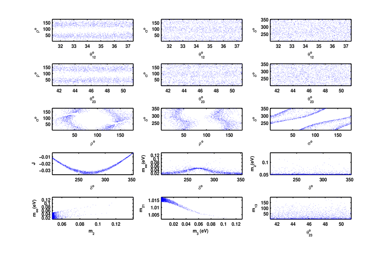
Figure 1: The correlation plots for traceless texture in case I (vanishing non-physical phases), in the inverted ordering hierarchy. The first and second row represent the correlations between the mixing angles ($\theta_{12}$,$\theta_{23}$) and the CP-violating phases. The third row introduces the correlations amdist the CP-violating phases, whereas the fourth one represents the correlations between the Dirac phase $\delta$ and each of $J$, $m_{ee}$ and $m_{2}$ parameters respectively. The last row shows the degree of mass hierarchy plus the ($m_{ee},m_{2}$) correlation.

As expected, no correlations involving $\theta_{y}$ exist since the coefficients $A_{i}$’s do not depend on this parameter. We note equally that no clear correlations involve $\theta_{x}$, whereas the correlations ($J,\delta$) follows a usual sine curve ($J\propto\sin\delta$) where the proportionality factor depends slightly on the mixing angles. We note also a small disallowed gap for $\rho$ around $\pi/2$

Regarding the mass parameters, we notice a correlation ($m_{ee},\delta$), which originates from those amidst ($\rho,\delta$) and ($\sigma,\delta$). The correlation ($m_{ee},m_{2}$) shows that $m_{ee}$ increases with increasing $m_{2}$, and that the hierarchy can be mildly strong reaching ($m_{13}\approx 10^{2}$), so $m_{3}$ can not vanish.

We reconstruct the neutrino mass matrix for a representative point, which is taken such that the mixing angles and the Dirac phase are chosen to be as near as possible from their best fit values from Table 1. For inverted ordering, the representative point is taken as follows.

$$(\theta_{12},\theta_{23},\theta_{13})= (35.74^{\circ},48.58^{\circ},8.55^{\circ}),$$ (21)

$$(\delta,\rho,\sigma)= (290.41^{\circ},28.58^{\circ},74.69^{\circ}),$$

$$(m_{1},m_{2},m_{3})= (0.0491\textrm{ eV},0.0499\textrm{ eV},0.0027\textrm{ eV}),$$

$$(m_{e},m_{ee},\Sigma)= (0.0489\textrm{ eV},0.0352\textrm{ eV},0.1017\textrm{ eV}),$$

and the corresponding neutrino mass matrix (in eV) is

$$M_{\nu}=\left(\begin{array}[]{ccc}0.0029+0.0351i&-0.0029-0.0259i&0.0033+0.0214i\\ \vskip 6.0pt plus 2.0pt minus 2.0pt\cr-0.0029-0.0259i&-0.0003-0.0103i&0.0041+0.0176i\\ \vskip 6.0pt plus 2.0pt minus 2.0pt\cr 0.0033+0.0214i&0.0041+0.0176i&-0.0026-0.0248i\end{array}\right).$$ (22)

4.1.2 Normal Hierarchy

Fig. (2) shows the correlations corresponding to normal hierarchy type.

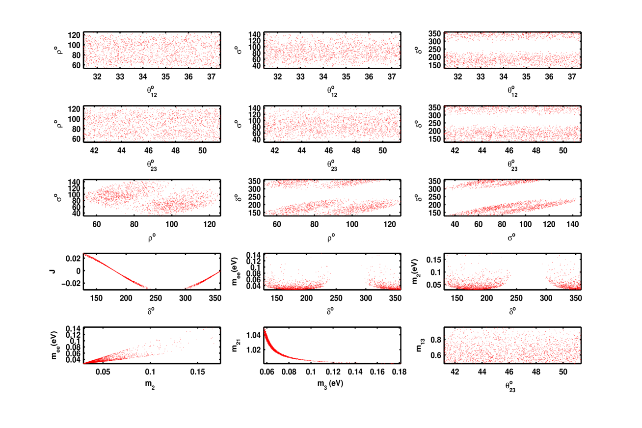
Figure 2: The correlation plots for traceless texture in case I (vanishing non-physical phases), in the normal ordering hierarchy. The first and second row represent the correlations between the mixing angles ($\theta_{12}$,$\theta_{23}$) and the CP-violating phases. The third row introduces the correlations amdist the CP-violating phases, whereas the fourth one represents the correlations between the Dirac phase $\delta$ and each of $J$, $m_{ee}$ and $m_{2}$ parameters respectively. The last row shows the degree of mass hierarchy plus the ($m_{ee},m_{2}$) correlation.

Again, no correlations involving $\theta_{y}$ as the coefficients $A_{i}$’s are $\theta_{y}$-independent. Also, no clear correlations involving $\theta_{x}$, whereas the correlations ($J,\delta$) is always sinusoidal in shape. There are disallowed gaps for ($\rho,\sigma$ and $\delta$).

Regarding the mass parameters, the correlation ($m_{ee},\delta$) results from those between ($\rho,\delta$) and ($\sigma,\delta$). The correlation ($m_{ee},m_{2}$) shows that $m_{ee}$ is increasing with respect to $m_{2}$, and that the hierarchy is weak characterized by ($m_{1}\approx m_{2}\approx m_{3}$), so $m_{1}$ can not vanish.

We reconstruct the neutrino mass matrix for a representative point, which is taken such that the mixing angles and the Dirac phase are chosen to be as near as possible from their best fit values from Table 1. For inverted ordering, the representative point is taken as follows.

$$(\theta_{12},\theta_{23},\theta_{13})= (35.81^{\circ},49.33^{\circ},8.56^{\circ}),$$ (23)

$$(\delta,\rho,\sigma)= (192.02^{\circ},98.22^{\circ},93.97^{\circ}),$$

$$(m_{1},m_{2},m_{3})= (0.0293\textrm{ eV},0.0305\textrm{ eV},0.0581\textrm{ eV}),$$

$$(m_{e},m_{ee},\Sigma)= (0.0306\textrm{ eV},0.0277\textrm{ eV},0.1179\textrm{ eV}),$$

and the corresponding neutrino mass matrix (in eV) is

$$M_{\nu}=\left(\begin{array}[]{ccc}-0.0269-0.0068i&0.0101-0.0006i&0.0079+0.0022i\\ \vskip 6.0pt plus 2.0pt minus 2.0pt\cr 0.0101-0.0006i&0.0198+0.0032i&0.0422-0.0036i\\ \vskip 6.0pt plus 2.0pt minus 2.0pt\cr 0.0079+0.0022i&0.0422-0.0036i&0.0071+0.0036i\end{array}\right).$$ (24)

4.2 Vanishing CP Phases

We note from table (2) that including the non-physical phases $\phi$ brings up a dependence on ($\theta_{x},\theta_{y}$) to the $A_{i}$’s coefficients.

Also, the numerical computations reveal a strong correlation between the non-physical phases, say ($\phi_{1},\phi_{2}$). This comes because we have:

$${M_{\nu}}_{ab}(\phi\neq 0)={M_{\nu}}_{ab}(\phi=0)e^{i(\phi_{a}+\phi_{b})} \Rightarrow {M_{\nu}}_{kk}(\phi\neq 0)=e^{2i\phi_{k}}{M_{\nu}}_{kk}(\phi=0)$$ (25)

and so the phases play an important role in meeting the traceless texture condition ($M_{\nu 11}+M_{\nu 22}+M_{\nu 33}=0$), since, as mentioned earlier, this condition can not be met with no phases at all. factoring out $e^{2i\phi_{3}}$, we drew the correlation ($\phi_{1}-\phi_{3},\phi_{2}-\phi_{3}$).

We noted that although $m_{1}$ ($m_{3}$) in the normal (inverted) hierarchy type can reach tiny values of order of ${\cal O}(10^{-7})\left({\cal O}(10^{-5})\right)$, however the singular texture with these masses equaling exactly zero was not achieved and singular textures are not accommodated.

4.2.1 Inverted Hierarchy

Fig. (3) shows the correlations corresponding to inverted hierarchy type.

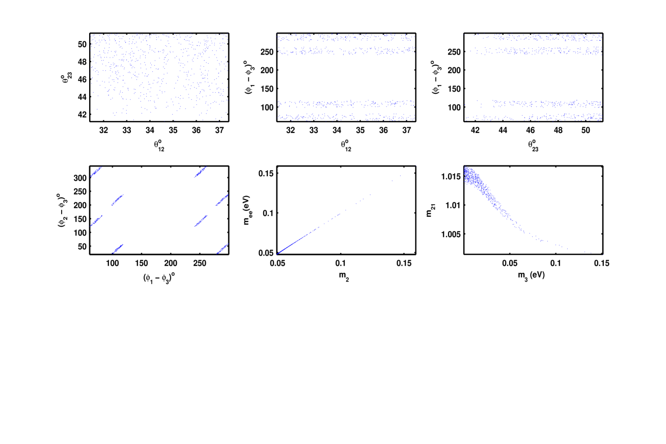
Figure 3: The correlation plots for traceless texture in case II (vanishing CP phases), in the inverted ordering hierarchy.

We note that the mixing angles $\theta$ and the non-physical phases $\phi$ cover all their allowed ranges without gaps. However, the differences ($\phi_{1}-\phi_{3}$) and ($\phi_{2}-\phi_{3}$) do have disallowed gaps.

We reconstruct the neutrino mass matrix for a representative point, which is taken such that the mixing angles are near their best fit values from Table 1. For inverted ordering, the representative point is taken as follows.

$$(\theta_{12},\theta_{23},\theta_{13})= (34.37^{\circ},49.10^{\circ},8.52^{\circ}),$$ (26)

$$(\phi_{1},\phi_{2},\phi_{3})= (59.06^{\circ},351.81^{\circ},130.23^{\circ}),$$

$$(m_{1},m_{2},m_{3})= (0.0515\textrm{ eV},0.0523\textrm{ eV},0.0151\textrm{ eV}),$$

$$(m_{e},m_{ee},\Sigma)= (0.0512\textrm{ eV},0.0510\textrm{ eV},0.1189\textrm{ eV}),$$

and the corresponding neutrino mass matrix (in eV) is

$$M_{\nu}=\left(\begin{array}[]{ccc}-0.0240+0.0449i&-0.0024-0.0030i&0.0037+0.0006i\\ \vskip 6.0pt plus 2.0pt minus 2.0pt\cr-0.0024-0.0030i&0.0301-0.0088i&0.0095-0.0151i\\ \vskip 6.0pt plus 2.0pt minus 2.0pt\cr 0.0037+0.0006i&0.0095-0.0151i&-0.0061-0.0361i\end{array}\right).$$ (27)

4.2.2 Normal Hierarchy

Fig. (4) shows the correlations corresponding to normal hierarchy type.

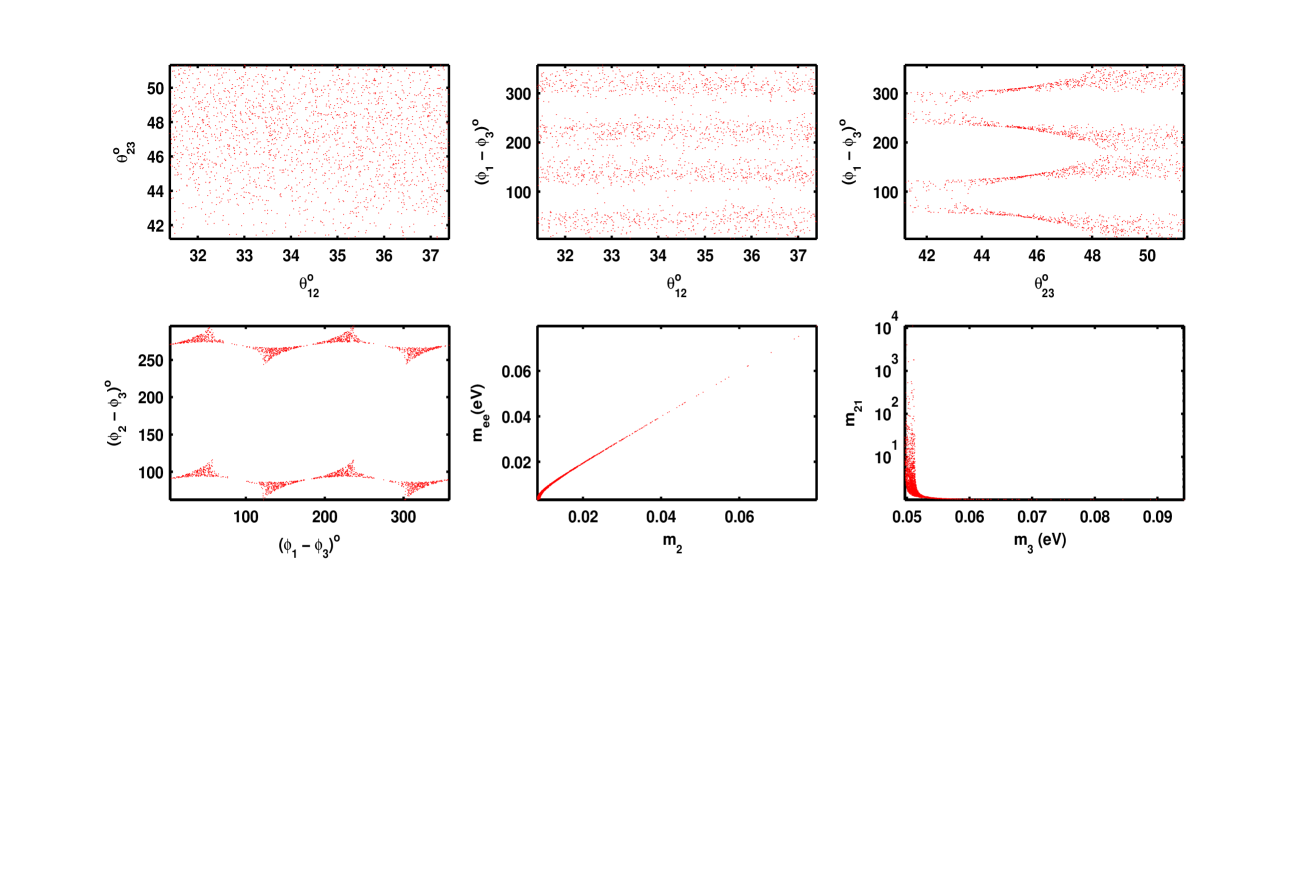
Figure 4: The correlation plots for traceless texture in case II (vanishing CP phases), in the normal ordering hierarchy.

We note again that the mixing angles $\theta$ and the non-physical phases $\phi$ cover all their allowed ranges without gaps, and that the differences ($\phi_{1}-\phi_{3}$) and ($\phi_{2}-\phi_{3}$) do have disallowed gaps.

We reconstruct the neutrino mass matrix for a representative point, which is taken such that the mixing angles are near from their best fit values from Table 1. For normal ordering, the representative point is taken as follows.

$$(\theta_{12},\theta_{23},\theta_{13})= (34.41^{\circ},49.16^{\circ},8.51^{\circ}),$$ (28)

$$(\phi_{1},\phi_{2},\phi_{3})= (248.68^{\circ},308.20^{\circ},24.07^{\circ}),$$

$$(m_{1},m_{2},m_{3})= (0.0164\textrm{ eV},0.0187\textrm{ eV},0.0538\textrm{ eV}),$$

$$(m_{e},m_{ee},\Sigma)= (0.0187\textrm{ eV},0.0179\textrm{ eV},0.0889\textrm{ eV}),$$

and the corresponding neutrino mass matrix (in eV) is

$$M_{\nu}=\left(\begin{array}[]{ccc}-0.0132+0.0121i&-0.0045-0.0014i&0.0001-0.0027i\\ \vskip 6.0pt plus 2.0pt minus 2.0pt\cr-0.0045-0.0014i&-0.0089-0.0368i&0.0154-0.0081i\\ \vskip 6.0pt plus 2.0pt minus 2.0pt\cr 0.0001-0.0027i&0.0154-0.0081i&0.0221+0.0247i\end{array}\right).$$ (29)

4.3 General case

In either hierarchy type, the mixing and phase (CP and non-physical) span their full ranges, with no corresponding gaps. Numerical computations reveal a weak correlations ($\phi_{1}-\phi_{3},\phi_{2}-\phi_{3}$), and that $m_{ee}$ is an increasing function of $m_{2}$. Like in (case II), the inclusion of the non-physical phases dilute many correlations compared to (case I), and so again we present just the six correlations described in (case II).

4.3.1 Inverted Hierarchy

Fig. (5) shows the correlations corresponding to inverted hierarchy type.

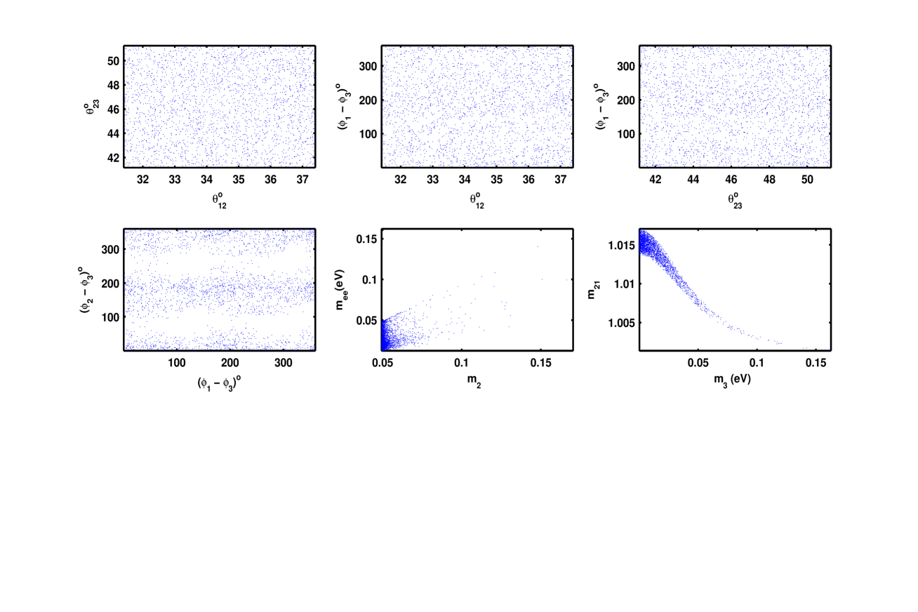
Figure 5: The correlation plots for traceless texture in case III (general), in the inverted ordering hierarchy.

Although $m_{3}$ can reach tiny values of order $m_{3}\succeq 2.73\times 10^{-6}$ eV, but numerically we checked that it can not reach zero exactly, and thus no singular patterns exist.

We reconstruct the neutrino mass matrix for a representative point, which is taken such that the mixing angles and Dirac phase are as close as possible to their best fit values from Table 1. For inverted ordering, the representative point is taken as follows.

$$(\theta_{12},\theta_{23},\theta_{13})= (34.82^{\circ},49.36^{\circ},8.51^{\circ}),$$ (30)

$$(\delta,\rho,\sigma)= (284.60^{\circ},52.50^{\circ},164.81^{\circ}),$$

$$(\phi_{1},\phi_{2},\phi_{3})= (39.25^{\circ},334.27^{\circ},326.31^{\circ}),$$

$$(m_{1},m_{2},m_{3})= (0.0900\textrm{ eV},0.0904\textrm{ eV},0.0750\textrm{ eV}),$$

$$(m_{e},m_{ee},\Sigma)= (0.0898\textrm{ eV},0.0442\textrm{ eV},0.2555\textrm{ eV}),$$

and the corresponding neutrino mass matrix (in eV) is

$$M_{\nu}=\left(\begin{array}[]{ccc}-0.0397+0.0195i&0.0488+0.0268i&-0.0451-0.0314i\\ \vskip 6.0pt plus 2.0pt minus 2.0pt\cr 0.0488+0.0268i&0.0147-0.0083i&0.0196-0.0544i\\ \vskip 6.0pt plus 2.0pt minus 2.0pt\cr-0.0451-0.0314i&0.0196-0.0544i&0.0249-0.0112i\end{array}\right).$$ (31)

4.3.2 Normal Hierarchy

Fig. (6) shows the correlations corresponding to inverted hierarchy type.

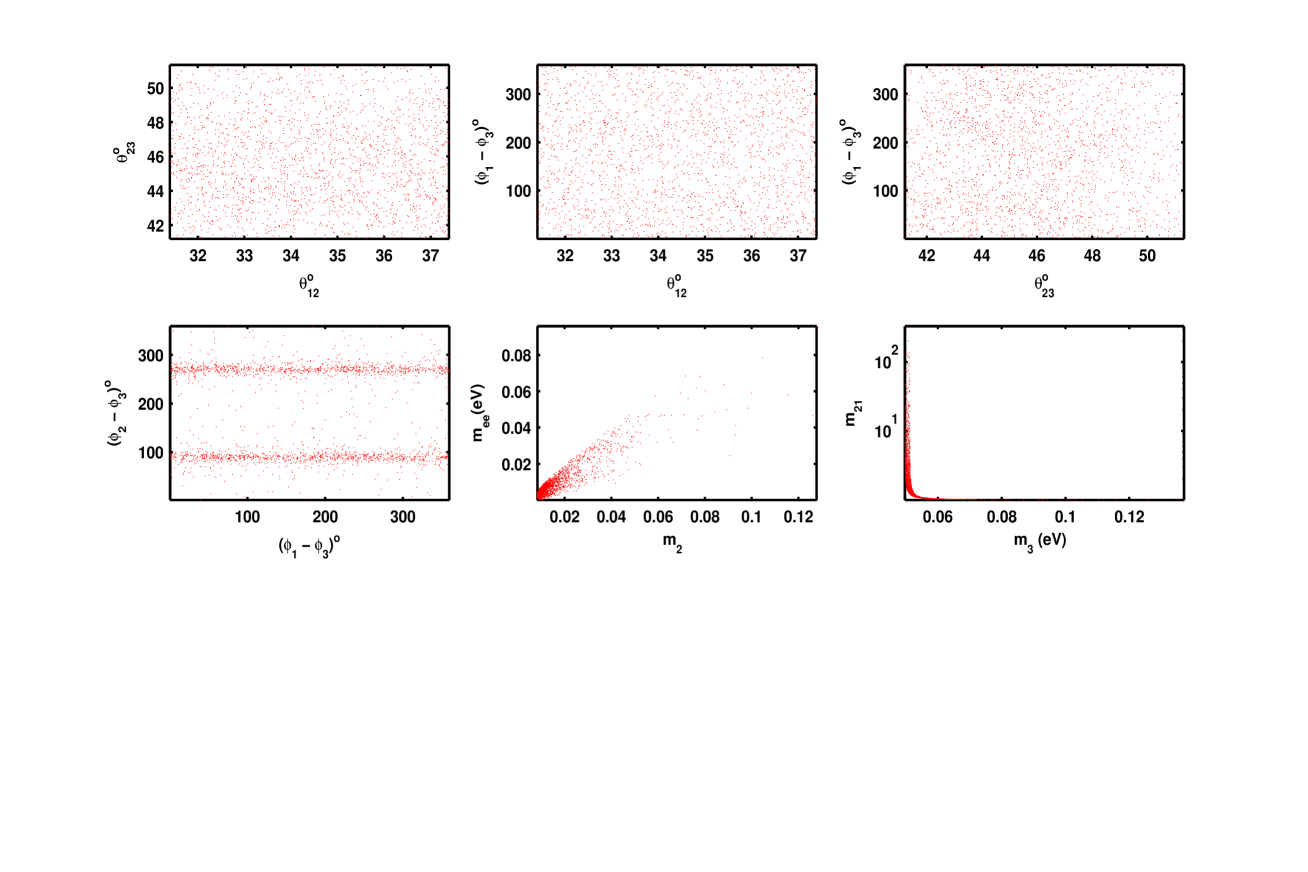
Figure 6: The correlation plots for traceless texture in case III (general), in the normal ordering hierarchy.

Although $m_{1}$ can reach tiny values of order $m_{1}\succeq 2.56\times 10^{-5}$ eV, but numerically we checked that it can not reach zero exactly, and thus no singular patterns exist.

We reconstruct the neutrino mass matrix for a representative point, which is taken such that the mixing angles and Dirac phase are as close as possible to their best fit values from Table 1. For normal ordering, the representative point is taken as follows.

$$(\theta_{12},\theta_{23},\theta_{13})= (34.33^{\circ},49.42^{\circ},8.55^{\circ}),$$ (32)

$$(\delta,\rho,\sigma)= (284.74^{\circ},170.22^{\circ},95.82^{\circ}),$$

$$(\phi_{1},\phi_{2},\phi_{3})= (32.16^{\circ},119.59^{\circ},45.10^{\circ}),$$

$$(m_{1},m_{2},m_{3})= (0.0314\textrm{ eV},0.0327\textrm{ eV},0.0592\textrm{ eV}),$$

$$(m_{e},m_{ee},\Sigma)= (0.0327\textrm{ eV},0.0143\textrm{ eV},0.1233\textrm{ eV}),$$

and the corresponding neutrino mass matrix (in eV) is

$$M_{\nu}=\left(\begin{array}[]{ccc}0.0130+0.006i&-0.0019+0.0199i&-0.0213+0.0029i\\ \vskip 6.0pt plus 2.0pt minus 2.0pt\cr-0.0019+0.0199i&-0.0088-0.0341i&-0.0240+0.0146i\\ \vskip 6.0pt plus 2.0pt minus 2.0pt\cr-0.0213+0.0029i&-0.0240+0.0146i&-0.0041+0.0280i\end{array}\right).$$ (33)

5 Theoretical realization

We present now one realization of the traceless texture based on $A_{5}$ non-abelian flavor symmetry within seesaw type II scenario. Although the matter content is extended beyond SM, to include new scalars, however we shall not discuss the question of the scalar potential and finding its general form under the imposed symmetry giving the required vacuum expectation values (VEVs). Actually, with new scalars, rich phenomenology at colliders may arise, and requesting only one SM-like Higgs at low scale is not a trivial task, and requires generally fine tuning.

5.1 $A_{5}$ group theory

The alternating group $A_{5}$ consists of even permutation between five elements. It is finite containing ($n_{G}=60$) elements which can be classified into five conjugation classes. Thus there are five independent unitary irreducible representations (irreps), which we call ($\bf 1,3,3^{\prime},4,5$). We state now the multiplication rules for these irreps (Eq. 34), and put also the SALC (symmetry adapted linear combinations) which would serve us in constructing the model when multiplying two triplets (Eq. 50), with the singlet combination when multiplying two quantuplets (Eq. 51).

$${\bf 3}\otimes{\bf 3}={\bf 1}\oplus{\bf 3}\oplus{\bf 5} {\bf 3^{\prime}}\otimes{\bf 3^{\prime}}={\bf 1}\oplus{\bf 3^{\prime}}\oplus{\bf 5},$$ , (34)

$${\bf 3}\otimes{\bf 3^{\prime}}={\bf 4}\oplus{\bf 5} {\bf 4}\otimes{\bf 5}={\bf 3}\oplus{\bf 3^{\prime}}\oplus{\bf 4}\oplus{\bf 5}\oplus{\bf 5},$$ ,

$${\bf 3}\otimes{\bf 4}={\bf 3^{\prime}}\oplus{\bf 4}\oplus{\bf 5} {\bf 3^{\prime}}\otimes{\bf 4}={\bf 3}\oplus{\bf 4}\oplus{\bf 5}$$ ,

$${\bf 3}\otimes{\bf 5}={\bf 3}\oplus{\bf 3^{\prime}}\oplus{\bf 4}\oplus{\bf 5} {\bf 3^{\prime}}\otimes{\bf 5}={\bf 3}\oplus{\bf 3^{\prime}}\oplus{\bf 4}\oplus{\bf 5}$$ ,

$${\bf 4}\otimes{\bf 4}={\bf 1}\oplus{\bf 3}\oplus{\bf 3^{\prime}}\oplus{\bf 4}\oplus{\bf 5} {\bf 5}\otimes{\bf 5}={\bf 1}\oplus{\bf 3}\oplus{\bf 3^{\prime}}\oplus{\bf 4}\oplus{\bf 4}\oplus{\bf 5}\oplus{\bf 5},$$ ,

$$\left(\begin{array}[]{l}a_{1}\\ a_{2}\\ a_{3}\end{array}\right)_{\bf 3}\otimes\left(\begin{array}[]{l}b_{1}\\ b_{2}\\ b_{3}\end{array}\right)_{\bf 3} = \left(a_{1}b_{1}+a_{2}b_{2}+a_{3}b_{3}\right)_{\bf 1}\oplus\left(\begin{array}[]{c}a_{3}b_{2}-a_{2}b_{3}\\ a_{1}b_{3}-a_{3}b_{1}\\ a_{2}b_{1}-a_{1}b_{2}\end{array}\right)_{\bf 3}$$ (50)

$$\oplus\left(\begin{array}[]{c}a_{2}b_{2}-a_{1}b_{1}\\ a_{2}b_{1}+a_{1}b_{2}\\ a_{3}b_{2}+a_{2}b_{3}\\ a_{1}b_{3}+a_{3}b_{1}\\ -\frac{1}{\sqrt{3}}\left(a_{1}b_{1}+a_{2}b_{2}-2a_{3}b_{3}\right)\end{array}\right)_{\bf 5},$$

$$\left(a_{1},a_{2},a_{3},a_{4},a_{5}\right)^{T}_{\bf 5}\otimes\left(b_{1},b_{2},b_{3},b_{4},b_{5}\right)^{T}_{\bf 5} \supset \left(a_{1}b_{1}+a_{2}b_{2}+a_{3}b_{3}+a_{4}b_{4}+a_{5}b_{5}\right)_{\bf 1}$$ (51)

5.1.1 Type-II Seesaw Matter Content:

For the type-II seesaw scenario leading to a traceless texture of the neutrino mass matrix, we take the matter content shown in Table (4)

Table 4: matter content and symmetry transformations, leading to traceless texture. $\Delta_{j}=\left(\begin{array}[]{cc}\Delta^{+}_{j}&\Delta^{++}_{j}\\ \Delta^{0}_{j}&-\Delta^{+}_{j}\end{array}\right)$, $j=1,\ldots,5$ with $i=1,2,3$ is a family index.

Fields	$D_{L_{i}}$	$\Delta_{j}$	$\ell_{R_{i}}$	$\phi_{I}$	$\phi_{{III}_{i}}$	$\phi_{V_{j}}$
$SU(2)_{L}$	2	3	1	2	2	2
$A_{5}$	${\bf 3}$	${\bf 5}$	${\bf 3}$	${\bf 1}$	${\bf 3}$	${\bf 5}$

The Lorentz-, gauge- and $A_{5}$-invariant terms relevant for the neutrino mass matrix are

$${\cal L}\ni\left(D_{L}^{T}D_{L}\Delta\right)_{\bf 1} = Y\left[\left(D^{T}_{L\mu}C^{-1}i\tau_{2}D_{L\mu}-D^{T}_{Le}C^{-1}i\tau_{2}D_{Le}\right)\Delta_{1}\right.$$ (52)

$$+\left(D^{T}_{L\mu}C^{-1}i\tau_{2}D_{Le}+D^{T}_{Le}C^{-1}i\tau_{2}D_{L\mu}\right)\Delta_{2}$$

$$+\left(D^{T}_{L\tau}C^{-1}i\tau_{2}D_{L\mu}+D^{T}_{L\mu}C^{-1}i\tau_{2}D_{L\tau}\right)\Delta_{3}$$

$$+\left(D^{T}_{Le}C^{-1}i\tau_{2}D_{L\tau}+D^{T}_{L\tau}C^{-1}i\tau_{2}D_{Le}\right)\Delta_{4}$$

$$-\frac{1}{\sqrt{3}}\left(D^{T}_{Le}C^{-1}i\tau_{2}D_{Le}+D^{T}_{L\mu}C^{-1}i\tau_{2}D_{L\mu}-2D^{T}_{L\tau}C^{-1}i\tau_{2}D_{L\tau}\right)\Delta_{5}\left.\right]$$

This $Y$-term picks up the quintuplet combination from the product of the two triplets ($D^{T}_{L_{i}}$ and $D_{L_{i}}$) (Eq. 50), before multiplying it with the Higgs flavor quintuplet $\Delta_{j}$ in order to get a singlet according to Eq. (51). We get, upon acquiring small VEVs for the neutral components of $\Delta_{j}^{o},j=1,\ldots,5$, denoted by $v_{j}$ and set by the Lagrangian free parameters, the following neutrino mass matrix

$$M_{\nu} = Y\left(\begin{array}[]{ccc}-\frac{1}{\sqrt{3}}v_{5}-v_{1}&v_{2}&v_{4}\\ v_{2}&-\frac{1}{\sqrt{3}}v_{5}+v_{1}&v_{3}\\ v_{4}&v_{3}&\frac{2}{\sqrt{3}}v_{5}\end{array}\right)$$ (56)

We see that this texture meets the traceless condition $\left[\mbox{Tr}(M_{\nu})=0\right]$.

5.1.2 Charged lepton sector:

We can build a generic mass matrix and impose suitable hierarchy conditions in order to diagonlize $M_{\ell}$ by rotating infinitesimally the left-handed charged lepton fields. This means that, up to approximations of the order of the charged lepton mass-ratios hierarchies, we are in the ‘flavor’ basis, and the previous phenomenological study is valid. These corrections due to rotating the fields are not larger than other, hitherto discarded, corrections coming, say, from radiative renormalization group running from the seesaw high scale to the observed data low scale.

The Lorentz-, gauge- and $A_{5}$-invariant terms relevant for the charged lepton mass are

$${\cal L}\ni\left(\Sigma_{a=I,III,V}\overline{D_{L}}\ell_{R}\;\phi_{a}\right)_{\bf 1} = Y_{I}\left(\overline{D}_{Le}e_{R}+\overline{D}_{L\mu}\mu_{R}+\overline{D}_{L\tau}\tau_{R}\right)\phi_{I}$$ (57)

$$+Y_{III}\left[\right.\left(\overline{D}_{L\tau}\mu_{R}-\overline{D}_{L\mu}\tau_{R}\right)\phi_{III_{1}}+\left(\overline{D}_{Le}\tau_{R}-\overline{D}_{L\tau}e_{R}\right)\phi_{III_{2}}$$

$$+\left(\overline{D}_{L\mu}e_{R}-\overline{D}_{Le}\mu_{R}\right)\phi_{III_{3}}\left.\right]$$

$$+Y_{V}\left[\left(\overline{D}_{L\mu}\mu_{R}-\overline{D}_{Le}e_{R}\right)\phi_{V_{1}}\right.+\left(\overline{D}_{L\mu}e_{R}+\overline{D}_{Le}\mu_{R}\right)\phi_{V_{2}}$$

$$+\left(\overline{D}_{L\tau}\mu_{R}+\overline{D}_{L\mu}\tau_{R}\right)\phi_{V_{3}}+\left(\overline{D}_{Le}\tau_{R}+\overline{D}_{L\tau}e_{R}\right)\phi_{V_{4}}$$

$$-\frac{1}{\sqrt{3}}\left(\overline{D}_{Le}e_{R}+\overline{D}_{L\mu}\mu_{R}-2\overline{D}_{L\tau}\tau_{R}\right)\phi_{V_{5}}\left.\right]$$

which leads, when $\phi_{a},a\in\{I,III,V\}$ acquires a VEV, to a charged lepton mass:

$$M_{\ell} = Y_{I}\langle\phi_{I}\rangle_{0}\left(\begin{array}[]{ccc}1&0&0\\ 0&1&0\\ 0&0&1\end{array}\right)+Y_{III}\left(\begin{array}[]{ccc}0&-\langle\phi_{III_{3}}\rangle_{0}&\langle\phi_{III_{2}}\rangle_{0}\\ \langle\phi_{III_{3}}\rangle_{0}&0&-\langle\phi_{III_{1}}\rangle_{0}\\ -\langle\phi_{III_{2}}\rangle_{0}&\langle\phi_{III_{1}}\rangle_{0}&0\end{array}\right)$$ (68)

$$+Y_{V}\left(\begin{array}[]{ccc}-\frac{1}{\sqrt{3}}\langle\phi_{V_{5}}\rangle_{0}-\langle\phi_{V_{1}}\rangle_{0}&\langle\phi_{V_{2}}\rangle_{0}&\langle\phi_{V_{4}}\rangle_{0}\\ \langle\phi_{V_{2}}\rangle_{0}&-\frac{1}{\sqrt{3}}\langle\phi_{V_{5}}\rangle_{0}+\langle\phi_{V_{1}}\rangle_{0}&\langle\phi_{V_{3}}\rangle_{0}\\ \langle\phi_{V_{4}}\rangle_{0}&\langle\phi_{V_{3}}\rangle_{0}&\frac{2}{\sqrt{3}}\langle\phi_{V_{5}}\rangle_{0}\end{array}\right).$$

Two common ways to get a generic $M_{\ell}$.

• We assume a VEV hierarchy such that the $(\langle\phi_{I}\rangle_{0},\langle\phi_{V_{1}}\rangle_{0},\langle\phi_{V_{5}}\rangle_{0})$ are dominant , and we get approximately a diagonal matrix

  $$M_{\ell} \approx \mbox{diag}\left(M_{\ell 11},M_{\ell 22},M_{\ell 33}\right):$$ (69)

  $$M_{\ell 11} = Y_{I}\langle\phi_{I}\rangle_{0}-\frac{1}{\sqrt{3}}Y_{V}\langle\phi_{V_{5}}\rangle_{0}-Y_{V}\langle\phi_{V_{1}}\rangle_{0},$$

  $$M_{\ell 22} = Y_{I}\langle\phi_{I}\rangle_{0}-\frac{1}{\sqrt{3}}Y_{V}\langle\phi_{V_{5}}\rangle_{0}+Y_{V}\langle\phi_{V_{1}}\rangle_{0},$$

  $$M_{\ell 33} = Y_{I}\langle\phi_{I}\rangle_{0}+\frac{2}{\sqrt{3}}Y_{V}\langle\phi_{V_{5}}\rangle_{0}.$$

  With the free two Yukawa couplings and three VEVs, one can accommodate the observed charged lepton masses. Thus, as long as the neglected VEVs are sufficiently small, the rotation into the ‘flavor’ basis is done via infintesimal rotations.

• Looking at Eq. (68), we see that we have 9 free VEVs and 3 free perturbative coupling constants, appearing in 9 linear independent combinations, a priori enough to construct the generic $3\times 3$ complex matrix. Thus, $M_{\ell}$ can be casted in the form

  $$M_{\ell}=\left(\begin{array}[]{c}{\bf a}^{T}\\ {\bf b}^{T}\\ {\bf c}^{T}\end{array}\right) \Rightarrow M_{\ell}M_{\ell}^{\dagger}=\left(\begin{array}[]{ccc}{\bf a.a}&{\bf a.b}&{\bf a.c}\\ {\bf b.a}&{\bf b.b}&{\bf b.c}\\ {\bf c.a}&{\bf c.b}&{\bf c.c}\end{array}\right)$$ (76)

  where ${\bf a},{\bf b}$ and ${\bf c}$ are three linearly independent vectors, so taking only the following natural assumption on the norms of the vectors

  $$\parallel{\bf a}\parallel/\parallel{\bf c}\parallel=m_{e}/m_{\tau}\sim 3\times 10^{-4} \parallel{\bf b}\parallel/\parallel{\bf c}\parallel=m_{\mu}/m_{\tau}\sim 6\times 10^{-2}$$ , (77)

  one can diagonalize $M_{\ell}M_{\ell}^{\dagger}$ by an infinitesimal rotation as was done in [3], which proves that we are to a good approximation in the flavor basis.

6 Summary and Conclusion

In this study, we have reviewed the traceless texture for neutrino mass matrix, and have carried out a systematic study highlighting the role played by all phases. Switching off the non-physical phases, leads to acceptable traceless texture accommodating both types of hierarchy. Previous studies assuming vanishing non-physical phases should be looked at as being corresponding to a new texture, otherwise one could not a priori limit the study to the vanishing non-physical phases slice. Restoring the non-physical phases while turning off the CP phases allows also for both hierarchy types.

When including the non-physical phases, we find that many correlations get “diluted” (voire “disappeared”), since, with these non-physical phases not necessarily zero, one can find many more points in the parameter space meeting the experimental constraints and the mathematical traceless condition. One should comment that upon introducing non-physical phases then the different parameterizations, related to each other by certain relations [17], give the same correlations, when adjusted to correspond to the same definitions, and same phenomenology, as was explicitly checked by us.

Finally, we presented a theoretical realization of these textures via a type-II seesaw scenario and assuming a non-abelian group $A_{5}$. However, we have not discussed the question of the scalar potential and finding its general form under the imposed symmetry. Nor did we deal with the radiative corrections effect on the phenomenology and whether or not it can spoil the form of the texture while running from the seesaw “ultraviolet” scale, where the traceless condition is imposed, to the low scale where phenomenology was analyzed.

References

- [1] P. F. Harrison, D. H. Perkins and W. G. Scott, Phys. Lett. B 530, (2002) 167; P. F. Harrison and W. G. Scott, Phys. Lett. B 535, (2002) 163-169; Z. z. Xing, Phys. Lett. B 533, (2002) 85-93; E. I. Lashin, M. Abbas, N. Chamoun, and S. Nasri, Phys. Rev. D 86, 033013 (2012).
- [2] A. Merle and W. Rodejohann, Phys. Rev. D 73 (2006) 073012.
- [3] E. I. Lashin and N. Chamoun, Phys. Rev. D 85 (2012) 113011
- [4] Paul H. Frampton, Sheldon L. Glashow and Danny Marfatia, Phys. Lett. B 536 (2002) 79
- [5] Zhi-Zhong Xing, Pjys. Lett B 530 (2002) 159
- [6] E. I. Lashin and N. Chamoun, Phys. Rev. D 78 (2008) 073002
- [7] H. A. Alhendi, E. I. Lashin and A. A. Mudlej, Phys. Rev. D 77 (2008) 013009
- [8] A. Ismael, E. I. Lashin and N. Chamoun, Phys. Rev. D 107, 035017
- [9] S. Dev, Radha Raman Gautam and Lal Singh, Phys. Rev. D 87 (2013) 073011
- [10] S. Kaneko, H. Sawanaka and M. Tanimoto, JHEP 0508, (2005) 073; S. Dev, S. Verma and S. Gupta, Phys. Lett. B 687, (2010) 53-56; W. Wang, Eur. Phys. J. C 73, (2013) 2551; S. Dev, R. R. Gautam and L. Singh, Phys. Rev. D 88, (2013) 033008; S. Dev and D. Raj, Nucl. Phys. B 957, (2020) 115081
- [11] D. Black, A. Fariborz, S. Nasri and J. Schechter, Phys. Rev. D 62 (2000) 073015,
- [12] S. Nasri, J. Schechter and S. Moussa, Phys. Rev. D 70 (2004) 053005,
- [13] S. Masood, S. Nasri and J. Schechter, Phys. Rev. D 71 (2005) 093005,
- [14] X.-G. He and A. Zee, Phys. Rev. D 68 (2003) 037302,
- [15] W. Rodejohann, Phys. Lett. B 579 (2004) 127,
- [16] A. Ismael, E.I. Lashin, M. AlKhateeb and N. Chamoun, Nucl. Phys. B. 971 (2021) 115541
- [17] N. Chamoun and E.I. Lashin, arXiv: 2308.10985 (2023)
- [18] M. Singh, Adv. High Energy Physics (2018) 2863184,
- [19] S. Dey and M. Patgiri, Phys. Rev. D 107 (2023) 035012
- [20] H. Fritzsch and Z.-z. Xing, Phys. Lett. B 517 (2001) 363.
- [21] Z.-z. Xing, J. Phys. G, Nucl. Part. Phys. 28 (2002) 7.
- [22] P. F. de Salas, D. V. Forero, S. Gariazzo, P. Martinez-Mirave, O. Mena, C. A. Ternes, M. Tortola and J. W. F. Valle, JHEP 02 (2021) 071
- [23] KATRIN collaboration, Phys. Rev. Lett. 123 (2019) 221802
- [24] GERDA collaboration, Science 365 (2019) 1445
- [25] Planck Collaboration, Astronomy Astrophysics 641 (2020) A6
- [26] E. Di Valentino, S. Gariazzo and O. Mena, Phys. Rev. D, 104 (2021) 083504,
- [27] Z. Chacko, A. Dev, P. Du, V. Poulinb and Y. Tsaia, JHEP, 04 (2020) 020.