A Theoretical Explanation of Activation Sparsity through Flat Minima and Adversarial Robustness
Abstract
A recent empirical observation (Li et al., 2022b) of activation sparsity in MLP blocks offers an opportunity to drastically reduce computation costs for free. Although having attributed it to training dynamics, existing theoretical explanations of activation sparsity are restricted to shallow networks, small training steps and special training, despite its emergence in deep models standardly trained for a large number of steps. To fill these gaps, we propose the notion of gradient sparsity as one source of activation sparsity and a theoretical explanation based on it that sees sparsity as a necessary step to adversarial robustness w.r.t. hidden features and parameters, which is approximately the flatness of minima for well-learned models. The theory applies to standardly trained LayerNorm-ed MLPs, and further to Transformers or other architectures trained with weight noises. Eliminating other sources of flatness except for sparsity, we discover the phenomenon that the ratio between the largest and smallest non-zero singular values of weight matrices is small. When discussing the emergence of this spectral concentration, we use random matrix theory (RMT) as a powerful tool to analyze stochastic gradient noises. Experiments for validation are conducted to verify our gradient-sparsity-based explanation. We propose two plug-and-play modules for both training and finetuning for sparsity. Experiments on ImageNet-1K and C4 demonstrate their sparsity improvements, indicating further potential cost reduction in both training and inference.
Keywords: sparsity, flat minima, training dynamics, random matrix theory, deep learning
1 Introduction
Despite the success of overparameterized deep neural networks, how they learn, work and generalize well is not fully understood. Although more than half of parameters and computation are devoted to them (Dai et al., 2022), even in Transformers, MLP blocks have remained black box for years, blocking interpretation, manipulation and pruning in them. Recently, some works (Geva et al., 2021; Dai et al., 2022) have tried to dive into MLP blocks and reveal its relation with learned knowledge by rewriting MLP blocks of Transformers into an attention mechanism where keys and values are provided by the first and second linear layers, and form a key-value memory that stores learned knowledge.
A more recent work (Li et al., 2022b) further discovers activation sparsity in MLP blocks, i.e., only a small portion of neurons are activated during inference, within MLP blocks of pure MLP, ResNet, T5, () ViT and other architectures on various tasks, without explicit regularization. This discovery not only brings research attention back to MLP blocks when it comes to understanding Transformers but also leads to potential aggressive but unstructured and dynamic neuron pruning during inference and thus large reduction in inference cost. Specifically, if pruning is ideally implemented to skip non-activated neurons, theoretically in T5 the inference costs happening in MLP blocks can be astonishingly reduced by about . There is also an increasing tendency of activation sparsity, measured in percentage of zero activations, when models become larger (Li et al., 2022b), hinting at potentially great cost reduction for large models. Activation sparsity in CNNs, although weaker (Li et al., 2022b; Kurtz et al., 2020), has been exploited to provide on-the-fly pruning or compression during inference (Kurtz et al., 2020).
However, the emergence of sparsity is not yet fully understood. Several works (Li et al., 2022b; Andriushchenko et al., 2023a, b; Bricken et al., 2023) have been proposed to explain the emergence of sparsity from training dynamics. Li et al. (2022b) explain activation sparsity of the last layer during the first step by computing gradients and exploiting properties of initialization methods. When sharpness-aware optimization is used, Andriushchenko et al. (2023a) find positive components in gradients that point towards norm reduction of activations. However, only a shallow 2-layer MLP is studied by Andriushchenko et al. (2023a). Andriushchenko et al. (2023b) consider second-order behaviors of SGD and proves sparsity on diagonal 2-layer MLPs, but for general networks it is only conjectured. Bricken et al. (2023) find that noises added to samples improve sparsity. However, the noises are manually imposed and are not included in standard augmentations. Although having achieved better understanding on sparsity and training dynamics and hinting at the roles of noises and flatness in activation sparsity, these works are still restricted to shallow networks, small steps, additional regularization or augmentations that cannot be found in ubiquitous training protocols. Nevertheless, they point out the role of flatness or noises in the emergence of sparsity.
Filling the gap between experiments and these theoretical results, we propose a new theoretical explanation that applies to deep networks, large training steps and standard training practices, by further emphasizing flatness and noises. In particular, we first rewrite the flatness bias of SGD into a tendency to improve implicit adversarial robustness w.r.t. hidden features and parameters. Gradient sparsity and effective gradient sparsity are proposed as causes of activation sparsity. To support this, we prove a theorem stating that these kinds of sparsity can be one of the sources of implicit adversarial robustness. Since flat minima bias puts constraints on all layers, basing our explanation on this inductive bias allows us to reason about deep layers. To eliminate other potential sources of implicit adversarial robustness, we exploit LayerNorm layers, refer to an already discovered inductive bias called parameter growth (Merrill et al., 2021) and empirically discover a new phenomenon of spectral concentration, i.e., the fraction between the largest and smallest non-zero singular values of the first weight matrices in MLP blocks is not very large. We prove the emergence of spectral concentration at initialization. We also theoretically discuss its re-emergence and maintenance during later training using random matrix theory (RMT) by extracting from stochastic gradients two large random matrices, indicating that training stochasticity’s contribution to sparsity is two-folded. Notably, thanks to RMT our formulation of stochastic gradient noises is very direct, without assuming Gaussian or distributions on them but uniform and independent sampling within a batch and bounds on anisotropy and gradient norms that can be estimated empirically. Following these theoretical insights, we propose two plug-and-play and orthogonal architectural modifications, which brings relatively approximately training sparsity improvements and at least on testing sparsity compared to existing naturally emergent sparsity of or non-zero activations. The structure of this work is as follows:
-
•
In Section 3, we introduce preliminaries and background information. But in Section 3.2, we propose gradient sparsity, distinguish it from activation sparsity and argue its importance over activation sparsity;
-
•
In Section 4.1, we build an intuitive framework of our explanation from flat minima and implicit adversarial robustness. Two almost plug-and-play architectural modifications, and , are proposed to further improve sparsity and ease formal analyses;
-
•
In Section 4.2, gradients of MLP blocks are computed, laying the basis for later formal analyses. Effective gradient sparsity is defined in this subsection, and its connection with training updates as well as gradient sparsity is discussed. Specifically, Lemma connects effective gradient sparsity measure in norms to activation sparsity directly measured in norms for networks, while the similar connection under is approximately discussed;
-
•
In Section 4.3, we prove Theorem that relates flat minima and implicit adversarial robustness to effective gradient sparsity and activation sparsity by proving relatively tight chained upperbounds among them, demonstrating that sparsity can be the source of implicit adversarial robustness imposed by flat minima;
-
•
In Section 4.4, we instantiate Theorem in several specific settings involving pure MLPs and Transformers. Among them, Theorem proves the tendency toward effective gradient sparsity on pure MLPs with LayerNorms. We argue that effective gradient sparsity is more stable and powerful during the entire training than direct activation sparsity. Theorem deals with Transformers and other architectures by assuming perturbation training like dropout or tokenwise synapse noises. Another under-testing module called is immediate after Theorem and is elaborated on in Appendix F. We discuss the effectiveness of zeroth biases in the rest of this subsection. Aside from effective gradient sparsity, implicit adversarial robustness and flatness can potentially be achieved by reducing norms of a matrix or misaligning gradients with that matrix in the term brought by our modification. To eliminate the first, the already discovered phenomenon of parameter growth is exploited. The latter is handled in later subsections.
-
•
Eliminating the latter, we discover another phenomenon in ViT and T5 that most non-zero eigenvalues of the matrix differ by at most 100 times for most of the time, leaving only two possibilities: adversarial robustness is achieved only by (effective) gradient sparsity, or back-propagated gradients are totally lost. In Section 4.5, we prove the emergence of this spectral concentration at initialization, exploiting modern initialization techniques. A drastic architectural modification, wide MLPs, is proposed to fill a gap of theories;
-
•
In Section 4.6 we discuss spectral concentration’s maintenance and re-emergence in latter stochastic training, applying random matrix theory by extracting two large random matrices from the updates to the weight matrices;
- •
-
•
In Section 6, we conduct experiments 1) to show that activation sparsity can be lost but gradient sparsity is stable, and 2) to verify our explanation;
-
•
In Section 7, we train modified ViT-Base/16 on ImageNet-1K as well as T5-Base on C4 from scratch to examine the effectiveness of our modifications in the sense of sparsity and further verify our explanation. We also finetune trained weights for sparsity after plugging the two modifications to demonstrate a cheaper way to become sparser;
-
•
In Section 8, assumptions made in Section 4.3 and Section 4.6 are examined empirically.
To summarize our contribution, we propose the notions of gradient sparsity, effective gradient sparsity and implicit adversarial robustness. We explain activation sparsity with flat minima and implicit adversarial robustness, and propose two architectural theoretically guided modifications to improve sparsity. The benefits of LayerNorm layers and the practice of excluding their parameters from weight decay are emphasized in theories and experiments. To our knowledge, we are the first to utilize random matrix theory to reason about inductive biases of stochastic training. As a result, the modeling of stochastic gradient noises (SGN) is very direct and avoids any debatable SGN modeling like Gaussian or models. Experiments show that our explanation is more applicable than other potential ones and our modification further improves activation sparsity by a large margin.
2 Related Works
In this section, we list works on the same topic as ours. Section 3 contains works on different topics that our explanation depends on, we omit their details for simplicity here.
In our point of view, the research of activation sparsity in MLP modules starts from the discovery of the relation between MLP and knowledge gained during training. Geva et al. (2021) first rewrite MLPs in Transformers into an unnormalized attention mechanism where queries are inputs to the MLP block while keys and values are provided by the first and second weight matrices instead of inputs. So MLP blocks are key-value memories. Dai et al. (2022) push forward by detecting how each key-value pair is related to each question exploiting activation magnitudes as well as their gradients, and providing a method to surgically manipulate answers for individual questions in Q&A tasks. These works reorient research attention back to MLPs, which are previously shadowed by self-attention.
Recently, comprehensive experiments conducted by Li et al. (2022b) demonstrate activation sparsity in MLPs is a prevailing phenomenon in various architectures and on various CV and NLP tasks. Li et al. (2022b) also eliminate alternative explanations and attribute activation sparsity solely to training dynamics. The authors explain the sparsity theoretically with initialization and by calculating gradients, but their explanation is restricted to the last layer and the first step because in later steps the independence between weights and samples required by the explanation is broken. They also discover that some activation functions, such as , hinder the sparsity (see Li et al., 2022b, Fig B.3(c)), but did not elaborate on it. Compared to their explanations, our explanation applies to all layers and large steps, and accounts for the activation functions’ critical role in activation sparsity.
Following empirical discoveries by Li et al. (2022b), Andriushchenko et al. (2023a) show that sharpness-aware (SA) optimization has a stronger bias toward activation sparsity. They explain theoretically by calculating gradients and finding that SA optimization imposes in gradients a component toward reducing norms of activations. However, their explanation is still conducted on shallow 2-layer pure MLPs and requires SA optimization, which is not included in standard training practice. Nevertheless, this explanation hints at the role of flatness in the emergence of activation sparsity. Inspired by them, we explain deep networks trained by standard SGD or other stochastic trainers by substituting flat minima for SA optimization.
A more recent work by Bricken et al. (2023) holds a point that sparsity is a resistance to noises. However, noises are manually imposed and not included in standard data augmentations. We substitute gradient noise from SGD or other stochastic optimizers for them. Andriushchenko et al. (2023b) prove sparsity on 2-layer diagonal MLPs and conjecture similar things to happen in more general networks. Both works hint at the relation between noises (Gaussian sample noises and stochastic gradient noises) and activation sparsity, also leading to the flatness bias of stochastic optimization.
Puigcerver et al. (2022) study the adversarial robustness of Mixture of Experts (MoE) models brought by architecture-imposed sparsity. They inspire us to relate sparsity with adversarial robustness, although we do it reversely. It is the major inspiration for our results.
To sum up, existing discoveries hint at the relation between activation sparsity and noises, flatness and activation functions but they are still restricted to shallow layers, small steps and special training. Inspired by them and filling their gaps, our explanation applies to deep networks and large training steps, and sticks to standard training procedures.
Although not devoting much to explaining the emergence of activation sparsity in CNNs, Kurtz et al. (2020) boost activation sparsity through Hoyer regularization(Hoyer, 2004) and a new activation function FATReLU that uses dynamic thresholds between activation and deactivation. They also design algorithms to exploit this sparsity, leading to speedup in CNN’s inference. Compared to their sparsity encouragement method that requires well-designed procedures to select thresholds, hyperparameters for our theoretically induced modifications can be easily selected. The discontinuity of FATReLU also bothers training from scratch(Kurtz et al., 2020), while we recommend applying our modifications from scratch to enjoy better sparsity and additionally smaller training costs. Regarding exploitation, we consider it out of the manuscript’s scope. Georgiadis (2019) encourages activation sparsity in CNN by explicit regularization. We intend to investigate the emergence of activation sparsity from implicit regularization as demonstrated by Li et al. (2022b), so we solely rely on implicit regularization boosted by modifications. Nevertheless, our methods are architecturally orthogonal and we believe applying both together can further boost activation sparsity.
There are other works that are not devoted to activation sparsity but are related. Ren et al. (2023) formulate, with Shapley value, and prove that there are sparse “symbols” as groups of patches that are the only major contributors to the output of any well-trained and masking-robust AIs. They provide a sparsity independent of training dynamics. Their theory focuses on symbols and sparsity in inputs, which is inherently different from ours.
In Primer (So et al., ), several architectural changes given by architecture searching include a new activation function Squared-ReLU. In this work, we induce a similar squared activation but with the non-zero part shifted left and use it to guide the search for flat minima and gradient/activation sparsity. So et al. demonstrate impressive improvements of Squared-ReLU in both ablation and addition experiments, and our work provides a potential explanation for this improvement.
3 Preliminary
Before starting, we concisely introduce elements that build our theory. We start from basic symbols and concepts of multiple kinds of sparsity and go through bias toward flat minima, adversarial robustness and random matrix theory that deals with large random matrices.
3.1 Notation
We use to indicate samples and labels, respectively, and for the training data set. We restrict focus on activation sparsity on training samples, so we do not introduce symbols for the testing set in formal analyses. Lowercase letters such as are used to indicate unparameterized models and those subscripted by parameter , such as , indicate parameterized ones. Classification task is assumed, so is assumed to output a probability distribution over the label space, and the probability of label is denoted by or , with . Let be a certain loss, then is the loss of on sample . If is a scalar function of matrix or vector , we use to denote the partial derivatives of w.r.t. ’s entries collected in the same shape, while is used after flattening. is used to transform a vector into a diagonal matrix. We use subscription to indicate substructures of matrices, i.e., is the -th row of matrix while is its -th column. Nevertheless, sometimes columns are frequently referred to so we use the subscripted lowercase matrix name to indicate the -th column of matrix . The Hessian of scalar function w.r.t. to vectorized parameter is . Throughout this work the scalar function in the Hessian will be the empirical loss . We assume models are stacked with similar modules, each of which contains at least one MLP block. The layer index is indicated with superscription . We assume the hidden features of models on single samples are single (column) vectors/tokens , as in pure MLPs, or stacked tokens, i.e., matrix , where the -th column is the vector for the -th token in Transformers. A vanilla block in the -th layer contains two linear layers and , each with a learnable matrix or of weights, and a bias or . has a non-linear activation function while does not. Following the terminology of Dai et al. (2022) and Geva et al. (2021), is called a “key” layer while is called a “value” layer, whose weights are called “keys” or “values”, respectively. They compute the next hidden feature as the following:
| (1) | ||||
| (2) | ||||
| (3) |
Note that here is capitalized “” that stands for “activation” instead of capitalized “”. For non-stacked tokens , the above equations simplify to
| (4) | ||||
| (5) |
where are the -th rows of weights . In above equations, and are called the activation pattern of -th block. Usually, the shapes of s and s are respectively identical across different blocks so we drop superscriptions in and . In Section 4.4, we will investigate the implications of Theorem under a notion of “pure” MLP. Our definition of it is models where weight matrices are updated by only one token during backward propagation. Under this definition, the most primitive fully connected network (possibly with residual connections and normalizations) is pure MLP, while CNNs, Transformers and MLP-Mixers are not because hidden features consist of multiple tokens and each MLP block must process all of them.
During proofs, we frequently use the properties of matrix trace due to its connection with (elementwise) norms of vectors and matrices. Unless explicitly pointed out, for vectors is norm, and for matrices is Schatten -norm, i.e., norm of singular values. In the main text, only real matrices are involved and only matrix norm is used for matrices. So particularly, elementwise norm for matrix, or Frobenius norm, of vector or matrix can be computed by trace:
| (6) |
because This argument also indicates that elementwise norm coincides with Schatten 2-norm by noting ’s eigenvalues are squared singular values of and are summed by the trace. Therefore, in later proofs we use trace to express norms and use a bunch of trace properties, for example its linearity
| (7) |
and the famous cyclic property with matrix products
| (8) |
When trace is combined with Hadamard product , i.e., elementwise shape-keeping product, there is
| (9) |
When are real symmetric positive semi-definite, the trace of their product can be bounded by their minimum eigenvalue and individual traces:
| (10) |
where indicates the smallest eigenvalue of a matrix. Finally, Hadamard product can be related to matrix products with diagonal matrices:
| (11) |
This is because LHS scales rows of first and then scales its columns, while RHS computes the scaling factors for elements in first and then scaling them in the Hadamard product.
3.2 Sparsity, Activation Sparsity and Gradient Sparsity
In the most abstract sense, sparsity is the situation where most elements in a set are zero. Many kinds of sparsity exist in neural networks such as weight sparsity, dead neuron, attention sparsity and activation sparsity (Liu and Wang, 2023). The most static one is weight sparsity, where many elements in weight matrices are zero (Chen et al., 2023). More dynamic ones found in hidden features are of more interest because they lead to potential pruning but without damaging model capacity. An example of them is attention sparsity found in attention maps of Transformers that many previous sparsity works (Correia et al., 2019; Lin et al., 2022; Liu et al., 2022) focus on.
The activation sparsity of our focus is the phenomenon where activations in MLPs of trained models contain only a few non-zero elements as in Definition
Definition 0 (Activation Sparsity)
Recall the definition of activation pattern
| (12) |
For uniformity, define activation sparsity pattern of on sample at token to be the activation pattern .
Activation sparsity is the phenomenon that most entries in activation sparsity patterns are zero for most samples and tokens. For mathematical convenience, squared norm is used as a proxy for activation sparsity.
Activation sparsity is observed in pure MLPs, CNNs such as ResNet, MLP blocks in Transformers, and channel mixing blocks in MLP-Mixers (Li et al., 2022b). Note that activation sparsity cannot be explained by dead neurons or extreme weight sparsity, because every neuron has its activation for some sample (Li et al., 2022b). Also be noted that it is not done simply by weight decay (Andriushchenko et al., 2023a) but by moving pre-activations towards the negative direction in networks. Activation sparsity potentially allows dynamic aggressive neuron pruning during inference with zero accuracy reduction (Li et al., 2022b).
Similar sparsity in forward propagation can be imposed by architectural design such as Mixture of Experts (MoE) (Riquelme et al., 2021; Fedus et al., 2022; Li et al., 2022a), where each block is equipped with multiple MLPs and tokens are dynamically and sparsely routed to only 1 or 2 of them. However, MoE has to deal with discrete routing that unstables the training, and emergent imbalanced routing that makes only one expert live and learn. Emergent activation sparsity has no such concerns and can also emerge within each of the experts, and thus still deserves attention even combined with MoE.
For common activation functions like , being activated coincides for itself and its derivative, i.e., activation is zero if and only if its derivative is zero. For other activation functions like GELU and Leaky , derivatives in the “suppressed” state are also coincidentally small. These coincidences make us wonder if activation sparsity is purely direct activation and if it is actually gradient sparsity to some extent. Following this insight, we further propose gradient sparsity as a source of activation sparsity. Gradient sparsity is that most elements in the derivatives of activations are zero as in Definition .
Definition 0 (Gradient Sparsity)
Let to be the entrywise derivatives of activation in with activation function , i.e.,
| (13) |
If the model uses stacked hidden features of tokens, then let matrix be the stacked version. Define gradient sparsity pattern of on sample at token to be .
Gradient sparsity is the phenomenon where most entries in gradient sparsity pattern are zero for most samples and tokens. For mathematical convenience, squared norm is used as a proxy for gradient sparsity.
Remark 0
We model gradient sparsity by norm for mathematical convenience, which has weaker direct relations to sparsity than norm or “norm”. However, when is used, its derivative is a - indicator for activations and derivatives, so the squared norm of activation derivatives is exactly norm of activations as well as derivatives. Our modified activation function defined in later Eq. 21 shares the same style of - jump discontinuity in its derivative at zero, but the derivative increases if the pre-activation further increases. The connection between and norm is weakened by this increase, but when the norm decreases so that it is small enough, the connection will be stronger and one must improve sparsity to achieve a smaller norm after squeezing all pre-activations to near zero.
For activation functions like , gradient sparsity coincides with activation sparsity and gives birth to the latter, and the coincidence is why only activation sparsity is proposed in the previous empirical work by Li et al. (2022b). We argue gradient sparsity is more essential and stable than direct activation sparsity. Our theoretical analyses will show that gradient sparsity is a stable cause of activation sparsity through their coincidences, although there is unstable but direct implicit regularization on activation sparsity. Experiments for validation in Section 6 show activation can be manipulated to be dense by gradient sparsity and experiments in Section 8.3 show that direct activation sparsity is weak compared to gradient sparsity at least in deep layers.
Here, we argue the practical importance of gradient sparsity over activation sparsity. Interestingly, activation sparsity itself can be generalized and thus leads to gradient sparsity. To prune most neurons, one actually does not need exact activation sparsity where most activations are zero, but only the fact that most activations have the same (possibly non-zero) value that can be known a priori. If so, activations can be shifted by the a priori most-likely activation to obtain the exact activation sparsity followed by pruning, and adding the sum of key vectors multiplied by that value back can compensate for the shift. If certain regularities of the activation function (for example, being monotonically increasing like ) can be assumed, then these most-likely activations must reside in a contiguous interval in the activation function’s domain, which leads to gradient sparsity. The conversed version of this argument also shows that gradient sparsity leads to pruning during inference. Therefore, in addition to the fact that both of them are sufficient conditions, gradient sparsity is much closer to a necessary condition for massive pruning than activation sparsity. Moreover, gradient sparsity also allows aggressive neuron pruning during training, which is beneficial especially for academia in the era of large models. Therefore, more attention should be paid to gradient sparsity.
A more generalized version, effective gradient sparsity, is the sparsity defined on the gradient w.r.t. pre-activations, or equivalently the Hadamard product, or entrywise product, between the gradient sparsity pattern and the gradient w.r.t. to the activation. Exactly how and why it is defined can be found in Definition to avoid confusion. Using this notion of sparsity, better theoretical results can be obtained. Making these theoretical shifts practically meaningful, gradient w.r.t. activation allows further pruning because neurons with near-zero gradients w.r.t. to themselves 1) have little contribution to gradients back propagated to shallower layers and 2) have little influence on the output during forward propagation if activation is also small. As one shall see in Section 4.2, from a theoretical and interpretational view, effective gradient sparsity is also what blocks try to memorize in their key matrices.
3.3 Empirically Measuring Sparsity
Li et al. (2022b) utilize the percentage of nonzeros in activations, or equivalently “norm” of s, on testing samples as a simple measurement of sparsity in network. We adopt a similar measure but it is also conducted on training samples in each batch and we observe its revolution during the entire training. We additionally observe training sparsity in order to see how potentially well gradient sparsity reduces training cost, and we restrict samples to those in the current batch because in practical training, samples outside the batch will not be used and are irrelevant to actual training costs. Percentages are further averaged across layers and integrated across steps to approximate the overall reduction in MLPs’ training costs.
3.4 Flat Minima and Stochastic Gradient Noise
One of the accounts for good generalization unexpected by traditional statistical learning theory in deep networks is the implicit regularization introduced by architectures, training procedures, etc. One of the most considered is the inductive bias toward flat minima, i.e., loss minima given by SGD are very likely to be flat. This flatness in the training loss landscape indicates that the loss landscape near the minima will not rise acutely due to distribution shift and explains small loss increase and good generalization in testing (Keskar et al., 2016).
Bias toward flat minima is usually considered due to stochastic gradient noises (SGN) introduced by SGD or other stochastic optimizers, which drives the parameter to escape from sharp minima (Zhou et al., 2020). Although SGD is usually considered to have a stronger flatness bias, parameters optimized by other adaptive optimizers such as Adam still escape sharp minima, only in a slower manner (Zhou et al., 2020).
In works that study SGN and flat minima like those by Simsekli et al. (2019) and Zhou et al. (2020), the updates of SGD at step are often written as
| (14) |
where is the full-batch gradient, and noise term is the difference between full-batch gradient and the gradient provided by the current batch . If samples in batches are uniformly sampled, the expected mini-batch gradient is naively and the noise is centered by definition. is previously modeled by Gaussian distribution as a result of the Central Limit Theorem. Recent works (Simsekli et al., 2019; Zhou et al., 2020) argue that it should better be modeled with symmetric -stable () distribution based on Generalized Central Limit Theorem where finite variance is not necessary. Under this model, the noise norm is long-tailed and the expected norm can be very large since an distribution has infinite variance if it is not Gaussian.
In this work we only rely on the empirical and theoretical results that parameters are optimized toward flat minima. Using random matrix theory, we are allowed to model SGN in the most direct way without relying on Gaussian or distribution, but by assuming within-batch independence as well as norm and anisotropy bounds on gradient and feature vectors.
Following theoretical works on information bottlenecks (Achille and Soatto, 2018; Chaudhari and Soatto, 2018; Achille et al., 2020), we start from the nuclear norm of the Hessian at a minimum to measure how flat the minimum is. When a local minimum is reached the Hessian is real symmetric and positive semi-definite, so the nuclear norm equals to its trace, i.e.
| (15) |
where is the -th largest eigenvalues of . For mathematical convenience, the trace is actually used to measure flatness, as Orvieto et al. (2022). We assume as Chaudhari and Soatto (2018), Achille et al. (2020) and Achille and Soatto (2018) that this trace is suppressed during stochastic training. For non-minima, there is , so the explanation will be still meaningful at non-minima if sparsity lowerbounds , as we will prove in the following sections.
3.5 Random Matrix Theory and Marchenko-Pastur Distribution
The latter half of our theory explaining sparsity’s tendency during stochastic training is based on spectral analysis on sample covariance matrix of large random matrices, which are the main focus of random matrix theory (RMT). Particularly about the most classic setting, consider a sequence of random matrices with size increasing to infinity, where all entries in the sequence are centered, standardized and I.I.D. sampled, and increases linearly with . The sample covariance of is . To measure their spectral properties, define the empirical spectral distribution and corresponding density of eigenvalues for each matrix . Note that is a random variable as ’s function, but Marčenko and Pastur (1967) prove that when goes to infinity, converges to a non-random distribution later named as Marchenko-Pastur distribution, formally stated in Theorem .
Theorem 0 (Marchenko–Pastur distribution (Götze and Tikhomirov, 2004))
Let , , be I.I.D. complex random variables with and . Let be the matrix comprised of these random variables. Let be the -th largest eigenvalues of the symmetric matrix
| (16) |
and define its empirical spectral distribution (ESD) by
| (17) |
and corresponding density .
When with , in probability, where density of Marchenko-Pastur distribution is defined by
| (18) |
, and is the Dirac delta function.
We will discover -like matrices products in Section 4.5 and Section 4.6, and apply generalized Theorem to them, for example at initialization and in stochastic additive updates, given that hidden features are of several hundreds dimensions and there are millions of steps involved in training. We consider large random matrices as a powerful tool in analyzing behaviors of deep models given their high dimension and randomness.
3.6 Adversarial Robustness
It is well known that deep models are prone to adversarial attacks, i.e., small changes in inputs may result in large changes in output or classification. Most works on adversarial attack and robustness consider perturbations at the beginning of the network. Given the layered structure of deep networks, we naturally consider perturbations to hidden intermediate features, simulated by perturbations on parameters in shallower layers. We refer to them as implicit adversarial attacks and implicit adversarial robustness and see (effective) gradient sparsity as a necessary step in resistance of them. Following works that connect flat minima or sparsity to adversarial robustness (Stutz et al., 2021; Puigcerver et al., 2022), we use squared norm of gradients w.r.t. hidden features on individual samples to measure adversarial robustness for mathematical convenience.
4 Gradiential Explanation of Activation Sparsity
Before starting the formal analysis of emergence of activation sparsity, we provide intuitive framework of our explanation. Slight architectural changes in MLPs, which ease theoretical analyses, are also already available under this intuitive illustration. Another radical change is proposed after more detailed analyses.
4.1 Illustration
Deep networks are built by stacking. Between layers, hidden intermediate features are generated and passed to deeper parts of the network. The first important intuition is that the output of shallower layers can be seen as the input of deeper layers, which allows us to see the parameters of shallower layers as a part of inputs to deeper layers and apply notions previously defined at the real inputs , for example, the notion of (implicit) adversarial robustness.
For deeper layers to have adversarial robustness, a way is to reduce the norm of activations’ derivatives, because the gradients w.r.t. is calculated by multiplying the gradients by with derivatives of the activations and weights. So by suppressing the gradient norm of activations to the extreme, i.e., promoting gradient sparsity, adversarial robustness increases for sure. Note that good sparsity and implicit adversarial robustness do not necessarily hinder approximability because they only imply local flatness and naturally distinct samples differ so much that there are multiple flat regions between them in the output-input landscape, i.e., approximability may be achieved by drastically changing which neurons are activated (Merrill et al., 2021).
Without explicit adversarial training, adversarial samples may come from perturbations in shallower layers. The inputs to deeper layers are not static and even not stable, because gradient noises in stochastic training are driving the parameters to run around randomly, which gives birth to adversarial robustness. Note that the idea of wrapping perturbations in weights into hidden features has been used by Achille et al. (2020), where this technique is implicitly applied to define representation information bottleneck, but they did not explicitly consider the perturbations to shallow parameters as those to hidden features. This explains how deep neural networks gain implicit adversarial robustness and then gradient sparsity from stochastic optimization in standard training.
From a more static point of view, i.e., considering the parameter after training, we model the perturbations in a virtual way as illustrated in Fig. 1.
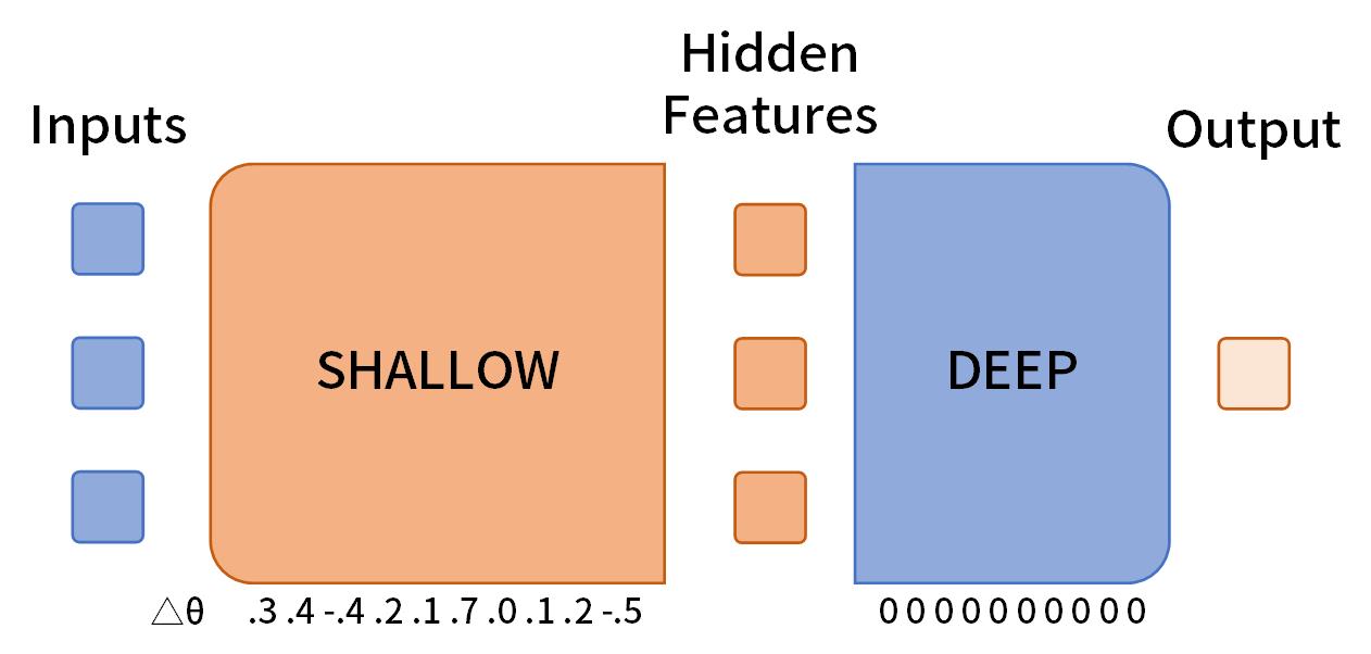
If the trained parameter is a flat minimum, then slight changes in its parameters do not drastically increase loss. Changes restricted to the shallow layers inherit this property. So parameter perturbations that are reflected in hidden features cause no drastic increase in losses. As explained before, the frozen deep layers must have learned implicit adversarial robustness to ensure flatness w.r.t. virtually perturbed inputs for deep layers to mitigate these virtual perturbations to hidden features. This intuition leads to the notion of flat minima and we will follow it in Section 4.3 by proving that both implicit adversarial robustness and some sparsity-related inner products are upperbounded by the measure of flatness, i.e., .
Following this line, one question to answer is how diverse the perturbations are to hidden features. Perturbations to parameters have to go through non-linear operations, which hinders the expressibility of parameter perturbations especially in non-activated neurons. To make things worse, parameter sharing creates hidden features whose dimension is much larger than the parameter that directly produces it, in contrast with explicit adversarial training where perturbations are directly added to in a full-dimensional way. As a result, the perturbation to parameters creates correlated perturbations in hidden features, which cannot cover explicit adversarial attacks that may perturb in an uncorrelated manner. We consider the problem from parameter sharing to be extremely sever in CNN because normally a small () convolution kernel should produce a large feature map. This problem in Transformers is moderate because there are seemingly full-dimensional parameters (e.g. weights and bias in value matrices and MLPs), but tens of tokens are subject to the same parameter so it is low in this token-stacking dimension. Pure MLPs have the smallest problem because its weights and biases are full-dimensional and there is only one token as features, but the perturbations are still subjected to activation functions.
To alleviate these problems through adding non-shared parameters after activation functions, we propose Doubly Biased MLP () by introducing an extra bias or , called zeroth bias (ZB) due to its position, before other operations (so it is after activation functions of previous layers). ZB is a matrix of the same shape with hidden features if they are matrices of stacked tokens, i.e.
| (19) |
where is the zeroth bias of current . For hidden features of single tokens, it writes
| (20) |
For single-token hidden features, the zeroth bias removes the hindering effect of activation functions on the previous layer’s bias , and for matrix hidden features, of the same shape allows full-dimensional perturbations. Note that zeroth biases are added to hidden features, meaning that they share gradients. This property will ease the analyses bridging flatness and implicit adversarial robustness.
Another implication of the above illustration is that activation function matters in gradient and/or activation sparsity, because its derivatives are multiplied when computing gradients w.r.t. hidden features to compute gradient norm that proxies implicit adversarial robustness. In Section 6, we design strange activation to differentiate gradient and activation sparsity and show that activation sparsity is lost to reach gradient sparsity defined by the activation function. On the other hand, one problem of common and is that their derivatives are almost piecewisely constant for most regions, having difficulties in guiding the second-order search for flat minima. By squaring , which coincides with So et al. , the non-constant derivatives of activations provide guidance to sparser neighbors, and -large derivatives for large activations drive the parameters into sparse ones. However, in tentative experiments, we found that the derivatives are too small around zero and provide little drive toward sparsity, so we shift the non-zero parts left and give
| (21) |
where “J” means jumping across the ignored interval and is used to calibrate derivatives at to , approximating ’s and ’s behaviors near . The visualization of , Squared-ReLU and can be found in Fig. 2.
in relu,relu2,jsrelu

One of the benefits of our architectural modifications is that they are plug-and-play, not only for training from scratch, but also for directly loading weights of vanilla architectures with changes plugged in and finetuning for sparsity, given that and can be initialized to for any weights, and approximates or to the first order at . Due to their simplicity, they are also likely orthogonal to other potential methods.
Now we have established the framework of our explanation. A formal analysis following this framework, based on , is conducted in the following three subsections. We will first calculate gradients in MLP blocks. Starting the analyses, we relate flatness to implicit adversarial robustness, and then implicit adversarial robustness to gradient sparsity in Section 4.3. After that, we exclude alternative sources of implicit robustness and flatness. To give the most general form of results, we assume in later subsections, if is not explicitly pointed out. To obtain results for , simply remove the ZB-related term (usually the first term) in inequalities.
4.2 Gradients w.r.t. Weight Matrices and Zeroth Biases
Since we are interested in the flat minima, gradients will be heavily involved. Therefore, we will compute gradients and updates to weight matrices in this subsection. We will also define the notion of effective gradient sparsity and argue its practical and theoretical importance, justifying our theories that are built on effective gradient sparsity.
Let be any sublayer of the block , whose weight matrix is . Let be the gradient w.r.t. the output of on sample at a token , where abstracts , or . Let be the stacked version of and be that of .
One can compute the gradient w.r.t. on a token input by
| (22) |
where for weight matrices, while is for value matrices since there are no activation functions in value layers. Summing updates from all tokens to obtain gradients of sample gives
| (23) |
The gradients w.r.t. zeroth biases, if they exist, are also computed.
| (24) | ||||
| (25) |
Instantiating these results on key and value matrices obtains Lemma .
Lemma 0 (Gradients w.r.t. weight matrices)
The gradients w.r.t. weight matrices and zeroth biases in of sample are
| (26) | ||||
| (27) |
Particularly if hidden features are single tokens, there are
| (28) | ||||
| (29) |
Lemma introduces a Hadamard product between gradients from deeper layers and the derivatives of the activation in weight layers. We define it as the effective gradient pattern.
Definition 0 (Effective gradient sparsity)
Define effective gradient patterns of on sample at token to be
| (30) |
Let (capitalized “” instead of capitalized “”) be its stacked version when there are tokens.
Effective gradient sparsity is that most elements in are near zero for most samples and tokens. For mathematical convenience, define to be the effective gradient sparsity measured in squared norm.
This notion first simplifies Lemma .
Lemma 0 (Gradients w.r.t. weight matrices, restated with and )
The gradients w.r.t. weight matrices and zeroth biases in of sample are
| (31) | ||||
| (32) |
Particularly if hidden features are single tokens, there are
| (33) |
This sparsity inherits sparsity in s but also allows more “sparsity” due to s. Sparsity in is also meaningful in the sense that if the -th entry of is small in magnitude, then 1) there is little contribution of -th neuron in gradients to shallower layers during the backward propagation and 2) does not influence the output much in forward propagation if the activation is also near-zero. Therefore, the -th neuron can also be pruned during backward propagation and possibly during inference with minor cost in accuracy, and thus this notion is of even more practical value, although cannot be known before backward propagation. The notion of effective gradient sparsity in considers the two kinds of sparsity in a combined manner. This incorporation of gradients w.r.t. activations also reminds us of the improved knowledge attribution method proposed by Dai et al. (2022) where not only activation magnitude but also the gradients of model output w.r.t. the activation are exploited. Last but not least, the effective sparsity hides the complexity of deeper layers and attributes its emergence solely to , which is somehow shallow despite there being dozens of deeper modules and allows easier theoretical manipulations.
More importantly, effective gradient sparsity patterns are what key layers try to memorize in columns, given in Observation 1.
Observation 1 (s are memorized in key matrices columns)
Consider the update of one sample to the key matrix given by Lemma
| (34) | ||||
| (35) |
In the update of each column, a mixture of effective gradient sparsity patterns is borne into the key matrix with different weights given by the input.
Taking a transposed view, key layers also memorize s, under the control of s.
Observation 2 (s control row memorization in key matrices)
Consider the update of one sample to the key matrix given by Lemma
| (36) |
In the update of each row, a mixture of inputs is borne into the key matrix, weighted by entries of effective gradient sparsity pattern.
Similar things also happen in value matrices but with s and s memorized. It is interesting to see that linear layers are trying to resemble the gradients back-propagated to them. This observation may lead to a notion of pseudo gradients which can be calculated as the forward propagation sweeps by. Maybe a portion of samples can be trained by these pseudo gradients to save computation budgets. However, this is out of our scope and is left for future works to explore.
Unfortunately, effective gradient sparsity is not strictly related to activation sparsity even under common activation functions, so we keep the notion of gradient sparsity as well. The gap is due to the Hadamard product with , which can cause smaller without gradient sparsity on by 1) reducing the norm of itself, or 2) misaligning itself with , i.e. multiplying small entries in with the derivatives of activated neurons and leaving large gradients to non-activated neurons. The modeling of sparsity also hinders the direct relation with sparsity measured in norms. The first possibility can be eliminated by the phenomenon of parameter growth already discovered by Merrill et al. (2021). This indicates that the norm of Transformers’ parameters will increase even under weight decay and normalization. Since gradients are obtained by multiplying parameters and hidden features, is also likely to increase. We empirically examine it in Section 8.1 where is observed to increase, at least in ViTs. For the second possibility and the disconnection between and norm, under -activation, similarly to Remark , can be seen as the norm of activations, but weighted by entries in . In Section 8.2, we will empirically demonstrate that aligns with very well, i.e., the distribution of squared values of entries in that corresponds to non-zero entries in is similar or even righter-shifted compared to the distribution of all entries’ squared values in , and the former avoids the long tail of the latter with small magnitudes. This indicates that it is not the case that effective gradient sparsity measured in norms is achieved by adversarially aligning non-zero derivatives of activation functions to small gradients and aligning zero derivatives to large gradients. Therefore, the weighting by to the norm is quite moderate, and a considerable portion of - entries in are attached to large weights that can be approximated by (which is increasing under parameter growth), so at least this portion of entries enjoy the approximate connection from effective gradient sparsity to gradient sparsity, and finally to activation sparsity. This intuition leads to Lemma that fully exploits coincidences in and the piecewise constancy of norm.
Lemma 0 (Relation between and for networks)
Let be a set of - vectors and be a set of real vectors. Let , resembling Definition . For any distribution over subscripts , there is
| (37) | ||||
| (38) | ||||
| (39) | ||||
| (40) | ||||
| (41) | ||||
| (42) |
where stands for uniform distribution among , and stand for the -th entry of the -th vectors.
In Section 8.2 we will demonstrate that is comparable to or even larger than that is increasing due to parameter growth. For other activation functions with jump discontinuity between deactivation and activation like , the alignment is also moderate and the weighted norm first pushes activations towards zero, after which norms become closer to norm due to derivatives’ jump discontinuity at . Following a similar argument of Lemma , effective gradient sparsity then approximates sparsity measured in norms as well. Another very informal and heuristic argument for the alignment as well as ’s connection to activation and gradient sparsity is that, if the -th entry in is near zero, then during the row memorization described by Observation 2, little change is imposed by to the -th row of . Next time arrives, although with changes due to shallower layers, it is more likely the -th row in forgets and or are closer to or negative values, leading to smaller possibility of activation, followed by activation sparsity in , and thus gradient sparsity in under common activation functions. To sum up, effective gradient sparsity measured by norm can be connected to activation or gradient sparsity measured in norms, although the result requires empirical assumptions and is heuristic and informal for activation functions other than . Therefore, we will base our theorems on considering the connection discussed above and the mathematical convenience brought by norm and the Hadamard product.
4.3 Flat Minima, Implicit Adversarial Robustness and Effective Gradient Sparsity
As discussed in Section 4.1, we start from and relate it to implicit adversarial robustness w.r.t. some hidden feature , or . Cross Entropy loss is assumed under classification tasks. Note that aside from explicit classification tasks, next-token classification and Cross Entropy loss form the basis for many self-supervision objectives in NLP pretraining, including causal language modeling and masking language modeling. Therefore this assumption can be applied across broad practical scenarios. Assuming , the Hessian writes
| (43) |
which, together with , reminds us of the famous equality of Fisher’s Information Matrix, i.e.,
| (44) |
the trace of RHS of which is exactly the expected squared norm of the gradients. So adapting the classic proof of this equality, we connect flatness measured by Hessian trace to the norm of gradients in Lemma .
Lemma 0 (Flatness and samplewise gradient norm)
Assume is a neural network parameterized by , trained by Cross Entropy loss . Given being the Hessian matrix of loss at , there is
| (45) |
Further for well learned models, i.e., for all training samples, there is
| (46) |
The proof of it can be found in Appendix A. This lemma invokes a samplewise point of view on Hessian and flatness, which is closer to adversarial attacks because they are added in a samplewise manner. Aside from implication in the context of sparsity, Lemma indicates that a flat minimum also provides solutions that are locally good for most individual samples. We acknowledge that similar results with gradient outer products under abstract losses have been given by Sagun et al. (2018), but we believe under Cross Entropy loss the result becomes more direct, intriguing and implicative. As an aside, Cross Entropy seems an interesting loss function, for example, Achille and Soatto (2018) rewrite CE loss expected among all training traces into mutual information between training data and final parameters.
After that, we move perturbations from parameters to hidden features in Lemma .
Lemma 0 (Gradient norm and implicit adversarial robustness)
Let be a neural network parameterized by , and the parameters for the -th layer is . Let be the -th doubly biased MLP in whose input is , zeroth bias is . Then there is
| (47) |
If is not doubly biased, then the first term in RHS simply disappears.
Proof By noticing contains at least and , there is
| (48) |
Consider how is processed in : It is added with before any other operations. So there is .
Combining Lemma for the second and the third terms, the lemma follows.
From the proof of Lemma we can see that zeroth biases avoid tedious linear or non-linear operations and drastically ease our analysis. This implies that one can design theoretically oriented architecture that allows easier theoretical analyses.
We then connect implicit adversarial robustness to gradient sparsity.
Lemma 0 (Implicit adversarial robustness and gradient sparsity)
Under the same condition of Lemma , together with the assumption that in the weight matrix is and is the entrywise derivatives of activations, there is
| (49) |
if hidden features are single tokens, where is a symmetric positive semi-definite matrix of rank at most , denotes Hadamard product, i.e., entrywise product.
If hidden features are matrices, then there is
| (50) |
Proof By Lemma , the gradients w.r.t. is
| (51) |
Similar to the proof of Lemma , and share the same gradient, so
| (52) |
Now we can compute the squared norm of gradients by its relation with trace
| (53) | ||||
| (54) |
To see how emerges, expand the definition of and obtain
| (55) | ||||
| (56) | ||||
| (57) |
where the second last step is to apply Eq. 11. Note that ’s rank is at most .
When hidden features are matrices, sums the gradient norms for all tokens, which leads to
| (58) | ||||
| (59) |
Theorem 0 (Flatness, implicit adversarial robustness and sparsity)
Let be a well-learned neural network parameterized by , trained under Cross Entropy loss . Let be the Hessian matrix w.r.t. parameters at . Let be the -th doubly biased MLP in whose input is . There is
| (60) | ||||
| (61) | ||||
| (62) |
The first term can also be expressed by , where is a symmetric positive semi-definite matrix of rank at most . Further by Schur’s Theorem, is also positive semi-definite.
If vanilla s are used, then the first term in RHS simply disappears.
The chained upperbounds connect flatness and implicit adversarial robustness to effective gradient sparsity (the first two terms in Equation 62) and as well as activation sparsity (the last term in Equation 62), indicating that both gradient and activation sparsity can be sources of implicit adversarial robustness and flatness. If flatness is achieved, then it is possibly done through (effective) gradient sparsity and activation sparsity. Note that this bound is very tight because s take a large portion of parameters (Dai et al., 2022) even in Transformers, so by Cauchy’s Interlace Theorem most large eigenvalues of are retained in the submatrix of parameters. Therefore to achieve flatness, the terms in Eq. 62 must be suppressed.
4.4 Discussions on Theorem
In this section, we discuss the implications of Theorem under several particular settings, including pure MLPs, pure LayerNorm-ed MLPs, Transformers and Transformers with hypothetical massive perturbation training. We point out their tendency toward effective gradient sparsity, which leads to gradient and activation sparsity as discussed in Section 4.2, among which effective gradient sparsity is more stable.
4.4.1 Pure MLPs
The last two terms in Eq. 62 have similar forms, so we inspect them together. To have a clearer understanding on them, first consider the situations where models use single-token hidden features in Corollary
Corollary 0 (Flatness and sparsity in pure MLPs)
. Inherit the assumptions of Theorem . Assume additionally that the model uses hidden features of single tokens, then there is
| (63) |
Proof With single-token hidden features, reduces to
| (64) | ||||
| (65) | ||||
| (66) |
can be reduced similarly.
If normalization layers are imposed, for example, LayerNorm layers before MLP blocks, then will not change during training, eliminating all other sources of suppressing the second term aside from effective gradient sparsity.
Since key matrices also take a large portion of parameters, flatness in these parameters must be achieved as well and is not too small from , the second term alone will have a strong tendency to decrease. Therefore, a rigorously proved, strong and stable tendency of pure LayerNorm-ed MLPs toward effective gradient sparsity is presented in Theorem .
Theorem 0 (Flatness and sparsity in pure MLPs with LayerNorms)
Inherit the assumptions of Theorem . Assume additionally that the model uses vector hidden features and LayerNorm layers, with affine transformation turned off, are imposed before every MLP block. Temporarily assume non- models are used, then there is
| (67) |
If s are used and LayerNorm layers are placed before zeroth biases, by clipping the norm of columns in zeroth biases to , there will be
| (68) |
By Lemma , for networks, there is further
| (69) | ||||
| (70) |
for networks, and similar results can be obtained for architectures without zeroth biases.
LayerNorm places quite strong and stable drives towards effective gradient sparsity, if they are placed right before (DB-)MLP blocks and affine factors are turned off to avoid their reduction due to updates or weight decay. Theorem can be one explanation of the benefits of LayerNorms and the practice to exclude their parameters from weight decay.
The last term in Eq. 63 relating activation sparsity is less ensured than the second term. In experiments (although conducted with Transformers) we observe becomes small in deep layers, indicating that effective gradient sparsity is the main cause of activation sparsity in deep layers.
4.4.2 Transformers and Other Architectures
When stacked hidden features are used, for example in Transformers, the discussion is more tricky. It is possible that gradients of different tokens cancel each other in
| (71) |
We can only rigorously conclude a possibly loose lowerbound with in Corollary using Eq. 10.
Corollary 0 (Flatness and sparsity in Transformers)
Inherit assumptions from Theorem , then there is
| (72) | ||||
| (73) | ||||
| (74) |
where indicates the minimum eigenvalue of a matrix.
Proof
| (75) | ||||
| (76) |
The last term can be similarly rearranged. Applying Eq. 10 to both of them and noticing finish the proof.
There are tricky ways to bypass the canceling, however. For example, consider augments conducted on hidden features such as dropout. They effectively duplicate the parameter into views and perturb each view independently (using dropout, rows of weight matrices are randomly pruned) if there are tokens. If flatness can be extended to these effective duplicated parameters, i.e., if there is still flatness when we really duplicate the weight matrices and assign one token for each matrix, then each view is only handling one token and we can repeat Corollary . However, traditional dropout may hinder the sparsity by eliminating activations and forcing the model to back up the representation. Additionally, its perturbations are not local enough, hindering theoretical analyses. A soft dropout by slightly perturbing before activation functions is more preferable. Moreover, the perturbation should better be conducted on weight matrices in an entrywise manner to avoid summing and canceling gradients. Under this hypothetical synapse perturbation (Murray and Edwards, 1994, 1993) but in a tokenwise manner, we assume flatness can be obtained w.r.t. the duplicated parameters because, in the real model, losses are suppressed even under independent perturbation so the effective model is not sensitive to independent changes in individual parameter duplicates. This intuition leads to Lemma .
Lemma 0 (Flatnesses of perturbed model and perturbation-induced effective model)
Assume weight matrices are perturbed by Gaussian noise independently for each token, i.e., the perturbed outputs
| (77) |
for input hidden matrix , where , and are independent centered Gaussian variables with variance . Let random variable denote the collection of all perturbations. Let be the collection of proxied parameters, where s are taken into consideration instead of , while other parameters are inherited from .
Let be the effective parameter by duplicating each weight matrix for times into , each of which deals with exactly one hidden vector during inference.
Then
| (78) | ||||
| (79) |
where indicates the loss of on sample when perturbation is , is the number of layers. If Cross Entropy loss is assumed and is well learned when perturbations are removed then by Lemma applied to ,
| (80) | ||||
| (81) | ||||
| (82) |
Proof By construction of , gradients w.r.t. and share the same path in and . If the same sample is used and the perturbation is removed, then they are equal.
We can approximate from by
| (84) | ||||
| (85) |
Since Gaussian has covariance , is also Gaussian whose variance is
| (87) |
Taking expectation over noises , there is
| (88) | ||||
| (89) |
where denote the collection of all s.
The rest of the proof is easy according to the equivalence between with perturbations removed and .
Remark 0
Although is involved by an inequality, considering the large portion of parameters, can in fact represent well. If this argument is not satisfying, then perturb all parameters in the same way so that “” becomes “”.
So by training a weight-perturbed non-pure-MLP network to have low losses, we are helping its pure-MLP equivalence reaching flat minima, where effective gradient sparsity can be directly obtained in Theorem . If we assume
| (90) |
is indeed suppressed during training because losses are suppressed to near-zero values, then Theorem is meaningful.
Theorem 0 (Flatness and sparsity under tokenwise synapse noise perturbations)
Inherit the assumptions of Theorem as well as notations in Lemma . Further assume that weight matrices are independently perturbed before multiplying with any individual tokens during training, then
| (91) | ||||
| (92) | ||||
| (93) | ||||
| (94) |
where stands for the perturbation-induced effective parameter where weight matrices are really duplicated so that each of them serves one token and is the collection of parameters in all zeroth biases. If no-affine LayerNorms are applied, there is further
| (95) | ||||
| (97) | ||||
| (98) | ||||
| (99) |
where if non-s are used, otherwise is the norm bound of columns in zeroth biases.
By Lemma , for networks, terms in the above equations can be replaced by to have a direct relation with activation sparsity.
Aside from Transformers, tokenwisely perturbed CNNs, channel mixing layers of MLP-Mixers and other potential architectures apply, as long as they have MLP blocks and the perturbed loss is small enough. Additionally, this bound is also very tight by the tightness of Lemma or by counting parameters, so perturbed error’s reduction or the flatness of the effective model inevitably leads to a reduction in sparsity. A simple algorithm is immediate after Lemma and Theorem , which is listed in Appendix F in order not to disrupt the presentation of major theoretical results.
4.4.3 The First Term from Zeroth Biases
Now we look back to the first term in Eq. 62. Although the first term seems to have minor weight compared to others, either by counting parameters or by decomposing eigenvalues of (see Fig. 13(a)), an investigation is still worthy since it leads to another phenomenon of spectral concentration in and introduces random matrix theory to reason about training dynamics.
In the first term, since the gradient of the inner product w.r.t. is
| (101) |
there is an overall positive tendency toward sparsity if is suppressed, because is non-negative, i.e., partial derivatives w.r.t. are always overall positive if they are weighted by values in themselves.
It is better to reach a non-overall conclusion. Moreover, there are two possibilities that can also achieve implicit adversarial robustness: reducing the norm of , or misaligning the non-null space of with . The first alternative can already be eliminated by parameter growth observed by Merrill et al. (2021), where Transformers are observed to have increasing parameter norms during training. We also empirically verify this phenomenon under CV and NLP settings and show that the trace, or the sum of eigenvalues, will not decrease drastically during training in Section 8.1, even under weight decay. Another possible elimination is normalization layers, which make parameters scale-invariant and introduce normalized effective parameters (Zhang et al., 2018) with moderate norms. However, this requires a total reform of the theory to utilize effective weight matrices so we simply hide normalization layers in and leave it, and especially its interaction with weight decay, for future works.
The other alternative is dealt with in the next two subsections, where single-token features are used in proofs but the theories apply to stacked hidden features. To give a brief account, in the following subsections we will prove that non-zero eigenvalues of have similar values. So if gradients have moderate projections in the non-null subspace of , then can be lowerbounded by , where indicates how much of falls in the non-null space of and is the smallest non-zero eigenvalue or some averaged non-zero eigenvalues of , which is not too small compared to the largest one. Assuming gradients are still back-propagated to shallower layers, can only be suppressed by decreasing given that increases with the trace of . In Section 4.5 we prove this phenomenon at initialization in Theorem that the largest eigenvalue is initially at most times larger than the smallest non-zero one in Base-sized Transformers. The proof is based on ubiquitous Xavier or Kaiming initializations and Marchenko-Pastur distribution from random matrix theory. In Section 4.6, we theoretically discuss its re-emergence during stochastic training. We first rewrite the updates to the weight matrix into two large random matrices, whose shape is hidden dimension times the number of samples used in training. We then extend Marchenko-Pastur distribution in Theorem under the practical inter-batch dependence, intra-batch independence and non-asymptotic scenario to prove an upperbound on the fraction between the largest and smallest non-zero eigenvalues. Conditions and assumptions of the theorem are verified empirically in Section 8.5. There are still gaps in combining the two random matrices, so we measure the spectral concentration in empirically in Section 8.4 and leave a more rigorous discussion for future works.
4.5 Spectral Concentration at Initialization
In this section, we prove that has eigenvalues that are close to each other, at least at initialization. With effective gradient sparsity measured by , this spectral concentration allows us to approximate the first term in RHS of Eq. 62 with , which is almost directly effective gradient sparsity measured in norms.
To reach this goal, recall Marchenko–Pastur distribution in Theorem that reveals the asymptotic spectral distribution of random matrices’ product. Applying Theorem to initialized by Xavier or Kaiming initialization, we obtain Theorem .
Theorem 0 (Initial spectral concentration of )
Assume . Let be the weight matrix initialized by (Gaussian, uniform, or other distribution-based) Xavier or Kaiming initialization. When with , the ratio between the largest and smallest non-zero eigenvalues of converges weakly to
| (102) |
Regarding zero eigenvalues, if , there is no zero eigenvalue, and if , the expected portion of zero eigenvalues is .
Proof The initialization methods utilize centered distribution, and thus there is .
differs from of Theorem in 1) the shared standard variance of entries not being , and 2) the scaling factor . Since we are only interested in the ratio between eigenvalues, these differences of simultaneous scaling can be ignored.
By Eq. 18, we can see that the support of eigenvalues is restricted to . As a result, non-zero eigenvalues can only be found in .
When , i.e., , the support degenerates to .
When , the probability to pick a zero eigenvalue is .
Note that Theorem applies to uniform or other base initialization distribution as long as it is centered and entrywisely independent with the same variance. Since are generally large, even in small model sizes like Small and Base, we believe this lemma applies to common practice. In Base-sized Transformers, it is usually the case where , indicating of eigenvalues are , while the rest of them varies up to the ratio of . This is a surprisingly small value compared to the number of dimensions.
Effective gradient sparsity patterns have a great affinity to , allowing Theorem .
Theorem 0 (Implication of spectral concentration of at initialization)
Assume and they are sufficiently large. is initialized as in Theorem . Let , and be those defined previously.
If then there is
| (103) | ||||
| (104) |
where -th eigenvalue is moderate and cannot be arbitrarily small because
| (105) |
where .
If , let be the singular value decomposition of . The result is restricted to the projection to the subspace expanded by , i.e.,
| (106) | ||||
| (107) |
where -th eigenvalue satisfies
| (108) |
where .
For demonstration, when , the ratio upperbound is .
Proof
The proof is straightforward after Theorem , by noting that when there are exactly zero eigenvalues in , or equivalently non-zero eigenvalues in .
There are still gaps between and current practices where and there are a lot of zero eigenvalues in , but Theorem is perfectly useful for wide MLPs where . Therefore, we propose a drastic architectural modification called wide MLP where , i.e., the model dimension is larger than the hidden dimension in MLP blocks. Aside from more powerful motivation toward sparsity, wide MLPs also allow rows in to be mutually orthogonal and permit perfect sparsity, which is impossible when .
In non-wide MLPs, we believe that since are randomly initialized and samples are randomly selected, there are moderate projections of into the non-null subspace of . Another supporting intuition is that although is not identity or linear, the derivatives of common activation functions are often monotonically increasing and form an approximation to its inputs. This approximation is better when part of the activation derivatives are linear, as in the case of Squared-(So et al., ) and our . Therefore, taking to , which already falls near the subspace expanded by , does not deviate far from the subspace. Observation 1 also supports this moderate projection dynamically because if is in the null space, it will be borne into every column of the key matrix and next time it will have non-zero projections if does not change too much after one epoch and the column memory is not blurred too severely. Repeatedly memorizing different will make the non-null space of a mixture of the majority s provided by the training data set. The empirical evidence for this is that , according to the derivation in Lemma , is actually the norm of gradients back propagated to shallower layers. Extreme cases where are contained only in the null space of result in zero gradients for shallower layers, which rarely happens. If no residual connection is involved this insight strongly augments the spectral explanation. The detailed and formal analysis of the zero eigenvalues especially when there are residual connections is left for future empirical and theoretical works. For now, we can simply cover the gap with wide MLPs.
4.6 Spectral Concentration during Stochastic Training
In this subsection, we discuss how spectral concentration re-emerges during later stochastic training.
First recall the Marchenko-Pastur distribution in Theorem . The condition of random centered matrices in Theorem invites another randomness other than initialization to the party, i.e., stochastic gradient noise (SGN) brought by stochastic optimizers. After updates, can be written as the sum of random initialization, stochastic gradient noises and full-batch gradients that are not as stochastic as the two former terms, i.e.
| (109) |
As discussed in Section 3.4, is by definition centered. If it can be assumed that the SGN with large variance and noise norm shadows full-batch gradient, then is the sum of two centered random matrix with a slight non-stochastic bias, to which Marchenko-Pastur distribution would approximately apply if further entries in shared similar variance and were sampled independently. Bryson et al. (2021) and works cited by them have tried to relax the independence condition of Theorem , but it is still far from applying relaxed Marchenko-Pastur distribution here. Aside from waiting for this mathematical progress, we build empirical basis in Section 8.4 where at all steps, in of ViT and the decoder of T5, there is a stable portion of near-zero eigenvalues as in Theorem across all layers, and the majority of non-zero ones, with significant gap with near-zero ones, vary up to a ratio of for most of the time. It is not surprising that this effect empirically sustains and even becomes stronger at the end of training because the model is well-learned by then and the full-batch gradient is of a smaller norm.
To have a more satisfying discussion, we propose an extended version of Marchenko-Pastur distribution and find a re-directed view on stochastic gradients to apply it. To this end, what conditions and assumptions can stochastic training provide must be figured out first.
Observing the structure of or layers, the most essential operation involving weight matrix is
| (110) |
where is abused to represent anything that is multiplied with , abstracting or , while is the vector passed to the vanilla bias, activation function or later layers. This structure gives birth to the update of a sample to that writes
| (111) |
where is the learning rate, assuming no scheduling is used. At step with batch , the update on averages these samplewise differences, i.e.
| (112) |
where (capitalized “”) is the matrix consisting of column vectors for sample in the batch , and is similarly constructed with . Note that and are random matrices because samples are independently randomly selected and gradients are also random variables as functions of variables. Taking a similar view throughout the training, there is
| (113) |
where is the number of batches, is batch size, and , and . Another product of large random matrices emerges in the empirical covariance matrix of the difference, i.e.,
| (114) |
where and are random matrices in the sense that samples or gradient vectors in each batch are independently randomly sampled, if conditioned on the model state.
Since we are interested in spectral distribution and that cycling a matrix product does not change non-zero eigenvalues, a more desirable form is
| (115) |
and we intend to separately investigate the spectral distributions of
| (116) | ||||
| and, | (117) |
After these transforms and dividing-and-conquering, the empirical covariance matrices look ready for Marchenko-Pastur law. However, there are dependencies between previous and later batches through model states, hindering the direct application of independence conditions of Marchenko-Pastur law. Fortunately, there is still conditional independence within a batch. This mixture of dependence and independence is captured by Definition .
Definition 0 (Batch Dependence Model)
Let be a random matrices. Decompose it into blocks with batch size , i.e.,
| (118) |
where . If the dependence between elements can be described by SCMs
| (119) |
or SCMs that resemble the notions of samples and model state
| (120) |
where s are columns in , is the model state (parameters, momentum, etc.) after step , is I.I.D. random noises, then is a random matrix with batch dependence.
Remark 0
Within each batch (i.e., when conditioned on all previous batches), samples are I.I.D. sampled to simulate batch sampling. However, previous samples have trained the parameters and will shift the distribution of shallow layers’s output as well as back-propagated gradients. Therefore, the current batch depends on previous batches.
There are works re-establishing Marchenko-Pastur law with independence conditions relaxed to martingale conditions (Gotze and Tikhomirov, 2006), but some conditions in it require entrywise conditional independence. There are also Marchenko-Pastur laws for time series (Yao, 2012; Liu et al., 2015), but restricted to linear dependence. We adapt proofs by Yaskov (2016), and use anisotropy condition in all samples or gradients to extend Marchenko-Pastur distribution under the batch dependence in and , leading to Theorem . In later formal definitions, theorems and proofs, is abstractly used to represent both or , indicates the height of or , i.e., the hidden dimensions or , while and keep their meanings as batch size and total number of batches.
Theorem 0 (Spectral concentration of accumulated steps)
Let be a random matrix that forms a Batch Dependence Model as in Definition with batch size and step count , whose columns are . Columns in are not necessarily independent.
Let be the -th column of and be the -th column of batch or equivalently the -th column in . Superscription may be dropped for convenience.
Let be the empirical covariance matrix of all random vectors, and be the compatible identity matrix. Assume s’ norm is bounded, say by , and scale it with
| (121) |
obtaining , where . Let
| (122) |
be the empirical covariance matrix of all s.
Assume is bounded by and is also upperbounded by .
Further assume that the following function of and
| (123) |
is always continuous w.r.t. for any .
If the above assumptions are satisfied, the non-zero eigenvalue concentrates. To be more specific, let be the mean of non-zero eigenvalues of and use to represent the overall situation of non-zero eigenvalues. Then there is
| (124) | ||||
| (125) |
for any , where is a randomly selected eigenvalue of and , and satisfying
| (126) |
with .
Its proof is left in Lemma . This concludes that spectral concentration also happens in and , as long as the samples in one batch are independently sampled and all model-state-specific samples involved during training are diverse enough to have low anisotropy and norm bounds. To see that the conditions are satisfied, note the only hard conditions are that of continuity, which is hard to verify and thus simply assumed, as well as the choice of and . We assume enough steps have been trained so can be very small, for example effectively under strong weight decay (it is even smaller when weight decay weakens or disappears) as we shall see in latter paragraphs. So can be chosen. In experiments in Section 8.5 we will see is always smaller than and can be less than when weight decay is strong and dimension is large enough. Under these conditions, it can be verified that LHS of Eq. 126 is larger than RHS by at least . So the applicability of the theorem depends on how good the bound is. To empirically verify the applicability of Theorem , one needs to compute anisotropy and from ’s marginal distribution, i.e., by mixing hidden features or back-propagated gradients, which is conducted in Section 8.5.
In contrast with conventional asymptotic results with and in RMT, our theorem gives bounds for non-limiting scenarios. One of its benefits in the context of machine learning is that one often is more interested in training behaviors when the total number of training samples increases as the training proceeds while is held still. Nevertheless, the co-increasing scenarios are also of interest, especially in the era of large models (Kaplan et al., 2020). In our result, the spectral concentration is measured by the expected fraction between eigenvalues and the expected eigenvalue, but with an extra shadowing parameter that may shadow small eigenvalues and decreasing to suppress the disturbance loosens the bound. Fortunately, most as dominators show up together with as numerators, the ratio between hidden dimension and number of training samples used which is often extremely small. If is also small and decreases as is enlarged, as we will show in the experiments, then the bound will be controlled.
It is frustrating to see that the bound diverges as the training step increases due to factor . However, we consider weight decay as an alleviation to this issue. Weight decay effectively introduces a sliding window which reduces the effective , because vectors out of the window are exponentially decayed and they have little contribution to the sample covariance matrix. For example, let be the parameter of weight decay, then each column in or becomes or , where is learning rate. Setting , if we consider the tail whose weights’ sum is smaller than a threshold as those out of the window, then the window size needs to satisfy , where is used to obtain tighter bounds instead of by arguments in Appendix D. One sufficient condition for this is . When , the effective window size is about . When increases to , the effective window size becomes . As a result, is upperbounded by a constant as the training proceeds if weight decay presents.
There are still gaps between our results and the spectral distribution of during stochastic training. For example, spectral concentration of and hints similar phenomena in their interlaced product , which, however, is not yet formally proved. Moreover, applying Theorem assumes SGD instead of adaptive optimizers is used due to Eq. 113. Filling these gaps is left for future works because we have established spectral concentration’s empirical supports in Section 8.4.
Finally, we have discussed the spectral concentration of . To put everything together, assuming moderate projection of into non-null space of , and considering the increasing trace of and spectral concentration in , the only way to suppress
| (127) |
is to reduce . To see gradient-sparsity-induced activation sparsity’s emergence, given empirically that will not decrease during training, the only way to suppress is to decrease , at least at entries where has large magnitudes.
5 Refined Zeroth Biases
After the analyses in Section 4, the use of zeroth biases proposed in Section 4.1 can be further refined. Theorem and Theorem emphasize the role of LayerNorm layers in sparsity. To push sparsity further, it can be beneficial to enforce a lowerbound of elementwise scaling factors of LayerNorms.
The two theorems also hint at conflicts of LayerNorm with zeroth biases and elementwise biases in LayerNorm. Therefore, one can turn off the elementwise biases in LayerNorm layers and then confine the norm of columns in zeroth biases. We choose to simply clamp the parameter of zeroth biases. To utilize the potential rising of elementwise scaling factors, the upperbound of absolute values of zeroth biases are determined relatively to the elementwise scaling factors. Putting things together, we execute Algorithm 1 after every update during training from scratch.
In sparsity finetuning, it is not likely that the loaded checkpoints have scaling-restricted and unbiased LayerNorms so we freeze LayerNorms’ biases and gradually uplift the absolute value of scaling factors while retaining their signs after each update according to Algorithm 2 instead of RestrictLayerNorm. It is also possible that changing to without any adaptation harms the performance, so we mix and linearly and increase the portion of linearly after every step, starting from . Section 7.2 shows that the refinement performs well during finetuning.
6 Experiments for Verification
The experiments for verification are designed to rule out other possible explanations and show that gradient sparsity is the main cause of activation sparsity, at least in .
Although comprehensively demonstrated by Li et al. (2022b), the sparsity emerging in MLP blocks has still a lot of confusion. This is because a lot of coincidences exist in . For example, and its derivatives share the same zero-valued intervals, and they are both monotonically increasing. Previous works (Li et al., 2022b; Andriushchenko et al., 2023a) consider that it is the value or norm of activations that are reduced to produce sparsity. There are more possible explanations, such as the absolute value of activations as well as all similar explanations based on pre-activations. We show none of them is the essential source of observed activation sparsity but the gradient sparsity, by designing weird activation functions, using which activations or pre-activations are not consistently decreased, increased or moved towards zero, but the norm of derivatives is.
Our construction includes an activation function and 4 shifting operations. is defined as
| (128) |
where is a hyperparameter. and its derivatives are illustrated in Fig. 3(a). We shift it around along - or -direction, i.e., use in MLP layers, to decorrelate between activations and pre-activations, values and absolute values or norms. If gradient sparsity is indeed essential, then the activations and pre-activations will concentrate around the flat area instead of zero point or any half-planes and will follow it well if it is shifted in another way. To have enough space for all pre-activations, we choose , i.e., the width of the flat area is , which is approximately the width of majority pre-activations in Fig. B.2(c) of Li et al. (2022b)’s experimental observations. To exclude flat area from zero point, we shift horizontally and vertically by . This family of shifted is illustrated in LABEL:fig:shifted_weird0--LABEL:fig:shifted_weird-0. From theory, we expect that most pre-activations and activations will fall around .
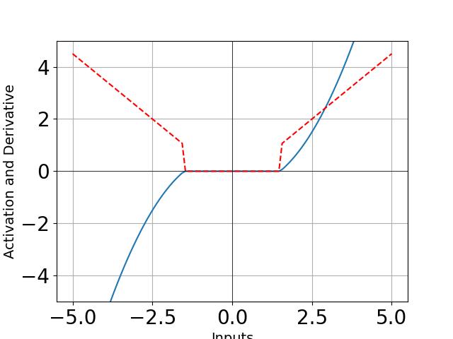
ıin ,- \foreachȷin -,

We train ViT-Base with and on CIFAR-10 (Krizhevsky et al., 2009) for 100 epochs. Training details are listed in Appendix E. The gradient sparsity during training, measured simply by the percentage (Li et al., 2022b) of activations not falling in , is illustrated in Fig. 4.
ıin +,- \foreachȷin -,+

In Fig. 4, most layers have at least 70% activations concentrating at the flat area as expected, which not only indicates that activation is currently not sparse, but also is a strong evidence that gradient sparsity dominates the sparsity among other potential factors. Fig. 4 rules out the dominance of other potential activation or pre-activation explanations, because in LABEL:fig:validational_full+0+, LABEL:fig:validational_full+0- and LABEL:fig:validational_full-0+ activation or pre-activation are not decreased, in LABEL:fig:validational_full-0-, LABEL:fig:validational_full-0+ and LABEL:fig:validational_full+0- activations or pre-activations are not increased, while in all of them activations or pre-activations’ norms are not optimized toward zero. Furthermore, in Fig. 4, where the spurious correlation between activation and gradient sparsity is broken, activation sparsity is gone while gradient sparsity survives and follows the expected area well, indicating that gradient sparsity is more stable and can be more essential than the activation one and thus deserves more research attention.
7 Experiments for Productivity
In this section, we conduct experiments with non-weird activation functions on larger data sets to examine the effectiveness our modifications and verify the theoretical guidance behind them. Aside from modified models, vanilla ViTs are used as baselines. Since it is hard to define (or to achieve) sparsity on activations (Li et al., 2022b), even in “vanilla” ViTs, are used throughout this section.
7.1 Training from Scratch
Although distinguished in Section 6, gradient and activation sparsity should better coincide to allow aggressive dynamic neuron pruning during both training and inference. To show their effectiveness in such practical scenarios, we test our modifications of and non-weird by training from scratch ViT-Base/16 (Dosovitskiy et al., 2020) on ImageNet-1K (Deng et al., 2009) and T5 on C4 (Raffel et al., 2020), representing computer vision and natural language processing tasks as recommended by Liu and Wang (2023).
We generally follow PyTorch’s recipe(PyTorch, 2023) for ViT-Base/16, except that we turn off model EMA to avoid deepcopy that bothers experiment tracking and parameter clamping. For major hyperparameters, we use learning rate , weight decay , batch size , cosine annealing scheduler and a variety of random data augmentation during the 300-epoch training. To train T5, we follow major hyperparameters released by Li et al. (2022b) such as learning rate of , batch size of and inverse square root scheduling with linear warmup of 10,000 steps, while filling not mentioned ones from Huggingface (2023). The training of T5 lasts for only 100,000 steps as well (Li et al., 2022b), since it involves too much computation. To make both models sparser, we modify them by plugging zero-initialized zeroth biases before MLP blocks and replacing all with . We run Algorithm 1 after each step with , i.e., . Since a lot of statistics are computed which slows the training, for ViT the logging (including training losses, sparsity, etc.) happens after per-epoch evaluation or every 100 steps in training. The encoder-decoder architecture and larger token number of T5 cost more memory use, so half of a batch is used to compute the statistics. As compensation logging happens every 25 steps for T5. T5 and ViT are both trained for only one trial due to our limited computation budget. More details of the experiments can be found in Appendix E. The training and testing sparsity of ViT-Base/16 and T5-Base are illustrated in Fig. 5 and Fig. 6, and are summarized in Table 1 and Table 2.


| Training Sparsity | Testing Sparsity | Acc@1 | Acc@5 | |||
|---|---|---|---|---|---|---|
| Vanilla | ||||||
| Modified | ||||||


| Training Sparsity | Testing Sparsity | Testing Loss | |||
|---|---|---|---|---|---|
| Vanilla | |||||
| Modified | |||||


Visually obvious significant improvements in activation/gradient sparsity can be found in the experiment results. By integrating the training sparsity along steps, a training sparsity improvement of approximately 50% is achieved in both CV and NLP tasks. By observing the testing sparsity of the last checkpoint, there is a testing improvement of relatively at least 36%. Fig. 5(d), Fig. 5(h), Fig. 6(f) and Fig. 6(l) suggest that sparsity improvements happen in shallow and middle layers of both encoder and decoder. We conjecture that it is because our improvement focuses on stimulating gradient sparsity, which is poorly trained since fewer parameters lie before shallow layers and implicit adversarial samples are insufficient. Zeroth biases can fix this insufficiency. In contrast, deep layers have sufficient implicit adversarial samples but the motivation directly toward activation sparsity is limited, which our modification hardly helps. In Table 1 and Table 2, in contrast to sparsity generalization brought by vanilla training one can observe sparsity overfitting after modification in both CV and NLP tasks. Fortunately, it is slight compared to the improvement.
The improvement in sparsity does not harm performance or generalization. According to Table 1, Table 2, Fig. 7(b) and Fig. 7(d), testing accuracy of ViT only suffers an acceptable accuracy degeneration while the testing loss of T5 surprisingly improves after modification. Nevertheless, the training of the modified ViT indeed slows during the middle stage in Fig. 7(a) and Fig. 7(b), but the lagging diminishes at the end of training. The reason for this catching up remains mysterious and we conjecture it has something to do with the decayed learning rate. For T5 the modified version always have better training and testing losses. Notably, the modified T5 seems to have better generalization because in Fig. 7(d) modified T5 has significantly lower testing losses despite similar training losses with the vanilla one according to Fig. 7(c).
7.2 Finetuning for Sparsity
Apart from training from scratch, we finetune existing weights for sparsity to show a cheaper way to make them sparser, given that our modification is nearly plug-and-play as analyzed in Section 4.1. We use the vanilla weights from Section 7 and finetune it for another 15 epochs or 10,000 steps after applying the modification. Since finetuning is relatively short and mainly serves inference, we only measure testing sparsity rather than training sparsity in this subsection.
LoRA is used for finetuning to modify weight matrices while keeping learned knowledge, because we observe difficulties in recovering performance with full-parameter finetuning in tentative experiments. In both tasks, we use a relatively large for LoRA because we expect better sparsity requires massively rearranging the matrices. LoRA is applied at all matrices in MLP blocks as well as in self-attention blocks. For ViT we directly plug zero-initialized zeroth biases before MLP blocks and replace for , which does not harm testing accuracy thanks to the derivative calibration of to imitate . However we find T5 hard to directly adapt to , so we mix two activation functions linearly and increase the portion of linearly after each step, starting from to during the first 3,000 steps. In tentative experiments we find clamped scaling factors in LayerNorm layers critical to better sparsity, so we apply Algorithm 2 after every step with in both CV and NLP tasks. The finetuning lasts for 15 epochs for the CV task while 10,000 steps for the NLP task. All other hyperparameters are inherited from Section 7.1. The testing sparsity of modified models is compared in Fig. 8, Fig. 9 and Table 3 with those before finetuning and those after vanilla finetuning.


| ViT-Base/16 on ImageNet-1K | T5-Base on C4 | |||||
|---|---|---|---|---|---|---|
| Testing Sparsity | Acc@1 | Acc@5 | Testing Sparsity | Testing Loss | ||
| Before Finetuning | ||||||
| Vanilla | ||||||
| Modified | ||||||
For ViT, the finetuning damages both testing sparsity and accuracy. However, modified finetuning still has advantages over vanilla LoRA finetuning in sparsity so it seems the drop is mainly due to finetuning. For T5 the improvement is significant. After finetuning for sparsity, T5 obtains similar testing sparsity compared to training for sparsity from scratch, indicating that existing language models can become sparser at a relatively low finetuning cost. This sparsity improvement only brings 0.02 degradation in testing loss. Despite the success of finetuning for sparsity in the NLP tasks, training for sparsity from scratch is still recommended for new models because it brings better testing sparsity as well as potential significant reduction in training costs from better training sparsity. In ViT, sparsity improvement mainly happens in shallow and middle layers as illustrated in Fig. 8(d), which can be explained in a similar way as Section 7.1. For T5 the result is more interesting. According to Fig. 9(f) the sparsity improvement mainly happens in decoder layers. This may be related to architectural differences between encoders and decoders, which is of interest to investigate in future works.
7.3 Role of LayerNorm Layers
Although the experiments reported above are conducted with restricted or uplifted LayerNorm layers, we also conducted tentative experiments before these refinements. The results are not displayed in this manuscript due to length limit. Without restricted LayerNorm, ViT has only about relatively 20% sparsity improvements when trained from scratch, and with frozen not-uplifted LayerNorm, sparsity rarely changes during finetuning ViT from vanilla checkpoint whose scaling factors are observed very small. Both theory and experiments indicate the critical role of LayerNorm layers when it comes to sparsity. Last but not least, Li et al. (2022b) observe that there is no activation sparsity in token mixing layers in MLP-Mixer. They attribute it to the small token-stacking dimension. Here based on the theoretical and empirical findings, we provide another conjecture that it is because MLP-Mixer does not have immediate LayerNorm layers before token-mixing MLP blocks (Tolstikhin et al., 2021), but with transposition lying in between.
8 Empirical Supports for Assumptions
In this section, evidence of assumptions required in Section 4.5 and Section 4.6 is empirically examined. The observations are taken during or after training from scratch or finetuning described by Section 7.
8.1 Spectral Increase in and
The traces of and during training from scratch of ViT and T5 are displayed in LABEL:figure:spectral_increase_ViT and LABEL:figure:spectral_increase_T5, respectively.
in ViT, T5
in sparsified, vanilla \foreach\matrixtypein kkT, M

In LABEL:figure:spectral_increase_ViT, both modified and vanilla ViTs have increasing and that increases rapidly first and decays slowly. Note that the decay in the late phase of the training does not directly conflict with the assumption of theoretical results because the sparsity improvements of both modified and vanilla ViTs happen mainly in the early stage of the training, where main sparsity improvemnts happen as well according to Fig. 5. As a result, better implicit adversarial robustness and flatness cannot be obtained by shriking or . Intriguingly in LABEL:figure:spectral_increase_T5 for T5, and swap their roles. drop rapidly first and then stables. This indicates that although decreases flatness can also be parallelly obtained through sparsity.
8.2 Moderate Alignment in between and
Section 8.1 have demonstrated that is not decreased by decreasing , at least in ViT. To bring and closer, we further demonstrate that decreased is not done by adversarially misaligning with , i.e., multiplying gradients of large magnitudes with derivatives of non-activated neurons and leaving gradients of small magnitudes to activated neurons.
We load checkpoints after training models on ImageNet-1K or C4, as described in Section 7. For each checkpoint, we randomly select one batch of samples (2048 samples for ImageNet-1K or 256 samples for C4) to simulate batches encountered in training and use backward propagation to compute , gradients w.r.t. activations, at all layers. The layerwise distribution of squared entries in after mixing all samples, tokens and entries together, as well as the distribution conditioned on activated neurons, is displayed in Fig. 11(a).
In Fig. 11(a), we observe that for most layers, activated neurons have gradients with a distribution similar to the distribution of all gradients. Furthermore, the former is even more concentrated, shorter-tailed and righter-shifted than the latter, in both ViT and T5 of both vanilla and modified architectures throughout training. This moderate alignment indicates that there is no adversarial misalignment in and a considerable portion of entries in have weights from that are relatively large and can be lowerbounded or approximated by . Specifically under -activation, Lemma is made meaningful, since is close to or even larger than (see LABEL:fig:alignment_ratio_imagenet1k_vanilla and LABEL:fig:alignment_ratio_T5_vanilla) for most layers, so the former cannot be reduced since the increase in the latter at least in ViT as observed in Section 8.1, and the only way to reduce effective gradient sparsity measured in norms is to improve gradient or activation sparsity directly measured in norms. As a result, our -based theories are tightly related to activation sparsity measured in norm for networks and are approximately related for networks.
in sparsified,vanilla
\foreachıin 100,150,200,250,299
\pgfmathtruncatemacro\epochid1+ı


in sparsified,vanilla
\foreachıin 20000,40000,60000,80000,95000
in imagenet1k,T5 \foreach\modelin sparsified,vanilla
8.3 Contribution of Gradient Sparsity and Direct Activation Sparsity
Theorem , Theorem and Theorem indicate that gradient sparsity and activation sparsity together lowerbound the implicit adversarial robustness and flatness, with coefficients of and empirically. To provide support for our emphasis on gradient sparsity, we compare and . Since scaling factors are controlled and tracked only in modified models, only results from modified training are provided.
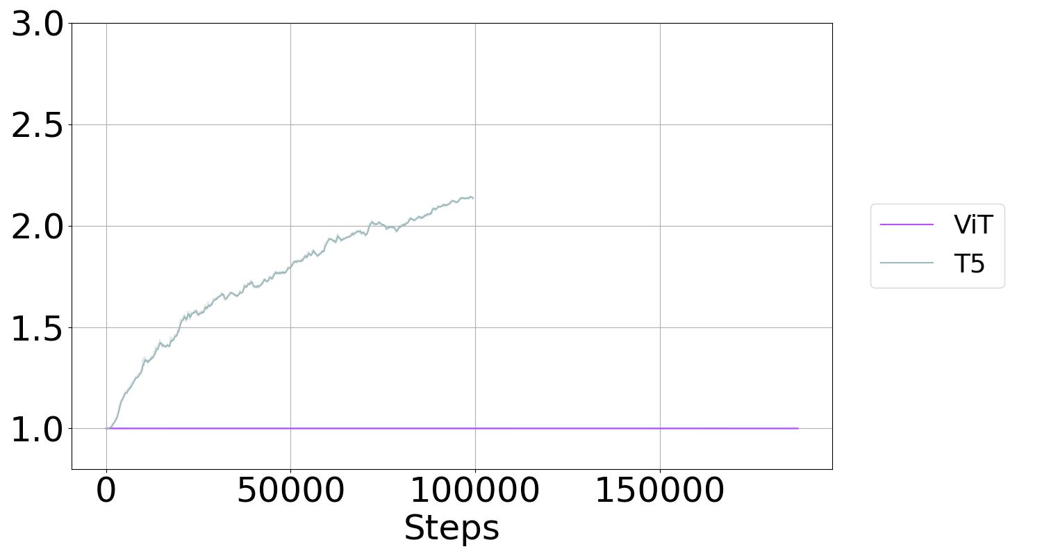


Fig. 12(a) shows an intriguing difference between ViT and T5, i.e., the scaling factors in T5 increase slowly while those in ViT stick to , indicating the latter’s tendency to hold still or to decrease. Whether it is because of architectural or subtle implementation differences or the more interesting differences between CV and NLP tasks remains mysterious. Nevertheless, Fig. 12(a) indicates that the coefficients of gradient sparsity in ViT and T5 is at least and , respectively, most of the time. On the other hand, Fig. 12(b) suggests in ViT, varies a lot across different layers and steps. In shallow layers it can be larger than in the late phase of training, surpassing the coefficients of gradient sparsity. But in deep layers, it is close to , indicating gradient sparsity’s dominance. As a result, for ViT, sparsity in shallow layers and late training relies on direct activation sparsity while that in deep layers is dominated by gradient sparsity. This observation accounts for the gradient sparsity’s weakening in late training as displayed in Fig. 4 because at that time the activation sparsity has enough coefficients to compete with gradient sparsity. In T5, is extremely small, indicating that sparsity is fully due to gradient sparsity instead of direct activation sparsity.
8.4 Spectral Concentration of
The log-scaled histograms of eigenvalues of at several epochs of modified ViT’s entire training on ImageNet-1K are displayed in Fig. 13(a).

 \pgfmathtruncatemacro
1+ı

ıin 0, 50, 100, 150, 200, 250, 299

It can be seen that there is a portion of near-zero () eigenvalues, which are well separated from non-near-zero ones. The portion of near-zero values in Fig. 13(a) is stable and consistent with the theoretical expectation computed by the shape of . For non-near-zero eigenvalues, shallow layers and the last layer tend to have non-concentrating eigenvalues, but all of them still vary within the ratio of and most of them vary within the ratio of , despite that there are about non-near-zero eigenvalues. For deep layers, the majority varies within a ratio of , and the ratio decreases to about during the ending phase of training, indicating a tendency toward concentration as the training proceeds.


ıin 10000, 30000, 50000, 70000, 90000
As displayed in Fig. 14(a), similar phenomena can be observed in the decoder of T5, even though ViT is closer to an encoder. In contrast, the encoder tends to have non-concentrating eigenvalues, demonstrating another interesting difference between encoders and decoders. Nevertheless, the ratio between extreme non-zero eigenvalues in the encoder is not too large during the training. Another difference with ViT is that eigenvalues are much larger in T5, indicating even stronger drives toward (effective) gradient sparsity through the first terms.
8.5 Applicability of Theorem
We measure anisotropy and empirically, as required in Section 4.6. They are compared to hidden dimension or to build empirical evidence for application of Theorem .
Since hidden dimension and weight decay have to be altered, the experiment is conducted on a small data set MNIST(Deng, 2012) and a tiny pure MLP with 1 input layer, 1 classifier layer and hidden linear layers with , each with hidden dimension to be altered. Skip connections and LayerNorm layers are equipped. The models are trained using Cross Entropy Loss and SGD, according to the implicit assumption of Theorem . Inputs of the hidden layers and gradients w.r.t. linear layers’ outputs are collected as vectors and are used to compute , after which s are computed by rescaling. Theorem requires normalization on but it is inefficient to re-normalize after every step. Observing is scaling invariant w.r.t. and essentially captures the expected norm upperbound in in the proof, we directly compute without normalizing and compute the expected norms in , or to illustrate .
in 0.0,0.01,0.1,0.3


LABEL:fig:assumptions_of_spectral_concentration_0.0-LABEL:fig:assumptions_of_spectral_concentration_0.3 show anisotropies, norms and spectral concentration bounds computed by effective window sizes under weight decay of and . From subfigures (a) and (b) in them, significantly drops as increases while increases but never exceeds . Since in bounds Eq. 124 and Eq. 125, is only found within the square root, the increase of has relatively small effects on the bounds. As a result, in subfigures (c)-(f), the estimated bounds decrease as the hidden dimension increases under all experimented weight decay intensities. Among the two bounds, it is theoretically and empirically observed that Eq. 125 based on real parts is more desirable.
As discussed in Section 4.6, weight decay effectively limits and stops bounds’ divergence. From LABEL:fig:assumptions_of_spectral_concentration_0.0 to LABEL:fig:assumptions_of_spectral_concentration_0.3 we can see that as weight decay intensifies, the bounds computed by effective windows size drop significantly, especially in LABEL:fig:assumptions_of_spectral_concentration_0.3 where . Weight decay not only upperbounds , which happens at approximately steps in LABEL:fig:assumptions_of_spectral_concentration_0.3, but also decreases . Note this is not trivial because is scaling invariant. How weight decay causes this drop is worth investigating in future works. When training ViTs, weight decay is usually as large as 0.1 or 0.3 (Dosovitskiy et al., 2020; PyTorch, 2023), so bounds estimated in LABEL:fig:assumptions_of_spectral_concentration_0.1 and LABEL:fig:assumptions_of_spectral_concentration_0.3 suit the practices best, where both and have relatively low spectral ratio bounds smaller than or when hidden dimension is relatively large, which is a low value even though there are hundreds of dimensions.
9 Conclusion
In this work, we explain the activation sparsity observed by Li et al. (2022b) with gradient sparsity and effective gradient sparsity, which emerges from flatness and implicit adversarial robustness. Proofs are done for pure MLPs and other architectures including Transformers under hypothetical massively perturbed training. LayerNorm plays a critical role in them. To argue the effectiveness of zeroth biases, we analyze the phenomenon of spectral concentration in weight matrices by introducing random matrix theory to the research of training dynamics. We propose two sparsity-oriented architectural plug-and-play modifications and one radical modification. Experiments for verification, where our theory predicts well, rule out some potential explanations and provide support for our emphasis on gradient sparsity. We test our modification on ImageNet-1K and C4 to demonstrate its great practical effectiveness. Finetuning for sparsity demonstrates a cheaper way toward better sparsity for existing models. Assumptions made during analyses are empirically validated.
Having demonstrated how sparsity emerges from noises and the robustness against them, we wildly conjecture that a similar explanation applies to sparsity, and thus energy efficiency, in human brains and cognition, which face enormous environmental, sensory and synaptic noises as well as small-batch learning every day and exhibit great robustness against them. Our work also demonstrates that some architectural designs may greatly ease theoretical analyses in deep neural networks, and more theoretically oriented architectures can be proposed in the future. We introduce random matrix theory as a powerful tool in analyzing training dynamics, hoping for its broader application in the machine learning community.
Appendix A Proof of Lemmas
Proof [Proof of Lemma ] Expanding definitions and simple rearrangement give
| (129) |
We first deal with the Hessian within the expectation, i.e., for any there is
| (130) | ||||
| (131) | ||||
| (132) | ||||
| (133) |
Plugging this equality back to Eq. 129 gives
| (134) | ||||
| (135) |
the trace of which is
| (136) | ||||
| (137) | ||||
| (138) | ||||
| (139) | ||||
| (140) |
For well learned model, there is , so given the finiteness of label space there is
| (141) | ||||
| (142) | ||||
| (143) |
where Eq. 143 follows the assumption that outputs a distribution over label space that sums to .
Appendix B More Preliminaries
In this section, we introduce more preliminaries and notations used when proving Theorem .
Recall from Section 3 that for matrices is Schatten norms, or norm conducted on singular values. Additionally, let indicate the spectral norm, i.e. norm or the maximum magnitude of singular values. One major difference with the main text is that complex matrices are involved (although most vectors are still real vectors). So conjugate transposition is substituted for transposition in traces’ connection to Schatten 2-norms and elementwise norms. More properties of traces are involved, for example, Lemma is used to introduce Schatten 1-norm to bound approximation errors.
Lemma 0 (Absolute Trace and Schatten 1-norm)
For real or complex matrix ,
| (144) |
where indicates singular values of and equals to the absolute value of the -th eigenvalue in normal matrices.
Proof This proof is from 23rd (https://math.stackexchange.com/users/46120/23rd). By Schur decomposition, there exists unitary and upper triangular matrix such that . Note that shares the same eigenvalues, which are its diagonal entries, as . There exists such that and . Let and note that is unitary. As a result, there exist unitary matrices and such that
| (145) |
On the other hand, the sum of singular values is also
| (146) |
where is the set of all unitary matrices in . To see this, first notice that the singular value decomposition naturally provides a pair of that achieve . For other unitary matrices, and
| (147) |
Note that is also unitary, whose entries’ magnitudes are no greater than , which implies and Eq. 146 is proved.
With and also unitary, the lemma directly follows.
Schatten 1-norms are usually not direct from assumptions and conditions, so we apply Hölder’s inequality on Schatten norms to produce
| (148) |
where . If is real symmetric positive semi-definite then . If is further an outer product of real vectors, then can be bounded by upperbounds on vector norms. One can also prove
| (149) |
to relate and norms, and thus Schatten 1-norms and 2-norms by seeing them as norms conducted on singular values. The bound on is often provided by Lemma introduced later.
Appendix C Proof of Theorem
More notations and preliminary information are used in the proof. They are listed in Appendix B.
To have a clear goal, we first point out how the ratios in Theorem emerge. In random matrix theory (RMT), a powerful tool is Stieltjes transform when it comes to spectral distribution. Stieltjes transform of a distribution is
| (150) |
where . It can be seen as the expected value of inverses. So if the Stieltjes transform of the spectral distribution’ bound is computed and multiplied with the average eigenvalue that can be computed by trace as the sum of eigenvalues, then the expected fraction is bounded. Lemma fulfills this intuition.
Lemma 0 (Stieltjes transform and eigenvalue ratio)
For any density over real numbers that is only supported on positive numbers, there is
| (151) | ||||
| (152) |
where . As a result, if upperbound or mean of is obtained, one can estimate the averaged ratio between eigenvalues.
Proof By definition,
| (153) | ||||
| (154) | ||||
| (155) |
By setting , there is
| (156) |
We adapt the proof of Theorem 2.1 from Yaskov (2016), where a quadratic equation bridges the Stieltjes transform of the spectral distribution and value . We follow a similar path, but in a non-asymptotic and dependent scenario where it is hard to obtain an residual. So we turn to a generalized form where the residual term is bounded. Lemma explores how we can bound , which is scaled Stieltjes transform of the empirical spectral distribution, by and the magnitude of the residual term.
Lemma 0 (Bounds on continuous roots of a equation)
Suppose is a function of such that
| (157) |
where , and is also a function of . Assume is continuous w.r.t. and further assume always has a non-negative real part. Assume is upperbounded by function where is constant w.r.t. . If for some , there is
| (158) |
then for all , there is
| (159) |
Proof Assume is fixed and .
First of all, since , where is continuous w.r.t. , when well defined is also continuous w.r.t. . Since is well defined for all and has a non-negative real part, meaning , is defined and continuous for all .
implies
| (160) |
where . Consider a modified version of this quadratic equation by altering the zeroth order term
| (161) |
where is a solution of the modified equation. Since depend on in a continuous manner and there is no singular point given , there exist two continuous solutions and to the equation that is well defined for all and where . Conversely, all possible solutions are contained in the union of manifolds given by and . Since
| (162) | ||||
| (163) | ||||
| (164) | ||||
| (165) | ||||
| (166) | ||||
| (167) | ||||
| (168) |
and has no intersection when . As a result, continuous , as for some , can only be found in exactly one of and and thus is either or .
Consider s’ behaviours when . and are either or . By their being continuous and disjoint, and can only be universally one of them otherwise there would be discontinuity. Without loss of generality, let
| (169) | ||||
| (170) |
Assume for contradiction. If so, . Consider the following trajectory of to conclude that :
-
1.
Start from , where .
-
2.
Increase alone until . After this step, term will not flip the sign of given that . Therefore, after this step .
-
3.
Increase alone to . During this step, the term in Eq. 161, which appears under squared root in , changes at most by . Therefore, it will not flip the sign and .
-
4.
Increase to infinity. The influences of and will further drop and become ignorable. So in later parts of the trajectory.
Note since monotonically decreases as increases, step (3) will happen when and the limit following this trajectory is equal to . Therefore, , and . As a result, can be approximated from at .
To this end, taking differentiation (the derivative w.r.t. exists except for a finite number of points given the elementary dependence on it) gives
| (171) |
or
| (172) |
Starting from , there is
| (173) | ||||
| (174) | ||||
| (175) |
where the second inequality follows the triangle inequality for subtracting edges. The third inequality is done by moving towards zero until it is symmetric, during which the end with the largest absolute value is moved to the other end and its absolute value is decreased, enlarging the inverted square root.
As a result, if the residual term is bounded, so are the Stieltjes transform and the expected fraction. In the proof of Yaskov (2016) this quadratic equation is extracted by convergence, which is hard in non-asymptotic analysis. We extract it with approximation, whose error is bounded by vector norm bound , anisotropy bound .
Some matrices are also involved in the approximation, where a technical lemma by Yaskov (2016) is very useful. Lemma states that a special matrix, which we will encounter many times in the following proof, has a bounded spectral norm. Combined with Hölder’s inequality, bounds on matrices’ spectral norms and vector norms () will suppress the approximation error.
Lemma 0 (Lemma 3.1 by Yaskov (2016))
Let be a real symmetric positive semi-definite matrix and . If is such that , then
-
1.
;
-
2.
;
-
3.
;
-
4.
and ;
-
5.
.
With these three lemmas, we can begin the proof of Theorem . Following Yaskov (2016), we relate Stieltjes transform of the spectral distribution with the quadratic equation. The quadratic equation is formed by approximation, whose error becomes in Lemma . After concluding the bounds of the Stieltjes transform, applying Lemma gives the final conclusion.
Proof [Proof of Theorem ]
The proof is adapted from Yaskov (2016) where independence conditions are replaced with Batch Dependence model and new regularities.
Cauchy-Stieltjes transform method is used. When applied to empirical spectral density, by definition there is
| (176) |
for positive semi-definite . Specifically, ’s Stieltjes transform is
| (177) |
To ease presentation, we define to indicate (complex) functions whose magnitudes are bounded by positive real function , i.e.,
| (178) |
where indicates variables other than that relies. will be used combined with “” imitating . Since does not hide constant scaling factors and biases in it, unlike it can be freely added, averaged, multiplied and divided, i.e.,
| (179) | ||||
| (180) |
Consistent with final conclusion, fix () such that throughout the proof. Define . Sample an auxiliary vector so that it is sampled from the conditional distribution given the first batches but it is conditionally independent with other samples in , i.e., an extra sample for the last batch. This dependence relation can be expressed by only adding edges to the SCMs of the Batch Dependence Model. With the auxiliary vector, define .
By Lemma (1), is non-degenerate and
| (181) | ||||
| (182) |
Taking expectations and using the exchangeability within each batch give
| (183) |
Define and note that .
By Lemma (2), there is
| (184) |
We now prove
| (185) |
where is bounded by a function of .
A complex function emerges many times. We will approximate it to the first order so its complex derivative should be computed and bounded.
| (186) |
Therefore, if both stay away from , then on the line connecting and we can approximate by , where . In latter application, , both the start and the end of approximation, is often of form possibly with averaging or expectation missing, where is real symmetric positive semi-definite and is a real vector. The eigenvalues in are
| (187) |
whose real part is
| (188) |
As a result, the real part of inner products is always non-negative and stays away from , and the magnitude of derivatives is .
Another approximation is done between and , whose difference is the outer products of a constant number of random vectors, and it should be minor considering there are of them. Formally, for real symmetric positive semi-definite with eigenvalue decomposition by real matrices and , can be decomposed to , and non-degenerate to where . Let to have . After that, there is
| (189) | ||||
| (190) | ||||
| (191) | ||||
| (192) |
where , the second step is from Sherman-Morrison formula, and the second last inequality is due to Lemma . The fact, that is positive semi-definite whose largest eigenvalue is smaller than the upperbound of ’s eigenvalue magnitude, is also used. To bound the fraction between and , recall the eigenvalue decomposition on
| (193) |
and . Then
| (194) |
where is a real vector. Notice that where both real and imaginary parts are non-negative, and that . With this, the inner products are simplified to
| (195) |
Representing complex numbers by 2-dimensional vectors , there are
| (196) |
Noting that all entries of ’s are non-negative, there is
| (197) |
So . Given that the real part of is non-negative, adding will only increase its magnitude. As a result, there is
| (198) |
When is substituted, there is
| (199) |
In later use, is instantiated by and there is for any , so by assumption the approximation error is always bounded by
| (200) |
With these two approximation techniques, we first approximate the LHS of Eq. 185. To this end, let and by Sherman-Morrison formula there is
| (201) | ||||
| (202) | ||||
| (203) |
After that, there is
| (204) | ||||
| (205) | ||||
| (206) | ||||
| (207) | ||||
| (208) | ||||
| (209) | ||||
| (210) | ||||
| (211) | ||||
| (212) |
where in the last line is a uniformly randomly selected index from independently to the training process.
Note that . So for the term in Eq. 210 we proceed by proving approximates . For convenience let be an alias to it, whose spectral norm satisfies , then
| (213) | ||||
| (214) | ||||
| (215) | ||||
| (216) | ||||
| (217) | ||||
| (218) |
where the last inequality is because
| (219) | ||||
| (220) | ||||
| (221) |
given that is symmetric so that its singular values are absolute eigenvalues. With approximation on complex function , this -boundedness implies approximation of in Eq. 210.
For the difference term in Eq. 211, we prove its diminishment by -bounded variance of , or formally
| (222) | ||||
| (223) |
and
| (224) | ||||
| (225) | ||||
| (226) |
where the last step follows that ’s norm is bounded and that is also uniformly bounded.
To sum up, we have obtained
| (227) |
where .
always have a non-negative real part because real parts of eigenvalues of are always non-negative by an argument similar to previous ones. Since and depend only on instead of , is bounded by which satisfies is constant w.r.t , and . Given , by Lemma , there is
| (230) | ||||
| (231) |
for . Bounds using the real part are similarly obtained.
The similar bound for is
| (232) |
The expected mean of ’s non-zero eigenvalue is
| (233) |
Finally, the desired conclusion is obtained through Lemma by
| (234) |
Appendix D Effective Window Size
We argue that the effective window size should be considered by instead of to have better results, where is learning rate and is the strength of weight decay. The argument relies on another formulation of eigenvalues: corresponds to critical points of Rayleigh quotient
| (235) |
Particularly for weight decayed sample covariances where , its eigenvalues are given by critical points of
| (236) |
So terms are weighted by instead of . Now consider the situation where effective window is used to produce , whose eigenvalues are given by
| (237) |
and consider its difference from those of all samples.
For the smallest non-zero eigenvalues, there is since adding a real symmetric positive semi-definite matrix to to obtain increases all eigenvalues. So we will not be overoptimistic in the smallest non-zero eigenvalues when it comes to bounding the fraction between the largest and smallest non-zero eigenvalues.
For the largest eigenvalues, there is . To see this, let be the unit vector that achieves .
| (238) | ||||
| (239) |
So at most will be overoptimistic by .
As a result, if the exponential weight sum of the out-of-window tail, controlled by instead of , is small, then the over-optimism will be suppressed.
Appendix E Experimental Details
In experiments for validation (Section 6), ViT-Base/16 is trained on CIFAR-10 using Adam. Hyperparameters include learning rate of , batch size of , no dropout, weight decay, learning rate decay or gradient clipping. Random cropping and random horizontal flipping is used as data augmentation. The training lasts for 100 epochs with the first 5 epochs of linear warmup. Automatic mixed precision (AMP) is not used. Note that only and unrefined are used. is not restricted and there are no restricted LayerNorm layers as well. The ViT implementation is based on that of Torch Vision. Logging happens every 10 steps.
During training ViT-Base/16 from scratch on ImageNet-1K, the recipe is adapted from PyTorch (2023). Specifically, the optimizer is AdamW with learning rate , , weight decay , dropout and gradient clipping of global norm . Model EMA is removed to ease experiment tracking. Learning rate is scheduled with cosine annealing without warmup. Batch size is , distributed on 4 GPUs for 300 epochs. Other tricks include mixup of alpha , cutmix of alpha , auto augmentation of policy ra, label smoothing of . AMP with fp16 is used to accelerate training. Images are resized to to save storage. Logging happens every 100 steps. During finetuning, the differences include modifications for sparsity described in Section 5 and Section 7, LoRA of rank , and epoch number reduced to , among which LayerNorm uplifting takes epochs.
During training T5-Base from scratch on C4, the recipe is adapted from Huggingface (2023) and Li et al. (2022b). Specifically, the optimizer is AdamW with learning rate , , weight decay , dropout and gradient clipping of global norm . Learning rate is scheduled with inverse square root scheduling with linear warmup of steps, while the full training lasts for steps. Batch size is . To avoid downloading the entire data set, we use the streaming functionality of Huggingface datasets to download the first training samples without shuffling and the full validation split. Recipe from Huggingface (2023) includes data preparation that concatenates all raw sentences and re-splits them into samples. This step consumes too much storage so we confine the concatenation within a batch and empties are filled with padding tokens that are ignored during computing the loss. This compromise reduces the number of usable samples during training, but there are still approximately at least non-empty samples for every 64 samples. The generation of spans is left unchanged, where 15% of the input is corrupted without any mixture. The encoder receives tokens while tokens are used on the decoder side. Logging happens every 25 steps. When training modified T5, the rented GPUs expired at step . Nevertheless, the effectiveness of modification is already obvious at that step. During finetuning, LoRA of rank and modifications described in Section 5 and Section 7 are equipped. The training step reduces to , among which learning rate warmup takes steps and LayerNorm uplifting and activation function mixing last for steps. Logging happens every steps during finetuning T5.
For experiments in Section 8.5, the tiny MLPs have an input layer of with , five hidden layers of width (or equivalently four hidden linear layers whose matrices are of size ) and one output layer of width . Skip connection is placed across each of the 4 hidden linear layers. LayerNorm layers with affine parameters turned off are also placed before hidden layers. The optimizer is SGD with learning rate . Weight decay is altered as a part of the experiment. Batch size is , the number of epochs is . No learning rate warmup is used because it alters the weight decay after multiplying learning rate during training and bothers the computation of . Data augmentation includes random cropping and random rotation of at most 30 degrees. Logging happens every 20 steps.
Appendix F Theoretically Guided Magic: Massive Perturbation with Small Computation Cost and Good Parallelism
Lemma and Theorem state that by adding massive synaptic noises (non-massive synaptic noises for single tokens can be found in works of Murray and Edwards (1994, 1993)) to weight matrices during forward propagation as in Eq. 77, we are training a times larger effective model and optimizing its flatness w.r.t. these times parameters, where is the number of tokens. These noises can potentially greatly improve the generalization of deep CNNs, Transformers, MLP-Mixers or other architectures as long as they split input into multiple tokens.
However, Eq. 77 requires adding noises to weight matrices independently for each token before matrix multiplication, which is unfriendly to GPUs who prefer stacked matrix multiplication. Direct application of Eq. 77 also requires independent Gaussian noises. Therefore, here we propose an algorithm called that is friendly to parallelism and only requires independent noises, which is the same number as dropout.
The core motivation of is to add noises after matrix multiplication, which is possible by merging multiple Gaussian noises into one. Let be the result of multiplication with s in Eq. 77 and be the -th (column) hidden vector/token in it. Then there is
| (240) | ||||
| (241) |
The summation is a linear combination of independent Gaussian variables, which is also Gaussian. Since entries in are assumed to follow , there is
| (242) |
Note that is only used once for each , so the linear combinations are independent and the perturbed matrix product simplifies to
| (243) |
where -variate Gaussian noise . Therefore, we only need to compute the norm of input tokens, then sample Gaussian noises columnly scaled by them and add the scaled noises to the matrix product, which is . If zeroth biases are removed and LayerNorm layers are placed before linear layers, the squared norm further simplifies to constant .
Interestingly, is theoretically ensured by Lemma and Theorem to encourage flatness if the empirical loss is small enough, even though it is only a first-order optimization and requires only one forward and one backward propagations. Moreover, by using , one is magically expanding the number of parameters. Although their values are correlated, their flatness w.r.t. non-correlated perturbations is indeed optimized. To give a sense of this magical parameter expansion, for ViT-Base, -ed ViT-Base is effectively 197 times larger, with approximately 17B flatness-effective parameters. In NLP tasks this expansion is even larger given the larger number of tokens. can be easily implemented as a PyTorch forward Hook that is registered on all linear layers, which is useful in almost any architectures. For CNN, which can be seen as MLPs with parameters de-duplicated, the computation of input norms can be tricky but is also possible and efficient by all-1-kernel convolution on squared input feature maps.
is a hyperparameter that must be determined beforehand. The noise should be small compared to the magnitudes of entries in weight matrices to allow approximation. However, the norm of parameters may change drastically during training, especially under weight decay. So a more practical solution is to adjust dynamically. We consider a simple solution: for each weight matrix, we compute the average norm of entries in that matrix and multiply it with a pre-determined to obtain . We call it .
The experiments of is under preparation and will come in future works. We introduce it here only for completeness.
References
- 23rd (https://math.stackexchange.com/users/46120/23rd) 23rd (https://math.stackexchange.com/users/46120/23rd). Sum of eigenvalues and singular values. Mathematics Stack Exchange. URL https://math.stackexchange.com/q/386872. URL:https://math.stackexchange.com/q/386872 (version: 2013-05-09).
- Achille and Soatto (2018) Alessandro Achille and Stefano Soatto. Emergence of invariance and disentanglement in deep representations. In 2018 Information Theory and Applications Workshop (ITA), pages 1–9. IEEE, 02 2018. ISBN 978-1-72810-124-8. doi: 10.1109/ITA.2018.8503149. URL https://ieeexplore.ieee.org/document/8503149/.
- Achille et al. (2020) Alessandro Achille, Giovanni Paolini, and Stefano Soatto. Where is the information in a deep neural network?, 06 2020. URL http://arxiv.org/abs/1905.12213.
- Andriushchenko et al. (2023a) Maksym Andriushchenko, Dara Bahri, Hossein Mobahi, and Nicolas Flammarion. Sharpness-aware minimization leads to low-rank features, 05 2023a. URL http://arxiv.org/abs/2305.16292.
- Andriushchenko et al. (2023b) Maksym Andriushchenko, Aditya Vardhan Varre, Loucas Pillaud-Vivien, and Nicolas Flammarion. SGD with large step sizes learns sparse features. In Proceedings of the 40th International Conference on Machine Learning, pages 903–925. PMLR, 07 2023b. URL https://proceedings.mlr.press/v202/andriushchenko23b.html. ISSN: 2640-3498.
- Bricken et al. (2023) Trenton Bricken, Rylan Schaeffer, Bruno Olshausen, and Gabriel Kreiman. Emergence of sparse representations from noise. PMLR, 06 2023. URL https://openreview.net/forum?id=cxYaBAXVKg.
- Bryson et al. (2021) Jennifer Bryson, Roman Vershynin, and Hongkai Zhao. Marchenko-pastur law with relaxed independence conditions, 02 2021. URL http://arxiv.org/abs/1912.12724.
- Chaudhari and Soatto (2018) Pratik Chaudhari and Stefano Soatto. Stochastic gradient descent performs variational inference, converges to limit cycles for deep networks. In 2018 Information Theory and Applications Workshop (ITA), pages 1–10, 02 2018. doi: 10.1109/ITA.2018.8503224.
- Chen et al. (2023) Feng Chen, Daniel Kunin, Atsushi Yamamura, and Surya Ganguli. Stochastic collapse: How gradient noise attracts SGD dynamics towards simpler subnetworks, 06 2023. URL http://arxiv.org/abs/2306.04251.
- Correia et al. (2019) Gonçalo M. Correia, Vlad Niculae, and André F. T. Martins. Adaptively sparse transformers. In Proceedings of the 2019 Conference on Empirical Methods in Natural Language Processing and the 9th International Joint Conference on Natural Language Processing (EMNLP-IJCNLP), pages 2174–2184. Association for Computational Linguistics, 11 2019. doi: 10.18653/v1/D19-1223. URL https://aclanthology.org/D19-1223.
- Dai et al. (2022) Damai Dai, Li Dong, Yaru Hao, Zhifang Sui, Baobao Chang, and Furu Wei. Knowledge neurons in pretrained transformers. In Proceedings of the 60th Annual Meeting of the Association for Computational Linguistics (Volume 1: Long Papers), pages 8493–8502. Association for Computational Linguistics, 2022. doi: 10.18653/v1/2022.acl-long.581. URL https://aclanthology.org/2022.acl-long.581.
- Deng et al. (2009) Jia Deng, Wei Dong, Richard Socher, Li-Jia Li, Kai Li, and Li Fei-Fei. Imagenet: A large-scale hierarchical image database. In 2009 IEEE Conference on Computer Vision and Pattern Recognition, pages 248–255, 2009. doi: 10.1109/CVPR.2009.5206848.
- Deng (2012) Li Deng. The mnist database of handwritten digit images for machine learning research. IEEE Signal Processing Magazine, 29(6):141–142, 2012.
- Dosovitskiy et al. (2020) Alexey Dosovitskiy, Lucas Beyer, Alexander Kolesnikov, Dirk Weissenborn, Xiaohua Zhai, Thomas Unterthiner, Mostafa Dehghani, Matthias Minderer, Georg Heigold, Sylvain Gelly, et al. An image is worth 16x16 words: Transformers for image recognition at scale. In International Conference on Learning Representations, 2020.
- Fedus et al. (2022) William Fedus, Barret Zoph, and Noam Shazeer. Switch transformers: Scaling to trillion parameter models with simple and efficient sparsity. The Journal of Machine Learning Research, 23(1):5232–5270, 2022.
- Georgiadis (2019) Georgios Georgiadis. Accelerating convolutional neural networks via activation map compression. In Proceedings of the IEEE/CVF Conference on Computer Vision and Pattern Recognition, pages 7085–7095, 2019.
- Geva et al. (2021) Mor Geva, Roei Schuster, Jonathan Berant, and Omer Levy. Transformer feed-forward layers are key-value memories. In Proceedings of the 2021 Conference on Empirical Methods in Natural Language Processing, pages 5484–5495. Association for Computational Linguistics, 2021. doi: 10.18653/v1/2021.emnlp-main.446. URL https://aclanthology.org/2021.emnlp-main.446.
- Gotze and Tikhomirov (2006) F. Gotze and A. Tikhomirov. Limit theorems for spectra of positive random matrices under dependence. 133(3):1257–1276, 03 2006. ISSN 1072-3374, 1573-8795. doi: 10.1007/s10958-006-0035-8. URL http://link.springer.com/10.1007/s10958-006-0035-8.
- Götze and Tikhomirov (2004) Friedrich Götze and Alexander Tikhomirov. Rate of convergence in probability to the marchenko-pastur law. Bernoulli, 10(3):503–548, 2004.
- Hoyer (2004) Patrik O Hoyer. Non-negative matrix factorization with sparseness constraints. Journal of machine learning research, 5(9), 2004.
- Huggingface (2023) Huggingface. T5-like span-masked language modeling, 2023. URL https://github.com/huggingface/transformers/tree/main/examples/flax/language-modeling.
- Kaplan et al. (2020) Jared Kaplan, Sam McCandlish, Tom Henighan, Tom B. Brown, Benjamin Chess, Rewon Child, Scott Gray, Alec Radford, Jeffrey Wu, and Dario Amodei. Scaling laws for neural language models, 01 2020. URL http://arxiv.org/abs/2001.08361.
- Keskar et al. (2016) Nitish Shirish Keskar, Dheevatsa Mudigere, Jorge Nocedal, Mikhail Smelyanskiy, and Ping Tak Peter Tang. On large-batch training for deep learning: Generalization gap and sharp minima. In International Conference on Learning Representations, 2016.
- Krizhevsky et al. (2009) Alex Krizhevsky, Geoffrey Hinton, et al. Learning multiple layers of features from tiny images. 2009.
- Kurtz et al. (2020) Mark Kurtz, Justin Kopinsky, Rati Gelashvili, Alexander Matveev, John Carr, Michael Goin, William Leiserson, Sage Moore, Nir Shavit, and Dan Alistarh. Inducing and exploiting activation sparsity for fast inference on deep neural networks. In Proceedings of the 37th International Conference on Machine Learning, pages 5533–5543. PMLR, 11 2020. URL https://proceedings.mlr.press/v119/kurtz20a.html. ISSN: 2640-3498.
- Li et al. (2022a) Bo Li, Yifei Shen, Jingkang Yang, Yezhen Wang, Jiawei Ren, Tong Che, Jun Zhang, and Ziwei Liu. Sparse mixture-of-experts are domain generalizable learners. In The Eleventh International Conference on Learning Representations, 2022a.
- Li et al. (2022b) Zonglin Li, Chong You, Srinadh Bhojanapalli, Daliang Li, Ankit Singh Rawat, Sashank J. Reddi, Ke Ye, Felix Chern, Felix Yu, Ruiqi Guo, and Sanjiv Kumar. The lazy neuron phenomenon: On emergence of activation sparsity in transformers. 09 2022b. URL https://openreview.net/forum?id=TJ2nxciYCk-.
- Lin et al. (2022) Kevin Lin, Linjie Li, Chung-Ching Lin, Faisal Ahmed, Zhe Gan, Zicheng Liu, Yumao Lu, and Lijuan Wang. SwinBERT: End-to-end transformers with sparse attention for video captioning. pages 17949–17958, 2022. URL https://openaccess.thecvf.com/content/CVPR2022/html/Lin_SwinBERT_End-to-End_Transformers_With_Sparse_Attention_for_Video_Captioning_CVPR_2022_paper.html.
- Liu et al. (2015) Haoyang Liu, Alexander Aue, and Debashis Paul. On the marčenko-pastur law for linear time series. 43(2), 04 2015. ISSN 0090-5364. doi: 10.1214/14-AOS1294. URL http://arxiv.org/abs/1310.7270.
- Liu and Wang (2023) Shiwei Liu and Zhangyang Wang. Ten lessons we have learned in the new “sparseland”: A short handbook for sparse neural network researchers, 06 2023. URL http://arxiv.org/abs/2302.02596.
- Liu et al. (2022) Songhua Liu, Jingwen Ye, Sucheng Ren, and Xinchao Wang. DynaST: Dynamic sparse transformer for exemplar-guided image generation. In Shai Avidan, Gabriel Brostow, Moustapha Cissé, Giovanni Maria Farinella, and Tal Hassner, editors, Computer Vision – ECCV 2022, Lecture Notes in Computer Science, pages 72–90. Springer Nature Switzerland, 2022. ISBN 978-3-031-19787-1. doi: 10.1007/978-3-031-19787-1˙5.
- Marčenko and Pastur (1967) V A Marčenko and L A Pastur. DISTRIBUTION OF EIGENVALUES FOR SOME SETS OF RANDOM MATRICES. 1(4):457–483, 04 1967. ISSN 0025-5734. doi: 10.1070/SM1967v001n04ABEH001994. URL https://iopscience.iop.org/article/10.1070/SM1967v001n04ABEH001994.
- Merrill et al. (2021) William Merrill, Vivek Ramanujan, Yoav Goldberg, Roy Schwartz, and Noah A. Smith. Effects of parameter norm growth during transformer training: Inductive bias from gradient descent. In Proceedings of the 2021 Conference on Empirical Methods in Natural Language Processing, pages 1766–1781. Association for Computational Linguistics, 11 2021. doi: 10.18653/v1/2021.emnlp-main.133. URL https://aclanthology.org/2021.emnlp-main.133.
- Murray and Edwards (1993) Alan F Murray and Peter J Edwards. Synaptic weight noise during multilayer perceptron training: fault tolerance and training improvements. IEEE Transactions on Neural Networks, 4(4):722–725, 1993.
- Murray and Edwards (1994) Alan F Murray and Peter J Edwards. Enhanced mlp performance and fault tolerance resulting from synaptic weight noise during training. IEEE Transactions on neural networks, 5(5):792–802, 1994.
- Orvieto et al. (2022) Antonio Orvieto, Hans Kersting, Frank Proske, Francis Bach, and Aurelien Lucchi. Anticorrelated noise injection for improved generalization. In Proceedings of the 39th International Conference on Machine Learning, pages 17094–17116. PMLR, 06 2022. URL https://proceedings.mlr.press/v162/orvieto22a.html. ISSN: 2640-3498.
- Puigcerver et al. (2022) Joan Puigcerver, Rodolphe Jenatton, Carlos Riquelme, Pranjal Awasthi, and Srinadh Bhojanapalli. On the adversarial robustness of mixture of experts. In S. Koyejo, S. Mohamed, A. Agarwal, D. Belgrave, K. Cho, and A. Oh, editors, Advances in Neural Information Processing Systems, volume 35, pages 9660–9671. Curran Associates, Inc., 2022. URL https://proceedings.neurips.cc/paper_files/paper/2022/file/3effb91593c4fb42b1da1528328eff49-Paper-Conference.pdf.
- PyTorch (2023) PyTorch. vision/references/classification at main · pytorch/vision, 2023. URL https://github.com/pytorch/vision/tree/main/references/classification.
- Raffel et al. (2020) Colin Raffel, Noam Shazeer, Adam Roberts, Katherine Lee, Sharan Narang, Michael Matena, Yanqi Zhou, Wei Li, and Peter J. Liu. Exploring the limits of transfer learning with a unified text-to-text transformer. Journal of Machine Learning Research, 21(140):1–67, 2020. URL http://jmlr.org/papers/v21/20-074.html.
- Ren et al. (2023) Qihan Ren, Jiayang Gao, Wen Shen, and Quanshi Zhang. Where we have arrived in proving the emergence of sparse symbolic concepts in AI models, 05 2023. URL http://arxiv.org/abs/2305.01939.
- Riquelme et al. (2021) Carlos Riquelme, Joan Puigcerver, Basil Mustafa, Maxim Neumann, Rodolphe Jenatton, André Susano Pinto, Daniel Keysers, and Neil Houlsby. Scaling vision with sparse mixture of experts. In Advances in Neural Information Processing Systems, volume 34, pages 8583–8595. Curran Associates, Inc., 2021. URL https://proceedings.neurips.cc/paper/2021/hash/48237d9f2dea8c74c2a72126cf63d933-Abstract.html.
- Sagun et al. (2018) Levent Sagun, Utku Evci, V. Ugur Guney, Yann Dauphin, and Leon Bottou. Empirical analysis of the hessian of over-parametrized neural networks. 2018. URL https://openreview.net/forum?id=rJO1_M0Lf.
- Simsekli et al. (2019) Umut Simsekli, Levent Sagun, and Mert Gurbuzbalaban. A tail-index analysis of stochastic gradient noise in deep neural networks. In Proceedings of the 36th International Conference on Machine Learning, pages 5827–5837. PMLR, 05 2019. URL https://proceedings.mlr.press/v97/simsekli19a.html. ISSN: 2640-3498.
- (44) David So, Wojciech Mańke, Hanxiao Liu, Zihang Dai, Noam Shazeer, and Quoc V Le. Searching for efficient transformers for language modeling. In Advances in Neural Information Processing Systems, volume 34, pages 6010–6022. Curran Associates, Inc. URL https://proceedings.neurips.cc/paper_files/paper/2021/hash/2f3c6a4cd8af177f6456e7e51a916ff3-Abstract.html.
- Stutz et al. (2021) David Stutz, Matthias Hein, and Bernt Schiele. Relating adversarially robust generalization to flat minima. In Proceedings of the IEEE/CVF International Conference on Computer Vision, pages 7807–7817, 2021. URL https://openaccess.thecvf.com/content/ICCV2021/html/Stutz_Relating_Adversarially_Robust_Generalization_to_Flat_Minima_ICCV_2021_paper.html.
- Tolstikhin et al. (2021) Ilya O Tolstikhin, Neil Houlsby, Alexander Kolesnikov, Lucas Beyer, Xiaohua Zhai, Thomas Unterthiner, Jessica Yung, Andreas Steiner, Daniel Keysers, Jakob Uszkoreit, et al. Mlp-mixer: An all-mlp architecture for vision. Advances in neural information processing systems, 34:24261–24272, 2021.
- Yao (2012) Jianfeng Yao. A note on a marčenko–pastur type theorem for time series. Statistics & probability letters, 82(1):22–28, 2012.
- Yaskov (2016) Pavel Yaskov. A short proof of the marchenko–pastur theorem. Comptes Rendus Mathematique, 354(3):319–322, 2016.
- Zhang et al. (2018) Guodong Zhang, Chaoqi Wang, Bowen Xu, and Roger Grosse. Three mechanisms of weight decay regularization. In International Conference on Learning Representations, 2018.
- Zhou et al. (2020) Pan Zhou, Jiashi Feng, Chao Ma, Caiming Xiong, Steven Chu Hong Hoi, and Weinan E. Towards theoretically understanding why sgd generalizes better than adam in deep learning. In Advances in Neural Information Processing Systems, volume 33, pages 21285–21296. Curran Associates, Inc., 2020. URL https://proceedings.neurips.cc/paper/2020/hash/f3f27a324736617f20abbf2ffd806f6d-Abstract.html.