Mass density vs. energy density
at cosmological scales

Abstract

In the presence of the gravitational field, the energy density of matter no longer coincides with its mass density. A discrepancy exists, of course, also between the associated power spectra. Within the $\Lambda$CDM model, we derive a formula that relates the power spectrum of the energy density to that of the mass density and test it with the help of N-body simulations run in comoving boxes of 2.816 Gpc/$h$. The results confirm the validity of the derived formula and simultaneously show that the power spectra diverge significantly from one another at large cosmological scales.

1 Introduction

Upcoming galaxy surveys such as [1, 2] are expected to probe the distribution of large-scale inhomogeneities at unprecedented scales and with remarkable precision. However, in order to study the large-scale structure at gigaparsec scales, one still needs to resort to N-body simulations. In doing so, it must be taken into account that relativistic effects play an important role in such large domains and hence, the corresponding numerical code should be solving the complete system of general relativistic field equations.

Recently, the all-scale cosmological perturbation theory has been formulated in a relativistic approach, which employs linearized field equations [3, 4] that can be solved analytically for metric perturbations. It has been shown that the first-order expression for the gravitational potential has a Yukawa-type form, and the gravitational force starts to decay exponentially at scales of 2-3 Gpc [5] unlike what is expected of its Newtonian counterpart. Employing the publicly available relativistic code gevolution [6, 7], this so-called screening of gravity at large cosmological scales has been studied also via N-body simulations in [8], in terms of the behaviour of the power spectrum of the mass density contrast. As expected, it has been revealed that growth of matter overdensities is suppressed beyond the time-dependent characteristic cutoff scale, i.e. the screening length.

In the presence of the gravitational field, the energy density of matter (which corresponds to the mixed 00-component of the energy-momentum tensor) differs from its mass density [9], and it is surely nontrivial to obtain a formula connecting the power spectra of the two quantities. From the point of view of screening formalism, the quantity relevant to matter fluctuations is the mass density contrast [3]. The analytical derivation of such a formula is provided in the present work for the $\Lambda$CDM model. It is then tested via studying the behaviour of the power spectra of both quantities, extracted from N-body simulations carried out in boxes of 2.816 Gpc/$h$ in comoving size.

The paper is structured as follows: in Section 2, we derive a formula that relates the power spectrum of the energy density to that of the mass density in the $\Lambda$CDM model. In Section 3, we verify this formula based on simulation outputs. Results are briefly summarized in concluding Section 4.

2 Relation between the power spectra of energy and mass densities

In the $\Lambda$CDM model, the perturbed Friedmann-Lemaître-Robertson-Walker metric in the conformal Newtonian gauge reads [10, 11]

$$ds^{2}=a^{2}\left[(1+2\Phi)d\eta^{2}-(1-2\Phi)\delta_{ij}dx^{i}dx^{j}\right]\,,\quad i,j=1,2,3\,,$$ (1)

where, within the scope of our research, we consider only first-order scalar perturbations $\Phi$ (with $|\Phi|\ll 1$), representing the gravitational potential. $a(\eta)$ is the scale factor (depending on the conformal time $\eta$) and $x^{i}$ denote the comoving coordinates.

For cold dark matter (CDM), fluctuations of the energy density in the first-order are described as [3, 12]

$$\delta\varepsilon\equiv\varepsilon-\bar{\varepsilon}=\frac{c^{2}}{a^{3}}\delta\rho+\frac{3c^{2}}{a^{3}}\overline{\rho}\Phi\,,$$ (2)

where

$$\delta\rho\equiv\rho-\bar{\rho}$$ (3)

is the comoving mass density fluctuation. The average value of the energy density $\bar{\varepsilon}$ is related to that of the comoving mass density as $\bar{\varepsilon}=\bar{\rho}c^{2}/a^{3}$. On the other hand, from the Friedmann equation we get

$$\bar{\varepsilon}=\frac{1}{\kappa}\left(\frac{3{\mathcal{H}^{2}}}{a^{2}}-\Lambda\right),$$ (4)

where $\mathcal{H}\equiv(da/d\eta)/a$ is the conformal Hubble parameter and $\kappa\equiv 8\pi G_{N}/c^{4}$, with $c$ standing for the speed of light and $G_{N}$ for the Newtonian gravitational constant.

As follows from Eq. (2), for non-vanishing gravitational field (the potential $\Phi$), $\delta\varepsilon$ deviates from the definition of mass density fluctuations, which reads $\delta\rho/a^{3}$. Within the cosmic screening approach, the gravitational potential $\Phi$ satisfies the Helmholtz-type equation [5]

$$\bigtriangleup\Phi-\frac{a^{2}}{\lambda_{\rm{eff}}^{2}}\Phi=\frac{\kappa c^{2}}{2a}\delta\rho\,,$$ (5)

where $\bigtriangleup\equiv\delta^{ij}\partial_{i}\partial_{j}$ (with $\partial_{i}\equiv\partial/\partial x^{i}$) is the Laplace operator, and

$$\lambda_{\rm{eff}}(\eta)=\left(\frac{a\mathcal{H}}{3}\int_{0}^{a}\frac{d\tilde{a}}{\mathcal{H}^{3}}\right)^{1/2}\,$$ (6)

determines the characteristic length of the Yukawa-type cutoff for gravitational interactions. For $\Lambda$CDM cosmology and based on the Planck data reported in [13], its current value is found to be $\lambda_{{\rm{eff}},0}=2.57$ Gpc.

Eq. (2) shows the relationship between fluctuations in the energy density and mass density. Now, in order to formulate the relationship between the power spectra of these quantities, we resort to the definition [6]

$$4\pi k^{3}\langle\widehat{X}({\bf{k}},z)\,\widehat{X}({\bf{k}}^{\prime},z)\rangle=(2\pi)^{3}\delta_{\rm D}({\bf k}-{\bf k}^{\prime})P_{X}(k,z)\,$$ (7)

that applies to some variable $X({\bf{r}},z)$ at redshift $z$, where $\delta_{\rm D}({\bf k}-{\bf k}^{\prime})$ stands for the Dirac delta function. The hat denotes the Fourier transform of the respective quantity. The dimensionless power spectrum $P_{X}(k,z)$ [14] is the Fourier transform

$$P_{X}(k,z)=4\pi k^{3}\int\frac{d^{3}{\bf{r}}}{(2\pi)^{3}}\xi_{X}(r,z)\exp(i{\bf{k}}{\bf{r}})$$ (8)

of the two-point correlation function

$$\xi_{X}(r,z)=\frac{1}{V}\int d{\bf{x}}X({\bf{x}},z)X({\bf{x}}+{\bf{r}},z)\,,$$ (9)

defined in the volume $V$. It is worth noting that an alternative definition of the power spectrum is also often used in the literature, that reads $\tilde{P}_{X}(k,z)=\left(2\pi^{2}/k^{3}\right)P_{X}(k,z)$ [11]. Due to statistical homogeneity and isotropy, $\xi_{X}$ depends on $r\equiv|{\bf{r}|}$, and $P_{X}$ depends on $k\equiv|{\bf{k}}|$ [14]. From this point on we drop the redshift dependence to avoid cluttered notation.

Based on Eq. (2), the correlation function for energy density fluctuations can be written in the form

$$\xi_{\delta\varepsilon}(x) = \frac{1}{V}\int d{\bf{r}}\delta\varepsilon({\bf{r}})\delta\varepsilon({\bf{r}}+{\bf{x}})$$ (10)

$$= \frac{1}{V}\int d{\bf{r}}\left[\frac{c^{2}}{a^{3}}\delta\rho({\bf r})+\frac{3c^{2}}{a^{3}}\overline{\rho}\Phi({\bf r})\right]\left[\frac{c^{2}}{a^{3}}\delta\rho({\bf r}+{\bf x})+\frac{3c^{2}}{a^{3}}\overline{\rho}\Phi({\bf r}+{\bf x})\right]$$

$$= \left(\frac{c^{2}}{a^{3}}\right)^{2}\xi_{\delta\rho}(x)+\left(\frac{3c^{2}}{a^{3}}\overline{\rho}\right)^{2}\xi_{\Phi}(x)\,$$

$$+ 3\overline{\rho}\left(\frac{c^{2}}{a^{3}}\right)^{2}\frac{1}{V}\left[\int d{\bf{r}}\delta\rho({\bf r})\Phi({\bf r}+{\bf x})+\int d{\bf{r}}\Phi({\bf r})\delta\rho({\bf r}+{\bf x})\right]\,.$$

To calculate the integrals in the last row, we note that

$$\bigtriangleup_{\bf x}\xi_{\Phi}(x) = \frac{1}{V}\int d{\bf r}\Phi({\bf r})\bigtriangleup_{\bf x}\Phi({\bf r}+{\bf x})$$ (11)

$$= \frac{1}{V}\int d{\bf r}\Phi({\bf r})\left[\frac{a^{2}}{\lambda_{\rm{eff}}^{2}}\Phi({\bf r}+{\bf x})+\frac{\kappa c^{2}}{2a}\delta\rho({\bf r}+{\bf x})\right]\,,$$

where we make use of use Eq. (5). Consequently, we get

$$\frac{1}{V}\int d{\bf{r}}\Phi({\bf r})\delta\rho({\bf r}+{\bf x})=\left(\frac{\kappa c^{2}}{2a}\right)^{-1}\left[\bigtriangleup_{\bf x}\xi_{\Phi}(x)-\frac{a^{2}}{\lambda_{\rm{eff}}^{2}}\xi_{\Phi}(x)\right]\,.$$ (12)

Meanwhile,

$$\int d{\bf{r}}\Phi({\bf r})\delta\rho({\bf r}+{\bf x})=\int d{\bf{r}}\Phi({\bf r}-{\bf x})\delta\rho({\bf r})=\int d{\bf{r}}\Phi({\bf r}+{\bf x})\delta\rho({\bf r})\,,$$ (13)

where in the last equality, we exploited the invariance of the right-hand side of Eq. (12) with respect to the sign of ${\bf x}$. Since the left-hand side must also be invariant under the same transformation, the correlation function for the energy density fluctuation reads

$$\xi_{\delta\varepsilon}(x)=\frac{c^{4}}{a^{6}}\xi_{\delta\rho}(x)+9{\bar{\varepsilon}}^{2}\xi_{\Phi}(x)+\frac{12}{\kappa}\bar{\varepsilon}\left[\frac{1}{a^{2}}\bigtriangleup_{\bf x}\xi_{\Phi}(x)-\frac{1}{\lambda_{\rm{eff}}^{2}}\xi_{\Phi}(x)\right]\,.$$ (14)

Finally, for the power spectra, we obtain the formula

$$P_{\delta\varepsilon}(k)=\frac{c^{4}}{a^{6}}P_{\delta\rho}(k)+3\bar{\varepsilon}\left[3\bar{\varepsilon}-\frac{4}{\kappa}\left(\frac{k^{2}}{a^{2}}+\frac{1}{\lambda_{\rm{eff}}^{2}}\right)\right]P_{\Phi}(k)\,,$$ (15)

where we have taken into account that the Fourier transform of $\bigtriangleup_{\bf x}\xi_{\Phi}(x)$ gives $-k^{2}P_{\Phi}(k)$.

3 Validation via N-body simulations

In the following step, we test the validity of the formula in Eq. (15) employing N-body simulations. It was shown previously in [15] that the power spectra of scalar (and vector) perturbations agree to high accuracy when simulated according to the screening approach versus the default formulation of the relativistic code $gevolution$, despite the differences in how the weak field expansion is performed within two schemes. That is why, for the current study, we were able to simulate the power spectrum $P_{\delta\varepsilon}$ on the left-hand side (LHS) of Eq. (15) using gevolution [6, 7] without any modifications. The power spectra $P_{\delta\rho}$ and $P_{\Phi}$ on the right-hand side (RHS), however, were obtained in a second run, based on the set of equations of the cosmic screening approach: the $\Phi$-dependent term in the full expression for $\delta\varepsilon=\delta T^{0}_{0}=T^{0}_{0}-\overline{T_{0}^{0}}$ (where the energy-momentum tensor element $T_{0}^{0}$ is given by (3.7) of [7]) was moved to the LHS of the corresponding field equation in gevolution, that is, (2.9) in [7], and the remaining term $\propto\delta\rho$ was left as the single first-order source on the RHS upon removing the extra terms proportional to squared momenta, negligible for nonrelativistic bodies with the comoving mass density $\rho=\sum_{n}m_{n}\delta({\bf r}-{\bf r}_{n})$ in our configuration. All second-order contributions were also removed from the LHS to match the weak field expansion employed in the screening approach (as worked out explicitly in [15]).

Introducing the notations

$$P^{\rm g}_{\delta} \equiv P_{\delta\varepsilon/{\bar{\varepsilon}}}=\frac{1}{\bar{\varepsilon}^{2}}P_{\delta\varepsilon}\,,$$ (16)

$$P^{\rm s}_{\delta} \equiv P_{\delta\rho/{\bar{\rho}}}=\frac{1}{\bar{\rho}^{2}}P_{\delta\rho}\,,$$ (17)

Eq. (15) may be reformulated as

$$P_{\delta}^{\rm g}(k,z)=P_{\delta}^{\rm s}(k,z)+3\left[3-\frac{4}{\kappa{\bar{\varepsilon}}}\left(\frac{k^{2}}{a^{2}}+\frac{1}{\lambda_{\rm{eff}}^{2}}\right)\right]P_{\Phi}(k,z)\,.$$ (18)

To test the above expression, we have run two simulations, both in boxes with comoving sizes of 2816 Mpc/$h$ at 1 Mpc/$h$ resolution, as explained above. For $\Lambda$CDM cosmology, the parameters used were $H_{0}=67.66\,{\rm km}\,{\rm s}^{-1}{\rm Mpc}^{-1}$, $\Omega_{\rm M}h^{2}=\Omega_{\rm b}h^{2}+\Omega_{\rm c}h^{2}=0.14175$, where $h=0.6766$, and $\Omega_{\Lambda}=1-\Omega_{\rm M}$ [13]. Baryons and cold dark matter have been treated on equal footing and the scale factor at the present time was set to $a_{0}=1$.

Four pairs of curves are depicted in Fig. 1 corresponding to redshifts $z=80,50,15$ and $z=0$. In each pair, one curve corresponds to the LHS of Eq. (18) (i.e. $P_{\delta}^{\rm g}$), and the second one to the full expression on the RHS. To estimate the difference between the left- and right-hand sides of (18) quantitatively, we introduce the relative deviation

$$\Delta\equiv\left|\frac{P^{\mathrm{g}}_{\delta}-P^{\mathrm{RHS}}_{\delta}}{P^{\mathrm{g}}_{\delta}}\right|$$ (19)

for each pair. Fig. 2 demonstrates that relative deviations reach their maximum values at small momenta $k$ (i.e. large scales) and large redshifts. Nevertheless, the curves which correspond to the RHS of (18) are within the standard deviation of $P^{\mathrm{g}}_{\delta}$ (see Fig. 3). So large values of $\Delta$ are mostly associated with the inaccuracy of calculations at the larger scales in the simulation, intrinsically represented with relatively less data points in the k-space of the box used.

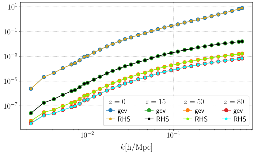
Figure 1: Four pairs of curves corresponding to the left- (gev) and right-hand (RHS) sides of Eq. (18) at redshifts $z=80,50,15$ and $z=0$ from bottom to top.

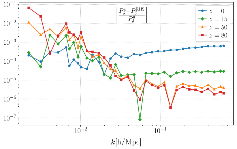
Figure 2: Relative deviations given by Eq. (19) for four pairs of curves in Fig (1).

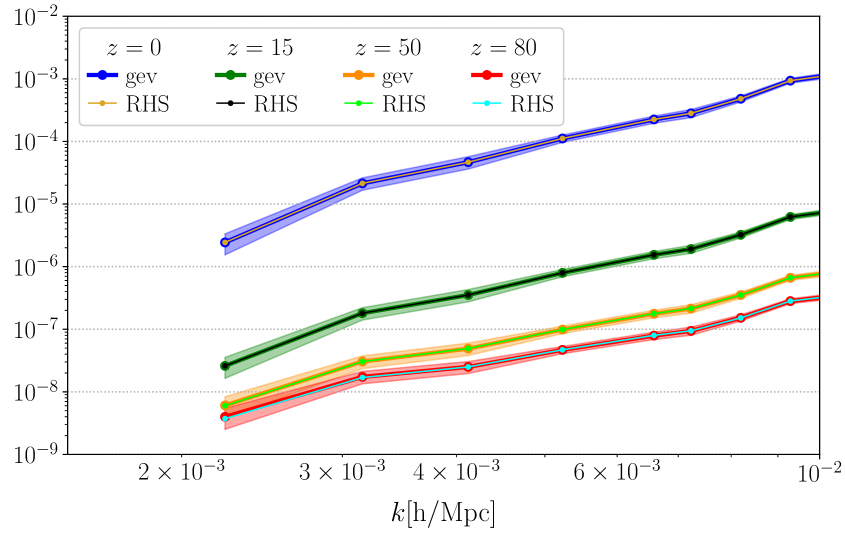
Figure 3: Standard deviations of power spectra $P^{\mathrm{g}}_{\delta}$ (gev) at redshifts $z=80,50,15$ and $z=0$ from bottom to top. All curves that correspond to the RHS of Eq. (18) remain within the respective shaded regions.

It is, of course, of interest to compare the power spectrum of energy density contrast $P^{\mathrm{g}}_{\delta}$ to that of the mass density contrast $P^{\mathrm{s}}_{\delta}$ too. The respective curves are presented in Fig. 4, in which a significant deviation is observed for small momenta and large $z$. This is because, at large cosmological scales, the second term on the RHS of Eq. (18), $\propto P_{\Phi}$, becomes non-negligible with respect to the power spectrum for the mass density contrast $P_{\delta}^{s}$.

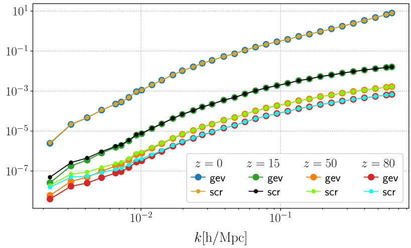
Figure 4: Power spectra of $P^{\mathrm{g}}_{\delta}$ (gev) and $P^{\mathrm{s}}_{\delta}$ (scr) at redshifts $z=80,50,15$ and $z=0$ from bottom to top. This figure demonstrates the significant divergence at small momenta $k$ and large redshifts.

4 Conclusion

In the present paper we have considered the power spectra of energy and mass density fluctuations for the $\Lambda$CDM model. The energy density of matter does not coincide with the mass density in the presence of the gravitational field, and the respective power spectra differ also. In attempt to quantify the discrepancy, we have first derived the analytical expression for the relationship between two power spectra, and then tested it with the help of N-body simulations carried out in boxes of 2.816 Gpc/$h$ comoving sizes. We have calculated the power spectrum of the energy density contrast using gevolution [7]. To calculate the power spectrum of the mass density contrast, we have modified the code to recover the corresponding equations in the cosmic screening approach [8, 15]. Numerical simulations have confirmed that the derived formula works well. We have also shown that the power spectra of the energy density contrast and the mass density contrast diverge significantly at large cosmological scales where relativistic effects are essential.

Data Availability

The datasets generated in this work are publicly available in the Rossendorf Data Repository (RODARE) and may be accessed via the link https://rodare.hzdr.de/record/2469

References

- [1] R. Laureijs et al. [EUCLID collaboration], Euclid Definition Study Report. arXiv:1110.3193 [astro-ph.CO].
- [2] P.A. Abell et al. [LSST Science and LSST Project Collaborations], LSST Science Book, Version 2.0. arXiv:0912.0201 [astro-ph.IM].
- [3] M. Eingorn, First-order cosmological perturbations engendered by point-like masses. Astrophys. J. 825, 84 (2016). arXiv:1509.03835 [gr-qc].
- [4] M. Eingorn, C. Kiefer, A. Zhuk, Scalar and vector perturbations in a universe with discrete and continuous matter sources. JCAP 09, 032 (2016). arXiv:1607.03394 [gr-qc].
- [5] E. Canay, M. Eingorn, Duel of cosmological screening lengths. Phys. Dark Univ. 29, 100565 (2020). arXiv:2002.00437 [gr-qc].
- [6] J. Adamek, D. Daverio, R. Durrer, M. Kunz, General relativity and cosmic structure formation. Nature Phys. 12, 346 (2016). arXiv:1509.01699 [astro-ph.CO].
- [7] J. Adamek, D. Daverio, R. Durrer, M. Kunz, gevolution: a cosmological N-body code based on General Relativity. JCAP 07, 053 (2016). arXiv:1604.06065 [astro-ph.CO].
- [8] M. Eingorn, E. Yilmaz, A.E. Yükselci, A. Zhuk, Suppression of matter density growth at scales exceeding the cosmic screening length. arXiv:2307.06920 [gr-qc].
- [9] L.D. Landau, E.M. Lifshitz, Course of Theoretical Physics Series, Vol. 2, The Classical Theory of Fields. Oxford Pergamon Press, Oxford (2000).
- [10] V.F. Mukhanov, Physical foundations of cosmology. Cambridge University Press, Cambridge (2005).
- [11] D.S. Gorbunov, V.A. Rubakov, Introduction to the Theory of the Early Universe: Cosmological Perturbations and Inflationary Theory. World Scientific, Singapore (2011).
- [12] M. Eingorn, A. Zhuk, Hubble flows and gravitational potentials in observable Universe. JCAP 09, 026 (2012). arXiv:1205.2384 [astro-ph.CO].
- [13] N. Aghanim et al. [Planck Collaboration], Planck 2018 results. VI. Cosmological parameters. Astron. Astrophys. 641, A6 (2020). arXiv:1807.06209 [astro-ph.CO].
- [14] F. Bernardeau, S. Colombi, E. Gaztanaga, R. Scoccimarro, Large-scale structure of the universe and cosmological perturbation theory. Phys. Rept. 367, 1 (2002). arXiv:astro-ph/0112551.
- [15] M. Eingorn, A.E. Yükselci, A. Zhuk, Screening vs. gevolution: in chase of a perfect cosmological simulation code. Phys. Lett. B 826, 136911 (2022). arXiv:2106.07638 [gr-qc].