Fast time-stepping discontinuous Galerkin method for the subdiffusion equation

Abstract. The nonlocality of the fractional operator causes numerical difficulties for long time computation of the time-fractional evolution equations. This paper develops a high-order fast time-stepping discontinuous Galerkin finite element method for the time-fractional diffusion equations, which saves storage and computational time. The optimal error estimate $O(N^{-p-1}+h^{m+1}+\varepsilon N^{r\alpha})$ of the current time-stepping discontinuous Galerkin method is rigorous proved, where $N$ denotes the number of time intervals, $p$ is the degree of polynomial approximation on each time subinterval, $h$ is the maximum space step, $r\geq 1$, $m$ is the order of finite element space, and $\varepsilon>0$ can be arbitrarily small. Numerical simulations verify the theoretical analysis.

Key words. fast time-stepping discontinuous Galerkin method, optimal convergence, subdiffusion, nonlocality.

MSC codes. 26A33, 65M06, 65M12, 65M15, 35R11

1 Introduction

The aim of this paper is to develop the fast time-stepping discontinuous Galerkin (DG) finite element method (FEM) for the following subdiffusion equation

(1) $$\left\{\begin{aligned} &{}_{0}^{C}D_{t}^{\alpha}u(x,t)+\mathcal{L}u(x,t)=f(x,t),&&(x,t)\in\Omega\times(0,T],T>0,\\ &u(x,0)=u_{0}(x),&&x\in\bar{\Omega},\\ &u(x,t)=0,&&(x,t)\in\partial\Omega\times[0,T],\end{aligned}\right.$$

where $x=(x_{1},x_{2},...,x_{d})\in\Omega\subset\mathbb{R}^{d}$ is a bounded Lipschitz domain, $d\in\{1,2,3\}$, $\mathcal{L}$ is a linear second-order elliptic operator, and the Caputo fractional derivative operator ${}_{a}^{C}D_{t}^{\alpha}$ is defined by

(2) $${}_{a}^{C}D_{t}^{\alpha}u(x,t)=\frac{1}{\Gamma(1-\alpha)}\int_{a}^{t}\frac{\partial u(x,s)}{\partial s}(t-s)^{-\alpha}\mathrm{d}s,\quad 0<\alpha<1,\,\,a\in\mathbb{R}.$$

For simplicity of analysis, we consider $\mathcal{L}=-\Delta$ in the paper. The subdiffusion equations, which can model the sublinear growth of mean squared particle displacement in transport processes, have attracted much interests of physicists, engineers and applied mathematicians in developing highly accurate and efficient computational methods and numerical analysis.

The regularity of the solution of (1) has been fully understood in literature [14, 16, 29]. In this paper, we assume that the solution $u(t)=u(\cdot,t)$ of (1) satisfies the following finite regularity:

(3) $$\|u^{(\ell)}(t)\|_{H^{q}(\Omega)}\leq C(1+t^{\sigma-\ell}),\quad t>0,$$

where $C>0$, $\sigma>0$, $0\leq\ell\leq p+1$, $p$ and $q$ are nonnegative integers depending the smoothness of the initial data and the source term $f(x,t)$, and $u^{(\ell)}(t)$ denotes the $\ell$-th order time derivative of $u(t)=u(\cdot,t)$; see [16], in which $\sigma=\alpha$ can be obtained. From (3), one will find that there exists the initial singularity of the solution to (1). We employ the adaptive mesh to deal with the numerical difficulty of the singularity, see, e.g., [30].

The non-locality of the fractional derivative operator (2) causes a lot of numerical difficulty for solving (1), especially for long time computation and high dimension space models. Generally speaking, the approximation of the fractional derivative ${}_{0}^{C}D_{t}^{\alpha}u(t_{n})$ takes the form of (see, e.g., [2, 9, 20])

$$\sum_{j=0}^{n}w_{n,j}u(t_{j}),\quad 1\leq n\leq N,$$

where $w_{n,j}$ depends on specific time discretization methods, the fractional order $\alpha$, and the temporal mesh.

There have been a lot of numerical methods for solving (1), readers can refer to papers [13, 15, 20, 29, 34] and the books of fractional calculus [8, 14, 19, 31]. For the fast memory-saving time-stepping methods, readers can refer to [3, 4, 6, 10, 12, 21, 33], where the fast methods are designed to directly discretize the fractional integral or derivatives. Here, we extend the ideas of the fast methods in the aforementioned papers to calculate the integral arising from the time-stepping DG methods. Time-stepping DG schemes have been developed to solve time-fractional diffusion and diffusion wave equations as $u_{t}(t)+\partial_{t}^{\beta}(\mathcal{L}u)(t)=g(x,t),-1<\beta<1$, readers can refer to [17, 18, 23, 25] for more details.

To the best of our knowledge, the only work of the time-stepping DG method for (1) was developed by Mustapha and his collaborators in [24], where they proposed a linear time-stepping DG method (see (13) with $p=1$). Under the regularity condition $\|u^{\prime}(t)\|_{H^{2}(\Omega)}+t\|u^{\prime\prime}(t)\|_{H^{1}(\Omega)}\leq Ct^{\sigma-1},t>0,C\geq 0$, and $\sigma>\alpha/2$, Mustapha et al. proved the following error bound [24, Theorem 3]

(4) $$\int_{0}^{t_{n}}\|U_{h}(t)-u(t)\|^{2}\textrm{d}t\leq C(N^{-(4-\alpha)}+h^{4}),\quad r\geq\frac{4-\alpha}{2\sigma-\alpha},$$

where $U_{h}(t)$ is the DG solution. In this paper, we obtain the optimal error bound

(5) $$\int_{0}^{t_{n}}\|U_{h}(t)-u(t)\|^{2}\textrm{d}t\leq C(N^{-2(p+1)}+h^{2m+2}),\quad r\geq\frac{2p+2-\alpha}{1+2\sigma-\alpha}$$

for the high-order DG method for (1) under the condition (3). The case $p=1$ reduces to the linear DG method in [24]. In our proof, we do not need the condition $\sigma>\alpha/2$. The new error bound (5) is optimal, which improves (4). The new ingredient of our proof is that we introduce a new orthogonal projector that helps to prove the optimal error bound in the time discretisation.

In order to reduce the storage and computational cost originated from the nonlocality of the time-fractional operator, we develop high-order memory-saving fast time-stepping DG method for (1). The following error bound is proved

(6) $$\int_{0}^{t_{n}}\|U(t)-{}_{F}U(t)\|^{2}\textrm{d}t\leq C(\varepsilon n^{r\alpha})^{2},$$

where ${}_{F}U$ is the solution of the fast time-stepping DG method (see (56)) and $\varepsilon>0$ is the error from the Gauss quadrature that can be made arbitrarily small. The bound (6) shows that the error of the fast DG method is independent of the sizes of the temporal discretization error (Theorem 3.1). To the best of authors’ knowledge, this is the first work on the fast time-stepping DG scheme for solving the time-fractional evolution equations as (1). We also obtain the identical bound as (6) for the fully discrete DG scheme, see Theorem 3.2.

This paper is organized as follows. Section 2 presents the detailed error analysis of time-stepping DG methods for (1). Section 3 develops the fast time-stepping DG methods and displays the detailed convergence analysis. Numerical simulations are given in Section 4 to show the effectiveness of the present fast time-stepping DG schemes. The conclusion is given in the last section.

2 Time-stepping DG methods

To describe the DG method, we introduce time grid points $0=t_{0}<t_{1}<\cdots<t_{N}=T$ and the half-open subintervals $I_{n}=(t_{n-1},t_{n}]$ with the length $\tau_{n}=t_{n}-t_{n-1}$ for $1\leq n\leq N$. We have $(0,t_{n}]=\cup_{k=1}^{n}I_{k}=J_{n}$. In this paper, we use the following time grid points

(7) $$t_{n}=(n/N)^{r}T\ \ \mathrm{for}\ \ 0\leq n\leq N,\quad r\geq 1.$$

In order to set up the DG method, we let $\mathcal{P}_{k}(S)$ be the space of polynomials with degree no greater than $k$ in the time variable $t$, with coefficients in the space $S$. We introduce the trial space

$$\mathcal{W}=\{v\in L^{2}((0,T),L^{2}(\Omega)):v|_{I_{n}}\in\mathcal{P}_{p}(L^{2}(\Omega)),\ 1\leq n\leq N\}.$$

For a function $v\in\mathcal{W}$, the left-hand limit and right-hand limit at $t_{n}$ can be respectively denoted by

$$v_{-}^{n}:=v(t_{n})=v(t_{n}^{-})\quad\text{and}\quad v_{+}^{n}:=v(t_{n}^{+}).$$

Throughout the paper, $\langle\cdot,\cdot\rangle$ denotes the $L^{2}$ inner product associated with the norm $\|\cdot\|=\|\cdot\|_{L^{2}(\Omega)}$, and $\|\cdot\|_{H^{k}(\Omega)}$ denotes the norm on the Soblev space $H^{k}(\Omega)$.

For $a,\beta\in\mathbb{R}$, we define the left fractional operator ${}_{a}\partial_{t}^{-\beta}$ as

(8) $${}_{a}\partial_{t}^{-\beta}u(t)=(\omega_{\beta}*u)(t)=\int_{a}^{t}\omega_{\beta}(t-s)u(s)\textrm{d}s,\qquad\omega_{\beta}(t)=\frac{t^{\beta-1}}{\Gamma(\beta)}.$$

For $\beta<0$, (8) is interpolated in terms of the principal value, which is equivalent to the Riemann–Liouville (RL) fractional derivative operator of order $-\beta$ [27].

We denote $\partial_{t}^{-\beta}={}_{0}\partial_{t}^{-\beta}$ for notational simplicity. The following property is used in the formulation and computation of the (fast) time-stepping DG method

(9) $${}^{C}_{a}D_{t}^{\alpha}u(t)={}_{a}\partial_{t}^{\alpha}u(t)-\omega_{1-\alpha}(t-a)u(a).$$

For notational simplicity, we introduce the notations $\lesssim$ and $\gtrsim$. Let $A,B$ be the real numbers. $A\lesssim B$ (or $A\gtrsim B$) means there exists a positive constant $C$ independent of $\varepsilon$, the sizes of the time and/or space grids such that $A\leq CB$ (or $A\geq CB$).

2.1 Semi-discrete time-stepping DG scheme

According to [24, Eq. (7)], the semi-discrete time-stepping DG method for (1) is defined as: Given $U(t)$ for $t\in[0,t_{n-1}]$, $n\geq 1$, find $U\in\mathcal{P}_{p}(H_{0}^{1}(\Omega))$ on the next time subinterval $I_{n}$, such that

(10) $$\int_{I_{n}}\left[\langle\partial_{t}^{\alpha}U,X\rangle+\langle\nabla U,\nabla X\rangle\right]\textrm{d}t=\int_{I_{n}}\langle f+\omega_{1-\alpha}(t)u_{0},X\rangle\textrm{d}t,\,\,\forall X\in\mathcal{P}_{p}(H_{0}^{1}(\Omega)).$$

The convergence of (10) is presented in the following theorem.

Theorem 2.1.

Let $u(t)\in H^{1}_{0}(\Omega)$ be the solution of (1) satisfying the regularity property (3) with $q=1$, $u_{0},f\in L^{2}(\Omega)$. Let $U$ be the semi-discrete DG solution defined by (10). Then

(11) $$\int_{0}^{t_{n}}\|U(\cdot,t)-u(\cdot,t)\|^{2}{\lesssim\mathcal{E}(n,N,\sigma,\alpha,r,p),}$$

where

(12) $$\mathcal{E}(n,N,\sigma,\alpha,r,p)=:\left\{\begin{aligned} &N^{-r(1+2\sigma-\alpha)-\alpha},&&1\leq r<\frac{2p+2-\alpha}{1+2\sigma-\alpha},\\ &N^{-2p-2}(1+\ln(n)),&&r=\frac{2p+2-\alpha}{1+2\sigma-\alpha},\\ &N^{-2p-2}t_{n}^{1+2\sigma-\alpha-\frac{2p+2-\alpha}{r}},&&r>\frac{2p+2-\alpha}{1+2\sigma-\alpha}.\end{aligned}\right.$$

2.2 Fully discrete time-stepping DG scheme

Let $S_{h}\subset H^{1}_{0}(\Omega)$ denote the space of continuous, piecewise polynomials of degree no greater than $m$ with respect to a quasi-uniform partition of $\Omega$ into conforming triangular finite elements, with maximum diameter $h$. The DG FEM space is defined as

$$\mathcal{W}_{h}=\{w\in L^{2}((0,T),S_{h}):w|_{I_{n}}\in\mathcal{P}_{p}(S_{h})\ \textrm{for}\ 1\leq n\leq N\}.$$

The DG FEM for (1) reads as: Given $U_{h}(t)$ for $0\leq t\leq t_{n-1}$, find $U_{h}\in\mathcal{P}_{p}(S_{h})$ on $I_{n}$, such that

(13) $$\int_{I_{n}}[\langle\partial_{t}^{\alpha}U_{h}(t),X\rangle+\langle\nabla U_{h},\nabla X\rangle]\textrm{d}t=\int_{I_{n}}\langle f+\omega_{1-\alpha}(t)u_{0},X\rangle\textrm{d}t,\forall X\in\mathcal{W}_{h}.$$

We have the following theorem.

Theorem 2.2.

Let $u(t)\in H_{0}^{1}(\Omega)$ be the solution of (1) satisfying (3) with $q=m+1$, $u_{0},f\in L^{2}(\Omega)$. Let $U_{h}$ be the solution defined by (13). Then, we have

(14) $$\int_{0}^{t_{n}}\|U_{h}(t)-u(t)\|^{2}\textrm{d}t\lesssim\mathcal{E}(n,N,\sigma,\alpha,r,p)+h^{2m+2}.$$

2.3 Convergence analysis

Define $A_{\alpha}^{n}(\cdot,\cdot)$ as

(15) $$A_{\alpha}^{n}(u,v)=\int_{0}^{t_{n}}\langle\partial_{t}^{\alpha}u(t),v(t)\rangle\textrm{d}t.$$

Define the projector $R_{t}^{\alpha}:J_{L}^{\alpha}(J_{n})\rightarrow\{v:v\in P_{p}(I_{k}),1\leq k\leq n\}$ as

(16) $$\int_{0}^{t_{n}}\partial_{t}^{\alpha}(R_{t}^{\alpha}u-u)(t)X(t)\textrm{d}t=0,\quad\forall X\in\{v:v\in P_{p}(I_{k}),1\leq k\leq n\},$$

where $J_{L}^{\alpha}(J_{n})$ denotes the left factional derivative space defined in Appendix A, and $P_{p}(I_{k})$ is the polynomial of order $p$ defined on $I_{k}$. The above projection will be used in the convergence analysis of the DG schemes developed in the previous subsections.

Some technical lemmas are given before the proofs of Theorems 2.1 and 2.2.

2.3.1 Lemmas

We present some technical lemmas in this section.

Lemma 2.1 ([7, Theorem 4.8]).

Let $q>1/(1-\alpha)$ and $q\geq 2$. If $v\in L^{q}(0,T;\Omega)$, $\partial_{t}^{\alpha-1}v\in W^{1,2}(0,T;\Omega)$ and $\partial_{t}^{\alpha-1}v^{2}\in W^{1,1}(0,T;\Omega)$, then

$$\partial_{t}^{\alpha}(v^{2})(t)\leq 2v(t)\partial_{t}^{\alpha}v(t).$$

Remark 2.1.

From Lemma 2.1, if $v\in\mathcal{W}_{h}$ or $\mathcal{W}$, then $\partial_{t}^{\alpha}(v^{2})(t)\leq 2v(t)\partial_{t}^{\alpha}v(t)$.

Lemma 2.2.

Let $v\in\mathcal{W}$. Then

(17) $$A_{\alpha}^{n}(v,v)\geq\frac{1}{2}\int_{0}^{t_{n}}\frac{(t_{n}-t)^{-\alpha}}{\Gamma(1-\alpha)}\|v(t)\|^{2}\textrm{d}t\geq\frac{t_{n}^{-\alpha}}{2\Gamma(1-\alpha)}\int_{0}^{t_{n}}\|v(t)\|^{2}\textrm{d}t.$$

Proof.

For $v\in\mathcal{W}$, by Remark 2.1, we have

$$A_{\alpha}^{n}(v,v)= \int_{0}^{t_{n}}\langle\partial_{t}^{\alpha}v(t),v(t)\rangle\textrm{d}t\geq\frac{1}{2}\int_{0}^{t_{n}}\partial_{t}^{\alpha}\|v(t)\|^{2}\textrm{d}t$$

$$= \int_{0}^{t_{n}}\frac{(t_{n}-t)^{-\alpha}}{2\Gamma(1-\alpha)}\|v(t)\|^{2}\textrm{d}t\geq\frac{t_{n}^{-\alpha}}{2\Gamma(1-\alpha)}\int_{0}^{t_{n}}\|v(t)\|^{2}\textrm{d}t.$$

The proof is complete. ∎

The following Lemma 2.3 displays the convergence of the projectors $R_{t}^{\alpha}$, which plays an important role in proving the optimal convergence of the DG method. The proof of Lemma 2.3 is presented Appendix A.

Lemma 2.3.

Let $v(t)$ satisfy $|v^{(\ell)}(t)|\lesssim 1+t^{\sigma-\ell}$ for $t>0,\sigma>0,\ell=0,1,...,p+1$. Then

(18) $$\int_{0}^{t_{n}}|R_{t}^{\alpha}v(t)-v(t)|^{2}\textrm{d}t\lesssim\mathcal{E}(n,N,\sigma,\alpha,r,p),$$

where $\mathcal{E}(n,N,\sigma,\alpha,r,p)$ is defined by (12).

2.3.2 Proof of Theorem 2.1

Let $\theta=U-R_{t}^{\alpha}u$ and $\eta=u-R_{t}^{\alpha}u$. Write (10) into the compact form as

(19) $$\int_{0}^{t_{n}}\left[\langle\partial_{t}^{\alpha}U,X\rangle+\langle\nabla U,\nabla X\rangle\right]\textrm{d}t=\int_{0}^{t_{n}}\langle f+\omega_{1-\alpha}(t)u_{0},X\rangle\textrm{d}t,\,\,\forall X\in\mathcal{W}.$$

From (1), we have

(20) $$\int_{0}^{t_{n}}\left[\langle\partial_{t}^{\alpha}u,X\rangle+\langle\nabla u,\nabla X\rangle\right]\textrm{d}t=\int_{0}^{t_{n}}\langle f+\omega_{1-\alpha}(t)u_{0},X\rangle\textrm{d}t,\,\,\forall X\in\mathcal{W}.$$

From (19) and (20), we obtain the following error equation

(21) $$A_{\alpha}^{n}(\theta,X)+A_{0}^{n}(\nabla\theta,\nabla X)=A_{0}^{n}(\nabla\eta,\nabla X),\quad\forall X\in\mathcal{W}.$$

Proof.

Taking $X=\theta(t)$ in (21) yields

(22) $$A_{\alpha}^{n}(\theta,\theta)+A_{0}^{n}(\nabla\theta,\nabla\theta)=A_{0}^{n}(\nabla\theta,\nabla\eta).$$

By Lemma 2.3, we have the following estimate

(23) $$|A_{0}^{n}(\nabla\theta,\nabla\eta)|\leq A_{0}^{n}(\nabla\theta,\nabla\theta)+CA_{0}^{n}(\nabla\eta,\nabla\eta)$$

$$\leq A_{0}^{n}(\nabla\theta,\nabla\theta)+C\mathcal{E}(n,N,\sigma,\alpha,r,p).$$

Combining (22) and (23) yields

(24) $$A_{\alpha}^{n}(\theta,\theta)\lesssim\mathcal{E}(n,N,\sigma,\alpha,r,p).$$

Using Lemma 2.2 and $\|U-u\|\leq\|\theta\|+\|\eta\|$ arrives at the desired result, which completes the proof. ∎

2.3.3 Proof of Theorem 2.2

We first introduce the Ritz projection $R_{h}:H_{0}^{1}(\Omega)\rightarrow S_{h}$, which is defined by

(25) $$\langle\nabla(R_{h}v-v),\nabla X\rangle=0,\ \ \forall X\in S_{h},$$

The projection error $R_{h}v-v$ has the well-known approximation property [5],

(26) $$\|R_{h}v-v\|_{L^{2}(\Omega)}+h\|R_{h}v-v\|_{H^{1}(\Omega)}\leq Ch^{m+1}\|v\|_{H^{m+1}(\Omega)},\ v\in H^{m+1}(\Omega),\ m\geq 0.$$

Denote $\theta=U_{h}-R_{t}^{\alpha}R_{h}u$, $\zeta=R_{h}u-u$, $\eta_{u}=R_{t}^{\alpha}u-u$. We can obtain the following error equation of the DG FEM

(27) $$\int_{0}^{t_{n}}[\langle\partial_{t}^{\alpha}\theta(t),X\rangle+\langle\nabla\theta(t),\nabla X\rangle]\textrm{d}t$$

$$= -\int_{0}^{t_{n}}[\langle\partial_{t}^{\alpha}R_{t}^{\alpha}\zeta(t),X\rangle+\langle\nabla\eta_{u}(t),\nabla X\rangle]\textrm{d}t,\quad\forall X\in\mathcal{W}_{h}.$$

Proof.

Taking $X=\theta$ in (LABEL:s233-eq-1a) and applying (26) yields

(28) $$A_{\alpha}^{n}(\theta,\theta)+A_{0}^{n}(\nabla\theta,\nabla\theta)$$

$$= -A_{\alpha}^{n}(R_{t}^{\alpha}\zeta,\theta)-A_{0}^{n}(\nabla\eta_{u},\nabla\theta)$$

$$\leq \frac{1}{2}\left(A_{\alpha}^{n}(\theta,\theta)+A_{0}^{n}(\nabla\theta,\nabla\theta)\right)+C[A_{\alpha}^{n}(R_{t}^{\alpha}\zeta,R_{t}^{\alpha}\zeta)+A_{0}^{n}(\nabla\eta_{u},\nabla\eta_{u})].$$

By Lemma 2.3, (26), and Lemmas A.1–A.2, we obtain

(29) $$A_{\alpha}^{n}(R_{t}^{\alpha}\zeta,R_{t}^{\alpha}\zeta)= \int_{0}^{t_{n}}\langle\partial_{t}^{\alpha}R_{t}^{\alpha}\zeta,R_{t}^{\alpha}\zeta\rangle\textrm{d}t=\int_{0}^{t_{n}}\langle\partial_{t}^{\alpha/2}R_{t}^{\alpha}\zeta,\ _{t}\partial_{t_{n}}^{\alpha/2}R_{t}^{\alpha}\zeta\rangle\textrm{d}t$$

$$\lesssim \int_{0}^{t_{n}}\left\|\partial_{t}^{\alpha/2}R_{t}^{\alpha}\zeta\right\|^{2}\textrm{d}t\lesssim h^{2m+2},$$

$$A_{0}^{n}(\nabla\eta_{u},\nabla\eta_{u})= \int_{0}^{t_{n}}\|\nabla\eta_{u}\|^{2}\textrm{d}t\lesssim\mathcal{E}(n,N,\sigma,\alpha,r,p).$$

Combining (LABEL:s233-eq-1) and (29), we obtain

(30) $$A_{\alpha}^{n}(\theta,\theta)+A_{0}^{n}(\nabla\theta,\nabla\theta)\lesssim\mathcal{E}(n,N,\sigma,\alpha,r,p)+h^{2m+2}.$$

Applying Lemma 2.2 and the triangle inequality yields the desired result. The proof is completed. ∎

3 Fast time-stepping DG method

The main numerical difficulty of the DG method in the previous section is to calculate the following integral

(31) $$\int_{I_{n}}X(t)\partial_{t}^{\alpha}U(t)\textrm{d}t,\quad X(t)\in\mathcal{P}_{p}(S_{h}),U(t)\in\mathcal{W}.$$

Direct calculation of (31) is computationally expensive. McLean [22] presented detailed implementation of calculating (31). Next, we focus on the fast memory-saving algorithm to calculate (31), which is employed to develop the fast time-stepping DG method for (1).

3.1 Review of the fast method for calculating the fractional operators

We first introduce the basic idea of the existing fast method for calculating $\partial_{t}^{-\beta}U(t)$. For $n\geq 1$, divide $\partial_{t}^{-\beta}U(t_{n})$ into two parts as

(32) $$\partial_{t}^{-\beta}U(t_{n})= \underbrace{\int_{t_{n-1}}^{t_{n}}\omega_{\beta}(t_{n}-t)U(t)\textrm{d}t}_{L^{-\beta,n}U}+\underbrace{\int_{0}^{t_{n-1}}\omega_{\beta}(t_{n}-t)U(t)\textrm{d}t}_{H^{-\beta,n}U}.$$

If $U(t)$ is a polynomial or piecewise polynomial, then the local part $L^{-\beta,n}U$ can be exactly calculated. For example, $U$ is a piecewise linear function defined as

(33) $$U(t)|_{t\in(t_{n-1},t_{n}]}=\frac{t_{n}-t}{t_{n}-t_{n-1}}U^{n-1}_{+}+\frac{t-t_{n-1}}{t_{n}-t_{n-1}}U^{n}_{-}.$$

Then

(34) $$L^{-\beta,n}U= \int_{t_{n-1}}^{t_{n}}\omega_{\beta}(t_{n}-t)U(t)\textrm{d}t=\frac{\beta\tau_{n}^{\beta}}{\Gamma(2+\beta)}U^{n-1}_{+}+\frac{\tau_{n}^{\beta}}{\Gamma(2+\beta)}U^{n}_{-}.$$

Next, we focus on developing the fast memory-saving method to calculate the history part $H^{-\beta,n}U$.

The key step of the fast method is to find a suitable kernel approximation as [11]

(35) $$\omega_{\beta}(t)=\sum_{j=1}^{Q}w^{(-\beta)}_{j}e^{-\lambda_{j}^{(-\beta)}t}+\widehat{\varepsilon}(t)\omega_{\beta}(t),\quad t\in[\delta,T],$$

where $|\widehat{\varepsilon}(t)|\lesssim\varepsilon$ for $t\in[\delta,T]$, $\varepsilon$ is the relative error. Set $\widehat{\varepsilon}(t)=0$ for $t\in[0,\delta]$.

There are several approaches to yield (35), here we introduce a simple method based on the trapezoidal rule on the real line that yields the explicit expressions of the weights $w^{(-\beta)}_{j}$ and nodes $\lambda_{j}^{(-\beta)}$. The kernel $\omega_{\beta}(t)$ has the following integral form

(36) $$\omega_{\beta}(t)=\frac{\sin(\beta\pi)}{\pi}\int_{0}^{\infty}\lambda^{-\beta}e^{-t\lambda}\mathrm{d}\lambda=\frac{\sin(\beta\pi)}{\pi}\int_{-\infty}^{\infty}e^{-te^{x}+(1-\beta)x}\mathrm{d}x,\quad\beta<1.$$

Since $e^{-te^{x}+(1-\beta)x}$ exponentially decays to zero as $|x|\to\infty$ for $t>0$, the exponentially convergent trapezoidal rule [32] can be used to discretize (36), which yields

(37) $$\omega_{\beta}(t)= \frac{\sin(\beta\pi)}{\pi}h\sum_{j=-\infty}^{\infty}e^{-te^{jh}+(1-\beta)jh}+O(e^{-1/h}).$$

Find $N_{1}$ and $N_{2}$ such that $e^{-te^{jh}+(1-\beta)jh}\leq\varepsilon t^{\beta-1}$ for $j\leq-N_{1}$ and $j\geq N_{2}$. So that we can truncate (37) to derive the following kernel approximation [11]

(38) $$\omega_{\beta}(t)\approx\frac{\sin(\beta\pi)}{\pi}h\sum_{j=-N_{1}+1}^{N_{2}}e^{-te^{jh}+(1-\beta)jh}=\sum_{j=1}^{Q}w^{(-\beta)}_{j}e^{-\lambda_{j}^{(-\beta)}t},\quad t\in[\delta,T],$$

where $\lambda_{j}^{(-\beta)}=e^{-te^{(j-N_{1})h}}$ and $w^{(-\beta)}_{j}=\frac{\sin(\beta\pi)}{\pi}he^{(1-\beta)(j-N_{1})h}.$

With (38), we can construct the fast algorithm for calculating $H^{-\beta,n}U$. Inserting (38) into $H^{-\beta,n}U=\int_{0}^{t_{n-1}}\omega_{\beta}(t_{n}-t)U(t)\textrm{d}t$ yields

(39) $$H^{-\beta,n}U= \int_{0}^{t_{n-1}}\omega_{\beta}(t_{n}-t)U(t)\textrm{d}t\approx\sum_{j=1}^{Q}w_{j}^{(-\beta)}\int_{0}^{t_{n-1}}e^{-\lambda_{j}^{(-\beta)}(t_{n}-t)}U(t)\textrm{d}t$$

$$= \sum_{j=1}^{Q}w_{j}^{(-\beta)}e^{-\lambda_{j}^{(-\beta)}\tau_{n}}\int_{0}^{t_{n-1}}e^{-\lambda_{j}^{(-\beta)}(t_{n-1}-t)}U(t)\textrm{d}t$$

$$= \sum_{j=1}^{Q}w_{j}^{(-\beta)}e^{-\lambda_{j}^{(-\beta)}\tau_{n}}Y_{j}(t_{n-1})={}_{F}H^{-\beta,n}U,$$

where $Y_{j}(t)=\int_{0}^{t}e^{-\lambda_{j}^{(-\beta)}(t-s)}U(s)\textrm{d}s$ is the solution of the following ODE

(40) $$\frac{\textrm{d}}{\textrm{d}t}Y_{j}(t)=-\lambda_{j}^{(-\beta)}Y_{j}(t)+U(t),\qquad Y_{j}(0)=0,$$

which can be exactly solved by

(41) $$Y_{j}(t_{n-1})=e^{-\lambda_{j}^{(-\beta)}\tau_{n-1}}Y_{j}(t_{n-2})+\int_{t_{n-2}}^{t_{n-1}}e^{-\lambda_{j}^{(-\beta)}(t_{n-1}-t)}U(t)\textrm{d}t,\quad Y_{j}(0)=0.$$

With (39), we present the fast method for calculating $\partial_{t}^{-\beta}U(t)$ in Algorithm 1.

Algorithm 1 Fast calculation of $\partial_{t}^{-\beta}U(t)$ based on (35) or (38).

• Step 1. Divide $\partial_{t}^{-\beta}U(t_{n})$ into two parts as (32).

• Step 2. Calculate the local part $L^{-\beta,n}U$ directly.

• Step 3. Approximate the history part $H^{-\beta,n}U$ by (39), i.e.,

  (42) $${}_{F}H^{-\beta,n}U=\sum_{j=1}^{Q}w_{j}^{(-\beta)}e^{-\lambda_{j}\tau_{n}}Y_{j}(t_{n-1}),\quad{}_{F}H^{-\beta,0}U=0.$$

• Step 4. Output ${}_{F}D^{-\beta,n}U=L^{-\beta,n}U+{}_{F}H^{-\beta,n}U$.

It has been shown that the method (38) (or Algorithm 1) works only for $\beta<1$, performs badly when $\beta\to 1$, and cannot work for $\beta\geq 1$ [11]. This drawback can be tackled by using the following property

(43) $$\omega_{\beta}(t)=\Big{(}\prod_{\ell=1}^{q}(\beta-\ell)\Big{)}^{-1}{t^{q}}\omega_{\beta-q}(t),\quad\beta\in\mathbb{R},$$

which extends the approach (38) to deal with the case of $\beta\geq 1$. Assume that (38) works well for $\beta\leq\beta_{0}<1$. Find a smallest integer $q\geq 0$ such that $\beta-q\leq\beta_{0}$. Applying (38) to $\omega^{(\beta-q)}(t)$ yields

(44) $$\omega_{\beta}(t)\approx\Big{(}\prod_{\ell=1}^{q}(\beta-\ell)\Big{)}^{-1}\sum_{j=1}^{Q}{w_{j}^{(-\beta+q)}}t^{q}e^{-{\lambda}_{j}^{(-\beta+q)}t}=:\sum_{j=1}^{Q}\widehat{w}_{j}^{(-\beta)}t^{q}e^{-\widehat{\lambda}_{j}^{(-\beta)}t}.$$

Inserting (44) into $H^{-\beta,n}U$ yields

(45) $$H^{-\beta,n}U\approx \sum_{j=1}^{Q}\widehat{w}_{j}^{(-\beta)}\int_{0}^{t_{n-1}}(t_{n}-t)^{q}e^{-\widehat{\lambda}_{j}^{(-\beta)}(t_{n}-t)}U(t)\textrm{d}t$$

$$= \sum_{j=1}^{Q}\widehat{w}_{j}^{(-\beta)}e^{-\widehat{\lambda}_{j}^{(-\beta)}\tau_{n}}\sum_{k=0}^{q}{q\choose k}t_{n}^{q-k}(-1)^{k}Y_{j}^{(k)}(t_{n-1})={}_{F}H^{-\beta,n}U,$$

where $Y_{j}^{(k)}(t_{n-1})$ satisfies

(46) $$Y_{j}^{(k)}(t_{n-1})=e^{\widehat{\lambda}_{j}^{(-\beta)}\tau_{n-1}}Y_{j}(t_{n-2})+\int_{t_{n-2}}^{t_{n-1}}e^{\widehat{\lambda}_{j}^{(-\beta)}(t_{n-1}-t)}t^{k}U(t)\mathrm{d}t,\quad Y^{(k)}_{j}(0)=0.$$

With (45), we present the improved fast Algorithm 2.

Algorithm 2 Fast calculation of $\partial_{t}^{-\beta}U(t)$ based on (44).

Replace (42) in Algorithm 1 by (45) to yield the output ${}_{F}H^{-\beta,n}U$.

We refer interesting readers to [11] for more kernel approximation as (35), where different kernel approximations are compared, the advantages and pitfalls are displayed, and the corresponding fast algorithms are developed and numerically verified.

Next, we simply display that Algorithms 1 and 2 may be used to calculate (31). For the linear DG method, we can take $X\in\{t_{n}-t,t-t_{n-1}\}$. Direct calculation shows that

(47) $$\int_{t_{n-1}}^{t_{n}}(t_{n}-t)\partial_{t}^{\alpha}U(t)\textrm{d}t=\partial_{t}^{\alpha-2}U(t_{n})-\partial_{t}^{\alpha-2}U(t_{n-1})-\tau_{n}\partial_{t}^{\alpha-1}U(t_{n-1}).$$

Hence, the integral $\int_{t_{n-1}}^{t_{n}}(t_{n}-t)\partial_{t}^{\alpha}U(t)\textrm{d}t$ can be approximated by

(48) $$\int_{t_{n-1}}^{t_{n}}(t_{n}-t)\partial_{t}^{\alpha}U(t)\textrm{d}t\approx{}_{F}D^{\alpha-2,n}U-{}_{F}D^{\alpha-2,n-1}U-\tau_{n}{}_{F}D^{\alpha-1,n-1}U,$$

where ${}_{F}D^{\alpha-k,n}(k=1,2)$ can be calculated by Algorithm 2. We can also apply Algorithm 1 to obtain ${}_{F}D^{\alpha-1,n}$ when $\alpha$ is not close to zero. We can similarly derive

(49) $$\int_{t_{n-1}}^{t_{n}}(t-t_{n-1})\partial_{t}^{\alpha}U(t)\textrm{d}t\approx-{}_{F}D^{\alpha-2,n}U+{}_{F}D^{\alpha-2,n-1}U+\tau_{n}{}_{F}D^{\alpha-1,n}U.$$

Numerical simulations show that (48) is sensitive to roundoff errors. Therefore, we will not take (48) and (49) to develop the fast time-stepping DG method in this paper. In the next section, we will develop a new fast algorithm to calculate (31), which works well for all $\alpha>0$ and is not sensitive to roundoff errors.

3.2 Semi-discrete fast time-stepping DG method

For $t\in[t_{n-1},t_{n}],n\geq 2$, using the following relation

$$\partial_{t}^{\alpha}U(t)={}_{t_{n-2}}\partial_{t}^{\alpha}U(t)+\int_{0}^{t_{n-2}}\omega_{-\alpha}(t-s)U(s)\textrm{d}s,$$

we can obtain

(50) $$D^{\alpha,n}(U,X)=\int_{t_{n-1}}^{t_{n}}\langle X(t),\partial_{t}^{\alpha}U(t)\rangle\textrm{d}t=L^{\alpha,n}(U,X)+H^{\alpha,n}(U,X),$$

where

(51) $$L^{\alpha,n}(U,X) = \int_{t_{n-1}}^{t_{n}}\langle{}_{t_{n-2}}\partial_{t}^{\alpha}U(t),X(t)\rangle\textrm{d}t,$$

(52) $$H^{\alpha,n}(U,X) = \int_{t_{n-1}}^{t_{n}}\int_{0}^{t_{n-2}}\omega_{-\alpha}(t-s)\langle U(s),X(t)\rangle\textrm{d}s\textrm{d}t.$$

The local part $L^{\alpha,n}(U,X)$ can be calculated exactly when $U(t)$ is a piecewise polynomial.

Next, we develop the fast method to calculate the history part $H^{\alpha,n}(U,X)$.

Similar to (39), we let $\beta=-\alpha$ in (35) and insert it into $H^{\alpha,n}(U,X)$, we obtain

(53) $$H^{\alpha,n}(U,X)\approx \int_{t_{n-1}}^{t_{n}}\int_{0}^{t_{n-2}}\sum_{j=1}^{Q}w_{j}^{(\alpha)}e^{-\lambda_{j}(t-s)}\langle U(s),X(t)\rangle\textrm{d}s\textrm{d}t$$

$$= \sum_{j=1}^{Q}w_{j}^{(\alpha)}\int_{t_{n-1}}^{t_{n}}e^{-\lambda_{j}(t-t_{n-2})}\bigg{\langle}\underbrace{\int_{0}^{t_{n-2}}e^{-\lambda_{j}(t_{n-2}-s)}U(s)\textrm{d}s}_{Y_{j}(t_{n-2})},X(t)\bigg{\rangle}\textrm{d}t$$

$$= \sum_{j=1}^{Q}w_{j}^{(\alpha)}e^{-\lambda_{j}\tau_{n-1}}\bigg{\langle}Y_{j}(t_{n-2}),\underbrace{\int_{t_{n-1}}^{t_{n}}X(t)e^{-\lambda_{j}(t-t_{n-1})}\textrm{d}t}_{\psi^{n}(X)}\bigg{\rangle}$$

$$= \sum_{j=1}^{Q}w_{j}^{(\alpha)}e^{-\lambda_{j}\tau_{n-1}}\langle\psi^{n}(X),Y_{j}(t_{n-2})\rangle={}_{F}H^{\alpha,n}(U,X),$$

where $Y_{j}(t)$ is the solution of the ODE (40) that can be exactly solved by (41) and $\psi^{n}(X)$ is given by

(54) $$\psi^{n}(X)=(\tau_{n})^{2}\left\{\begin{aligned} &\varphi_{1}(-\lambda_{j}\tau_{n}),&&X=t-t_{n-1},\\ &\varphi_{0}(-\lambda_{j}\tau_{n})-\varphi_{1}(-\lambda_{j}\tau_{n}),&&X=t_{n}-t,\end{aligned}\right.$$

with $\varphi_{k}(z)=\int_{0}^{1}t^{k}e^{zt}\textrm{d}t$.

Remark 3.1.

For quadratic DG, we can choose $X\in\{(t-t_{n-1})^{2},(t-t_{n-1})(t_{n}-t),(t_{n}-t)^{2}\}$. Direct calculation shows that

$$\psi^{n}(X)=(\tau_{n})^{3}\left\{\begin{aligned} &\varphi_{2}(-\lambda_{j}\tau_{n}),&&X=(t-t_{n-1})^{2},\\ &\varphi_{1}(-\lambda_{j}\tau_{n})-\varphi_{2}(-\lambda_{j}\tau_{n}),&&X=(t-t_{n-1})(t_{n}-t),\\ &\varphi_{0}(-\lambda_{j}\tau_{n})-2\varphi_{1}(-\lambda_{j}\tau_{n})+\varphi_{2}(-\lambda_{j}\tau_{n}),&&X=(t_{n}-t)^{2}.\end{aligned}\right.$$

For $k=0,1,2$, we have $\varphi_{0}(z)=z^{-1}(e^{z}-1)$, $\varphi_{1}(z)=z^{-2}((z-1)e^{z}+1)=e^{z}\frac{e^{-z}-[1+(-z)]}{(-z)^{2}}$, and $\varphi_{2}(z)=z^{-3}((z^{2}-2z+2)e^{z}-2)=2e^{z}\frac{e^{-z}-[1+(-z)+(-z)^{2}/2]}{(-z)^{3}}$.

We present the fast method for calculating (31) in Algorithm 3.

Algorithm 3 Fast calculation of (31) based on (35) or (38).

• Step 1. Divide $\int_{t_{n-1}}^{t_{n}}\langle X(t),\partial_{t}^{\alpha}U(t)\rangle\textrm{d}t$ into two parts as (50).

• Step 2. Calculate the local part $L^{\alpha,n}(U,X)$ directly.

• Step 3. Approximate the history part $L^{\alpha,n}(U,X)$ by (53), i.e.,

  (55) $${}_{F}H^{\alpha,n}(U,X)=\sum_{j=1}^{Q}w_{j}^{(\alpha)}e^{-\lambda_{j}\tau_{n-1}}\langle\psi^{n}(X),Y_{j}(t_{n-2})\rangle,\quad{}_{F}H^{\alpha,0}(U,X)=0.$$

• Step 4. Output ${}_{F}D^{\alpha,n}(U,X)=L^{\alpha,n}(U,X)+{}_{F}H^{\alpha,n}(U,X)$.

From (50) and (53), we can present the semi-discrete fast time-stepping DG method for (1) as: Given ${}_{F}U(t)$ for $t\in(0,t_{n-1}]$, the discrete solution ${}_{F}U\in\mathcal{P}_{p}(\Omega)$ on the next time subinterval $I_{n}$ is determined by requesting that

(56) $${}_{F}D^{\alpha,n}({}_{F}U,X)+\int_{I_{n}}\langle\nabla{}_{F}U(t),\nabla X\rangle\textrm{d}t=\int_{I_{n}}\langle f(t)+\omega_{1-\alpha}(t)u_{0},X\rangle\textrm{d}t,\quad\forall X\in\mathcal{P}_{p}(\Omega),$$

where ${}_{F}U=U$ for $t\in(0,t_{2}]$, $U$ is the solution of (10), and ${}_{F}D^{\alpha,n}(\cdot,\cdot)$ is defined by Algorithm 3.

We have the following error bound.

Theorem 3.1.

Let $U$ and ${}_{F}U$ be the solutions of (10) and (56), respectively. If $\varepsilon\leq cN^{-r\alpha}$ and $c>0$ is sufficiently small, then

$$\int_{0}^{t_{n}}\|U(t)-{}_{F}U(t)\|^{2}\textrm{d}t\lesssim(\varepsilon t_{n}^{\alpha}t_{1}^{-\alpha})^{2}\lesssim(\varepsilon n^{r\alpha})^{2}.$$

3.3 Fully discrete fast time-stepping DG method

From (56), we can present the fully discrete fast time-stepping DG method for (1) as: Given ${}_{F}U_{h}(t)$ for $t\in[0,t_{n-1}],n\geq 2$, the discrete solution ${}_{F}U_{h}\in\mathcal{P}_{p}(S_{h})$ on the time subinterval $I_{n}$ is determined by requesting that

(57) $${}_{F}D^{\alpha,n}({}_{F}U_{h},X)+\int_{I_{n}}\langle\nabla{}_{F}U_{h}(t),\nabla X\rangle\textrm{d}t=\int_{I_{n}}\langle f+\omega_{1-\alpha}(t)u_{0},X\rangle\textrm{d}t,\quad\forall X\in\mathcal{W}_{h},$$

where ${}_{F}U_{h}=U_{h}$ for $t\in[0,t_{2}]$, $U_{h}$ is the solution of (13), and ${}_{F}D^{\alpha,n}(\cdot,\cdot)$ is defined by Algorithm 3.

We have the following error bound.

Theorem 3.2.

Let $U_{h}$ and ${}_{F}U_{h}$ be the solutions of (13) and (57), respectively. If $\varepsilon\leq cN^{-r\alpha}$ and $c>0$ is sufficiently small, then

$$\int_{0}^{t_{n}}\|U_{h}(t)-{}_{F}U_{h}(t)\|^{2}\textrm{d}t\lesssim(\varepsilon t_{n}^{\alpha}t_{1}^{-\alpha})^{2}\lesssim(\varepsilon n^{r\alpha})^{2}.$$

3.4 Proofs of Theorems 3.1 and 3.2

Proof of Theorem 3.1.

Proof.

Let $e=U-{}_{F}U$ and $0<\delta_{k}\leq\tau_{k-1}$. Denote $\widehat{\varepsilon}_{k}(t)=\widehat{\varepsilon}(t)$ for $t>\delta_{k}$ and $\widehat{\varepsilon}_{k}(t)=0$ for $t\in[0,\delta_{k}]$. Let $\delta=\min_{1\leq k\leq N}\delta_{k}$. We have $e=0$ for $t\in[0,t_{2}]$.

From (10), (35), (50), (53), and (56), we have the following error equation

(58) $$\int_{I_{k}}\langle{}_{t_{k-2}}\partial_{t}^{\alpha}e(t),X\rangle\textrm{d}t+\int_{I_{k}}\int_{0}^{t_{k-2}}\omega_{-\alpha}(t-s)\langle U(s),X\rangle\textrm{d}s\textrm{d}t$$

$$\qquad\qquad\qquad-{}_{F}H^{\alpha,k}({}_{F}U,X)+\int_{I_{k}}\langle\nabla e(t),\nabla X\rangle\textrm{d}t=0,\quad\forall X\in\mathcal{W}_{h},$$

By (35) and (53), we have

(59) $${}_{F}H^{\alpha,k}({}_{F}U,X)= \int_{t_{k-1}}^{t_{k}}\int_{0}^{t_{k-2}}\left[1-\widehat{\varepsilon}_{k}(t-s)\right]\omega_{-\alpha}(t-s)\langle{}_{F}U(s),X\rangle\textrm{d}s\textrm{d}t.$$

Inserting (59) into (LABEL:FDG-err-1) yields

(60) $$\int_{I_{k}}\langle\partial_{t}^{\alpha}e(t),X\rangle\textrm{d}t+\int_{I_{k}}\langle\nabla e(t),\nabla X\rangle\textrm{d}t$$

$$= \underbrace{\int_{I_{k}}\int_{0}^{t_{k-2}}\widehat{\varepsilon}_{k}(t-s)\omega_{-\alpha}(t-s)\langle e(s),X\rangle\textrm{d}s\textrm{d}t}_{\mathcal{E}_{1}^{k}}$$

$$-\underbrace{\int_{I_{k}}\int_{0}^{t_{k-2}}\widehat{\varepsilon}_{k}(t-s)\omega_{-\alpha}(t-s)\langle U(s),X\rangle\textrm{d}s\textrm{d}t}_{\mathcal{E}_{2}^{k}}.$$

Taking $X=e(t)$ in (LABEL:FDG-err-3) and summing up $k$ from 2 to $n$ yields

(61) $$A_{\alpha}^{n}(e,e)\leq|A_{\alpha}^{n}(e,e)+A_{0}^{n}(\nabla e,\nabla e)|=|\mathcal{E}_{1}-\mathcal{E}_{2}|\leq|\mathcal{E}_{1}|+|\mathcal{E}_{2}|,$$

where $e(t)=0$ for $t\in(0,t_{2}]$ is used, $\mathcal{E}_{j}=\sum_{k=2}^{n}\mathcal{E}_{j}^{k},j=1,2$.

We first estimate $\mathcal{E}_{2}$. By (35), $\omega_{-\alpha}(t)<0$ for $t>0$, and $t-\delta\geq t_{k-1}-\delta=\tau_{k-1}-\delta+t_{k-2}\geq t_{k-2}$ for $t\in[t_{k-1},t_{k}],k\geq 2$, we have

(62) $$|\mathcal{E}_{2}|\leq \sum_{k=2}^{n}\int_{t_{k-1}}^{t_{k}}\int_{0}^{t_{k-2}}|\widehat{\varepsilon}_{k}(t-s)\omega_{-\alpha}(t-s)|\|U(s)\|\|e(t)\|\textrm{d}s\textrm{d}t$$

$$\leq -C\varepsilon\sum_{k=2}^{n}\int_{t_{k-1}}^{t_{k}}\|e(t)\|\int_{0}^{t_{k-2}}\omega_{-\alpha}(t-s)\|U(s)\|\textrm{d}s\textrm{d}t$$

$$\leq -C\varepsilon\int_{t_{2}}^{t_{n}}\|e(t)\|\int_{0}^{t-\delta}\omega_{-\alpha}(t-s)\|U(s)\|\textrm{d}s\textrm{d}t$$

$$\leq C\varepsilon\sqrt{\int_{t_{2}}^{t_{n}}\|e(t)\|^{2}\textrm{d}t}\underbrace{\sqrt{\int_{t_{2}}^{t_{n}}\bigg{(}\int_{0}^{t-\delta}\omega_{-\alpha}(t-s)\|U(s)\|\textrm{d}s\bigg{)}^{2}\textrm{d}t}}_{\mathcal{J}[U]},$$

where $C$ is a positive constant independent of any integer number $n$.

Young’s convolution inequality [1, p. 34] states that

(63) $$\bigg{(}\int_{a}^{b}|(w*g)(t)|^{2}\textrm{d}t\bigg{)}^{1/2}\leq\bigg{(}\int_{a}^{b}|w(t)|\textrm{d}t\bigg{)}\bigg{(}\int_{a}^{b}|g(t)|^{2}\textrm{d}t\bigg{)}^{1/2},\quad a\leq b,$$

if all the integrals in (63).

Choosing $g(t)=\|U(t)\|,w(t)=\omega_{-\alpha}(t+\delta)$, $a=0,b=t_{n}-\delta$ in (63) yields

(64) $$(\mathcal{J}[U])^{2}\leq \int_{\delta}^{t_{n}}\left(\int_{0}^{t-\delta}\omega_{-\alpha}(t-s)\|U(s)\|\textrm{d}s\right)^{2}\textrm{d}t$$

$$\leq \left(\int_{0}^{t_{n}-\delta}|\omega_{-\alpha}(t+\delta)|\textrm{d}t\right)^{2}\int_{0}^{t_{n}-\delta}\|U(t)\|^{2}\textrm{d}t$$

$$= \left(\frac{1}{\Gamma(1-\alpha)}\left(\delta^{-\alpha}-t_{n}^{-\alpha}\right)\right)^{2}\int_{0}^{t_{n}-\delta}\|U(t)\|^{2}\textrm{d}t$$

$$\leq \left(\frac{\delta^{-\alpha}}{\Gamma(1-\alpha)}\right)^{2}\int_{0}^{t_{n}}\|U(t)\|^{2}\textrm{d}t.$$

Combining (62) and (64), and using the Cauchy–Schwartz inequality, we have

(65) $$|\mathcal{E}_{2}|\leq \frac{c_{0}}{\Gamma(1-\alpha)}\int_{t_{2}}^{t_{n}}\|e(t)\|^{2}\textrm{d}t+\frac{\Gamma(1-\alpha)(C\varepsilon)^{2}}{4c_{0}}(\mathcal{J}[U])^{2}$$

$$\leq \frac{1}{\Gamma(1-\alpha)}\left(c_{0}\int_{0}^{t_{n}}\|e(t)\|^{2}\textrm{d}t+\frac{\left({C\varepsilon\delta^{-\alpha}}\right)^{2}}{4c_{0}}\int_{0}^{t_{n}}\|U(t)\|^{2}\textrm{d}t\right),\quad c_{0}>0.$$

We can similarly obtain

(66) $$|\mathcal{E}_{1}|\leq \frac{1}{\Gamma(1-\alpha)}\left(c_{0}\int_{0}^{t_{n}}\|e(t)\|^{2}\textrm{d}t+\frac{\left({C\varepsilon\delta^{-\alpha}}\right)^{2}}{4c_{0}}\int_{0}^{t_{n}}\|e(t)\|^{2}\textrm{d}t\right)$$

$$\leq \frac{2c_{0}}{\Gamma(1-\alpha)}\int_{0}^{t_{n}}\|e(t)\|^{2}\textrm{d}t$$

when ${\left({C\varepsilon\delta^{-\alpha}}\right)^{2}}/({4c_{0}})\leq c_{0}$, i.e., $\varepsilon\leq 2c_{0}\delta^{\alpha}/C$.

Combining (61), (65), and (66) yields

(67) $$A_{\alpha}^{n}(e,e)\leq 3c_{0}\int_{0}^{t_{n}}\frac{\|e(t)\|^{2}}{\Gamma(1-\alpha)}\textrm{d}t+\frac{\left({C\varepsilon\delta^{-\alpha}}\right)^{2}}{4c_{0}\Gamma(1-\alpha)}\int_{0}^{t_{n}}\|U(t)\|^{2}\textrm{d}t.$$

Choosing $c_{0}=t_{n}^{-\alpha}/8$ and $\delta=t_{1}$ in (67), and using

$$A_{\alpha}^{n}(e,e)\geq\frac{1}{2}\frac{t_{n}^{-\alpha}}{\Gamma(1-\alpha)}\int_{0}^{t_{n}}\|e(t)\|^{2}\textrm{d}t=\frac{4c_{0}}{\Gamma(1-\alpha)}\int_{0}^{t_{n}}\|e(t)\|^{2}\textrm{d}t$$

by Lemma 2.2, we derive

$$\int_{0}^{t_{n}}\|e(t)\|^{2}\textrm{d}t\lesssim(\varepsilon t_{n}^{\alpha}t_{1}^{-\alpha})^{2}\int_{0}^{t_{n}}\|U(t)\|^{2}\textrm{d}t\lesssim(\varepsilon n^{r\alpha})^{2}\int_{0}^{t_{n}}\|U(t)\|^{2}\textrm{d}t$$

when $\varepsilon\leq 2c_{0}\delta^{\alpha}C^{-1}=(4C)^{-1}t_{1}^{\alpha}t_{n}^{-\alpha}=(4C)^{-1}n^{-r\alpha}$. The proof is completed. ∎

The proof of Theorem 3.2 is similar to that of Theorem 3.1, which is omitted.

4 Numerical results

In this section, we perform numerical experiments to verify the efficiency of the scheme.

Example 4.1.

Consider the following initial value problem

(68) $$\left\{\begin{aligned} &{}_{0}^{C}D_{t}^{\alpha}u(t)+u(t)=f(t),\quad t\in(0,T],\ T>0,\\ &u(0)=1.\\ \end{aligned}\right.$$

Assume that the exact solution to (68) is $u(t)=1+t^{\alpha}+t^{2\alpha}$, and

$$f(t)=1+\Gamma(\alpha+1)+[1+\Gamma(2\alpha+1)/\Gamma(\alpha+1)]t^{\alpha}+t^{2\alpha}.$$

Taking $T=4$, we apply linear and quadratic DG method in the computation, the average errors $\left(\sum_{n=1}^{N}\tau_{n}\|e^{n}\|^{2}\right)^{1/2}$ are shown in Tables 1–2. We observe $(p+1)$-order convergence when $r\geq\frac{2p+2-\alpha}{1+2\sigma-\alpha}$, which agrees with the theoretical result. Figure 1(a) shows the computational time of the fast method and the direct method when $\alpha=0.8$, and we observe that the fast method really outperforms the direct method in efficiency and saves computational cost. The difference between the fast solution and the direct solution is presented in Figure 1(b). We can see that the two solutions are very close, which means the error caused from the trapezoidal rule in fast method is very small.

Table 1: The average error for Example 4.1 when $p=1$.

$\alpha$	$N$	$r=1$		$r=1.2$		$r=1.6$		$r=\frac{4-\alpha}{1+\alpha}$		$r=3.5$
		Error	Rate	Error	Rate	Error	Rate	Error	Rate	Error	Rate
	32	1.67e-02	-	9.66e-03	-	3.26e-03	-	4.21e-04	-	4.41e-04	-
	64	9.67e-03	0.79	4.97e-03	0.96	1.32e-03	1.30	1.18e-04	1.84	1.24e-04	1.83
0.2	128	5.56e-03	0.80	2.53e-03	0.97	5.28e-04	1.32	3.24e-05	1.86	3.42e-05	1.86
	256	3.18e-03	0.81	1.28e-03	0.98	2.08e-04	1.34	8.80e-06	1.88	9.29e-06	1.88
	512	1.81e-03	0.81	6.45e-04	0.99	8.15e-05	1.35	2.36e-06	1.90	2.50e-06	1.89
	32	7.32e-03	-	3.24e-03	-	9.12e-04	-	5.80e-04	-	8.37e-04	-
	64	3.03e-03	1.27	1.11e-03	1.54	2.46e-04	1.89	1.52e-04	1.93	2.21e-04	1.92
0.5	128	1.23e-03	1.30	3.74e-04	1.57	6.52e-05	1.92	3.93e-05	1.95	5.75e-05	1.94
	256	4.88e-04	1.33	1.23e-04	1.60	1.70e-05	1.94	1.01e-05	1.96	1.48e-05	1.96
	512	1.91e-04	1.35	3.99e-05	1.63	4.39e-06	1.95	2.56e-06	1.97	3.79e-06	1.97
	32	1.28e-03	-	5.73e-04	-	6.03e-04	-	7.03e-04	-	2.15e-03	-
	64	4.32e-04	1.56	1.57e-04	1.87	1.54e-04	1.97	1.79e-04	1.97	5.47e-04	1.97
0.8	128	1.41e-04	1.61	4.24e-05	1.89	3.89e-05	1.98	4.53e-05	1.98	1.39e-04	1.98
	256	4.51e-05	1.65	1.13e-05	1.90	9.79e-06	1.99	1.14e-05	1.99	3.50e-05	1.99
	512	1.41e-05	1.68	3.00e-06	1.92	2.46e-06	1.99	2.87e-06	1.99	8.80e-06	1.99

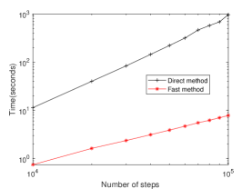
(a) Computational time

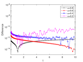
(b) Difference

Figure 1: (a): The computational time of the fast method and direct method; (b): The difference between the numerical solutions of the fast method and direct method; Example 4.1, $Q=256$, $M=10000$, $r=2$, $p=1$.

Table 2: The average error for Example 4.1 when $p=2$.

$\alpha$	$N$	$r=2$		$r=2.2$		$r=2.5$		$r=\frac{6-\alpha}{1+\alpha}$		$r=5$
		Error	Rate	Error	Rate	Error	Rate	Error	Rate	Error	Rate
	32	6.98e-04	-	4.11e-04	-	2.01e-04	-	2.75e-05	-	2.81e-05	-
	64	2.86e-04	1.29	1.53e-04	1.42	6.45e-05	1.64	3.98e-06	2.79	4.06e-06	2.79
0.2	128	1.15e-04	1.31	5.61e-05	1.45	2.03e-05	1.67	5.54e-07	2.84	5.63e-07	2.85
	256	4.62e-05	1.32	2.03e-05	1.47	6.32e-06	1.69	7.54e-08	2.88	7.65e-08	2.88
	512	1.83e-05	1.34	7.29e-06	1.48	1.94e-06	1.70	1.01e-08	2.90	1.02e-08	2.90
	32	2.33e-04	-	1.16e-04	-	4.31e-05	-	5.81e-06	-	6.13e-06	-
	64	7.37e-05	1.66	3.19e-05	1.86	9.61e-06	2.17	8.62e-07	2.75	1.05e-06	2.54
0.5	128	2.23e-05	1.72	8.39e-06	1.93	2.03e-06	2.24	1.21e-07	2.83	1.66e-07	2.66
	256	6.55e-06	1.77	2.13e-06	1.98	4.12e-07	2.30	1.65e-08	2.88	2.43e-08	2.77
	512	1.87e-06	1.81	5.27e-07	2.02	8.16e-08	2.34	2.19e-09	2.91	3.38e-09	2.85
	32	4.04e-05	-	1.72e-05	-	4.86e-06	-	1.76e-06	-	6.77e-06	-
	64	1.11e-05	1.87	4.09e-06	2.08	9.25e-07	2.39	2.39e-07	2.88	9.03e-07	2.91
0.8	128	2.91e-06	1.93	9.28e-07	2.14	1.69e-07	2.46	3.15e-08	2.92	1.17e-07	2.95
	256	7.47e-07	1.96	2.06e-07	2.17	3.01e-08	2.48	4.11e-09	2.94	1.50e-08	2.97
	512	1.89e-07	1.98	4.53e-08	2.19	5.34e-09	2.50	5.33e-10	2.95	1.89e-09	2.98

Table 3: The average error in time for Example 4.2 when $p=1$ and $h=1/256$.

$\alpha$	$N$	$r=1$		$r=1.2$		$r=1.6$		$r=\frac{4-\alpha}{1+\alpha}$		$r=3.5$
		Error	Rate	Error	Rate	Error	Rate	Error	Rate	Error	Rate
	32	1.94e-01	-	1.32e-01	-	6.14e-02	-	6.79e-03	-	6.12e-03	-
	64	1.14e-01	0.77	7.00e-02	0.92	2.65e-02	1.21	1.54e-03	2.14	1.39e-03	2.13
0.2	128	6.68e-02	0.77	3.71e-02	0.92	1.15e-02	1.21	3.56e-04	2.11	3.29e-04	2.08
	256	3.93e-02	0.76	1.97e-02	0.91	4.97e-03	1.21	8.37e-05	2.09	7.98e-05	2.05
	512	2.32e-02	0.76	1.05e-02	0.91	2.16e-03	1.21	2.00e-05	2.06	1.96e-05	2.02
	32	4.69e-02	-	2.46e-02	-	6.83e-03	-	1.78e-03	-	2.20e-03	-
	64	2.12e-02	1.15	9.47e-03	1.38	1.90e-03	1.85	4.40e-04	2.02	5.66e-04	1.96
0.5	128	9.50e-03	1.16	3.57e-03	1.41	5.06e-04	1.91	1.08e-04	2.02	1.44e-04	1.98
	256	4.20e-03	1.18	1.30e-03	1.45	1.30e-04	1.96	2.69e-05	2.01	3.62e-05	1.99
	512	1.82e-03	1.21	4.61e-04	1.50	3.25e-05	2.00	6.68e-06	2.01	9.09e-06	1.99
	32	1.17e-02	-	4.74e-03	-	1.22e-03	-	1.15e-03	-	3.16e-03	-
	64	3.76e-03	1.64	1.15e-03	2.04	2.60e-04	2.23	2.81e-04	2.03	8.44e-04	1.90
0.8	128	1.12e-03	1.74	2.53e-04	2.19	6.23e-05	2.06	7.09e-05	1.99	2.19e-04	1.95
	256	3.16e-04	1.83	5.15e-05	2.30	1.57e-05	1.99	1.79e-05	1.99	5.59e-05	1.97
	512	8.51e-05	1.89	1.04e-05	2.31	3.97e-06	1.98	4.51e-06	1.99	1.42e-05	1.98

Example 4.2.

Consider the following initial-boundary value problem

(69) $$\left\{\begin{aligned} &{}_{0}^{C}D_{t}^{\alpha}u(x,t)=\Delta u(x,t)+f(x,t),\quad(x,t)\in\Omega\times(0,T],T>0,\\ &u(x,0)=\sin(x),\quad x\in\bar{\Omega},\\ &u(x,t)=0,\quad(x,t)\in\partial\Omega\times[0,T],\end{aligned}\right.$$

where $\Omega=(0,1)$ and $0<\alpha<1$. The exact solution to (4.2) is $u=(1+t^{\alpha}+t^{2\alpha})\sin(2\pi x)$ when

$$f(t)=(4\pi^{2}+\Gamma(\alpha+1)+(4\pi^{2}+\Gamma(2\alpha+1)/\Gamma(\alpha+1))t^{\alpha}+4\pi^{2}t^{2\alpha})\sin(2\pi x).$$

Table 4: The average error in space for Example 4.2 when $p=1$ and $N=20000$.

$\alpha$	$h$	$r=1$		$r=1.2$		$r=1.6$		$r=\frac{4-\alpha}{1+\alpha}$		$r=3.5$
		Error	Rate	Error	Rate	Error	Rate	Error	Rate	Error	Rate
	1/4	4.04e-01	-	4.04e-01	-	4.04e-01	-	4.04e-01	-	4.04e-01	-
	1/8	1.24e-01	1.70	1.24e-01	1.70	1.24e-01	1.70	1.24e-01	1.70	1.24e-01	1.70
0.2	1/16	3.26e-02	1.93	3.26e-02	1.93	3.26e-02	1.93	3.26e-02	1.93	3.26e-02	1.93
	1/32	8.35e-03	1.97	8.24e-03	1.98	8.23e-03	1.98	8.23e-03	1.98	8.23e-03	1.98
	1/64	2.48e-03	1.75	2.09e-03	1.98	2.06e-03	2.00	2.06e-03	2.00	2.06e-03	2.00
	1/4	3.41e-01	-	3.41e-01	-	3.41e-01	-	3.41e-01	-	3.41e-01	-
	1/8	1.05e-01	1.71	1.05e-01	1.71	1.05e-01	1.71	1.05e-01	1.71	1.05e-01	1.71
0.5	1/16	2.73e-02	1.93	2.73e-02	1.93	2.73e-02	1.93	2.73e-02	1.93	2.73e-02	1.93
	1/32	6.91e-03	1.98	6.91e-03	1.98	6.91e-03	1.98	6.91e-03	1.98	6.91e-03	1.98
	1/64	1.73e-03	2.00	1.73e-03	2.00	1.73e-03	2.00	1.73e-03	2.00	1.73e-03	2.00
	1/4	2.87e-01	-	2.87e-01	-	2.87e-01	-	2.87e-01	-	2.87e-01	-
	1/8	8.69e-02	1.72	8.69e-02	1.72	8.69e-02	1.72	8.69e-02	1.72	8.69e-02	1.72
0.8	1/16	2.27e-02	1.94	2.27e-02	1.94	2.27e-02	1.94	2.27e-02	1.94	2.27e-02	1.94
	1/32	5.72e-03	1.99	5.72e-03	1.99	5.72e-03	1.99	5.72e-03	1.99	5.72e-03	1.99
	1/64	1.43e-03	2.00	1.43e-03	2.00	1.43e-03	2.00	1.43e-03	2.00	1.43e-03	2.00

Considering $T=4$, we employ linear DG and linear FEM in the computation. Table 3 gives the average errors and convergence rates in time of Example 4.2 when $\alpha=0.2,0.5$ and $0.8$, respectively, for various choices of $N$ and $r$. The optimal rates of order $O(N^{-2})$ is observed when $r\geq\frac{2p+2-\alpha}{1+2\sigma-\alpha}$. The errors and convergence rates in space are displayed in Table 4, which second-order accuracy is observed. The numerical results are consistent with Theorem 2.2.

5 Conclusion

This work develops a high-order fast time-stepping DG FEM for the subdiffusion equation. We prove the optimal error estimate of the time-stepping DG method, which displays that the error in the $L^{2}((0,T),L^{2}(\Omega))$-norm is $O(N^{-p-1}+h^{m+1}+\varepsilon N^{r\alpha})$. Our result improves the error bound in [24]. Numerical examples are given to demonstrate the theoretical analysis.

Appendix A Proof of Lemma 2.3

For any function $v\in C([0,T])$, the piecewise Lagrange interpolant $\Pi^{p}v$ is defined by

$$\Pi^{p}v(t_{n,j})=v(t_{n,j}),\quad t_{n,j}\in[t_{n-1},t_{n}],\quad 0\leq j\leq p,\quad 1\leq n\leq N,$$

where $\Pi^{p}v(t)|_{t\in[t_{n-1},t_{n}]}$ is the polynomial with degree $p$, $t_{n,j}=t_{n-1}+j\tau_{n}/p,0\leq j\leq p$, $p\geq 1$. Denote the interpolation error as $\eta_{v}=v-\Pi^{p}v$.

Denote the right-hand-side RL integral operator ${}_{t}\partial_{b}^{-\alpha}$ as

$${}_{t}\partial_{b}^{-\alpha}v(t)=\int_{t}^{b}\frac{(s-t)^{\alpha-1}}{\Gamma(\alpha)}v(s)\textrm{d}s,\quad\alpha\geq 0.$$

Then, ${}_{t}\partial_{b}^{\alpha}$ denotes the right-hand-side RL derivative operator of order $\alpha$ in the sense of the principal value [27].

Let $J_{n}=(0,t_{n})$. Let $J_{L}^{\alpha}(J_{n})$ and $J_{R}^{\alpha}(J_{n})$ be the left and right factional derivative spaces, respectively. Define the semi-norms $|\cdot|_{J_{L}^{\alpha}(J_{n})}$ and $|\cdot|_{J_{R}^{\alpha}(J_{n})}$, respectively, by

$$|v|_{J_{L}^{\alpha}(J_{n})}=\left(\int_{0}^{t_{n}}|\partial_{t}^{\alpha}v(t)|^{2}\textrm{d}t\right)^{1/2}\quad\text{and}\quad|v|_{J_{R}^{\alpha}(J_{n})}=\left(\int_{0}^{t_{n}}|{}_{t}\partial_{t_{n}}^{\alpha}v(t)|^{2}\textrm{d}t\right)^{1/2}.$$

The norms $\|\cdot\|_{J_{L}^{\alpha}(J_{n})}$ and $\|\cdot\|_{J_{R}^{\alpha}(J_{n})}$ are, respectively, defined by

$$\|v\|_{J_{L}^{\alpha}(J_{n})}=\left(|v|_{J_{L}^{\alpha}(J_{n})}^{2}+\|v\|^{2}_{L^{2}(J_{n})}\right)^{1/2}\text{ and }\|v\|_{J_{R}^{\alpha}(J_{n})}=\left(|v|_{J_{R}^{\alpha}(J_{n})}^{2}+\|v\|^{2}_{L^{2}(J_{n})}\right)^{1/2},$$

where $\|v\|^{2}_{L^{2}(J_{n})}=\int_{0}^{t_{n}}|v(t)|^{2}\textrm{d}t=|v|_{J_{L}^{0}(J_{n})}.$ Readers can refer to [26] for details.

Lemma A.1.

Let $\alpha_{1}+\alpha_{2}=\alpha<1$, $\alpha_{1},\alpha_{2}\geq 0$, $w\in J_{L}^{\alpha}(J_{n})$, $v\in J_{R}^{\alpha_{2}}(J_{n})$. Then

$$\int_{0}^{t_{n}}v(t)\partial_{t}^{\alpha}w(t)\textrm{d}t=\int_{0}^{t_{n}}\partial_{t}^{\alpha_{1}}w(t){}_{t}\partial_{t_{n}}^{\alpha_{2}}v(t)\textrm{d}t.$$

Proof.

The proof is similar to that of [26, Lemma 3.1.4], the details are omitted. The proof is complete. ∎

Lemma A.2.

Let $v\in J_{L}^{\alpha}(J_{n}),0<\alpha<1/2$. Then

$$|v|_{J_{L}^{\alpha}(J_{n})}^{2}\lesssim\Big{|}\int_{0}^{t_{n}}\partial_{t}^{\alpha}v(t){}_{t}\partial_{t_{n}}^{\alpha}v(t)\textrm{d}t\Big{|}\lesssim|v|_{J_{R}^{\alpha}(J_{n})}^{2}\lesssim|v|_{J_{L}^{\alpha}(J_{n})}^{2}.$$

Proof.

Following the proofs of Theorems 3.1.3, 3.1.5, and 3.1.13 in [26] yields the desired result. The proof is complete. ∎

Lemma A.3.

Let $v\in J_{R}^{\gamma}(J_{n})\cap C(\bar{J}_{n})$. Then

$$\|\Pi^{p}v-v\|_{J_{R}^{\beta}(J_{n})}\lesssim N^{\beta-\gamma}\|v\|_{J_{R}^{\gamma}(J_{n})},\quad 0\leq\beta\leq\gamma\leq 2.$$

Proof.

The above error bound follows from $\|\Pi^{p}v-v\|_{J_{R}^{\beta}(J_{n})}\lesssim\|\Pi^{p}v-v\|_{H^{\beta}(J_{n})}\lesssim N^{\beta-\gamma}\|v\|_{H^{\gamma}(J_{n})}\lesssim N^{\beta-\gamma}\|v\|_{J_{R}^{\gamma}(J_{n})}$, see [26, Theorem 3.1.13] and [26, Theorem 3.3.2] (or [5, Eq. (4.2.21)]). The proof is complete. ∎

Lemma A.4.

Let $v\in C([0,T])$ and satisfy

(70) $$|v(t)-v(0)|\lesssim t^{\sigma},\quad|v^{(\ell)}(t)|\lesssim 1+t^{\sigma-\ell},\quad t>0,0<\sigma<1,0\leq\ell\leq p+1.$$

Then

(71) $$|\eta_{v}(t)|\lesssim t_{n}^{\sigma-p-1}(t-t_{n})^{p+1}, \quad t\in[t_{n},t_{n+1}],n\geq 1,$$

$$|\eta^{\prime}_{v}(t)|\lesssim t_{n}^{\sigma-p-1}(t-t_{n})^{p}, \quad t\in[t_{n},t_{n+1}],n\geq 1$$

$$|\eta^{\prime}_{v}(t)|\lesssim t_{1}^{\sigma-1}+t^{\sigma-1}, \quad t\in[0,t_{1}].$$

Proof.

For each $n\geq 1$, let $T_{p}^{n}v(t)=\sum_{k=0}^{p}\frac{v^{(k)}(t_{n})}{k!}(t-t_{n})^{k}$ be the Taylor polynomial of order $p$ of $v(t)$, satisfying

(72) $$v(t)-T_{p}^{n}v(t)=\int_{t_{n}}^{t}\frac{v^{(p+1)}(s)}{p!}(t-s)^{p}\textrm{d}s.$$

By $|\Pi^{p}(T_{p}^{n}v-v)|\lesssim|T_{p}^{n}v-v|$, the inverse inequality $|(\Pi^{p}(T_{p}^{n}v-v))^{\prime}|\lesssim\tau_{n+1}^{-1}|T_{p}^{n}v-v|$ (see [5, Eq. (4.5.4)])) for $t\in[t_{n},t_{n+1}]$, and the following relation

(73) $$\eta_{v}(t)=v(t)-\Pi^{p}v(t)=(v(t)-T_{p}^{n}v(t))+\Pi^{p}(T_{p}^{n}v(t)-v(t)),$$

we have

(74) $$|\eta_{v}(t)|\lesssim |v(t)-T_{p}^{n}v(t)|,$$

$$|(\eta_{v}(t))^{\prime}|\lesssim |(v(t)-T_{p}^{n}v(t))^{\prime}|+\tau_{n+1}^{-1}|(T_{p}^{n}v(t)-v(t))|.$$

For $t\in[t_{n},t_{n+1}]$, $n\geq 1$, by (74), (72), and (70), we obtain

(75) $$|\eta_{v}(t)|\lesssim \int_{t_{n}}^{t}|v^{(p+1)}(s)|(t-s)^{p}\textrm{d}s\lesssim t_{n}^{\sigma-p-1}(t-t_{n})^{p+1},$$

$$|\eta^{\prime}_{v}(t)|\lesssim \int_{t_{n}}^{t}|v^{(p+1)}(s)|(t-s)^{p-1}\textrm{d}s\lesssim t_{n}^{\sigma-p-1}(t-t_{n})^{p}.$$

For $t\in[0,t_{1}]$, by $\eta_{v}=v-\Pi^{1}v+\Pi^{1}v-\Pi^{p}v$, the inverse inequality $|(\Pi^{1}v-\Pi^{p}v)^{\prime}|\lesssim\tau_{1}^{-1}|\Pi^{1}v-\Pi^{p}v|$, $(\Pi^{1}v)^{\prime}=(v(t_{1})-v(0))/\tau_{1}$, we derive

(76) $$|\eta^{\prime}_{v}|= |(v-\Pi^{1}v)^{\prime}+(\Pi^{1}v-\Pi^{p}v)^{\prime}|\lesssim|(v-\Pi^{1}v)^{\prime}|+\tau_{1}^{-1}|\Pi^{1}v-\Pi^{p}v|$$

$$\lesssim \tau_{1}^{-1}|v(t_{1})-v(0)|+|v^{\prime}(t)|+\tau_{1}^{-1}|v(t)-v(0)|$$

$$\lesssim t_{1}^{\sigma-1}+t^{\sigma-1}+t_{1}^{-1}t^{\sigma}\lesssim t_{1}^{\sigma-1}+t^{\sigma-1}.$$

The proof is complete. ∎

Lemma A.5.

Let $v$ satisfy (70). Then

(77) $$\int_{0}^{t_{k-2}}{(t_{k-1}-s)^{-\alpha-1}}|\eta_{v}(s)|\textrm{d}s\lesssim\Phi(k,N,r,\alpha,\sigma,p),\quad k\geq 2,$$

where

(78) $$\Phi(k,N,r,\alpha,\sigma,p)=t_{k}^{\sigma-\alpha}\left\{\begin{aligned} &k^{-(p+1-\alpha)},&&r(1+\sigma)\geq p+1,\\ &k^{-r(1+\sigma)},&&r(1+\sigma)<p+1.\end{aligned}\right.$$

Proof.

With (71), the error bound (77) can be similarly proved as that of the case $p=1$, the details are omitted, see [28, Lemma 2.1]. The proof is complete. ∎

Lemma A.6.

Let $v$ satisfy (70). For $t\in[t_{k-1},t_{k}],k\geq 1$, we have

(79) $$\int_{t_{k-1}}^{t_{k}}|\partial_{t}^{\alpha}\eta_{v}(t)|^{2}\textrm{d}t\lesssim\tau_{k}(\Phi(k,N,r,\alpha,\sigma,p))^{2}.$$

Proof.

By $\eta_{v}(0)=0$ and (9), $\partial_{t}^{\alpha}\eta_{v}(t)=\partial_{t}^{\alpha-1}(\eta_{v})^{\prime}(t)$. For $t\in[t_{0},t_{1}]$, by (76),

(80) $$|\partial_{t}^{\alpha}\eta_{v}(t)|= \bigg{|}\int_{0}^{t}\frac{(t-s)^{-\alpha}}{\Gamma(1-\alpha)}(\eta_{v})^{\prime}(s)\textrm{d}s\bigg{|}\leq\int_{0}^{t}\frac{(t-s)^{-\alpha}}{\Gamma(1-\alpha)}|(\eta_{v})^{\prime}(s)|\textrm{d}s$$

$$\lesssim \int_{0}^{t}\frac{(t-s)^{-\alpha}}{\Gamma(1-\alpha)}(t_{1}^{\sigma-1}+s^{\sigma-1})\textrm{d}s\lesssim t_{1}^{\sigma-1}t^{1-\alpha}+t^{\sigma-\alpha}.$$

Hence, $\int_{0}^{t_{1}}|\partial_{t}^{\alpha}\eta_{v}(t)|^{2}\textrm{d}t\lesssim t_{1}^{2\sigma-2\alpha+1}\lesssim\tau_{1}(\Phi(1,N,r,\alpha,\sigma,p))^{2}.$

By the similar reasoning, (80) holds for $t\in[t_{1},t_{2}]$, which leads to $\int_{0}^{t_{2}}|\partial_{t}^{\alpha}\eta_{v}(t)|^{2}\textrm{d}t\lesssim t_{2}^{2\sigma-2\alpha+1}\lesssim\tau_{2}(\Phi(2,N,r,\alpha,\sigma,p))^{2}.$

For $t\in[t_{k-1},t_{k}],k\geq 3$, using (9) with $\eta_{v}(t_{k-2})=0$, we have

(81) $$\partial_{t}^{\alpha}\eta_{v}(t)= \underbrace{\int_{0}^{t_{k-2}}\frac{(t-s)^{-\alpha-1}}{\Gamma(-\alpha)}\eta_{v}(s)\textrm{d}s}_{J_{1}}+\underbrace{\int_{t_{k-2}}^{t}\frac{(t-s)^{-\alpha}}{\Gamma(1-\alpha)}(\eta_{v}(s))^{\prime}\textrm{d}s}_{J_{2}}.$$

By $(t-s)^{-\alpha-1}\leq(t_{k-1}-s)^{-\alpha-1}$ for $(t,s)\in[t_{k-1},t_{k}]\times[0,t_{k-2}]$ and Lemma A.5, we have

(82) $$|J_{1}|\leq \int_{0}^{t_{k-2}}\frac{(t_{k-1}-s)^{-\alpha-1}}{|\Gamma(-\alpha)|}|\eta_{v}(s)|\textrm{d}s\lesssim\Phi(k,N,r,\alpha,\sigma,p).$$

By Lemma A.4, we can easily derive

(83) $$|J_{2}|\leq \int_{t_{k-2}}^{t}\frac{(t-s)^{-\alpha}}{\Gamma(1-\alpha)}|\eta^{\prime}_{v}(s)|\textrm{d}s\lesssim(t-t_{k-2})^{1-\alpha}\tau_{k}^{p}t_{k-2}^{\sigma-p-1}$$

$$\lesssim \tau_{k}^{p+1-\alpha}t_{k}^{\sigma-p-1}\lesssim\Phi(k,N,r,\alpha,\sigma,p).$$

Combining (81)–(83) yields $|\partial_{t}^{\alpha}\eta_{v}(t)|\leq|J_{1}|+|J_{2}|\lesssim\Phi(k,N,r,\alpha,\sigma,p)$, which leads to (79) for $k\geq 3$. The proof is complete. ∎

Lemma A.7.

Let $t\in[t_{n-1},t_{n}]$ and $1\leq n\leq N$. If $v$ satisfies (70) and $\sigma\leq p+(p+1)/\alpha$, then

(84) $$\int_{0}^{t_{n}}|\partial_{t}^{\alpha/2}\eta_{v}(t)|^{2}\textrm{d}t\lesssim\left\{\begin{aligned} &N^{-r(1+2\sigma-\alpha)},&&1\leq r<\frac{2p+2-\alpha}{1+2\sigma-\alpha},\\ &N^{-2p-2+\alpha}(1+\ln(n)),&&r=\frac{2p+2-\alpha}{1+2\sigma-\alpha},\\ &N^{-2p-2+\alpha}t_{n}^{1+2\sigma-\alpha-\frac{2p+2-\alpha}{r}},&&r>\frac{2p+2-\alpha}{1+2\sigma-\alpha}.\end{aligned}\right.$$

Proof.

Using Lemma A.6 yields

$$\int_{0}^{t_{n}}|\partial_{t}^{\alpha/2}\eta_{v}(t)|^{2}\textrm{d}t= \sum_{k=1}^{n}\int_{t_{k-1}}^{t_{k}}|\partial_{t}^{\alpha/2}\eta_{v}(t)|^{2}\textrm{d}t\lesssim\sum_{k=1}^{n}\tau_{k}(\Phi(k,N,r,\alpha/2,\sigma,p))^{2}.$$

Case $r(1+\sigma)\geq p+1$. By $\tau_{k}\lesssim k^{r-1}N^{-r}$ and $t_{k}\lesssim k^{r}N^{-r}$, we have

(85) $$\sum_{k=1}^{n}\tau_{k}\left(\Phi(k,N,r,\alpha/2,\sigma,p)\right)^{2}= \sum_{k=1}^{n}k^{-(2p+2-\alpha)}\tau_{k}t_{k}^{2\sigma-\alpha}$$

$$\lesssim \sum_{k=1}^{n}k^{-(2p+2-\alpha)}k^{r-1}N^{-r}(k^{r}N^{-r})^{2\sigma-\alpha}$$

$$= N^{-r(1+2\sigma-\alpha)}\sum_{k=1}^{n}k^{r(1+2\sigma-\alpha)-(2p+3-\alpha)}.$$

Direct calculations show that

(86) $$\sum_{k=1}^{n}k^{r(1+2\sigma-\alpha)-(2p+3-\alpha)}\lesssim\left\{\begin{aligned} &n^{r(1+2\sigma-\alpha)-(2p+2-\alpha)}&&\mathrm{if}\ \ r(1+2\sigma-\alpha)>2p+2-\alpha,\\ &\ln(n+1)&&\mathrm{if}\ \ r(1+2\sigma-\alpha)=2p+2-\alpha,\\ &1&&\mathrm{if}\ \ r(1+2\sigma-\alpha)<2p+2-\alpha.\end{aligned}\right.$$

Combining (85) and (86) yields (84).

Case $r(1+\sigma)<p+1$. We have

$$\sum_{k=1}^{n}\tau_{k}\left(\Phi(k,N,r,\alpha/2,\sigma,p)\right)^{2}= \sum_{k=1}^{n}\tau_{k}k^{-2r(1+\sigma)}t_{k}^{2\sigma-\alpha}$$

$$\lesssim N^{-r(2\sigma-\alpha)}\sum_{k=1}^{n}k^{r-1}N^{-r}k^{-2r(1+\sigma)}k^{r(2\sigma-\alpha)}$$

$$= N^{-r(1+2\sigma-\alpha)}\sum_{k=1}^{n}k^{-1-r(\alpha+1)}\lesssim N^{-r(1+2\sigma-\alpha)}.$$

The proof is complete. ∎

Now, we are in a position to prove Lemma 2.3.

Proof.

Denote $P_{m}(I_{k})$ be the polynomial space of degree $m$ on $I_{k}$ and $\mathcal{P}_{m}(J_{n})=\{v\in L^{2}(J_{n}):v|_{I_{k}}\in P_{m}(I_{k}),\ 1\leq k\leq n\}$. Let $e(t)=R_{t}^{\alpha}v(t)-v(t)$, $\theta(t)=R_{t}^{\alpha}v(t)-\Pi^{p}v(t)$, and $\eta_{v}(t)=\Pi^{p}v(t)-v(t)$. Then, $e(t)=\theta(t)+\eta_{v}(t)$ and

$$\int_{0}^{t_{n}}X(t)\partial_{t}^{\alpha}\theta(t)\textrm{d}t=-\int_{0}^{t_{n}}X(t)\partial_{t}^{\alpha}\eta_{v}(t)\textrm{d}t,\qquad X\in\mathcal{P}_{m}(J_{n}).$$

Letting $X(t)=\theta(t)$ in the above equation, and using Lemmas A.1 and A.2, we obtain

(87) $$\int_{0}^{t_{n}}|\partial_{t}^{\alpha/2}\theta(t)|^{2}\textrm{d}t\lesssim \int_{0}^{t_{n}}\theta(t)\partial_{t}^{\alpha}\theta(t)\textrm{d}t=-\int_{0}^{t_{n}}{}_{t}\partial_{t_{n}}^{\alpha/2}\theta(t)\partial_{t}^{\alpha/2}\eta_{v}(t)\textrm{d}t$$

$$\lesssim \left(\int_{0}^{t_{n}}|{}_{t}\partial_{t_{n}}^{\alpha/2}\theta(t)|^{2}\textrm{d}t\right)^{1/2}\left(\int_{0}^{t_{n}}|\partial_{t}^{\alpha/2}\eta_{v}(t)|^{2}\textrm{d}t\right)^{1/2}$$

$$\lesssim |\theta|_{J_{L}^{\alpha/2}(J_{n})}|\eta_{v}|_{J_{L}^{\alpha/2}(J_{n})}.$$

The above inequality yields $|\theta|_{J_{L}^{\alpha/2}(J_{n})}\lesssim|\eta_{v}|_{J_{L}^{\alpha/2}(J_{n})}$. Using the triangular inequality $|e|_{J_{L}^{\alpha/2}(J_{n})}\leq|\theta|_{J_{L}^{\alpha/2}(J_{n})}+|\eta_{v}|_{J_{L}^{\alpha/2}(J_{n})}$ and Lemma A.7, we obtain

(88) $$|e|_{J_{L}^{\alpha/2}(J_{n})}^{2}\lesssim N^{\alpha}\mathcal{E}(n,N,\sigma,\alpha,r,p).$$

Introduce $w$ as the solution to the adjoint problem

(89) $${}_{t}\partial_{t_{n}}^{\alpha}w(t)=e(t),\qquad w(t_{n})=0.$$

By Lemma A.2 and the above equation, $w$ satisfies

(90) $$\|w\|_{J_{L}^{\alpha}(J_{n})}\lesssim\|w\|_{J_{R}^{\alpha}(J_{n})}\lesssim\|e\|_{L^{2}(J_{n})}.$$

Multiplying $e(t)$ on both sides of (89) and integrating over $J_{n}$, we obtain

(91) $$\|e\|^{2}_{L^{2}(J_{n})}= \int_{0}^{t_{n}}e(t){}_{t}\partial_{t_{n}}^{\alpha}w(t)\textrm{d}t=\int_{0}^{t_{n}}w(t)\partial_{t}^{\alpha}e(t)\textrm{d}t\qquad\text{(By Lemma \ref{lemA2})}$$

$$= \int_{0}^{t_{n}}(w(t)-\Pi^{p}w(t))\,\partial_{t}^{\alpha}e(t)\textrm{d}t\qquad(\text{By \eqref{Rtalf}})$$

$$= -\int_{0}^{t_{n}}{}_{t}\partial_{t_{n}}^{\alpha/2}\eta_{w}(t)\,\partial_{t}^{\alpha/2}e(t)\textrm{d}t\qquad\text{(By Lemma \ref{lemA2})}$$

$$\leq |e|_{J_{L}^{\alpha/2}(J_{n})}|\eta_{w}|_{J_{R}^{\alpha/2}(J_{n})}$$

$$\lesssim N^{-\alpha/2}|e|_{J_{L}^{\alpha/2}(J_{n})}\|w\|_{J_{R}^{\alpha}(J_{n})}\qquad\text{(By Lemma \ref{lemA3})}$$

$$\lesssim N^{-\alpha/2}|e|_{J_{L}^{\alpha/2}(J_{n})}\|e\|_{L^{2}(J_{n})}.\qquad\text{(By \eqref{eq:A17})}$$

The above inequality and (88) yield (18). The proof is complete. ∎