Maximal Cliques in Scale-Free Random Graphs

Abstract

We investigate the number of maximal cliques, i.e., cliques that are not contained in any larger clique, in three network models: Erdős–Rényi random graphs, inhomogeneous random graphs (also called Chung–Lu graphs), and geometric inhomogeneous random graphs. For sparse and not-too-dense Erdős–Rényi graphs, we give linear and polynomial upper bounds on the number of maximal cliques. For the dense regime, we give super-polynomial and even exponential lower bounds. Although (geometric) inhomogeneous random graphs are sparse, we give super-polynomial lower bounds for these models. This comes form the fact that these graphs have a power-law degree distribution, which leads to a dense subgraph in which we find many maximal cliques. These lower bounds seem to contradict previous empirical evidence that (geometric) inhomogeneous random graphs have only few maximal cliques. We resolve this contradiction by providing experiments indicating that, even for large networks, the linear lower-order terms dominate, before the super-polynomial asymptotic behavior kicks in only for networks of extreme size.

1 Introduction

While networks appear in many different applications, many real-world networks were found to share some important characteristics. First of all, often their degree distribution is heavy-tailed, which is sometimes denoted as the network being scale-free. Secondly, they often have a high clustering coefficient, implying that it is likely that two neighbors of a vertex are connected themselves as well. For this reason, random graph models that can achieve both scale-freeness and a high clustering coefficient have been at the center of attention over the last years.

One example of such a model is the popular hyperbolic random graph (HRG) [16], which has for example been used to model the network of world wide trade [11] or the Internet on the Autonomous Systems level [6, 15]. This random graph model embeds the vertices in an underlying hyperbolic space and connects them with probabilities depending on their distances, where nearby vertices are more likely to connect. The triangle inequality then ensures the presence of many triangles, while the hyperbolic space ensures the presence of a scale-free degree distribution. Recently, the geometric inhomogeneous random graph (GIRG) was proposed as a generalization of HRG. It combines power-law distributed weights with Euclidean space, making the model simpler to analyze [7].

While the hyperbolic random graph and the GIRG have been designed to exhibit high clustering and a scale-free degree distribution, the question remains whether other properties of this model match real-world data. For this reason, many properties of the GIRG or hyperbolic random graph have been analyzed mathematically, such as the maximum clique size [2], number of $k$-cliques [18], spectral gap [14] and separator size [5, 17].

In this paper, we focus on another network property: the number of maximal cliques, i.e., cliques that are not part of any larger clique. Cliques in general are an important indicator for structural properties of a network. Indeed, the number of large cliques is a measure of the tendency of a network to cluster into groups. Small cliques of size 3 (triangles) on the other hand, can form an indication of the transitivity of a network or its clustering coefficient.

To study these structural clique-based properties, however, all cliques of a given size need to be listed, which can be a computationally expensive process. To list all network cliques, it suffices to list only all maximal cliques, as all smaller cliques can be generated from at least one maximal clique. For this reason, enumerating all maximal cliques of a graph is at the heart of our understanding of cliques in general.

For enumerating all maximal cliques, an output-polynomial algorithm [19] exists, which can enumerate all maximal cliques efficiently if the graph contains only few of them. There also exist highly efficient implementations to enumerate all maximal cliques [8, 9, 10]. However, for a given graph, it is usually not known a priori how many maximal cliques it has. If this number is large, enumerating all maximal cliques can still take exponential time. However, in practice, enumerating the number of maximal cliques often takes a short amount of time for many real-world instances as well as in realistic network models [3]. In this paper, we therefore focus on the number of maximal cliques in the GIRG random graph. As the GIRG possesses the two main characteristics that are essential to many real-world networks, scale-freeness and an underlying geometry, we believe that investigating the number of maximal cliques in the GIRG can provide insights into in why enumerating the number of maximal cliques can often be done efficiently for many real-world networks.

To investigate the influence of the different properties of scale-freeness and clustering, we investigate the number of maximal cliques in three steps. First, we investigate a model without heavy-tailed degrees and with a small clustering coefficient, the Erdős–Rényi model $G(n,p)$; see Section 2. We then investigate the GIRG model (Section 3), which has both clustering and scale-free degrees. Finally, in Section 4, we investigate the Inhomogeneous Random Graph (IRG), a model that is scale-free but has a small clustering coefficient. We complement our theoretical bounds with experiments in Section 5. Our main findings can be summarized as follows; also see Table 1 for an overview of our results.

• There is a strong dependence on the density of the network. For the Erdős–Rényi model ($G(n,p)$) we obtain a linear upper bound for sparse graphs ($O(n)$ edges) and a polynomial upper bound for non-dense graphs ($O(n^{2-\varepsilon})$ edges for any $\varepsilon>0$). For dense graphs on the other hand ($\Omega(n^{2})$ edges), we obtain a super-polynomial lower bound. If the density is high enough, our lower bound is even exponential.

• This insight carries over to the IRG and GIRG models. Though they are overall sparse, they contain sufficiently large dense subgraphs that allow us to obtain super-polynomial lower bounds.

• In the IRG model with power-law exponent $\tau\in(2,3)$ the small maximal cliques localize: asymptotically maximal cliques of constant size $k>2$ are formed by $k-2$ hubs of high degree proportional to $n^{1/(\tau-1)}$ and two vertices of lower degree proportional to $n^{(\tau-2)/(\tau-1)}$.

• We complement our theoretical lower bounds with experiments showing that the super-polynomial growth becomes only relevant for very large networks.

Discussion and Related Work.

Although cliques themselves have been studied extensively in the literature, there is, to the best of our knowledge, only little previous work on the number of maximal cliques in network models. In fact, the only theoretical analysis we are aware of is the recent preprint by Yamaji [20], giving bounds for hyperbolic random graphs (HRG) and random geometric graph (RGG), which are also shown in Table 1. Interestingly, this includes the upper bound of $\exp(O(n^{\frac{3-\tau}{6}+\varepsilon}))$ for the HRG model. In contrast to that, we give the asymptotically larger lower bound $\exp(\Omega(n^{\frac{3-\tau}{4}-\varepsilon}))$ for the corresponding GIRG variant. Thus, there is an asymptotic difference between the HRG and the GIRG model.

This is surprising as the GIRG model is typically perceived as a generalization of the HRG model. More precisely, there is a mapping between the two models such that for every HRG with average degree $d_{\mathrm{HRG}}$ there exist GIRGs with average degree $d_{\mathrm{GIRG}}$ and $D_{\mathrm{GIRG}}$ with $d_{\mathrm{GIRG}}\leq d_{\mathrm{HRG}}\leq D_{\mathrm{GIRG}}$ that are sub- and supergraphs of the HRG, respectively. Moreover, $d_{\mathrm{GIRG}}$ and $D_{\mathrm{GIRG}}$ are only a constant factor apart and experiments indicate that $d_{\mathrm{HRG}}=d_{\mathrm{GIRG}}\cdot(1+o(1))$, i.e., every HRG has a corresponding GIRG that is missing only a sublinear number of edges [4]. In the case of maximal cliques, however, this minor difference between the models leads to an asymptotic difference.

Besides this theoretical analysis, it has been observed empirically that the number of maximal cliques in most real-world networks as well as in the GIRG and the IRG model is smaller than the number of edges of the graph [3]. This indicates linear scaling in the graph size with low constant factors and small lower-order terms, which seems to be a stark contradiction to the super-polynomial lower bounds we prove here. We resolve this contradiction with our experiments in Section 5, where we observe that the graph size has to be quite large before the asymptotic behavior kicks in, i.e., we observe the super-polynomial scaling as predicted by our theorems but on such a low level that it is overshadowed by the linear lower-order terms.

Model		Maximal cliques	Reference
$G(n,p)$	$p=1-\Theta(\frac{1}{n})$	$2^{\Omega(n)}$	Theorem 2.3
	$p=\Theta(1)$	$n^{\Omega(\log n)}$	Theorem 2.1
	$p=O(\frac{1}{n^{a}})$	$n^{O(1)}$	Theorem 2.4
	$p=O(\frac{1}{n})$	$O(n)$	Theorem 2.4
IRG		$\exp(\Omega(n^{\frac{3-\tau}{4}-\varepsilon}\log n))$	Theorem 4.1
GIRG	$d$-dim torus, $T=0$	$\exp(\Omega(n^{\frac{3-\tau}{4}-\varepsilon}))$	Corollary 3.6
	$d$-dim torus, $T>0$	$\exp(\Omega({n^{\frac{(3-\tau)}{5}}(\varepsilon\log n)^{-(1/2)}}))$	Corollary 3.9
	$2$-dim square, $T=0$	$\exp(\Omega(n^{\frac{3-\tau}{10}-\varepsilon}))$	Theorem 3.7
	$2$-dim square, $T>0$	$\exp(\Omega(n^{\frac{3-\tau}{10}-\varepsilon}))$	Theorem 3.10
RGG	2-dim, dense	$\exp(\Omega(n^{\frac{1}{3}}))$	[20]
	2-dim, dense	$\exp(O(n^{\frac{1}{3}+\varepsilon}))$	[20]
HRG		$\exp(\Omega(n^{\frac{3-\tau}{6}}))$	[20]
		$\exp(O(n^{\frac{3-\tau}{6}+\varepsilon}))$	[20]

Table 1: Summary of our and other results on the number of maximal cliques in different random graph models and their scaling in the number of vertices.

2 Erdős–Rényi Random Graph

An Erdős–Rényi random graph $G(n,p)$ has $n$ vertices and each pair of vertices is connected independently with probability $p$. We give bounds on the number of maximal cliques in a $G(n,p)$ depending on $p$. Roughly speaking, we give super-polynomial lower bounds for the dense regime and polynomial upper bounds for a sparser regime. Specifically, we first give a general lower bound that is super-polynomial if $p$ is non-vanishing for growing $n$, i.e., if $p\in\Omega(1)$. Note that $p\in\Omega(1)$ yields a dense graph with a quadratic number of edges in expectation. For super-dense graph with $p=1-c/n$ for a constant $c$, we strengthen this lower bound to exponential. In contrast to this, we give a polynomial upper if $p\in O(n^{-a})$ for any constant $a>0$. For sparse graphs with $p\in O(n^{-1})$, yielding graphs with $\Theta(n)$ edges in expectation, our upper bound on the number of maximal cliques is linear. We start with the general lower bound.

Theorem 2.1.

Let $N$ be the number of maximal cliques in a $G(n,p)$. Then

$$\mathbb{E}\left[N\right]\geq n^{\frac{\log(n)/2-\log\log n+\log\log(1/p)}{\log(1/p)}}\cdot\frac{1-o(1)}{e}.$$ (1)

Proof.

Let $N_{k}$ be the number of maximal cliques of size $k$. To estimate $\mathbb{E}\left[N_{k}\right]$, note that the probability that a fixed subset $C\subseteq V$of $|C|=k$ vertices forms a clique is $p^{k(k-1)/2}$. Moreover, it is maximal if none of the other $n-k$ vertices is connected to all $k$ vertices of $C$, which happens with probability $(1-p^{k})^{n-k}$. As the two events are independent and there are ${n\choose k}$ vertex sets of size $k$, we obtain

$$\mathbb{E}\left[N_{k}\right]={n\choose k}p^{k(k-1)/2}(1-p^{k})^{n-k}.$$ (2)

Using that ${n\choose k}\geq(n/k)^{k}$ and increasing the exponents of the probabilities, we obtain

$$\mathbb{E}\left[N_{k}\right]\geq\left(\frac{n}{k}\right)^{k}p^{k^{2}/2}(1-p^{k})^{n}.$$

We now set $k=\log(n)/\log(1/p)$, which yields $p^{k}=n^{-1}$. Thus, in the above bound, the term $n^{k}p^{k^{2}/2}$ simplifies to $n^{k}n^{-k/2}=n^{k/2}$. Moreover, the term $(1-p^{k})^{n}$ simplifies to $(1-1/n)^{n}$, which converges to $1/e$ for $n\to\infty$. Thus, we obtain

$$\mathbb{E}\left[N_{k}\right] \geq n^{k/2}\frac{1}{ek^{k}}(1-o(1))$$

$$=n^{\frac{\log(n)/2}{\log(1/p)}}\cdot\left(\frac{\log(n)}{\log(1/p)}\right)^{-\frac{\log(n)}{\log(1/p)}}\cdot\frac{1-o(1)}{e}.$$

Changing the base of the second factor yields

$$=n^{\frac{\log(n)/2}{\log(1/p)}}\cdot e^{-\frac{\log(n)}{\log(1/p)}\cdot\log\left(\frac{\log(n)}{\log(1/p)}\right)}\cdot\frac{1-o(1)}{e}$$

$$=n^{\frac{\log(n)/2}{\log(1/p)}}\cdot n^{-\frac{\log\log n-\log\log(1/p)}{\log(1/p)}}\cdot\frac{1-o(1)}{e}$$

$$=n^{\frac{\log(n)/2-\log\log n+\log\log(1/p)}{\log(1/p)}}\cdot\frac{1-o(1)}{e}.$$

As there are clearly at least as many maximal cliques as maximal cliques of size $k$, claimed bound for $\mathbb{E}\left[N\right]$ follows. ∎

This means that in a dense Erdős–Rényi random graph (constant $p$), the expected number of maximal cliques is super-polynomial in $n$. In the following, we show that, when the graph gets even denser, the number of maximal cliques even grows exponentially. For this, we prove the existence of an induced subgraph that has many maximal cliques. Specifically, we aim to find a large co-matching, i.e., the complement graph of a matching (or equivalently, a clique minus a matching).

Lemma 2.2.

Let $G$ be a co-matching on $2k$ vertices. Then $G$ has $2^{k}$ maximal cliques.

Proof.

The complement $\overline{G}$ of $G$ is a matching with $k$ edges. The maximal independent sets of $\overline{G}$ are the vertex sets that contain for each edge exactly one of its vertices. Thus, $\overline{G}$ has $2^{k}$ maximal independent sets, which implies that $G$ has $2^{k}$ maximal cliques. ∎

With this, we can show an exponential lower bound for super-dense Erdős–Rényi graphs.

Theorem 2.3.

For every $c>0$, there exists a $\zeta>0$ such that $G(n,1-c/n)$ contains at least $2^{\zeta n}$ cliques with high probability.

Proof.

A co-matching in $G(n,1-c/n)$ corresponds to an induced matching in $G(n,c/n)$. Now fix $M>1$. Then, by [12, Theorem 5.12], with high probability the Erdős–Rényi random graph contains a linear number of vertices of degree at most $M$ and at least $1$. Denote the reduced graph with only vertices of degree at most $M$ by $G_{\leq M}$, which has a linear number of edges. Now we construct an induced matching of linear size in $G_{\leq M}$ as follows. Start with any edge $\{u,v\}$ in $G_{\leq M}$, and add it to the matching. Then, remove $u$, $v$ and all neighbors of $u$ and $v$ from $G_{\leq M}$. This removes at most $2M^{2}$ edges from $G_{\leq M}$, as all degrees are bounded by $M$. Then, pick another edge and continue this process until $G_{\leq M}$ contains no more edges. As this process removes only a constant number of edges after picking a new edge, at least a linear number of edges will be added before the process finishes. Thus, there is an induced matching of at least $\zeta n$ with high probability, which yields the claim due to Lemma 2.2. ∎

Next we consider less dense Erdős–Rényi graphs with $p\in O(n^{-a})$ for a constant $a\in(0,1]$ and prove a polynomial upper bound on the number of maximal cliques. The degree of the polynomial depends on $a$. For sparse graphs with $p\in O(n^{-1})$, our bound is linear.

Theorem 2.4.

Let $p=(c/n)^{a}$ for constants $c>0$ and $a\in(0,1]$ and let $N$ be the number of maximal cliques in a $G(n,p)$. Then $\mathbb{E}\left[N\right]\in O(n^{x})$ with

$$x=\left\lceil\frac{1}{a}\right\rceil-a\cdot{\left\lceil\frac{1}{a}\right\rceil\choose 2}.$$

Proof.

As in Theorem 2.1, let $N_{k}$ be the number of maximal cliques of size $k$. Note that the number of maximal cliques is upper bounded by the number of (potentially non-maximal) cliques. Thus, we obtain

$$\mathbb{E}\left[N_{k}\right]\leq{n\choose k}p^{\frac{k(k-1)}{2}}.$$

Using that ${n\choose k}\leq(en/k)^{k}$, inserting $p=(c/n)^{a}$, and rearranging yields

$$\mathbb{E}\left[N_{k}\right] \leq\left(\frac{en}{k}\right)^{k}\left(\frac{c}{n}\right)^{a\frac{k(k-1)}{2}}$$

$$=\left(\frac{ce}{k}\right)^{k}\left(\frac{c}{n}\right)^{a\frac{k(k-1)}{2}-k}.$$ (3)

We first argue that we can focus on the case where $k$ is constant as the above term vanishes sufficiently quickly for growing $k$. For this, note that $a{k(k-1)}/{2}-k\geq k$ if $k\geq 4/a+1$. Thus, as $c/n<1$ for sufficiently large $n$, the second factor of Equation (3) is upper bounded by $(c/n)^{k}$. For $k\geq 4/a+1$, it then follows that $\mathbb{E}\left[N_{k}\right]\leq({c^{2}e}/(kn))^{k}$. For sufficiently large $n$, the fraction is smaller than $1$ and thus the sum over all $N_{k}$ for larger values of $k$ is upper bounded by a constant due to the convergence of the geometric series.

Focusing on $k\in\Theta(1)$ and ignoring constant factors, we obtain

$$\mathbb{E}\left[N\right]=O\left(\max_{k\in\mathbb{N}^{+}}\left\{n^{x(k)}\right\}\right)\text{ with }x(k)={k-a\frac{k(k-1)}{2}}.$$

To evaluate the maximum, note that $x(k)$ describes a parabola with its maximum at $k_{0}=1/a+1/2$. However, $k_{0}$ may not be integral. To determine the integer $k$ that maximizes $x(k)$, note that for $a\in[\frac{1}{i},\frac{1}{i-1}]$ with $i\in\mathbb{N}^{+}$, we get $k_{0}\in[i-\frac{1}{2},i+\frac{1}{2}]$. Thus, $i$ is the closest integer to $k_{0}$. As the parabola is symmetric at its maximum $k_{0}$, the exponent $x(k)$ is maximized for the integer $k=i=\lceil\frac{1}{a}\rceil$. Substituting $k(k-1)/2={k\choose 2}$ yields the claim. ∎

3 Geometric Inhomogeneous Random Graphs (GIRG)

While the Erdős–Rényi random graph is homogeneous, and does not contain geometry, we now investigate the number of maximal cliques in a model that contains both these properties, the Geometric Inhomogeneous Random Graph (GIRG) [7]. In this model, each vertex $v$ has a weight, $w_{v}$ and a position $x_{v}$. The weights are independent copies of a power-law random variable $W$ with exponent $\tau$, i.e.,

$$1-F(w):=\mathbb{P}(W>w)=w^{1-\tau},$$ (4)

for all $w\geq 1$. We impose the condition $\tau\in(2,3)$, to ensure that the weights have finite mean but unbounded variance. The vertex positions $x_{1},...,x_{n}$ are independent copies of an uniform random variable on the $d$-dimensional torus $\mathbb{T}^{d}=\mathbb{R}^{d}/\mathbb{Z}^{d}$.

An edge between any two vertices $u,v\in V$ of the GIRG appears independently with a probability $p_{uv}$ determined by the weights and the positions of the vertices

$$p_{uv}=\min\left\{\left(\frac{w_{u}w_{v}}{n\mu\|x_{u}-x_{v}\|^{d}}\right)^{1/T},1\right\},$$ (5)

where $\|\cdot\|$ denotes the maximum norm on the torus, $\mu$ is a parameter controlling the average degree, and $0<T<1$ is the temperature and controls the influence of the geometry. We say that $T=0$ is the threshold case of the GIRG. That is, when $T=0$,

$$p_{uv}=\begin{cases}1&\frac{w_{u}w_{v}}{n\mu\|x_{u}-x_{v}\|^{d}}\geq 1\\ 0&\text{else}.\end{cases}$$ (6)

In the following, we first give a lower bound for the threshold case (Section 3.1). The proof makes use of the toroidal structure of the ground space. To prove that this is not essential to obtain a super-polynomial number of maximal cliques, we additionally give a lower bound for a variant of the model where the ground space is a 2-dimensional unit square with Euclidean norm (Section 3.2). Finally, in Section 3.3, we show how to extend these results to the general case with non-zero temperatures.

3.1 Threshold Case

Here we show that a $d$-dimensional threshold GIRG $G=(V,E)$ has, with high probability, a super-polynomial number of maximal cliques. To achieve this, we proceed as follows to show that $G$ has a large co-matching as induced subgraph (also see Lemma 2.2). We consider the vertex set $S\subseteq V$ containing all vertices whose weight lies between a lower bound $w_{\ell}$ and an upper bound $w_{u}$. As a co-matching is quite dense, it makes sense to think of these as rather large weights. We then define disjoint regions $B_{1},\dots,B_{2k}$. For $i\in[k]$, we call $B_{i}$ and $B_{i+k}$ a pair of opposite regions. These regions will satisfy the following three properties. First, every $B_{i}$ contains a vertex from $S$ with high probability. Secondly, pairs of vertices from $S$ in opposite regions are not connected. And thirdly, vertices from $S$ that do not lie in opposite regions are connected. Note that these properties imply the existence of a co-matching on $2k$ vertices, as choosing an arbitrary vertex of $S$ for each region $B_{i}$ makes it so that each chosen vertex has exactly one partner from the opposite region to which it is not connected, while it is connected to the vertices from all other regions.

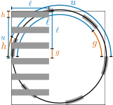
(a) $d=1$

(b) $d=2$

Figure 1: Illustration of the gray shaded boxes $B_{i}$ on the 1 and 2-dimensional torus.

In the following we first give a parameterized definition of the regions $B_{i}$ and then show how to choose the parameters for the above strategy to work; also see Figure 1. Each $B_{i}$ is an axis-aligned box, i.e., the cross product of intervals. Let $g,h>0$ such that $1/(g+h)$ is an even number. Think of $h$ of as the height of each box and of $g$ as the gap between the boxes, yielding $2k=1/(g+h)$ boxes. Now we define $B_{i}=[(i-1)\cdot(g+h),(i-1)\cdot(g+h)+h]\times[0,\frac{1}{2}-g]^{d-1}$ for $i\in[2k]$. We call the resulting regions $B_{1},\dots,B_{2k}$ the evenly spaced boxes of height $h$ and gap $g$. As before, $B_{i}$ and $B_{i+k}$ for $i\in[k]$ are opposite boxes.

With this, note that the distance between any pair of points in opposite boxes is at least $u=\frac{1}{2}-h$ (recall that we assume the infinity norm). Moreover, the distance between any pair of points in non-opposite regions is at most $\ell=\frac{1}{2}-g$. This yields the following lemma.

Lemma 3.1.

Let $B_{1},\dots,B_{2k}$ be evenly spaced boxes of height $h$ and gap $g$ in $\mathbb{T}^{d}$. Let $w_{\ell}=(\frac{1}{2}-g)^{d/2}\sqrt{\mu n}$ and $w_{u}=(\frac{1}{2}-h)^{d/2}\sqrt{\mu n}$. If we place one vertex of weight in $[w_{\ell},w_{u})$ in each box $B_{i}$, then these vertices form a co-matching.

Proof.

As observed above, the vertices in opposite boxes have distance at least $u=\frac{1}{2}-h$. Moreover, the vertices considered here have weight less than $w_{u}=u^{d/2}\sqrt{\mu n}$. As $w_{u}^{2}/(\mu nu^{d})=1$, these vertices are not connected (see Equation (6)). Similarly, vertices in non-opposite boxes have distance at most $\ell=\frac{1}{2}-g$ and weight at least $w_{\ell}=\ell^{d/2}\sqrt{\mu n}$. As $w_{\ell}^{2}/(\mu n\ell^{d})=1$, such vertices are connected. Hence, we get a co-matching. ∎

It now remains to choose $g$ and $h$ appropriately. First observe that, for the weight range in Lemma 3.1 to be non-empty, we need $w_{\ell}<w_{u}$ and thus $g>h$. Beyond that, we want to achieve the following three goals. First, the weight range needs to be sufficiently large such that we actually have a sufficient number of vertices in this range. For this, we want to choose $g$ substantially larger than $h$. Secondly, we want to make each box $B_{i}$ sufficiently large for it to contain a vertex with high probability. For this, we mainly want $h$ to be large. Thirdly, we want the number of boxes $2k=1/(g+h)$ to be large to obtain a large co-matching. For this, we want $g$ and $h$ to be small.

Note that these desires of choosing $h$ large, $g$ larger than $h$, and $g+h$ small are obviously conflicting. In the following, we show how to balance these goals out to obtain a co-matching of polynomial size. We start by estimating the number of vertices in the given weight range in the following lemma, which is slightly more general then we need.

Lemma 3.2.

Let $a,b>0$ be constants and let $g,h$ be functions of $n$ such that $g,h\in o(1)$. Let $S$ be the set of vertices with weight in $[(a-g)^{b}\sqrt{\mu n},(a-h)^{b}\sqrt{\mu n}]$. Then

$$\mathbb{E}\left[|S|\right]=n^{\frac{3-\tau}{2}}\cdot\mu^{\frac{1-\tau}{2}}ba^{b(1-\tau)-1}\cdot(g-h\pm O(g^{2}+h^{2})).$$ (7)

Proof.

Recall from (4) that the cumulative distribution function for the weights is $F(x)=1-x^{1-\tau}$. Thus, we get

$$\mathbb{E}\left[|S|\right] =n\cdot\left(F\left((a-h)^{b}\sqrt{\mu n}\right)-F\left((a-g)^{b}\sqrt{\mu n}\right)\right)$$

$$=n\cdot\left(((a-g)^{b}\sqrt{\mu n})^{1-\tau}-((a-h)^{b}\sqrt{\mu n})^{1-\tau}\right)$$

$$=\mu^{\frac{1-\tau}{2}}n^{\frac{3-\tau}{2}}\left((a-g)^{b(1-\tau)}-(a-h)^{b(1-\tau)}\right).$$ (8)

We can now use the Taylor expansion of $f(x)=(a-x)^{c}$ at $0$ to obtain the bound $f(x)=a^{c}-ca^{c-1}x\pm O(x^{2})$, which is valid for $x\in o(1)$. Since $g,h\in o(1)$ we can thus bound the above term in parentheses for $c=b(1-\tau)$ as

$$(a-g)^{c}-(a-h)^{c} =-ca^{c-1}g+ca^{c-1}h\pm O(g^{2}+h^{2})$$

$$=-ca^{c-1}(g-h\pm O(g^{2}+h^{2}))$$

$$=b(\tau-1)a^{b(1-\tau)-1}(g-h\pm O(g^{2}+h^{2})).$$ (9)

Equations (8) and (9) together yield the claim. ∎

Note that, if additionally $h\in o(g)$, we can write the last factor as $g(1-h/g\pm O(g+h^{2}/g))=g(1-o(1)\pm o(1))$ and obtain the following corollary.

Corollary 3.3.

Let $a,b>0$ be constants and let $g,h$ be functions of $n$ such that $g\in o(1)$ and $h\in o(g)$. Let $S$ be the set of vertices with weight in $[(a-g)^{b}\sqrt{\mu n},(a-h)^{b}\sqrt{\mu n}]$. Then

$$\mathbb{E}\left[|S|\right]=gn^{\frac{3-\tau}{2}}\cdot\mu^{\frac{1-\tau}{2}}ba^{b(1-\tau)-1}\cdot(1\pm o(1)).$$ (10)

Consider again the weights $w_{\ell}$ and $w_{u}$ as given in Lemma 3.1 and let $S$ be the set of vertices in $[w_{\ell},w_{u})$. Then Corollary 3.3 in particular implies that $S$ contains $\Theta(g\cdot n^{\frac{3-\tau}{2}})$ vertices in expectation.

With this, we turn to our second goal mentioned above, namely that each box $B_{i}$ should be sufficiently large.

Lemma 3.4.

Let $B_{1},\dots,B_{2k}$ be evenly spaced boxes of height $h$ and gap $g$ in $\mathbb{T}^{d}$. If $g\in o(1)$ then each box $B_{i}$ has volume $h/2^{d-1}\cdot(1-o(1))$.

Proof.

Recall that the height of $B_{i}$ is $h$ while its extent in all other dimensions is $\ell=\frac{1}{2}-g$. Thus its volume is $h\cdot(\frac{1}{2}-g)^{d-1}=h/2^{d-1}\cdot(1-2g)^{d-1}$. The claim follows from the fact that $(1-2g)^{d-1}$ approaches $1$ from below for $n\to\infty$ as $g\in o(1)$ and $d$ constant. ∎

Corollary 3.3 and Lemma 3.4 together tell us that the expected number of vertices in each box that have a weight in the desired range is in $\Theta(h\cdot g\cdot n^{\frac{3-\tau}{2}})$. Recall we want to choose $h$ and $g$ as small as possible such that each box still contains a vertex with high probability. We set $h=c\cdot n^{-\frac{3-\tau}{4}}$ and $g=c\cdot n^{-\frac{3-\tau}{4}+\varepsilon}$ for arbitrary constants $c>0$ and $\varepsilon>0$. Note that this satisfies the condition $h\in o(g)$ of Corollary 3.3 and yields an expected number of $\Theta(n^{\varepsilon})$ vertices with the desired weight in each box. Since the number of vertices in a given box follows a binomial distribution and since $\Theta(n^{\varepsilon})=\omega(\log(n))$, we can apply a Chernoff bound to conclude that actual number of vertices matches the expected value (up to constant factors) with probability $1-O(n^{-c^{\prime}})$ for any $c^{\prime}>0$ [1, Corollaries 2.3 and 2.4]. Together with a union bound, it follows that every box contains $\Theta(n^{\varepsilon})$ vertices (and thus at least one vertex) with probability $1-O(2k\cdot n^{-c^{\prime}})$. By choosing $g,h$, and $k$ appropriately, we obtain the following theorem.

Theorem 3.5.

Let $G$ be a $d$-dimensional GIRG with $T=0$, and let $s>0$ and $\varepsilon>0$ be arbitrary constants. Then, with high probability, $G$ contains a co-matching of size $s\cdot n^{\frac{3-\tau}{4}-\varepsilon}$ as induced subgraph.

Proof.

Let $B_{1},\dots,B_{2k}$ be evenly spaced boxes of height $h=c\cdot n^{-\frac{3-\tau}{4}}$ and gap $g=c\cdot n^{-\frac{3-\tau}{4}+\varepsilon}$ (for appropriately chosen $c>0$, which will be determined later). Let $w_{\ell}$ and $w_{u}$ be defined as in Lemma 3.1. As argued above, Corollary 3.3 and Lemma 3.4 imply that, with high probability, each box $B_{i}$ includes at least one vertex with weight in $[w_{\ell},w_{u})$. Thus, by Lemma 3.1 these $2k$ vertices form a co-matching.

Recall that $2k=1/(g+h)$. Thus, we can choose $c$ such that $2k=s\cdot n^{\frac{3-\tau}{4}-\varepsilon}$. Again, by the above argumentation, it follows that every box contains at least one vertex with probability $1-O(2kn^{-c^{\prime}})=1-O(n^{\frac{3-\tau}{4}-\varepsilon-c^{\prime}})$ for any constant $c^{\prime}>0$. Choosing $c^{\prime}$ sufficiently large then yields the claim. ∎

This theorem together with Lemma 2.2 directly imply the following corollary.

Corollary 3.6.

Let $G$ be a $d$-dimensional GIRG with $T=0$, and let $b>0$ and $\varepsilon>0$ be arbitrary constants. Then, with high probability, the number of maximal cliques in $G$ is at least $b^{n^{(3-\tau)/4-\varepsilon}}$.

Figure 2(a) shows this lower bound for $b=2$ against $n$. Interestingly, while Corollary 3.6 shows that the number of maximal cliques grows super-polynomially in $n$, for $\tau\gg 2$, this growth may still be slower than the linear slope $n$ for large geometric networks. This is of particular importance as the smaller order terms of the number of maximal cliques contain terms of at least $\Theta(n)$. Indeed, the number of maximal 2-cliques is lower bounded by the number of vertices of degree 1, which scales linearly by Equation (4). Thus, for practical purposes, the dominant term could be the linear term instead of the super-polynomial term, especially when the degree exponent is close to 3.

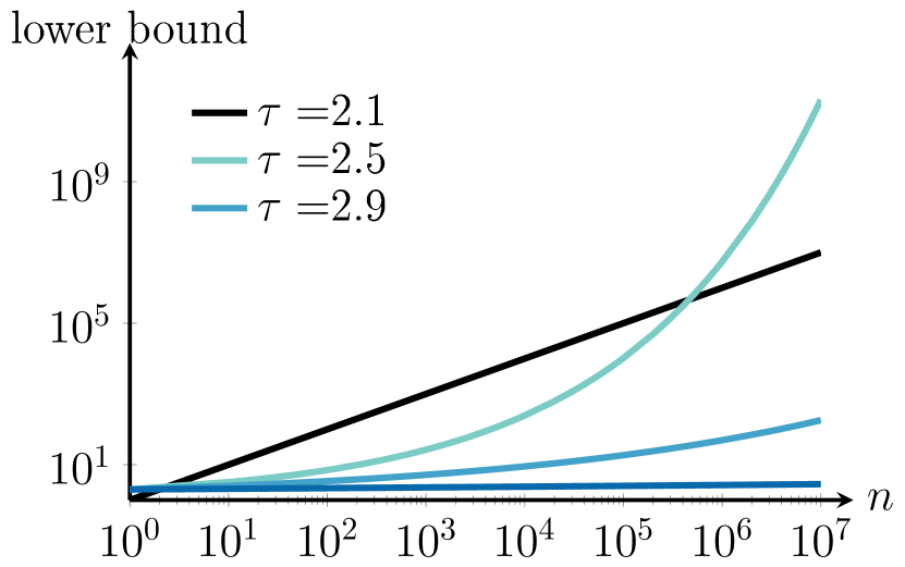
(a) GIRG lower bound

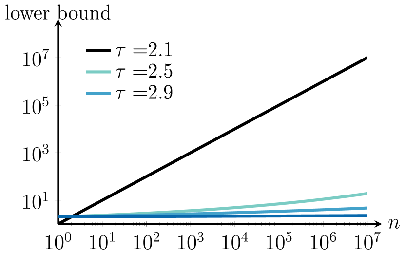
(b) GIRG lower bound, no torus

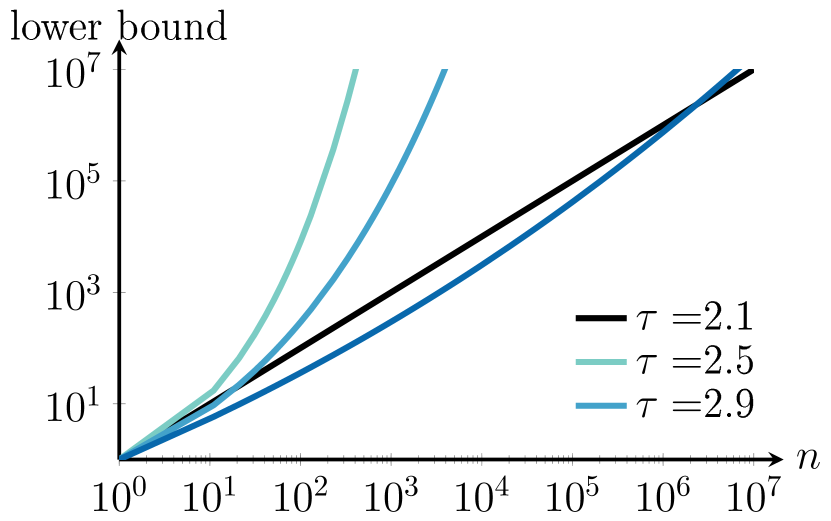
(c) IRG lower bound

Figure 2: Lower bound on the number of maximal cliques of Theorems 3.5 (with $b=2$),  3.7 (for $\varepsilon\downarrow 0$),  4.1 (for $\varepsilon\downarrow 0$) against $n$ for different values of $\tau$. The black line is the line $n$.

3.2 GIRG with 2-Dimensional Square

Our previous lower bound for the number of maximal cliques relies on the toroidal structure of the underlying space. We now show that even when the vertex positions are constrained to be positioned in the square $[0,1]^{2}$ instead, the GIRG still contains a super-polynomial number of maximal cliques.

Theorem 3.7.

For any $\varepsilon>0$ and $b>0$, a 2-dimensional GIRG with vertex positions uniformly distributed over $[0,1]^{2}$ equipped with the 2-norm and $T=0$ contains with high probability at least

$$Cb^{n^{\frac{3-\tau}{10}-\varepsilon}}$$ (11)

maximal cliques for some $C>0$.

(a) A circle of radius $R$ with several orange areas of height $h$.

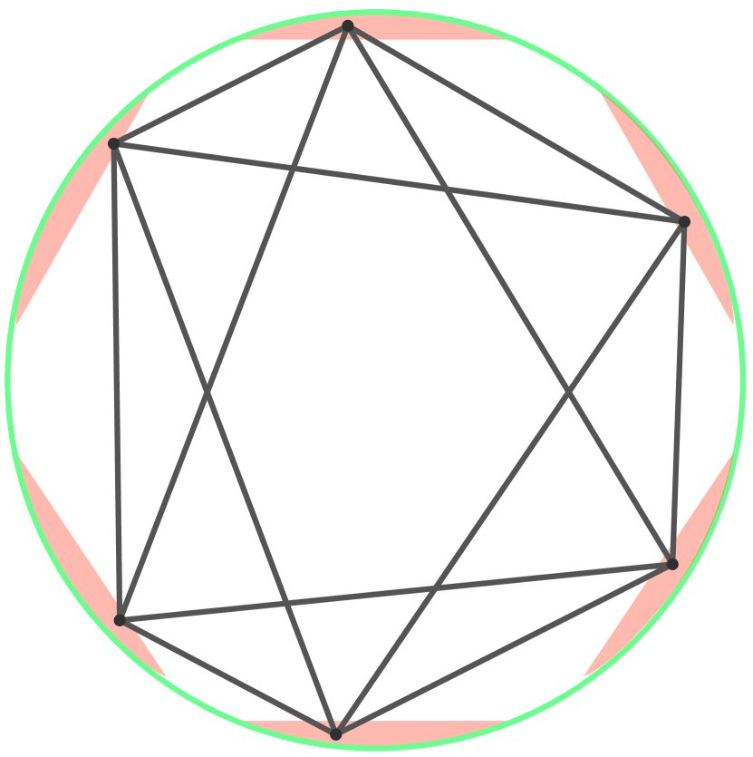
(b) Any set of vertices with one in each orange area form a clique minus a matching.

Figure 3: Clique minus a matching in the 2-dimensional GIRG.

Proof.

Let $S$ be the set of vertices with weights within $[a\sqrt{\mu n(1-c\cdot n^{-\beta})},a\sqrt{\mu n}]$ for some $0<a<1/4$ (and appropriately chosen $c>0$, which will be determined later). By Corollary 3.3,

$$\mathbb{E}\left[|S|\right]=n^{(3-\tau)/2-\beta}(1+o(1))$$ (12)

Let $\mathcal{C}$ be a circle on $[0,1]^{2}$ of constant radius $R<1/4$. We now create an even number of areas $B_{1},\dots,B_{2k}$ of height $h$, evenly distributed over $\mathcal{C}$ as illustrated in Figure 3(a). We ensure that any pair of vertices in two opposite areas $B_{i}$ and $B_{i+k}$ are disconnected. That is, the distance $t$ between the two ends of these areas should equal

$$t=a.$$ (13)

We also ensure that any pair of vertices in non-opposite areas connect. This means that the distance $l$ between the rightmost part of $B_{i}$ and the leftmost part of any non-opposite $B_{j}$ is at most

$$l=a\sqrt{1-c\cdot n^{-\beta}}.$$ (14)

The width $q$ of one of the $B_{i}$’s is given by

$$\frac{q}{2}=\sqrt{R^{2}-(R-h)^{2}}=\sqrt{h(2R-h)}=\sqrt{h(h+t)}=\sqrt{h(h+a)}.$$ (15)

Thus, the area of $B_{i}$ is given by

$$c_{1}h^{3/2}\sqrt{h+a},$$ (16)

for some constant $c_{1}>0$. The probability that a given area contains no vertices from $S$ is given by

$$\Big{(}1-c_{1}h^{3/2}\sqrt{h+a}\Big{)}^{|S|}\sim\exp(-c_{2}n^{(3-\tau)/2-\beta}h^{3/2}),$$ (17)

for some $c_{2}>0$.

We now calculate the maximal number of areas that we can pack on $\mathcal{C}$. The circumference of $\mathcal{C}$ is $2\pi R$. The arc length of a single area is at most $q\pi/2$. Furthermore, the arc length of the section with a chord of length $l$, $a(l)$, is given by

$$a(l)=2R\sin^{-1}(l/(2R)) =2R\sin^{-1}\Big{(}\frac{a\sqrt{1-c\cdot n^{-\beta}}}{a+2h}\Big{)}$$

$$=2R\sin^{-1}\Big{(}1-\frac{a+2h-a\sqrt{1-c\cdot n^{-\beta}}}{a+2h}\Big{)}$$

$$=\pi R-2^{3/2}R\sqrt{\frac{a+2h-a\sqrt{1-c\cdot n^{-\beta}}}{a+2h}}(1+o(1)),$$ (18)

using the Taylor series of $\sin^{-1}(1-x)$ around $x=0$. Now take $h=c\cdot n^{-\gamma}$. Then, by (3.2), $a(l)$ scales as

$$a(l)=\pi R-R\Theta\Big{(}\sqrt{(1-\sqrt{1-c\cdot n^{-\beta}})+c\cdot n^{-\gamma}}\Big{)}=\pi R-R\Theta(\sqrt{c\cdot n^{-\beta}+c\cdot n^{-\gamma}}).$$ (19)

Now the arc length between two adjacent sections $B_{i}$ and $B_{i+1}$ is equal to $\pi R-a(l)$. This means that the arc length between $B_{i}$ and $B_{i+1}$ scales as $\pi R-(\pi R-R\Theta\sqrt{c\cdot n^{-\beta}+c\cdot n^{-\gamma})})=R\Theta(\sqrt{c\cdot n^{-\beta}+c\cdot n^{-\gamma}})$.

The maximal value of the number of possible areas $2k$, is the total circumference of $\mathcal{C}$ divided by the arc length of an interval $B_{i}$ and the arc length between $B_{i}$ and $B_{i+1}$, which yields

$$2k=\frac{2\pi R}{R\Theta(\sqrt{c\cdot n^{-\beta}+c\cdot n^{-\gamma}})+\sqrt{h(h+a)}}=\Theta\Big{(}\min(n^{\beta/2},n^{\gamma/2})\Big{)}.$$ (20)

Thus, by choosing $c$ correctly, we can let $2k=s\cdot\min(n^{\beta/2},n^{\gamma/2})$ for any $s>0$. When all $i\in[2k]$ contain at least one vertex in $S$, any set of $2k$ vertices with exactly one vertex in each $B_{i}$ forms a clique minus a matching, as illustrated in Figure 3(b). Furthermore (17) shows that with high probability, all $B_{i}$ are non-empty, as long as $n^{(3-\tau)/2-\beta}h^{3/2}\to\infty$ as $n\to\infty$.

We therefore choose $\beta=(3-\tau)/5-\varepsilon$ and $\gamma=(3-\tau)/5$. Then, with high probability there is a clique minus a matching of size $2k=s\cdot n^{(3-\tau)/10-\varepsilon}$. Thus, by Lemma 2.2 and choosing $s$ sufficiently large yields that for fixed $b>0$ the number of maximal cliques can be bounded from below by

$$b^{n^{(3-\tau)/10-\varepsilon}}$$ (21)

∎

Figure 2(b) shows the lower bound of Theorem 3.7 against $n$. As for the toroidal case, the super-polynomial growth may be dominated by lower-order linear terms.

3.3 Non-Threshold Case

We now show how our constructions extend to the non-threshold GIRG, where the connection probability is given by Equation (5) instead of Equation (6).

Theorem 3.8.

Let $G$ be a $d$-dimensional GIRG with $T>0$, and let $s>0$ be an arbitrary constant. Then, there exists an $\varepsilon>0$ such that, with high probability, $G$ contains a co-matching of size $s\cdot n^{(3-\tau)/5}\cdot(\varepsilon\log n)^{-(1/2)}$ as induced subgraph.

Proof.

As before, we consider $2k$ boxes $B_{1},\ldots,B_{2k}$ with height $h$ and gap $g$, though now we choose

$$g=h\cdot(\varepsilon\log n)^{1/2}\qquad\text{and}\qquad h=\frac{1}{2s}\cdot n^{-\frac{3-\tau}{5}},$$

for a constant $\varepsilon>0$, which we determine below. We again focus on the vertex set $S$ containing all vertices with weights in $[w_{\ell},w_{u}]$, though our choice for $w_{u}$ is slightly different. In particular, we choose

$$w_{\ell}=(1/2-g)^{d/2}\sqrt{\mu n}\qquad\text{and}\qquad w_{u}=(1/2-(T/d+1)h)^{d/2}\sqrt{\mu n}.$$

Our goal now is to show that, with high probability, there exists at least one co-matching that contains one vertex from each box. That is, if $M$ denotes the number of such co-matchings, we want to show that $M>0$ with high probability.

We start by bounding the number the number of vertices from $S$ that lie in a given box $B_{i}$, denoted by $S(B_{i})$. Since $T$ and $d$ are constants and $(\varepsilon\log n)^{1/2}\in\omega(1)$, we have $(T/d+1)h\in o(g)$, allowing us to bound $\mathbb{E}[|S|]$ using Corollary 3.3, which yields

$$\mathbb{E}[|S|]=\Theta\left(gn^{\frac{3-\tau}{2}}\right).$$

Moreover, since the vertices are distributed uniformly at random in the ground space, the fraction of vertices from $S$ that lie in the box $B_{i}$ is proportional to its volume, which is $\Theta(h)$ according to Lemma 3.4. It follows that

$$\mathbb{E}[|S(B_{i})|]=\Theta\left(ghn^{\frac{3-\tau}{2}}\right)=\Theta\left(h^{2}n^{\frac{3-\tau}{2}}(\varepsilon\log n)^{1/2}\right)=\Theta\left(n^{(3-\tau)(1/2-2/5)}(\varepsilon\log n)^{1/2}\right).$$

Analogous to the proof of Lemma 3.4 we can apply a Chernoff bound to conclude that the number of vertices in $S(B_{i})$ matches the expected value (up to constant factors) with probability $1-O(n^{-c})$ for any $c>0$. Note that the number of boxes is given by

$$2k=\frac{1}{g+h}=\frac{1}{h((\varepsilon\log n)^{1/2}+1)}=\frac{2s\cdot n^{\frac{3-\tau}{5}}}{(\varepsilon\log n)^{1/2}+1},$$ (22)

which is at most $n$. Thus, applying the union bound yields that with high probability every box contains $n^{\prime}=\Theta(n^{(3-\tau)(1/2-2/5)}(\varepsilon\log n)^{1/2})$ vertices. In the following, we implicitly condition on this event to happen. Now recall that a co-matching consisting of one vertex from each box forms if each vertex is adjacent to the vertices in all other boxes, except the vertex from the opposite box.

Despite the temperature, vertices in non-opposite boxes are still adjacent with probability $1$, since the weight of two such vertices $i$ and $j$ is at least $w_{\ell}$ and their distance is at most $\frac{1}{2}-g$ and, thus, according to Equation 5

$$p_{ij}=\min\left\{\left(\frac{w_{i}w_{j}}{n\mu||x_{i}-x_{j}||^{d}}\right)^{1/T},1\right\}\geq\min\left\{\left(\frac{w_{\ell}^{2}}{n\mu(1/2-g)^{d}}\right)^{1/T},1\right\}=1.$$

In contrast to the threshold case, however, the probability for vertices in opposite boxes to be adjacent is no longer $0$. Since two such vertices $i$ and $j$ have distance at least $\frac{1}{2}-h$ and weight at most $w_{u}=(\frac{1}{2}-(T/d+1)h)^{d/2}\sqrt{\mu n}$, we can bound the probability for them to be adjacent using Equation 5, which yields

$$p_{ij} =\min\left\{\left(\frac{w_{i}w_{j}}{n\mu||x_{i}-x_{j}||^{d}}\right)^{1/T},1\right\}$$

$$\leq\min\left\{\left(\frac{w_{u}^{2}}{n\mu(\frac{1}{2}-h)^{d}}\right)^{1/T},1\right\}$$

$$=\min\left\{\left(\frac{1-(T/d+1)2h}{1-2h}\right)^{d/T},1\right\}$$

$$=\min\left\{\left(1-\frac{T}{d}\cdot\frac{2h}{1-2h}\right)^{d/T},1\right\}$$

$$\leq\min\left\{\left(1-\frac{T}{d}\cdot 2h\right)^{d/T},1\right\}.$$

Since $1-x\leq e^{-x}$, we obtain $p_{ij}\leq e^{-2h}$.

With this we are now ready to bound the probability $\mathbb{P}[M>0]$, that at least one co-matching forms that contains one vertex from each box. To this end, we need to find one non-edge in each pair of opposite boxes, i.e., each such pair needs to contain two vertices (one from each box) that are not adjacent. Conversely, the only way to not find a co-matching is if there exists one pair of opposite boxes such that all vertices in one box are adjacent to all vertices in the other. This happens with probability at most $(p_{ij})^{(n^{\prime})^{2}}$. Since there are $k$ pairs of opposite boxes, applying the union bound yields

$$\mathbb{P}[M=0]\leq k(p_{ij})^{(n^{\prime})^{2}}\leq k\exp(-2h(n^{\prime})^{2}).$$ (23)

Now recall that $n^{\prime}=\Theta(n^{(3-\tau)(1/2-2/5)}(\varepsilon\log n)^{1/2})$ and that $h=1/(2s)\cdot n^{-(3-\tau)/5}$. Consequently, we obtain

$$\mathbb{P}[M=0] \leq k\exp\left(-\Theta\left(n^{-(3-\tau)/5}\cdot n^{(3-\tau)(1-4/5)}\cdot\varepsilon\log n\right)\right)$$

$$=k\exp\left(-\Theta(\varepsilon\log n)\right)$$

$$=kn^{-\Theta(\varepsilon)}.$$

Moreover, since $k=O(n^{(3-\tau)/5})$ (see Equation 22), we have

$$\mathbb{P}[M=0]=O\left(n^{(3-\tau)/5-\Theta(\varepsilon)}\right),$$

meaning, for sufficiently large $n$, we can choose $\varepsilon$ such that $\mathbb{P}[M=0]=O(n^{-1})$ and, conversely, $\mathbb{P}[M>0]=1-O(n^{-1})$. So with high probability there exists at least one co-matching of size

$$2k=\frac{2s\cdot n^{\frac{3-\tau}{5}}}{(\varepsilon\log n)^{1/2}+1}\geq\frac{2s\cdot n^{\frac{3-\tau}{5}}}{2(\varepsilon\log n)^{1/2}}=\frac{s\cdot n^{\frac{3-\tau}{5}}}{(\varepsilon\log n)^{1/2}},$$

where the inequality holds for sufficiently large $n$. ∎

Together with Lemma 2.2 we obtain the following corollary.

Corollary 3.9.

Let $G$ be a $d$-dimensional GIRG with $T>0$, and let $b>0$ be an arbitrary constant. Then there exists an $\varepsilon>0$ such that, with high probability, the number of maximal cliques in $G$ is at least $b^{n^{(3-\tau)/5}\cdot(\varepsilon\log n)^{-(1/2)}}$.

We can extend Theorem 3.7 to non-zero temperature in a very similar fashion (proof is in Appendix A)

Theorem 3.10.

For any $\varepsilon>0$ and $b>1$, a 2-dimensional GIRG with $T>0$ and vertex positions uniformly distributed over $[0,1]^{2}$ contains with high probability at least

$$b^{n^{\frac{3-\tau}{12}-\varepsilon}\log(n)^{1-\varepsilon}}.$$ (24)

maximal cliques.

4 Inhomogeneous Random Graphs (IRG)

We now turn to a random graph model that is scale-free, but does not contain a source of geometry, the inhomogeneous random graph (IRG). We show that also in this model, the number of maximal cliques scales super-polynomially in the network size $n$. In the IRG, the probability that two vertices of weights $w_{u}$ and $w_{v}$ connect is independently given by

$$p(w_{u},w_{v})=\min\Big{(}\frac{w_{u}w_{v}}{\mu n},1\Big{)},$$ (25)

where $\mu$ controls the expected average degree. Furthermore, as done above, we assume that the weights are independently drawn from the power-law distribution; see Equation (4).

To show a lower bound on the number of maximal cliques, we make use of the fact that an IRG contains a not too small rather dense subgraph with high probability. The following theorem is obtained by looking just at the subgraph induced by vertices with weights in a certain range. We chose the specific range to satisfy three criteria. First, the range is sufficiently large, such that the subgraph contains many vertices. Second, the range is sufficiently small such that all vertex pairs in the subgraph are connected with a similar probability. And third, the weights are large enough such that a densely connected subgraph forms, but not so large that the vertices merge into a single clique.

Theorem 4.1.

Let $G$ be an IRG with $\tau\in(2,3)$ and let $b>1$ and $\varepsilon\in(0,\frac{3-\tau}{4})$ be arbitrary constants. Then, the expected number of maximal cliques in $G$ is in $\Omega\big{(}b^{n^{(3-\tau)/4-\varepsilon}\log n}\big{)}$.

Proof.

We show that already the subgraph $G^{\prime}$ induced by the vertices in a certain weigh range has the claimed expected number of cliques. To define $G^{\prime}$, we consider weights in $[w_{\ell},w_{u}]$ with $w_{\ell}=\sqrt{(1-g)\mu n}$ and $w_{u}=\sqrt{(1-h)\mu n}$. To abbreviate notation, let

$$\gamma=n^{\frac{3-\tau}{4}}.$$

For constants $a$ and $c$ we determine later, we choose $g$ and $h$ as

$$g=ah\quad\text{and}\quad h=cn^{\varepsilon}\log(n)\gamma^{-1}.$$

Note that $w_{\ell}<w_{u}$ if and only if $a>1$. Let $n^{\prime}$ be the number of vertices in $G^{\prime}$. From Lemma 3.2 it follows

$$\mathbb{E}\left[n^{\prime}\right]\in\Theta(\gamma^{2}\cdot n^{\varepsilon}\log(n)\gamma^{-1})=\Theta(n^{\varepsilon}\gamma\log n).$$

As every vertex has independently the same probability to be in $G^{\prime}$, a Chernoff bound implies that $n^{\prime}\in\Theta(n^{\varepsilon}\gamma\log n)$ holds with high probability. Thus, in the following, we implicitly condition on this event to happen.

To give a lower bound on the number of maximal cliques in $G^{\prime}$, we only count the number $N_{k}$ of maximal cliques of size $k$ with

$$k=\frac{3\varepsilon}{c}n^{-\varepsilon}\gamma.$$

We note that this is the same constant $c$ as in the definition of $h$ above. To compute the expectation for the number $N_{k}$ of maximal cliques, we consider all vertex sets of size $k$ of the vertices in $G^{\prime}$, i.e., for a fixed subset $C$ of size $k$, we obtain

$$\mathbb{E}\left[N_{k}\right]\geq{n^{\prime}\choose k}\mathbb{P}\left(C\text{ is a clique}\right)\mathbb{P}\left(C\text{ maximal}\mid C\text{ is a clique.}\right).$$

In the following, we give estimates for the three terms individually.

We start with the event that $C$ is a clique. Due to the lower and upper bound on the weights in $G^{\prime}$, it follows that any pair of vertices in $G^{\prime}$ is connected with probability at least $p_{\ell}=1-g$ and at most $p_{u}=1-h$. Thus, for a fixed subset $C$ of vertices of size $|C|=k$, the probability that all $k$ vertices are pairwise connected is at least $p_{\ell}^{k(k-1)/2}=(1-g)^{k(k-1)/2}$. As $g$ goes to $0$ for growing $n$ and $1-x\in\Omega(\exp(-x))$ in this case, we get

$$\mathbb{P}\left(C\text{ is a clique}\right)\geq(1-g)^{k(k-1)/2}\in\Omega\left(\exp\left(-\frac{gk(k-1)}{2}\right)\right).$$ (26)

For $C$ to be a maximal clique (conditioning on it being a clique), additionally no other vertex can be connected to all vertices from $C$. This probability is at least $(1-p_{u}^{k})^{n^{\prime}-k}=(1-(1-h)^{k})^{n^{\prime}-k}$. As $1-x\leq\exp(-x)$, it follows that $(1-h)^{k}\leq\exp(-hk)=n^{-3\varepsilon}$, where the last equality follows from plugging in the values we chose for $h$ and $k$. Again using $1-x\in\Omega(\exp(-x))$ for sufficiently small $x$, we can conclude that

$$\mathbb{P}\left(C\text{ maximal}\mid C\text{ is a clique}\right) \geq(1-(1-h)^{k})^{n^{\prime}-k}$$

$$\geq(1-n^{-3\varepsilon})^{n^{\prime}-k}$$ (27)

$$\in\Omega\Big{(}\exp\big{(}-n^{-3\varepsilon}(n^{\prime}-k)\big{)}\Big{)}.$$

Finally, for the binomial coefficient, we get

$${n^{\prime}\choose k}\geq\left(\frac{n^{\prime}}{k}\right)^{k}=\exp\left(\log\left(\frac{n^{\prime}}{k}\right)k\right).$$ (28)

Combining Equations (26), (27), and (28), it remains to show that for every constant $b>1$, we can choose the constants $a>1$ and $c$ in the definitions of $g$ and $h$ such that

$$\log\left(\frac{n^{\prime}}{k}\right)k-\frac{gk(k-1)}{2}-n^{-3\varepsilon}(n^{\prime}-k)\stackrel{{\scriptstyle\text{\tiny(to be shown)}}}{{>}}n^{-\varepsilon}\gamma\log n\log b=n^{\frac{3-\tau}{4}-\varepsilon}\log n\log b.$$

This can be achieved by simply plugging in the values for $n^{\prime}$, $k$, and $g$. For the first (and only positive) term, we obtain

$$\log\left(\frac{n^{\prime}}{k}\right)k =\log\left(\frac{\Theta(n^{\varepsilon}\log(n)\gamma)}{3\varepsilon/cn^{-\varepsilon}\gamma}\right)\frac{3\varepsilon}{c}n^{-\varepsilon}\gamma$$

$$=\log\left(n^{2\varepsilon}\Theta(\log n)\right)\frac{3\varepsilon}{c}n^{-\varepsilon}\gamma$$

and thus for sufficiently large $$n$$

$$\geq\frac{6\varepsilon^{2}}{c}n^{-\varepsilon}\gamma\log n.$$

For the negative terms, we start with the latter and obtain

$$n^{-3\varepsilon}(n^{\prime}-k)\in\Theta(n^{-3\varepsilon}n^{\varepsilon}\gamma\log n)=\Theta(n^{-2\varepsilon}\gamma\log n).$$

This is asymptotically smaller than the positive term and can thus be ignored.

For the other negative term, first note that $gk=3a\varepsilon\log n$. Thus, we obtain

$$\frac{gk(k-1)}{2}\leq\frac{3a\varepsilon}{2}\log(n)k=\frac{3a\varepsilon}{2}\log(n)\frac{3\varepsilon}{c}n^{-\varepsilon}\gamma=\frac{9a\varepsilon^{2}}{2c}n^{-\varepsilon}\gamma\log n.$$

Together with the positive term, we obtain that for sufficiently large $n$, it holds

$$\log\left(\frac{n^{\prime}}{k}\right)k-\frac{gk(k-1)}{2} \geq\frac{6\varepsilon^{2}}{c}n^{-\varepsilon}\gamma\log n-\frac{9a\varepsilon^{2}}{2c}n^{-\varepsilon}\gamma\log n$$

$$=\left(6-\frac{9a}{2}\right)\frac{\varepsilon^{2}}{c}n^{-\varepsilon}\gamma\log n.$$

With this, we can choose $a>1$ such that the first factor is positive and we can choose $c$ such that $\varepsilon^{2}/c=\log b$, which proves the claim. ∎

Figure 2(c) shows that the lower bound provided by Theorem 4.1 may still be smaller than linear for networks that are quite large, especially when $\tau\approx 3$.

4.1 Small Maximal Cliques are Rare

We now focus on the maximal cliques of a fixed size in the IRG. How many maximal cliques of size $k$ are present in an IRG?

Let $N(K_{k})$ denote the number of maximal cliques of size $k$. Furthermore, let $M_{n}(\varepsilon)$ denote

$$M_{n}(\varepsilon)=\{({v_{1},\ldots,v_{k}})\colon w_{i}\in[\varepsilon,1/\varepsilon](\mu n)^{\frac{\tau-2}{\tau-1}}\ \text{ for }i=1,2\text{ and }w_{i}\in[\varepsilon,1/\varepsilon](\mu n)^{\frac{1}{\tau-1}}\ \forall i\in\{3,\dots,k\}\}.$$ (29)

Thus, $M_{n}(\varepsilon)$ is the set of sets of $k$ vertices such that two vertices have weight approximately $n^{(\tau-2)/(\tau-1)}$, and all other vertices have weights approximately $n^{1/(\tau-1)}$. Denote the number of maximal $k$-cliques with sets of vertices in $M_{n}(\varepsilon)$ by $N(K_{k},M_{n}(\varepsilon))$. Then, the following theorem shows that these ‘typical’ maximal cliques are asymptotically all maximal cliques. Furthermore, it shows that all maximal cliques of size $k>2$ occur equally frequently in scaling, and they also appear on the same types of vertices. Here we use $\stackrel{{\scriptstyle\mathbb{P}}}{{\longrightarrow}}$ to denote convergence in probability.

Theorem 4.2 (Maximal clique localization).

For any fixed $k\geq 3$,

1. For any $\varepsilon_{n}$ such that $\lim_{n\to\infty}\varepsilon_{n}=0$,

   $$\frac{N\big{(}K_{k},M_{n}\left(\varepsilon_{n}\right)\big{)}}{N(K_{k})}\stackrel{{\scriptstyle\mathbb{P}}}{{\longrightarrow}}1.$$ (30)

2. Furthermore, for any fixed $0<\varepsilon<1$,

   $$\mathbb{E}\left[N(K_{k},M_{n}(\varepsilon))\right]=\Theta{n^{(3-\tau)(2\tau-3)/(\tau-1)}}.$$ (31)

Theorem 4.2(i) states that asymptotically all maximal $k$-cliques are formed between two vertices of weights proportional to $n^{(\tau-2)/(\tau-1)}$ and all other vertices of weights proportional to $n^{1/(\tau-1)}$. Theorem 4.2(ii) then shows that there are proportional to $n^{(3-\tau)(2\tau-3)/(\tau-1)}$ such maximal $k$-cliques. Note that this scaling is significantly smaller than the scaling of the total number of $k$-cliques, which scales as $n^{k/2(3-\tau)}$ [13]. Interestingly, the scaling of the number of max-cliques is $k$-independent, contrary to the total number of cliques. In particular, the number of $k$ maximal cliques is always $o(n)$, contrary to the number of $k$-cliques which scales larger than $n$ when $\tau<3-2/k$. This shows once more that the large number of maximal cliques in the IRG is caused by extremely large maximal cliques, as fixed-size maximal cliques are only linearly many.

To prove this theorem, we need the following technical lemma, which is proven in Appendix B:

Lemma 4.3.

$$\int_{0}^{1}\dots\int_{0}^{1}\int_{0}^{\infty}\int_{x_{1}}^{\infty}x_{1}^{k-1-\tau}x_{2}^{1-\tau}x_{3}^{1-\tau}\cdots x_{k}^{1-\tau}\prod_{i=3}^{k}\min\Big{(}x_{2}x_{i},1\Big{)}e^{-\mu^{1-\tau}x_{1}x_{2}^{\tau-2}}dx_{2}dx_{1}\dots dx_{k}<\infty$$ (32)

Furthermore, we need a lemma that bounds the probability that a given clique on vertices of weights $x_{1}\leq x_{2}\dots\leq x_{k}$ is maximal:

Lemma 4.4.

The probability that a given clique between $k$ vertices of weights $x_{1}\leq x_{2}\dots\leq x_{k}$ is maximal is bounded by

$$\exp\Big{(}-C_{1}n^{2-\tau}\mu^{1-\tau}x_{1}x_{2}^{\tau-2}\Big{)}(1+o(1))\leq\mathbb{P}\left(\text{clique on weights }x_{1},\dots,x_{k}\text{ maximal}\right)$$

$$\leq\exp\Big{(}-C_{2}n^{2-\tau}\mu^{1-\tau}x_{1}x_{2}^{\tau-2}\Big{)},$$ (33)

for some $0<C_{1}\leq C_{2}<\infty$.

Proof.

When $x_{1}\leq x_{2}\leq\dots\leq x_{k}$, we can compute the probability that this $k$ clique is part of a larger clique with a randomly chosen vertex as

$$\int_{1}^{\infty}w^{-\tau}\prod_{i\in[k]}\min\Big{(}\frac{wx_{i}}{\mu n},1\Big{)}dw$$

$$=\frac{x_{1}\dots x_{k}}{(\mu n)^{k}}\int_{1}^{\mu n/x_{k}}w^{k-\tau}dw+\frac{x_{1}\dots x_{{k-1}}}{(\mu n)^{k-1}}\int_{\mu n/x_{k}}^{\mu n/x_{{k-1}}}w^{k-1-\tau}dw$$

$$\quad+\dots+\frac{x_{1}x_{{2}}}{(\mu n)^{2}}\int_{\mu n/x_{3}}^{\mu n/x_{{2}}}w^{2-\tau}dw+\frac{x_{1}}{\mu n}\int_{\mu n/x_{2}}^{\mu n/x_{{1}}}w^{1-\tau}dw+\int_{\mu n/x_{1}}^{\infty}w^{-\tau}dw$$

$$=c_{k}\frac{x_{1}\dots x_{k}}{(\mu n)^{k}}\Big{(}\frac{\mu n}{x_{k}}\Big{)}^{k+1-\tau}+\dots+c_{2}\frac{x_{1}}{\mu n}\Big{(}\frac{\mu n}{x_{2}}\Big{)}^{2-\tau}+c_{1}\Big{(}\frac{\mu n}{x_{1}}\Big{)}^{1-\tau},$$ (34)

for some $c_{1},\dots,c_{k}>0.$ When $x_{1}\leq x_{2}\leq\dots\leq x_{k}$, this term becomes

$$(\mu n)^{1-\tau}\sum_{l=1}^{k}c_{l}x_{l}^{-l+\tau}\prod_{i<l}x_{i}.$$ (35)

The ratio between two consecutive terms of this summation equals

$$\frac{x_{l}^{\tau-l}x_{1}\dots x_{{l-1}}}{x_{{l+1}}^{\tau-l-1}x_{1}\dots x_{{l}}}=\Big{(}\frac{x_{l}}{x_{{l+1}}}\Big{)}^{\tau-l-1}.$$ (36)

Now as $x_{l}\leq x_{{l+1}}$ and $\tau\in(2,3)$, this ratio is larger than 1 for $l\geq 2$, and smaller than one for $l=1$. This means that the summation can be dominated by

$$(\mu n)^{1-\tau}\sum_{l=1}^{k}c_{l}x_{l}^{-l+\tau}\prod_{i<l}x_{i}\leq C(\mu n)^{1-\tau}x_{1}x_{2}^{\tau-2},$$ (37)

for some $C>0$.

Thus, the probability that a clique on vertices with weights $x_{1},\dots,x_{k}$ is maximal can be upper bounded by

$$\mathbb{P}\left((x_{1},\dots,x_{k})\text{ clique maximal }\right) \leq\Big{(}1-C(\mu n)^{1-\tau}x_{1}x_{2}^{\tau-2}\Big{)}^{n}$$

$$\leq\exp\Big{(}-Cn^{2-\tau}\mu^{1-\tau}x_{1}x_{2}^{\tau-2}\Big{)}.$$ (38)

We lower bound the probability that the clique is maximal by using that

$$(\mu n)^{1-\tau}\sum_{l=1}^{k}c_{l}x_{l}^{-l+\tau}\prod_{i<l}x_{i}\geq c_{2}(\mu n)^{1-\tau}x_{1}x_{2}^{\tau-2}.$$ (39)

Thus,

$$\mathbb{P}\left((x_{1},\dots,x_{k})\text{ clique maximal }\right) \geq\Big{(}1-c_{2}(\mu n)^{1-\tau}x_{1}x_{2}^{\tau-2}\Big{)}^{n}$$

$$\geq\exp\Big{(}-c_{2}n^{2-\tau}\mu^{1-\tau}x_{1}x_{2}^{\tau-2}/(1+c_{2}n^{1-\tau}\mu^{1-\tau}x_{1}x_{2}^{\tau-2})\Big{)}$$

$$=\exp\Big{(}-c_{2}n^{2-\tau}\mu^{1-\tau}x_{1}x_{2}^{\tau-2}\Big{)}(1+o(1)).$$ (40)

∎

Figure 4: Scaling of the number of maximal $k$-cliques, and the total number of (not necessarily maximal) 3,4,5-cliques.

Now we are ready to prove Theorem 4.2:

Proof of Theorem 4.2.

Fix $\ell_{i}\leq u_{i}$ for $i\in[k]$. We now compute the expected number of maximal $k$-cliques in which the vertices have weights $n^{(\tau-2)/(\tau-1)}[\ell_{i},u_{i}]$ for $i=1,2$, and $n^{1/(\tau-1)}[\ell_{i},u_{i}]$ for $i\geq 3$.

We bound the expected number of such maximal copies of $K_{k}$ by

$$\sum_{\bm{v}}\mathbb{E}\left[I(K_{k},\bm{v})\mathbbm{1}_{\left\{w_{v_{i}}\in[\ell_{i},u_{i}]n^{(\tau-2)/(\tau-1)},\ i=1,2,\ w_{v_{i}}\in[\ell_{i},u_{i}]n^{1/(\tau-1)},\ i\geq 3\right\}}\right]$$

$$=n^{k}\int_{\ell_{1}n^{(\tau-2)/(\tau-1)}}^{u_{1}n^{(\tau-2)/(\tau-1)}}\int_{\ell_{2}n^{(\tau-2)/(\tau-1)}}^{u_{2}n^{(\tau-2)/(\tau-1)}}\cdots\int_{\ell_{k}n^{1/(\tau-1)}}^{u_{k}n^{1/(\tau-1)}}(x_{1}\cdots x_{k})^{-\tau}\prod_{\mathclap{1\leq i<j\leq k}}\min\left(\frac{x_{i}x_{j}}{n},1\right)$$

$$\quad\cdot\mathbb{P}\left((x_{1},\dots,x_{k})\text{ clique maximal}\right){\rm d}x_{k}\cdots{\rm d}x_{1},$$

where $I(K_{k},\bm{v})$ is the indicator that a maximal $k$-clique is present on vertices $\bm{v}$, and the sum over $\bm{v}$ is over all possible sets of $k$ vertices. Now the probability that a clique is maximal can be upper bounded as in Lemma 4.4.

We bound the minimum in (4.1) by

• $x_{i}x_{j}/n$ for $\{i,j\}=\{1,2\}$ or $i=1,j\geq 3$;

• 1 for $i,j\geq 3$ .

Making the change of variables $x_{i}=y_{i}n^{1/(\tau-1)}$ for $i=3,\dots,k$ and $x_{i}=y_{i}/n^{(\tau-2)/(\tau-1)}$ otherwise, we obtain the bound

$$\sum_{\bm{v}}\mathbb{E}\left[I(K_{k},\bm{v})\mathbbm{1}_{\left\{w_{v_{i}}\in[\ell_{i},u_{i}]n^{(\tau-2)/(\tau-1)},\ i=1,2,\ w_{v_{i}}\in[\ell_{i},u_{i}]n^{1/(\tau-1)},\ i\geq 3\right\}}\right]$$

$$\leq\tilde{K}n^{k}n^{2(\tau-2)/(\tau-1)-k+1}$$

$$\times\int_{\ell_{1}}^{u_{1}}\int_{y_{1}}^{u_{2}}\int^{u_{3}}_{\ell_{3}}\cdots\int^{u_{k}}_{\ell_{k}}y_{1}^{2-\tau}y_{2}^{1-\tau}y_{3}^{1-\tau}\dots y_{k}^{1-\tau}\prod_{j\geq 3}\min(y_{2}y_{j},1)\exp(-\mu^{1-\tau}y_{1}y_{2}^{\tau-2}){\rm d}y_{k}\cdots{\rm d}y_{1},$$ (41)

for some $\tilde{K}>0$. Because the weights are sampled i.i.d. from a power-law distribution, the maximal weight $w_{\max}$ satisfies that for any $\eta_{n}\to 0$, $w_{\max}\leq n^{1/(\tau-1)}/\eta_{n}$ with high probability. Thus, we may assume that $u_{i}\leq 1/\eta_{n}$ when $i\geq 3$. Now suppose that at least one vertex has weight smaller than $\varepsilon_{n}n^{(\tau-2)/(\tau-1)}$ for $i=1,2$ or smaller than $\varepsilon_{n}n^{1/(\tau-1)}$ for $i\geq 3$. This corresponds to taking $u_{i}=\varepsilon_{n}$ and $\ell_{i}=0$ for at least one $i$, or at least one integral in (4.1) with interval $[0,\varepsilon_{n}]$. Similarly, when vertex 1 or 2 has weight higher than $1/\varepsilon_{n}n^{(\tau-2)/(\tau-1)}$, this corresponds to taking $\ell_{i}=1/\varepsilon_{n}$ and $u_{i}=\infty$ for $i=1$ or 2, or at least one integral in (4.1) with interval $[1/\varepsilon_{n},\infty]$. Lemma 4.3 then shows that these integrals tends to zero when choosing $u_{i}=\eta_{n}$ fixed for $i\geq 3$ and $\varepsilon_{n}\to 0$. Thus, choosing $\eta_{n}\to 0$ sufficiently slowly compared to $\varepsilon_{n}$ yields that

$$\sum_{\bm{v}}\mathbb{E}\left[I(K_{k},\bm{v})\mathbbm{1}_{\left\{\bm{v}\notin\Gamma_{n}(\varepsilon_{n},\eta_{n})\right\}}\right]=o((n^{(3-\tau)(2\tau-3)/(\tau-1)}),$$ (42)

where

$$\Gamma_{n}(\varepsilon_{n},\eta_{n})=\{(v_{1},\dots,v_{k})\colon w_{v_{i}}\in n^{(\tau-2)/(\tau-1)}[\varepsilon_{n},1/\varepsilon_{n}],i=1,2\ n^{1/(\tau-1)}[\varepsilon_{n},1/\eta_{n}]\}.$$ (43)

Let $\bar{\Gamma}_{n}(\varepsilon_{n},\eta_{n})$ be the complement of $\Gamma_{n}(\varepsilon_{n},\eta_{n})$. Denote the number of maximal cliques with vertices in $\bar{\Gamma}_{n}(\varepsilon_{n},\eta_{n})$ by $N(K_{k},\bar{\Gamma}_{n}(\varepsilon_{n},\eta_{n}))$. Since $w_{\max}\leq n^{1/(\tau-1)}/\eta_{n}$ with high probability, $\Gamma_{n}(\varepsilon_{n},\eta_{n})=M_{n}(\varepsilon_{n})$ with high probability. Therefore, with high probability,

$$N\Big{(}K_{k},\bar{M}_{n}\left(\varepsilon_{n}\right)\Big{)}=N\Big{(}K_{k},\bar{\Gamma}_{n}(\varepsilon_{n},\eta_{n})\Big{)},$$ (44)

where $N\Big{(}K_{k},\bar{M}_{n}\left(\varepsilon_{n}\right)\big{)}$ denotes the number of maximal $k$-cliques on vertices not in $M_{n}\left(\varepsilon_{n}\right)$. By (42) and the Markov inequality, we have for all $\epsilon>0$

$$\lim_{n\to\infty}\mathbb{P}\left(\left|\frac{N\Big{(}K_{k},\bar{\Gamma}_{n}(\varepsilon_{n},\eta_{n})\Big{)}}{n^{(3-\tau)(2\tau-3)/(\tau-1)}}\right|>\epsilon\right)=0.$$ (45)

Furthermore, Lemma 4.3 combined with the lower bound in (4.1) shows that when choosing $u_{i}=1/\varepsilon$ and $\ell_{i}=\varepsilon$ for some fixed $\varepsilon>0$ for all $i$,

$$\mathbb{E}\left[N(K_{k},M_{n}(\varepsilon))\right]=\Theta(n^{(3-\tau)(2\tau-3)/(\tau-1)}).$$ (46)

Thus, for fixed $\varepsilon>0$,

$$N(K_{k}) =N(K_{k},M_{n}(\varepsilon))+N(K_{k},\bar{M}_{n}(\varepsilon))=\Theta_{p}(n^{(3-\tau)(2\tau-3)/(\tau-1)}),$$ (47)

which shows that

$$\frac{N\Big{(}K_{k},M_{n}\left(\varepsilon_{n}\right)\big{)}}{N(K_{k})}\stackrel{{\scriptstyle\mathbb{P}}}{{\longrightarrow}}1,$$ (48)

as required. This completes the proof of Theorem 4.2. ∎

5 Experiments

As mentioned in the introduction, empirical evidence suggests that the number of maximal cliques in IRGs and GIRGs is small [3]. In fact, all generated networks with $n=$50\text{\,}\mathrm{k}$$ nodes and expected average degree $10$ have fewer maximal cliques than edges. This stands in stark contrast to our super-polynomial lower bounds. This discrepancy probably comes from the fact that $n=$50\text{\,}\mathrm{k}$$ is low enough that a linear lower-order term dominates the super-polynomial terms. In this section, we complement our theoretical lower bounds with experiments with an $n$ that is sufficiently large to make the super-polynomial terms dominant. Additionally, we ran some experiments on dense and super-dense Erdős–Rényi graphs.

5.1 Cliques in the Dense Subgraph of GIRGs and IRGs

Our theoretical lower bounds are based on the existence of a dense subgraph among the vertices with weights $\Theta(\sqrt{n})$. To experimentally observe the super-polynomial scaling, we generate IRGs and GIRGs restricted to vertices of high weight. This restriction lets us consider much larger values of $n$. In the following, we first describe the exact experiment setup, before describing and discussing the results.

Experiment Setup.

We generate IRGs and GIRGs with varying number of vertices $n$ and deterministic power-law weights where the $v$th vertex has weight

$$w_{v}=\left(\frac{n}{v}\right)^{\frac{1}{\tau-1}}.$$

Note that the minimum weight is $w_{n}=1$.

We use the power-law exponents $\tau\in\{2.2,2.5,2.8\}$ and for GIRGs we consider the temperatures $T\in\{0,0.4,0.8\}$ and dimension $d=1$. For each parameter setting, we consider two subgraphs: The subgraph induced vertices with $0.5\sqrt{n}\leq w_{i}\leq\sqrt{n}$ and with just $0.5\sqrt{n}\leq w_{i}\leq n$. In preliminary experiments, we also tried constant factors other than $0.5$, yielding comparable results.

As connection probability for the IRGs between the $u$th and $v$th vertex, we use $\min\{1,w_{u}w_{v}/n\}$, i.e., vertices of weight $1$ have connection probability $1/n$ and vertices of weight at least $\sqrt{n}$ are deterministically connected. For GIRGs, we choose the constant factor $\mu$ in Equation (5) such that we obtain the same expected average degree as for the corresponding IRG in the considered subgraph. For each of these configurations, we generate $10$ graphs. Figure 5 shows the average.

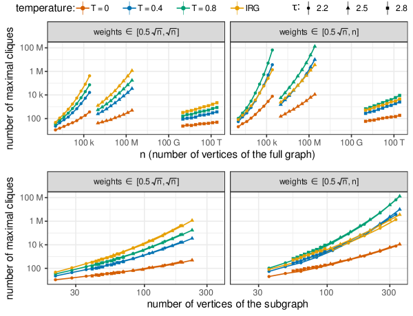
Figure 5: The number of maximal cliques of the dense subgraph of GIRGs and IRGs. The considered subgraphs contain all vertices with weights in $[0.5\sqrt{n},\sqrt{n}]$ (left column) and $[0.5\sqrt{n},n]$ (right column). The top and bottom plots show the number of cliques with respect to the size of the full graph, and with respect to the size of the considered subgraph, respectively. All axes are logarithmic. Each point is the average of $10$ sampled graphs.

General Observations.

One can clearly see in Figure 5 (top row) that the scaling of the number of cliques depending on the graph size is super-polynomial (upward curves in a plot with logarithmic axes). Thus, on the one hand, this agrees with our theoretical analysis. On the other hand, the plots also explain why previous experiments [3] showed a small number of cliques: While the scaling is super-polynomial, the constant factors are quite low. In the top-left plot for $\tau=2.5$, more than $200\text{\,}\mathrm{M}$ nodes are necessary to get just barely above $1\text{\,}\mathrm{M}$ maximal cliques in the dense subgraph. For $\tau=0.8$ this is even more extreme with $n=$200\text{\,}\mathrm{T}$$ yielding only $10\text{\,}\mathrm{k}$ maximal cliques. Thus, unless we deal with huge graphs, the maximal cliques in the dense part of the graph are dominated by the number of cliques in the sparser parts, despite the super-polynomial growth of the former.

Effect of the Power-Law Exponent $\tau$.

The top plots of Figure 5 show that a smaller power-law exponent $\tau$ leads to more maximal cliques. The bottom plots show the number of cliques with respect to the size of the dense subgraph and not with respect to the size of the full graph. One can see that the difference for the different power-law exponents solely comes from the fact that the dense subgraph is larger for smaller $\tau$. For the same size of the dense subgraph, the scaling is almost independent of the power-law exponent.

Effect of the Geometry.

In the left plots of Figure 5, we can see that geometry leads to fewer maximal cliques. For $T=0$, the super-polynomial scaling is only barely noticeable. Higher temperatures lead to a larger number of cliques and we get even more cliques for IRGs. Interestingly, the scaling is slower for IRGs when additionally considering the core of vertices with weight more than $\sqrt{n}$ (see next paragraph).

Effect of the Core.

When not capping the weight at $\sqrt{n}$ but also considering vertices of even higher weight (right plots), we can observe the following. The overall picture remains similar, with a slightly increased number of cliques. However, this increase is higher for GIRGs than it is for IRGs. A potential explanation for this is the following. For IRGs, the core forms a clique and adding a large clique to the graph does not change the overall number of maximal cliques by too much. For GIRGs, however, it depends on the constant $\mu$ controlling the average degree whether this subgraph forms a clique or not. Thus, for the same average degree, the maximum clique is probably somewhat smaller for GIRGs and thus adding the vertices of weight at least $\sqrt{n}$ leads to more additional cliques than in IRGs.

5.2 Cliques in the Dense and Super-Dense Erdős–Rényi Graphs

Here we count the cliques for dense Erdős–Rényi graphs with constant connection probabilities $p\in\{0.6,0.7,0.8,0.9\}$ and super-dense Erdős–Rényi graphs with connection probability $p=1-c/n$ for $c\in\{1,2,4,8\}$. Note that the complement of a super-dense Erdős–Rényi graph has constant expected average degree. The scaling of the number of cliques with respect to the number of vertices is shown in Figure 6, where each point represents $20$ samples.

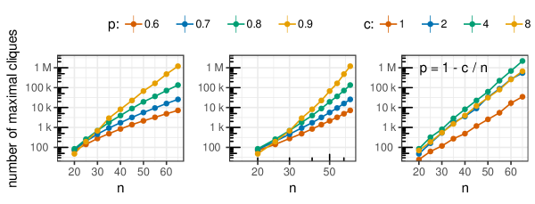
Figure 6: The number of maximal cliques in dense and super-dense $G(n,p)$s. For the left and middle plot, $p$ is constant. For the right plot, $p=1-c/n$ for constant $c$. Note that the $y$-axes are logarithmic and the $x$-axis in the middle plot is logarithmic. Each point is the average of $20$ sampled graphs.

Note that for constant $p$, the left plot with logarithmic $y$-axis is curved downward, indicating sub-exponential scaling, while the middle plot with logarithmic $x$- and $y$-axis is bent upwards, indicating super-polynomial scaling. This is in line with our lower bound in Theorem 2.1.

For the super-dense case, the right plot indicates exponential scaling, in line with Theorem 2.3.

6 Conclusion and Discussion

In this paper, we have investigated the number of maximal cliques in three random graph models: the Erdős–Rényi random graph, the inhomogeneous random graph and the geometric inhomogeneous random graph. We have shown that sparse Erdős–Rényi random graphs only contain a polynomial amount of maximal cliques, but in the other two sparse models, the number of maximal cliques scales at least super-polynomially in the network size. This is caused by the degree-heterogeneity in these models, as many large maximal cliques are present close to the core of these random graphs. We prove that there only exist a linear amount of small maximal cliques. Interestingly, these small maximal cliques are almost always formed by two low-degree vertices, whereas all other vertices are hubs of high degree.

We have then shown that this dominant super-polynomial behavior of the number of maximal cliques often only kicks for extreme network sizes, and that experimentally, lower-order linear terms instead drive the scaling of the number of maximal cliques until large values of the network size. This explains the dichotomy between the theoretical super-polynomial lower bounds for these models, and the observation that in real-world networks, the amount of maximal cliques is often quite small.

Several of our results only constitute lower bounds for the number of maximal cliques. We believe that relatively close upper bounds can be constructed in a similar fashion, but leave this open for further research.

While Theorem 3.7 only holds for 2-norms, we believe that the theorem can be extended to any $L^{p}$-norm for $p\neq 1,\infty$, by looking at the $L^{p}$ norm-cycle instead of the regular cycle. For $p=1,\infty$ this approach fails, shortest distance paths to non-opposing segments pass through the center of the cycle. Therefore, opposing segments are just as close as many non-opposing ones. Whether Theorem 3.7 also holds with 1 or $\infty$ norms is therefore a question for further research. We also believe that this approach also extends to the underlying space $[0,1]^{d}$ for general $d$, where instead of looking at a cycle inside $[0,1]^{2}$, one studies a $d$-ball inscribed in $[0,1]^{d}$ instead.

Appendix A Proof of Theorem 3.10

Lemma A.1.

Let $(A_{i})_{i\in[k]}$ be a set of areas of size $A$, and let $S$ be a set of vertices, such that $A|S|>n^{\varepsilon}$ for some $\varepsilon>0$. Then, for any $0<\lambda<1$ and $k<\exp(\lambda A|S|)$, with high probability all areas contain at least $(1-\lambda)A|S|$ vertices.

Proof.

The Chernoff bound gives for the number of vertices from $S$ within area $A$, $N_{S,A}$:

$$\mathbb{P}\left(N_{S,A}<(1-\lambda)A|S|\right)\leq\exp\Big{(}-\lambda A|S|\Big{)}.$$ (49)

This implies that when $A|S|>n^{\varepsilon}$ for some $\varepsilon>0$, then, with high probability, all areas contain at least $(1-\lambda)A|S|$ vertices. ∎

We follow the same construction of areas and sets as in the proof of Theorem 3.7. By (20) this creates $2k=s\cdot n^{\min(\beta/2,\gamma/2)}$ areas of size $A=n^{-3/2\gamma}$, with on average $\mathbb{E}\left[|S|\right]=n^{(3-\tau)/2-\beta}$ vertices. Thus, Lemma A.1 shows that as long as $\beta+3/2\gamma<(3-\tau)/2$, then all areas contain with high probability at least

$$n^{\prime}=c_{1}n^{(3-\tau)/2-\beta-3/2\gamma}$$

vertices for some $c_{1}>0$.

From (5), it follows that any set of vertices that contains one in each given area still satisfies the requirement that all vertices in non-opposite boxes connect, as in non-opposite boxes, the connection probability equals 1 by (14). Now to form a clique minus a matching, vertices in opposite boxes should not connect.

With high probability, a positive proportion of vertices in two opposing areas have distance at least $t+h=a+n^{-\gamma}$, by the uniform distribution within areas, and the fact that a positive proportion of the two areas have distance $t+h$.

By (5), the probability that vertices $i,j\in S$ at distance at least $a+n^{-\gamma}$ are connected is bounded by

$$p_{ij} \leq\min\Bigg{(}\Big{(}\frac{a^{2}(1-n^{-\beta})}{(a+n^{-\gamma})^{2}}\Big{)}^{1/T},1\Bigg{)}$$

$$=(1-n^{-\beta})(1-n^{-\gamma})(1+o(1))$$

$$=(1-\max(n^{-\beta},n^{-\gamma}))(1+o(1)).$$ (50)

Similarly as in (23),

$$\mathbb{P}\left(M=0\right)\leq k(1-\max(n^{-\beta},n^{-\gamma})^{(n^{\prime})^{2}}\leq k\exp(-\max(n^{-\beta},n^{-\gamma})(n^{\prime})^{2})$$ (51)

Using that $n^{\prime}=c_{1}n^{(3-\tau)/2-\beta-3/2\gamma}$ therefore yields

$$\mathbb{P}\left(M=0\right)\leq k\exp(-c_{1}^{2}n^{(3-\tau)-\beta-3\gamma}\max(n^{-\beta},n^{-\gamma})).$$ (52)

Thus, choosing $\beta=\gamma=(3-\tau)/5-\varepsilon$ ensures that there is a co-matching of size $k=s\cdot n^{(3-\tau)/10-\varepsilon}$ ∎

Appendix B Proof of Lemma 4.3

Proof.

This integral equals

$$\int_{0}^{1}\dots\int_{0}^{1}\int_{0}^{1}\int_{0}^{x_{2}}x_{1}^{k-1-\tau}x_{2}^{k-1-\tau}x_{3}^{2-\tau}\cdots x_{k}^{2-\tau}\exp\Big{(}-\mu^{1-\tau}x_{1}x_{2}^{\tau-2}\Big{)}dx_{1}dx_{2}\dots dx_{k}$$

$$+\int_{0}^{1}\dots\int_{0}^{1}\int_{1}^{\infty}\int_{0}^{x_{2}}x_{1}^{k-1-\tau}x_{2}^{1-\tau}x_{3}^{1-\tau}\cdots x_{k}^{1-\tau}\prod_{i=3}^{k}\min\Big{(}x_{2}x_{i},1\Big{)}\exp\Big{(}-\mu^{1-\tau}x_{1}x_{2}^{\tau-2}\Big{)}dx_{1}dx_{2}\dots dx_{k}$$ (53)

Now

$$\int_{0}^{1}\dots\int_{0}^{1}\int_{0}^{1}\int_{0}^{x_{2}}x_{1}^{k-1-\tau}x_{2}^{k-1-\tau}x_{3}^{2-\tau}\cdots x_{k}^{2-\tau}dx_{2}dx_{1}\dots dx_{k}<\infty,$$ (54)

as $2-\tau>-1$, and $k-1-\tau>-1$ for $k\geq 3$ as well. We now turn to the second integral. The second integral is finite if

$$\int_{0}^{1}\dots\int_{0}^{1}\int_{1}^{\infty}\int_{0}^{x_{2}}x_{1}^{k-1-\tau}x_{2}^{1-\tau}x_{3}^{1-\tau}\cdots x_{k}^{1-\tau}\prod_{i=3}^{k}\min\Big{(}x_{2}x_{i},1\Big{)}\mathbbm{1}_{\left\{x_{2}^{\tau-2}x_{1}<1\right\}}dx_{1}dx_{2}\dots dx_{k}<\infty.$$ (55)

This results in

$$\int_{0}^{1}\dots\int_{0}^{1}\int_{1}^{\infty}\int_{0}^{x_{2}^{2-\tau}}x_{1}^{k-1-\tau}x_{2}^{1-\tau}x_{3}^{1-\tau}\cdots x_{k}^{1-\tau}\prod_{i=3}^{k}\min\Big{(}x_{2}x_{i},1\Big{)}dx_{1}\dots dx_{k}$$

$$=\int_{0}^{1}\dots\int_{0}^{1}\int_{1}^{\infty}x_{2}^{(2-\tau)(k+1-\tau)-1}x_{3}^{1-\tau}\cdots x_{k}^{1-\tau}\prod_{i=3}^{k}\min\Big{(}x_{2}x_{i},1\Big{)}dx_{2}\dots dx_{k}$$ (56)

W.l.o.g. we assume that $x_{3}>x_{4}>\dots>x_{k}$. Then, the inner integral evaluates to

$$\int_{1}^{\infty}x_{2}^{(2-\tau)(k+1-\tau)-1}\prod_{i=3}^{k}\min\Big{(}x_{2}x_{i},1\Big{)}dx_{2}$$

$$=\int_{1}^{1/x_{3}}x_{2}^{(2-\tau)(k+1-\tau)+k-3}x_{3}\cdots x_{k}dx_{2}+\dots+\int_{1/x_{k}}^{\infty}x_{2}^{(2-\tau)(k+1-\tau)-1}dx_{2}$$

$$=C_{3}x_{3}^{(\tau-2)(k+1-\tau)+3-k}x_{4}\cdots x_{k}+C_{4}x_{4}^{(\tau-2)(k+1-\tau)+4-k}x_{5}\cdots x_{k}+\dots+C_{k}x_{k}^{(\tau-2)(k+1-\tau)}$$ (57)

We now show that all these terms evaluate to a finite integral when plugged into (B). Indeed,

$$\int_{0}^{1}\int_{0}^{x_{3}}\dots\int_{0}^{x_{k-1}}x_{l}^{(\tau-2)(k+1-\tau)+l-k}x_{l+1}\cdots x_{k}x_{3}^{1-\tau}\cdots x_{k}^{1-\tau}dx_{k}dx_{k-1}\dots dx_{3}$$

$$=\int_{0}^{1}\int_{0}^{x_{3}}\dots\int_{0}^{x_{l-1}}x_{l}^{(\tau-2)(l-\tau)-1}x_{3}^{1-\tau}\cdots x_{l-1}^{1-\tau}dx_{l}dx_{l-1}\dots dx_{3}$$

$$=\int_{0}^{1}\int_{0}^{x_{3}}\dots\int_{0}^{x_{l-2}}x_{l-1}^{(\tau-2)(l-1-\tau)-1}x_{3}^{1-\tau}\cdots x_{l-2}^{1-\tau}dx_{l}dx_{l-2}\dots dx_{3}<\infty$$ (58)

as the index $l-k$ remains at least 3. Therefore, (32) is finite as well. ∎

References

- [1] T. Bläsius, C. Freiberger, T. Friedrich, M. Katzmann, F. Montenegro-Retana, and M. Thieffry. Efficient shortest paths in scale-free networks with underlying hyperbolic geometry. ACM Trans. Algorithms, 18(2), 2022.
- [2] T. Bläsius, T. Friedrich, and A. Krohmer. Cliques in hyperbolic random graphs. Algorithmica, 80(8):2324–2344, 2018.
- [3] T. Bläsius and P. Fischbeck. On the external validity of average-case analyses of graph algorithms. In European Symposium on Algorithms (ESA), pages 21:1–21:14, 2022.
- [4] T. Bläsius, T. Friedrich, M. Katzmann, U. Meyer, M. Penschuck, and C. Weyand. Efficiently generating geometric inhomogeneous and hyperbolic random graphs. Network Science, 10(4):361–380, 2022.
- [5] T. Bläsius, T. Friedrich, and A. Krohmer. Hyperbolic random graphs: Separators and treewidth. In European Symposium on Algorithms (ESA), pages 15:1–15:16, 2016.
- [6] M. Boguñá, F. Papadopoulos, and D. Krioukov. Sustaining the internet with hyperbolic mapping. Nat. Commun., 1(6):1–8, 2010.
- [7] K. Bringmann, R. Keusch, and J. Lengler. Geometric inhomogeneous random graphs. Theoretical Computer Science, 760:35–54, feb 2019.
- [8] D. Eppstein, M. Löffler, and D. Strash. Listing all maximal cliques in sparse graphs in near-optimal time. In International Symposium on Algorithms and Computation (ISAAC), pages 403–414, 2010.
- [9] D. Eppstein, M. Löffler, and D. Strash. Listing all maximal cliques in large sparse real-world graphs. ACM Journal of Experimental Algorithmics (JEA), 18, 2013.
- [10] D. Eppstein and D. Strash. Listing all maximal cliques in large sparse real-world graphs. In Symposium on Experimental and Efficient Algorithms (SEA), pages 364–375, 2011.
- [11] G. García-Pérez, M. Boguñá, A. Allard, and M. Á. Serrano. The hidden hyperbolic geometry of international trade: World trade atlas 1870–2013. Sci. Rep., 6(1), 2016.
- [12] R. van der Hofstad. Random Graphs and Complex Networks Vol. 1. Cambridge University Press, 2017.
- [13] R. van der Hofstad, J. S. H. van Leeuwaarden, and C. Stegehuis. Optimal subgraph structures in scale-free configuration models. The Annals of Applied Probability, 31(2), 2021.
- [14] M. Kiwi and D. Mitsche. Spectral gap of random hyperbolic graphs and related parameters. The Annals of Applied Probability, 28(2):941–989, apr 2018.
- [15] R. Kleinberg. Geographic routing using hyperbolic space. In IEEE INFOCOM 2007 - 26th IEEE International Conference on Computer Communications. IEEE, 2007.
- [16] D. Krioukov, F. Papadopoulos, M. Kitsak, A. Vahdat, and M. Boguná. Hyperbolic geometry of complex networks. Phys. Rev. E, 82(3):036106, 2010.
- [17] J. Lengler and L. Todorovic. Existence of small separators depends on geometry for geometric inhomogeneous random graphs.
- [18] R. Michielan and C. Stegehuis. Cliques in geometric inhomogeneous random graphs. 10(1).
- [19] S. Tsukiyama, M. Ide, H. Ariyoshi, and I. Shirakawa. A new algorithm for generating all the maximal independent sets. SIAM Journal on Computing, 6(3):505–517, sep 1977.
- [20] H. Yamaji. On the number of maximal cliques in two-dimensional random geometric graphs: Euclidean and hyperbolic. Mar. 2023.