Multivariate Matérn Models – A Spectral Approach

Abstract

The classical Matérn model has been a staple in spatial statistics. Novel data-rich applications in environmental and physical sciences, however, call for new, flexible vector-valued spatial and space-time models. Therefore, the extension of the classical Matérn model has been a problem of active theoretical and methodological interest. In this paper, we offer a new perspective to extending the Matérn covariance model to the vector-valued setting. We adopt a spectral, stochastic integral approach, which allows us to address challenging issues on the validity of the covariance structure and at the same time to obtain new, flexible, and interpretable models. In particular, our multivariate extensions of the Matérn model allow for time-irreversible or, more generally, asymmetric covariance structures. Moreover, the spectral approach provides an essentially complete flexibility in modeling the local structure of the process. We establish closed-form representations of the cross-covariances when available, compare them with existing models, simulate Gaussian instances of these new processes, and demonstrate estimation of the model’s parameters through maximum likelihood. An application of the new class of multivariate Matérn models to environmental data indicate their success in capturing inherent covariance-asymmetry phenomena.

, , and

t1Partially supported by NSF Grant DGE-1841052 t2Supported by NSF Grant DMS-1916226

1 Introduction and main ideas

In the past two decades, there have been considerable interests in modeling vector-valued spatial processes, especially in the context of environmental data (cf. Genton and Kleiber,, 2015). One popular model for such processes is the multivariate Matérn model, which extends the Matérn model to the multivariate case and was first introduced in Gneiting et al., (2010). Extensions, improvements, and analysis of multivariate Matérn models are numerous (for more information and examples, see Porcu et al.,, 2023; Alegría et al.,, 2021; Apanasovich et al.,, 2012; Emery et al.,, 2022; Genton and Kleiber,, 2015; Kleiber,, 2018). Section 3 of Genton and Kleiber, (2015) and Section 5.2 of Porcu et al., (2023) review multivariate Matérn models.

Let $\boldsymbol{Y}(\boldsymbol{s})=(Y_{i}(\boldsymbol{s}))_{i=1}^{p}$ denote a zero-mean stochastic process with finite variance taking values in $\mathbb{R}^{p},\ p\geq 1$, and indexed by $\boldsymbol{s}\in\mathbb{R}^{d}$. Unless stated otherwise, all vectors we consider will be column-vectors, and they will be denoted with boldface letters to distinguish them from scalars.

Most of the existing multivariate extensions of the Matérn model start by prescribing a Matérn-like cross-covariance function for $\boldsymbol{Y}=\{\boldsymbol{Y}(\boldsymbol{s}),\ \boldsymbol{s}\in\mathbb{R}^{d}\}$, or some modification of one. While natural and appealing, this leads to formidable challenges in verifying the validity (positive definiteness) of the resulting matrix-valued auto-covariance. One consequence of this approach is that many of the existing multivariate Matérn models are covariance reversible, i.e., $\mathbb{E}[\boldsymbol{Y}(\boldsymbol{s})\boldsymbol{Y}(\boldsymbol{t})^{\top}]=\mathbb{E}[\boldsymbol{Y}(\boldsymbol{t})\boldsymbol{Y}(\boldsymbol{s})^{\top}]$, for all $\boldsymbol{s},\,\boldsymbol{t}\in\mathbb{R}^{d}$. While this property is clearly automatic in the case when $\boldsymbol{Y}(\boldsymbol{t})$ is scalar-valued ($p=1$), it is an exception rather than the norm in the vector-valued case ($p\geq 2$). This observation shows that the existing covariance-reversible multivariate Matérn models are rather restrictive. Lastly, while the classical Matérn is well understood, the local behavior of the multivariate Matérn-type models is largely unexplored. We will give a more comprehensive overview of the existing literature on multivariate Matérn models in Section 2.2.

In this paper, we aim to address the above challenges by adopting a stochastic integral perspective to the construction of the multivariate Matérn models. This will allow us to automatically obtain valid covariance structures with interpretable parameterizations and obtain a rich family of vector-valued models including reversible as well as non-reversible covariance structures.

Recall that $\boldsymbol{Y}$ is said to be second-order stationary if its covariance function

$$\boldsymbol{C}_{\boldsymbol{Y}}(\boldsymbol{h}):=\mathbb{E}[\boldsymbol{Y}(\boldsymbol{h})\boldsymbol{Y}(\boldsymbol{0})^{\top}]$$

is defined and depends only on the lag $\boldsymbol{h}\in\mathbb{R}^{d}$. Note that for $p\geq 2$, the function $\boldsymbol{h}\mapsto\boldsymbol{C}_{\boldsymbol{Y}}(\boldsymbol{h})$ is $p\times p$-matrix valued, and as in the classical scalar-valued setting ($p=1$), is positive (semi)definite in the sense that

$$\sum_{i,j=1}^{n}a_{i}a_{j}\boldsymbol{C}_{\boldsymbol{Y}}(\boldsymbol{s}_{i}-\boldsymbol{s}_{j})$$ (1.1)

is a positive semi-definite matrix for all $a_{i}\in\mathbb{R}$ and points $\boldsymbol{s}_{i}\in\mathbb{R}^{d}$, $i=1,\dots,n$. A more detailed review of the spectral theory for vector-valued second-order stationary processes is given in Section 2.1, below.

To illustrate ideas, consider for a moment the scalar-valued case $p=1$. If $Y=\{Y(\boldsymbol{s}),\ \boldsymbol{s}\in\mathbb{R}^{d}\}$ is zero-mean, second-order stationary and $L^{2}-$continuous, a classical result due to Cramér, (1942) yields the following spectral representation of $Y$ as a stochastic integral:

$$Y(\boldsymbol{s})=\int_{\mathbb{R}^{d}}e^{\mathbbm{i}\langle\boldsymbol{s},\boldsymbol{x}\rangle}\xi(d\boldsymbol{x}),$$ (1.2)

which is valid almost surely for each $\boldsymbol{s}\in\mathbb{R}^{d}$, where the integration is with respect to a random, complex-valued measure $\xi$ with mean zero and orthogonal increments. Namely, we have that $\mathbb{E}[\xi(A)]=0$, $\xi(A\cup B)=\xi(A)+\xi(B)$, for $A\cap B=\emptyset$, and for a finite Borel measure $F_{Y}$ on $\mathbb{R}^{d}$, we have $\mathbb{E}[\xi(A)\overline{\xi(B)}]=F_{Y}(A\cap B),$ for all Borel sets $A,B\subset\mathbb{R}^{d}$ (cf. Section 2.1 below). Relation (1.2) readily implies that the auto-covariance of $Y$ is

$$C_{Y}(\boldsymbol{h})=\mathbb{E}[Y(\boldsymbol{t}+\boldsymbol{h})Y(\boldsymbol{t})]=\int_{\mathbb{R}^{d}}e^{\mathbbm{i}\langle\boldsymbol{h},\boldsymbol{x}\rangle}F_{Y}(d\boldsymbol{x})$$ (1.3)

for $\boldsymbol{h},\boldsymbol{t}\in\mathbb{R}^{d}$, so that $F_{Y}(d\boldsymbol{x})=\mathbb{E}[|\xi(d\boldsymbol{x})|^{2}]$ is precisely the spectral measure of the process $Y,$ per the classical Bochner Theorem (see Theorem 2.2).

Since the process $Y$ in (1.2) is real-valued, the random measure $\xi$ is necessarily Hermitian, i.e., $\xi(-A)=\overline{\xi(A)}$, and the spectral measure $F_{Y}$ is real and symmetric, i.e., $\overline{F_{Y}(-A)}=F_{Y}(A)$ (Proposition 2.6). If $F_{Y}$ has a density $f_{Y}$ with respect to the Lebesgue measure, then $f_{Y}$ is referred to as the spectral density of the process $Y.$

We illustrate these fundamental notions with the classical Matérn covariance in $\mathbb{R}^{d},\ d\geq 1$. Recall that a scalar-valued second-order stationary process $Y=\{Y(\boldsymbol{s}),\ \boldsymbol{s}\in\mathbb{R}^{d}\}$ is said to follow the Matérn model if its auto-covariance and spectral measures are respectively:

$$\begin{split}C_{Y}(\boldsymbol{h})&={\cal M}(\|\boldsymbol{h}\|;a,\nu,\sigma^{2})\\ &:=\frac{\sigma^{2}2^{1-\nu}}{\Gamma(\nu)}(a\|\boldsymbol{h}\|)^{\nu}\mathcal{K}_{\nu}(a\|\boldsymbol{h}\|),\end{split}$$ (1.4)

$$f_{d,(a,\nu,\sigma^{2})}(\boldsymbol{x})d\boldsymbol{x} =\frac{\sigma^{2}c(d,\nu,a)^{2}}{\left(a^{2}+\|\boldsymbol{x}\|^{2}\right)^{\nu+\frac{d}{2}}}d\boldsymbol{x},$$ (1.5)

where $\|\cdot\|$ denotes the Euclidean norm in $\mathbb{R}^{d}$, $c(d,\nu,a)^{2}=a^{2\nu}\Gamma(\nu+d/2)/(\pi^{d/2}\Gamma(\nu))$, $\Gamma(\cdot)$ is the Euler gamma function, and $\mathcal{K}_{\nu}(\cdot)$ is the modified Bessel function of the second kind with order $\nu$ (page 48, Stein,, 1999). The parameterization is such that $\sigma^{2}=C_{Y}(\boldsymbol{0})={\rm Var}(Y(\boldsymbol{t}))$ is the marginal variance of the model, $a>0$ is the inverse range, and $\nu>0$ is the shape or smoothness parameter. Observe that $C_{Y}(\boldsymbol{h})$ is isotropic and valid, i.e., positive semi-definite for every $d\geq 1$. The latter property is closely related to an important result due to Schoenberg, (1938), which we discuss in Section F where we also give a simple derivation of (1.5) from (1.4).

In the rest of this section, we sketch the main ideas behind our approach for $d=1$. A more systematic exposition for all $d$ is given in Section 4. We begin with the scalar-valued case of $p=1$.

Consider a complex Gaussian measure $B(dx)$ on $\mathbb{R}$ with orthogonal increments such that $B(dx)=\overline{B(-dx)}$ and $\mathbb{E}[|B(dx)|^{2}]=\sigma^{2}\cdot dx$, where $dx$ stands for Lebesgue measure and $\sigma>0$. Letting

$$\xi(dx):=c(1,\nu,a)\left(a^{2}+x^{2}\right)^{\left(-\nu-\frac{1}{2}\right)/2}B(dx),$$ (1.6)

in view of (1.5), we obtain $\mathbb{E}\left[|\xi(dx)|^{2}\right]=f_{1,(a,\nu,\sigma^{2})}(x)dx$. Hence by (1.3) the stochastic integral in (1.2) defines a stationary Gaussian process with the Matérn auto-covariance ${\cal M}(\cdot;a,\nu,\sigma^{2})$. Alternatively, since

$$\left|(a\pm\mathbbm{i}x)^{-\nu-\frac{1}{2}}\right|^{2}=\left(a^{2}+x^{2}\right)^{-\nu-\frac{1}{2}},$$

where $\pm$ is either $+$ or $-$, one could take

$$\xi(dx)=c(1,\nu,a)\left(a\pm\mathbbm{i}x\right)^{-\nu-\frac{1}{2}}B(dx).$$ (1.7)

This choice also yields $\mathbb{E}[|\xi(dx)|^{2}]=f_{1,(a,\nu,\sigma^{2})}(x)dx$ and hence the stochastic integral (1.2) defines a processes with the same Matérn covariance for $d=1$. We will primarily focus on this second representation in (1.7), since it will naturally lead to general complex-valued spectral densities and potentially non-reversible models for $p\geq 2$ (in Sections 3 and 4). The restriction $a>0$ ensures that powers of the complex number $a\pm\mathbbm{i}x$ are well-defined by avoiding the singularity at the origin of the complex plane.

We now turn to multivariate Matérn, that is, where $p>1$. Motivated by the Cramér stochastic integral representation (1.2) of the classical Matérn process with (1.7), we consider

$$\boldsymbol{Y}(s)=\int_{\mathbb{R}}e^{\mathbbm{i}sx}\boldsymbol{\xi}(dx),\mbox{and }\boldsymbol{\xi}(dx):=\boldsymbol{P}(x)\boldsymbol{B}(dx).$$ (1.8)

Now, however, the term $(a+\mathbbm{i}x)^{-\nu-1/2}$ in (1.7) is replaced by a $\mathbb{C}^{p\times p}$-valued function $\boldsymbol{P}(x)$, while $\boldsymbol{B}(dx)$ is a $\mathbb{C}^{p}$-vector-valued counterpart to the random measure $B(dx)$. Specifically, we consider

$$\boldsymbol{P}(x):=\textrm{diag}(c_{j}\cdot(a_{j}+\mathbbm{i}x)^{-\nu_{j}-\frac{1}{2}},j=1,\dots,p)\in\mathbb{C}^{p\times p},$$

with normalizing constants $c_{j}:=c(1,\nu_{j},a_{j})$ and parameters $a_{j}>0$ and $\nu_{j}>0,\ j=1,\cdots,p$.

On the other hand, the vector-valued zero-mean random measure $\boldsymbol{B}(dx)\in\mathbb{C}^{p}$ in (1.8) is assumed to be Hermitian $\boldsymbol{B}(dx)=\overline{\boldsymbol{B}(-dx)}$, to have orthogonal increments (cf. Definition 2.4), where

$$\boldsymbol{\mu}(dx): =\mathbb{E}\left[\boldsymbol{B}(dx)\overline{\boldsymbol{B}(dx)}^{\top}\right]$$

$$=\left(\Re(\boldsymbol{\Sigma}_{H})+\textrm{sign}(x)\mathbbm{i}\Im(\boldsymbol{\Sigma}_{H})\right)dx$$

for some self-adjoint and positive-semidefinite matrix $\boldsymbol{\Sigma}_{H}=(\sigma_{jk})_{p\times p}$. That is, $\boldsymbol{\Sigma}_{H}=\boldsymbol{\Sigma}_{H}^{*}:=\overline{\boldsymbol{\Sigma}_{H}}^{\top}$, and the quadratic forms $\boldsymbol{x}^{\top}\boldsymbol{\Sigma}_{H}\boldsymbol{x}\geq 0$, for all $\boldsymbol{x}\in\mathbb{C}^{p}$. Here, $\Re(\cdot)$ and $\Im(\cdot)$ denote the real and imaginary part functions, and $\textrm{sign}(x)=\mathbb{I}(x>0)-\mathbb{I}(x<0)$ where $\mathbb{I}(\cdot)$ is the indicator function.

By (1.8), one can show that

$$\boldsymbol{C}_{\boldsymbol{Y}}(h) =\mathbb{E}[\boldsymbol{Y}(t+h)\boldsymbol{Y}(t)^{\top}]$$

$$=\int_{\mathbb{R}}e^{\mathbbm{i}hx}\boldsymbol{P}(x)\boldsymbol{\mu}(dx)\overline{\boldsymbol{P}(x)}$$

$$=\int_{\mathbb{R}}e^{\mathbbm{i}hx}\boldsymbol{F}(dx),$$

where $\boldsymbol{F}(dx)=(F_{jk}(dx))_{p\times p}:=\boldsymbol{P}(x)\boldsymbol{\mu}(dx)\overline{\boldsymbol{P}(x)}$ is now the matrix-valued spectral measure of $\boldsymbol{Y}$. (The definition and integration with respect to the measure $\boldsymbol{F}(dx)$ is discussed in Section 2.1.)

The spectral measure $\boldsymbol{F}$ takes values in the space of all self-adjoint and positive-semidefinite ${p\times p}$ matrices. In contrast with the scalar case ($p=1$), however, the spectral measure $\boldsymbol{F}$ may have complex components. In fact, $\boldsymbol{F}$ is real if and only if the process $\boldsymbol{Y}$ is covariance reversible (Proposition 2.9).

To gain some intuition and to connect to some of the existing multivariate Matérn models, let $1\leq j,k\leq p$, and consider the cross-covariances:

$$C_{jk}(h) =[\boldsymbol{C}_{\boldsymbol{Y}}(h)]_{jk}={\rm Cov}(Y_{j}(t+h),Y_{k}(t))$$

$$\begin{split}&=c_{j}c_{k}\int_{\mathbb{R}}e^{\mathbbm{i}hx}(a_{j}+\mathbbm{i}x)^{-\nu_{j}-\frac{1}{2}}\\ &~{}~{}~{}~{}~{}~{}~{}~{}~{}~{}~{}~{}~{}~{}~{}\times(\Re(\sigma_{jk})+\textrm{sign}(x)\mathbbm{i}\Im(\sigma_{jk}))\\ &~{}~{}~{}~{}~{}~{}~{}~{}~{}~{}~{}~{}~{}~{}~{}\times(a_{k}-\mathbbm{i}x)^{-\nu_{k}-\frac{1}{2}}dx.\end{split}$$ (1.9)

This shows that the univariate components of $\boldsymbol{Y}(s)=(Y_{j}(s))_{j=1}^{p},\ s\in\mathbb{R}$, have Matérn auto-covariances. Indeed, since $\boldsymbol{\Sigma}_{H}=\overline{\boldsymbol{\Sigma}_{H}}^{\top}$, we have $\Im(\sigma_{jj})=0$, and in fact $\Re(\sigma_{jj})=\sigma_{jj}\geq 0$ by the positivity of $\boldsymbol{\Sigma}_{H}$. Thus, in view of (1.9), the process $\{Y_{j}(s),\ s\in\mathbb{R}\}$ has precisely the Matérn spectral density in (1.5) with parameters $a_{j}$, $\nu_{j}$, and $\sigma_{jj}$, provided $c_{j}:=c(1,\nu_{j},a_{j})$. (Note that the diagonal terms $\sigma_{jj}$ now refer to marginal variance parameters.)

Having non-zero off-diagonal entries in $\boldsymbol{\Sigma}_{H}$ is a simple and yet flexible way to model the cross-covariance structure between the components of $\boldsymbol{Y}$. We give next some intuition. In the special case when $\sigma_{jk}$ is real and $\nu_{j}=\nu_{k}=\nu$, $a_{j}=a_{k}=a$, and $c_{j}=c_{k}=c(1,\nu,a)$, for example, we obtain

$${\rm Cov}(Y_{j}(t),Y_{k}(s)) =\sigma_{jk}\cdot c(1,\nu,a)^{2}$$

$$~{}~{}~{}~{}~{}~{}\times\int_{\mathbb{R}}e^{\mathbbm{i}(t-s)x}(a^{2}+x^{2})^{-\nu-\frac{1}{2}}dx$$

$$=\sigma_{jk}{\cal M}(|t-s|;a,\nu,1),$$

so that $\sigma_{jk}$ may be interpreted as the (lag-independent) cross-covariance between the one-dimensional Matérn processes $Y_{j}$ and $Y_{k}$. In this case, the bi-variate process $\{(Y_{j}(t),Y_{k}(t))^{\top},\ t\in\mathbb{R}\}$ has a real spectral measure, and it is covariance-reversible, i.e., ${\rm Cov}(Y_{j}(t),Y_{k}(s))={\rm Cov}(Y_{j}(s),Y_{k}(t))$. Even if $\sigma_{jk}$ is real, however, when $\nu_{j}\not=\nu_{k}$ or $a_{j}\neq a_{k}$, we obtain that ${\rm Cov}(Y_{j}(t),Y_{k}(s))\not\equiv{\rm Cov}(Y_{j}(s),Y_{k}(t))$, for all $s,t\in\mathbb{R}$. The closed-form expression of the resulting non-reversible cross-covariances is established in Theorem 3.1 below in terms of a Whittaker special function. The possibility to have complex $\sigma_{jk}$’s adds even more flexibility to the model and the closed-form expression of the cross-covariances in the purely imaginary case ($\Re(\sigma_{jk})=0$), is established in Theorem 3.11 below. It involves the modified Struve and modified Bessel functions of the first kind. By combining the cases of real and imaginary $\sigma_{jk}$’s one obtains the general closed-form of the cross-covariances of this novel class of models (cf. Section 3.3, below).

For general $d$, our construction results in anisotropic cross-covariances that are non-reversible. In much of spatial statistics, there is a focus on geometric anisotropy, where $C_{jk}(\boldsymbol{h})=C_{iso}(\sqrt{\boldsymbol{h}^{\top}Q\boldsymbol{h}})$ for a positive definite matrix $Q$ and isotropic covariance function $C_{iso}(\cdot)$ (Chiles and Delfiner,, 2012). There is also an interest in zonal isotropy, where the covariance only depends on some elements of $\boldsymbol{h}$ (Chiles and Delfiner,, 2012). Here, we introduce cross-covariances that have more general and complex anisotropic structure.

Our work uses the form of (1.7) to construct multivariate Matérn models, while Bolin and Wallin, (2019) used instead (1.6), where they also essentially take $\boldsymbol{\mu}(dx)=\Re(\boldsymbol{\Sigma}_{H})dx$ in our notation. This results only in symmetric (reversible) models with $\boldsymbol{C}(h)=\boldsymbol{C}(-h)$ for all $h\in\mathbb{R}$ (see also Section 6.3, below, for more details). We advocate for using (1.7) because, as illustrated, one obtains a more flexible family of models, which in many cases continue to enjoy closed-form expressions for their cross-covariances.

The remainder of the paper is structured as follows. In Section 2, we review spectral theory and the notion of covariance-reversibility of multivariate processes. This section is technical, and some details may be omitted by the reader. We also review the literature on multivariate Matérn models in more detail. In Section 3, we comprehensively address the case of $d=1$ as presented here in the introduction. First, in Section 3.1 we find all closed-form expressions and explore the class of models that have real directional measure with $\Im(\sigma_{jk})=0$ in (1.9). We next consider a second class of asymmetric models with imaginary or complex directional measure, i.e., $\Im(\sigma_{jk})\neq 0$, in Section 3.2.

We then introduce a model for general $d\in\{1,2,3,\dots\}$ in Section 4. Although closed-form representations of the cross-covariances are not often available for $d>1$, one can readily numerically approximate them using fast Fourier transforms. Furthermore, simulating processes based on these multivariate spatial cross-covariances is straightforward due to Emery et al., (2016).

In Section 5, we estimate the proposed model based on two datasets previously studied in the multivariate Matérn literature: the pressure and temperature data in the North American Pacific Northwest (studied in, among many others, Gneiting et al.,, 2010) and the Argo temperature data of the ocean at two different depths (Argo,, 2020), studied in Bolin and Wallin, (2019). The proposed model can have comparable and at times improved model fit in terms of the Akaike information criterion (AIC) compared to Gneiting et al., (2010). The estimated model shows evidence of a complex-valued directional measure, hence irreversibility, in the cross-covariance for the Argo temperature data. We then outline a number of areas for future research in Section 6.

All code used to present results in the paper is available at https://github.com/dyarger/multivariate_matern, where we also provide an R Shiny application that computes and plots the cross-covariances introduced here. The Appendix contains further results on these multivariate Matérn models. Most notably, in Section E, we describe the tangent processes of the introduced multivariate Matérn models. The tangent processes describe the (scaled) local behavior of the multivariate Matérn processes, and, in the Gaussian case, they are operator fractional Brownian fields (OFBFs), an extension of fractional Brownian fields to the vector-valued setting (Didier et al.,, 2018; Didier and Pipiras,, 2011). See Shen et al., (2022) and references therein for more background on tangent processes. We establish that our family of Matérn-type models can realize essentially all possible OFBF tangent fields, thus providing maximal flexibility in the local behavior of the multivariate processes.

2 Spectral theory and multivariate Matérn models – an overview

In this section, for the sake of completeness, we first review some fundamental results on the spectral representation of vector-valued processes. We then discuss our contributions in the context of the recent and expanding literature on multivariate Matérn and multivariate spatial processes.

2.1 The multivariate Bochner and Cramér theorems

We provide a treatment of the mathematical background behind the spectral properties of multivariate, second-order stationary spatial processes $\boldsymbol{Y}=\{\boldsymbol{Y}(\boldsymbol{s}),\ \boldsymbol{s}\in\mathbb{R}^{d}\}$ taking values in $\mathbb{C}^{p}$ over the field of complex numbers $\mathbb{C}$. The classical theorems of Bochner and Cramér are at the foundation of spectral analysis of second-order processes and random fields. These theorems also have far-reaching extensions to multivariate processes (Hannan,, 1970; Yaglom,, 1987; Gelfand and Banerjee,, 2010) and, more generally, processes taking values in separable Hilbert spaces (see, e.g., Neeb,, 1998; Shen et al.,, 2022, and the references therein). Below, will confine attention to the multivariate case. However, keep in mind that much of what we present has infinite-dimensional extensions.

We will equip $\mathbb{C}^{p}$ with the Euclidean inner product $\langle\boldsymbol{x},\boldsymbol{y}\rangle=\boldsymbol{x}^{\top}\overline{\boldsymbol{y}}=\sum_{j=1}^{p}x_{j}\overline{y}_{j}$ and corresponding norm $\|\boldsymbol{x}\|:=\sqrt{\langle\boldsymbol{x},\boldsymbol{x}\rangle}$. Let $L^{2}(\mathbb{C}^{p})$ denote the class of $\mathbb{C}^{p}$-valued random elements $\boldsymbol{Y}$ defined on a common probability space such that $\mathbb{E}[\|\boldsymbol{Y}\|^{2}]<\infty$. An $\mathbb{C}^{p}$-valued stochastic process $\{\boldsymbol{Y}(\boldsymbol{s}),\ \boldsymbol{s}\in\mathbb{R}^{d}\}$ will be referred to as second-order if $\boldsymbol{Y}(\boldsymbol{s})\in L^{2}(\mathbb{C}^{p})$ for all $\boldsymbol{s}$.

The cross-covariance of two zero-mean random vectors $\boldsymbol{X}$ and $\boldsymbol{Y}$ in $L^{2}(\mathbb{C}^{p})$ is defined as the matrix

$$\boldsymbol{C}(\boldsymbol{X},\boldsymbol{Y}):=\mathbb{E}\left[\boldsymbol{X}\overline{\boldsymbol{Y}}^{\top}\right]=\Big{(}\mathbb{E}\left[X_{j}\overline{Y}_{k}\right]\Big{)}_{p\times p}.$$ (2.1)

Since $\left(\boldsymbol{X}\overline{\boldsymbol{Y}}^{\top}\right)^{*}=\boldsymbol{Y}\overline{\boldsymbol{X}}^{\top},$ we have that $\boldsymbol{C}(\boldsymbol{X},\boldsymbol{Y})^{*}=\boldsymbol{C}(\boldsymbol{Y},\boldsymbol{X})$, where $\boldsymbol{A}^{*}$ denotes the conjugate transpose matrix of $\boldsymbol{A}$. In particular the covariance matrix of $\boldsymbol{Y}$, $\boldsymbol{C}(\boldsymbol{Y},\boldsymbol{Y})$ is positive semidefinite. Recall that a complex matrix $\boldsymbol{A}$ of dimension $p\times p$ is said to be positive semidefinite or just positive if $\langle\boldsymbol{A}\boldsymbol{x},\boldsymbol{x}\rangle\geq 0$ for all $\boldsymbol{x}\in\mathbb{C}^{p}$, which necessarily implies that $\boldsymbol{A}$ is Hermitian, i.e., $\boldsymbol{A}=\boldsymbol{A}^{*}$. For convenience, we shall denote the class of complex $p\times p$ matrices as $\mathbb{T}$ and the subclass of positive matrices as $\mathbb{T}_{+}$.

Definition 2.1.

A zero-mean second-order $\mathbb{C}^{p}$-valued stochastic process $\{\boldsymbol{Y}(\boldsymbol{s}),\ \boldsymbol{s}\in\mathbb{R}^{d}\}$ is said to be covariance stationary if its cross-covariance function $\boldsymbol{C}(\boldsymbol{Y}(\boldsymbol{t}),\boldsymbol{Y}(\boldsymbol{s}))$ depends only on the lag $\boldsymbol{t}-\boldsymbol{s}$, in which case define

$$\boldsymbol{C}(\boldsymbol{h}):=\mathbb{E}\left[\boldsymbol{Y}(\boldsymbol{h})\overline{\boldsymbol{Y}(\boldsymbol{0})}^{\top}\right],\ \ \boldsymbol{h}\in\mathbb{R}^{d},$$ (2.2)

which is said to be the stationary (matrix-valued) covariance function of $\{\boldsymbol{Y}(\boldsymbol{s}),\boldsymbol{s}\in\mathbb{R}^{d}\}$.

As with scalar-valued processes, the stationary matrix-valued covariance functions are positive semi-definite in the sense that:

$$\sum_{j,k=1}^{n}\langle\boldsymbol{C}(\boldsymbol{s}_{j}-\boldsymbol{s}_{k})\boldsymbol{x}_{j},\boldsymbol{x}_{k}\rangle\geq 0,$$ (2.3)

for all $\boldsymbol{s}_{j}\in\mathbb{R}^{d},\ \boldsymbol{x}_{j}\in\mathbb{C}^{p},\ j=1,\dots,n$ and $n\in\mathbb{N}$. This is immediate from the fact that the left-hand-side of (2.3) equals $\mathbb{E}|\sum_{j=1}^{n}\langle\boldsymbol{x}_{j},\boldsymbol{Y}(\boldsymbol{s}_{j})\rangle|^{2}\geq 0$. Interestingly, at least for the class of continuous functions $\boldsymbol{C}(\cdot)$, the above property is equivalent to the seemingly weaker requirement that

$$\sum_{j,k=1}^{n}a_{j}\overline{a}_{k}\boldsymbol{C}(\boldsymbol{s}_{j}-\boldsymbol{s}_{k})\in\mathbb{T}_{+}$$ (2.4)

for all $a_{j}\in\mathbb{C},\ \boldsymbol{s}_{j}\in\mathbb{R}^{d},\ j=1,\dots,n$ (see, e.g., Corollary 4.4 in Shen et al.,, 2020).

The next result extends the celebrated characterization of continuous positive-definite functions due to Bochner (see, e.g., Bochner,, 1948). Various versions of this result have appeared in the literature; see, for example, Kallianpur and Mandrekar, (1971), Holmes, (1979), Neeb, (1998), Durand and Roueff, (2022) and van Delft and Eichler, (2020). For a self-contained proof, see Theorem 4.2 in Shen et al., (2020). In the following, a $\mathbb{T}_{+}$-valued set function $F$ on $\mathcal{B}(\mathbb{R}^{d})$ is said to be a $\mathbb{T}_{+}$-valued measure if it is $\sigma$-additive and $|F_{ij}(\mathbb{R}^{d})|<\infty$ for all $i,j=1,\dots,p$.

Theorem 2.2 (Bochner).

Let $\boldsymbol{C}:\mathbb{R}^{d}\to\mathbb{T}$ be continuous in each of its entries at $\boldsymbol{0}$. The matrix-valued function $\boldsymbol{C}$ is positive semidefinite in the sense of (2.4) if and only if there exists a finite $\mathbb{T}_{+}-$valued measure $\boldsymbol{F}$ on $(\mathbb{R}^{d},{\cal B}(\mathbb{R}^{d}))$ such that

$$\boldsymbol{C}(\boldsymbol{s})=\int_{\mathbb{R}^{d}}e^{\mathbbm{i}\langle\boldsymbol{s},\boldsymbol{x}\rangle}\boldsymbol{F}(d\boldsymbol{x}),\ \ \boldsymbol{s}\in\mathbb{R}^{d}.$$ (2.5)

In this case, the measure $\boldsymbol{F}$ is unique and $\boldsymbol{C}:\mathbb{R}^{d}\to\mathbb{T}$ is uniformly continuous in each of its entries. Conversely, for every finite $\mathbb{T}_{+}-$valued measure $\boldsymbol{F}$, Relation (2.5) defines a positive semidefinite function in the sense of (2.3).

When $\boldsymbol{C}$ is the matrix-valued auto-covariance function of a second-order process $\boldsymbol{Y}$, the measure $\boldsymbol{F}$ in (2.5) is referred to as the spectral measure of $\boldsymbol{Y}$. In contrast to the scalar case, however, the spectral measure is now $\mathbb{C}^{p}$-valued and for each Borel set $A$, $\boldsymbol{F}(A)$ is simply a $p\times p$ positive-semidefinite and self-adjoint matrix, so that in particular

$$F_{jk}(A)=\overline{F_{kj}(A)},\ j,k\in\{1,2,\dots,p\}.$$

In this case, the integration in (2.5) can be viewed component-wise with respect to the signed complex measures $F_{jk}(d\boldsymbol{x})$.

Remark 2.3.

When there exists a measurable function $\boldsymbol{f}:\mathbb{R}^{d}\to\mathbb{T}$, such that $\boldsymbol{F}(A)=\int_{A}\boldsymbol{f}(\boldsymbol{x})d\boldsymbol{x},$ $A\in{\cal B}(\mathbb{R}^{d}),$ then $\boldsymbol{f}$ is referred to as the spectral density of $\boldsymbol{C}$. One sufficient condition for the existence of a spectral density is that all the entries of $\boldsymbol{C}$ are integrable, in which case one obtains the formula $\boldsymbol{f}(\boldsymbol{x})=(2\pi)^{-d}\int_{\mathbb{R}^{d}}e^{\mathbbm{i}\langle\boldsymbol{s},\boldsymbol{x}\rangle}\boldsymbol{C}(\boldsymbol{s})d\boldsymbol{s}.$ Integration is again taken simply component-wise.

The Cramér Theorem provides an important representation of $L^{2}$-continuous second-order processes as stochastic integrals with respect to a random measure with orthogonal increments. We present next the corresponding Cramér-type result for $\mathbb{C}^{p}$-valued processes. We begin with defining the random measure.

Definition 2.4.

Let $\boldsymbol{F}$ be a finite $\mathbb{T}$-valued measure on $(\mathbb{R}^{d},{\cal B}(\mathbb{R}^{d}))$. An $\mathbb{C}^{p}$-valued random set-function $\boldsymbol{\xi}:{\cal B}(\mathbb{R}^{d})\to L^{2}(\mathbb{C}^{p})$ is said to be a random measure with orthogonal increments and structure or control measure $\boldsymbol{F}$ if:

• $\boldsymbol{\xi}(\emptyset)=\boldsymbol{0}$ and $\boldsymbol{\xi}$ is $\sigma$-additive

• $\boldsymbol{\xi}$ has orthogonal increments:

  $$\mathbb{E}\left[\boldsymbol{\xi}(A)\overline{\boldsymbol{\xi}(B)}^{\top}\right]=\boldsymbol{F}(A\cap B),\mbox{for all }A,B\in{\cal B}(\mathbb{R}^{d}).$$

The existence of such random measures is in fact established as a by-product in the proof of Cramér’s theorem. To gain some intuition, suppose that $A$ and $B$ are disjoint. Then, property (ii) implies that $\mathbb{E}[\boldsymbol{\xi}(A)\overline{\boldsymbol{\xi}(B)^{\top}}]=0$, so that ${\rm Cov}(\langle\boldsymbol{x},\boldsymbol{\xi}(A)\rangle,\langle\boldsymbol{y},\boldsymbol{\xi}(B)\rangle)=0$, for all $\boldsymbol{x},\boldsymbol{y}\in\mathbb{C}^{p}$ and all $A\cap B=\emptyset$. That is, the measure $\boldsymbol{\xi}$ assigns orthogonal (uncorrelated) $\mathbb{C}^{p}$-valued random elements to non-overlapping sets in $\mathbb{R}^{d}$.

For simple functions $\boldsymbol{f}(\boldsymbol{x})=\sum_{j=1}^{n}\boldsymbol{a}_{j}1_{A_{j}}(\boldsymbol{x})$, for some $\boldsymbol{a}_{j}\in\mathbb{C}^{p\times p}$ and pairwise disjoint $A_{j}$’s, the stochastic integral ${\cal I}(\boldsymbol{f}):=\int_{\mathbb{R}^{d}}\boldsymbol{f}(\boldsymbol{x})\boldsymbol{\xi}(d\boldsymbol{x}):=\sum_{j=1}^{n}\boldsymbol{a}_{j}\boldsymbol{\xi}(A_{j}),$ is well defined and such that

$$\mathbb{E}\left[{\cal I}(\boldsymbol{f}){\cal I}(\boldsymbol{g})^{*}\right]=\int_{\mathbb{R}^{d}}\boldsymbol{f}(\boldsymbol{x})\boldsymbol{F}(d\boldsymbol{x})\boldsymbol{g}(\boldsymbol{x})^{*},$$ (2.6)

where $\boldsymbol{a}^{*}:=\overline{\boldsymbol{a}}^{\top}$ is the adjoint of $\boldsymbol{a}\in\mathbb{C}^{p\times p}$. By the orthogonality of the increments of $\boldsymbol{\xi}$, the last integral involving the sandwiched $\mathbb{T}_{+}$-valued measure $\boldsymbol{F}$ is simply equal to the sum $\sum_{j}\boldsymbol{a}_{j}\boldsymbol{F}(A_{j})\boldsymbol{b}_{j}^{*},$ where without loss of generality the simple function $\boldsymbol{g}(\boldsymbol{x})=\sum_{j=1}^{n}\boldsymbol{b}_{j}1_{A_{j}}(\boldsymbol{x})$ involves the same collection of disjoint sets $A_{j}$’s.

Thus, with a standard isometry argument, the definition of ${\cal I}$ can be extended to the class of all Borel functions $\boldsymbol{f}$, such that $\int_{\mathbb{R}^{d}}\|\boldsymbol{f}(\boldsymbol{x})\|^{2}\|\boldsymbol{F}\|_{F}(d\boldsymbol{x})<\infty$. Then, we can state the following result for which the proof is a natural extension of the original ideas of Cramér, (1942) (cf. Theorem 4.7 in Shen et al.,, 2020).

Theorem 2.5 (Cramér).

Let $\boldsymbol{Y}=\{\boldsymbol{Y}(\boldsymbol{s}),\ \boldsymbol{s}\in\mathbb{R}^{d}\}$ be an $L^{2}$-continuous covariance stationary $\mathbb{C}^{p}$-valued process with spectral measure $\boldsymbol{F}$. Then, there exists an almost surely unique random measure $\boldsymbol{\xi}$ with orthogonal increments and structure measure $\boldsymbol{F}$ such that, for each $\boldsymbol{s}\in\mathbb{R}^{d}$,

$$\boldsymbol{Y}(\boldsymbol{s})=\int_{\mathbb{R}^{d}}e^{\mathbbm{i}\langle\boldsymbol{s},\boldsymbol{x}\rangle}\boldsymbol{\xi}(d\boldsymbol{x}),\ \ \mbox{ almost surely.}$$ (2.7)

We emphasize that the above stochastic integral gives an almost sure representation for each fixed $\boldsymbol{s}$, but this does not mean that the representation is valid path-wise (with probability one).

In applications, we normally deal with real processes, where $\boldsymbol{Y}(\boldsymbol{s})$ takes values in $\mathbb{R}^{p}$ and of course its auto-covariance is real. This imposes constraints on both the spectral measure $\boldsymbol{F}$ in (2.5) and the orthogonal random measure $\boldsymbol{\xi}$ in (2.7).

Proposition 2.6.

Let $\boldsymbol{Y}=\{\boldsymbol{Y}(\boldsymbol{s}),\ \boldsymbol{s}\in\mathbb{R}^{d}\}$ be a zero-mean second-order $L^{2}$-continuous and covariance stationary process with auto-covariance $\boldsymbol{C}$, spectral measure $\boldsymbol{F}$, and stochastic representation as in (2.7). The following statements hold:

• $\boldsymbol{C}(\boldsymbol{s})$ is real for all $\boldsymbol{s}\in\mathbb{R}^{d}$, if and only if $\boldsymbol{F}(-A)=\overline{\boldsymbol{F}(A)}$, for all $A\in{\cal B}(\mathbb{R}^{d})$

• The process $\boldsymbol{Y}$ is real if and only if $\boldsymbol{\xi}(-A)=\overline{\boldsymbol{\xi}(A)}$, a.s., for all $A\in{\cal B}(\mathbb{R}^{d})$

• Claim (ii) implies (i), and the converse is not true. However, every real auto-covariance can be realized by a real process $\boldsymbol{Y}$.

Definition 2.7.

The measure $\boldsymbol{F}$ and the random measure $\boldsymbol{\xi}$ that satisfy properties (i) and (ii) of Proposition 2.6 will be referred to as Hermitian.

Proof of Proposition 2.6.

(i): Suppose $\boldsymbol{C}(\boldsymbol{s})=\overline{\boldsymbol{C}(\boldsymbol{s})},\ \boldsymbol{s}\in\mathbb{R}^{d}$. By using Relation (2.5), we have

$$\boldsymbol{C}(\boldsymbol{s})=\overline{\boldsymbol{C}(\boldsymbol{s})} =\int_{\mathbb{R}^{d}}e^{-\mathbbm{i}\langle\boldsymbol{s},\boldsymbol{x}\rangle}\overline{\boldsymbol{F}(d\boldsymbol{x})}$$

$$=\int_{\mathbb{R}^{d}}e^{\mathbbm{i}\langle\boldsymbol{s},\boldsymbol{x}\rangle}\overline{\boldsymbol{F}(-d\boldsymbol{x})},$$

where the last relation follows from a change of variables. This shows that $\boldsymbol{C}(\boldsymbol{s})$ has a representation as in (2.5) with $\boldsymbol{F}(d\boldsymbol{x})$ replaced by $\overline{\boldsymbol{F}(-d\boldsymbol{x})}$. The uniqueness of the measure $\boldsymbol{F}$ in Bochner’s theorem entails $\overline{\boldsymbol{F}(-d\boldsymbol{x})}=\boldsymbol{F}(d\boldsymbol{x})$. Conversely, with the same argument $\overline{\boldsymbol{F}(-d\boldsymbol{x})}=\boldsymbol{F}(d\boldsymbol{x})$ implies that $\boldsymbol{C}(\boldsymbol{s})$ is real, completing the proof of (i). The proof of (ii) follows in the same way as that of (i) from the uniqueness of the measure $\boldsymbol{\xi}$ in the Cramér theorem.

(iii): The implication (ii)$\Rightarrow$(i) is immediate. To see that the converse is not true, note that the processes $\{z\boldsymbol{Y}(\boldsymbol{s}),\ \boldsymbol{s}\in\mathbb{R}^{d}\}$ have the same covariance structure for all $z\in\mathbb{C},\ |z|=1$.

Finally, let $\boldsymbol{Y}(\boldsymbol{s})=\boldsymbol{Y}_{1}(\boldsymbol{s})+\mathbbm{i}\boldsymbol{Y}_{2}(\boldsymbol{s}),$ where $\boldsymbol{Y}_{i}(\boldsymbol{s})$ are real. If $\boldsymbol{Y}$ has a real auto-covariance $\boldsymbol{C}$, then,

$$\boldsymbol{C}(\boldsymbol{t}-\boldsymbol{s}) =\mathbb{E}\left[\boldsymbol{Y}_{1}(\boldsymbol{t})\boldsymbol{Y}_{1}(\boldsymbol{s})^{\top}+\boldsymbol{Y}_{2}(\boldsymbol{t})\boldsymbol{Y}_{2}(\boldsymbol{s})^{\top}\right]$$

$$~{}~{}~{}~{}~{}~{}~{}~{}~{}+\mathbbm{i}\mathbb{E}\left[\boldsymbol{Y}_{2}(\boldsymbol{t})\boldsymbol{Y}_{1}(\boldsymbol{s})^{\top}-\boldsymbol{Y}_{1}(\boldsymbol{t})\boldsymbol{Y}_{2}(\boldsymbol{s})^{\top}\right]$$

$$=:\boldsymbol{C}_{1}(\boldsymbol{t}-\boldsymbol{s})+\mathbbm{i}\boldsymbol{C}_{2}(\boldsymbol{t}-\boldsymbol{s}),$$

for all $\boldsymbol{t},\boldsymbol{s}\in\mathbb{R}^{d}.$ Now, since $\boldsymbol{C}$ is real, we have $\boldsymbol{C}(\cdot)\equiv\boldsymbol{C}_{1}(\cdot)$ and $\boldsymbol{C}_{2}(\cdot)\equiv\boldsymbol{0}$. By possibly considering another probability space, take independent, zero-mean processes $\{\widetilde{\boldsymbol{Y}}_{i}(\boldsymbol{s})\},\ i=1,2$ such that $\{\boldsymbol{Y}_{i}(\boldsymbol{s})\}\stackrel{{\scriptstyle d}}{{=}}\{\widetilde{\boldsymbol{Y}}_{i}(\boldsymbol{s})\}$. Clearly, since $\mathbb{E}[\widetilde{\boldsymbol{Y}}_{1}(\boldsymbol{t})\widetilde{\boldsymbol{Y}}_{2}(\boldsymbol{s})^{\top}]=\boldsymbol{0}$, we have that the real process $\widetilde{\boldsymbol{Y}}(\boldsymbol{s}):=\widetilde{\boldsymbol{Y}}_{1}(\boldsymbol{s})+\widetilde{\boldsymbol{Y}}_{2}(\boldsymbol{s})$ will have auto-covariance $\boldsymbol{C}$. ∎

Remark 2.8.

We now discuss an approach to generate a process $\boldsymbol{Y}(\boldsymbol{s})\in\mathbb{C}^{p}$ from a covariance with a given spectral density function $\boldsymbol{f}(\boldsymbol{x})$. One may decompose the spectral density as

$$\int_{A}\boldsymbol{f}(\boldsymbol{x})d\boldsymbol{x} =\int_{A}\boldsymbol{g}(\boldsymbol{x})\boldsymbol{\eta}(d\boldsymbol{x})\boldsymbol{g}(\boldsymbol{x})^{*}$$

$$=\int_{A}\boldsymbol{g}(\boldsymbol{x})\boldsymbol{\eta}(d\boldsymbol{x})\overline{\boldsymbol{g}(\boldsymbol{x})}^{\top},$$

for some $\mathbb{T}_{+}$-valued measure $\boldsymbol{\eta}$. Indeed, since $\boldsymbol{f}(\boldsymbol{x})\in\mathbb{T}_{+}$, one can take in particular $\boldsymbol{g}(\boldsymbol{x}):=\boldsymbol{f}(\boldsymbol{x})^{1/2}$ and $\boldsymbol{\eta}(d\boldsymbol{x})=\boldsymbol{I}_{p}d\boldsymbol{x}$. Define

$$\boldsymbol{\xi}(A):=\int_{A}\boldsymbol{g}(\boldsymbol{x})\boldsymbol{B}(d\boldsymbol{x}),$$

where $\boldsymbol{B}(d\boldsymbol{x})$ is a zero-mean complex Gaussian random measure with orthogonal increments such that

$$\begin{split}\boldsymbol{B}(-d\boldsymbol{x})&=\overline{\boldsymbol{B}(d\boldsymbol{x})}\ \mbox{ and }\\ \mathbb{E}\left[\boldsymbol{B}(A_{1})\overline{\boldsymbol{B}(A_{2})}^{\top}\right]&=\boldsymbol{\eta}(A_{1}\cap A_{2}),\end{split}$$ (2.8)

for Borel sets $A_{1}$ and $A_{2}$.

Define

$$\boldsymbol{Y}(\boldsymbol{s}):=\int_{\mathbb{R}^{d}}e^{\mathbbm{i}\langle\boldsymbol{s},\boldsymbol{x}\rangle}\boldsymbol{\xi}(d\boldsymbol{x})\equiv\int_{\mathbb{R}^{d}}e^{\mathbbm{i}\langle\boldsymbol{s},\boldsymbol{x}\rangle}\boldsymbol{g}(\boldsymbol{x})\boldsymbol{B}(d\boldsymbol{x}).$$

Then note that by property (2.8)

$$\mathbb{E}\left[\boldsymbol{Y}(\boldsymbol{t})\overline{\boldsymbol{Y}}(\boldsymbol{s})^{\top}\right]$$

$$~{}~{}~{}~{}~{}=\int_{\mathbb{R}^{d}}e^{\mathbbm{i}\langle\boldsymbol{t}-\boldsymbol{s},\boldsymbol{x}\rangle}\boldsymbol{g}(\boldsymbol{x})\mathbb{E}\left[\boldsymbol{B}(d\boldsymbol{x})\overline{\boldsymbol{B}(d\boldsymbol{x})}^{\top}\right]\overline{\boldsymbol{g}(\boldsymbol{x})}^{\top}$$

$$~{}~{}~{}~{}~{}=\int_{\mathbb{R}^{d}}e^{\mathbbm{i}\langle\boldsymbol{t}-\boldsymbol{s},\boldsymbol{x}\rangle}\boldsymbol{g}(\boldsymbol{x})\boldsymbol{\eta}(d\boldsymbol{x})\boldsymbol{g}(\boldsymbol{x})^{*}$$

$$~{}~{}~{}~{}~{}=\int_{\mathbb{R}^{d}}e^{\mathbbm{i}\langle\boldsymbol{t}-\boldsymbol{s},\boldsymbol{x}\rangle}\boldsymbol{f}(\boldsymbol{x})d\boldsymbol{x}=:\boldsymbol{C}(\boldsymbol{t}-\boldsymbol{s}).$$

This example illustrates the relationship between the Bochner and Cramér theorems and shows in particular why every continuous positive definite function can be realized as the auto-covariance of (a possibly complex-valued) second order process $\boldsymbol{Y}$.

Let now $\boldsymbol{Y}=\{\boldsymbol{Y}(\boldsymbol{s}),\ \boldsymbol{s}\in\mathbb{R}^{d}\}$ be a covariance-stationary $\mathbb{R}^{p}$-valued process. In the multivariate case ($p\geq 2$) the auto-covariance of $\boldsymbol{Y}$ is typically not symmetric, i.e., in general $\boldsymbol{C}(-\boldsymbol{s})\not=\boldsymbol{C}(\boldsymbol{s})$. Nevertheless, many existing multivariate models explicitly or implicitly impose this covariance reversibility property, which can severely constrain the structure of the spectrum.

Proposition 2.9.

A second-order stationary $\mathbb{R}^{p}$-valued process $\boldsymbol{Y}=\{\boldsymbol{Y}(\boldsymbol{s}),\ \boldsymbol{s}\in\mathbb{R}^{d}\}$ is covariance-reversible, i.e. $\boldsymbol{C}(\boldsymbol{s})=\boldsymbol{C}(-\boldsymbol{s})$ for all $\boldsymbol{s}\in\mathbb{R}^{d}$, if and only if its spectral measure $\boldsymbol{F}$ is real and symmetric, that is,

$$\boldsymbol{F}(A)=\boldsymbol{F}(-A)=\overline{\boldsymbol{F}(A)},\ \ A\in{\cal B}(\mathbb{R}^{d}).$$

Proof.

In view of (2.5) and covariance-reversibility,

$$\boldsymbol{C}(\boldsymbol{s})=\boldsymbol{C}(-\boldsymbol{s})=\int_{\mathbb{R}^{d}}e^{\mathbbm{i}\langle\boldsymbol{s},\boldsymbol{x}\rangle}\boldsymbol{F}(-d\boldsymbol{x}),$$

which by the uniqueness of $\boldsymbol{F}$ in (2.5) entails $\boldsymbol{F}(d\boldsymbol{x})=\boldsymbol{F}(-d\boldsymbol{x})$. The fact that $\boldsymbol{Y}$ is real, Proposition 2.6 also implies that $\boldsymbol{F}(d\boldsymbol{x})=\overline{\boldsymbol{F}(-d\boldsymbol{x})}$. This completes the proof. ∎

2.2 Comparison with existing Matérn models

Our spectral approach is different from much of the previous work on multivariate Matérn models. In particular, Gneiting et al., (2010) and subsequent work begins by proposing cross-covariances that are proportional to a Matérn covariance and have their own $a$ and $\nu$ parameters; in mathematical notation, one takes

$$C_{jk}(h) =\frac{2^{1-\nu_{jk}}}{\Gamma(\nu_{jk})}\sigma_{jk}(a_{jk}|h|)^{\nu_{jk}}\mathcal{K}_{\nu_{jk}}(a_{jk}|h|)$$

for $a_{jk}>0$, $\nu_{jk}>0$, and $\sigma_{jk}$ real-valued and positive. We focus on a few of the models’ aspects.

• Model validity: For the cross-covariances based on our spectral approach, model validity is immediate in any spatial dimension $d$ and any number of components $p$. For the multivariate Matérn proposed by Gneiting et al., (2010), finding parameter values for which the model is valid has been rather nontrivial. Although substantial progress has been made on that by ensuing work, for instance, Apanasovich et al., (2012) and Emery et al., (2022), the parameter constraints still tend to be technical and difficult to interpret.

• Model flexibility: The new cross-covariance models introduced here have a large amount of flexibility. In particular, the cross-covariances can have flexible asymmetric forms, the lag $\boldsymbol{h}\in\mathbb{R}^{d}$ with the most dependence between two processes may not be $\boldsymbol{h}=\boldsymbol{0}$, and the dependence between processes may be positive for some lags yet negative for others. These properties were not originally available for the multivariate Matérn of Gneiting et al., (2010), which is symmetric and entails positive (or negative) dependence for all spatial lags.

  Considerable research efforts have led to a variety of improvements in the flexibility of multivariate Matérn models. For example, Li and Zhang, (2011) and Qadir et al., (2020) propose delay-type asymmetries to cross-covariance functions. Vu et al., (2022) introduce a deformation approach that also generalizes the delay-type asymmetries. From a different perspective, Alegría et al., (2021) propose symmetric cross-covariances for bivariate processes with maximal correlation at a lag other than $h=0$. More general approaches for introducing flexibility in cross-covariance models include latent dimensions (Apanasovich and Genton,, 2010) and conditioning (Cressie and Zammit-Mangion,, 2016).

• Parameter space: The proposed model has a substantially different parameter space compared to the multivariate Matérn of Gneiting et al., (2010). The multivariate Matérn models based on Gneiting et al., (2010) require the additional “smoothness” parameter $\nu_{jk}$ and the inverse range parameter $a_{jk}$ that describe each cross-covariance. Kleiber, (2018) notes that these parameters do not have “straightforward interpretations.” Since the size of the parameter space is a computational concern for such models (Guinness,, 2022), each additional parameter in the cross-covariances complicates model estimation.

  In our cross-covariances, the introduction of additional parameters $a_{jk}$ and $\nu_{jk}$ is not necessary. The parameter constraints on the model introduced here are also more simple: one needs the smoothness and range parameters of each process to be positive (that is, that each univariate process is valid) as well as the matrix-valued spectral measure $\boldsymbol{\mu}(\cdot)$ describing the variance and covariances to be positive and Hermitian. For existing multivariate Matérn models, the validity constraints also challenge the interpretation of other parameters: for example, the “correlation” parameter between two processes may be limited to an interval smaller than $(-1,1)$, complicating its interpretation as such (Emery et al.,, 2022).

As we described in the bullet points above, there has been substantial progress dealing with the individual issues discussed there. However, for the most part, these issues are considered separately. For example, the literature in “model flexibility” above builds upon existing covariances or cross-covariances, leading to restrictive conditions for model validity and an expanded parameter space when using the multivariate Matérn of Gneiting et al., (2010). Conversely, the model introduced by Bolin and Wallin, (2019) has simple validity conditions and a reduced parameter space, but it does not introduce additional structure in the cross-covariance functions. A key advantage of the spectral approach in this paper is that it allows us to address a multitude of issues simultaneously.

3 Multivariate Matérn models in one dimension

This section provides the formulation and description of new multivariate Matérn models when $d=1$. We return to the proposed spectral density in (1.9) based on the self-adjoint matrix $\boldsymbol{\Sigma}_{H}=[\sigma_{jk}]_{j,k=1}^{p}$ which gives a cross-covariance between process $j$ and $k$ at lag $h=s_{1}-s_{2}$ of

$$\begin{split}\mathbb{E}&\left[Y_{j}(s_{1})Y_{k}(s_{2})\right]=c_{j}c_{k}\int_{\mathbb{R}}e^{\mathbbm{i}hx}(a_{j}+\mathbbm{i}x)^{-\nu_{j}-\frac{1}{2}}\\ &~{}~{}~{}~{}~{}~{}~{}~{}~{}~{}~{}\times\{\Re(\sigma_{jk})+\mathbbm{i}\Im(\sigma_{jk})\textrm{sign}(x)\}\\ &~{}~{}~{}~{}~{}~{}~{}~{}~{}~{}~{}\times(a_{k}-\mathbbm{i}x)^{-\nu_{k}-\frac{1}{2}}dx.\end{split}$$ (3.1)

One can also consider a model with permuted signs of $a_{j}-\mathbbm{i}x$ and $a_{k}+\mathbbm{i}x$; these turn out to be reflected versions of cross-covariances with $a_{j}+\mathbbm{i}x$ and $a_{k}-\mathbbm{i}x$ and thus correspond to similar shapes; see Proposition D.3 later. Let $g_{jk}(x)=c_{j}c_{k}(a_{j}+\mathbbm{i}x)^{-\nu_{j}-\frac{1}{2}}(a_{k}-\mathbbm{i}x)^{-\nu_{k}-\frac{1}{2}}$, and notice that

$$\begin{split}\mathbb{E}&\left[Y_{j}(s_{1})Y_{k}(s_{2})\right]=\Re(\sigma_{jk})\int_{\mathbb{R}}e^{\mathbbm{i}hx}g_{jk}(x)dx\\ &~{}~{}~{}~{}~{}~{}+\Im(\sigma_{jk})\mathbbm{i}\int_{\mathbb{R}}e^{\mathbbm{i}hx}g_{jk}(x)\textrm{sign}(x)dx\\ &=:\Re(\sigma_{jk})C_{jk}^{\Re}(h)+\Im(\sigma_{jk})C_{jk}^{\Im}(h)\end{split},$$ (3.2)

where $C_{jk}^{\Re}(h)\in\mathbb{R}$ and $C_{jk}^{\Im}(h)\in\mathbb{R}$ are the respective portions of the cross-correlation functions corresponding to $\Re(\sigma_{jk})$ and $\Im(\sigma_{jk})$. The next two subsections deal with the two terms of (3.2) individually.

3.1 Cross-covariances with real-valued $\sigma_{jk}$

Here, we assume that $\sigma_{jk}$ is real, and from (3.2) we obtain the valid cross-covariances of the form

$$\begin{split}C_{jk}(h)&:=\mathbb{E}[Y_{j}(h)Y_{k}(0)]\\ &=\Re(\sigma_{jk})\int_{\mathbb{R}}e^{\mathbbm{i}hx}g_{jk}(x)dx.\end{split}$$ (3.3)

The resulting expression for this integral involves the Whittaker function $W_{\kappa,\mu}(z)$, which we briefly discuss following the results in Chapter 13 of DLMF, (2021). In particular, define

$$W_{\kappa,\mu}(z)=\textrm{exp}\left(-\frac{1}{2}z\right)z^{\frac{1}{2}+\mu}U\left(\frac{1}{2}+\mu-\kappa,1+2\mu,z\right),$$

where $U(a,b,z)$ is a confluent hypergeometric function. See, for example, the works DLMF, (2021) or Abramowitz and Stegun, (1972) for full definitions of $W_{\kappa,\mu}(z)$ and $U(a,b,z)$. Furthermore, the limiting form

$$W_{\kappa,\mu}(z)\sim\textrm{exp}\left(-\frac{1}{2}z\right)z^{\kappa},\ \ \mbox{ as }z\to\infty$$ (3.4)

holds (DLMF,, 2021). Here, $f(x)\sim g(x)$ as $x\to x_{0}$, means that $f(x)/g(x)\to 1$ as $x\to x_{0}$. The function also satisfies $W_{\kappa,\mu}(z)=W_{\kappa,-\mu}(z)$, and the modified Bessel function of the second kind, $\mathcal{K}_{\nu}(z)$, is related to a special case of the function $W_{\kappa,\mu}(z)$:

$$W_{0,\nu}(2z) =\sqrt{\frac{2z}{\pi}}\mathcal{K}_{\nu}(z),$$

which we will use to compare this cross-covariance to the Matérn covariance.

Now, we provide a closed-form expression of the integral in (3.3).

Theorem 3.1.

Suppose $\Im(\sigma_{jk})=0$ and for notational ease, define the values

$$a_{+} =\frac{(a_{j}+a_{k})}{2}, a_{-} =\frac{(a_{j}-a_{k})}{2},$$

$$\nu_{+} =\frac{(\nu_{j}+\nu_{k})}{2}, \mbox{ and }\ \nu_{-} =\frac{(\nu_{j}-\nu_{k})}{2}.$$

Then, the closed-form formula of the $j,k$-th entry of the cross-covariance as in (3.3) is

$$\begin{split}&C_{jk}(h)=\Re(\sigma_{jk})c_{j}c_{k}\frac{\pi}{a_{+}}\left(\frac{|h|}{2a_{+}}\right)^{\nu_{+}-\frac{1}{2}}\\ &~{}~{}~{}~{}~{}~{}~{}~{}~{}\times{\textrm{exp}}(-ha_{-})\begin{cases}\frac{W_{\nu_{-},\nu_{+}}(2a_{+}|h|)}{\Gamma(\nu_{j}+\frac{1}{2})}&h>0\\ \frac{W_{-\nu_{-},\nu_{+}}(2a_{+}|h|)}{\Gamma(\nu_{k}+\frac{1}{2})}&h<0\end{cases}.\end{split}$$ (3.5)

For $h=0$, the cross-covariance value is

$$C_{jk}(0) =\Re(\sigma_{jk})\frac{a_{j}^{\nu_{j}}a_{k}^{\nu_{k}}}{a_{+}^{2\nu_{+}}}\frac{\Gamma(2\nu_{+})}{\sqrt{\Gamma(2\nu_{j})\Gamma(2\nu_{k})}}.$$

Proof.

For $h\neq 0$, by applying 3.384 (9) of Gradshteyn et al., (2015), we see that

$$\int_{\mathbb{R}}e^{\mathbbm{i}hx}g_{jk}(x)dx$$

$$~{}~{}~{}~{}~{}=c_{j}c_{k}\int_{\mathbb{R}}e^{\mathbbm{i}hx}(a_{j}+\mathbbm{i}x)^{-\nu_{j}-\frac{1}{2}}(a_{k}-\mathbbm{i}x)^{-\nu_{k}-\frac{1}{2}}dx$$

$$~{}~{}~{}~{}~{}=c_{j}c_{k}2\pi(2a_{+})^{-\nu_{+}-\frac{1}{2}}|h|^{\nu_{+}-\frac{1}{2}}\textrm{exp}\left(-ha_{-}\right)$$

$$~{}~{}~{}~{}~{}~{}~{}~{}~{}~{}~{}\times\begin{cases}W_{\nu_{-},-\nu_{+}}(2a_{+}|h|)/\Gamma(\nu_{j}+\frac{1}{2})&h>0\\ W_{-\nu_{-},-\nu_{+}}(2a_{+}|h|)/\Gamma(\nu_{k}+\frac{1}{2})&h<0,\end{cases}$$

under the assumption that $h\in\mathbb{R}$ and $\nu_{j}$, $\nu_{k}$, $a_{j}$, and $a_{k}\in\mathbb{R}_{>0}$. Simplifying and applying the formula $W_{\kappa,\mu}(z)=W_{\kappa,-\mu}(z)$ gives the final form.

For $h=0$, since the function $x\mapsto(a_{j}+\mathbbm{i}x)^{-\nu_{j}-\frac{1}{2}}(a_{k}-\mathbbm{i}x)^{-\nu_{k}-\frac{1}{2}}$ is integrable, its Fourier transform $C_{jk}(h)$ is uniformly continuous in $h$, we use the expansion for $W_{\kappa,\mu}(z)$ near $z=0$ described in DLMF, (2021): that is,

$$W_{\nu_{-},\nu_{+}}(2a_{+}|h|) \overset{h\downarrow 0}{\sim}\frac{\Gamma(2\nu_{+})}{\Gamma(\nu_{k}+\frac{1}{2})}(2a_{+}|h|)^{\frac{1}{2}-\nu_{+}}.$$

A similar expression is obtained when taking $h\uparrow 0$. The final form comes from substituting in the values of $c_{j}$ and $c_{k}$ and using properties of the gamma function. ∎

This formula is relatively complicated and not immediately intuitive, so we next discuss the intricacies of this model in a series of remarks.

Remark 3.2 (Relation to probability density function of a gamma difference distribution).

The form (3.5) is proportional to the probability density function of the “gamma difference” distribution; see Klar, (2015) for more information. In particular, if $X_{j}\sim\textrm{Gamma}(\nu_{j}+1/2,a_{j})$ and $X_{k}\sim\textrm{Gamma}(\nu_{k}+1/2,a_{k})$ are independent, then $X_{j}-X_{k}$ has probability density function proportional to (3.5); the random variable $X_{j}-X_{k}$ has mean $\nu_{j}/a_{j}-\nu_{k}/a_{k}$ and variance $(\nu_{j}+1/2)/a_{j}^{2}+(\nu_{k}+1/2)/a_{k}^{2}$. Note that $g_{jk}(x)$ is proportional to the product of characteristic functions of $-X_{j}$ and $X_{k}$, which are $(a_{j}+\mathbbm{i}x)^{-\nu_{j}-\frac{1}{2}}$ and $(a_{k}-\mathbbm{i}x)^{-\nu_{k}-\frac{1}{2}}$, respectively. Since this cross-covariance function is always proportional to probability density functions, it takes the sign of $\Re(\sigma_{jk})$ for all lags. Notice that, by using the normalization constant of the gamma difference distribution presented in Klar, (2015), we can use the adjustment $\tilde{c}_{j}\tilde{c}_{k}$ in the place of $c_{j}c_{k}$ with $\tilde{c}_{j}^{-1}=\sqrt{2\pi}a_{j}^{-\nu_{j}-1/2}$ to obtain $\int_{\mathbb{R}}C_{jk}(h)dh=\Re(\sigma_{jk})$, if such a property is desired.

Remark 3.3 (Special cases).

We consider a series of special cases of this cross-covariance. First, consider the case where $\nu:=\nu_{j}=\nu_{k}$. Here, since $W_{0,\nu}(2z)=\sqrt{2z/\pi}\mathcal{K}_{\nu}(z)$, (3.5) reduces to

$$C_{jk}(h)=\Re(\sigma_{jk})\frac{2(2a_{+})^{-\nu}(a_{j}a_{k}|h|)^{\nu}}{\Gamma(\nu)}e^{-ha_{-}}\mathcal{K}_{\nu}(a_{+}|h|).$$

This is proportional to the probability density function of a Bessel function distribution or variance-gamma distribution; see Section 4.1 of Kotz et al., (2001) or Fischer et al., (2023). Furthermore, if $\nu=\nu_{j}=\nu_{k}$ and $a:=a_{j}=a_{k}$, (3.5) reduces to

$$C_{jk}(h)=\Re(\sigma_{jk})\frac{2^{1-\nu}}{\Gamma(\nu)}(a|h|)^{\nu}\mathcal{K}_{\nu}(a|h|),$$

leading directly to a function proportional to the Matérn covariance, for this case matching the cross-covariance in Gneiting et al., (2010) and Bolin and Wallin, (2019). Characterization of the Matérn covariance as proportional to the Bessel function distribution has been established, for example, in Section 2.3 of Paciorek, (2003).

Next, consider the case where $\nu_{k}=1/2$. Due to the representation $W_{\frac{1}{4}-\frac{\nu_{j}}{2},\frac{1}{4}+\frac{\nu_{j}}{2}}(2a_{+}|h|)=e^{-a_{+}|h|}(2a_{+}|h|)^{\frac{1}{4}-\frac{\nu_{j}}{2}}$ for $h<0$ when using (13.18.2) of DLMF, (2021), we have

$$C_{jk}(h) =\Re(\sigma_{jk})c_{j}c_{k}2\pi(2a_{+})^{-\nu_{j}-\frac{1}{2}}{\textrm{exp}}(-|h|a_{k}),~{}h<0.$$

Thus, if one of the marginal covariances has exponential form, the cross-covariance function will be proportional to an exponential covariance function for half of its domain.

Finally, consider the case where $\nu_{j}=\nu_{k}=1/2$ and $a_{j}\neq a_{k}$. Since $\mathcal{K}_{1/2}(z)=(\pi/2z)^{1/2}\textrm{exp}(-z)$, (3.5) becomes

$$C_{jk}(h)=\Re(\sigma_{jk})\frac{(a_{j}a_{k})^{\frac{1}{2}}}{a_{+}}\times\begin{cases}\textrm{exp}\left(-a_{j}|h|\right)&\textrm{if }h>0\\ \textrm{exp}\left(-a_{k}|h|\right)&\textrm{if }h<0\end{cases}.$$

This function is proportional to the probability density function of an asymmetric Laplace distribution. Thus, when both marginal distributions have an exponential covariance function, the cross-covariance developed here has a similar form, proportional to the density of a (potentially asymmetric) Laplace distribution. The cross-covariance form can also be obtained in terms of exponentials when $\nu_{j}=\nu_{k}=3/2$ and $a_{j}\neq a_{k}$ using the expression for $K_{3/2}(z)$. In Table 1, we summarize these relationships.

Setting	$a_{j}=a_{k}$	$a_{j}\neq a_{k}$
$\nu_{j}=\nu_{k}=1/2$	Laplace	asymmetric Laplace
$\nu_{j}=\nu_{k}$	Bessel function	Bessel function
$\nu_{j}\neq\nu_{k}$	gamma difference	gamma difference

Table 1: Relationships between multivariate Matérn cross-covariances with real directional density and probability density functions of distributions. With different parameter settings, the Matérn cross-covariances presented here are proportional to the probability density functions of these distributions.

Remark 3.4 (Normalization).

We primarily take the normalization using $c_{j}$ and $c_{k}$ as defined in (4.4) (the “original” normalization), ensuring that we obtain a Matérn covariance with a value at $h=0$ of $\Re(\sigma_{jj})$ for each $j$. Also notice, for visualization purposes only, we can also apply the normalization suggested by (3.5) to obtain $C_{jk}(0)=\Re(\sigma_{jk})$, which we use for some of the panels of Figure 1.

Remark 3.5 (Visualization of cross-covariances).

We plot resulting cross-covariances for different parameter values and normalizations in Figure 1. In general, we see that imbalances between parameters $\nu_{j}$ and $\nu_{k}$ or $a_{j}$ and $a_{k}$ introduce asymmetries into the cross-covariances. Changing the parameters $\nu_{j}$ and $a_{j}$ primarily change the behavior of the cross-covariance over positive lags. We next formalize this observation.

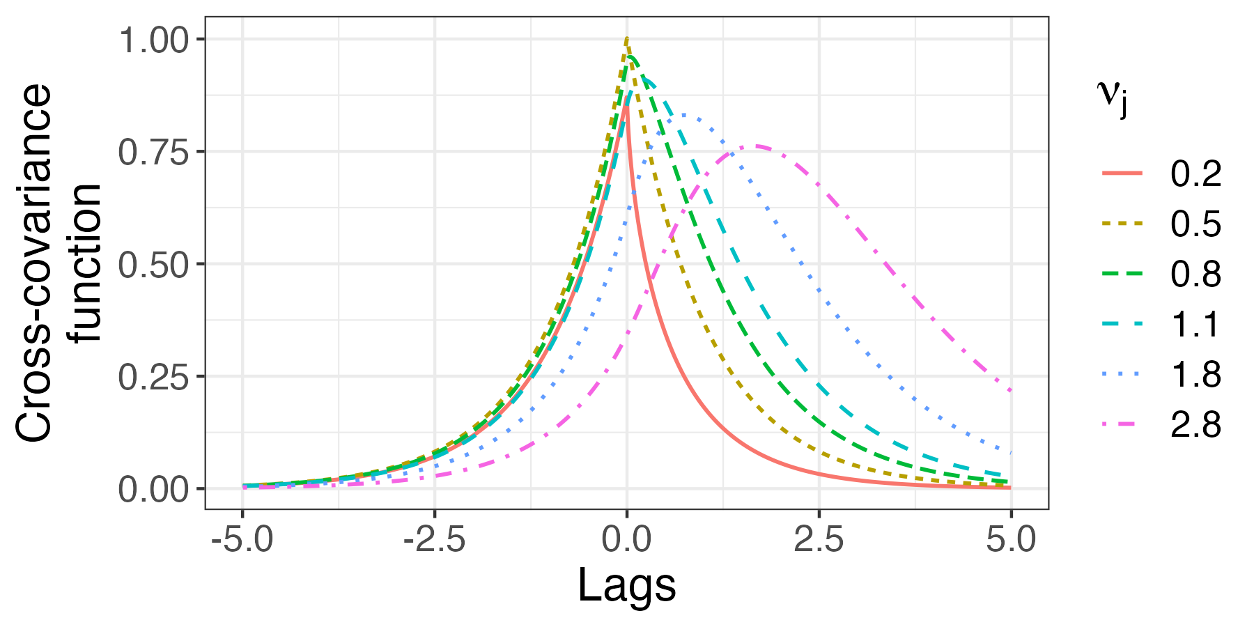
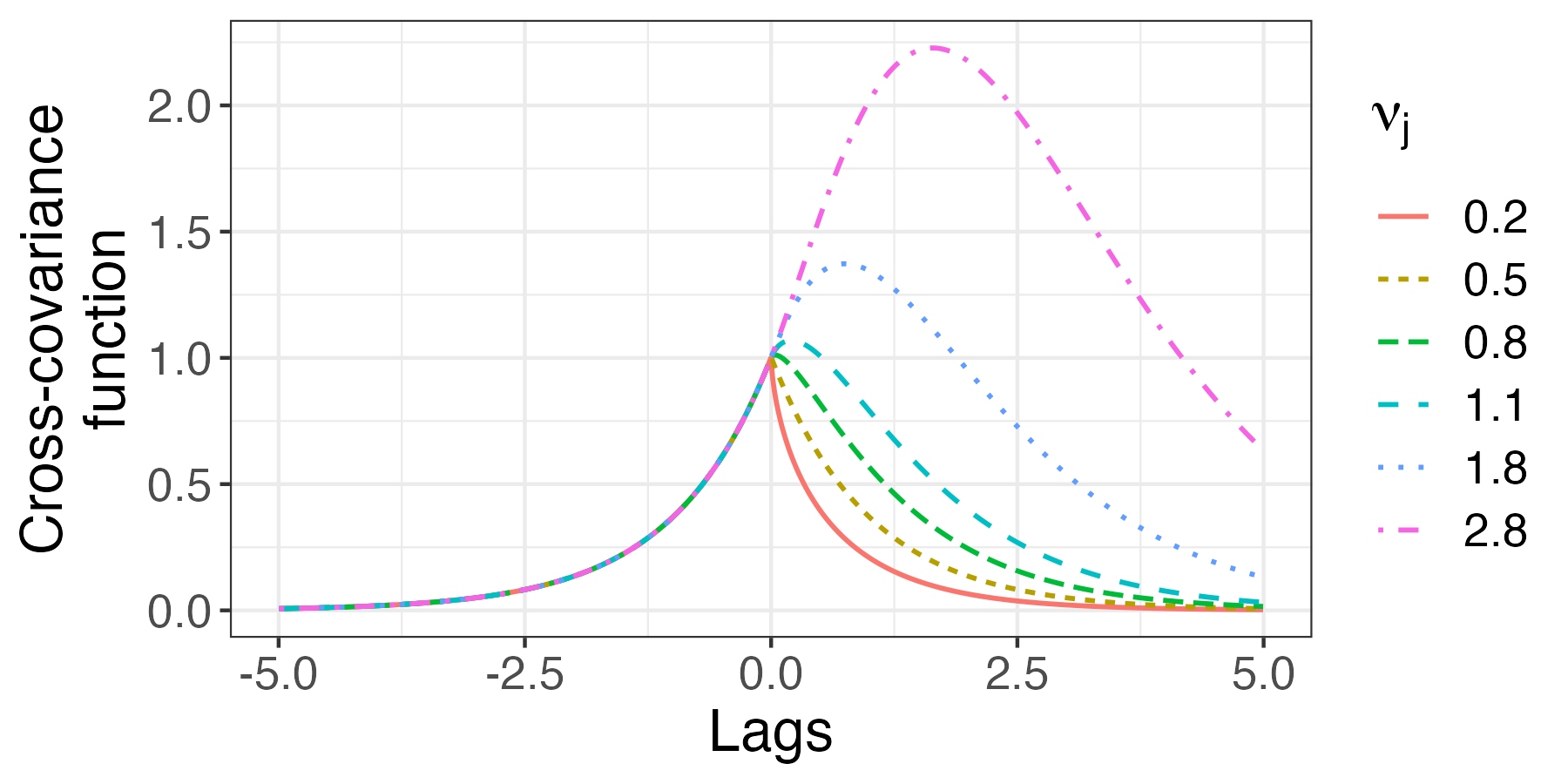
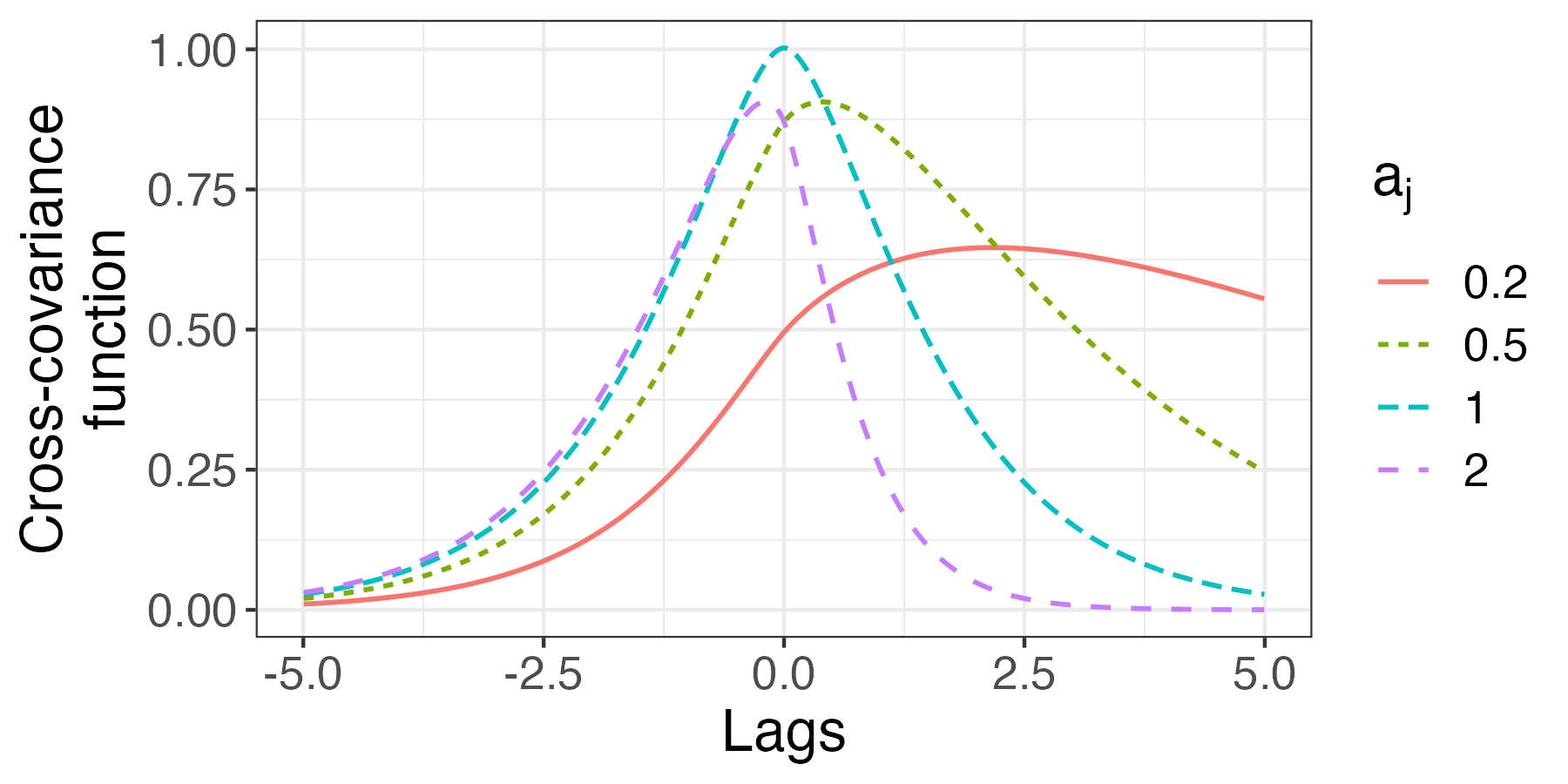
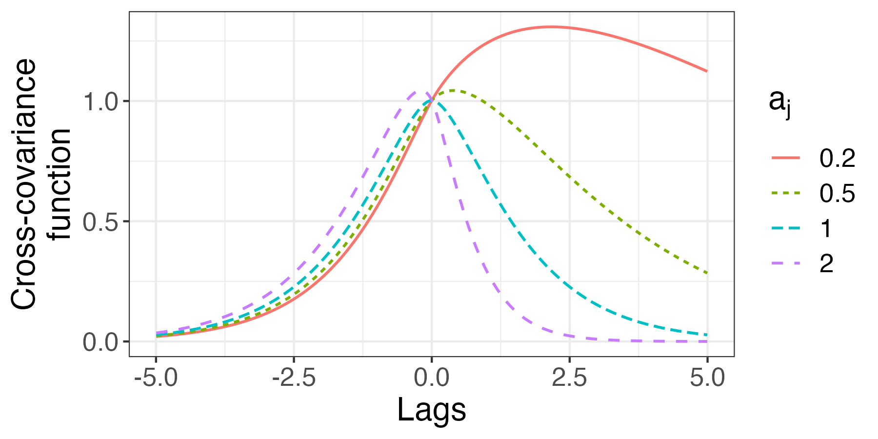
Figure 1: Matérn cross-covariances with $d=1$ and $\sigma_{jk}=1$ (Top) holding fixed $a_{j}=a_{k}=1$ and $\nu_{k}=0.5$, we plot the cross-covariance function when varying $\nu_{j}$ under (Upper Top) the original normalization and (Lower Top) the alternative normalization; (Bottom) Holding fixed $a_{k}=1$, $\nu_{j}=\nu_{k}=0.8$, we plot the cross-covariance function when varying $a_{j}$ under (Upper Bottom) the original normalization and (Lower Bottom) the alternative normalization.

Remark 3.6 (Expansion at $h\to\pm\infty$).

The asymptotic expression for the Matérn covariance is

$${\cal M}(|h|;a,\nu,\sigma_{11})\overset{h\to\infty}{\sim}\sigma_{11}\frac{2^{\frac{1}{2}-\nu}\sqrt{\pi}}{\Gamma(\nu)}(a|h|)^{\nu-\frac{1}{2}}\textrm{exp}(-a|h|),$$

by using the asymptotic expressions for the function $\mathcal{K}_{\nu}(z)\overset{z\to\infty}{\sim}(\pi/(2z))^{1/2}\textrm{exp}(-z)$ (see Section 10.40 of DLMF,, 2021). We will also use the asymptotic expansion of the function $W_{\kappa,\mu}(h)$ to analyze the asymptotic expression of the new cross-covariance (DLMF,, 2021). In particular, we combine (3.4) and (3.5) to obtain

$$C_{jk}(h)\overset{h\to\infty}{\sim}\Re(\sigma_{jk})c_{jk}^{*}(a_{j}|h|)^{\nu_{j}-\frac{1}{2}}\textrm{exp}(-a_{j}|h|),$$

so that, up to a positive constant that does not depend on $h$ defined by

$$c_{jk}^{*} =a_{j}^{\frac{1}{2}}a_{k}^{\nu_{k}}\sqrt{\frac{\Gamma(\nu_{k}+\frac{1}{2})}{\Gamma(\nu_{j}+\frac{1}{2})}}\frac{2\sqrt{\pi}(2\alpha_{+})^{-\nu_{k}-\frac{1}{2}}}{\sqrt{\Gamma(\nu_{j})\Gamma(\nu_{k})}},$$

the cross-covariance decays like the Matérn covariance class with parameters $\Re(\sigma_{jk})$, $\nu_{j}$, and $a_{j}$ in one direction. Of course, $\Re(\sigma_{jk})<0$ may hold to represent negative correlation between the two processes. Alternately, as $h\to-\infty$,

$$C_{jk}(h) \overset{h\to-\infty}{\sim}c^{*}_{kj}(a_{k}|h|)^{\nu_{k}-\frac{1}{2}}\textrm{exp}(-a_{k}|h|),$$

so that the cross-covariance decays (up to a constant) like the Matérn covariance class with parameters $\Re(\sigma_{jk})$, $\nu_{k}$, and $a_{k}$ in the other direction. Thus, the cross-covariance has the attractive property of reflecting the nature of the individual covariances when explaining the relationship between them; this relationship is also supported in Figure 1.

Remark 3.7 (Implementation).

The function $W_{\kappa,\nu}(z)$ is implemented as the whittakerW function in the R package fAsianOptions (Wuertz and Setz,, 2017), the mpmath.whitw function in Python, the whittakerW function in MatLab, and the WhittakerW function in Mathematica. Hančová et al., (2022) extensively evaluate computational infrastructure for computing (3.5) and related forms, though this computation is not always straightforward. For example, we find that the whittakerW function in the R package fAsianOptions does not give proper results when $\nu_{+}$ is a half-integer.

Remark 3.8 (Comparison).

A similar covariance function was studied in Section 5 of Lim and Eab, (2021) as a multifractional Ornstein-Uhlenbeck process. In particular, for a univariate process $X(s),s\in\mathbb{R}$, they let the exponent $\nu(s)>0$ be Hölder continuous with $|\nu(s_{1})-\nu(s_{2})|\leq\xi|s_{1}-s_{2}|^{\kappa}$ for constants $\xi>0$ and $\kappa>0$ and develop a covariance given by

$$\textrm{Cov}(X(s_{1}),X(s_{2}))=\frac{(s_{1}-s_{2})^{\nu_{+}(s_{1},s_{2})-\frac{1}{2}}}{\Gamma(\nu(s_{1})+\frac{1}{2})(2a)^{\nu_{+}(s_{1},s_{2})+\frac{1}{2}}}$$

$$~{}~{}~{}~{}~{}~{}~{}~{}~{}~{}\times W_{\nu_{-}(s_{1},s_{2}),\nu_{+}(s_{1},s_{2})}(2a(s_{1}-s_{2}))$$

for $\nu_{+}(s_{1},s_{2})=\frac{\nu(s_{1})+\nu(s_{2})}{2}$ and $\nu_{-}(s_{1},s_{2})=\frac{\nu(s_{1})-\nu(s_{2})}{2}$. Therefore, when $a=a_{j}=a_{k}$, the new Matérn cross-covariances are related to covariances of this multifractional Ornstein-Uhlenbeck process with varying parameter $\nu(s)$.

Remark 3.9 (Marginal cross-covariance).

One important quantity of interest for a cross-covariance function is the marginal cross-covariance between the processes, that is, $\mathbb{E}[Y_{j}(0)Y_{k}(0)]$. We have established the relation

$$C_{jk}(0) =\Re(\sigma_{jk})\frac{a_{j}^{\nu_{j}}a_{k}^{\nu_{k}}}{a_{+}^{2\nu_{+}}}\frac{\Gamma(2\nu_{+})}{\sqrt{\Gamma(2\nu_{j})\Gamma(2\nu_{k})}}.$$

When $a_{j}=a_{k}$ and $\nu_{j}=\nu_{k}$, we have the expected $C_{jk}(0)=\Re(\sigma_{jk})$. However, when $a_{j}\neq a_{k}$ or $\nu_{j}\neq\nu_{k}$, we instead have $C_{jk}(0)<\Re(\sigma_{jk})$. Intuitively, when the processes have different behavior, having high marginal correlation between them is challenging while maintaining the validity of the model. The model here adapts to this automatically, while the multivariate Matérn of Gneiting et al., (2010) initially allows $C_{jk}(0)=\Re(\sigma_{jk})$ for all parameter values yet then needs to further constrain possible values of $\Re(\sigma_{jk})$.

Remark 3.10 (Mode).

Hančová et al., (2022) suggest a numerical strategy in finding the mode of the probability density function of a gamma difference distribution using its derivative; in our case, the mode of the cross-correlation function corresponds to the lag of maximal absolute correlation between the two processes. Although a closed-form expression for the mode does not appear to be directly available, their approach may be applied here to find the lag and strength of maximal correlation between the processes.

By simplifying the model in $d=1$ to processes such that $\Im(\sigma_{jk})=0$, we provide a model that links two Matérn processes with a natural description of the cross-dependence. This new family of cross-covariance functions breaks the symmetry ($C_{jk}(h)=C_{jk}(-h)$) and diagonal-dominance ($\sup_{h}|C_{jk}(h)|=|C_{jk}(0)|$) assumptions of the multivariate Matérn of Gneiting et al., (2010) through imbalances between $\nu_{j}$ and $\nu_{k}$ or, alternatively, $a_{j}$ and $a_{k}$. It is only necessary to estimate one additional parameter, $\Re(\sigma_{jk})$, compared to estimating the parameters of the processes independently. Validity of the cross-covariance model is immediately available, and the model reduces to familiar models or forms for certain parameter values. These properties make this model for multivariate processes more attractive in multiple aspects compared to that of Gneiting et al., (2010) for the time-series setting.

3.2 Cross-covariances with imaginary directional measure

We now turn to cases where $\Im(\sigma_{jk})\neq 0$, which opens up an additional class of flexible cross-covariance functions. Here, we take the simplistic case when $\Re(\sigma_{jk})=0$, and then discuss the full model where $\Re(\sigma_{jk})\neq 0$ and $\Im(\sigma_{jk})\neq 0$ in Section 3.3. Notice that the value of $\Im(\sigma_{jk})$ is still constrained by the self-adjoint and positive properties of $\boldsymbol{\Sigma}_{H}$. For example, one must have $2|\Im(\sigma_{jk})|\leq\sigma_{jj}+\sigma_{kk}$.

Closed-form cross-covariances for such models have been challenging to find, yet we have had success in certain situations. One tool we will use is the Hilbert transform of a real function $C(h)$, which we define as

$${\cal H}[C](h) =\frac{1}{\pi}\int_{-\infty}^{\infty}\frac{C(u)}{h-u}du.$$ (3.6)

See King et al., (2018) for a comprehensive study of the Hilbert transform. Let $\mathcal{F}$ denote the Fourier transform (and $\mathcal{F}^{-1}$ its inverse), which is connected to the Hilbert transform by (King et al.,, 2018)

$$\mathcal{H}[C](h)=\mathcal{F}^{-1}[-\mathbbm{i}\textrm{sign}(\cdot)\mathcal{F}[C](\cdot)](h).$$

Using the notation of (3.2) and that $\mathcal{F}$ and $\mathcal{H}$ are linear, notice, then, that

$$C_{jk}^{\Im}(h) =-\mathcal{F}^{-1}[-\mathbbm{i}\textrm{sign}(\cdot)g_{jk}(\cdot)]=-\mathcal{H}[C_{jk}^{\Re}](h).$$

That is, the cross-covariances with purely imaginary directional measure are the negative Hilbert transform of the cross-covariances with real directional measure. Since a function and its Hilbert transform are orthogonal, we obtain that $\int_{\mathbb{R}}C_{jk}^{\Re}(h)C_{jk}^{\Im}(h)dh=0$. The component $C_{jk}^{\Im}(h)$ thus represents dependence that is fundamentally different or opposite of $C_{jk}^{\Re}(h)$, opening a new class of flexibility in the cross-covariance functions.

We first outline the cases for which we can find closed-form cross-covariances. We mention some functions that represent the cross-covariance for some values of the parameters. The modified Bessel function of the first kind is defined as

$$I_{\nu}(z) =\sum_{m=0}^{\infty}\frac{(\frac{1}{2}z)^{\nu+2m}}{\Gamma(m+1)\Gamma(\nu+m+1)}.$$ (3.7)

The modified Struve function of the first kind is defined as

$$L_{\nu}(z)=\sum_{m=0}^{\infty}\frac{(\frac{1}{2}z)^{2m+\nu+1}}{\Gamma(m+\frac{3}{2})\Gamma(m+\nu+\frac{3}{2})}.$$ (3.8)

See, for example, Section 3.7 of Watson, (1922) and Chapter 11 of DLMF, (2021) respectively for more information on these functions. We will also use the exponential integrals:

$$\textrm{E}_{1}(x) =\int_{1}^{\infty}\frac{e^{-tx}}{t}dt, \textrm{Ei}(x) =-\int_{-x}^{\infty}\frac{e^{-t}}{t}dt.$$

For $x>0$, the integral $\textrm{Ei}(x)$ is understood through the principal value.

Theorem 3.11.

Using the notation of (3.2), we have

$$C_{jk}^{\Im}(h)=-\mathcal{H}[C_{jk}^{\Re}](h),$$ (3.9)

where ${\cal H}$ stands for the Hilbert transform defined in (3.6).

In particular, assuming that $\Re(\sigma_{jk})=0$, for several important special cases, we obtain the following closed-form expressions of the cross-covariance:

1. Suppose that $\nu=\nu_{j}=\nu_{k}>0$ and $\nu\neq m/2$ for $m\in\mathbb{N}$, and $a=a_{j}=a_{k}>0$. Then, the cross-covariance function based on (1.9) is written in closed form as

   $$C_{jk}(h) =\Im(\sigma_{jk})\frac{\pi{\rm sign}(h)}{2\cos(\pi\nu)}\frac{2^{1-\nu}}{\Gamma(\nu)}\left(a|h|\right)^{\nu}$$

   $$~{}~{}~{}~{}~{}~{}~{}~{}~{}\times\left(L_{-\nu}(a|h|)-I_{\nu}(a|h|)\right).$$

2. Suppose that $\nu_{j}=\nu_{k}=1/2$, and let

   $$R(h,a_{j},a_{k})=\frac{-{\rm sign}(h)}{\pi}$$

   $$~{}~{}~{}\times\left(e^{a_{j}|h|}{E}_{1}(a_{j}|h|)+e^{-a_{k}|h|}{\rm Ei}(a_{k}|h|)\right).$$

   Then, the cross-covariance is written in closed form as

   $$C_{jk}(h) =\Im(\sigma_{jk})\frac{(a_{j}a_{k})^{\frac{1}{2}}}{a_{+}}(\mathbb{I}(h\leq 0)R(h,a_{j},a_{k})$$

   $$~{}~{}~{}~{}~{}~{}~{}~{}~{}~{}~{}~{}~{}~{}~{}~{}~{}~{}~{}~{}~{}~{}~{}~{}~{}~{}~{}~{}+\mathbb{I}(h>0)R(h,a_{k},a_{j})).$$

   Notice that if $a=a_{j}=a_{k}$, this reduces to $C_{jk}(h)=\Im(\sigma_{jk})R(h,a,a)$.

3. Suppose that $\nu_{j}=\nu_{k}=3/2$ and $a=a_{j}=a_{k}$. Then, the cross-covariance is written in closed form as

   $$C_{jk}(h) =\Im(\sigma_{jk})\Bigg{(}(a|h|+1)R(h,a,a)$$

   $$~{}~{}~{}~{}~{}~{}~{}~{}~{}~{}~{}~{}~{}~{}~{}~{}~{}~{}~{}~{}~{}~{}~{}~{}~{}~{}~{}-\frac{2ahe^{a|h|}}{\pi}{\rm Ei}(-a|h|)\Bigg{)}.$$

Proof.

Relation (3.9) has already been argued before the statement of the theorem.

We begin with the proof of Claim 1. The result for $\nu<1/2$ follows from the Hilbert transform of $|h|^{\nu}\mathcal{K}_{\nu}(a|h|)$ presented as (8I.2) in Table 1.8I of Appendix 1 of King, (2009). However, we present below the more general case that uses integral representations.

Focusing on $\Im(\sigma_{jk})\mathbbm{i}\int_{\mathbb{R}}e^{\mathbbm{i}hx}g_{jk}(x){\rm sign}(x)dx$, by substituting in $e^{\mathbbm{i}x}=\cos(x)+\mathbbm{i}\sin(x)$ and using even and odd properties of sine and cosine, we obtain

$$\begin{split}&\int_{\mathbb{R}}e^{\mathbbm{i}hx}g_{jk}(x)\textrm{sign}(x)dx\\ &=\int_{0}^{\infty}\cos(hx)g_{jk}(x)dx-\int_{0}^{\infty}\cos(hx)g_{jk}(-x)dx\\ &+\mathbbm{i}\int_{0}^{\infty}\sin(hx)g_{jk}(x)dx+\mathbbm{i}\int_{0}^{\infty}\sin(hx)g_{jk}(-x)dx.\end{split}$$

Since we assume here that $a_{j}=a_{k}$ and $\nu_{j}=\nu_{k}$, the function $g_{jk}(x)=g_{jk}(-x)$ is symmetric, and one sees that

$$\Im(\sigma_{jk})\mathbbm{i}\int_{\mathbb{R}}e^{\mathbbm{i}hx}g_{jk}(x){\rm sign}(x)dx$$

$$~{}~{}~{}~{}~{}~{}~{}=-2\Im(\sigma_{jk})\int_{0}^{\infty}\sin(hx)g_{jk}(x)dx.$$

Then, we adjust this expression to see

$$\mathbb{E}\left[Y_{j}(s+h)Y_{k}(s)\right]=-2\Im(\sigma_{jk})c_{j}^{2}\textrm{sign}(h)$$

$$~{}~{}~{}~{}~{}~{}~{}~{}~{}\times\int_{0}^{\infty}\sin(|h|x)\left(a^{2}+x^{2}\right)^{-\nu-\frac{1}{2}}dx,$$

since $(a+\mathbbm{i}x)^{-\nu-\frac{1}{2}}(a-\mathbbm{i}x)^{-\nu-\frac{1}{2}}=(a^{2}+x^{2})^{-\nu-\frac{1}{2}}$ and $c_{j}=c_{k}$. Then, we can directly apply 3.771 (1) of Gradshteyn et al., (2015), which also imposes the conditions on $\nu$. Particularly, we have a cross-covariance of

$$C_{jk}(h) =-\Im(\sigma_{jk})c_{j}^{2}\sqrt{\pi}\Gamma\left(\frac{1}{2}-\nu\right)\textrm{sign}(h)$$

$$~{}~{}~{}~{}~{}~{}~{}~{}~{}\times\left(\frac{|h|}{2a}\right)^{\nu}\left(I_{\nu}(a|h|)-L_{-\nu_{j}}(a|h|)\right)$$

when $\nu>0$ and $\nu\neq m/2$ for $m\in\mathbb{N}$.

Using Euler’s reflection formula for the Gamma function, we see

$$\Gamma\left(\frac{1}{2}-\nu\right)=\frac{\pi}{\Gamma\left(\frac{1}{2}+\nu\right)\cos(\pi\nu)}.$$

Subsequently substituting the value of $c_{j}$ gives the final expression.

To prove Claim 2, we use the Hilbert transform of $e^{-a|h|}$ given in (3.3) of Table 1.3 of Appendix 1 in King, (2009), which is $-R(h,a,a)$. When $a_{j}=a_{k}=a$, the result is immediate. For $a_{j}\neq a_{k}$, linearity of the Hilbert transforms can be used to find the Hilbert transform of the asymmetric Laplace function.

For Claim 3 where $\nu=3/2$ and $a=a_{j}=a_{k}$, since the Matérn covariance is $\sigma^{2}(1+a|h|)e^{-a|h|}$, we find the Hilbert transform of $|h|e^{-a|h|}$, which is $a|h|R(h,a,a)-2\pi^{-1}ahe^{a|h|}\textrm{Ei}(-a|h|)$. We defer the details to Section A. Combining the result with Claim 2 gives the final form.

∎

As before, we remark to provide more insight regarding those formulas in 1-3 above. In contrast to Theorem 3.1, we substitute in the value of $c_{j}$ and $c_{k}$, so that, for Claim 1, the form is similar to that of the Matérn covariance with a term of $2^{1-\nu}(a|h|)^{\nu}/\Gamma(\nu)$.

Remark 3.12 (Visualization and description).

In Figure 2, we plot the general shape of this cross-covariance function for varying $\nu=\nu_{j}=\nu_{k}$ and $a=a_{j}=a_{k}$. In this case, it is clear that the cross-covariance function is an odd function, so that the process $\{Y_{j}(s)\}$ may be positively correlated with process $\{Y_{k}(s)\}$ for some lags and negatively correlated for others. This also implies that two processes with this cross-covariance would be uncorrelated marginally in $s$. This is an interesting, unusual model, exhibiting a lack of marginal correlation as well as positive and negative dependence over non-zero lags. The cross-covariance appears to be an odd function only when $\nu=\nu_{j}=\nu_{k}$ and $a=a_{j}=a_{k}$, where the real and imaginary parts of the spectral density are analytically identifiable.

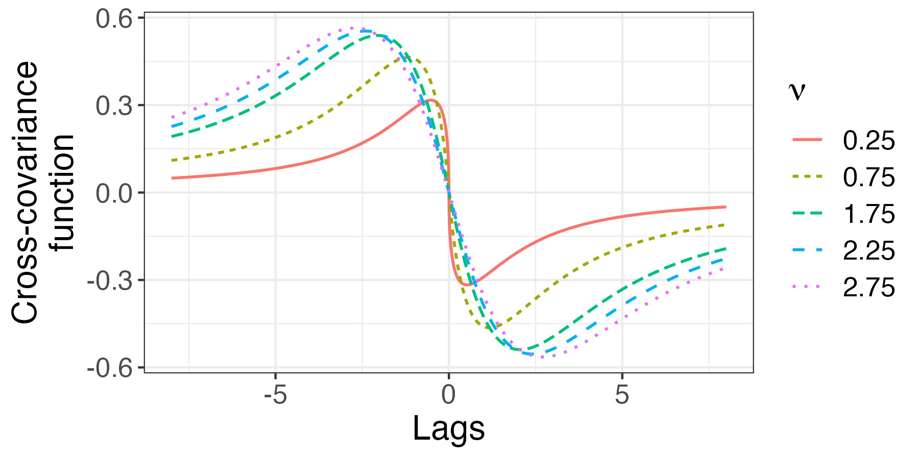
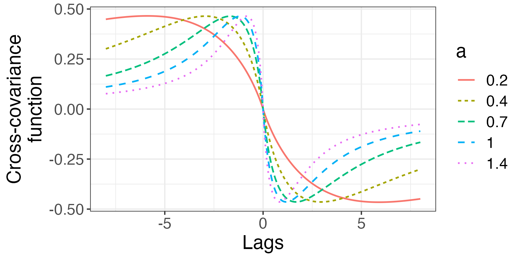
Figure 2: The cross-covariance function $C_{jk}(h)$ with $\sigma_{jk}=\mathbbm{i}$. (Top) With $a=a_{j}=a_{k}=1$ and various values of $\nu=\nu_{j}=\nu_{k}$. (Bottom) With $\nu=\nu_{j}=\nu_{k}=0.75$ and various values of $a=a_{j}=a_{k}$.

Remark 3.13 (Other cross-covariances when $\nu$ is a positive half-integer).

For $\nu_{j}=\nu_{k}=5/2,7/2,\dots$ and $a_{j}=a_{k}$, we expect that the cross-covariances can be found through tedious algebra involving Hilbert transforms, similar to the derivation for $\nu_{j}=\nu_{k}=3/2$ and $a_{j}=a_{k}$. These cross-covariances can be well-defined and computed as a limit as $\nu\to m/2$ or through the spectral density representation of the cross-covariance.

Remark 3.14.

Based on 12.2.6 of Abramowitz and Stegun, (1972), the asymptotic expression of

$$I_{\nu}(z)-L_{-\nu}(z)\overset{z\to\infty}{\sim}\frac{2^{\nu+1}}{\pi^{\frac{3}{2}}}\Gamma\left(\nu+\frac{1}{2}\right)z^{-\nu-1}\cos(\pi\nu)$$

holds. The asymptotic expansion for large $|h|$ of the cross-covariance is $\Im(\sigma_{jk})$ multiplied by

$$\begin{split}&\frac{\pi\textrm{sign}(h)}{2\cos(\pi\nu)}\frac{2^{1-\nu}}{\Gamma(\nu)}\left(a|h|\right)^{\nu}\left(L_{-\nu}(a|h|)-I_{\nu}(a|h|)\right)\\ &~{}~{}~{}~{}~{}\overset{|h|\to\infty}{\sim}\frac{-\textrm{sign}(h)2\Gamma(\nu+\frac{1}{2})}{\sqrt{\pi}\Gamma(\nu)a|h|}.\end{split}$$ (3.10)

The expansion suggests that the cross-covariance decays like $\Im(\sigma_{jk})\textrm{sign}(h)a^{-1}|h|^{-1}$, which is much larger in modulus compared to the Matérn covariance. This is surprising yet supported by our implementation (see Figure 2 as well as Figure 4 later).

For $\nu_{j}=\nu_{k}=1/2$, we use the asymptotic expansion of $E_{1}(h)\overset{h\to\infty}{\sim}e^{-h}/h$ and $\textrm{Ei}(h)\overset{h\to\infty}{\sim}e^{h}/h$ given in 6.12 of DLMF, (2021). We obtain

$$R(h,a_{j},a_{k})\overset{h\to\infty}{\sim}\frac{-1}{\pi}\left(\frac{1}{a_{j}h}+\frac{1}{a_{k}h}\right),$$

so that

$$C_{jk}(h)\overset{h\to\infty}{\sim}\Im(\sigma_{jk})\frac{2\sqrt{a_{j}a_{k}}}{(a_{j}+a_{k})}\frac{-1}{\pi}\left(\frac{1}{a_{j}h}+\frac{1}{a_{k}h}\right).$$

Notice that when $a_{j}=a_{k}$, we obtain the same formula suggested by (3.10) when $\nu=1/2$. In this case, the cross-covariance decays on the order of $1/(\min\{a_{j},a_{k}\}\cdot h)$ as $h\to\infty$. For $\nu_{j}=\nu_{k}=3/2$ and $a_{j}=a_{k}$, since $\textrm{Ei}(h)\overset{h\to-\infty}{\sim}e^{h}/h$, we obtain as expected

$$C_{jk}(h)\overset{h\to\infty}{\sim}\Im(\sigma_{jk})\frac{-4}{\pi ah}.$$

Remark 3.15 (Implementation).

The function $I_{\nu}(z)$ is implemented as besselI in the base package of R, iv in scipy in Python, besseli in Matlab, and besselI in Mathematica. The function $L_{\nu}(z)$ is implemented as struveL in the RandomFieldsUtils package of R (Schlather et al.,, 2022), modstruve in scipy in Python, and StruveL in Mathematica. We have also found using the series representation for $L_{-\nu}(z)$ in (3.8) works well for real-valued $\nu$ and $z$.

For $\textrm{Ei}(z)$ and $E_{1}(z)$, we use the expint package of R to compute its values (Goulet,, 2016).

When taking $\Im(\sigma_{jk})\neq 0$, we provide new closed-form Matérn cross-covariance functions in three different settings: when $a_{j}=a_{k}>0$ and $0<\nu_{j}=\nu_{k}\neq m/2$ for $m\in\mathbb{N}$; when $\nu_{j}=\nu_{k}=1/2$; and when $\nu_{j}=\nu_{k}=3/2$ and $a_{j}=a_{k}$. These functions greatly improve the flexibility of Matérn cross-covariances. As before, additional range and smoothness parameters do not need to be estimated.

The cross-covariances for other parameter settings are also of immediate interest. In Figure 3, we plot examples of these cross-covariances by using fast Fourier transform approaches with their spectral densities, demonstrating that such cross-covariances exist and have interpretable shapes as one varies the parameters. For example, it is apparent that changing $\nu_{j}$ and $a_{j}$ will significantly alter the shape of the cross-covariance function on one half of the real line while leaving the shape of the cross-covariance function relatively intact for the other half.

For the general case, closed-form expressions of the cross-covariances are more elusive. We suggest, however, that one consider the generalization of the functions $I_{\nu}(z)$ and $L_{\nu}(z)$ to the Whittaker function $M_{\mu,\nu}(z)$ and generalized modified Struve function $A_{\mu,\nu}(z)$, respectively; see Section 4.4 and Chapter 5 of Babister, (1967). However, it is unclear if the results there directly correspond to our setting for general $\nu_{j}$ and $\nu_{k}$. Furthermore, while the function $M_{\mu,\nu}(z)$ is well-documented, we are unaware of any sustained research, computational formula, or implementation of the function $A_{\mu,\nu}(z)$ for $\nu<0$. The form of the cross-covariance when $\nu_{j}=\nu_{k}$ and $a_{j}=a_{k}$ is also related closely to the modified Lommel function (see Equation 36 of Dingle,, 1959), but this relation does not appear to be helpful in generalizing the closed-form cross-covariance functions.

However, the spectral density represents these processes straightforwardly for general $\nu_{j}$, $\nu_{k}$, $a_{j}$, and $a_{k}$ even when closed-form representations are not available. Computationally, the values of the cross-covariance can be evaluated efficiently on a discrete grid of points using the fast Fourier transform (Cooley and Tukey,, 1965), which may be considerably faster than the evaluation of the relevant special functions.

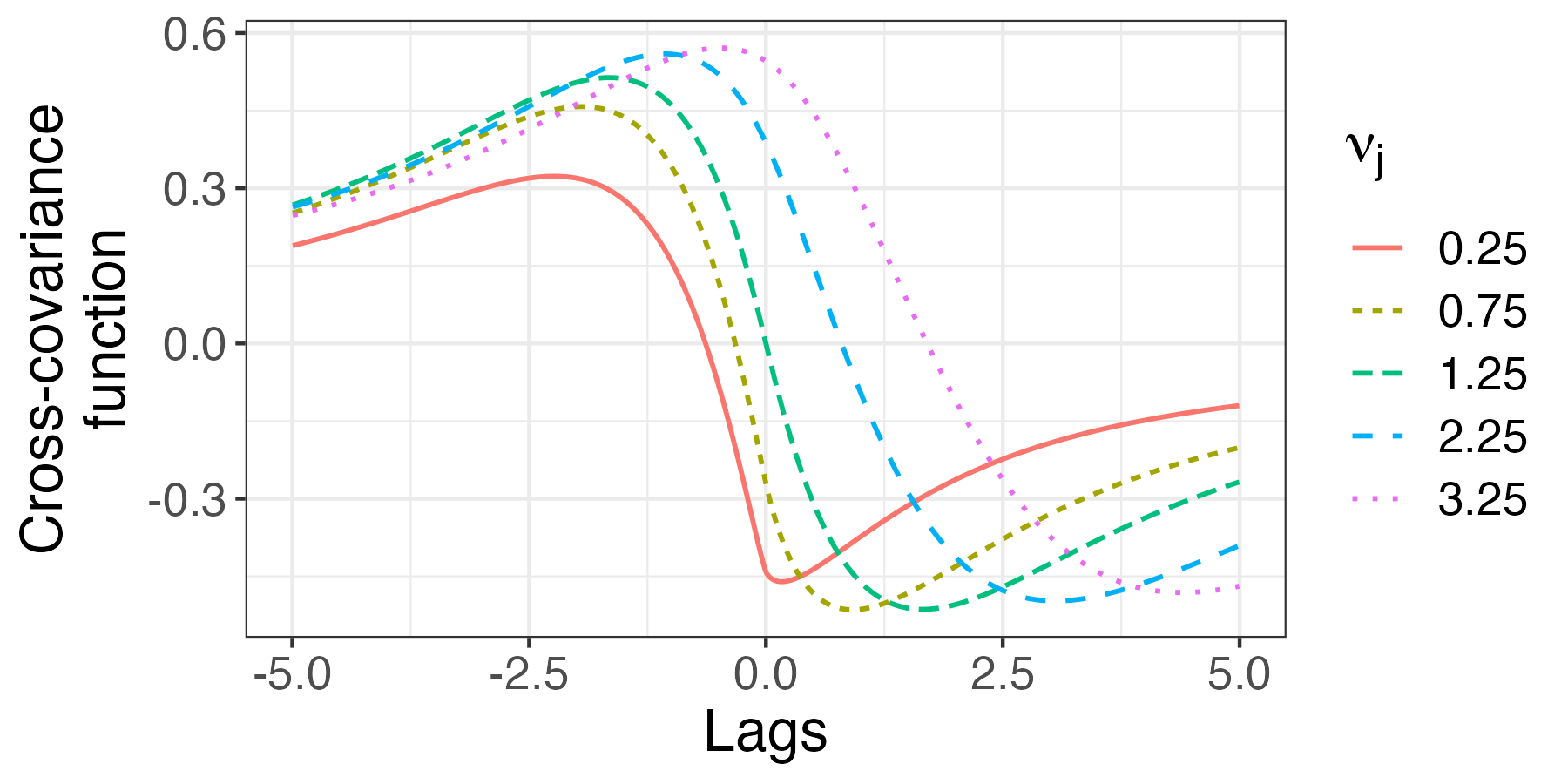
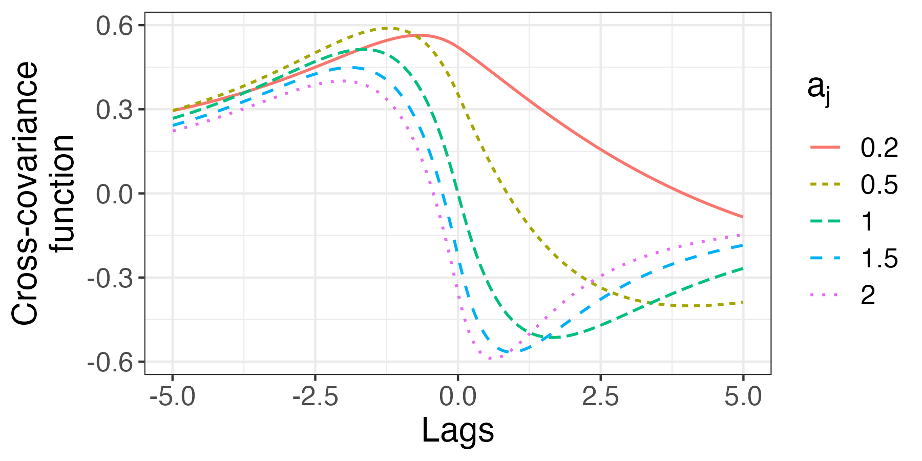
Figure 3: (Top) Multivariate Matérn cross-covariances with $a_{j}=a_{k}=1$, $\nu_{k}=1.25$, $\sigma_{jk}=\mathbbm{i}$, and $\nu_{j}$ varying. (Bottom) Multivariate Matérn cross-covariances with $a_{k}=1$, $\nu_{j}=\nu_{k}=1.25$, $\sigma_{jk}=\mathbbm{i}$, and $a_{j}$ varying.

3.3 Review of new multivariate Matérn models in one dimension

While in Theorem 3.1, we assume $\Im(\sigma_{jk})=0$, and in Theorem 3.11, we assume $\Re(\sigma_{jk})=0$, it is not necessary to have either be the case. If they are both nonzero, the cross-covariance is the sum of the respective contributions. Thus, to summarize, when $\boldsymbol{\Sigma}_{H}=[\sigma_{jk}]_{j,k=1}^{p}$ is positive definite and self-adjoint, we introduce a cross-covariance function represented by

$$\mathbb{E}[Y_{j}(h)Y_{k}(0)] =\Re(\sigma_{jk})C_{jk}^{\Re}(h)+\Im(\sigma_{jk})C_{jk}^{\Im}(h),$$

where, after substituting $c_{j}$ and $c_{k}$ into (3.5),

$$C_{jk}^{\Re}(h) =\frac{2^{-\nu_{+}}\sqrt{2\pi}}{\sqrt{\Gamma(\nu_{j})\Gamma(\nu_{k})}}\frac{a_{j}^{\nu_{j}}a_{k}^{\nu_{k}}}{a_{+}^{\nu_{+}+\frac{1}{2}}}|h|^{\nu_{+}-\frac{1}{2}}e^{-ha_{-}}$$

$$~{}~{}~{}~{}~{}\times\begin{cases}W_{\nu_{-},\nu_{+}}(2a_{+}|h|)\frac{\sqrt{\Gamma(\nu_{k}+\frac{1}{2})}}{\sqrt{\Gamma(\nu_{j}+\frac{1}{2})}}&h>0\\ W_{-\nu_{-},\nu_{+}}(2a_{+}|h|)\frac{\sqrt{\Gamma(\nu_{k}+\frac{1}{2})}}{\sqrt{\Gamma(\nu_{j}+\frac{1}{2})}}&h<0\end{cases}.$$

We refer to $C_{jk}^{\Im}(h)$, which is available in integral form, as an extended Matérn cross-correlation function for $d=1$. Such combinations provide a large class of potential shapes in the cross-covariance functions, with examples shown in Figure 4. In the specific case where $\nu=\nu_{j}=\nu_{k}\neq m/2$ for $m\in\mathbb{N}$ and $a=a_{j}=a_{k}$, the cross-covariance function becomes

$$\mathbb{E}[Y_{j}(h)Y_{k}(0)]=\frac{2^{1-\nu}}{\Gamma(\nu)}(a|h|)^{\nu}\Bigg{(}\Re(\sigma_{jk})\mathcal{K}_{\nu}(a|h|)$$

$$~{}~{}~{}~{}~{}+\Im(\sigma_{jk})\frac{\pi\textrm{sign}(h)}{2\cos(\pi\nu)}(L_{-\nu}(a|h|)-I_{\nu}(a|h|))\Bigg{)},$$

which is decomposed as a sum of an even and an odd function. In the special case that $\nu_{j}=\nu_{k}=1/2$, we obtain

$$\mathbb{E}[Y_{j}(h)Y_{k}(0)]=\frac{2(a_{j}a_{k})^{\frac{1}{2}}}{a_{j}+a_{k}}$$

$$\times[\Re(\sigma_{jk})\textrm{exp}\left(-|h|(a_{j}\mathbb{I}(h>0)+a_{k}\mathbb{I}(h<0))\right)$$

$$+\Im(\sigma_{jk})\left(\mathbb{I}(h\leq 0)R(h,a_{j},a_{k})+\mathbb{I}(h>0)R(h,a_{k},a_{j})\right)].$$

In Figure 5, we plot realizations of the multivariate Matérn process for two different parameter settings. For two processes with different smoothness and real-valued $\sigma_{jk}$, one can easily pick out correlation between the processes; however, when $\sigma_{jk}$ is imaginary-valued, the dependence between the processes is harder to pick out visually since the processes are uncorrelated marginally.

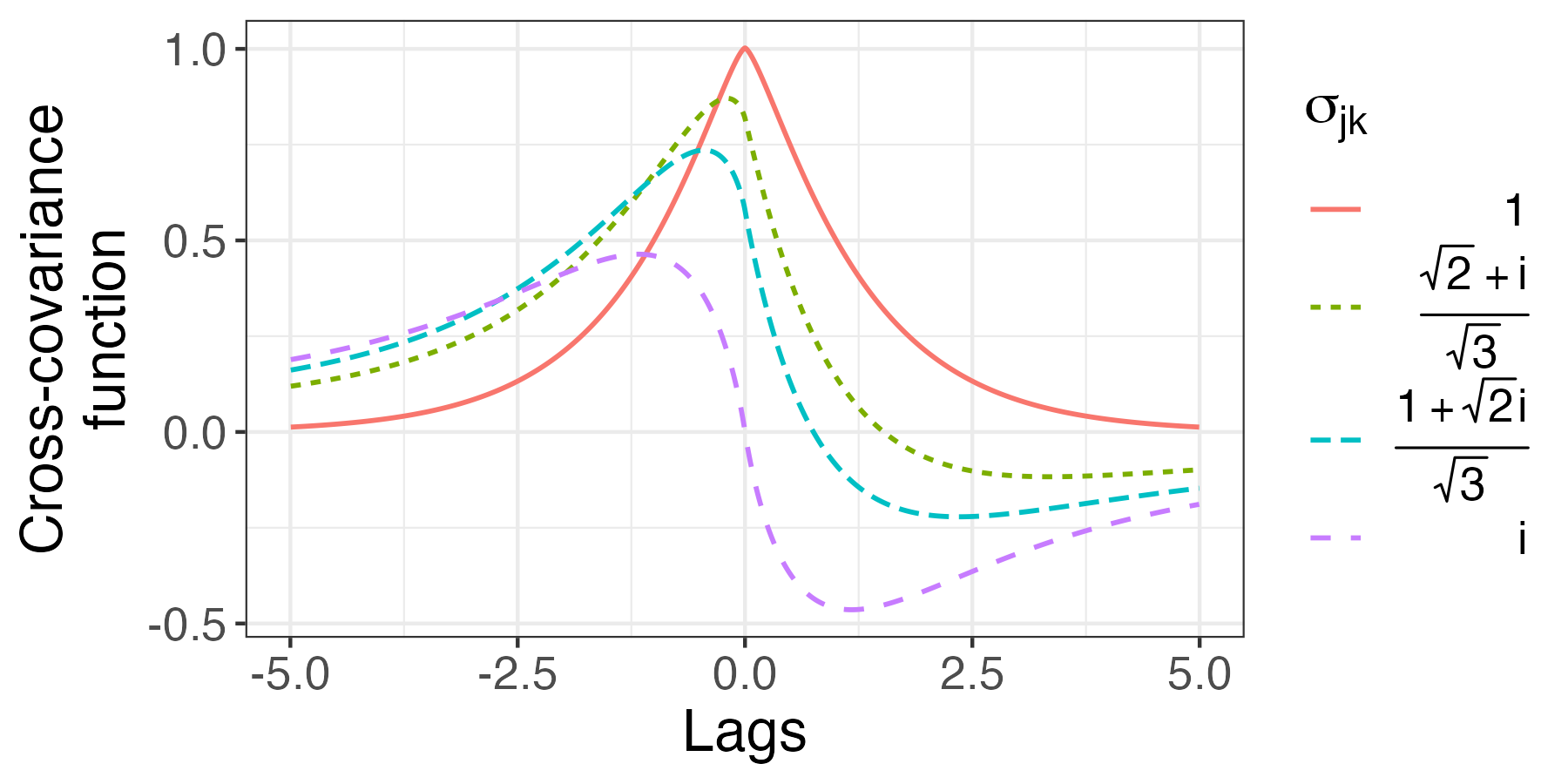
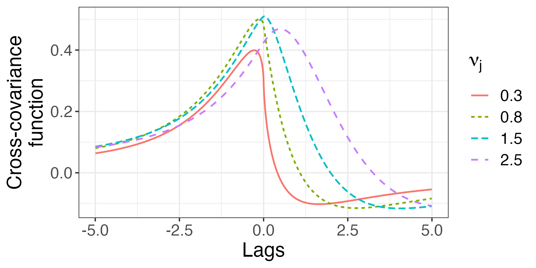
Figure 4: (Top) Multivariate Matérn cross-covariances for varying values of $\sigma_{jk}$, with $d=1$, $\nu_{j}=\nu_{k}=0.75$, and $a_{j}=a_{k}=1$. (Bottom) Multivariate Matérn cross-covariances for varying values of $\nu_{j}$, with $d=1$, $\sigma_{jk}=0.5+0.4\mathbbm{i}$, $\nu_{k}=0.5$, and $a_{j}=a_{k}=1$.

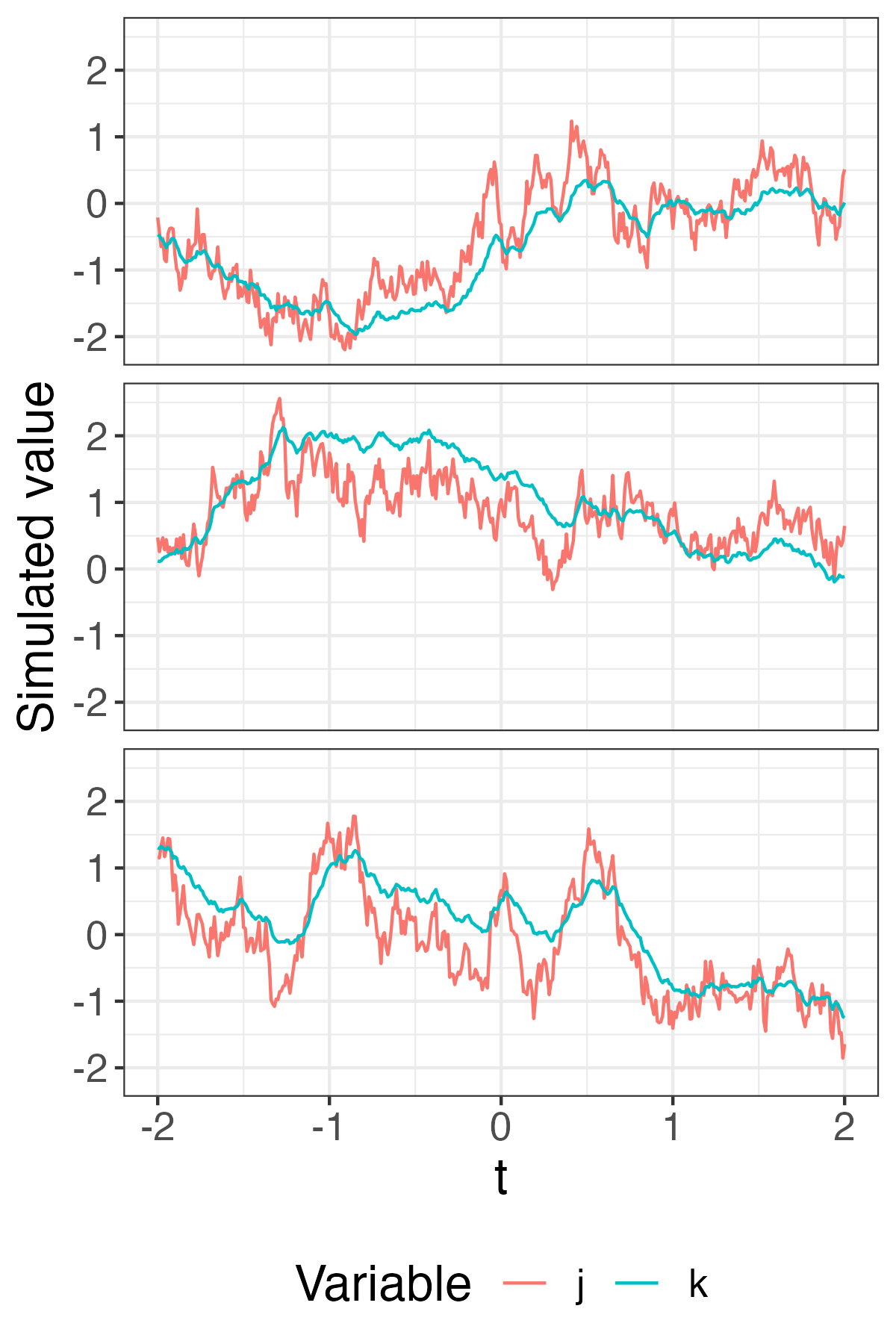
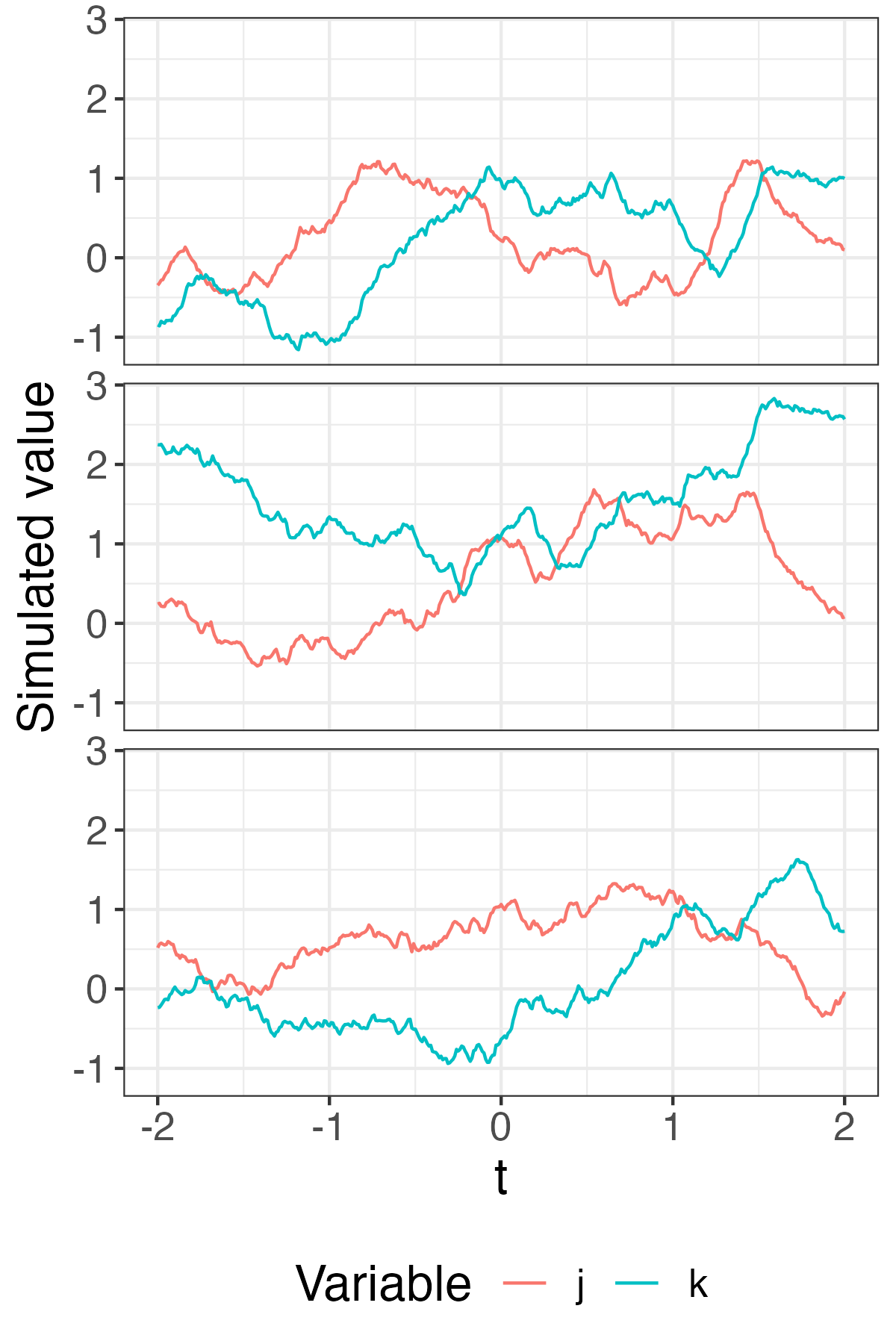
Figure 5: Three realizations of bivariate Matérn processes for $d=1$, with $a_{j}=a_{k}=1$ and $\sigma_{jj}=\sigma_{kk}=1$. (Left) For $\nu_{j}=0.4$, $\nu_{k}=0.8$, and $\sigma_{jk}=0.95$. (Right) For $\nu_{j}=\nu_{k}=0.8$ and $\sigma_{jk}=-0.95\mathbbm{i}$.

4 Spatial extensions of multivariate Matérn models

In this section, we will extend our approach to the random field setting, i.e., to processes indexed by $\mathbb{R}^{d}$ for $d\geq 2$. The spatial setting calls for substantially more flexible models that can accommodate anisotropy. For a general outlook and the motivation of our approach from the perspective of tangent processes, see Section E. Here, we will directly describe the model.

In the spatial setting, it is more convenient to consider integration in polar coordinates. Namely, for $\boldsymbol{s}\in\mathbb{R}^{d}\setminus\{\boldsymbol{0}\}$, we let $r=\|\boldsymbol{s}\|$ and $\boldsymbol{\theta}:=\boldsymbol{s}/\|\boldsymbol{s}\|$, so that $\boldsymbol{s}$ is represented with the pair of its radial and directional components $(r,\boldsymbol{\theta})\in(0,\infty)\times\mathcal{S}^{d-1}$, where $\mathcal{S}^{d-1}$ denotes the unit sphere in $\mathbb{R}^{d}$.

Also, we will use matrix exponentiation and powers to describe our integrands. For all $c>0$, we let $c^{\boldsymbol{H}}:=\exp\{\log(c)\boldsymbol{H}\}$, where, for a square matrix $\boldsymbol{A}$, its exponential $\exp\{\boldsymbol{A}\}$ is defined as:

$$e^{\boldsymbol{A}}=\sum_{n=0}^{\infty}\frac{\boldsymbol{A}^{n}}{n!}.$$

Note that the latter series converges absolutely in any matrix norm. We will further use the definition of $\boldsymbol{A}^{\boldsymbol{B}}$ for two matrices of equal size as ${\rm exp}(\log(\boldsymbol{A})\boldsymbol{B})$, whenever the matrix logarithm is well-defined. One can use, for example, the Gregory series

$$\log(\boldsymbol{A})=\sum_{n=0}^{\infty}\frac{-2}{2n+1}\Big{(}(\boldsymbol{I}-\boldsymbol{A})(\boldsymbol{I}+\boldsymbol{A})^{-1}\Big{)}^{2n+1},$$ (4.1)

which is convergent provided that the eigenvalues of $\boldsymbol{A}$ have positive real parts (cf. Higham,, 2008; Cardoso and Sadeghi,, 2018; Barradas and Cohen,, 1994). In most cases, we will apply this to a diagonal matrix $\boldsymbol{A}=\textrm{diag}(\lambda_{1},\lambda_{2},\dots,\lambda_{p})$, in which case we have the expansion

$$\log(\boldsymbol{A}) =\textrm{diag}\left(\sum_{n=0}^{\infty}\frac{-2}{2n+1}\left[\frac{1-\lambda_{j}}{1+\lambda_{j}}\right]^{2n+1},j=1,\dots,p\right)$$

$$=\textrm{diag}\left(\log(\lambda_{j}),j=1,\dots,p\right).$$

We will then define matrix versions of the parameters. First, define a diagonal matrix of inverse range parameters as $\boldsymbol{a}=\textrm{diag}(a_{1},\dots,a_{p})$, and similarly take $\boldsymbol{c}=\textrm{diag}(c_{1},\dots,c_{p})$ for normalization constants $c_{j}>0$; we will extend their definitions for general $d$ later. Let $\boldsymbol{\nu}=\textrm{diag}(\nu_{1},\dots,\nu_{p})$ for positive $\nu_{j}$. Finally, let $\boldsymbol{I}_{d}$ again be the identity matrix of dimension $d\times d$.

Remark 4.1.

One may also consider the more general case for $\boldsymbol{\nu}$. For example, if $\boldsymbol{\nu}$ and $\boldsymbol{a}$ commute, the definition below may be straightforwardly applicable to where $\boldsymbol{\nu}\in\mathbb{R}^{p\times p}$ is a real, symmetric, positive-definite matrix that is potentially non-diagonal. One case that accommodates this more-flexible $\boldsymbol{\nu}$ (and perhaps the only notable case) is where $\boldsymbol{a}=a\boldsymbol{I}_{p}$ for $a>0$.

Following Definitions 2.4 and 2.7, let $\boldsymbol{B}_{\boldsymbol{\mu}}(dr,d\boldsymbol{\theta})$ be a Hermitian zero-mean $\mathbb{C}^{p}$-valued random measure, with orthogonal increments that satisfies:

$$\mathbb{E}\left[\boldsymbol{B}_{\boldsymbol{\mu}}(dr,d\boldsymbol{\theta})\boldsymbol{B}_{\boldsymbol{\mu}}(dr,d\boldsymbol{\theta})^{*}\right] =r^{d-1}dr\boldsymbol{\mu}(d\boldsymbol{\theta}).$$ (4.2)

For concreteness, we take $\boldsymbol{B}_{\boldsymbol{\mu}}(dr,d\boldsymbol{\theta})$ to be Gaussian, but many other choices are possible leading to further flexibility in the models. Here, the control measure $\boldsymbol{\mu}(d\boldsymbol{\theta})$ is a $\mathbb{T}_{+}$-valued measure on $\mathcal{S}^{d-1}$, which is also Hermitian, i.e., such that $\boldsymbol{\mu}(d\boldsymbol{\theta})=\overline{\boldsymbol{\mu}(-d\boldsymbol{\theta})}$ (cf. Definition 2.7). This generalizes the measure $\boldsymbol{\mu}(dx)$ used in Section 1. Furthermore, we take $\boldsymbol{\mu}(d\boldsymbol{\theta})$ to be finite so that $\left\lVert\boldsymbol{\mu}(\mathcal{S}^{d-1})\right\rVert_{F}<\infty$ for the Frobenius norm $\lVert\cdot\rVert_{F}$.

4.1 Proposed model

We propose to study the multivariate Matérn process generated by

$$\begin{split}&\{\boldsymbol{Y}(\boldsymbol{s})\}_{\boldsymbol{s}\in\mathbb{R}^{d}}\overset{fdd}{=}\Bigg{\{}\int_{0}^{\infty}\int_{\mathcal{S}^{d-1}}e^{\mathbbm{i}\langle\boldsymbol{s},r\boldsymbol{\theta}\rangle}\\ &~{}~{}\times\boldsymbol{c}(\boldsymbol{a}+\varphi(\boldsymbol{\theta})\mathbbm{i}r\boldsymbol{I}_{p})^{-\boldsymbol{\nu}-\frac{d}{2}\boldsymbol{I}_{p}}\boldsymbol{B}_{\boldsymbol{\mu}}(dr,d\boldsymbol{\theta})\Bigg{\}}_{\boldsymbol{s}\in\mathbb{R}^{d}}.\end{split}$$ (4.3)

We provide more details about the representation of (4.3) and introduce the function $\varphi:\mathcal{S}^{d-1}\to\{-1,1\}$. The matrix $\boldsymbol{\nu}$ essentially corresponds to the smoothness of the Matérn processes. Under the assumption of diagonal $\boldsymbol{\nu}$ and $\boldsymbol{c}$, working with the exponential and logarithm definitions, we see that

$$\boldsymbol{c}(\boldsymbol{a}+\varphi(\boldsymbol{\theta})\mathbbm{i}r\boldsymbol{I}_{p})^{-\boldsymbol{\nu}-\frac{d}{2}\boldsymbol{I}_{p}}$$

$$~{}~{}~{}~{}~{}=\textrm{diag}\left(c_{k}(a_{k}+\varphi(\boldsymbol{\theta})\mathbbm{i}r)^{-\nu_{k}-\frac{d}{2}},k=1,\dots,p\right),$$

which will simplify our analysis. We take $\varphi:\mathcal{S}^{d-1}\to\{-1,1\}$ to be a function such that $\varphi(-\boldsymbol{\theta})=-\varphi(\boldsymbol{\theta})$. The function $\varphi(\cdot)$ ensures that the spectral density in (4.3) is Hermitian and the cross-covariances are real (cf. Proposition 2.6 and Definition 2.7).

Remark 4.2.

In the case $d=1$, the above model reduces to the one we have already introduced in Section 3. Indeed, in this case $\mathcal{S}^{d-1}=\mathcal{S}^{0}=\{-1,1\}$, and the only two possible Hermitian functions are $\varphi({\theta})=\pm\textrm{sign}({\theta})$. Then, $\boldsymbol{\mu}(d\theta)=\Re(\boldsymbol{\Sigma}_{H})+\mathbbm{i}\Im(\boldsymbol{\Sigma}_{H})\textrm{sign}({\theta})d\theta$, where $\boldsymbol{\Sigma}_{H}=[\sigma_{jk}]_{j,k=1}^{p}$. If $\boldsymbol{\nu}$ is also diagonal and we take $\varphi({\theta})=\textrm{sign}({\theta})$, this results in cross-covariances of

$$C_{jk}(h)=c_{j}c_{k}\int_{0}^{\infty}\int_{\mathcal{S}^{0}}e^{\mathbbm{i}hr}(a_{j}+\textrm{sign}({\theta})\mathbbm{i}r)^{-\nu_{j}-\frac{1}{2}}$$

$$~{}~{}~{}~{}~{}\times\left(\Re(\sigma_{jk})+\mathbbm{i}\Im(\sigma_{jk})\textrm{sign}({\theta})\right)$$

$$~{}~{}~{}~{}~{}\times(a_{k}-\textrm{sign}({\theta})\mathbbm{i}r)^{-\nu_{k}-\frac{1}{2}}d\theta dr$$

$$~{}~{}~{}~{}~{}~{}~{}~{}~{}~{}~{}~{}=c_{j}c_{k}\int_{-\infty}^{\infty}e^{\mathbbm{i}hr}(a_{j}+\mathbbm{i}r)^{-\nu_{j}-\frac{1}{2}}$$

$$~{}~{}~{}~{}~{}\times\left(\Re(\sigma_{jk})+\mathbbm{i}\Im(\sigma_{jk})\textrm{sign}(r)\right)(a_{k}-\mathbbm{i}r)^{-\nu_{k}-\frac{1}{2}}dr,$$

which recovers the representation in (3.1) where the integral is in Cartesian coordinates on $\mathbb{R}$. When $\varphi(\theta)=-\textrm{sign}(\theta)$, we obtain reversed versions of the covariances (cf. Proposition D.3).

We next demonstrate that the marginal processes of $\boldsymbol{Y}(\boldsymbol{s})$ are Matérn for a certain choice for $\boldsymbol{\mu}(d\boldsymbol{\theta})$. Here and throughout, let $d\boldsymbol{\theta}$ represent the uniform probability distribution on $\mathcal{S}^{d-1}$.

Proposition 4.3.

Suppose the diagonal of $\boldsymbol{\mu}(d\boldsymbol{\theta})$ has constant spectral density with respect to $d\boldsymbol{\theta}$. That is,

$${\textrm{diag}}(\boldsymbol{\mu}(d\boldsymbol{\theta}))=\left[\sigma_{11}d\boldsymbol{\theta},\sigma_{22}d\boldsymbol{\theta},\cdots,\sigma_{pp}d\boldsymbol{\theta}\right]$$

for $\sigma_{jj}>0$. Define the normalization constants as

$$c_{j}=\frac{a_{j}^{\nu_{j}}\sqrt{\Gamma(\nu_{j}+\frac{d}{2})}}{\pi^{\frac{d}{4}}\sqrt{\Gamma(\nu_{j})}},$$ (4.4)

and let $\boldsymbol{Y}(\boldsymbol{s}):=(Y_{j}(\boldsymbol{s}))_{j=1}^{p},\ \boldsymbol{s}\in\mathbb{R}^{d}$ be the multivariate Matérn process given by (4.3). Then, for each $j=1,\cdots,p$, the marginal process $\{Y_{j}(\boldsymbol{s})\}$ has the Matérn covariance functions with inverse range parameter $a_{j}$, smoothness parameters $\nu_{j}$, and variance parameters $\sigma_{jj}$.

Proof.

Writing $\boldsymbol{\mu}(d\boldsymbol{\theta})=[\mu_{jk}(d\boldsymbol{\theta})]_{j=1,k=1}^{p}$, we see

$$C_{jj}(\boldsymbol{h})=c_{j}^{2}\int_{0}^{\infty}\int_{\mathcal{S}^{d-1}}e^{\mathbbm{i}\langle\boldsymbol{h},r\boldsymbol{\theta}\rangle}\left(a_{j}+\varphi(\boldsymbol{\theta})\mathbbm{i}r\right)^{-\nu_{j}-\frac{d}{2}}$$

$$~{}~{}~{}~{}~{}~{}~{}~{}\times\mu_{jj}(d\boldsymbol{\theta})\left(a_{j}-\varphi(\boldsymbol{\theta})\mathbbm{i}r\right)^{-\nu_{j}-\frac{d}{2}}dr$$

$$=c_{j}^{2}\sigma_{jj}\int_{0}^{\infty}\int_{\mathcal{S}^{d-1}}e^{\mathbbm{i}\langle\boldsymbol{h},r\boldsymbol{\theta}\rangle}\left(a_{j}^{2}+r^{2}\right)^{-\nu_{j}-\frac{d}{2}}r^{d-1}d\boldsymbol{\theta}dr$$

since $(a+b\mathbbm{i})^{d}(a-b\mathbbm{i})^{d}=\left(a^{2}+b^{2}\right)^{d}$ and $\varphi(\boldsymbol{\theta})^{2}=1$. Define the Bessel function (see Watson,, 1922) as

$$J_{\nu}(z)=\sum_{m=0}^{\infty}\frac{(-1)^{m}}{\Gamma(m+1)\Gamma(m+\nu+1)}\left(\frac{z}{2}\right)^{2m+\nu}.$$

We next use the representation of the Bessel function and the inversion formula on page 43 and 46, respectively, of Stein, (1999) to obtain

$$\begin{split}&C_{jj}(\boldsymbol{h})=c_{j}^{2}(2\pi)^{\frac{d}{2}}\sigma_{jj}\left\lVert\boldsymbol{h}\right\rVert^{\frac{-d+2}{2}}\\ &~{}~{}~{}~{}~{}\times\int_{0}^{\infty}J_{(d-2)/2}(r\left\lVert\boldsymbol{h}\right\rVert)\left(a_{j}^{2}+r^{2}\right)^{-\nu_{j}-\frac{d}{2}}r^{\frac{d}{2}}dx.\end{split}$$ (4.5)

Thus, the Fourier transform on $\mathbb{R}^{d}$ reduces to the Hankel transform (involving the Bessel function $J_{\nu}(z)$) on $\mathbb{R}$. The representation (4.5) is proportional to the Matérn covariance in (1.4); see the representation of the Matérn spectral density on page 49 of Stein, (1999).

Formally showing this, we use 6.565 (4) of Gradshteyn et al., (2015) to obtain

$$C_{jj}(\boldsymbol{h}) =c_{j}^{2}2^{1-\nu_{j}}\pi^{\frac{d}{2}}\sigma_{jj}\left\lVert\boldsymbol{h}\right\rVert^{\nu_{j}}\frac{a_{j}^{-\nu_{j}}}{\Gamma(\nu_{j}+\frac{d}{2})}\mathcal{K}_{\nu_{j}}(a_{j}\left\lVert\boldsymbol{h}\right\rVert).$$

Then, using the expression $\mathcal{K}_{\nu}(z)\sim 2^{-1}\Gamma(\nu)(z/2)^{-\nu},$ as $z\to 0$ (see Section 10.30 of DLMF,, 2021), we see

$$C_{jj}(\boldsymbol{0}) =c_{j}^{2}\pi^{\frac{d}{2}}\sigma_{jj}\frac{\Gamma(\nu_{j})}{a_{j}^{2\nu_{j}}\Gamma(\nu_{j}+\frac{d}{2})}.$$

Therefore, from our choice of $c_{j}$, we obtain $C_{jj}(\boldsymbol{0})=\sigma_{jj}$ and

$$C_{jj}(\boldsymbol{h}) =\sigma_{jj}\frac{2^{1-\nu_{j}}}{\Gamma(\nu_{j})}\left(a_{j}\left\lVert\boldsymbol{h}\right\rVert\right)^{\nu_{j}}\mathcal{K}_{\nu_{j}}(a_{j}\left\lVert\boldsymbol{h}\right\rVert)$$

$$=\mathcal{M}(\lVert\boldsymbol{h}\rVert;a_{j},\nu_{j},\sigma_{jj}).$$

This completes the proof. ∎

The Matérn-type model defined in (4.3) depends on the choice of the directional measure $\boldsymbol{\mu}(d\boldsymbol{\theta})$. This, in the spatial setting $(d\geq 2)$ leads to a great amount of flexibility, since $\boldsymbol{\mu}(d\boldsymbol{\theta})$ is in fact an infinite-dimensional parameter. Therefore, in contrast to the case $d=1$, one cannot expect to obtain a canonical “spatial extension” of the classical Matérn model even in the scalar-valued regime $p=1$. In what follows, we will offer several natural approaches, where we begin with more basic models for $\boldsymbol{\mu}(d\boldsymbol{\theta})$ and then gradually build more complexity in the model.

Since the integrals above are not often available in closed form for most parameter settings, we approximate the integrals for the plots in this section, and Fourier transform approaches can be used to do this quickly (Averbuch et al.,, 2006). Furthermore, the processes can be simulated efficiently. Throughout this section, we use the simulation approach of Emery et al., (2016) as recommended in Alegría et al., (2021), which uses the spectral density and a form of importance sampling to simulate the multivariate process.

4.2 Cross-covariances with real directional measure

Here, we consider the case where $\boldsymbol{\mu}(d\boldsymbol{\theta})=\boldsymbol{\Sigma}d\boldsymbol{\theta}$ for some self-adjoint and positive-definite matrix $\boldsymbol{\Sigma}=[\sigma_{jk}]_{j,k=1}^{p}$. In contrast to $\boldsymbol{\Sigma}_{H}$ of Section 3, the matrix $\boldsymbol{\Sigma}$ must be a real-valued matrix in this case, due to the requirement $\boldsymbol{\mu}(d\boldsymbol{\theta})=\overline{\boldsymbol{\mu}(-d\boldsymbol{\theta})}$. In this setting, we obtain a cross-covariance of

$$C_{jk}(\boldsymbol{h})=\sigma_{jk}c_{j}c_{k}\int_{-\infty}^{\infty}\int_{\mathcal{S}^{d-1},\varphi(\boldsymbol{\theta})=1}e^{\mathbbm{i}\langle\boldsymbol{h},r\boldsymbol{\theta}\rangle}$$

$$~{}~{}~{}~{}~{}~{}~{}\times\left(a_{j}+\mathbbm{i}r\right)^{-\nu_{j}-\frac{d}{2}}\left(a_{k}-\mathbbm{i}r\right)^{-\nu_{k}-\frac{d}{2}}|r|^{d-1}d\boldsymbol{\theta}dr.$$

This integral can be somewhat simplified if one assumes that $\{\boldsymbol{\theta}|\varphi(\boldsymbol{\theta})=1\}=\{\boldsymbol{\theta}|\langle\boldsymbol{\theta},\boldsymbol{\theta}^{*}\rangle>0\}$ for some fixed $\boldsymbol{\theta}^{*}\in\mathcal{S}^{d-1}$ and the standard Euclidean inner product $\langle\cdot,\cdot\rangle$. The entire spectral density is only real in the case of $a_{j}=a_{k}$ and $\nu_{j}=\nu_{k}$, for which the cross-covariance is proportional to a Matérn covariance. However, finding closed-form expressions for the integral in full generality is not straightforward. We show simulated processes and their cross-covariances in Figure 6.

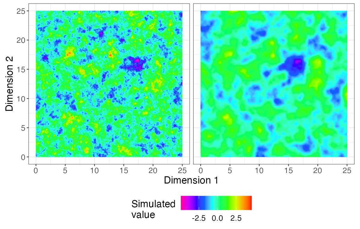
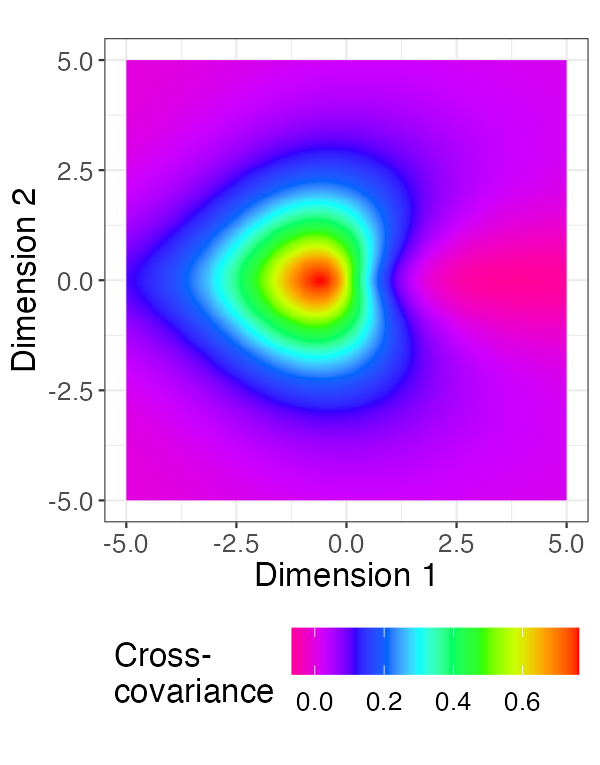
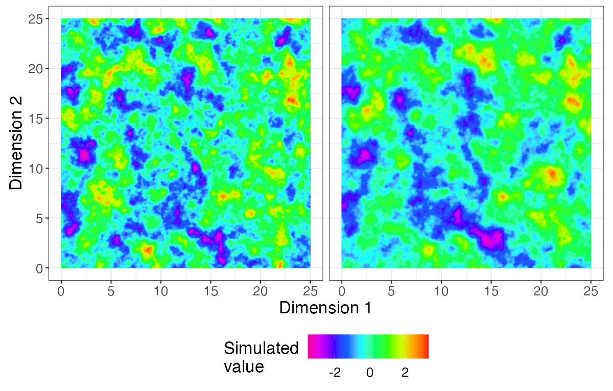
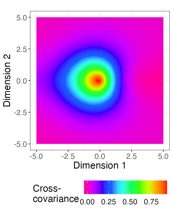
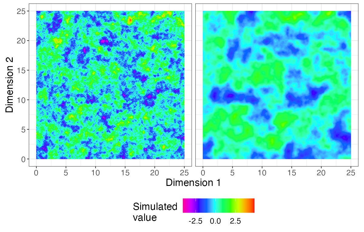
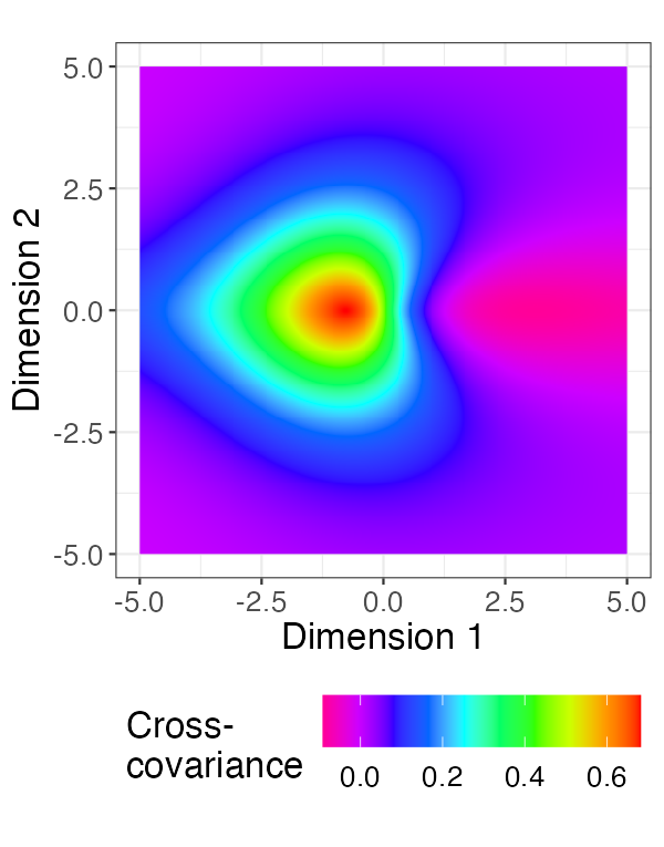
Figure 6: Simulated realizations of process $j$ (Left) and Process $k$ (Middle) over a grid from $0$ to $25$; (Right) their cross-covariance function. For each process, we take $\boldsymbol{\mu}(d\boldsymbol{\theta})=\boldsymbol{\Sigma}d\boldsymbol{\theta}$, $\sigma_{jj}=\sigma_{kk}=1$, $\sigma_{jk}=0.85$, $\varphi(\boldsymbol{\theta})=\textrm{sign}(\theta_{1})$ where $\theta_{1}$ is the first entry of $\boldsymbol{\theta}$. (Top) $a_{j}=a_{k}=1$, $\nu_{j}=0.5$, $\nu_{k}=1.5$. (Middle) $a_{j}=1.2$, $a_{k}=0.8$, and $\nu_{j}=\nu_{k}=1$. (Bottom) $a_{j}=1.1$, $a_{k}=0.9$, and $\nu_{j}=0.5$, and $\nu_{k}=1.5$.

4.3 Cross-covariances with imaginary or varying directional measure

Next, we explore the flexibility that $\boldsymbol{\mu}(d\boldsymbol{\theta})$ provides and the resulting cross-covariances. We first outline one particular area where the result is directly comparable to the $d=1$ case. Suppose that $\mu_{jk}(d\boldsymbol{\theta})=\textrm{sign}(\theta_{1})\mathbbm{i}d\boldsymbol{\theta}$, where $\theta_{1}$ is the first entry of the vector $\boldsymbol{\theta}$. We choose this axis arbitrarily, and such a formulation can be extended to the conditions of $\langle\boldsymbol{\theta}^{*},\boldsymbol{\theta}\rangle>0$ and $<0$, and so forth for some fixed vector $\boldsymbol{\theta}^{*}$. Finally, let $\nu=\nu_{j}=\nu_{k}>0$, $\nu\notin m/2$ for $m\in\mathbb{N}$, and $a=a_{j}=a_{k}>0$, so that we are left with a cross-covariance of

$$C_{jk}(\boldsymbol{h}) =c_{j}c_{k}\int_{0}^{\infty}\int_{\mathcal{S}^{d-1}}e^{\mathbbm{i}\langle\boldsymbol{h},r\boldsymbol{\theta}\rangle}\left(a^{2}+r^{2}\right)^{-\nu-\frac{d}{2}}$$

$$~{}~{}~{}~{}~{}~{}~{}~{}\times\mathbbm{i}\textrm{sign}(\theta_{1})r^{d-1}d\boldsymbol{\theta}dr.$$

First, take $\boldsymbol{h}$ to have first entry $0$ so that we may write $\boldsymbol{h}\in\textrm{span}\{\boldsymbol{e}_{2},\boldsymbol{e}_{3},\dots,\boldsymbol{e}_{d}\}$ where $\boldsymbol{e}_{q}$ is the $q$-th standard basis function. Then, as the integrand is an odd function of $\theta_{1}$, we have

$$\int_{\mathcal{S}^{d-1}}e^{\mathbbm{i}\langle\boldsymbol{h},r\boldsymbol{\theta}\rangle}\textrm{sign}(\theta_{1})d\boldsymbol{\theta}=0.$$

This implies an axis of reflection across $\boldsymbol{e}_{1}$ where $C_{jk}(\boldsymbol{h})=0$ for any $\boldsymbol{h}$ with first entry $0$. Alternately, when $\boldsymbol{h}$ points in the orthogonal direction, that is, $\boldsymbol{h}=b\boldsymbol{e}_{1}$ for $b\in\mathbb{R}$, we outline in Section B how then

$$C_{jk}(b\boldsymbol{e}_{1})\propto\textrm{sign}(b)\left|ba_{j}^{-1}\right|^{\nu_{j}}\left(L_{-\nu_{j}}(a_{j}|b|)-I_{\nu_{j}}(a_{j}|b|)\right).$$

The cross-covariance in this direction has the same form as in the $d=1$ case of imaginary entries, a natural generalization to the $d>1$ case. We also confirm this result numerically in the code accompanying this paper. An example of this cross-covariance is plotted in the top panel of Figure 7. To develop this closed form to general $\boldsymbol{h}$, we have explored incomplete cylindrical functions as described in Agrest and Maksimov, (1971), yet this does not appear to properly generalize the results here.

The above is just one example of the flexibility that the measure $\boldsymbol{\mu}$ provides, and there is a broad array of potential symmetries in the domain of the process. Didier et al., (2018) provide more insight about the possibilities, characterizing all domain and range symmetries in the case $p=d=2$ for operator fractional Brownian fields. As one example, we plot another cross-covariance with more complicated $\boldsymbol{\mu}(d\boldsymbol{\theta})$ in the bottom panel of Figure 7.

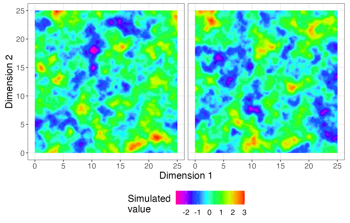
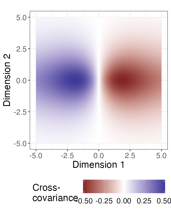
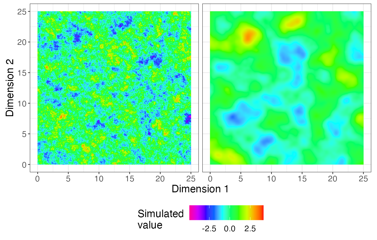
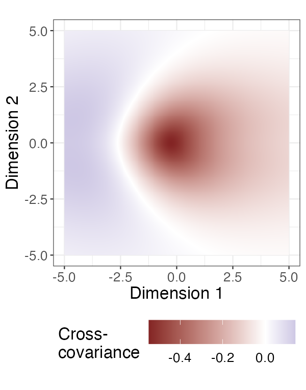
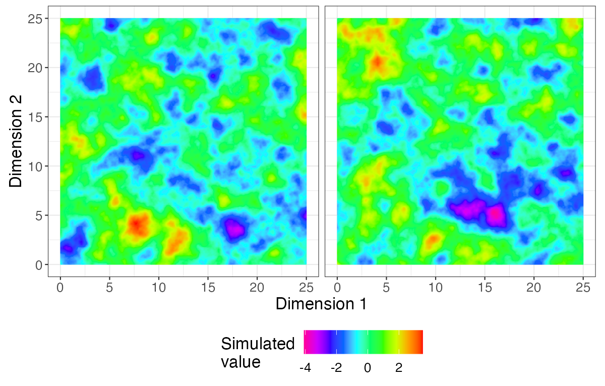
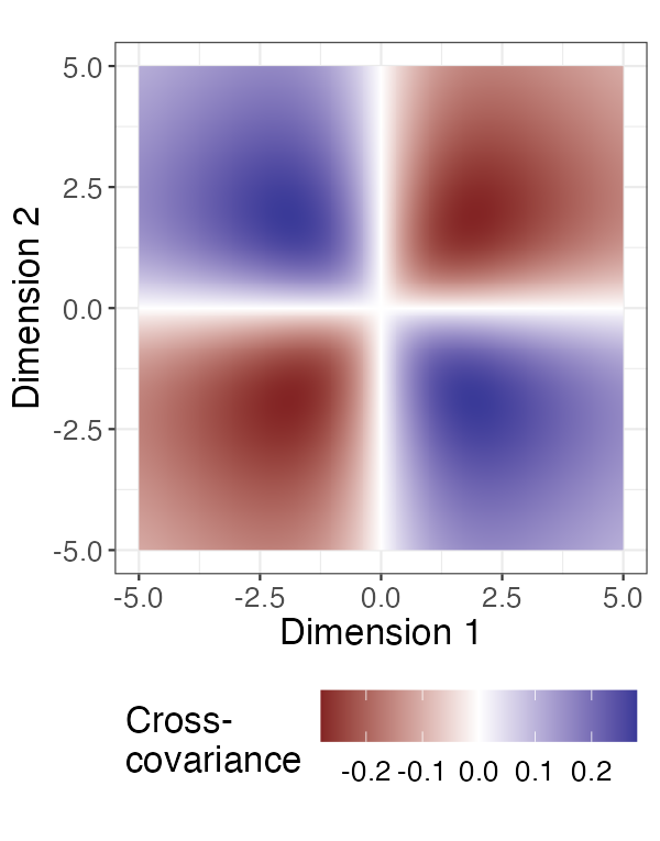
Figure 7: Simulated realizations of process $j$ (Left) and Process $k$ (Middle) over a grid from $0$ to $25$; (Right) their cross-covariance function. For each process, we take $a_{j}=a_{k}=1$, $\varphi(\boldsymbol{\theta})=\textrm{sign}(\theta_{1})$, $\mu_{jj}(d\boldsymbol{\theta})=\mu_{kk}(d\boldsymbol{\theta})=d\boldsymbol{\theta}$, and normalization A. (Top) With $\nu_{j}=\nu_{k}=1.5$, $\mu_{jk}(d\boldsymbol{\theta})=0.97\mathbbm{i}\textrm{sign}(\theta_{1})d\boldsymbol{\theta}$. (Middle) With $\nu_{j}=0.4$, $\nu_{k}=2.5$, and $\mu_{jk}(d\boldsymbol{\theta})=0.97\mathbbm{i}\textrm{sign}(\theta_{1})d\boldsymbol{\theta}$. (Bottom) With $\nu_{j}=\nu_{k}=1.5$ and $\mu_{jk}(d\boldsymbol{\theta})=0.97\left(\textrm{sign}(\theta_{1})\times\textrm{sign}(\theta_{2})\right)d\boldsymbol{\theta}$.

By considering general complex forms for $\boldsymbol{\mu}(d\boldsymbol{\theta})$, we introduce a wide class of spatial cross-covariance functions for $d\geq 2$. They are a natural extension of the Matérn covariance as well as a natural extension of the new multivariate Matérn models when $d=1$. There is a wide amount of model flexibility, especially with respect to the input domain. For practitioners, it may be helpful to understand which type of asymmetries are likely and impose relevant restrictions on the functions $\boldsymbol{\mu}(d\boldsymbol{\theta})$ and $\varphi(\boldsymbol{\theta})$. These computations for such a flexible model are ameliorated by computational approaches for multivariate Fourier transforms on Euclidean or polar grids; for example, see Averbuch et al., (2006).

5 Data analysis

We next demonstrate the estimation of these new multivariate Matérn models in the context of spatial data. In particular, most previous work has considered air pressure and temperature data in the Pacific Northwest of North America (see Gneiting et al.,, 2010; Apanasovich et al.,, 2012; Bolin and Wallin,, 2019; Cressie and Zammit-Mangion,, 2016; Hu et al.,, 2013). We also analyze ocean temperature data collected by Argo floats, which is studied in Bolin and Wallin, (2019).

For both datasets, we use $\boldsymbol{s}\in\mathbb{R}^{2}$ and have $p=2$. To evaluate covariances and cross-covariances, we use a 2-dimensional inverse Fourier transform implemented through Frigo, (1999) on a regular and fine grid. Covariance values are then interpolated onto the actual distances between sites. For model estimation, we employ maximum likelihood estimation under a Gaussian assumption. Let $\boldsymbol{X}_{obs,1}=[X_{1}(\boldsymbol{s}_{i})]_{i=1}^{n_{1}}\in\mathbb{R}^{n_{1}}$ and $\boldsymbol{X}_{obs,2}=[X_{2}(\boldsymbol{s}_{i})]_{i=1}^{n_{2}}\in\mathbb{R}^{n_{2}}$ be vectors of the two variables, respectively. We suppose that

$$\begin{pmatrix}\boldsymbol{X}_{obs,1}\\ \boldsymbol{X}_{obs,2}\end{pmatrix} \sim\mathcal{N}_{n_{1}+n_{2}}\Bigg{(}\begin{pmatrix}\mu_{1}\mathbbm{1}_{n_{1}}\\ \mu_{2}\mathbbm{1}_{n_{2}}\end{pmatrix},$$

$$~{}~{}~{}~{}~{}~{}~{}~{}~{}\boldsymbol{\Gamma}:=\begin{pmatrix}\boldsymbol{\Sigma}_{11}+\gamma^{2}_{1}\boldsymbol{I}_{n_{1}}&\boldsymbol{\Sigma}_{12}\\ \boldsymbol{\Sigma}_{12}^{\top}&\boldsymbol{\Sigma}_{22}+\gamma^{2}_{2}\boldsymbol{I}_{n_{2}}\end{pmatrix}\Bigg{)}.$$

Adding the nugget effect terms of $\gamma^{2}_{1}$ and $\gamma^{2}_{2}$ is commonly done in spatial statistics applications including previous ones with this data (for example, Gneiting et al.,, 2010; Apanasovich et al.,, 2012). In addition, we focus on estimation of the covariance structure and subtract the empirical mean from each variable of the observations. We then estimate the parameters governing $\boldsymbol{\Sigma}_{11}$, $\boldsymbol{\Sigma}_{12}$, $\boldsymbol{\Sigma}_{22}$ as well as $\gamma^{2}_{1}$ and $\gamma^{2}_{2}$ using maximum likelihood estimation. Since closed-form representation of the maximum likelihood estimates are not generally available, we numerically optimize the likelihood using the L-BFGS-B routine in R (Byrd et al.,, 1995).

We now define the models we compare:

1. Independent Matérn, where the processes are estimated independently, so that $\boldsymbol{\Sigma}_{12}=\boldsymbol{0}$, and $\boldsymbol{\Sigma}_{11}$ and $\boldsymbol{\Sigma}_{22}$ are defined by univariate Matérn covariances.

2. A “single covariance function” model, with

   $$\boldsymbol{\Gamma} =\begin{pmatrix}\sigma_{11}&\sigma_{12}\\ \sigma_{12}&\sigma_{22}\end{pmatrix}\otimes\boldsymbol{\Sigma}_{single}+\begin{pmatrix}\gamma^{2}_{1}\boldsymbol{I}_{n}&\boldsymbol{0}_{n\times n}\\ \boldsymbol{0}_{n\times n}&\gamma^{2}_{2}\boldsymbol{I}_{n}\end{pmatrix}.$$

   Here, $\boldsymbol{\Sigma}_{single}$ is a correlation matrix defined with a Matérn covariance at the observed points, and $\otimes$ is the standard Kronecker product, so that each covariance and cross-covariance has the same shape.

3. The multivariate Matérn of Gneiting et al., (2010) using the parameters $\nu_{1}$, $\nu_{2}$, $\nu_{12}$, $a_{1}$, $a_{2}$, $a_{12}$, $\sigma_{11}$, $\sigma_{12}$, $\sigma_{22}$, $\gamma^{2}_{1}$, and $\gamma^{2}_{2}$.

4. A spectral multivariate Matérn as presented in Section 4, with real directional measure and $\varphi(\boldsymbol{\theta})=\textrm{sign}(\theta_{1})$ fixed and not estimated. The parameters are $\nu_{1}$, $\nu_{2}$, $a_{1}$, $a_{2}$, $\sigma_{11}$, $\sigma_{12}$, $\sigma_{22}$, $\gamma^{2}_{1}$, and $\gamma^{2}_{2}$.

5. A spectral multivariate Matérn as presented in Section 4, with real directional measure and $\varphi(\boldsymbol{\theta})=\textrm{sign}\left(\boldsymbol{\theta}^{\top}\boldsymbol{\theta}^{*}\right)$ for a fixed $\boldsymbol{\theta}^{*}$ that we estimate.

6. A spectral multivariate Matérn as presented in Section 4, with complex directional measure $\mu_{12}(d\boldsymbol{\theta})=\Re(\sigma_{12})+\Im(\sigma_{12})\mathbbm{i}\textrm{sign}\left(\boldsymbol{\theta}^{\top}\boldsymbol{\theta}^{*}_{1}\right)d\boldsymbol{\theta}$ and the function $\varphi(\boldsymbol{\theta})=\textrm{sign}\left(\boldsymbol{\theta}^{\top}\boldsymbol{\theta}^{*}_{2}\right)$ for two different estimated parameters $\boldsymbol{\theta}^{*}_{1}$ and $\boldsymbol{\theta}^{*}_{2}$.

5.1 Pacific Northwest weather data

The data consists of $n=157$ of bivariate measurements indexed in $\mathbb{R}^{2}$. After converting relevant distances to kilometers, the maximum distance between two locations is $1{,}561.6$ kilometers. Thus, for the discrete Fourier transform, we use $2^{10}=1{,}024$ points for each dimension evenly-spaced between $-2{,}500$ and $2{,}500$ kilometers.

We now present the results comparing the models as applied to the data. For equal comparison, we use the Fourier-transform-based optimization of the likelihood for each model. In Table 2, we provide details of the estimated maximized log-likelihoods of the models. First, in comparing the log-likelihoods, the multivariate Matérn of Gneiting et al., (2010) and the models introduced here have a higher maximum likelihoods and mostly lower Akaike information criteria (AIC) compared to the independent Matérn and single covariance function models. This suggests moderately better fits of SMM-0 and SMM-R in fitting the cross-covariance of pressure and temperature. In comparing the three SMM models, we see that increasing complexity of the model results in a larger maximized log-likelihood yet also higher AIC values. This suggests that increased complexity in the SMM-C model may not be suitable for this dataset.

We also present the optimized parameters in Tables 3 and 4 for temperature (process 1) and pressure (process 2). For the most part, the estimated parameters and log-likelihoods are also consistent with previous analyses of the data (Gneiting et al.,, 2010); differences (for example, an estimated $\nu_{1}=1.50$ is reported in Gneiting et al.,, 2010) are likely due to the Fourier transform estimation scheme. The estimated parameters of SMM models are mostly consistent with each other and the multivariate Matérn of Gneiting et al., (2010). The SMM models introduced in this paper have a stronger correlation parameter compared to the other models, which may be expected since the cross-correlation functions often take maximum absolute value substantially less than $1$ (see Figure 6). The estimate of $\Im(\sigma_{12})$ suggests marginal evidence of covariance irreversibility for this data.

Model	Log-likelihood	$\#$ Parameters	AIC
IM	$-1272.304$	8	$2560.608$
SCF	$-1266.664$	7	$2547.328$
MMG	$-1261.418$	11	$2544.836$
SMM-0	$-1261.336$	9	$2540.672$
SMM-R	$-1260.610$	10	$2541.220$
SMM-C	$-1260.537$	12	$2545.074$

Table 2: Multivariate Matérn maximum likelihoods, number of parameters, and Akaike information criterion (AIC) values.

Model	$\nu_{1}$	$\nu_{2}$	$\nu_{12}$	$a_{1}$	$a_{2}$	$a_{12}$
IM	$7.00$	$0.56$	-	$3.3\times 10^{-2}$	$1.0\times 10^{-2}$	-
SCF	$0.50$	-	-	$6.1\times 10^{-3}$	-	-
MMG	$4.27$	$0.59$	$3.23$	$2.4\times 10^{-2}$	$1.1\times 10^{-2}$	$0.024$
SMM-0	$1.13$	$0.55$	-	$8.7\times 10^{-3}$	$9.6\times 10^{-3}$	-
SMM-R	$1.14$	$0.56$	-	$8.6\times 10^{-3}$	$9.9\times 10^{-3}$	-
SMM-C	$1.16$	$0.56$	-	$8.7\times 10^{-3}$	$9.9\times 10^{-3}$	-

Table 3: Multivariate Matérn estimated smoothness and range parameters for the Northwest temperature and pressure data. A dash indicates that the given parameter does not exist under that model.

Model	$\sqrt{\sigma_{11}}$	$\sqrt{\sigma_{22}}$	$\frac{\Re(\sigma_{12})}{\sqrt{\sigma_{11}\sigma_{22}}}$	$\frac{\Im(\sigma_{12})}{\sqrt{\sigma_{11}\sigma_{22}}}$	$\gamma_{1}$	$\gamma_{2}$
IM	$224.93$	$2.63$	-	-	$71.37$	$1.27\times 10^{-2}$
SCF	$198.57$	$3.02$	$-0.389$	-	$48.03$	$1.70\times 10^{-3}$
MMG	$225.69$	$2.63$	$-0.554$	-	$72.03$	$2.24\times 10^{-2}$
SMM-0	$226.37$	$2.66$	$-0.661$	-	$68.16$	$3.64\times 10^{-3}$
SMM-R	$226.21$	$2.65$	$-0.683$	-	$69.19$	$3.64\times 10^{-3}$
SMM-C	$227.41$	$2.65$	$-0.685$	$-0.039$	$69.38$	$3.64\times 10^{-3}$

Table 4: Estimated variance parameters for the Northwest temperature and pressure data. A dash indicates that the given parameter does not exist under that model.

In Figure 8, we plot the estimated cross-covariance functions for each of the models. We see that the single covariance function and the multivariate Matérn of Gneiting et al., (2010) are isotropic and covariance-reversible, while each of the SMM have more flexible form. Furthermore, the estimated cross-covariance between the processes is substantially larger for lags of approximately 50-300 kilometers for the SMM models compared to the other models.

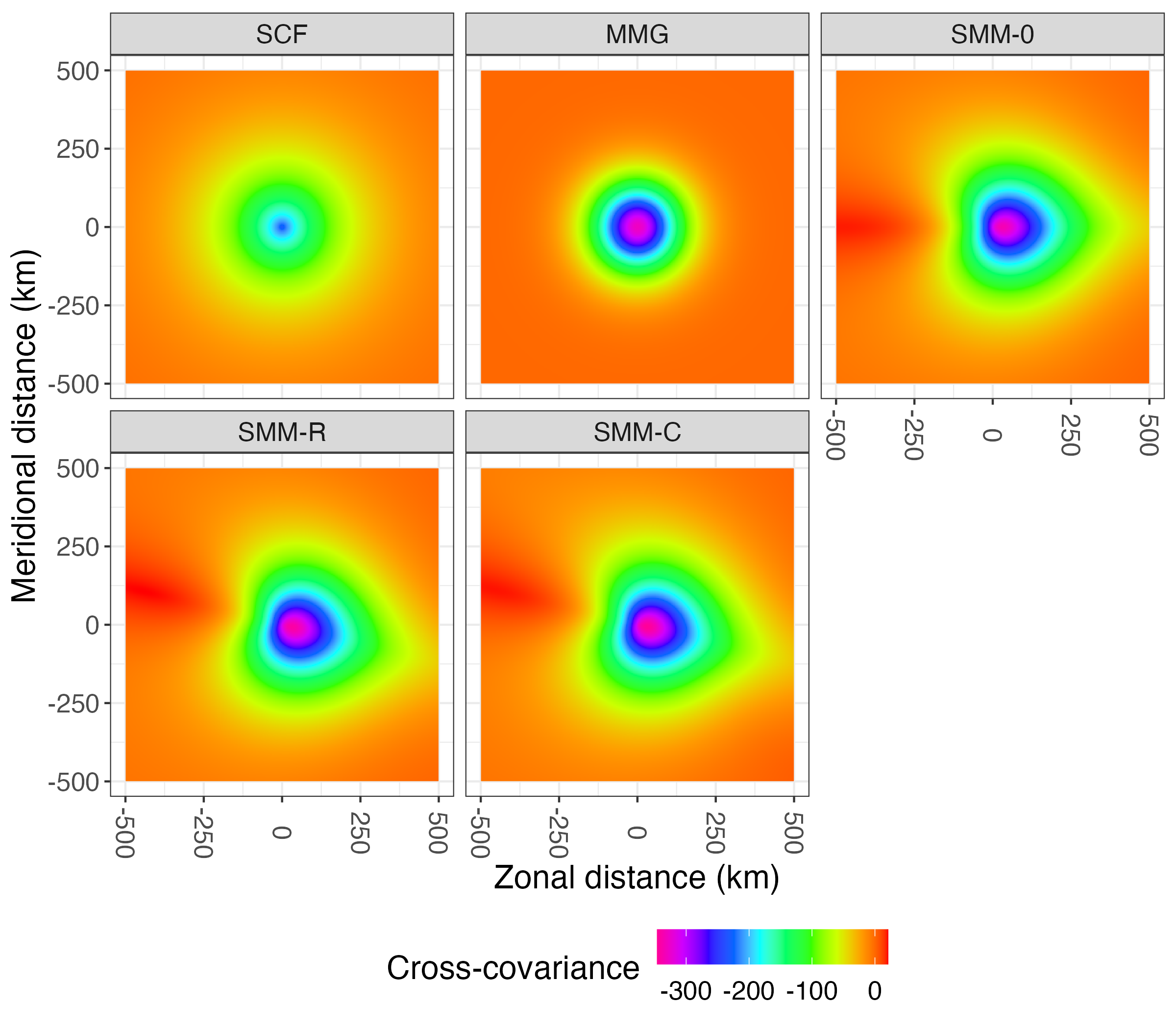
Figure 8: Estimated cross-covariance functions on the Pacific Northwest pressure and temperature data. Zonal distance refers to distance in the east-west (longitude) direction, and meridional distance refers to distance in the north-south (latitude) direction.

To compare predictive performance, we evaluate the estimated models in their prediction using cross-validation. Predictions are formed using standard expressions for the conditional expectation. We consider 5-fold and $n$-fold cross validation, where a proportion of $1/5$ or $1/n$ of data points are left out of the dataset for one variable, and a prediction is formed using the rest of the data of that variable as well as all data of the other variable. We repeat this for both variables comparing root-mean-squared-error averaged across the folds. For comparison, we also predict using only the data of the target variable, as well as only data using the other variables. Results are presented in Table 5. Using both variables improves using only one of the variables at a time, and prediction errors are expectedly lower for $n$-fold compared to 5-fold cross-validation. In general, there are not large gaps in prediction performance between the multivariate Matérn of Gneiting et al., (2010) and the SMM models, and for the most part the SMM provide slightly improved point prediction performance. Overall, we find that the SMM models introduced in this paper can fit as well or better than the multivariate Matérn of Gneiting et al., (2010) on this standard dataset.

Model	5f-both	5f-univariate	$n$f-both	$n$f-univariate	other
Prediction of zero	194.2494	194.2494	194.2494	194.2494	194.2494
SCF	125.2853	132.5836	172.9075	123.4839	172.9075
MMG	126.6086	134.0422	117.2287	119.0559	176.6753
SMM-0	122.7652	132.8396	116.7819	121.1790	164.7258
SMM-R	123.1258	132.8966	116.5281	121.2294	164.6401
SMM-C	122.8856	132.9320	116.4606	121.2207	165.7362

Model	5f-both	5f-univariate	$n$f-both	$n$f-univariate	other
Prediction of zero	2.709560	2.709560	2.709560	2.709560	2.709560
SCF	1.672005	1.693611	1.582059	1.620309	2.391110
MMG	1.631760	1.690111	1.545588	1.624545	2.390009
SMM-0	1.631041	1.689291	1.560799	1.624241	2.228422
SMM-R	1.611251	1.689463	1.540141	1.624176	2.225494
SMM-C	1.612860	1.689452	1.542120	1.624203	2.229628

Table 5: Cross-validation root-mean-squared error (RMSE) results compared for 5-fold (5f) and $n$-fold ($n$f) cross-validation. Columns with “both” use both variables to predict at the left-out points, “univariate” uses just the target variable, and “other” uses just the other variable (and thus does not depend on the number of folds). These values are compared with the null prediction of $0$ as a baseline. The lowest values in each column are bold. (Top) For pressure. (Bottom) For temperature.

5.2 Argo temperature data

We now turn to the Argo data which profiles temperature and salinity measurements in the upper $2{,}000$ meters of the ocean (Argo,, 2020). Here, we focus on temperature measurements at the depths of $300$ meters and $1{,}500$ meters located south of New Zealand in the year 2015 and fit a bivariate model to them. This data was also used in Bolin and Wallin, (2019), and an extensive analysis of Argo data using univariate spatial models is presented in Kuusela and Stein, (2018). We present parameter estimates and log-likelihoods in Appendix C. The estimated cross-covariances are plotted in Figure 9. The multivariate Matérn with complex directional measure shows a substantially different shape of the cross-covariance compared to the other models, and there is a substantially strong imaginary component to the cross-covariance. While the estimated real correlation parameter for the SMM-R model is $0.678$, the estimated real and imaginary correlation parameter for the SMM-C model are $0.638$ and $0.275$, respectively. This demonstrates that the imaginary component of the model is substantial, and its introduction does not considerably detract from the estimated strength of the real component of the model.

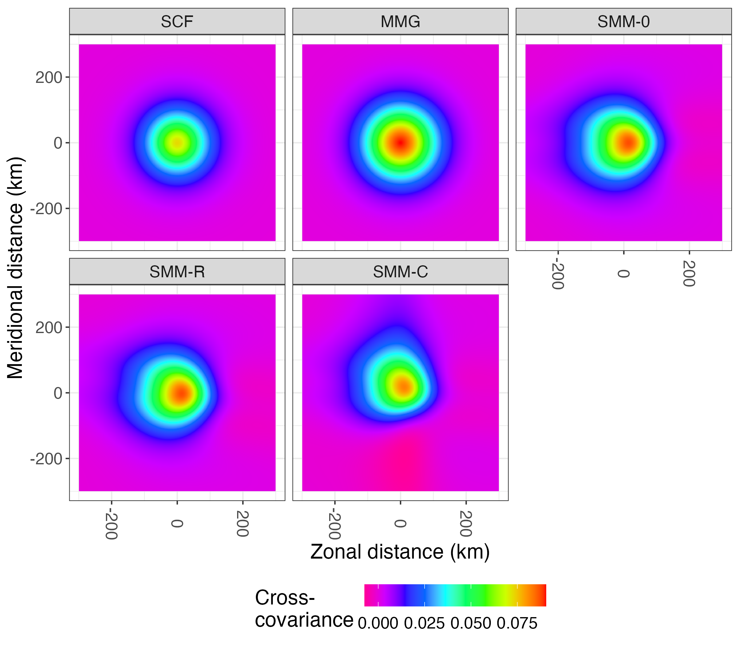
Figure 9: Estimated cross-covariance functions on the Argo temperature data.

6 Discussion and extensions

In this work, we introduce a new class of multivariate Matérn models motivated by the spectral representation of the Matérn covariance. This class of models provides more flexible forms of the cross-covariance structure compared to the multivariate Matérn of Gneiting et al., (2010) and its more recent extensions. In particular, asymmetry in the cross-covariance can be modeled straightforwardly. Furthermore, compared to that of the multivariate Matérn of Gneiting et al., (2010), there are fewer parameters for $d=1$ and validity of the cross-covariance is given without complicated restrictions on the parameters. We also provide clarity on how previous work on multivariate Matérn models fit into the framework developed here. Under particular parameters in the time series setting of $d=1$, closed-form expressions for the cross-covariance are given.

In the spatial case of $d\geq 2$, flexible representations of the cross-covariance with respect to the domain are available. A potentially fruitful area of further research would be to investigate the extent of the existence of closed-form spatial covariances. On the other hand, the flexibility of such models suggests that closed-form cross-covariances may be elusive, and we have explored possible approaches (for example, in Agrest and Maksimov,, 1971; Babister,, 1967) to no avail. To mitigate this challenge, we demonstrate that spatial processes with these cross-covariances can be easily simulated using existing approaches for multivariate random fields, and the cross-covariance functions can be evaluated through their spectral density.

There are some research avenues that could strengthen our understanding of the models introduced here. First, it is unclear which parameters of the cross-covariance are identifiable under fixed-domain asymptotics. In the univariate setting, the parameters $a_{j}$ and $\sigma_{jj}$ are not individually identifiable (Zhang,, 2004). Thus, it is unclear if the real and imaginary parts of $\boldsymbol{\mu}(d\boldsymbol{\theta})$ would be identifiable; if so, a statistical test for the null hypothesis $\boldsymbol{\mu}(d\boldsymbol{\theta})\in\mathbb{R}^{p\times p}$ could be developed. Also, the parameter $\varphi(d\boldsymbol{\theta})$ is relatively mysterious, especially in the case $d\geq 2$; it may be possible that one can choose a separate $\varphi(d\boldsymbol{\theta})$ for each cross-covariance when $p>2$. Future work could also introduce computational methodology to use the model presented here for large-scale data analysis; such work for previous multivariate Matérn models includes Fahmy and Guinness, (2022).

We conclude with a few potential extensions of this work that may be of interest to the spatial statistics community.

6.1 SPDE approach

The new multivariate Matérn models should relate to the characterizations of the Matérn model and fractional Brownian motion through stochastic partial differential equations (SPDEs) (Lindgren et al.,, 2011; Tafti and Unser,, 2010). Hu et al., (2013) adapt the SPDE approach to the multivariate Matérn of Gneiting et al., (2010) by considering the system

$$\begin{pmatrix}\mathcal{L}(a_{1},\nu_{1})&\mathcal{L}(a_{12},\nu_{12})\\ 0&\mathcal{L}(a_{2},\nu_{2})\end{pmatrix}\begin{pmatrix}Y_{1}(s)\\ Y_{2}(s)\end{pmatrix}=\begin{pmatrix}\mathcal{W}_{1}\\ \mathcal{W}_{2}\end{pmatrix},$$ (6.1)

where $\mathcal{W}_{j}$ are independent (and, in most cases, Gaussian) white noise processes, $\mathcal{L}(a,\nu)=(a^{2}\boldsymbol{I}-\Delta)^{(\nu+\frac{1}{2})/2}$, and $\Delta$ is the Laplacian operator. Bolin and Wallin, (2019) consider an alternative approach that also uses the SPDE formulation as an inspiration. Our approach suggests a new strategy; for the example of $d=1$, one can consider differential operators generated by convolutions of $G^{a,-\mu}_{+}$ and $G^{a,-\mu}_{-}$, which are in turn characterized using fractional calculus through the Fourier transform $\mathcal{F}$ with

$$\mathcal{F}\left[G_{\pm}^{a,\mu}f(y)\right]=(a\mp\mathbbm{i}x)^{-\mu}\mathcal{F}\left[f(x)\right]$$

in a similar manner to Section 18.4 of Samko et al., (1993). Through their Fourier transforms, one sees that $G_{-}^{a,-\mu}*G_{+}^{a,-\mu}=(a^{2}\boldsymbol{I}-\Delta)^{\mu}$ where $*$ is the convolution. Therefore, each operator associated with the Matérn processes (for example, in Equation 6.1) can be formed from convolutions of $G_{\pm}^{a,\mu}$ operators. The operators $G_{\pm}^{a,-\mu}$ relate to the differential operators $(a\boldsymbol{I}\mp\nabla)^{\mu}$ where $\nabla$ is the derivative operator, as outlined in Section 18.4 of Samko et al., (1993). See Appendix B of Lindgren et al., (2011) and Sections 27 and 18.4 of Samko et al., (1993) for further details. However, more care must be taken to extend such an approach to $d=2,3,\dots$ and a complex-valued directional measure.

6.2 Functional Matérn models

Extending this model from multivariate to functional data would be of theoretical and practical interest for a variety of spatial functional data analysis applications (see, for example, Martínez-Hernández and Genton,, 2020). Shen et al., (2022) develop a framework for covariance models in a general separable Hilbert space $\mathbb{V}$, which is a setting broader than the $\mathbb{R}^{p}$-valued processes here. In particular, they extend the results of Cramér, (1942), so that a process $X(\boldsymbol{s})$ taking values in $\mathbb{V}$ can be written

$$X(\boldsymbol{s}) =\int_{\mathbb{R}^{d}}e^{\mathbbm{i}\langle\boldsymbol{s},\boldsymbol{x}\rangle}\eta(d\boldsymbol{x}),$$

where $\eta(d\boldsymbol{x})$ is an appropriately-defined $\mathbb{V}$-valued random measure. Similarly to Proposition 5.6 of Shen et al., (2022), one might consider

$$X(\boldsymbol{s}) =\int_{0}^{\infty}\int_{\mathcal{S}^{d-1}}e^{\mathbbm{i}\langle\boldsymbol{s},r\boldsymbol{\theta}\rangle}(a+\varphi(\boldsymbol{\theta})\mathbbm{i}r)^{-\nu-\frac{d}{2}}\boldsymbol{B}_{\boldsymbol{\mu}}(dr,d\boldsymbol{\theta}),$$

where $\mathbb{E}\left[\boldsymbol{B}_{\boldsymbol{\mu}}(dr,d\boldsymbol{\theta})\otimes\boldsymbol{B}_{\boldsymbol{\mu}}(dr,d\boldsymbol{\theta})\right]=r^{d-1}dr\boldsymbol{\mu}(d\boldsymbol{\theta})$, $\otimes$ is the outer product on $\mathbb{V}$, and $\boldsymbol{\mu}(d\boldsymbol{\theta})$ is now a positive-definite and trace-class operator on $\mathbb{V}$. Extensions to where $\nu$ and $a$ are also operators would introduce flexible covariances for the spatial functional-data setting.

6.3 Alternate factorization of spectral density

As suggested by (1.6), one may also study the covariance given by

$$C_{jk}(\boldsymbol{h}) =c_{j}c_{k}\int_{0}^{\infty}\int_{\mathcal{S}^{d-1}}e^{\mathbbm{i}\langle\boldsymbol{h},r\boldsymbol{\theta}\rangle}\left(a_{j}^{2}+r^{2}\right)^{-\frac{\nu_{j}}{2}-\frac{d}{4}}$$

$$~{}~{}~{}~{}\times\mu_{jk}(d\boldsymbol{\theta})\left(a_{k}^{2}+r^{2}\right)^{-\frac{\nu_{k}}{2}-\frac{d}{4}}dr.$$

This model was studied for real-valued and constant $\boldsymbol{\mu}(d\boldsymbol{\theta})$ in Bolin and Wallin, (2019). The form suggests that, when $\mu_{jk}(d\boldsymbol{\theta})\propto d\boldsymbol{\theta}$, the cross-covariance is isotropic for any appropriate $a_{j}$, $a_{k}$, $\nu_{j}$, and $\nu_{k}$; alternately, when $\boldsymbol{\mu}(d\boldsymbol{\theta})\propto\mathbbm{i}\textrm{sign}(\boldsymbol{\theta}^{\top}\boldsymbol{\theta}^{*})d\boldsymbol{\theta}$ for a fixed $\boldsymbol{\theta}^{*}$, the cross-covariance would be reflected across the direction perpendicular to $\boldsymbol{\theta}^{*}$ for any values of the inverse range and smoothness parameters. This cross-covariance also allows one to avoid the introduction of $\varphi(\boldsymbol{\theta})$ when $d\geq 2$. However, closed-form expressions of this covariance seem to be more elusive. One exception is the case of $d=1$, $\nu_{j}=\nu_{k}=3/2$, and real directional measure: we see that

$$\begin{split}&C_{jk}(h)=2c_{j}c_{k}\Re(\sigma_{jk})\int_{0}^{\infty}\cos(hx)\\ &~{}~{}~{}~{}~{}\times\left(a_{j}^{2}+x^{2}\right)^{-\frac{\nu_{j}}{2}-\frac{1}{4}}\left(a_{k}^{2}+x^{2}\right)^{-\frac{\nu_{k}}{2}-\frac{1}{4}}dx,\end{split}$$ (6.2)

and by 3.728 (1) of Gradshteyn et al., (2015),

$$C_{jk}(h) =c_{j}c_{k}\Re(\sigma_{jk})\frac{\pi}{a_{j}a_{k}}\frac{a_{j}e^{-a_{k}|h|}-a_{k}e^{-a_{j}|h|}}{a_{j}^{2}-a_{k}^{2}}$$

for $a_{j}\neq a_{k}$ (the case $a_{j}=a_{k}$ is Matérn). We plot examples of these cross-covariances in Figure 10.

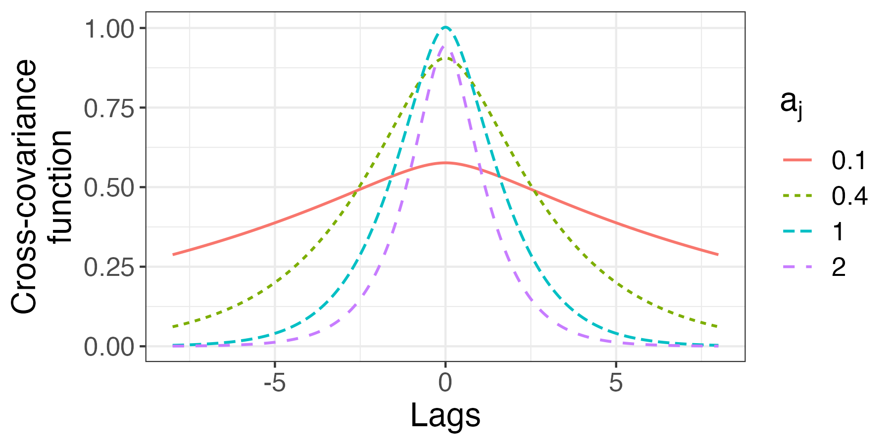
Figure 10: Multivariate Matérn cross-covariances of type (6.2) for $\Re(\sigma_{jk})=1$, $a_{k}=1$, $\nu_{j}=\nu_{k}=3/2$ and $a_{j}$ varying.

6.4 Applications to other covariance functions

Factoring the spectral density and using a complex-valued variance parameterization, as done in this paper, should be considered more generally as a way to flexibly extend covariance functions to the multivariate case. For example, consider the squared-exponential covariance function for $d=1$ which has covariance function $C(h)=\textrm{exp}(-ah^{2})$ and spectral density function $f(x)=(\pi a)^{-\frac{1}{2}}\textrm{exp}(-x^{2}/(4a))/2$ (see Section 2.7 of Stein,, 1999). Considering a cross-spectral density of

$$f_{jk}(x) =\frac{1}{2\sqrt{\pi}a_{j}^{\frac{1}{4}}a_{k}^{\frac{1}{4}}}\textrm{exp}\left(-\frac{x^{2}}{8a_{j}}-\frac{x^{2}}{8a_{k}}\right)$$

$$~{}~{}~{}~{}~{}~{}~{}\times(\Re(\sigma_{jk})+\mathbbm{i}\Im(\sigma_{jk})\textrm{sign}(x))$$

leads to a cross-covariance function of

$$C_{jk}(h) =\frac{(a_{j}a_{k})^{\frac{1}{4}}}{\sqrt{a_{+}}}\Bigg{[}\Re(\sigma_{jk})\textrm{exp}\left(-\frac{a_{j}a_{k}}{a_{+}}h^{2}\right)$$

$$~{}~{}~{}~{}~{}~{}~{}~{}~{}~{}~{}~{}~{}~{}~{}~{}~{}~{}~{}~{}~{}-\Im(\sigma_{jk})\frac{2}{\sqrt{\pi}}\tilde{F}\left(\sqrt{\frac{a_{j}a_{k}}{a_{+}}}h\right)\Bigg{]},$$

where $a_{+}=(a_{j}+a_{k})/2$ and $\tilde{F}(z)$ is Dawson’s integral, an odd function of $z$. The cross-covariance reduces to the squared-exponential covariance function when $a_{j}=a_{k}$ and $\Im(\sigma_{jk})=0$, and properties of the cross-covariances including asymptotic expansions follow from those of the exponential function and Dawson’s integral. One could conceivably extend this formulation to the more general powered-exponential class or other classes of models like the generalized Cauchy covariance (cf. Moreva and Schlather,, 2023).

7 Acknowledgements

The Argo data was collected and made freely available by the International Argo Program and the national programs that contribute to it. (https://argo.ucsd.edu, https://www.ocean-ops.org). The Argo Program is part of the Global Ocean Observing System.

Appendix A Hilbert transforms

Proposition A.1.

The Hilbert transform of $-a|h|e^{-a|h|}$ is

$$-a|h|R(h,a,a)+\frac{2ahe^{a|h|}}{\pi}\textrm{Ei}(-a|h|).$$

Proof.

In particular, we look at the Hilbert transform, add and subtract $x$ in the numerator, and break out the integral into multiple terms:

$$\mathcal{H}(|h|e^{-|a|h}) =\frac{1}{\pi}\int_{-\infty}^{\infty}\frac{|s|e^{-a|s|}}{x-s}ds$$

$$=\frac{1}{\pi}\int_{-\infty}^{\infty}\frac{(x-(x-|s|))e^{-a|s|}}{x-s}ds$$

$$=\frac{1}{\pi}x\int_{-\infty}^{\infty}\frac{e^{-a|s|}}{x-s}ds-\frac{1}{\pi}\int_{-\infty}^{\infty}\frac{(x-|s|)e^{-a|s|}}{x-s}ds.$$

Notice that the first term is $x\mathcal{H}(e^{-a|s|})$. Breaking down the remaining integral, we obtain

$$\mathcal{H}(|h|e^{-|a|h}) =x\mathcal{H}(e^{-a|s|})-\frac{1}{\pi}\int_{0}^{\infty}e^{-as}ds$$

$$~{}~{}~{}~{}~{}~{}-\frac{1}{\pi}\int_{-\infty}^{0}\frac{(x+s)e^{-a|s|}}{x-s}ds$$

$$=x\mathcal{H}(e^{-a|x|})-\frac{1}{a\pi}-\frac{1}{\pi}\int_{-\infty}^{0}\frac{(x+s)e^{as}}{x-s}ds.$$

Adding and subtracting $s$, we have

$$\int_{-\infty}^{0}\frac{(x+s)e^{as}}{x-s}ds =\int_{-\infty}^{0}\frac{(x-s+2s)e^{as}}{x-s}ds$$

$$=\int_{-\infty}^{0}e^{as}ds+2\int_{-\infty}^{0}\frac{se^{as}}{x-s}ds$$

$$=-\frac{1}{a}+2\int_{-\infty}^{0}\frac{se^{as}}{x-s}ds.$$

Finally,

$$\int_{-\infty}^{0}\frac{se^{as}}{x-s}ds=xe^{a|x|}\textrm{Ei}(-a|x|)$$

follows from a change in variables and the definition of $\textrm{Ei}(z)$.

Combining work, we see that

$$\mathcal{H}(a|h|e^{-|a|h}) =a|h|\mathcal{H}(e^{-a|h|})+\frac{2xe^{a|h|}}{\pi}\textrm{Ei}(-a|h|).$$

The Hilbert transform $\mathcal{H}(e^{-a|h|})$ was established as $-R(h,a,a)$ in the proof of Theorem 3.11.

∎

Appendix B Representation of spatial cross-covariances for imaginary directional measure

We aim to compute

$$C_{jk}(\boldsymbol{h}) =c_{j}c_{k}\int_{0}^{\infty}\int_{\mathcal{S}^{d-1}}e^{\mathbbm{i}\langle\boldsymbol{h},r\boldsymbol{\theta}\rangle}\left(a^{2}+r^{2}\right)^{-\nu-\frac{d}{2}}$$

$$~{}~{}~{}~{}~{}~{}~{}~{}~{}~{}~{}~{}~{}~{}~{}~{}~{}~{}~{}~{}~{}~{}~{}~{}~{}~{}~{}\mathbbm{i}\textrm{sign}(\theta_{1})r^{d-1}d\boldsymbol{\theta}dr.$$

Focusing on the inner integral in the special case where $\boldsymbol{h}=b\boldsymbol{e}_{1}$, we have

$$\mathbbm{i}\int_{\mathcal{S}^{d-1}}e^{\mathbbm{i}\langle\boldsymbol{h},r\boldsymbol{\theta}\rangle}\textrm{sign}(\theta_{1})d\boldsymbol{\theta}$$

$$=\mathbbm{i}\int_{\mathcal{S}^{d-1},\theta_{1}>0}e^{\mathbbm{i}b\theta_{1}r}d\boldsymbol{\theta}-\mathbbm{i}\int_{\mathcal{S}^{d-1},\theta_{1}<0}e^{\mathbbm{i}b\theta_{1}r}d\boldsymbol{\theta}.$$

Applying $e^{\mathbbm{i}b\boldsymbol{\theta}r}=\cos(b\theta_{1}r)+\mathbbm{i}\sin(b\theta_{1}r)$ and using the even and odd properties of cosine and sine, we obtain

$$\mathbbm{i}\int_{\mathcal{S}^{d-1}}e^{\mathbbm{i}\langle\boldsymbol{h},r\boldsymbol{\theta}\rangle}\textrm{sign}(\theta_{1})d\boldsymbol{\theta} =-2\int_{\mathcal{S}^{d-1},\theta_{1}>0}\sin(b\theta_{1}r)d\boldsymbol{\theta}$$

If we approach this integral similarly to page 154 of Stein and Weiss, (1975) or page 43 of Stein, (1999) by making the change of variables to $\phi$, the angle that $\boldsymbol{\theta}$ makes with $\boldsymbol{e}_{1}$, we have

$$\int_{\mathcal{S}^{d-1},\theta_{1}>0}\sin(\theta_{1}br)d\boldsymbol{\theta} \propto\int_{0}^{\pi/2}\sin(\cos(\phi)br)\sin^{d-2}(\phi)d\phi$$

$$\propto(br)^{-(d-2)/2}H_{(d-2)/2}(br)$$

using a standard integral representation of the Struve function $H_{\nu}(z)$, defined as

$$H_{\nu}(z)=\sum_{m=0}^{\infty}\frac{(-1)^{m}(\frac{1}{2}z)^{2m+\nu+1}}{\Gamma(m+\frac{3}{2})\Gamma(m+\nu+\frac{3}{2})}.$$

See Chapter 11 of DLMF, (2021) or Chapter 12 of Abramowitz and Stegun, (1972) for more information. Then, we can apply 6.814 of Gradshteyn et al., (2015) to the overall integral, resulting in a cross-covariance in this direction proportional to

$$\textrm{sign}(b)\left|ba_{j}^{-1}\right|^{\nu_{j}}\left(L_{-\nu_{j}}(a_{j}|b|)-I_{\nu_{j}}(a_{j}|b|)\right).$$

Appendix C Additional details on data analysis

In Tables 6, 7, and 8, we present the parameter and likelihood results for the Argo temperature data. In general, we see larger estimated values of $\nu_{1}$ and $\nu_{2}$. More notably, there is substantial evidence for an asymmetric cross-covariance between the measurements at different depths.

Model	Log-likelihood	$\#$ Parameters	AIC
IM	$22.28663$	8	$-28.57326$
SCF	$34.53614$	7	$-55.07228$
MMG	$36.64354$	11	$-51.28708$
SMM-0	$38.34603$	9	$-58.69206$
SMM-R	$37.66356$	10	$-55.32712$
SMM-C	$37.16868$	12	$-50.33736$

Table 6: Multivariate Matérn maximum likelihoods, number of parameters, and Akaike information criterion (AIC) values for the Argo temperature data.

Model	$\nu_{1}$	$\nu_{2}$	$\nu_{12}$	$a_{1}$	$a_{2}$	$a_{12}$
IM	$2.31$	$2.09$	-	$2.9\times 10^{-2}$	$2.5\times 10^{-2}$	-
SCF	$2.22$	-	-	$2.8\times 10^{-2}$	-	-
MMG	$2.10$	$3.04$	$3.91$	$2.7\times 10^{-2}$	$3.1\times 10^{-2}$	$0.034$
SMM-0	$4.01$	$1.41$	-	$4.7\times 10^{-2}$	$1.7\times 10^{-2}$	-
SMM-R	$3.98$	$1.42$	-	$4.7\times 10^{-2}$	$1.7\times 10^{-2}$	-
SMM-C	$4.17$	$1.57$	-	$5.1\times 10^{-2}$	$2.0\times 10^{-2}$	-

Table 7: Multivariate Matérn estimated smoothness and range parameters for the Argo temperature data. A dash indicates that the given parameter does not exist under that model.

Model	$\sqrt{\sigma_{11}}$	$\sqrt{\sigma_{22}}$	$\frac{\Re(\sigma_{12})}{\sqrt{\sigma_{11}\sigma_{22}}}$	$\frac{\Im(\sigma_{12})}{\sqrt{\sigma_{11}\sigma_{22}}}$	$\gamma_{1}$	$\gamma_{2}\cdot 10^{4}$
IM	$0.75$	$0.029$	-	-	$4.2\times 10^{-7}$	$1.2$
SCF	$0.76$	$0.026$	$0.522$	-	$1.0\times 10^{-9}$	$2.1$
MMG	$0.74$	$0.029$	$0.614$	-	$5.9\times 10^{-6}$	$1.9$
SMM-0	$0.69$	$0.029$	$0.679$	-	$1.7\times 10^{-7}$	$1.1$
SMM-R	$0.69$	$0.029$	$0.678$	-	$1.7\times 10^{-7}$	$1.1$
SMM-C	$0.64$	$0.028$	$0.638$	$0.275$	$9.6\times 10^{-5}$	$2.2$

Table 8: Estimated variance parameters for the Argo temperature data. A dash indicates that the given parameter does not exist under that model.

Appendix D Additional properties of multivariate Matérn random fields

D.1 Existence

First, we establish that the process $\boldsymbol{Y}(\boldsymbol{s})$ in (4.3) is well-defined.

Lemma D.1.

Assume that $a_{k}>0$ for $k=1,\dots,p$, $\boldsymbol{\nu}$ is a real, symmetric, and positive-definite matrix which may be non-diagonal, and that $\boldsymbol{c}$ is a real, symmetric, and positive-definite matrix with finite eigenvalues. The process $\boldsymbol{Y}(\boldsymbol{s})$ is well-defined in the sense that

$$\int_{0}^{\infty}\int_{\mathcal{S}^{d-1}}e^{\mathbbm{i}\langle\boldsymbol{s},r\boldsymbol{\theta}\rangle}\boldsymbol{c}(\boldsymbol{a}+\varphi(\boldsymbol{\theta})\mathbbm{i}r\boldsymbol{I}_{p})^{-\boldsymbol{\nu}-(d/2)\boldsymbol{I}_{p}}\boldsymbol{B}_{\boldsymbol{\mu}}(dr,d\boldsymbol{\theta})$$

exists for all $\boldsymbol{s}\in\mathbb{R}^{d}$. Also, $\boldsymbol{Y}(\boldsymbol{s})$ is a stationary and Gaussian $p$-variate random field.

Proof of Proposition D.1.

We approach the proof in a similar way to the proof of Proposition 5.16 in Shen et al., (2022). To prove that the integral is valid, we can examine

$$\int_{0}^{\infty}\int_{\mathcal{S}^{d-1}}\left\lVert e^{\mathbbm{i}\langle\boldsymbol{s},r\boldsymbol{\theta}\rangle}\boldsymbol{c}(\boldsymbol{a}+\varphi(\boldsymbol{\theta})\mathbbm{i}r\boldsymbol{I}_{p})^{-\boldsymbol{\nu}-(d/2)\boldsymbol{I}_{p}}\right\rVert_{\textrm{op}}^{2}$$

$$~{}~{}~{}~{}~{}~{}~{}~{}~{}~{}~{}~{}~{}~{}~{}~{}~{}~{}~{}~{}~{}\times r^{d-1}dr\left\lVert\boldsymbol{\mu}\right\rVert_{F}(d\boldsymbol{\theta})$$

$$=\int_{0}^{\infty}\int_{\mathcal{S}^{d-1}}\left|e^{\mathbbm{i}\langle\boldsymbol{s},r\boldsymbol{\theta}\rangle}\right|^{2}\left\lVert\boldsymbol{c}(\boldsymbol{a}+\varphi(\boldsymbol{\theta})\mathbbm{i}r\boldsymbol{I}_{p})^{-\boldsymbol{\nu}-(d/2)\boldsymbol{I}_{p}}\right\rVert^{2}_{\textrm{op}}$$

$$~{}~{}~{}~{}~{}~{}~{}~{}~{}~{}~{}~{}~{}~{}~{}~{}~{}~{}~{}~{}~{}\times r^{d-1}dr\left\lVert\boldsymbol{\mu}\right\rVert_{F}(d\boldsymbol{\theta}),$$

where the norms $\lVert\cdot\rVert_{\textrm{op}}$ and $\lVert\cdot\rVert_{F}$ on $p\times p$ matrices are the operator norm induced by the Euclidean norm and the Frobenius norm, respectively. As $\left|e^{\mathbbm{i}\langle\boldsymbol{s},r\boldsymbol{\theta}\rangle}\right|^{2}=1$, we turn our attention to

$$\left\lVert\boldsymbol{c}(\boldsymbol{a}+\mathbbm{i}r\boldsymbol{I}_{p})^{-\boldsymbol{\nu}-\frac{d}{2}\boldsymbol{I}_{p}}\right\rVert^{2}_{\textrm{op}}=\left\lVert\boldsymbol{c}\left(\boldsymbol{a}^{2}+r^{2}\boldsymbol{I}_{p}\right)^{-\boldsymbol{\nu}-\frac{d}{2}\boldsymbol{I}_{p}}\right\rVert_{\textrm{op}}.$$

As the exponent has only negative eigenvalues,

$$\left\lVert\boldsymbol{c}\left(\boldsymbol{a}^{2}+r^{2}\boldsymbol{I}_{p}\right)^{-\boldsymbol{\nu}-\frac{d}{2}\boldsymbol{I}_{p}}\right\rVert_{\textrm{op}} \leq\left\lVert\boldsymbol{c}\left(r^{2}\boldsymbol{I}_{p}\right)^{-\boldsymbol{\nu}-\frac{d}{2}\boldsymbol{I}_{p}}\right\rVert_{\textrm{op}}$$

$$\leq\left\lVert\boldsymbol{c}\right\rVert_{\textrm{op}}\left\lVert r^{-2\boldsymbol{\nu}-d\boldsymbol{I}_{p}}\right\rVert_{\textrm{op}}.$$

From here, we see that

$$\left\lVert r^{-2\boldsymbol{\nu}-d\boldsymbol{I}_{p}}\right\rVert_{\textrm{op}} =r^{-2\min\{\textrm{eig}(\boldsymbol{\nu})\}-d}.$$

where $\textrm{eig}(\boldsymbol{\nu})$ denotes the eigenvalues of $\boldsymbol{\nu}$. Therefore, we have the bound

$$\int_{0}^{\infty}\int_{\mathcal{S}^{d-1}}\left\lVert e^{\mathbbm{i}\langle\boldsymbol{s},r\boldsymbol{\theta}\rangle}\boldsymbol{c}(\boldsymbol{a}+\varphi(\boldsymbol{\theta})\mathbbm{i}r\boldsymbol{I}_{p})^{-\boldsymbol{\nu}-(d/2)\boldsymbol{I}_{p}}\right\rVert_{\textrm{op}}^{2}$$

$$~{}~{}~{}~{}~{}~{}~{}~{}~{}~{}~{}~{}~{}~{}~{}~{}~{}~{}~{}~{}~{}\times r^{d-1}\left\lVert\boldsymbol{\mu}\right\rVert_{F}(d\boldsymbol{\theta})dr$$

$$~{}~{}~{}~{}~{}\leq\left\lVert\boldsymbol{c}\right\rVert_{\textrm{op}}\int_{0}^{\infty}\int_{\mathcal{S}^{d-1}}r^{-2\min\{\textrm{eig}(\boldsymbol{\nu})\}-1}\left\lVert\boldsymbol{\mu}\right\rVert_{F}(d\boldsymbol{\theta})dr,$$

which, with respect to $r$, is integrable for large $r$ when $-2\min\{\textrm{eig}(\boldsymbol{\nu})\}-1<-1$, or equivalently, $\min\{\textrm{eig}(\boldsymbol{\nu})\}>0$. If the matrix $\boldsymbol{\nu}$ is diagonal, the restriction $\min\{\textrm{eig}(\boldsymbol{\nu})\}>0$ is equivalent to having all diagonal entries satisfying $\nu_{k}>0$, as expected. For small $r$, we can make the bound

$$\left\lVert\boldsymbol{c}\left(\boldsymbol{a}^{2}+r^{2}\boldsymbol{I}_{p}\right)^{-\boldsymbol{\nu}-(d/2)\boldsymbol{I}_{p}}\right\rVert_{\textrm{op}} \leq\left\lVert\boldsymbol{c}\boldsymbol{a}^{-2\boldsymbol{\nu}-d\boldsymbol{I}_{p}}\right\rVert_{\textrm{op}},$$

so that

$$\int_{0}^{\infty}\int_{\mathcal{S}^{d-1}}\left\lVert e^{\mathbbm{i}\langle\boldsymbol{s},r\boldsymbol{\theta}\rangle}\boldsymbol{c}(\boldsymbol{a}+\varphi(\boldsymbol{\theta})\mathbbm{i}r\boldsymbol{I}_{p})^{-\boldsymbol{\nu}-(d/2)\boldsymbol{I}_{p}}\right\rVert_{\textrm{op}}^{2}$$

$$~{}~{}~{}~{}~{}~{}~{}~{}~{}~{}~{}~{}~{}~{}~{}~{}~{}~{}~{}~{}~{}\times r^{d-1}\left\lVert\boldsymbol{\mu}\right\rVert_{F}(d\boldsymbol{\theta})dr$$

$$~{}~{}~{}~{}~{}\leq\left\lVert\boldsymbol{c}\right\rVert_{\textrm{op}}\left\lVert\boldsymbol{a}^{-2\boldsymbol{\nu}-d\boldsymbol{I}_{p}}\right\rVert_{\textrm{op}}\int_{0}^{\infty}\int_{\mathcal{S}^{d-1}}r^{d-1}\left\lVert\boldsymbol{\mu}\right\rVert_{F}(d\boldsymbol{\theta})dr.$$

The integral $\int_{0}^{\infty}r^{d-1}dx$ is integrable near $0$, and we obtain $\left\lVert\boldsymbol{a}^{-2\boldsymbol{\nu}-d\boldsymbol{I}_{p}}\right\rVert_{\textrm{op}}<\infty$ if the parameters satisfy $\min\{a_{k}\}>0$ and $\min\{\textrm{eig}(\boldsymbol{\nu})\}>0$. Thus, the integral across all $r\in(0,\infty)$ is finite. Finally, by using the linearity property of the trace, it remains to establish that $\left\lVert\boldsymbol{\mu}(\mathcal{S}^{d-1})\right\rVert_{\textrm{F}}<\infty$, which follows from the assumed properties of $\boldsymbol{\mu}(d\boldsymbol{\theta})$. Therefore, the stochastic integral exists under the stated conditions.

Stationarity follows from

$$\textrm{Cov}(\boldsymbol{Y}(\boldsymbol{s}),\boldsymbol{Y}(\boldsymbol{s}+\boldsymbol{h}))$$

$$~{}~{}=\int_{0}^{\infty}\int_{\mathcal{S}^{d-1}}e^{-\mathbbm{i}\langle\boldsymbol{h},r\boldsymbol{\theta}\rangle}\boldsymbol{c}(\boldsymbol{a}+\varphi(\boldsymbol{\theta})\mathbbm{i}r\boldsymbol{I}_{p})^{-\boldsymbol{\nu}-(d/2)\boldsymbol{I}_{p}}$$

$$~{}~{}~{}~{}~{}~{}~{}~{}~{}~{}~{}~{}~{}~{}\times\boldsymbol{\mu}(d\boldsymbol{\theta})(\boldsymbol{a}-\varphi(\boldsymbol{\theta})\mathbbm{i}r\boldsymbol{I}_{p})^{-\boldsymbol{\nu}-(d/2)\boldsymbol{I}_{p}}r^{d-1}dr$$

which only depends on $\boldsymbol{h}$ and not $\boldsymbol{s}$. Gaussianity follows from the assumption that $\boldsymbol{B}_{\boldsymbol{\mu}}(dr,d\boldsymbol{\theta})$ is Gaussian. ∎

In addition to this result, the covariances and cross-covariances are real when the spectral density is Hermitian. Based on the construction and the fact that $\boldsymbol{\nu}$ is a symmetric, positive-definite, real-valued matrix, we see that

$$\left((\boldsymbol{a}+\varphi(\boldsymbol{\theta})\mathbbm{i}r\boldsymbol{I}_{p})^{-\boldsymbol{\nu}-(d/2)\boldsymbol{I}_{p}}\right)^{*}$$

$$~{}~{}~{}~{}~{}~{}=(\boldsymbol{a}-\varphi(\boldsymbol{\theta})\mathbbm{i}r\boldsymbol{I}_{p})^{-\boldsymbol{\nu}^{*}-(d/2)\boldsymbol{I}_{p}}$$

$$~{}~{}~{}~{}~{}~{}=(\boldsymbol{a}+\varphi(-\boldsymbol{\theta})\mathbbm{i}r\boldsymbol{I}_{p})^{-\boldsymbol{\nu}-(d/2)\boldsymbol{I}_{p}}$$

so that the matrix $(\boldsymbol{a}+\varphi(\boldsymbol{\theta})\mathbbm{i}r\boldsymbol{I}_{p})^{-\boldsymbol{\nu}-(d/2)\boldsymbol{I}_{p}}$ is self-adjoint. The Hermitian property of the entire spectral density then follows directly from the properties of $\boldsymbol{B}_{\boldsymbol{\mu}}(dr,d\boldsymbol{\theta})$. Therefore, for all $(r,\boldsymbol{\theta})$,

$$\left\{\left[(\boldsymbol{a}+\varphi(\boldsymbol{\theta})\mathbbm{i}r\boldsymbol{I}_{p})^{-\boldsymbol{\nu}-(d/2)\boldsymbol{I}_{p}}\boldsymbol{B}_{\boldsymbol{\mu}}(dr,d\boldsymbol{\theta})\right]^{*}\right\}_{\boldsymbol{s}\in\mathbb{R}^{d}}\overset{fdd}{=}$$

$$~{}~{}~{}~{}~{}~{}~{}~{}~{}~{}\left\{(\boldsymbol{a}+\varphi(-\boldsymbol{\theta})\mathbbm{i}r\boldsymbol{I}_{p})^{-\boldsymbol{\nu}-(d/2)\boldsymbol{I}_{p}}\boldsymbol{B}_{\boldsymbol{\mu}}(dr,-d\boldsymbol{\theta})\right\}_{\boldsymbol{s}\in\mathbb{R}^{d}}.$$

D.2 Covariance irreversibility

We next consider a discussion of time-reversibility and the cross-covariance models.

Proposition D.2.

Suppose that the process $\boldsymbol{Y}(\boldsymbol{s})=(Y_{j}(\boldsymbol{s}),Y_{k}(\boldsymbol{s}))$ is jointly Gaussian with $\boldsymbol{s}\in\mathbb{R}^{d}$, covariance and cross-covariance as described in Section 4, and $\boldsymbol{\nu}={\textrm{diag}}(\nu_{j},\nu_{k})$. Then the process is covariance-reversible (i.e. its cross-covariance is symmetric in $\boldsymbol{h}$) if and only if $\nu_{j}=\nu_{k}$, $a_{j}=a_{k}$, and $\boldsymbol{\mu}(d\boldsymbol{\theta})=\boldsymbol{\Sigma}d\boldsymbol{\theta}$ for some real, positive-definite matrix $\boldsymbol{\Sigma}$. Furthermore, when $d>1$, the cross-covariance is isotropic if and only if the same conditions are met.

The case for $d=1$ and with real directional measure is mentioned and established in Klar, (2015) based on properties of the gamma difference distribution. As seen in the forms of these cross-covariances, if any of the conditions of Proposition D.2 are broken, the spectral density will be complex-valued; this leads to an asymmetric cross-covariance; see Section 3.4.1 of Didier et al., (2018) or Shen et al., (2022) for discussions on isotropy and symmetry. Furthermore, if the conditions for a reversible process for Proposition D.2 are met, the cross-covariance takes the same form as the Matérn covariance. Therefore, all new cross-covariances proposed in this work are asymmetric.

D.3 Reversed version

We next examine the role of the choice of $\varphi(\cdot)$ plays, connecting two different multivariate Matérn models with different $\varphi(\cdot)$ functions. For the $d=1$ case examined in Section 3, this motivates own approach to look only examine models with $\varphi(\cdot)=\textrm{sign}(\cdot)$, as each model with $\varphi(\cdot)=-\textrm{sign}(\cdot)$ can be associated with a model that has $\varphi(\cdot)=\textrm{sign}(\cdot)$.

Proposition D.3.

Let $\boldsymbol{C}(\boldsymbol{h})$ be a multivariate Matérn covariance function with parameters $\boldsymbol{\mu}(d\boldsymbol{\theta})$, $\varphi(\boldsymbol{\theta})$, $\boldsymbol{\nu}$, and $\boldsymbol{a}$, and let $\tilde{\boldsymbol{C}}(\boldsymbol{h})$ be a multivariate Matérn covariance function with respective parameters $\overline{\boldsymbol{\mu}(d\boldsymbol{\theta})}$, $-\varphi(\boldsymbol{\theta})$, $\boldsymbol{\nu}$, and $\boldsymbol{a}$. Then $\tilde{\boldsymbol{C}}(\boldsymbol{h})=\boldsymbol{C}(-\boldsymbol{h})$.

We briefly outline the proof. By the Hermitian property of $\boldsymbol{\mu}(d\boldsymbol{\theta})$ and that $-\varphi(\boldsymbol{\theta})=\varphi(-\boldsymbol{\theta})$, we have

$$\tilde{C}_{jk}(\boldsymbol{h}) =c_{j}c_{k}\int_{0}^{\infty}\int_{\mathcal{S}^{d-1}}e^{\mathbbm{i}\langle\boldsymbol{h},r\boldsymbol{\theta}\rangle}\left(a_{j}+\varphi(-\boldsymbol{\theta})\mathbbm{i}r\right)^{-\nu_{j}-\frac{d}{2}}$$

$$~{}~{}~{}~{}~{}~{}~{}\times\mu_{jk}(-d\boldsymbol{\theta})\left(a_{k}-\varphi(-\boldsymbol{\theta})\mathbbm{i}r\right)^{-\nu_{k}-\frac{d}{2}}r^{d-1}dr$$

$$=c_{j}c_{k}\int_{0}^{\infty}\int_{\mathcal{S}^{d-1}}e^{\mathbbm{i}\langle-\boldsymbol{h},r\check{\boldsymbol{\theta}}\rangle}\left(a_{j}+\varphi(\check{\boldsymbol{\theta}})\mathbbm{i}r\right)^{-\nu_{j}-\frac{d}{2}}$$

$$~{}~{}~{}~{}~{}~{}~{}\times\mu_{jk}(d\check{\boldsymbol{\theta}})\left(a_{k}-\varphi(\check{\boldsymbol{\theta}})\mathbbm{i}r\right)^{-\nu_{k}-\frac{d}{2}}r^{d-1}dxr$$

$$=C_{jk}(-\boldsymbol{h})$$

by the change of variables $\check{\boldsymbol{\theta}}=-\boldsymbol{\theta}$.

We also confirm this result in the case of $d=1$ numerically in the code accompanying this paper.

D.4 Coherence

One way to evaluate the statistical properties of multivariate covariance functions is coherence, as investigated in Kleiber, (2018). The measure of coherence evaluates the strength of the linear relationship between two spatial processes at a particular frequency. Based on Kleiber, (2018) and letting $f_{jk}(r,\boldsymbol{\theta})$ be the $j,k$ entry of the matrix of spectral densities in polar coordinate form, we write the coherence of the introduced model as

$$\gamma_{\textrm{C},jk}(r,\boldsymbol{\theta}) =\frac{f_{jk}(r,\boldsymbol{\theta})}{\sqrt{f_{jj}(r,\boldsymbol{\theta})f_{kk}(r,\boldsymbol{\theta})}}.$$

As this is potentially a complex number, Kleiber, (2018) recommends evaluating the squared absolute coherence function $|\gamma_{\textrm{C},jk}(r,\boldsymbol{\theta})|^{2}$. For the new multivariate Matérn model presented here, where $\boldsymbol{\nu}$ is diagonal, we have

$$|\gamma_{\textrm{C},jk}(r,\boldsymbol{\theta})|^{2} =\frac{|\mu_{jk}(d\boldsymbol{\theta})|^{2}}{{\mu_{jj}(d\boldsymbol{\theta})\mu_{kk}(d\boldsymbol{\theta})}}.$$

This does not depend on the frequency $r$ and only depends on the angular component of the spectral density. This leads to a relatively interpretable function; for example, if $\mu_{jj}(d\boldsymbol{\theta})=\sigma_{jj}d\boldsymbol{\theta}$, $\mu_{kk}(d\boldsymbol{\theta})=\sigma_{kk}d\boldsymbol{\theta}$, and $\mu_{jk}(d\boldsymbol{\theta})=\left(\Re(\sigma_{jk})+\Im(\sigma_{jk})\mathbbm{i}\textrm{sign}(\theta_{1})\right)d\boldsymbol{\theta}$ for $\sigma_{jk}\in\mathbb{C}$, we obtain

$$|\gamma_{\textrm{C},jk}(x,\boldsymbol{\theta})|^{2} =\frac{|\sigma_{jk}|^{2}}{\sigma_{jj}\sigma_{kk}},$$

a constant function of $r$ and $\boldsymbol{\theta}$. While Kleiber, (2018) suggests that a constant coherence function reflects relative inflexibility, this is perhaps expected when there are few parameters to influence the behavior of the cross-covariance relationship. We also find that, even with a constant coherence function, such processes can have relatively flexible cross-covariance functions.

Appendix E Local properties of multivariate Matérn random fields

The goal of this section is to provide a general outlook on building spatial covariance models. We do not claim to provide a comprehensive treatment. Our main motivation is to study the natural question:

How flexible is a given stationary covariance model in representing the local covariance structure of an underlying stochastic phenomenon?

We will give a partial answer to this question from the perspective of tangent processes and the associated stationary increment processes. A more complete treatment involving higher order tangent processes and (Hilbert space valued) intrinsic random functions can be found in Shen et al., (2020).

E.1 Univariate tangent processes

Let $Y=\{Y(\boldsymbol{s})\in\mathbb{R},\ \boldsymbol{s}\in\mathbb{R}^{d}\}$ be a zero-mean stochastic process with continuous paths. Fix an $\boldsymbol{s}_{0}\in\mathbb{R}^{d}$ and consider the local increments of $Y$ around $\boldsymbol{s}_{0}$:

$$X_{\epsilon}(\boldsymbol{s})\equiv X_{\epsilon}(\boldsymbol{s};\boldsymbol{s}_{0}):=\frac{Y(\boldsymbol{s}_{0}+\epsilon\boldsymbol{s})-Y(\boldsymbol{s}_{0})}{c(\epsilon)},$$ (E.1)

for some normalizing constants $c(\epsilon)>0$.

Definition E.1.

A non-zero stochastic process $X=\{X(\boldsymbol{s})\}$ is said to be a tangent process of $Y$ at $\boldsymbol{s}_{0}$ if for the increment processes in (E.1) and some normalizing constants $c(\epsilon)\downarrow 0,\ \epsilon\downarrow 0$, we have

$$\{X_{\epsilon}(\boldsymbol{s})\}\stackrel{{\scriptstyle d}}{{\longrightarrow}}\{X(\boldsymbol{s})\},\ \ \mbox{ as $\epsilon\downarrow 0$,}$$

where $\stackrel{{\scriptstyle d}}{{\to}}$ denotes convergence in finite-dimensional distributions.

We are interested in the possible covariance structures of the tangent processes. Therefore, we shall assume that $Y$ has finite variance and for concreteness and without loss of generality, we will suppose that it is Gaussian.

The seminal works of Falconer, (2002, 2003) have established many fundamental properties of the tangent processes. Notably, the tangent processes $X(\cdot;\boldsymbol{s}_{0})$ are necessarily self-similar and under broad regularity conditions they also have stationary increments, for almost all $\boldsymbol{s}_{0}$. Recall that $X$ is self-similar if there is an exponent $H>0$ such that

$$\{X(c\boldsymbol{s}),\ \boldsymbol{s}\in\mathbb{R}^{d}\}\stackrel{{\scriptstyle d}}{{=}}\{c^{H}X(\boldsymbol{s}),\ \boldsymbol{s}\in\mathbb{R}^{d}\},$$ (E.2)

for all $c>0$. Also, $X$ is said to have stationary increments if for all $\boldsymbol{h}\in\mathbb{R}^{d}$,

$$\{X(\boldsymbol{s}+\boldsymbol{h})-X(\boldsymbol{h}),\ \boldsymbol{s}\in\mathbb{R}^{d}\}\stackrel{{\scriptstyle d}}{{=}}\{X(\boldsymbol{s})-X(\boldsymbol{0}),\ \boldsymbol{s}\in\mathbb{R}^{d}\},$$

where $\overset{d}{=}$ denotes equality in finite-dimensional distributions.

Self-similar processes $X$ with an exponent $H$ and stationary increments will be referred to as $H$-sssi. Notice that an $H$-sssi process $X$ is its own tangent process. Since $X(\boldsymbol{0})=0$, if $X$ has finite variance, using the stationary increments property, one can show that the covariance structure of $X$ is completely determined by its variogram (sometimes called semi-variogram) function:

$$\gamma_{X}(\boldsymbol{s}):=\frac{1}{2}{\rm Var}(X(\boldsymbol{s}))=\frac{1}{2}{\rm Var}(X(\boldsymbol{s}+\boldsymbol{h})-X(\boldsymbol{h})).$$

Namely, for the covariance $C_{X}(\boldsymbol{s},\boldsymbol{t}):={\rm Cov}(X(\boldsymbol{s}),X(\boldsymbol{t}))$ and $\boldsymbol{s},\boldsymbol{t}\in\mathbb{R}^{d}$, we have:

$$C_{X}(\boldsymbol{s},\boldsymbol{t})=\gamma_{X}(\boldsymbol{s})+\gamma_{X}(\boldsymbol{t})-\gamma_{X}(\boldsymbol{s}-\boldsymbol{t}).$$ (E.3)

On the other hand, the self-similarity property in (E.2) entails that $\gamma_{X}(\cdot)$ is a $2H$-homogeneous function, i.e., $\gamma_{X}(c\boldsymbol{s})=c^{2H}\gamma_{X}(\boldsymbol{s}),\ \boldsymbol{s}\in\mathbb{R}^{d},$ for all $c>0$. In fact, $H$ is necessarily in the range $(0,1]$ and the semi-variogram $\gamma_{X}$ has the following representation.

Proposition E.2.

Let $X$ be an $H$-sssi finite variance process. Then, $X$ is $L^{2}$-continuous,

$$0<H\leq 1$$

and for $\boldsymbol{s}\in\mathbb{R}^{d}$, the semi-variogram of $X$ is:

$$\gamma_{X}(\boldsymbol{s})=\left\{\begin{array}[]{ll}\int_{\mathcal{S}^{d-1}}|\boldsymbol{s}^{\top}\boldsymbol{\theta}|^{2H}\sigma(d\boldsymbol{\theta})&,\ \mbox{ if }0<H<1\\ \boldsymbol{s}^{\top}\Sigma\boldsymbol{s}&,\ \mbox{ if }H=1,\end{array}\right.,$$ (E.4)

where $\sigma(d\boldsymbol{\theta})$ is a finite symmetric measure on the unit sphere $\mathcal{S}^{d-1}$ and $\Sigma$ is a positive semidefinite definite (psd) matrix.

The measure $\sigma$ (matrix $\Sigma$, respectively) in (E.4) is uniquely determined by $\gamma_{X}$. Conversely, for every choice of such a measure $\sigma$ (psd matrix $\Sigma$, respectively) Relation (E.4) yields a valid semi-variogram of an $H$-sssi process.

This result is a consequence of the general representation of the class of continuous negative definite functions dating back to Schoenberg, (1938) and von Neumann and Schoenberg, (1941), Theorem 1 therein. It is also closely related to the Lévy-Khintchine representation of infinitely divisible distributions (see e.g., page 69 of Chiles and Delfiner,, 2012).

In view of Falconer, (2002, 2003), the above result characterizes essentially all tangent processes to a Gaussian process $Y$. Namely, these are the spatial counterparts to the celebrated fractional Brownian fields.

Definition E.3.

An $H$-sssi zero mean Gaussian process $X=\{X(\boldsymbol{s}),\ \boldsymbol{s}\in\mathbb{R}^{d}\}$ is referred to as a fractional Brownian field (fBf, in short). The self-similarity exponent $H$ is referred to as the Hurst parameter of the fBf $X$. When $d=1$, fBf are referred to as fractional Brownian motions.

If $d=1$, for each value of the Hurst self-similarity parameter $H\in(0,1]$, there is essentially one fBf process up to a scale constant. This is the fractional Brownian motion (fBm) process, which in view of (E.3), has covariance structure:

$$C_{X}(t,s)=\frac{v}{2}\Big{(}|s|^{2H}+|t|^{2H}-|s-t|^{2H}\Big{)},\ \ s,t\in\mathbb{R},$$

where $v={\rm Var}(X(1))$.

In the spatial setting, when $d\geq 2$, however, the family of fBf processes (with $0<H<1$) is very rich since their covariance structure is parameterized by the infinite-dimensional directional measure $\sigma$ arising in (E.4).

It is instructive to provide the general spectral representation of fBf processes. We do so in polar coordinates, for $\boldsymbol{x}\in\mathbb{R}^{d}$ recalling the notation of its radial and angular components $r:=\|\boldsymbol{x}\|$ and $\boldsymbol{\theta}:=\boldsymbol{x}/\|\boldsymbol{x}\|$ so that $\mathbb{R}^{d}\setminus\{\boldsymbol{0}\}$ is homeomorphic to $(0,\infty)\times\mathcal{S}^{d-1}$. Consider an arbitrary finite symmetric measure $\sigma$ on $\mathcal{S}^{d-1}$ and define the measure $F_{\sigma}(d\boldsymbol{x})$ on $\mathbb{R}^{d}$ such that in polar coordinates, we have

$$F_{\sigma}(d\boldsymbol{x})\equiv F_{\sigma}(dr,d\boldsymbol{\theta}):=r^{d-1}dr\times\sigma(d\boldsymbol{\theta}).$$ (E.5)

Proposition E.4.

Let $0<H<1$ and $\sigma$ be a finite symmetric measure on $\mathcal{S}^{d-1}$ and consider the complex Hermitian Gaussian measure $W$ on $\mathbb{R}^{d}$ with control measure $F_{\sigma}$, i.e., such that in polar coordinates, we have

$$\mathbb{E}|W(dr,d\boldsymbol{\theta})|^{2}=F_{\sigma}(dr,d\boldsymbol{\theta}).$$

Then, the stochastic process for $\boldsymbol{s}\in\mathbb{R}^{d}$ of

$$\begin{split}B(\boldsymbol{s}):&=c_{H}^{-\frac{1}{2}}\int_{0}^{\infty}\int_{\mathcal{S}^{d-1}}(e^{\mathbbm{i}\langle\boldsymbol{s},r\boldsymbol{\theta}\rangle}-1)\\ &~{}~{}~{}~{}~{}~{}~{}~{}~{}~{}~{}~{}~{}~{}~{}~{}~{}~{}~{}~{}~{}~{}~{}~{}~{}~{}~{}~{}~{}~{}~{}\times r^{-H-\frac{d}{2}}W(dr,d\boldsymbol{\theta}),\end{split}$$ (E.6)

is a fractional Brownian field with semi-variogram as in (E.4), where the constant $c_{H}$ equals

$$c_{H} =\int_{0}^{\infty}\frac{1-\cos(r)}{r^{2H+1}}dr=\frac{1}{2H}\int_{0}^{\infty}\frac{\sin(r)}{r^{2H}}dr$$

$$=\left\{\begin{array}[]{ll}\frac{\Gamma(2-2H)\cos(\pi H)}{2H(1-2H)}&,\mbox{ if }H\not=\frac{1}{2}\\ \pi/4H&,\mbox{ if }H=\frac{1}{2}\end{array}\right..$$ (E.9)

Proof of Proposition E.4.

In view of (E.5) the integrand in (E.6) is square-integrable and the process $B=\{B(\boldsymbol{s})\}$ is well-defined. Since this process $B$ is real-valued, Gaussian with zero-mean, stationary increments and such that $B(\boldsymbol{0})=0$, it follows that its dependence structure is completely determined by its variogram. We have

$$2c_{H}\gamma_{B}(\boldsymbol{s})=c_{H}{\rm Var}(B(\boldsymbol{s}))$$

$$=c_{H}\int_{0}^{\infty}\int_{\mathcal{S}^{d-1}}|1-e^{\mathbbm{i}r\boldsymbol{s}^{\top}\boldsymbol{\theta}}|^{2}r^{-2H-d}F_{\sigma}(dr,d\boldsymbol{\theta})$$

$$=\int_{\mathcal{S}^{d-1}}\Big{\{}\int_{0}^{\infty}2(1-\cos(r\boldsymbol{s}^{\top}\boldsymbol{\theta}))r^{-2H-1}dr\Big{\}}\sigma(d\boldsymbol{\theta})$$

$$=2\int_{\mathcal{S}^{d-1}}|\boldsymbol{s}^{\top}\boldsymbol{\theta}|^{2H}\sigma({\rm d}\boldsymbol{\theta})\int_{0}^{\infty}(1-\cos(u))u^{-2H-1}du,$$

where the last relation follows from the fact that $\cos(r\boldsymbol{s}^{\top}\boldsymbol{\theta})=\cos(r|\boldsymbol{s}^{\top}\boldsymbol{\theta}|)$, and the change of variables $u:=r|\boldsymbol{s}^{\top}\boldsymbol{\theta}|$. In view of (E.4), we obtain that the semi-variogram $\gamma_{B}(\boldsymbol{s})$ equals the expression in (E.4). This completes the proof. The expression in (E.4) follows from integration by parts and Relation (1.2.9) on page 17 in Samorodnitsky and Taqqu, (1994), for example.

∎

We now give a result on the tangent process of a Matérn-like process.

Proposition E.5.

Consider a univariate Matérn-like process $Y(\boldsymbol{s})$ that has mean zero and is second-order stationary with covariance

$${\rm Cov}(Y(\boldsymbol{s}),Y(\boldsymbol{s}+\boldsymbol{h}))=\frac{a^{2\nu}\Gamma(\nu+\frac{d}{2})}{\pi^{\frac{d}{2}}\Gamma(\nu)}$$

$$~{}~{}~{}~{}~{}\times\int_{0}^{\infty}\int_{\mathcal{S}^{d-1}}e^{\mathbbm{i}\langle\boldsymbol{h},r\boldsymbol{\theta}\rangle}\left(a^{2}+r^{2}\right)^{-\nu-\frac{d}{2}}r^{d-1}\sigma(d\boldsymbol{\theta})dr.$$

Also assume that $Y(\boldsymbol{s})$ is Gaussian and $0<\nu<1$. Then, defining

$$X_{\epsilon}(\boldsymbol{s})=\left(\frac{\pi^{\frac{d}{2}}\Gamma(\nu)}{a^{2\nu}\Gamma(\nu+\frac{d}{2})}\right)^{1/2}\cdot\frac{(Y(\boldsymbol{s}_{0}+\epsilon\boldsymbol{s})-Y(\boldsymbol{s}_{0}))}{\epsilon^{\nu}},$$

the tangent process is a fractional Brownian field, i.e.,

$$\{X_{\epsilon}(\boldsymbol{s})\}_{\boldsymbol{s}\in\mathbb{R}^{d}}$$

$$\overset{d}{\to}\left\{\int_{0}^{\infty}\int_{\mathcal{S}^{d-1}}\left(e^{\mathbbm{i}\langle\boldsymbol{s},r\boldsymbol{\theta}\rangle}-1\right)r^{-\nu-\frac{d}{2}}W(dr,d\boldsymbol{\theta})\right\}_{\boldsymbol{s}\in\mathbb{R}^{d}},$$

as $\epsilon\downarrow 0$, where $W(dr,d\boldsymbol{\theta})$ is defined as in Proposition E.4.

This result will follow from the more general development in the rest of the section. If one takes $\sigma(d\boldsymbol{\theta})\propto d\boldsymbol{\theta}$, one obtains the classical univariate Matérn process for $Y(\boldsymbol{s})$. When taking a more general $\sigma(d\boldsymbol{\theta})$, we obtain a more flexible class of anisotropic processes. An example is given in Figure 11. In principle, the freedom to choose $\sigma(d\boldsymbol{\theta})$ enables the Matérn tangent processes to achieve a wide class of structures implied by the general from of fractional Brownian fields.

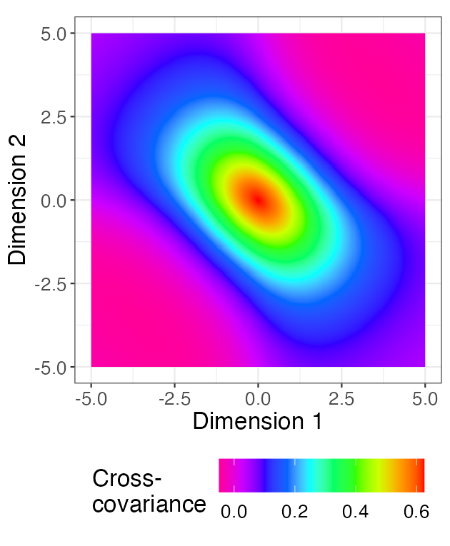
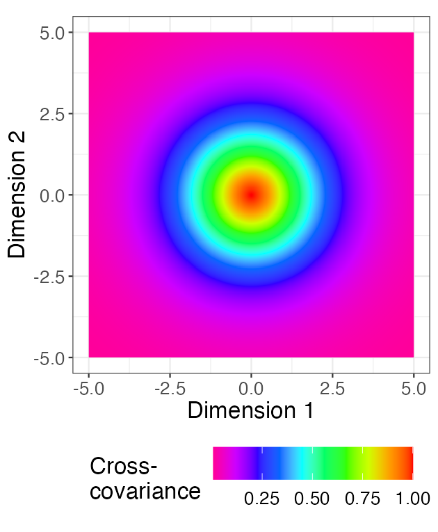
Figure 11: Matérn covariance functions with $d=2$, $\nu=1.5$, and $a=1$. (Left) With $\sigma(d\boldsymbol{\theta})=\mathbb{I}\left(\textrm{sign}(\theta_{1})=\textrm{sign}(\theta_{2})\right)+0.25\mathbb{I}\left(\textrm{sign}(\theta_{1})\neq\textrm{sign}(\theta_{2})\right)d\boldsymbol{\theta}$. (Right) With $\sigma(d\boldsymbol{\theta})=d\boldsymbol{\theta}$, resulting in the classical Matérn with unit variance.

We next turn to the multivariate case. In particular, we will demonstrate that the tangent processes of the multivariate Matérn processes $\boldsymbol{Y}(\boldsymbol{s})$ are operator fractional Brownian fields. Due to a one-to-one correspondence between the tangent processes of multivariate Matérn models and operator fractional Brownian fields (OFBFs), our proposed family of multivariate Matérn models succinctly are able to realize all possible local behavior of stationary vector-valued processes. We will revert to thinking of $\boldsymbol{\nu}$ as a real, symmetric, and positive-definite matrix that commutes with $\boldsymbol{a}$, rather than a diagonal matrix. As in Section 4, we interpret $\boldsymbol{A}^{\boldsymbol{B}}$ for two matrices as $\textrm{exp}(\boldsymbol{B}\log(\boldsymbol{A}))$ with $\log(\boldsymbol{A})$ defined for example through its Gregory series expansion in (4.1), for a diagonal matrix $\boldsymbol{A}$ with positive and bounded real parts of its eigenvalues; see again Cardoso and Sadeghi, (2018) and Barradas and Cohen, (1994).

E.2 Operator fractional Brownian fields

We next describe operator fractional Brownian fields, following Didier et al., (2018). Let $\boldsymbol{H}$ be a real, positive-definite $p\times p$ matrix, $\boldsymbol{E}$ be a real $d\times d$ matrix, and for all $c>0$ interpret $c^{\boldsymbol{H}}$ as $\exp\{\log(c)\boldsymbol{H}\}$, where the matrix exponent is defined as $\exp\{\boldsymbol{H}\}=\sum_{\ell=0}^{\infty}\boldsymbol{H}^{\ell}/\ell!$. Let $\boldsymbol{I}_{d}$ be the identity matrix of dimension $d\times d$. As in Didier et al., (2018), we consider matrices $\boldsymbol{H}$ and $\boldsymbol{E}$ with $0<\min\Re(\textrm{eig}(\boldsymbol{H}))\leq\max\Re(\textrm{eig}(\boldsymbol{H}))<\min\Re(\textrm{eig}(\boldsymbol{E}^{*}))=1$ without loss of generality, where $\textrm{eig}(\boldsymbol{A})$ denotes the eigenvalues of the matrix $\boldsymbol{A}$ and $\boldsymbol{E}^{*}$ is the conjugate transpose of $\boldsymbol{E}$. Switching the integrals to the polar coordinates of $r=\left\lVert\boldsymbol{x}\right\rVert$ and $\boldsymbol{\theta}=\boldsymbol{x}/\left\lVert\boldsymbol{x}\right\rVert\in\mathcal{S}^{d-1}$ where $\mathcal{S}^{d-1}$ is the unit sphere in $d-1$ dimensions, Remark 3.2 of Didier et al., (2018) represents an operator fractional Brownian field $\mathscr{B}(\boldsymbol{s})$ as

$$\begin{split}\{\mathscr{B}(\boldsymbol{s})\}_{\boldsymbol{s}\in\mathbb{R}^{d}}&\overset{fdd}{=}\Bigg{\{}\int_{0}^{\infty}\int_{\mathcal{S}^{d-1}}\left(e^{\mathbbm{i}\langle\boldsymbol{s},r^{\boldsymbol{E}^{*}}\boldsymbol{\theta}\rangle}-1\right)\\ &~{}~{}~{}~{}~{}\times r^{-\boldsymbol{H}-\frac{d}{2}\boldsymbol{I}_{p}}\boldsymbol{B}_{\boldsymbol{\mu}}(dr,d\boldsymbol{\theta})\Bigg{\}}_{\boldsymbol{s}\in\mathbb{R}^{d}},\end{split}$$ (E.10)

where $\overset{fdd}{=}$ denotes equality in finite-dimensional-distribution and $\boldsymbol{B}_{\boldsymbol{\mu}}(dr,d\boldsymbol{\theta})$ is a Hermitian Gaussian random measure with

$$\mathbb{E}\left[\boldsymbol{B}_{\boldsymbol{\mu}}(dr,d\boldsymbol{\theta})\boldsymbol{B}_{\boldsymbol{\mu}}(dr,d\boldsymbol{\theta})^{*}\right] =r^{d-1}dr\boldsymbol{\mu}(d\boldsymbol{\theta}).$$ (E.11)

(The slight difference in the form of the integrand in (E.10) above and that in Remark 3.2 of Didier et al., (2018) is due to the different control measure of $\boldsymbol{B}_{\boldsymbol{\mu}}(dr,d\boldsymbol{\theta})$ adopted in (E.11).) Here, $\boldsymbol{\mu}(d\boldsymbol{\theta})$ is a Hermitian measure on $\mathcal{S}^{d-1}$, i.e., such that $\boldsymbol{\mu}(d\boldsymbol{\theta})=\overline{\boldsymbol{\mu}(-d\boldsymbol{\theta})}$, which follows from the fact that the process $\mathscr{B}$ is real. Furthermore, we take $\boldsymbol{\mu}(d\boldsymbol{\theta})$ to be finite so that $\left\lVert\boldsymbol{\mu}(\mathcal{S}^{d-1})\right\rVert_{F}<\infty$ for the Frobenius norm $\lVert\cdot\rVert_{F}$. This characterizes the set of operator fractional Brownian fields; that is, this set contains all zero-mean, Gaussian, stationary-increment processes, which have the following $(\boldsymbol{H},\boldsymbol{E})$ operator self-similarity property. Namely, such that for all $c>0$

$$\left\{c^{\boldsymbol{H}}\mathscr{B}(\boldsymbol{s})\right\}_{\boldsymbol{s}\in\mathbb{R}^{d}}\overset{fdd}{=}\left\{\mathscr{B}\left(c^{\boldsymbol{E}}\boldsymbol{s}\right)\right\}_{\boldsymbol{s}\in\mathbb{R}^{d}}.$$ (E.12)

Remark E.6.

In the sequel, for simplicity, we will take $\boldsymbol{E}=\boldsymbol{I}_{d}$. Further flexibility could be achieved if general operator rescaling of the domain is adopted in the increments (E.1) appearing in the definition of tangent processes.

E.3 Multivariate tangent processes

Suppose now $\boldsymbol{Y}=\{\boldsymbol{Y}(\boldsymbol{s}),\ \boldsymbol{s}\in\mathbb{R}^{d}\}$ is a multivariate stochastic process taking values in $\mathbb{R}^{p}$ and consider the following natural generalization of Definition E.1. Namely, fix $\boldsymbol{s}_{0}$ and consider the increment processes

$$\boldsymbol{X}_{\epsilon}(\boldsymbol{s})=\boldsymbol{A}_{\epsilon}(\boldsymbol{Y}(\boldsymbol{s}_{0}+\epsilon\boldsymbol{s})-\boldsymbol{Y}(\boldsymbol{s}_{0}))$$ (E.13)

for $\epsilon>0$ and for a $p\times p$ matrix-valued function $\boldsymbol{A}_{\epsilon}$. A non-zero stochastic process $\boldsymbol{Z}=\{\boldsymbol{Z}(\boldsymbol{s})\}$ is said to be a tangent process to $\boldsymbol{Y}=\{\boldsymbol{Y}(\boldsymbol{s}),\ \boldsymbol{s}\in\mathbb{R}^{d}\}$ at $\boldsymbol{s}_{0}$ if

$$\left\{\boldsymbol{X}_{\epsilon}(\boldsymbol{s})\right\}_{\boldsymbol{s}\in\mathbb{R}^{d}}\overset{d}{\longrightarrow}\{\boldsymbol{Z}(\boldsymbol{s})\}_{\boldsymbol{s}\in\mathbb{R}^{d}}$$

as $\epsilon\downarrow 0$ for some choice of $\boldsymbol{A}_{\epsilon}$. As in the scalar case, the limiting process $\boldsymbol{Z}$ will have stationary increments and it will be self-similar. The self-similarity, however, is with respect to linear operator rescaling in the sense of (E.12) with some $p\times p$ matrix-valued exponent $\boldsymbol{H}$ and $\boldsymbol{E}=\boldsymbol{I}_{d}$.

We shall establish below the tangent process of the Matérn models for $\Re(\textrm{eig}(\boldsymbol{\nu}))\subset(0,1)$ when

$$\boldsymbol{A}_{\epsilon}:=\epsilon^{-\boldsymbol{\nu}}\boldsymbol{c}^{-1},$$ (E.14)

where the non-singular constant matrix $\boldsymbol{c}$ is in (4.3). To begin to characterize the resulting tangent process, we introduce Lemma E.7.

Lemma E.7.

Suppose that the matrices $\boldsymbol{a}$ and $\boldsymbol{\nu}$ in the definition of the multivariate Matérn model (4.3) commute. Then, the increments process (E.13) with $\boldsymbol{A}_{\epsilon}$ as in (E.14), can be characterized as follows

$$\boldsymbol{X}_{\epsilon}=\{\boldsymbol{X}_{\epsilon}(\boldsymbol{s})\}_{\boldsymbol{s}\in\mathbb{R}^{d}}$$

$$\overset{fdd}{=}\Bigg{\{}\int_{0}^{\infty}\int_{\mathcal{S}^{d-1}}\left(e^{\mathbbm{i}\langle\boldsymbol{s},r\boldsymbol{\theta}\rangle}-1\right)e^{\mathbbm{i}\langle\boldsymbol{s}_{0},\epsilon^{-1}r\boldsymbol{\theta}\rangle}$$

$$~{}~{}~{}~{}~{}~{}~{}~{}~{}~{}~{}~{}~{}~{}~{}~{}~{}~{}\times\left(\boldsymbol{a}\epsilon+\varphi(\boldsymbol{\theta})\mathbbm{i}r\boldsymbol{I}_{p}\right)^{-\boldsymbol{\nu}-\frac{d}{2}\boldsymbol{I}_{p}}\boldsymbol{B}_{\boldsymbol{\mu}}(dr,d\boldsymbol{\theta})\Bigg{\}}_{\boldsymbol{s}\in\mathbb{R}^{d}}.$$

Proof of Lemma E.7.

Throughout, we will use the fact that for a square matrix $\boldsymbol{A}$ of dimension $p$ and scalars $c$ and $b$, we have $b^{c}\boldsymbol{A}=\boldsymbol{A}b^{c}$. By (4.3), we have

$$\boldsymbol{X}_{\epsilon}(\boldsymbol{s}) =\epsilon^{-\boldsymbol{\nu}}\int_{0}^{\infty}\int_{\mathcal{S}^{d-1}}\left(e^{\mathbbm{i}\langle\epsilon\boldsymbol{s},r\boldsymbol{\theta}\rangle}-1\right)e^{\mathbbm{i}\langle\boldsymbol{s}_{0},r\boldsymbol{\theta}\rangle}$$

$$~{}~{}~{}~{}~{}~{}~{}~{}~{}~{}~{}\times(\boldsymbol{a}+\varphi(\boldsymbol{\theta})\mathbbm{i}r\boldsymbol{I}_{p})^{-\boldsymbol{\nu}-(d/2)\boldsymbol{I}_{p}}\boldsymbol{B}_{\boldsymbol{\mu}}(dr,d\boldsymbol{\theta}).$$

Then, in view of (4.2), making the change of variables $u=\epsilon r$, we obtain

$$\Big{\{}\boldsymbol{B}_{\boldsymbol{\mu}}(dr,d\boldsymbol{\theta})\Big{\}}\overset{fdd}{=}\Big{\{}\epsilon^{-\frac{d-1}{2}}\epsilon^{-\frac{1}{2}}\boldsymbol{B}_{\boldsymbol{\mu}}(du,d\boldsymbol{\theta})\Big{\}},$$

and hence

$$\{\boldsymbol{X}_{\epsilon}(\boldsymbol{s})\}\overset{fdd}{=}\Big{\{}\epsilon^{-\boldsymbol{\nu}}\int_{0}^{\infty}\int_{\mathcal{S}^{d-1}}\left(e^{\mathbbm{i}\langle\boldsymbol{s},u\boldsymbol{\theta}\rangle}-1\right)e^{\mathbbm{i}\langle\boldsymbol{s}_{0},\epsilon^{-1}u\boldsymbol{\theta}\rangle}$$

$$~{}~{}~{}~{}~{}~{}\times\left(\boldsymbol{a}+\varphi(\boldsymbol{\theta})\mathbbm{i}u\epsilon^{-1}\boldsymbol{I}_{p}\right)^{-\boldsymbol{\nu}-(d/2)\boldsymbol{I}_{p}}\epsilon^{-\frac{d}{2}}\boldsymbol{B}_{\boldsymbol{\mu}}(du,d\boldsymbol{\theta})\Big{\}}.$$

Next, we see that

$$\left(\boldsymbol{a}+\varphi(\boldsymbol{\theta})\mathbbm{i}u\epsilon^{-1}\boldsymbol{I}_{p}\right)^{-\boldsymbol{\nu}-(d/2)\boldsymbol{I}_{p}}$$

$$=\left(\epsilon^{-1}\left(\boldsymbol{a}\epsilon+\varphi(\boldsymbol{\theta})\mathbbm{i}u\boldsymbol{I}_{p}\right)\right)^{-\boldsymbol{\nu}-(d/2)\boldsymbol{I}_{p}}$$

$$=\epsilon^{\boldsymbol{\nu}+(d/2)\boldsymbol{I}_{p}}\left(\boldsymbol{a}\epsilon+\varphi(\boldsymbol{\theta})\mathbbm{i}u\boldsymbol{I}_{p}\right)^{-\boldsymbol{\nu}-(d/2)\boldsymbol{I}_{p}},$$

where we used the fact that since $\boldsymbol{\nu}\boldsymbol{a}=\boldsymbol{a}\boldsymbol{\nu}$ the matrices $\boldsymbol{a}\epsilon+\varphi(\boldsymbol{\theta})\mathbbm{i}u\boldsymbol{I}_{p}$ and $\boldsymbol{\nu}+(d/2)\boldsymbol{I}_{p}$ commute, so that the term $\epsilon^{\boldsymbol{\nu}+(d/2)\boldsymbol{I}_{p}}$ can be factored out. Here, we used the important fact that if $\boldsymbol{A}$ and $\boldsymbol{B}$ are commuting matrices and $\epsilon>0$, we have that $(\epsilon\boldsymbol{A})^{\boldsymbol{B}}=\epsilon^{\boldsymbol{B}}\boldsymbol{A}^{\boldsymbol{B}}$, whenever the matrix powers are well-defined.

Simplifying terms involving $\epsilon$, we see

$$\{\boldsymbol{X}_{\epsilon}(\boldsymbol{s})\} \overset{fdd}{=}\int_{0}^{\infty}\int_{\mathcal{S}^{d-1}}\left(e^{\mathbbm{i}\langle\boldsymbol{s},u\boldsymbol{\theta}\rangle}-1\right)e^{\mathbbm{i}\langle\boldsymbol{s}_{0},\epsilon^{-1}u\boldsymbol{\theta}\rangle}$$

$$\times\left(\boldsymbol{a}\epsilon+\varphi(\boldsymbol{\theta})\mathbbm{i}u\boldsymbol{I}_{p}\right)^{-\boldsymbol{\nu}-(d/2)\boldsymbol{I}_{p}}\boldsymbol{B}_{\boldsymbol{\mu}}(du,d\boldsymbol{\theta}),$$

the desired result. ∎

We next characterize the limit of $\boldsymbol{X}_{\epsilon}$, as $\epsilon\downarrow 0$. As anticipated from the scalar-valued case, the resulting tangent process is an operator fractional Brownian field. We focus on the important special case of $\Re(\textrm{eig}(\boldsymbol{\nu}))\subset(0,1)$.

Theorem E.8.

Let $\Re({{\textrm{eig}}}(\boldsymbol{\nu}))\subset(0,1)$, $\boldsymbol{a}$ and $\boldsymbol{\nu}$ commute, and $\{X_{\epsilon}(\boldsymbol{s})\}$ be the increments of the multivariate Matérn model introduced in (E.13) with $\boldsymbol{A}_{\epsilon}$ as in (E.14). Then, as $\epsilon\downarrow 0$, we have

$$\{\boldsymbol{X}_{\epsilon}(\boldsymbol{s})\}_{\boldsymbol{s}\in\mathbb{R}^{d}}$$

$$\overset{fdd}{\longrightarrow}\left\{\int_{0}^{\infty}\int_{\mathcal{S}^{d-1}}(e^{\mathbbm{i}\langle\boldsymbol{s},r\boldsymbol{\theta}\rangle}-1)r^{-\boldsymbol{\nu}-\frac{d}{2}\boldsymbol{I}_{p}}\boldsymbol{B}_{\tilde{\boldsymbol{\boldsymbol{\mu}}}}(dr,d\boldsymbol{\theta})\right\}_{\boldsymbol{s}\in\mathbb{R}^{d}},$$

where $\boldsymbol{B}_{\tilde{\boldsymbol{\mu}}}(dr,d\boldsymbol{\theta})$ is a complex Hermitian Gaussian random measure with orthogonal increments and control measure $\mathbb{E}\left[\boldsymbol{B}_{\tilde{\boldsymbol{\mu}}}(dr,d\boldsymbol{\theta})\boldsymbol{B}_{\tilde{\boldsymbol{\mu}}}(dr,d\boldsymbol{\theta})^{*}\right]=r^{d-1}dr\tilde{\boldsymbol{\mu}}(d\boldsymbol{\theta})$, with

$$\begin{split}&\tilde{\mu}(d\boldsymbol{\theta}):=e^{-\mathbbm{i}\pi\varphi(\boldsymbol{\theta})(\boldsymbol{\nu}+\frac{d}{2}\boldsymbol{I}_{p})}\mu(d\boldsymbol{\theta})e^{\mathbbm{i}\pi\varphi(\boldsymbol{\theta})(\boldsymbol{\nu}+\frac{d}{2}\boldsymbol{I}_{p})}.\end{split}$$ (E.15)

This form matches the characterization of OFBF in Didier et al., (2018). Therefore, the local properties of multivariate Matérn models presented here realize a large class of OFBFs that includes covariance-asymmetric processes.

Remark E.9.

Theorem (E.8) covers the important case when $\Re({{\textrm{eig}}}(\boldsymbol{\nu}))\subset(0,1)$. It can be shown that when $\Re(\textrm{eig}(\boldsymbol{\nu}))\subset[k,k+1)$ for $k\in\mathbb{N}$, the increments in (E.13) have trivial limits. Indeed, for $k\geq 1$, the process is mean-square differentiable and the tangent fields are simply random linear processes. In these cases, by considering higher order increments, one can obtain non-trivial higher-order tangent fields, which turn out to be intrinsically stationary in the sense of Matheron, (1973) (see, e.g., Chiles and Delfiner,, 2012; Shen et al.,, 2022). This analysis can be elegantly carried out using Matheron’s framework and the resulting $\lceil k\rceil$-th order tangent processes would be characterized by an operator-self-similar $\mathbb{R}^{p}$-valued intrinsic random function of order $k$. For more details, see Shen et al., (2022).

Remark E.10.

In order to achieve all possible tangent fields, one would choose $\boldsymbol{a}=a\boldsymbol{I}_{p}$ for $a>0$. In this setting, $\boldsymbol{a}$ and $\boldsymbol{\nu}$ commute, so that $\boldsymbol{\nu}$ may be a general real matrix such that $\Re({\rm eig}(\boldsymbol{\nu}))\subset(0,1)$. This shows that an arbitrary operator fractional Brownian motion with general matrix-valued Hurst exponent $\boldsymbol{H}=\boldsymbol{\nu}$ can arise as the tangent fields of a Matérn model. Notice that $\boldsymbol{a}$ does not appear in the process’s tangent field as it more directly describes the decay of the covariance rather than the local properties. However, in applications, for modeling flexibility, having different $a_{j}$ values for each process is important for modeling different ranges of dependence in the different coordinates of multivariate spatial models.

We now turn to the proof of Theorem E.8.

Proof of Theorem E.8.

Assuming Gaussianity, it is enough to show the convergence of the covariance function. From Equation (3.11) of Didier et al., (2018), we see that $\mathscr{B}(\boldsymbol{s})$ with such parameters has covariance

$$\begin{split}&\textrm{Cov}(\mathscr{B}(\boldsymbol{s}_{1}),\mathscr{B}(\boldsymbol{s}_{2}))\\ &~{}~{}~{}~{}~{}=\int_{0}^{\infty}\int_{\mathcal{S}^{d-1}}(e^{\mathbbm{i}\langle\boldsymbol{s}_{1},u\boldsymbol{\theta}\rangle}-1)(e^{-\mathbbm{i}\langle\boldsymbol{s}_{2},u\boldsymbol{\theta}\rangle}-1)\\ &~{}~{}~{}~{}~{}~{}~{}~{}\times u^{-\boldsymbol{\nu}}\tilde{\boldsymbol{\mu}}(d\boldsymbol{\theta})u^{-\boldsymbol{\nu}}u^{-1}du.\end{split}$$ (E.16)

Returning to our expression of $\{\boldsymbol{X}_{\epsilon}(\boldsymbol{s})\}$ in Lemma E.7, we see that

$$\begin{split}&\textrm{Cov}(\boldsymbol{X}_{\epsilon}(\boldsymbol{s}_{1}),\boldsymbol{X}_{\epsilon}(\boldsymbol{s}_{2}))\\ &=\int_{0}^{\infty}\int_{\mathcal{S}^{d-1}}(e^{\mathbbm{i}\langle\boldsymbol{s}_{1},u\boldsymbol{\theta}\rangle}-1)(e^{-\mathbbm{i}\langle\boldsymbol{s}_{2},u\boldsymbol{\theta}\rangle}-1)\\ &~{}~{}~{}~{}~{}~{}~{}~{}~{}\times(\boldsymbol{a}\epsilon+\varphi(\boldsymbol{\theta})\mathbbm{i}u\boldsymbol{I}_{p})^{-\boldsymbol{\nu}-\frac{d}{2}\boldsymbol{I}_{p}}\\ &~{}~{}~{}~{}~{}~{}~{}~{}~{}\times\mathbb{E}\left[\boldsymbol{B}_{\boldsymbol{\mu}}(du,d\boldsymbol{\theta})\boldsymbol{B}_{\boldsymbol{\mu}}(du,d\boldsymbol{\theta})^{*}\right]\\ &~{}~{}~{}~{}~{}~{}~{}~{}~{}\times(\boldsymbol{a}\epsilon-\varphi(\boldsymbol{\theta})\mathbbm{i}u\boldsymbol{I}_{p})^{-\boldsymbol{\nu}-\frac{d}{2}\boldsymbol{I}_{p}}.\end{split}$$ (E.17)

First, we can straightforwardly evaluate the limit inside the integral:

$$\lim_{\epsilon\downarrow 0} (\boldsymbol{a}\epsilon+\varphi(\boldsymbol{\theta})\mathbbm{i}u\boldsymbol{I}_{p})^{-\boldsymbol{\nu}-\frac{d}{2}\boldsymbol{I}_{p}}\mathbb{E}\left[\boldsymbol{B}_{\boldsymbol{\mu}}(du,d\boldsymbol{\theta})\boldsymbol{B}_{\boldsymbol{\mu}}(du,d\boldsymbol{\theta})^{*}\right]$$

$$~{}~{}~{}~{}~{}~{}~{}~{}~{}~{}~{}~{}\times(\boldsymbol{a}\epsilon-\varphi(\boldsymbol{\theta})\mathbbm{i}u\boldsymbol{I}_{p})^{-\boldsymbol{\nu}-\frac{d}{2}\boldsymbol{I}_{p}}$$

$$=(\varphi(\boldsymbol{\theta})\mathbbm{i}u\boldsymbol{I}_{p})^{-\boldsymbol{\nu}-\frac{d}{2}\boldsymbol{I}_{p}}\mathbb{E}\left[\boldsymbol{B}_{\boldsymbol{\mu}}(du,d\boldsymbol{\theta})\boldsymbol{B}_{\boldsymbol{\mu}}(du,d\boldsymbol{\theta})^{*}\right]$$

$$~{}~{}~{}~{}~{}~{}~{}~{}~{}~{}~{}~{}\times(-\varphi(\boldsymbol{\theta})\mathbbm{i}u\boldsymbol{I}_{p})^{-\boldsymbol{\nu}-\frac{d}{2}\boldsymbol{I}_{p}}$$

$$=u^{-\boldsymbol{\nu}-\frac{d}{2}\boldsymbol{I}_{p}}\mathbb{E}\Big{[}e^{\mathbbm{i}\pi\varphi(\boldsymbol{\theta})(-\boldsymbol{\nu}-\frac{d}{2}\boldsymbol{I}_{p})/2}\boldsymbol{B}_{\boldsymbol{\mu}}(du,d\boldsymbol{\theta})$$

$$~{}~{}~{}~{}~{}~{}~{}~{}~{}~{}~{}~{}\times\boldsymbol{B}_{\boldsymbol{\mu}}(du,d\boldsymbol{\theta})^{*}e^{-\mathbbm{i}\pi\varphi(\boldsymbol{\theta})(-\boldsymbol{\nu}-\frac{d}{2}\boldsymbol{I}_{p})/2}\Big{]}$$

$$~{}~{}~{}~{}~{}~{}~{}~{}~{}~{}~{}~{}\times u^{-\boldsymbol{\nu}-\frac{d}{2}\boldsymbol{I}_{p}}.$$

Now, using the definition of $\tilde{\boldsymbol{\mu}}$ in (LABEL:e:mu-tilde), we see that

$$\mathbb{E}\Big{[}e^{\mathbbm{i}\pi\varphi(\boldsymbol{\theta})(-\nu-\frac{d}{2}\boldsymbol{I}_{p})/2}\boldsymbol{B}_{\boldsymbol{\mu}}(du,d\boldsymbol{\theta})\boldsymbol{B}_{\boldsymbol{\mu}}(du,d\boldsymbol{\theta})^{*}$$

$$~{}~{}~{}~{}~{}~{}\times e^{-\mathbbm{i}\pi\varphi(\boldsymbol{\theta})(-\boldsymbol{\nu}-\frac{d}{2}\boldsymbol{I}_{p})/2}\Big{]}=u^{d-1}du\tilde{\boldsymbol{\mu}}(d\boldsymbol{\theta}).$$

Therefore, provided we can justify the exchange of limits and integration, we have

$$\lim_{\epsilon\downarrow 0}\textrm{Cov}(\boldsymbol{X}_{\epsilon}(\boldsymbol{s}_{1}),\boldsymbol{X}_{\epsilon}(\boldsymbol{s}_{2}))$$

$$=\int_{0}^{\infty}\int_{\mathcal{S}^{d-1}}(e^{\mathbbm{i}\langle\boldsymbol{s}_{1},u\boldsymbol{\theta}\rangle}-1)(e^{-\mathbbm{i}\langle\boldsymbol{s}_{2},u\boldsymbol{\theta}\rangle}-1)$$

$$~{}~{}~{}~{}~{}~{}~{}~{}~{}~{}~{}~{}~{}~{}~{}~{}~{}~{}~{}~{}~{}u^{-\boldsymbol{\nu}}\tilde{\boldsymbol{\mu}}(d\boldsymbol{\theta})u^{-\boldsymbol{\nu}}u^{-1}du,$$

matching the covariance of the OFBF in (LABEL:e:Cov-OFBM), which is well-defined since $\Re(\textrm{eig}(\boldsymbol{\nu}))\subset(0,1)$.

To complete the proof, we will next justify the exchange of the limit and integration by using the dominated convergence theorem. Note that all integrals involving matrix-valued functions and measures are in fact component-wise integrals with respect to signed measures. However, conceptually, it will be convenient to view integration with respect to a measure $\boldsymbol{\mu}(\cdot)$ taking values in the space of positive semidefinite matrices (see also Shen et al.,, 2022). In this case a ($p\times p$-matrix-valued) function $(u,\boldsymbol{\theta})\mapsto G(u,\boldsymbol{\theta})$ is integrable with respect to $\boldsymbol{\mu}$, provided

$$\int_{0}^{\infty}\int_{\mathcal{S}^{d-1}}\|G(u,\boldsymbol{\theta})\|du\|\boldsymbol{\mu}\|(d\boldsymbol{\theta})<\infty,$$

where $\|\boldsymbol{A}\|:={\rm trace}((\boldsymbol{A}^{*}\boldsymbol{A})^{1/2})$ is the trace matrix norm. Here, $\|\boldsymbol{\mu}\|(d\boldsymbol{\theta}):=\|\boldsymbol{\mu}(d\boldsymbol{\theta})\|$ is a finite (scalar) measure on $\mathcal{S}^{d-1}$, defined by letting $\|\mu\|(B):=\|\mu(B)\|$, for all measurable $B\subset\mathcal{S}^{d-1}.$ To see that $\|\boldsymbol{\mu}\|$ is a valid measure, observe that for disjoint measurable sets $B,C\subset\mathcal{S}^{d-1},$ we have that the matrices $\boldsymbol{\mu}(B)$ and $\boldsymbol{\mu}(C)$ are positive semidefinite. Hence, for $\boldsymbol{\mu}(B\cup C)=\boldsymbol{\mu}(B)+\boldsymbol{\mu}(C)$, we have

$$\|\boldsymbol{\mu}(B\cup C)\| ={\rm trace}(\boldsymbol{\mu}(B)+\boldsymbol{\mu}(C))$$

$$={\rm trace}(\boldsymbol{\mu}(B))+{\rm trace}(\boldsymbol{\mu}(C))$$

$$=\|\boldsymbol{\mu}(B)\|+\|\boldsymbol{\mu}(C)\|,$$

proving the additivity of $\|\boldsymbol{\mu}(\cdot)\|$. The $\sigma$-additivity of $\|\boldsymbol{\mu}(\cdot)\|$ follows similarly from the $\sigma$-additivity of $\boldsymbol{\mu}(\cdot)$ (Shen et al.,, 2022).

Now, turning to the integrand in (E.17), we have that

$$\left\lVert(\boldsymbol{a}\epsilon+\varphi(\boldsymbol{\theta})\mathbbm{i}u)^{-\boldsymbol{\nu}-d/2\boldsymbol{I}_{p}}(\boldsymbol{a}\epsilon-\varphi(\boldsymbol{\theta})\mathbbm{i}u\boldsymbol{I}_{p})^{-\boldsymbol{\nu}-d/2\boldsymbol{I}_{p}}\right\rVert_{\textrm{}}$$

$$~{}~{}~{}~{}~{}~{}~{}~{}~{}~{}~{}~{}~{}~{}~{}~{}=\left\lVert\left(\boldsymbol{a}^{2}\epsilon^{2}+u^{2}\boldsymbol{I}_{p}\right)^{-\boldsymbol{\nu}-d/2\boldsymbol{I}_{p}}\right\rVert_{\textrm{}},$$

which we will now show is integrable uniformly in $\epsilon>0$, using a similar approach as in the proof of Lemma D.1. Specifically, we want to examine

$$\int_{0}^{\infty}\int_{\mathcal{S}^{d-1}}\left|\left(e^{\mathbbm{i}\langle\boldsymbol{s}_{1},u\boldsymbol{\theta}\rangle}-1\right)\left(e^{-\mathbbm{i}\langle\boldsymbol{s}_{2},u\boldsymbol{\theta}\rangle}-1\right)\right|$$

$$~{}~{}~{}~{}~{}~{}\times\left\lVert(\boldsymbol{a}^{2}\epsilon^{2}+u^{2}\boldsymbol{I}_{p})^{-\boldsymbol{\nu}-(d/2)\boldsymbol{I}_{p}}\right\rVert_{\textrm{}}u^{d-1}du\left\lVert\boldsymbol{\mu}\right\rVert_{\textrm{}}(d\boldsymbol{\theta}),$$

and show that the integrand is bounded (uniformly in $\epsilon>0$) by a measurable non-negative function $g(u,\boldsymbol{\theta})$ such that

$$\int_{0}^{\infty}\int_{\mathcal{S}^{d-1}}g(u,\boldsymbol{\theta})du\left\lVert\boldsymbol{\mu}\right\rVert_{\textrm{}}(d\boldsymbol{\theta})<\infty.$$

Observe that, for all $x\in\mathbb{R}$, we have

$$|e^{\mathbbm{i}x}-1|^{2}=2(1-\cos(x))\leq\min\{4,\,x^{2}\}.$$

Indeed, the last inequality follows by observing that the function $x\mapsto x^{2}+2(\cos(x)-1)$ is non-negative for all $x\in\mathbb{R}$. This implies that

$$\left|\left(e^{\mathbbm{i}\langle\boldsymbol{s}_{1},u\boldsymbol{\theta}\rangle}-1\right)\left(e^{-\mathbbm{i}\langle\boldsymbol{s}_{2},u\boldsymbol{\theta}\rangle}-1\right)\right|$$

$$~{}~{}~{}~{}\leq\min\{4,(\|\boldsymbol{s}_{1}\|^{2}\vee\|\boldsymbol{s}_{2}\|^{2})\cdot u^{2}\}\leq 4\wedge(C_{\boldsymbol{s}_{1},\boldsymbol{s}_{2}}\cdot u^{2}),$$

where $C_{\boldsymbol{s}_{1},\boldsymbol{s}_{2}}=\|\boldsymbol{s}_{1}\|^{2}\vee\|\boldsymbol{s}_{2}\|^{2}$, $a\vee b=\textrm{max}\{a,b\}$, $a\wedge b=\textrm{min}\{a,b\}$, and we used the fact that $|\langle\boldsymbol{s}_{i},u\boldsymbol{\theta}\rangle|\leq\|\boldsymbol{s}_{i}\|\cdot|u|$ for all $\boldsymbol{\theta}\in\mathcal{S}^{d-1}$. We turn our attention to

$$\left\lVert\left(\boldsymbol{a}^{2}\epsilon^{2}+u^{2}\boldsymbol{I}_{p}\right)^{-\boldsymbol{\nu}-(d/2)\boldsymbol{I}_{p}}\right\rVert_{\textrm{}}$$

$$~{}~{}~{}~{}~{}\leq p\times\left\lVert\left(\boldsymbol{a}^{2}\epsilon^{2}+u^{2}\boldsymbol{I}_{p}\right)^{-\boldsymbol{\nu}-(d/2)\boldsymbol{I}_{p}}\right\rVert_{\textrm{op}},$$

where $\|\boldsymbol{A}\|_{{\rm op}}:=\sup_{\boldsymbol{x}\not=\boldsymbol{0}}\|\boldsymbol{A}\boldsymbol{x}\|/\|\boldsymbol{x}\|$ stands for the operator matrix norm induced by the Euclidean norm in $\mathbb{R}^{p}$. As the real parts of the eigenvalues in the exponent are non-negative,

$$\left\lVert\left(\boldsymbol{a}^{2}\epsilon^{2}+u^{2}\boldsymbol{I}_{p}\right)^{-\boldsymbol{\nu}-(d/2)\boldsymbol{I}_{p}}\right\rVert_{\textrm{op}} \leq\left\lVert\left(u^{2}\boldsymbol{I}_{p}\right)^{-\boldsymbol{\nu}-(d/2)\boldsymbol{I}_{p}}\right\rVert_{\textrm{op}}$$

$$\leq\left\lVert u^{-2\boldsymbol{\nu}-d\boldsymbol{I}_{p}}\right\rVert_{\textrm{op}}$$

(see also Relation (5.20) in Shen et al.,, 2020). This step requires that the matrices $\boldsymbol{a}$ and $\boldsymbol{\nu}$ are positive-definite and commute, so that they may be simultaneously diagonalized with the inequalities may straightforwardly take effect in this diagonalized space. From here, we see that

$$\left\lVert u^{-2\boldsymbol{\nu}-d\boldsymbol{I}_{p}}\right\rVert_{\textrm{op}} =u^{-2\min\{\textrm{eig}(\boldsymbol{\nu})\}-d}.$$

Therefore, we have the bound

$$\int_{0}^{\infty}\int_{\mathcal{S}^{d-1}}\left|\left(e^{\mathbbm{i}\langle\boldsymbol{s},u\boldsymbol{\theta}\rangle}-1\right)\left(e^{-\mathbbm{i}\langle\boldsymbol{s}_{2},u\boldsymbol{\theta}\rangle}-1\right)\right|$$

$$~{}~{}~{}~{}~{}~{}\times\left\lVert(\boldsymbol{a}^{2}\epsilon^{2}+u^{2}\boldsymbol{I}_{p})^{-\boldsymbol{\nu}-(d/2)\boldsymbol{I}_{p}}\right\rVert_{\textrm{op}}u^{d-1}\left\lVert\boldsymbol{\mu}\right\rVert_{F}(d\boldsymbol{\theta})du$$

$$~{}~{}~{}~{}~{}\leq\int_{0}^{\infty}\int_{\mathcal{S}^{d-1}}4u^{-2\min\{\textrm{eig}(\boldsymbol{\nu})\}-1}\left\lVert\boldsymbol{\mu}\right\rVert_{F}(d\boldsymbol{\theta})du,$$

which, with respect to $u$, is integrable for large $u$ when $-2\min\{\textrm{eig}(\boldsymbol{\nu})\}-1<-1$, or equivalently, $\min\{\textrm{eig}(\boldsymbol{\nu})\}>0$. If the matrix $\boldsymbol{\nu}$ is diagonal, the restriction $\min\{\textrm{eig}(\boldsymbol{\nu})\}>0$ is equivalent to having all diagonal entries satisfying $\nu_{k}>0$, as expected. For small $u$, we can make the bound

$$\int_{0}^{\infty}\int_{\mathcal{S}^{d-1}}\left|\left(e^{\mathbbm{i}\langle\boldsymbol{s},u\boldsymbol{\theta}\rangle}-1\right)\left(e^{-\mathbbm{i}\langle\boldsymbol{s}_{2},u\boldsymbol{\theta}\rangle}-1\right)\right|$$

$$~{}~{}~{}~{}~{}~{}\times\left\lVert(\boldsymbol{a}^{2}\epsilon^{2}+u^{2}\boldsymbol{I}_{p})^{-\boldsymbol{\nu}-(d/2)\boldsymbol{I}_{p}}\right\rVert_{\textrm{op}}u^{d-1}\left\lVert\boldsymbol{\mu}\right\rVert_{F}(d\boldsymbol{\theta})du$$

$$~{}~{}~{}~{}~{}\leq C_{\boldsymbol{s}_{1},\boldsymbol{s}_{2}}\int_{0}^{\infty}\int_{\mathcal{S}^{d-1}}u^{1-2\min\{\textrm{eig}(\boldsymbol{\nu})\}}\left\lVert\boldsymbol{\mu}\right\rVert(d\boldsymbol{\theta})du.$$

The is integrable with respect to $u$ for small $u$ when $1-2\min\{\textrm{eig}(\boldsymbol{\nu})\}>-1$, requiring $\min{\textrm{eig}(\boldsymbol{\nu})}<1$, which is done by assumption. Thus, the integral across all $u\in(0,\infty)$ is integrable. Finally, by using the linearity property of the trace, it remains to establish that $\left\lVert\boldsymbol{\mu}(\mathcal{S}^{d-1})\right\rVert<\infty$, which follows from the assumed properties of $\boldsymbol{\mu}(d\boldsymbol{\theta})$. Therefore, the integrand is dominated by an integrable function, and we may exchange the limit $\epsilon\to 0$ and integration. ∎

Appendix F Schoenberg’s representation of the classical Matérn covariance

The advantages and features of the classical Matérn covariance functions have been widely recognized in the statistics community and beyond. See, for example the monograph Stein, (1999) and the recent comprehensive review Porcu et al., (2023). Here, we shall present yet another perspective to the classical Matérn models and also provide an intuitive derivation of (1.5) from (1.4). See also Cho et al., (2017).

The utility of the Matérn covariance models

$${\cal M}(h;a,\nu,\sigma^{2})=\sigma^{2}\frac{2^{1-\nu}}{\Gamma(\nu)}(ah)^{\nu}{\cal K}_{\nu}(ah)$$

has long been recognized in spatial statistics. The inverse range parameter $a$ and the regularity exponent $\nu$ allow for a great flexibility in modeling local dependence as well as the path roughness property of the underlying stochastic process $Y=\{Y(\boldsymbol{t}),\ \boldsymbol{t}\in\mathbb{R}^{d}\}$. Another, notable feature of the classical Matérn covariance

$$\mathbb{E}[Y(\boldsymbol{t}+\boldsymbol{h})Y(\boldsymbol{t})]=C_{Y}(\|\boldsymbol{h}\|)={\cal M}(\|\boldsymbol{h}\|;a,\nu,\sigma^{2})$$

for $\boldsymbol{h},\boldsymbol{t}\in\mathbb{R}^{d}$, is that it is isotropic and the function $C_{Y}:\mathbb{R}\to\mathbb{R}$ is such that $\boldsymbol{h}\mapsto C_{Y}(\|\boldsymbol{h}\|)$ is positive semidefinite, in all dimensions $d\geq 1$, where $\|\cdot\|$ stands for the Euclidean norm in $\mathbb{R}^{d}$. This dimension-free positivity property is rather special and convenient since one does not need to specify (or even know!) the dimension $d$ of the underlying space. Indeed, suppose that we have a collection of points $x_{i},\ i=1,\cdots,n$ equipped with a metric $\rho(x_{i},x_{j})$. So long as the metric is embeddable in an Euclidean space, i.e., for some $d\geq 1$, there exist $\boldsymbol{t}_{i}\in\mathbb{R}^{d}$, such that $\rho(x_{i},x_{j})=\|\boldsymbol{t}_{i}-\boldsymbol{t}_{j}\|,\ i,j=1,\cdots,d$, then the matrix $C:=(C_{Y}(\rho(x_{i},x_{j})))_{n\times n}$ is a valid covariance matrix. Hence, if one has a process $\{Y(x),\ x\in{\cal X}\}$ over an arbitrary index set, so long as the underlying distance structure on ${\cal X}$ is embeddable in an Euclidean space, one can model the covariance structure of $Y(x_{i}),\ i=1,\cdots,n$ with Matérn. This is particularly appealing in spatial statistics applications, where one can do kriging for example in the same way in all dimensions.

Fundamental problems on the embeddability of metric spaces in Hilbert spaces and related questions have been studies by Schoenberg. Specifically, a result due to Schoenberg, (1938) characterized the class of continuous functions $\varphi:[0,\infty)\to\mathbb{R}$ such that $\boldsymbol{h}\mapsto\varphi(\|\boldsymbol{h}\|),\ \boldsymbol{h}\in\mathbb{R}^{d}$ is positive semidefinite for all dimensions $d\geq 1$, where $\|\cdot\|$ stands for the Euclidean norm. Namely, they are precisely variance mixtures of Gaussian kernels:

$$\varphi(x)=\int_{0}^{\infty}e^{-x^{2}u}\mu(du),$$

for some finite measure $\mu$ on $[0,\infty)$ (Schoenberg,, 1938, Theorem 2).

This characterization calls for the natural question as to what is the measure $\mu$ in the Schoenberg representation of the Matérn covariance. Using the integral representation (10.32.10) of ${\cal K}_{\nu}$ in DLMF, (2021), with the change of variables $u:=z^{2}u$ therein, or equivalently Theorem 1.1 in Cho et al., (2017) one obtains:

$$\begin{split}{\cal M}(z;1,\nu,1)&\equiv\frac{2^{1-\nu}}{\Gamma(\nu)}z^{\nu}{\cal K}_{\nu}(z)\\ &=\int_{0}^{\infty}e^{-z^{2}u}g_{\nu}(u)du,\end{split}$$ (F.1)

where $g_{\nu}(u)=u^{-\nu-1}e^{-1/(4u)}/(2^{2\nu}\Gamma(\nu)),\ u>0$ is the density of an inverse Gamma probability distribution. Namely, $g_{\nu}$ is the probability density of the random variable $1/X$, where $X\sim{\rm Gamma}(\nu,1/4)$.

Let $f_{d,(1,\nu,1)}(\boldsymbol{x})=:f_{d,\nu}(\boldsymbol{x})$ be the spectral density corresponding to the Matérn autocovariance ${\cal M}(\|\boldsymbol{h}\|;1,\nu,1)$, where for simplicity and without loss of generality, we will consider the standard Matérn model with $a=\sigma^{2}=1$. That is,

$${\cal M}(\|\boldsymbol{h}\|;1,\nu,1)=\int_{\mathbb{R}^{d}}e^{\mathbbm{i}\langle\boldsymbol{h},\boldsymbol{x}\rangle}f_{d,\nu}(\boldsymbol{x})dx.$$

The following result establishes the form of the spectral density $f_{d,\nu}$, from which the proof that (1.4) implies (1.5) readily follows with a change of variables.

Proposition F.1.

For $\boldsymbol{x}\in\mathbb{R}^{d}$, we have that

$$f_{d,(1,\nu,1)}(\boldsymbol{x})=\frac{\Gamma(\nu+d/2)}{\pi^{d/2}\Gamma(\nu)}\frac{1}{(1+\|\boldsymbol{x}\|^{2})^{\nu+d/2}}.$$ (F.2)

Remark F.2.

Notice that the marginal variance of the standard Matérn equals $1$. This implies that its spectral density integrates to $1$ and hence it can be interpreted as a probability density. In particular, the standard Matérn spectral density in (F.2) is the density of the multivariate t-distribution in $\mathbb{R}^{d}$ with parameters $\Sigma=(2\nu)^{-1}\mathbb{I}_{d}$ and degrees of freedom parameter $2\nu$.

Proof of Proposition F.1.

By the Fourier inversion theorem and the Schoenberg representation (F.1), we have that

$$f_{d,(1,\nu,1)}(\boldsymbol{x})=\frac{1}{(2\pi)^{d}}\int_{\mathbb{R}^{d}}e^{-\mathbbm{i}\langle\boldsymbol{x},\boldsymbol{h}\rangle}{\cal M}(\boldsymbol{x};1,\nu,1)d\boldsymbol{h}$$

$$~{}~{}~{}~{}=\int_{0}^{\infty}\left(\frac{1}{(2\pi)^{d}}\int_{\mathbb{R}^{d}}e^{-\|\boldsymbol{x}\|^{2}u}e^{-\mathbbm{i}\langle\boldsymbol{x},\boldsymbol{h}\rangle}d\boldsymbol{h}\right)g_{\nu}(u)du,$$

where in the last relation we applied Fubini’s theorem. Observe that the inner integral, with the multiplicative constant, is precisely the inverse Fourier transform of the characteristic function of a zero-mean Gaussian distribution in $\mathbb{R}^{d}$ with covariance matrix $\Sigma=2u\cdot\mathbb{I}_{d}$. Therefore,

$$f_{d,(1,\nu,1)}(\boldsymbol{x}) =\frac{1}{2^{2\nu}\Gamma(\nu)}\int_{0}^{\infty}\frac{1}{(4\pi u)^{d/2}}e^{-\|\boldsymbol{x}\|^{2}/(4u)}$$

$$~{}~{}~{}~{}~{}~{}~{}~{}~{}~{}~{}~{}~{}~{}~{}~{}~{}~{}~{}~{}~{}~{}~{}~{}~{}~{}~{}~{}~{}~{}\times u^{-\nu-1}e^{-1/(4u)}du$$

$$=\frac{1}{\pi^{d/2}2^{2\nu+d}\Gamma(\nu)}\int_{0}^{\infty}e^{-(\|\boldsymbol{x}\|^{2}+1)/(4u)}$$

$$~{}~{}~{}~{}~{}~{}~{}~{}~{}~{}~{}~{}~{}~{}~{}~{}~{}~{}~{}~{}~{}~{}~{}~{}~{}~{}~{}~{}~{}~{}\times u^{-(d/2+\nu+1)}du$$

$$=\frac{(1+\|\boldsymbol{x}\|^{2})^{-\nu-\frac{d}{2}}}{\pi^{d/2}2^{2\nu}\Gamma(\nu)}\int_{0}^{\infty}e^{-\frac{1}{4t}}t^{-(\nu+\frac{d}{2}+1)}dt$$ (F.3)

$$=\frac{\Gamma(\nu+d/2)2^{2\nu+d}}{\pi^{d/2}2^{2\nu+d}\Gamma(\nu)}\cdot\frac{1}{(1+\|\boldsymbol{x}\|^{2})^{\nu+\frac{d}{2}}},$$ (F.4)

where Relation (F.3) follows by making the change of variables $t:=u/(1+\|\boldsymbol{x}\|)$ and (F.4), from the observation that the integrand in (F.3) is up to a constant, the density of an inverse Gamma law with parameters $\nu+d/2$ and $1/4$. Relation (F.4) equals (F.2). ∎

References

- Abramowitz and Stegun, (1972) Abramowitz, M. and Stegun, I. A. (1972). Handbook of Mathematical Functions: With Formulas, Graphs and Mathematical Tables. Dover, New York.
- Agrest and Maksimov, (1971) Agrest, M. M. and Maksimov, M. S. (1971). Theory of Incomplete Cylindrical Functions and their Applications. Springer, Berlin, Heidelberg.
- Alegría et al., (2021) Alegría, A., Emery, X., and Porcu, E. (2021). Bivariate Matérn covariances with cross-dimple for modeling coregionalized variables. Spatial Statistics.
- Apanasovich and Genton, (2010) Apanasovich, T. V. and Genton, M. G. (2010). Cross-covariance functions for multivariate random fields based on latent dimensions. Biometrika, 97(1):15–30.
- Apanasovich et al., (2012) Apanasovich, T. V., Genton, M. G., and Sun, Y. (2012). A valid Matérn class of cross-covariance functions for multivariate random fields with any number of components. Journal of the American Statistical Association, 107(497):180–193.
- Argo, (2020) Argo (2020). Argo float data and metadata from Global Data Assembly Centre (Argo GDAC).
- Averbuch et al., (2006) Averbuch, A., Coifman, R., Donoho, D., Elad, M., and Israeli, M. (2006). Fast and accurate Polar Fourier transform. Applied and Computational Harmonic Analysis, 21(2):145–167.
- Babister, (1967) Babister, A. W. (1967). Transcendental Functions Satisfying Nonhomogeneous Linear Differential Equations. Macmillan, New York.
- Barradas and Cohen, (1994) Barradas, I. and Cohen, J. (1994). Iterated exponentiation, matrix-matrix exponentiation, and entropy. Journal of Mathematical Analysis and Applications, 183(1):76–88.
- Bochner, (1948) Bochner, S. (1948). Vorlesungen über Fouriersche integrale. Chelsea Publishing Company.
- Bolin and Wallin, (2019) Bolin, D. and Wallin, J. (2019). Multivariate type G Matérn stochastic partial differential equation random fields. Journal of the Royal Statistical Society: Series B (Statistical Methodology).
- Byrd et al., (1995) Byrd, R. H., Lu, P., Nocedal, J., and Zhu, C. (1995). A limited memory algorithm for bound constrained optimization. SIAM Journal on Scientific Computing, 16(5):1190–1208.
- Cardoso and Sadeghi, (2018) Cardoso, J. R. and Sadeghi, A. (2018). Conditioning of the matrix-matrix exponentiation. Numerical Algorithms, 79(2):457–477.
- Chiles and Delfiner, (2012) Chiles, J.-P. and Delfiner, P. (2012). Geostatistics: Modeling Spatial Uncertainty, volume 713. John Wiley & Sons.
- Cho et al., (2017) Cho, Y.-K., Kim, D., Park, K., and Yun, H. (2017). Schoenberg representations and Gramian matrices of Matérn functions.
- Cooley and Tukey, (1965) Cooley, J. W. and Tukey, J. W. (1965). An algorithm for the machine calculation of complex Fourier series. Mathematics of Computation, 19(90):297–301.
- Cramér, (1942) Cramér, H. (1942). On harmonic analysis in certain functional spaces.
- Cressie and Zammit-Mangion, (2016) Cressie, N. and Zammit-Mangion, A. (2016). Multivariate spatial covariance models: a conditional approach. Biometrika, 103(4):915–935.
- Didier et al., (2018) Didier, G., Meerschaert, M. M., and Pipiras, V. (2018). Domain and range symmetries of operator fractional Brownian fields. Stochastic Processes and their Applications, 128(1):39–78.
- Didier and Pipiras, (2011) Didier, G. and Pipiras, V. (2011). Integral representations and properties of operator fractional Brownian motions. Bernoulli, 17(1):1–33.
- Dingle, (1959) Dingle, R. B. (1959). Asymptotic expansions and converging factors. v. lommel, struve, modified struve, anger and weber functions, and integrals of ordinary and modified bessel functions. Proceedings of the Royal Society of London. Series A, Mathematical and Physical Sciences, 249(1257):284–292.
- DLMF, (2021) DLMF (2021). NIST Digital Library of Mathematical Functions. http://dlmf.nist.gov/, Release 1.1.3 of 2021-09-15. F. W. J. Olver, A. B. Olde Daalhuis, D. W. Lozier, B. I. Schneider, R. F. Boisvert, C. W. Clark, B. R. Miller, B. V. Saunders, H. S. Cohl, and M. A. McClain, eds.
- Durand and Roueff, (2022) Durand, A. and Roueff, F. (2022). Weakly stationary stochastic processes valued in a separable Hilbert space: Gramian-Cramér representations and applications.
- Emery et al., (2016) Emery, X., Arroyo, D., and Porcu, E. (2016). An improved spectral turning-bands algorithm for simulating stationary vector Gaussian random fields. Stochastic Environmental Research and Risk Assessment, 30(7):1863–1873.
- Emery et al., (2022) Emery, X., Porcu, E., and White, P. (2022). New validity conditions for the multivariate Matérn coregionalization model, with an application to exploration geochemistry. Mathematical Geosciences.
- Fahmy and Guinness, (2022) Fahmy, Y. and Guinness, J. (2022). Vecchia approximations and optimization for multivariate Matérn models. Journal of Data Science, pages 475–492.
- Falconer, (2002) Falconer, K. J. (2002). Tangent fields and the local structure of random fields. Journal of Theoretical Probability, 15:731–750.
- Falconer, (2003) Falconer, K. J. (2003). The local structure of random processes. Journal of the London Mathematical Society, 67:657–672.
- Fischer et al., (2023) Fischer, A., Gaunt, R. E., and Sarantsev, A. (2023). The variance-gamma distribution: a review. arXiv:2303.05615.
- Frigo, (1999) Frigo, M. (1999). A fast Fourier transform compiler. ACM SIGPLAN Notices, 34(5):169–180.
- Gelfand and Banerjee, (2010) Gelfand, A. and Banerjee, S. (2010). Multivariate spatial process models. In Gelfand, A., Diggle, P., Fuentes, M., and Guttorp, P., editors, Handbook of Spatial Statistics, volume 20103158, pages 495–515. CRC Press.
- Genton and Kleiber, (2015) Genton, M. G. and Kleiber, W. (2015). Cross-covariance functions for multivariate geostatistics. Statistical Science, 30(2):147–163.
- Gneiting et al., (2010) Gneiting, T., Kleiber, W., and Schlather, M. (2010). Matérn cross-covariance functions for multivariate random fields. Journal of the American Statistical Association, 105(491):1167–1177.
- Goulet, (2016) Goulet, V. (2016). expint: Exponential Integral and Incomplete Gamma Function. R package.
- Gradshteyn et al., (2015) Gradshteyn, I., Ryzhik, I., Zwillinger, D., and Moll, V., editors (2015). Table of Integrals, Series, and Products. Academic Press, Amsterdam.
- Guinness, (2022) Guinness, J. (2022). Nonparametric spectral methods for multivariate spatial and spatial–temporal data. Journal of Multivariate Analysis, 187:104823.
- Hannan, (1970) Hannan, E. (1970). Multiple Time Series. Springer-Verlag, New York.
- Hančová et al., (2022) Hančová, M., Gajdoš, A., and Hanč, J. (2022). A practical, effective calculation of gamma difference distributions with open data science tools. Journal of Statistical Computation and Simulation, pages 1–28.
- Higham, (2008) Higham, N. J. (2008). Functions of Matrices. Society for Industrial and Applied Mathematics.
- Holmes, (1979) Holmes, R. B. (1979). Mathematical foundations of signal processing. SIAM Review, 21(3):361–388.
- Hu et al., (2013) Hu, X., Simpson, D., Lindgren, F., and Rue, H. (2013). Multivariate Gaussian random fields using systems of stochastic partial differential equations. arXiv:1307.1379 [stat].
- Kallianpur and Mandrekar, (1971) Kallianpur, G. and Mandrekar, V. (1971). Spectral theory of stationary H-valued processes. Journal of Multivariate Analysis, 1(1):1–16.
- King, (2009) King, F. W. (2009). Hilbert Transforms. Cambridge University Press.
- King et al., (2018) King, M. C., Staicu, A.-M., Davis, J. M., Reich, B. J., and Eder, B. (2018). A functional data analysis of spatiotemporal trends and variation in fine particulate matter. Atmospheric Environment, 184:233–243.
- Klar, (2015) Klar, B. (2015). A note on gamma difference distributions. Journal of Statistical Computation and Simulation, 85(18):3708–3715.
- Kleiber, (2018) Kleiber, W. (2018). Coherence for multivariate random fields. Statistica Sinica, 27:1675–1697.
- Kotz et al., (2001) Kotz, S., Kozubowski, T. J., and Podgórski, K. (2001). The Laplace Distribution and Generalizations. Birkhäuser Boston, Boston, MA.
- Kuusela and Stein, (2018) Kuusela, M. and Stein, M. L. (2018). Locally stationary spatio-temporal interpolation of Argo profiling float data. Proceedings of the Royal Society A: Mathematical, Physical and Engineering Sciences, 474(2220).
- Li and Zhang, (2011) Li, B. and Zhang, H. (2011). An approach to modeling asymmetric multivariate spatial covariance structures. Journal of Multivariate Analysis, 102(10):1445–1453.
- Lim and Eab, (2021) Lim, S. C. and Eab, C. H. (2021). Tempered fractional Brownian motion with variable index and variable tempering parameter. arXiv:2104.04749 [math].
- Lindgren et al., (2011) Lindgren, F., Rue, H., and Lindström, J. (2011). An explicit link between Gaussian fields and Gaussian Markov random fields: the stochastic partial differential equation approach. Journal of the Royal Statistical Society: Series B (Statistical Methodology), 73(4):423–498.
- Martínez-Hernández and Genton, (2020) Martínez-Hernández, I. and Genton, M. G. (2020). Recent developments in complex and spatially correlated functional data. Brazilian Journal of Probability and Statistics, 34(2):204–229.
- Matheron, (1973) Matheron, G. (1973). The intrinsic random functions and their applications. Advances in Appl. Probability, 5:439–468.
- Moreva and Schlather, (2023) Moreva, O. and Schlather, M. (2023). Bivariate covariance functions of Pólya type. Journal of Multivariate Analysis, 194:105099.
- Neeb, (1998) Neeb, K.-H. (1998). Operator-valued positive definite kernels on tubes. Monatsh. Math., 126(2):125–160.
- Paciorek, (2003) Paciorek, C. (2003). Nonstationary Gaussian processes for regression and spatial modelling. PhD thesis, Carnegie Mellon University.
- Porcu et al., (2023) Porcu, E., Bevilacqua, M., Schaback, R., and Oates, C. J. (2023). The Matérn model: a journey through statistics, numerical analysis, and machine learning.
- Qadir et al., (2020) Qadir, G. A., Euán, C., and Sun, Y. (2020). Flexible modeling of variable asymmetries in cross-covariance functions for multivariate random fields. Journal of Agricultural, Biological and Environmental Statistics, 26:1–22.
- Samko et al., (1993) Samko, S. G., Kilbas, A. A., and Marichev, O. I. (1993). Fractional Integrals and Derivatives: Theory and Applications. Gordon and Breach Science Publishers, Switzerland.
- Samorodnitsky and Taqqu, (1994) Samorodnitsky, G. and Taqqu, M. S. (1994). Stable Non-Gaussian Processes: Stochastic Models with Infinite Variance. Chapman and Hall, New York, London.
- Schlather et al., (2022) Schlather, M., Freudenberg, A., Furrer, R., Kroll, M., Ripley, B. D., and Ratcliff, J. W. (2022). RandomFieldsUtils: Utilites for the Simulation and Analysis of Random Fields. R package version 1.2.5.
- Schoenberg, (1938) Schoenberg, I. J. (1938). Metric spaces and positive definite functions. Trans. Amer. Math. Soc., 44(3):522–536.
- Shen et al., (2020) Shen, J., Stoev, S., and Hsing, T. (2020). Supplement: Tangent fields, intrinsic stationarity, and self similarity (with a supplement on Matheron Theory).
- Shen et al., (2022) Shen, J., Stoev, S., and Hsing, T. (2022). Tangent fields, intrinsic stationarity, and self similarity. Electronic Journal of Probability, 27.
- Stein and Weiss, (1975) Stein, E. M. and Weiss, G. (1975). Introduction to Fourier Analysis on Euclidean Spaces. Princeton University Press, Princeton, N.J.
- Stein, (1999) Stein, M. L. (1999). Interpolation of Spatial Data: Some Theory for Kriging. Springer, New York.
- Tafti and Unser, (2010) Tafti, P. D. and Unser, M. (2010). Fractional Brownian models for vector field data. In 2010 IEEE International Symposium on Information Theory, pages 1738–1742, Austin.
- van Delft and Eichler, (2020) van Delft, A. and Eichler, M. (2020). A note on Herglotz’s theorem for time series on function spaces. Stochastic Process. Appl., 130(6):3687–3710.
- von Neumann and Schoenberg, (1941) von Neumann, J. and Schoenberg, I. J. (1941). Fourier integrals and metric geometry. Trans. Amer. Math. Soc., 50:226–251.
- Vu et al., (2022) Vu, Q., Zammit-Mangion, A., and Cressie, N. (2022). Modeling nonstationary and asymmetric multivariate spatial covariances via deformations. Statistica Sinica.
- Watson, (1922) Watson, G. N. (1922). A Treatise on the Theory of Bessel Functions. Cambridge University Press, Cambridge.
- Wuertz and Setz, (2017) Wuertz, D. and Setz, T. (2017). fAsianOptions: Rmetrics - EBM and Asian Option Valuation. R package version 3042.82.
- Yaglom, (1987) Yaglom, A. M. (1987). Correlation Theory of Stationary and Related Random Functions. Springer Series in Statistics. Springer-Verlag, New York.
- Zhang, (2004) Zhang, H. (2004). Inconsistent estimation and asymptotically equal interpolations in model-based geostatistics. Journal of the American Statistical Association, 99(465):250–261.