A Structurally Informed Data Assimilation Approach for Nonlinear Partial Differential Equations

Abstract

Ensemble transform Kalman filtering (ETKF) data assimilation is often used to combine available observations with numerical simulations to obtain statistically accurate and reliable state representations in dynamical systems. However, it is well known that the commonly used Gaussian distribution assumption introduces biases for state variables that admit discontinuous profiles, which are prevalent in nonlinear partial differential equations. This investigation designs a new structurally informed non-Gaussian prior that exploits statistical information from the simulated state variables. In particular, we construct a new weighting matrix based on the second moment of the gradient information of the state variable to replace the prior covariance matrix used for model/data compromise in the ETKF data assimilation framework. We further adapt our weighting matrix to include information in discontinuity regions via a clustering technique. Our numerical experiments demonstrate that this new approach yields more accurate estimates than those obtained using ETKF on shallow water equations, even when ETKF is enhanced with inflation and localization techniques.

1 Introduction

Data assimilation is a scientific process that combines observational data with mathematical models to obtain statistically accurate and reliable state representations in a dynamical system. It is widely used in a variety of scientific domains, notably atmospheric sciences, geoscience, and oceanographic sciences, and includes applications such as climate modeling, weather forecasting, and sea ice dynamics. Data assimilation techniques are often described to fit in one of two categories: (1) filtering, where the state estimation is continuously updated as new observations become available over time; and (2) smoothing, which re-evaluate past states using both historical and future observations so that previous estimations are improved retroactively. There are advantages and disadvantages to methods falling in both categories and in this investigation we develop a new filtering approach that synchronizes a given model with observation data.

From a probabilistic perspective, (discrete-time) filtering is designed to sequentially update the probability distribution of the state variable conditioned on the accumulated data up to the current time. This update is realized in a two-step procedure. First, the forecast (prediction) step updates the probability distribution from the current to the next time step using a pushforward procedure driven by the given dynamic model, yielding a prior distribution. Then, in the analysis step, Bayes’ formula is applied to assimilate the observation data as the likelihood distribution, providing the posterior distribution.

When the dynamical model is linear with additive, state-independent Gaussian model and observation errors, it is known that the Kalman filter [24] provides the optimal data assimilation method [10], in the sense that it determines a complete characterization of the posterior distribution in terms of its mean and covariance. Problems of interest generally depart from these assumptions, however. In this regard there are a variety of partial solutions that fit the more realistic nonlinear and/or non-Gaussian cases, each better suited for particular environments. For example, sequential Monte Carlo algorithms such as particle filters [20] provide robust solutions for low dimensional states and computationally inexpensive likelihoods. These techniques use either a reweighting or resampling step to convert the prior ensemble to a posterior ensemble after each observation. Unfortunately the weights degenerate for high-dimensional problems. In particular, the huge state and observation dimensions, along with the highly nonlinear evolution operators, make these methods impractical for geophysical problems [34]. Alternatives include the extended Kalman filters based on linearizations of nonlinear dynamics and other Gaussian filters like the unscented Kalman filter [23]. Such approaches involve extensive use of numerical approximations however, and in general provide no guarantees for accurate or meaningful uncertainty quantification [27].

In this more realistic environment, robust results can be obtained using ensemble-based Kalman filters [12]. Rather than explicitly engaging the entire state distribution as the standard Kalman filter does, ensemble-based Kalman filters store, propagate, and update an ensemble of vectors that collectively approximate the state distribution. Specifically, in the forecast step, a particle approximation of the filtering distribution is propagated through the transition dynamics to yield a forecast ensemble at the next observation time. In the analysis step, the forecast ensemble is updated to represent the posterior distribution. For example, ensemble square-root Kalman filters (ESRF) [37] convert the prior ensemble to a posterior ensemble through a linear transformation. Although effective in reducing computational cost, the covariance matrix, which plays an essential role from the prior to posterior shift, is often poorly approximated.

All that said, the ensemble-based Kalman filters do not always provide the most suitable characterization of the posterior distribution for non-Gaussian models [30]. These difficulties become more pervasive in geophysical applications such as sea ice modeling, where the sea ice state variable often contains sharp features in the sea ice cover, such as leads and ridges. It is therefore imperative that assimilation schemes used for such problems are able to preserve the physical principles of the underlying problem while also accurately recovering solutions with discontinuous profiles, even when such features are not directly observed. Methods have been developed in this direction. For example, in [35], when estimating discontinuous systems, the technique deliberately chooses basis functions to include discontinuities for the unscented transform in the continuous-discrete unscented Kalman filter (CDUKF). In [28] a decision criteria from a fuzzy verification metric is adopted to update the model state. The method assumes that there exist both adequate model validation and verification measures for lower dimensional features such as discontinuities.

Our investigation is partially inspired by the equivalency of these aforementioned statistical data assimilation techniques to various forms of variational methods [25]. Specifically, in Kalman filtering, where the filtering distribution is Gaussian, the posterior mean is equivalent to the maximum a posterior (MAP) estimate based on Bayes’ formula, and can therefore be obtained by minimizing the negative logarithm of the posterior distribution. From the variational approach perspective, this is equivalent to solving an inverse problem where the objective function is the misfit between the observations and model state coupled with a $\ell_{2}$ regularization term defined by the difference between the optimal state and prior solution by forecast model. The relationship between the variational approach and Tikhonov regularization was described in [22] by reformulating the objective function and using singular value decomposition techniques. It is also possible to replace the $\ell_{2}$-norm regularization by another norm when appropriate. For example, $\ell_{1}$ regularization methods, often referred to as compressive sensing for sparse signal recovery [9] are extensively used for image recovery since the image is sparse in the edge domain. The $\ell_{1}$ penalty approach has also been adopted under the variational data assimilation framework [15], and when the state variable admits sparse representation in a specific (e.g. gradient) domain, a mixed variational regularization approach was shown in some instances to yield better results [16, 6]. Heuristically, the $\ell_{1}$ penalty can be viewed as a term encoding a prior belief quantifying an assumption regarding the state variable (e.g. sparse gradient domain). Determining an appropriate prior is notoriously difficult, however. Indeed, the standard $\ell_{1}$ prior does not provide any local information regarding the sparse domain. This was addressed in the context of image recovery in [1, 19], where a weighted $\ell_{1}$ joint sparsity algorithm was developed based on variance from multiple measurement information. This variance-based weighted $\ell_{1}$ penalty term was then incorporated into the Bayesian framework as a support informed prior in [38]. Since an ensemble can be viewed similarly to MMV data, here we are inspired to develop a similar idea as was used in [38] that will more accurately combine the observation data into the data assimilation update, as we will now describe.

The ensembles in the ensemble-based Kalman filters play a natural role in providing empirical statistics. In particular, updates from the prior to the posterior may be understood in the context of regularization, with the model/data fidelity balanced by the covariance of the prior ensembles. Since the prior sample covariance does not capture local discontinuity structure, it is not an optimal weighting choice. In this paper we consider the ensemble-based Kalman filter known as the ensemble transform Kalman filter [8]. Inspired by the support informed prior idea in [38] we reformulate the analysis step using a regularization framework that provides local information. Specifically, we design our prior by constructing a new weighting matrix based on the second moment of the gradient information of the state variable, noting that more variability occurs in the neighborhoods of discontinuities, that is, the support of the state variable in the gradient space. Moreover, since the prior information is weighted more heavily near the discontinuity region, we see that accurate state variable approximation is also closely linked to the choice of prediction method in the forecast step. Because of this, it is important to carefully choose the numerical scheme used to solve the dynamic model, and more specifically, the method must be able to capture discontinuity information. The weighted essentially non-oscillatory scheme (WENO) [29], which is known to yield higher-order convergence for smooth solutions while resolve the discontinuities in the sharp feature in a non-oscillatory manner, provides such a method. Finally, we further adapt the weighting matrix to include neighborhood information surrounding discontinuities when updating the state solution in regions containing discontinuities. We refer to this as “clustering”.

We test our new gradient second moment weighting strategy on the dam break problem governed by shallow water equations. The results demonstrate a more accurate approximation than currently used methodology. We also note that since our new weighting matrix is constructed from the ensemble, which is a low rank approximation, our approach does not increase in computational complexity. Finally, as the minimization is still based on the $\ell_{2}$ norm, there is a closed-form solution so that no extra optimization algorithms are needed, as would be the case for the $\ell_{1}$ or mixed $\ell_{1}$ and $\ell_{2}$ prior.

The rest of the paper is organized as follows. In Section 2 we review the standard data assimilation techniques and its relation to minimization approach. We propose our method in Section 3, and provide some numerical examples in Section 4. Section 5 provides some concluding remarks.

2 Preliminaries

We first fix some notation that is used throughout our manuscript. In this regard, we will mainly follow the nomenclature used in [26]. Let $\mathbb{Z}^{+}$ denote the set of non-negative integers and $C(X,Y)$ denote the set of continuous functions mapping from space $X$ to space $Y$. We also employ ${\mathbf{0}}$ to denote the null vector or tensor. For a matrix $M$, we denote $M^{T}$ its transpose matrix and $M^{-1}$ its inverse matrix. For two matrices $M:=(M_{i,i^{\prime}})_{i,i^{\prime}=1,\cdots,n}$ and $N=(N_{i,i^{\prime}})_{i,^{\prime}=1,\cdots,n}$, we set their Hadamard (entrywise) product as

$$M\odot N:=(M_{i,i^{\prime}}N_{i,i^{\prime}})_{i,i^{\prime}=1,\cdots,n}.$$

Finally, given vector ${\mathbf{v}}$ and a symmetric positive definite matrix $C$, we denote the corresponding weighted norm (squared) as

$$|{\mathbf{v}}|_{C}^{2}:=|C^{-\frac{1}{2}}{\mathbf{v}}|^{2}={\mathbf{v}}^{T}C^{-1}{\mathbf{v}}.$$ (2.1)

2.1 Problem set up

Let $v(x,t)$, for location $x\in\Omega$ and time $t\in[0,T]$, be the variable of interest which determines the state of the system on domain $\Omega$ for given time $t$. We discretize the spatial domain and define its numerical approximation ${\mathbf{v}}_{j}:={\mathbf{v}}(t_{j})\in\mathbb{R}^{n}$ to be the corresponding vector at time instance $t_{j}=j\Delta t$, where $\Delta t=\frac{T}{J}$ and $J\in\mathbb{Z}^{+}$ is the final time step for simulation. We assume that the solution trajectory of ${\mathbf{v}}$ follows the deterministic discrete model

$${\mathbf{v}}_{j+1}={\bm{\Psi}}({\mathbf{v}}_{j}),\quad j=0,\dots,J-1,$$ (2.2)

where the discrete operator ${\bm{\Psi}}:\mathbb{R}^{n}\rightarrow\mathbb{R}^{n}$ is often defined to approximate a known system of partial differential equations (PDEs), which is itself a low rank approximation of the underlying dynamics. We further assume that the initial state ${\mathbf{v}}_{0}$ follows Gaussian distribution with mean ${\mathbf{m}}_{0}$ and covariance matrix $C_{0}$:

$${\mathbf{v}}_{0}\sim\mathcal{N}({\mathbf{m}}_{0},C_{0}).$$ (2.3)

Finally, we assume that the given observational data ${\mathbf{y}}\in\mathbb{R}^{m}$, are defined as

$${\mathbf{y}}_{j+1}=h({\mathbf{v}}_{j+1})+{\bm{\eta}}_{j+1},\quad j=0,\dots,J-1,$$ (2.4)

where $h:\mathbb{R}^{n}\rightarrow\mathbb{R}^{m}$ is the (possibly nonlinear) observation operator and each ${\bm{\eta}}_{j+1}$ is an independent and identically distributed (i.i.d.) sequence, independent of ${\mathbf{v}}_{0}$, with

$${\bm{\eta}}_{1}\sim\mathcal{N}({\mathbf{0}},\Gamma).$$ (2.5)

Here $\Gamma$ is assumed to be known and symmetric positive definite (SPD).

2.2 Filtering

Filtering can be described as sequentially updating the probability distribution of the state as new data are acquired. In essence the conditional probability density function $\mathbb{P}({\mathbf{v}}_{j+1}\mid{\mathbf{y}}_{1:j+1})$ is obtained by sequentially updating $\mathbb{P}({\mathbf{v}}_{j}\mid{\mathbf{y}}_{1:j})$ using ${\mathbf{y}}_{1:j}:=\{{\mathbf{y}}_{1},\cdots,{\mathbf{y}}_{j}\}$ through a two-step process. First in the prediction step, $\mathbb{P}({\mathbf{v}}_{j+1}\mid{\mathbf{y}}_{1:j})$ is calculated from $\mathbb{P}({\mathbf{v}}_{j}\mid{\mathbf{y}}_{1:j})$ using the Markov kernel

$$\mathbb{P}({\mathbf{v}}_{j+1}\mid{\mathbf{y}}_{1:j})=\int\mathbb{P}({\mathbf{v}}_{j+1}\mid{\mathbf{y}}_{1:j},{\mathbf{v}}_{j})\mathbb{P}({\mathbf{v}}_{j}\mid{\mathbf{y}}_{1:j})d{\mathbf{v}}_{j},$$ (2.6)

via application of the dynamics operator ${\bm{\Psi}}$. This is followed by the analysis step in which the posterior $\mathbb{P}({\mathbf{v}}_{j+1}\mid{\mathbf{y}}_{1:j+1})$ is obtained from the prior $\mathbb{P}({\mathbf{v}}_{j+1}\mid{\mathbf{y}}_{1:j})$ via Bayes’ formula

$$\mathbb{P}({\mathbf{v}}_{j+1}\mid{\mathbf{y}}_{1:j+1})\propto\mathbb{P}({\mathbf{y}}_{j+1}\mid{\mathbf{v}}_{j+1})\,\mathbb{P}({\mathbf{v}}_{j+1}\mid{\mathbf{y}}_{1:j}).$$ (2.7)

Here $\propto$ implies that the two sides are equal to each other up to a multiplicative constant that does not depend on ${\mathbf{v}}$ or ${\mathbf{y}}$.

2.2.1 Kalman filtering (KF)

If both ${\bm{\Psi}}$ and $h$ are linear, that is,

$${\bm{\Psi}}({\mathbf{v}})=M{\mathbf{v}},\ h({\mathbf{v}})=H{\mathbf{v}},$$

then due to the Gaussian assumptions on initial state ${\mathbf{v}}_{0}$ (c.f. (2.3)) and observation noise $\{{\bm{\eta}}_{j+1}\}_{j\in\mathbb{Z}^{+}}$ (c.f. (2.5)), the filtering distribution posterior (2.7) must also be Gaussian and is furthermore entirely characterized by its mean and covariance. We denote the posterior mean and covariance of ${\mathbf{v}}_{j}\mid{\mathbf{y}}_{1:j}$ at time $t_{j}$ as $({\mathbf{m}}_{j},C_{j})$, and the prior mean and covariance of ${\mathbf{v}}_{j+1}\mid{\mathbf{y}}_{1:j}$ at time $t_{j+1}$ as $(\widehat{{\mathbf{m}}}_{j+1},\widehat{C}_{j+1})$. The KF prediction step updates the prior mean $\widehat{{\mathbf{m}}}_{j+1}$ as

$$\widehat{{\mathbf{m}}}_{j+1}=M\,{\mathbf{m}}_{j},$$ (2.8)

and the covariance $\widehat{C}_{j+1}$ defined here as

$$\widehat{C}_{j+1}:=\widehat{C}^{KF}_{j+1}=M\,C_{j}\,M^{T},$$ (2.9)

while in the analysis step the posterior mean and covariance satisfy

$$C_{j+1}^{-1} = \widehat{C}_{j+1}^{-1}+H^{T}\Gamma^{-1}H,$$

$$C_{j+1}^{-1}{\mathbf{m}}_{j+1} = \widehat{C}_{j+1}^{-1}\widehat{{\mathbf{m}}}_{j+1}+H^{T}\Gamma^{-1}{\mathbf{y}}_{j+1}.$$ (2.10)

Observe that (2.10) is a direct consequence of Bayes rule and the Gaussianity of (2.7), that is

$$\exp\left(-\frac{1}{2}|{\mathbf{v}}-{\mathbf{m}}_{j+1}|^{2}_{C_{j+1}}\right)\propto\exp\left(-\frac{1}{2}|{\mathbf{y}}_{j+1}-H{\mathbf{v}}|_{\Gamma}^{2}-\frac{1}{2}|{\mathbf{v}}-\widehat{{\mathbf{m}}}_{j+1}|_{\widehat{C}_{j+1}}^{2}\right).$$ (2.11)

Equivalently, the Kalman filter algorithm updates the posterior mean and covariance through the iterative procedure

$${\mathbf{m}}_{j+1}=(I-K_{j+1}H)\widehat{{\mathbf{m}}}_{j+1}+K_{j+1}{\mathbf{y}}_{j+1},$$ (2.12a)

$$C_{j+1}=(I-K_{j+1}H)\widehat{C}_{j+1},$$ (2.12b)

$$K_{j+1}=\widehat{C}_{j+1}H^{T}S_{j+1}^{-1},$$ (2.12c)

$$S_{j+1}=H\widehat{C}_{j+1}H^{T}+\Gamma,$$ (2.12d)

where $K_{j+1}$ in (2.12c) is known as the Kalman gain. The equivalence of (2.12) and (2.10) can be demonstrated using the Sherman-Morrison-Woodbury formula [21, 31]. Since the matrix inversion in (2.12) is typically performed in a lower dimensional data space, it is generally more computationally efficient.

Remark 2.1.

We note that (2.12b) is also used when $\widehat{C}_{j+1}$ is determined from constructions that may differ from the one given by (2.9), as will be seen in Section 2.2.3.

2.2.2 Ensemble Kalman filtering (EnKF)

Kalman filtering [24] provides a complete solution for the sequential update of the probability distribution of the state given observational data [10, 26]. The problems we are interested in often do not satisfy the assumptions regarding linearity and Gaussian distributions, however. Ensemble-based Kalman filters, for which an ensemble of particles is employed to inform the filtering update, are used to improve the performance outcomes in such non-idealistic cases [12, 13]. For context, the general ensemble-based Kalman filter methodology is briefly reviewed below.

The ensemble $\{{\mathbf{v}}^{(k)}_{j}\}_{k=1}^{K}$ is constructed by sampling from the filtering distribution $\mathbb{P}({\mathbf{v}}_{j}\mid{\mathbf{y}}_{1:j})$ at time $t_{j}$. The prediction step is generated by applying the dynamic model (2.2) to each ensemble member yielding

$$\widehat{{\mathbf{v}}}^{(k)}_{j+1}={\bm{\Psi}}({\mathbf{v}}^{(k)}_{j}).$$ (2.13)

We then compute the sample prior mean and covariance matrix as

$$\displaystyle\widehat{{\mathbf{m}}}_{j+1}=\frac{1}{K}\sum_{k=1}^{K}\,\widehat{{\mathbf{v}}}^{(k)}_{j+1},$$ (2.14)

$$\displaystyle\widehat{C}_{j+1}:=\widehat{C}^{EnKF}_{j+1}=\frac{1}{K-1}\sum_{k=1}^{K}\,(\widehat{{\mathbf{v}}}^{(k)}_{j+1}-\widehat{{\mathbf{m}}}_{j+1})(\widehat{{\mathbf{v}}}^{(k)}_{j+1}-\widehat{{\mathbf{m}}}_{j+1})^{T},$$ (2.15)

noting that they respectively serve as low-rank representations of the prior mean and covariance. Ensemble Kalman filter (EnKF) [12], updates the prior ensembles $\{\widehat{{\mathbf{v}}}^{(k)}_{j+1}\}_{k=1}^{K}$ from the new observation data ${\mathbf{y}}_{j+1}$ using a stochastic update step based on the perturbed observations. This is accomplished by generating a set of simulated observations $\{{\mathbf{y}}^{(k)}_{j+1}\}_{k=1}^{K}={\mathbf{y}}_{j+1}+{\bm{\eta}}_{j+1}^{(k)}$, where ${\bm{\eta}}_{j+1}^{(k)}\sim\mathcal{N}(0,\Gamma)$. Each ensemble of particles is then updated according to

$${\mathbf{v}}_{j+1}^{(k)} = (I-K_{j+1}H)\widehat{{\mathbf{v}}}_{j+1}^{(k)}+K_{j+1}{\mathbf{y}}_{j+1}^{(k)},$$ (2.16)

with $K_{j+1}$ as defined in (2.12c) using (2.15). We note that (2.16) can be equivalently understood as a family of minimization problems given by

$${\mathbf{v}}_{j+1}^{(k)}=\underset{{\mathbf{v}}}{\text{arg min}}\ \mathbf{I}_{\text{filter, k}}({\mathbf{v}}),$$

$$\mathbf{I}_{\text{filter, k}}({\mathbf{v}})=\frac{1}{2}|{\mathbf{y}}_{j+1}^{(k)}-H{\mathbf{v}}|_{\Gamma}^{2}+\frac{1}{2}|{\mathbf{v}}-\widehat{{\mathbf{v}}}_{j+1}^{(k)}|_{\widehat{C}_{j+1}}^{2}.$$

A disadvantage of EnKF is that by design, (2.16) introduces additional sampling errors.

2.2.3 Ensemble transform Kalman filtering (ETKF)

The class of ensemble square-root Kalman filters (ESRFs) [37] provides a deterministic update from prior to posterior ensembles, and therefore does not rely on such perturbed observations. Specifically, each prior ensemble member is shifted and scaled through a linear transformation process so that the posterior ensembles have mean and covariance satisfying the Kalman updates given by (2.12). This is realized by

$${\mathbf{v}}^{(k)}_{j+1}={\mathbf{m}}_{j+1}+{\bm{\zeta}}^{(k)}_{j+1},\quad k=1,\dots,K,$$ (2.17)

where each ${\bm{\zeta}}^{(k)}_{j+1}\sim\mathcal{N}({\mathbf{0}},C_{j+1})$. As a result, only one minimization problem is needed to solve to obtain the posterior mean:

$${\mathbf{m}}_{j+1} = \underset{{\mathbf{v}}}{\text{arg min}}\ \mathbf{I}_{\text{filter}}({\mathbf{v}}),$$

$$\mathbf{I}_{\text{filter}}({\mathbf{v}}) = \frac{1}{2}|{\mathbf{y}}_{j+1}-H{\mathbf{v}}|_{\Gamma}^{2}+\frac{1}{2}|{\mathbf{v}}-\widehat{{\mathbf{m}}}_{j+1}^{(k)}|_{\widehat{C}_{j+1}}^{2},$$ (2.18)

followed by a transformation process (2.17) to obtain the posterior ensembles. In this regard there are many variants of ESRF, with the ensemble adjustment Kalman filter (EAKF) [2] and the ensemble transform Kalman filter (ETKF) [8] being the most widely used. Since our new approach modifies the ETKF, we describe below how it is used to update the posterior ensembles for (2.17).

The main feature of the ETKF is that the updates of the ensemble particles are realized by finding an appropriate transformation operator. To this end we define the centered ensemble as

$$\widehat{X}_{j+1}=\frac{1}{\sqrt{K-1}}\left[\widehat{{\mathbf{v}}}^{(1)}_{j+1}-\widehat{{\mathbf{m}}}_{j+1},\cdots,\widehat{{\mathbf{v}}}^{(K)}_{j+1}-\widehat{{\mathbf{m}}}_{j+1}\right].$$

It can then be directly shown from (2.15) that $\widehat{C}_{j+1}=\widehat{X}_{j+1}\,\widehat{X}_{j+1}^{T}$. We next define

$$X_{j+1}=\widehat{X}_{j+1}T^{\frac{1}{2}}_{j+1},$$ (2.19)

where the transformation operator $T_{j+1}$ is given by

$$T_{j+1}=\left[I+(H\widehat{X}_{j+1})^{T}\,\Gamma^{-1}(H\widehat{X}_{j+1})\right]^{-1}.$$ (2.20)

Incorporating (2.20) into (2.12b) yields the covariance update

$$C_{j+1}=X_{j+1}\,X_{j+1}^{T}.$$ (2.21)

Finally, we are able to define the perturbations ${\bm{\zeta}}^{(k)}_{j+1}$, $k=1,\dots,K$, in (2.17) from (2.19) as

$$X_{j+1}=\frac{1}{\sqrt{K-1}}\left[{\bm{\zeta}}^{(1)}_{j+1},\cdots,{\bm{\zeta}}^{(K)}_{j+1}\right].$$ (2.22)

2.3 Inflation and localization

For the practical implementation of ETKF, we briefly describe two important techniques. The first, variance inflation [3, 26], mitigates the phenomenon of filtering that causes an increasingly tight prior distribution which is decreasingly influenced by new observations for long time simulations. More specifically, this undesirable result is due to the biased estimates of the covariance matrix that may come from, for example, a small ensemble size [17]. For a given level of observational noise, the model variance scale can be “inflated” in order to make sure that new data are adequately observed. Different inflation approaches, for example using additive or multiplicative constructions, will ultimately impact the value of $\widehat{C}_{j+1}$. Here we adopt a simple form of multiplicative inflation, which in the context of ETKF is achieved by rescaling the centered ensemble as

$$\widehat{X}_{j+1}=\alpha\widehat{X}_{j+1},\quad\alpha>1,$$ (2.23)

to ensure that the prior ensemble is consistent with the inflated covariance.

The second technique commonly used is localization [13]. The idea here is to reduce unwanted correlations in $\widehat{C}_{j+1}$ between state components that are separated by large distances in physical space. More specifically, it is reasonable to assume that the correlation between state components generally decays as they get further away from each other, which also implies that this correlation is increasingly influenced by the sample error as the states are further apart. Spurious correlations can also cause rank deficiency, which means that traditional optimization methods will fail when solving the corresponding minimization problem(s). Covariance localization can be used to pre-process $\widehat{C}_{j+1}$ and improve its conditioning by replacing

$$\widehat{C}_{j+1}=\widehat{C}_{j+1}\odot\mathcal{T},$$ (2.24)

where $\mathcal{T}$ is some sparse SPD matrix. Localization can be understood as a pre-processor that convolves the empirical correlation matrix with a given localized kernel, for example, the compactly supported fifth-order piecewise polynomial correlation function [18]. In our numerical experiments we use a simplified version of localization, which we implement by extracting some prescribed bandwidth of the covariance matrix $\widehat{C}_{j+1}$. Specifically, we define $\mathcal{T}$ to be a binary Toeplitz matrix. In so doing, we avoid the additional complexity that comes with more parameter tuning while also improving computational efficiency. We note that inflation and localization are typically used in conjunction with one another. Algorithm 1 describes the ETKF framework using these techniques.

Algorithm 1 ETKF method with inflation and localization techniques

Initialize ensembles ${\mathbf{v}}^{(k)}_{0}$, $k=1,\dots,K$. Choose inflation parameter $\alpha$ in (2.23) and localization matrix $\mathcal{T}$ in (2.24).

for $j=1$ to $J-1$ do

     Compute prior ensembles $\displaystyle\widehat{{\mathbf{v}}}^{(k)}_{j+1}={\bm{\Psi}}({\mathbf{v}}^{(k)}_{j})$ for $k=1,\cdots,K.$

     if data observations are available at time instance $j+1$ then

         Compute prior mean $\displaystyle\widehat{{\mathbf{m}}}_{j+1}=\frac{1}{K}\sum_{k=1}^{K}\,\widehat{{\mathbf{v}}}^{(k)}_{j+1}$.

         Compute inflated centered ensemble $\displaystyle\widehat{X}_{j+1}=\frac{\alpha}{\sqrt{K-1}}\left[\widehat{{\mathbf{v}}}^{(1)}_{j+1}-\widehat{{\mathbf{m}}}_{j+1},\cdots,\widehat{{\mathbf{v}}}^{(K)}_{j+1}-\widehat{{\mathbf{m}}}_{j+1}\right]$ and covariance matrix $\displaystyle\widehat{C}_{j+1}=\widehat{X}_{j+1}\,\widehat{X}_{j+1}^{T}$.

         Compute the transformation matrix $T_{j+1}$ and $X_{j+1}$ according to (2.20) and (2.19) respectively.

         Solve the minimization problem for the posterior mean

$${\mathbf{m}}_{j+1}=\underset{{\mathbf{v}}}{\text{arg min}}\ \mathbf{I}_{\text{filter}}({\mathbf{v}}),$$

$$\mathbf{I}_{\text{filter}}({\mathbf{v}})=\frac{1}{2}|{\mathbf{y}}_{j+1}-H{\mathbf{v}}|_{\Gamma}^{2}+\frac{1}{2}|{\mathbf{v}}-\widehat{{\mathbf{m}}}_{j+1}|_{\widehat{C}_{j+1}\odot\mathcal{T}}^{2},$$

         Update the posterior ensembles according to the transformation (2.17) where ${\bm{\zeta}}^{(k)}_{j+1}$ is defined by (2.22).

     else $\displaystyle{\mathbf{v}}^{(k)}_{j+1}=\widehat{{\mathbf{v}}}^{(k)}_{j+1}$ for $k=1,\cdots,K.$

     end if

end for

3 A new structurally informed prior design

What is clearly evident from Section 2 is the critical role played by prior covariance $\widehat{C}_{j+1}$ in terms of the model/data compromise in solving the minimization problem. Notably, if the underlying solution has a discontinuous profile, the prior covariance obtained using (2.15) no longer yields accurate results even after inflation and localization techniques are applied. Specifically, the construction of the covariance does not capture any information regarding discontinuities – important features that by all accounts should be incorporated into the prior belief. Hence we propose to reweight the model/data compromise in order to capture such information. That is, we essentially seek a solution that appropriately resembles the information coming from both the observation and the prior. For simplicity and ease of notation, in our development we focus on one time instance yielding the minimization problem with the objective function given by

$$\mathbf{I}_{\text{filter}}({\mathbf{v}})=\frac{1}{2}|{\mathbf{y}}-H{\mathbf{v}}|_{\Gamma}^{2}+\frac{1}{2}|{\mathbf{v}}-\widehat{{\mathbf{m}}}|_{W}^{2},$$ (3.1)

where the weighted norms are defined by (2.1). Our goal is therefore to determine the weighting matrix $W$ in (3.1) that yields the best results. In this regard we will be considering two alternative scenarios: an ideal environment, in which we have a densely sampled spatial observations (Section 3.1) and a less ideal environment, where the observations are sparse (Section 3.2).

Figure 1 helps to provide insight on what information should be used to construct $W$. Specifically, Figure 1 (left) shows the mean of $K=100$ numerical solutions for the depth $h(x,t)$ in the shallow water equations (4.1) for $t=0.05,0.10$ and $0.15$. Each numerical solution is computed using WENO and is based on perturbed initial conditions in (4.2) with standard deviation $0.05$. Figure 1 (middle) shows the corresponding variance of the solution, while Figure 1 (right) displays the second moment of the gradient of the solution. Observe that while the solution mean exhibits discontinuities and steep gradients at each time instance, the variance over the whole domain is of $\mathcal{O}(8\times 10^{-4})$ and is not really able to delineate any local structural information. By contrast, the gradient second moment not only extracts each discontinuity location, but also apparently distinguishes between shocks and steep gradients, suggesting its potential benefits on the model/data compromise. Sections 3.1 and 3.2 now describe in detail how to construct $W$ from the gradient second moment information in the context of data assimilation.

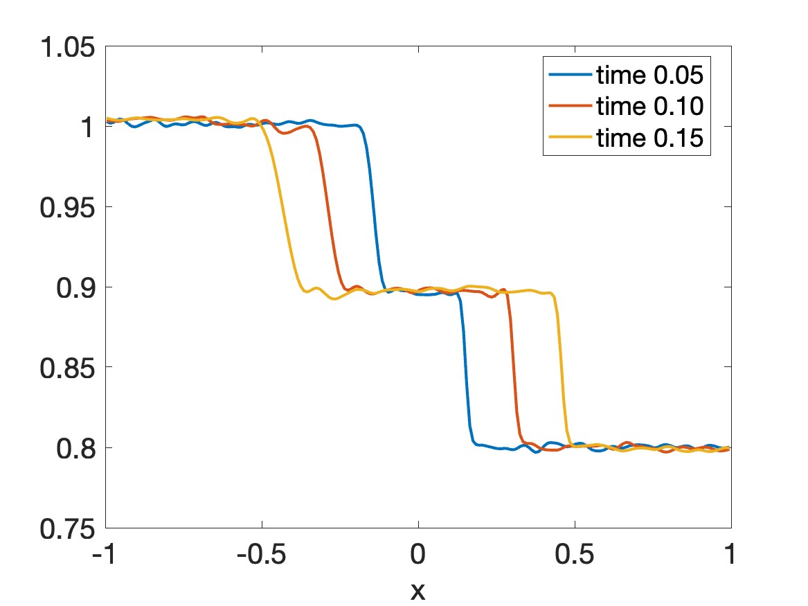
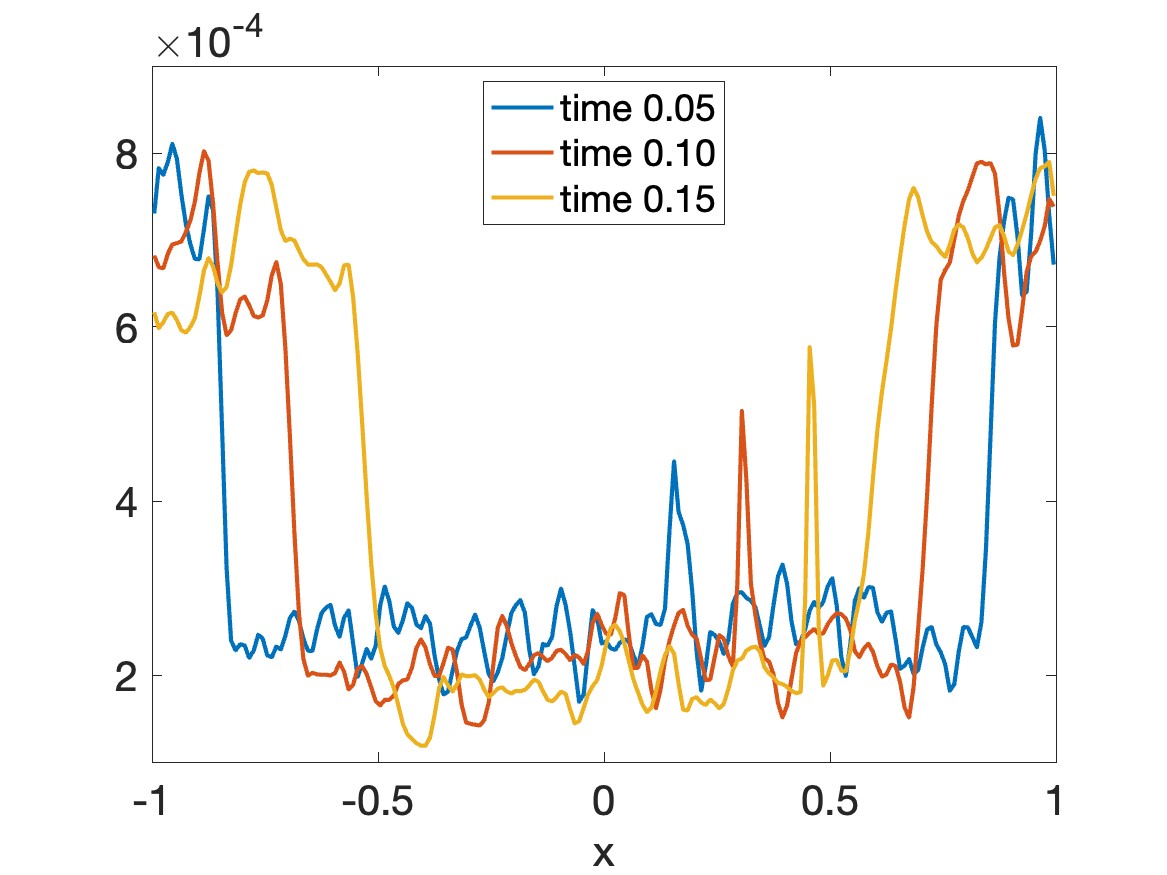
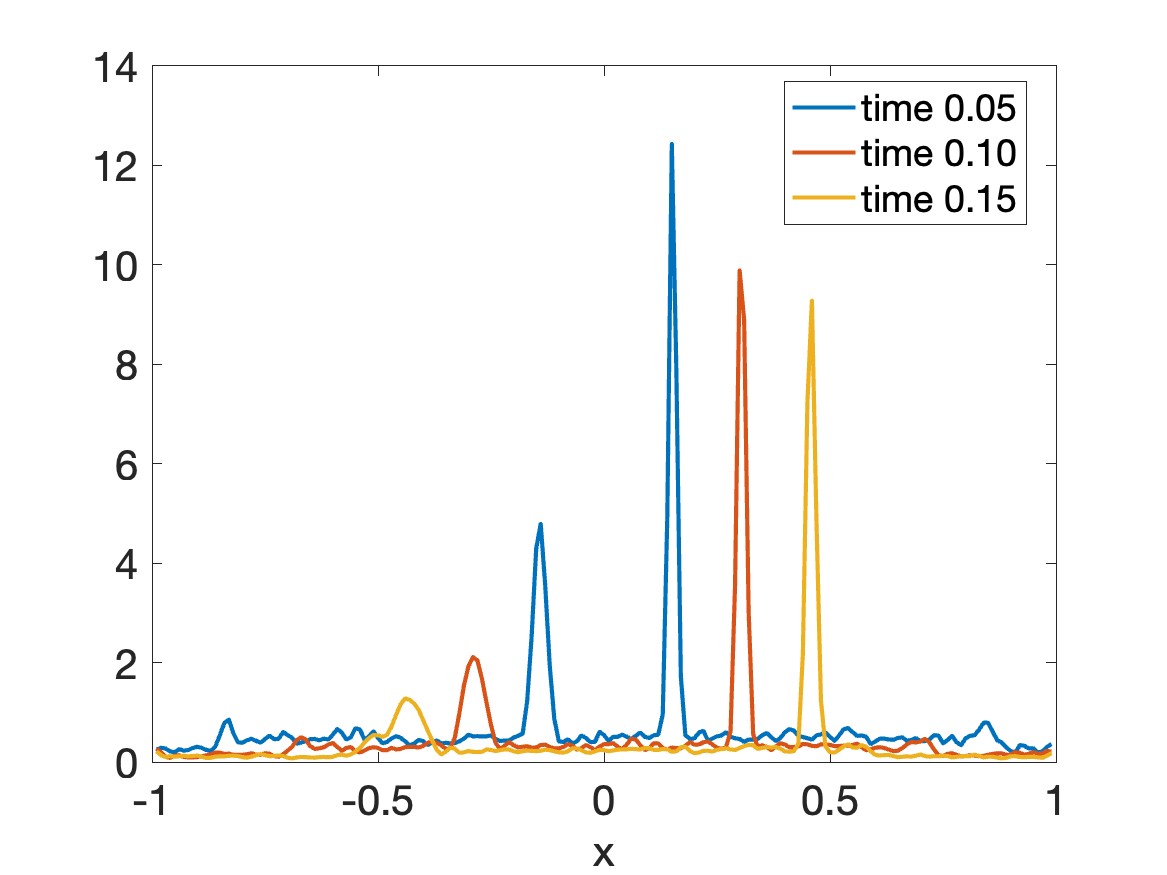
Figure 1: The mean solution of $h(x,t)$, $t=0.05,0.10,0.15$ in (4.1) using WENO with $\Delta x=10^{-2}$ and $\Delta t=10^{-5}$ for $K=100$ perturbed initial conditions (left). The corresponding variance (middle) and gradient second moment (right).

Remark 3.1.

We note that some variational data assimilation methods also incorporate structural information into the prior. For example, the objective function in 4DVar can be reformulated as an $\ell_{2}$ regularization [22]. Sharp features in the solution can be effectively recovered using $\ell_{1}$ regularization in the analysis step, [15]. In cases where the sparsity occurs in the gradient domain, the variational approach appropriately uses $\ell_{1}$ regularization for gradient of the state variable, [11, 14]. The mixed $\ell_{1}$-$\ell_{2}$ regularization framework has also been adopted in the method described in [16, 6]. In this case an extra term is added to the standard $\ell_{2}$ objective function in order to constrain the $\ell_{1}$ norm of the gradient of the analysis vector. Because variational data assimilation uses a global model/data fidelity balance parameter, none of these mentioned methods incorporate local information into the prior belief. By contrast, in our approach using the filtering problem for statistical data assimilation, we directly incorporate local structural information into the weighting matrix design. Moreover, since our approach uses $\ell_{2}$ minimization, there is a closed-form solution.

3.1 Designing the weighting matrix for densely sampled observations

In the ideal environment, where we have a densely sampled spatial observations, the observation operator $H$ in (3.1) is simply the identity matrix $I$. The most straightforward way to construct $W$ is then to use the (inflated and localized) ETKF covariance stemming from (2.23) and (2.24). We can reasonably choose $\mathcal{T}=I$ in (2.24), leading to a diagonal weighting matrix (thereby increasing computational efficiency) given by

$$W=\alpha^{2}\widehat{C}^{D},$$ (3.2)

where

$$\widehat{C}^{D}=\begin{pmatrix}\widehat{C}_{1}&0&\cdots&0\\ 0&\widehat{C}_{2}&\cdots&0\\ \vdots&\vdots&\ddots&\vdots\\ 0&0&\cdots&\widehat{C}_{n}\end{pmatrix},$$

with

$$\widehat{C}_{i}=\frac{1}{K-1}\sum_{k=1}^{K}(\widehat{v}_{i}^{(k)}-\widehat{m}_{i})^{2},\quad i=1,\cdots,n$$ (3.3)

being the sample variance of the state variable at each location derived from (2.15). Here $\widehat{v}_{i}^{(k)}=\widehat{{\mathbf{v}}}^{(k)}(x_{i})$ and $\widehat{m}_{i}=\widehat{{\mathbf{m}}}(x_{i})$, with the subscript denoting the location index. In some sense, using (3.2) to define $W$ could be viewed as a way to incorporate spatial information into posterior update. In particular, such information includes how well the prior mean approximates the ensembles at each grid point. This construction does not, however, separately take into account when the underlying solution admits a discontinuity. To this end it is well understood in other applications (e.g. TV regularization for image recovery) that incorporating such information into the prior typically improves the quality of the numerical solution. Moreover, as was discussed in Section 1, joint information from multiple observations (MMVs) can be used to determine how much to spatially vary the weight of the regularization term in the corresponding objective function. Drawing an analogy between the weighted $\ell_{1}$ joint sparsity image recovery algorithm in [1, 19], and the objective function in (3.1), where the ensemble corresponds to the MMVs in the image recovery problem, we are inspired to construct $W$ using joint information from the ensemble data so that the optimized solution is one that is able to distinguish discontinuous from smooth regions. Specifically we will use information from the spatial gradient of the state variable, which is sparse for a piecewise constant solution profile, and is therefore better suited for designing $W$ than the state variable. We now provide details for this construction.

In our problem we consider the grid to be uniform with mesh size $\Delta x$. For simplicity we compute the gradient using first order finite differencing,

$$d\widehat{v}^{(k)}_{i+\frac{1}{2}}=\frac{\widehat{v}^{(k)}_{i+1}-\widehat{v}^{(k)}_{i}}{\Delta x},$$ (3.4)

and note that neither the uniformity of the grid nor the approximation of the gradient are intrinsic to our approach. The second moment of the gradient at each cell center is then

$$\widehat{S}_{i+\frac{1}{2}}=\frac{1}{K}\sum_{k=1}^{K}\left(d\widehat{v}^{(k)}_{i+\frac{1}{2}}\right)^{2}.$$ (3.5)

We use (3.5) to approximate the second moment of the gradient at each grid point $\{x_{i}\}_{i=1}^{n}$ as

$$\widehat{S}_{i}=\begin{cases}\displaystyle\frac{1}{2}\widehat{S}_{\frac{3}{2}},\qquad i=1,\\[8.61108pt] \displaystyle\frac{1}{2}(\widehat{S}_{i-\frac{1}{2}}+\widehat{S}_{i+\frac{1}{2}}),\qquad i=2,\cdots,n-1\\[8.61108pt] \displaystyle\frac{1}{2}\widehat{S}_{n-\frac{1}{2}},\qquad i=n,\end{cases}$$ (3.6)

from which we construct the weighting matrix

$$W=\beta\widehat{S}^{D},\quad\beta>0,$$ (3.7)

with

$$\widehat{S}^{D}=\begin{pmatrix}\widehat{S}_{1}&0&\cdots&0\\ 0&\widehat{S}_{2}&\cdots&0\\ \vdots&\vdots&\ddots&\vdots\\ 0&0&\cdots&\widehat{S}_{n}\end{pmatrix}.$$

While the parameter $\beta$ plays a similar role to the inflation coefficient $\alpha$ in (3.2), due to the differences in $\widehat{S}^{D}$ and $\widehat{C}^{D}$, it does not have a lower bound of $1$.

3.2 Designing the weighting matrix for sparsely sampled observations

The diagonal weighting matrix $W$ is suitable when observations are densely sampled. We now seek a more flexible design for $W$ that could be adapted to accommodate a sparse observation environment. Based on $\widehat{C}_{i}$ in (3.3), the full covariance matrix $\widehat{C}$ has entries

$$\widehat{C}_{i,i^{\prime}}=\sqrt{\widehat{C}_{i}}\,r_{i,i^{\prime}}\sqrt{\widehat{C}_{i^{\prime}}},\quad i,i^{\prime}=1,\dots,n,$$ (3.8)

where $r_{i,i^{\prime}}$ given by

$$r_{i,i^{\prime}}=\frac{\displaystyle\frac{1}{K-1}\sum_{k=1}^{K}(\widehat{v}_{i}^{(k)}-\widehat{m}_{i})(\widehat{v}_{i^{\prime}}^{(k)}-\widehat{m}_{i^{\prime}})}{\displaystyle\sqrt{\frac{1}{K-1}\sum_{k=1}^{K}(\widehat{v}_{i}^{(k)}-\widehat{m}_{i})^{2}}\sqrt{\frac{1}{K-1}\sum_{k=1}^{K}(\widehat{v}_{i^{\prime}}^{(k)}-\widehat{m}_{i^{\prime}})^{2}}},$$ (3.9)

are the components of the correlation coefficient matrix $\widehat{R}$. The idea is then to generalize (3.7) by making use of the fact that the full covariance matrix $\widehat{C}$ in (3.8) is related to the variance through $\widehat{R}$. In this regard, we observe that $\widehat{C}$ in (3.8), which is equivalent to (2.15), can be constructed from its variance components given in (3.3). Based on the comparison of (3.2) to (3.7), we are similarly motivated to now construct a full gradient second moment matrix that incorporates the gradient second moment components given in (3.6) with the correlation coefficients in (3.9). That is, we directly substitute $\widehat{S}_{i}$ for $\widehat{C}_{i}$ in (3.8) to obtain $\widehat{S}$

$$\widehat{S}_{i,i^{\prime}}=\sqrt{\widehat{S}_{i}}\,r_{i,i^{\prime}}\sqrt{\widehat{S}_{i^{\prime}}}.$$ (3.10)

As before, we construct the weighting matrix as

$$W=\beta\widehat{S}\odot\mathcal{T},$$ (3.11)

with $\beta>0$ and $\mathcal{T}$ the user prescribed binary Toeplitz localization matrix as is used in (2.24).

Remark 3.2.

Based on the observation that (2.21) is equivalent to (3.8) for $\widehat{X}=(\widehat{C}^{D})^{\frac{1}{2}}\widetilde{X}$ when $\widetilde{X}$ is given by $\widehat{R}=\widetilde{X}\widetilde{X}^{T}$, rather than using (3.10) in the numerical implementation, we simply compute $\widehat{S}=\left((\widehat{S}^{D})^{\frac{1}{2}}\widetilde{X}\right)\left((\widehat{S}^{D})^{\frac{1}{2}}\widetilde{X}\right)^{T}$.

3.3 Structural refinement by clustering

Intuitively speaking, three types of information can be used to update the state variable at any particular location: (1) the observation data at that location; (2) the prior information at that location; and (3) relevant information coming from other (neighboring) locations. As discussed in Section 3.1, we can effectively rebalance these first two types of information using the gradient information via (3.7), while incorporating neighborhood information was described in Section 3.2 through (3.10). Utilizing such correlating information becomes increasingly important in cases where we lack observation data at that particular location. Moreover, when the underlying state variable has a discontinuity profile, gradient information provides a more appropriate model/data compromise, and in particular promotes solutions that “trust” prior information more. Intrinsically, then, there is an underlying assumption that the prediction method used to simulate the dynamic model is well-suited to solve PDEs that contain discontinuities in their solutions. We will return to this discussion in Section 4.1.

It is also possible to update the correlation matrix with the entries given by (3.9) which helps to refine the local information regarding discontinuities. In particular, the state variable at locations on either side of a discontinuity should be less correlated. We now propose a clustering approach to extract this information and improve our correlation update.

We begin by determining the jump discontinuity locations, which can be obtained using gradient information of the prior mean in (2.14) as

$$d\widehat{m}_{i+\frac{1}{2}}=\frac{\widehat{m}_{i+1}-\widehat{m}_{i}}{\Delta x}.$$ (3.12)

The set of discontinuity points are then chosen as the local extrema of (3.12). While there are several ways to do this, some assumptions regarding both the underlying problem and the available data are required. For example, one could impose constraints with respect to how close two shocks are able to occur. For ease of presentation here we assume that there is only one true discontinuity (which is consistent with our numerical example in Section 4) so that we are only looking for the global extrema in (3.12), which we define as

$$\xi=\underset{i}{\text{argmax}}\{|d\widehat{m}_{i+\frac{1}{2}}|\}$$ (3.13)

We emphasize that neither the number of discontinuities nor the way we determine their locations inherently limits the use of our method, which can indeed consider an unknown number of discontinuities along with more sophisticated (e.g. higher order) ways of determining their locations. Finally, we note that we choose to use (3.12) rather than (3.4), which is more likely affected by noise.

Once $\xi$ in (3.13) is determined, we can define the discontinuity region

$$R^{D}=\{i:|i-\xi|\leq dist\}$$ (3.14)

where $dist\in\mathbb{Z}^{+}$ is predetermined to take into account both gradient steepness and the resolution of the grid. The domain is then decomposed into the discontinuity region and two smooth regions

$$R^{S}_{1}=\{i:i<i^{\prime}\quad\forall i^{\prime}\in R^{D}\}\qquad\text{and}\qquad R^{S}_{2}=\{i:i>i^{\prime}\quad\forall i^{\prime}\in R^{D}\}.$$

The entries of the correlation coefficient matrix in (3.9), are modified according to each entry’s proximity to a discontinuity region as

$$\widetilde{r}_{i,i^{\prime}}=\begin{cases}r_{i,i^{\prime}}\quad\text{if }i=i^{\prime}\text{ or }i,i^{\prime}\in R^{S}_{\kappa},\,\kappa=1,2,\\ 0\quad\text{ otherwise },\\ \end{cases}$$ (3.15)

leading to the modified correlation coefficient matrix $\widetilde{R}$. By construction, (3.15) imposes local information so that only grid points occurring in the same smooth region can be correlated. That is, points on opposite sides of a discontinuity region will not be correlated, and moreover the solution within a discontinuous region will not utilize information from neighboring locations. Replacing the correlation coefficients in (3.10) with (3.15) we obtain the block diagonal matrix (thereby also improving computational efficiency)

$$\widetilde{S}_{i,i^{\prime}}=\sqrt{\widehat{S}_{i}}\,\widetilde{r}_{i,i^{\prime}}\sqrt{\widehat{S}_{i^{\prime}}},$$ (3.16)

from which we compute

$$W=\beta\widetilde{S}\odot\mathcal{T},$$ (3.17)

as in (3.11) for some parameter $\beta$ and localization matrix $\mathcal{T}$.

3.4 Numerical implementation

Using the results from each previous section, we now recap the modified ETKF method using the new second moment weighting matrix, $W=\beta\widetilde{S}\odot\mathcal{T}$, where $\widetilde{S}$ is given by (3.16). (We use $\widetilde{S}=\widehat{S}$ in (3.10) when clustering is not included.) We note again that both parameter $\beta>0$ localization matrix $\mathcal{T}$ are user prescribed. Here we choose $\mathcal{T}=I$ when observations are densely sampled (Section 3.1) and to be tridiagonal with nonzero entries of $1$ when the observations are sparse (Section 3.2). At time $t_{j}$, the prior ensembles $\widehat{{\mathbf{v}}}^{(k)}$ are obtained through the dynamic model (2.2). The sample prior mean is computed using (2.14). The covariance matrix

$$\widehat{C}=\widehat{X}\widehat{X}^{T},$$

is generated using the non-inflated centered ensemble

$$\widehat{X}=\frac{1}{\sqrt{K-1}}\left[\widehat{{\mathbf{v}}}^{(1)}-\widehat{{\mathbf{m}}},\cdots,\widehat{{\mathbf{v}}}^{(K)}-\widehat{{\mathbf{m}}}\right].$$ (3.18)

We then construct $T$ and $X$ according to (2.20) and (2.19), and subsequently $\widetilde{S}$ as (3.16). To determine the posterior mean in the analysis step, we now solve

$${\mathbf{m}}=\underset{{\mathbf{v}}}{\text{arg min}}\ \mathbf{I}_{\text{filter}}({\mathbf{v}}).$$ (3.19a)

$$\mathbf{I}_{\text{filter}}({\mathbf{v}})=\frac{1}{2}|{\mathbf{y}}-H{\mathbf{v}}|_{\Gamma}^{2}+\frac{1}{2}|{\mathbf{v}}-\widehat{{\mathbf{m}}}|_{\beta\widetilde{S}\odot\mathcal{T}}^{2},$$ (3.19b)

This is followed by updates on the ensembles according to the transformation

$${\mathbf{v}}^{(k)}={\mathbf{m}}+{\bm{\zeta}}^{(k)},$$ (3.20)

where ${\bm{\zeta}}^{(k)}$ is defined by (2.22). We note that (3.19) can be analytically solved for ${\mathbf{m}}$ as

$$\left(H^{T}\Gamma^{-1}H+\left(\beta\widetilde{S}\odot\mathcal{T}\right)^{-1}\right){\mathbf{m}}=H^{T}\Gamma^{-1}{\mathbf{y}}+\left(\beta\widetilde{S}\odot\mathcal{T}\right)^{-1}\widehat{{\mathbf{m}}}.$$

Alternatively, to avoid direct computation of $(\beta\widetilde{S}\odot\mathcal{T})^{-1}$ we use the equivalent Sherman-Morrison-Woodbury formula yielding

$${\mathbf{m}}=(I-KH)\widehat{{\mathbf{m}}}+K{\mathbf{y}},$$ (3.21)

$$K=\beta\widetilde{S}\odot\mathcal{T}H^{T}S^{-1},\quad S=H\left(\beta\widetilde{S}\odot\mathcal{T}\right)H^{T}+\Gamma.$$ (3.22)

Algorithm 2 describes the modified ETKF framework using the new weighting matrix with localization and clustering techniques.

Algorithm 2 modified ETKF method with localization and clustering techniques

Initialize ensembles ${\mathbf{v}}^{(k)}_{0}$, $k=1,\dots,K$. Choose parameter $\beta$ and localization matrix $\mathcal{T}$ for $W$ in (3.17).

for $j=1$ to $J-1$ do

     Compute prior ensembles $\displaystyle\widehat{{\mathbf{v}}}^{(k)}_{j+1}={\bm{\Psi}}({\mathbf{v}}^{(k)}_{j})$ for $k=1,\cdots,K.$

     if data observations are available at time instance $j+1$ then

         Compute prior mean $\displaystyle\widehat{{\mathbf{m}}}_{j+1}=\frac{1}{K}\sum_{k=1}^{K}\,\widehat{{\mathbf{v}}}^{(k)}_{j+1}$.

         Compute non-inflated centered ensemble $\displaystyle\widehat{X}_{j+1}=\frac{1}{\sqrt{K-1}}\left[\widehat{{\mathbf{v}}}^{(1)}_{j+1}-\widehat{{\mathbf{m}}}_{j+1},\cdots,\widehat{{\mathbf{v}}}^{(K)}_{j+1}-\widehat{{\mathbf{m}}}_{j+1}\right]$ and covariance matrix $\displaystyle\widehat{C}_{j+1}=\widehat{X}_{j+1}\,\widehat{X}_{j+1}^{T}$.

         Compute the transformation matrix $T_{j+1}$ and $X_{j+1}$ according to (2.20) and (2.19) respectively.

         Compute the full gradient second moment matrix $\widetilde{S}_{j+1}$ according to (3.16).

         Solve the minimization problem for the posterior mean ${\mathbf{m}}_{j+1}$ through

$${\mathbf{m}}_{j+1}=(I-KH)\widehat{{\mathbf{m}}}_{j+1}+K{\mathbf{y}}_{j+1},$$

$$K=\beta\widetilde{S}_{j+1}\odot\mathcal{T}H^{T}S^{-1},\quad S=H\left(\beta\widehat{S}_{j+1}\odot\mathcal{T}\right)H^{T}+\Gamma.$$

         Update the posterior ensembles according to the transformation (2.17) where ${\bm{\zeta}}^{(k)}_{j+1}$ is defined by (2.22).

     else $\displaystyle{\mathbf{v}}^{(k)}_{j+1}=\widehat{{\mathbf{v}}}^{(k)}_{j+1}$ for $k=1,\cdots,K.$

     end if

end for

Remark 3.3.

We note that in contrast to traditional ETKF, where inflation is directly applied to the centered ensembles via (2.23), here we use the non-inflated ensemble (3.18) to compute the covariance matrix which is in turn employed to construct the correlation coefficient matrix with entries given by (3.9). The tuning parameter $\beta$ in the resulting weighting matrix $W=\beta\widetilde{S}\odot\mathcal{T}$ plays a similar role to the inflation coefficient $\alpha$.

4 Numerical examples

We use the one-dimensional dam break problem governed by shallow water equations as our model problem to demonstrate the performance of our new method. The dam break problem yields a solution that has both shock and contact discontinuities, making it challenging for traditional statistical data assimilation techniques. By contrast, our approach is designed especially for this class of problems. Conveniently, the analytical solution provided in [36] allows us to conduct some error analysis. For simplicity this investigation only considers the 1D case. Our method is not inherently limited, however, and 2D problems will be discussed in future work.

4.1 1D dam break problem

Assuming a flat bottom, the 1D shallow water equations in conservation form is given by

$$h_{t}+(hu)_{x}=0,$$ (4.1a)

$$(hu)_{t}+(hu^{2}+\frac{1}{2}gh^{2})_{x}=0,$$ (4.1b)

where $h=h(x,t)$ is the depth of the water, $u=u(x,t)$ is the (depth-averaged) fluid velocity, and $g=9.81$ is the acceleration due to gravity. Here $x$ is the location and $t$ is the time.

For the dam break problem, the fluid is initially at rest on both sides of a dam located at $x=0$. At time $t=0$ a dam break is simulated by suddenly removing the dam wall. Stoker [36] provides an analytical solution for the problem with initial conditions

$$h(x,0)=\begin{cases}h_{0},\quad x<0\\ h_{1},\quad x>0\end{cases}{\quad\hbox{and}\quad}u(x,0)=0.$$ (4.2)

The solution consists of a shock front propogating to the right and a rarefaction wave propagating to the left. This analytical solution will serve as our underlying truth for the test problems in Section 4.2 and Section 4.3 and will be referred to as the “Stoker solution”.

For the experiments conducted in Section 4.2 and Section 4.3 we let $h_{0}=1$, $h_{1}=0.8$, while Section 4.4 we consider oscillatory initial conditions. The spatial domain is always $[-1,1]$. To set up our experiments, we first numerically simulate the coupled system in (4.1) and then use the corresponding solution for the velocity $u(x,t)$ as the synthetic data for the data assimilation on recovering the water depth, $h(x,t)$.

It is well understood that for problems with solutions containing discontinuities, traditional higher-order finite difference schemes typically yield spurious oscillations near discontinuities, which may pollute smooth regions and even lead to instability, causing blowups of the schemes [33]. The WENO method [29] is designed to achieve higher-order accuracy in smooth regions while sharply resolving discontinuities in an essentially non-oscillatory fashion. Because of this, we choose to use WENO spatial discretization along with Lax-Friedrichs flux splitting. To close the system we apply homogeneous Dirichlet boundary conditions ($u=0$) at both ends of the domain, and use the total variation diminishing third-order Runge-Kutta (TVDRK3) time integration scheme [29] with a time step that satisfies the CFL condition. No attempt was made to optimize parameters with regard to either increased resolution or efficiency.

To simplify our presentation, our numerical experiments only uses (4.1a), the depth of the water $h$ advected by the transport equation, for the dynamic model (2.2). We assume that the fluid velocity $u(x,t)$ is known, with its value at any point in the domain taken from the numerical solution of the coupled problem. The domain $[-1,1]$ is uniformly discretized over $n=1001$ points, with $x_{i}=-1+(i-1)\Delta x$, $i=1,\dots,n$, yielding $\Delta x=\frac{2}{n-1}=2\times 10^{-3}$. We use $\Delta t=CFL\#\Delta x$ to integrate in time, with $CFL\#=0.1$ to ensure the CFL condition is satisfied (so that $\Delta t=2\times 10^{-4}$). The observation data is created from the Stoker solution with $\Gamma=\gamma^{2}I$, $\gamma=0.01$, and is observable every $\Delta t_{obs}=5\Delta t=10^{-3}$. We further consider two observational data environments: (1) The densely sampled case, where observations are made at every point in the spatial domain; and (2) the sparsely sampled case, where observations are available at every other point. Finally, the $K=100$ ensembles in Algorithm 2 are obtained from the data assimilation solution initialized from either (4.2) or (4.6), and in both cases containing additive i.i.d. noise with mean $0$ and standard deviation $0.1$.

Similar to the discussion surrounding Figure 1, we now show Figure 2 to demonstrate the benefits of using the gradient second moment of the prior ensembles to generate the weighting matrix in Algorithm 2. Specifically, the figure shows the mean, variance and gradient second moment of the prior ensembles for the densely sampled observation case described in Section 3.1 at time instances $0.05$, $0.10$ and $0.15$, where the prior ensembles are obtained via Algorithm 2. Once again we see that although the solution clearly exhibits discontinuities at each time instance, the variance is not able to delineate any local structural information. By contrast, the gradient second moment not only extracts each discontinuity location, but also apparently distinguishes between shocks and steep gradients, suggesting its potential benefits on the model/data compromise. More details will follow in Sections 4.2 and 4.3.

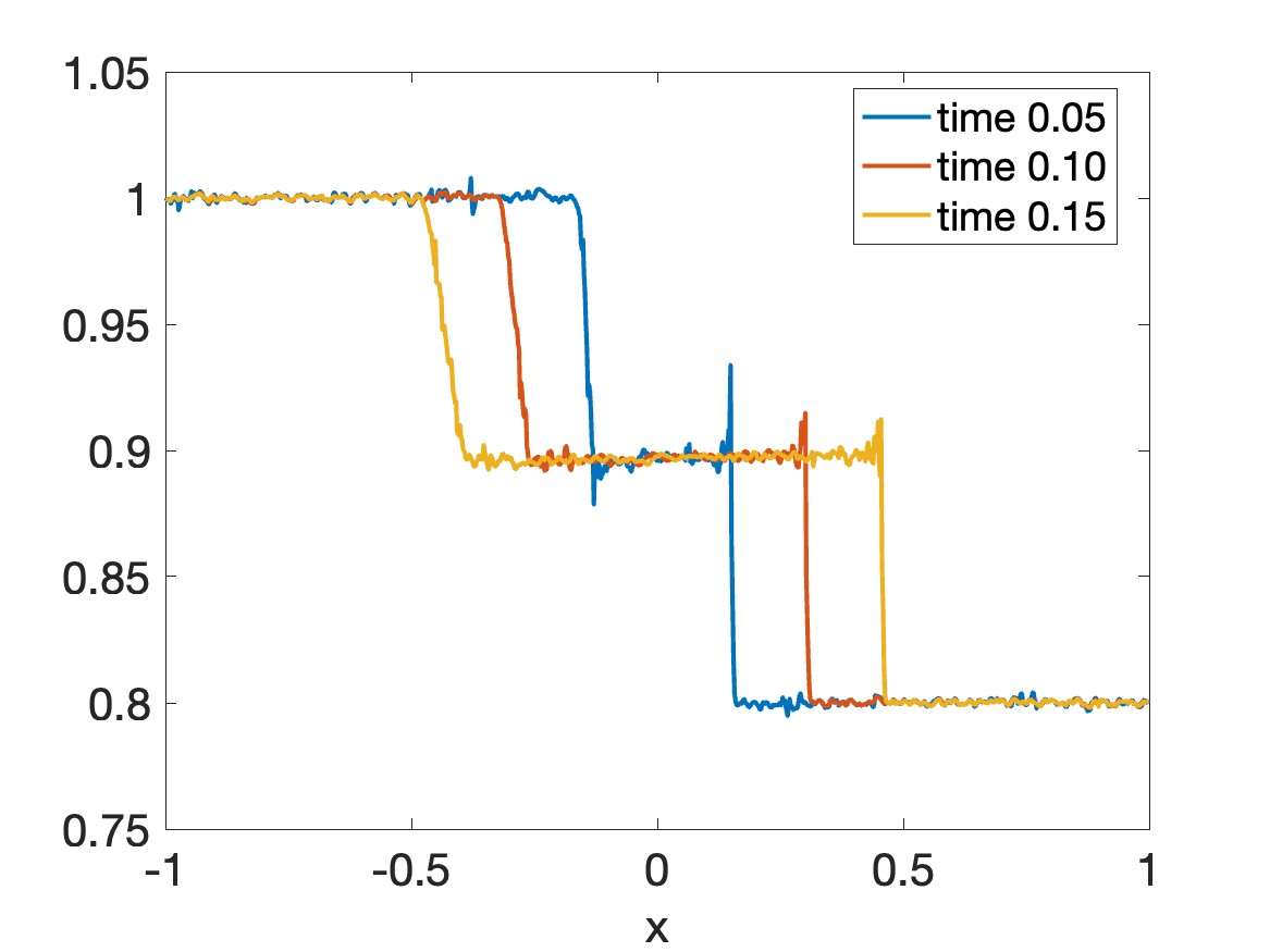
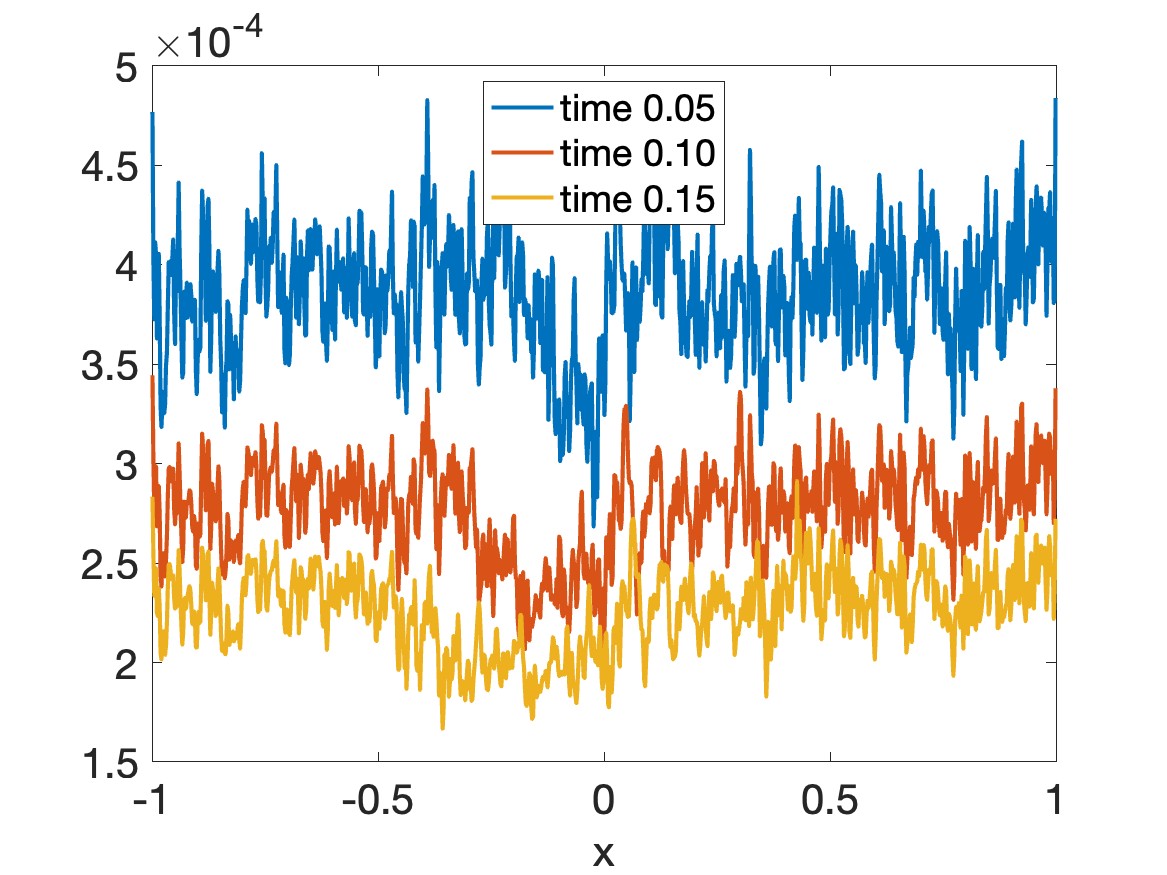
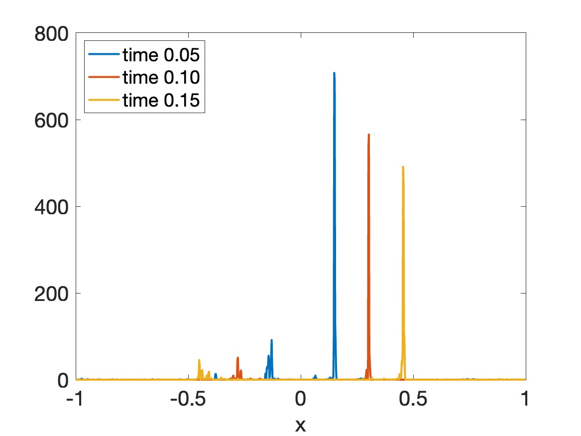
Figure 2: The mean solution of the prior ensembles of $h(x,t)$, $t=0.05,0.10,0.15$ as determined by Algorithm 2. The corresponding variance (middle) and gradient second moment (right).

We will analyze our results by computing the pointwise square of the error as defined by

$$err(x_{i},t)=(h(x_{i},t)-h_{i}(t))^{2},\quad i=1,\dots,n,$$ (4.3)

where $h(x_{i},t)$ is the Stoker solution at time $T$ for each $x_{i}$ and $h_{i}(t)$ is the posterior mean solution obtained either from Algorithm 1 or Algorithm 2, along with the $\ell_{1}$ and $\ell_{2}$ errors respectively given by

$$e_{\ell_{1}}(t_{j})=\frac{\displaystyle\sum_{i=1}^{n}|h(x_{i},t_{j})-h_{i}(t_{j})|}{\displaystyle\sum_{i=1}^{n}|h(x_{i},t_{j})|}$$ (4.4)

and

$$e_{\ell_{2}}(t_{j})=\frac{\displaystyle\sqrt{\sum_{i=1}^{n}(h(x_{i},t_{j})-h_{i}(t_{j}))^{2}}}{\displaystyle\sqrt{\sum_{i=1}^{n}(h(x_{i},t_{j}))^{2}}}$$ (4.5)

for each $t_{j}=j\Delta t$, $j=1,\cdots,J$, with $\Delta t=\frac{T}{J}$.

4.2 Densely sampled observations

We now compare results obtained using Algorithm 2 with localization matrix $\mathcal{T}=I$ to those obtained via Algorithm 1 for the ideal densely sampled observation case. The inflation parameter $\alpha$ is handtuned to produce a “good” root mean square error (RMSE), and here we choose $\alpha=1.5$. To determine $\beta$ for the gradient second moment weighting matrix $W=\beta\widehat{S}^{D}$ (c.f. (3.7)), we follow the general principle that $\beta$ should be chosen so that $W$ has comparable magnitude to that of the prior covariance matrix used in Algorithm 1. In this regard we choose $\beta$ such that $\max_{i,i^{\prime}}(W_{i,i^{\prime}})=0.003$, $1\leq i,i^{\prime}\leq n$.

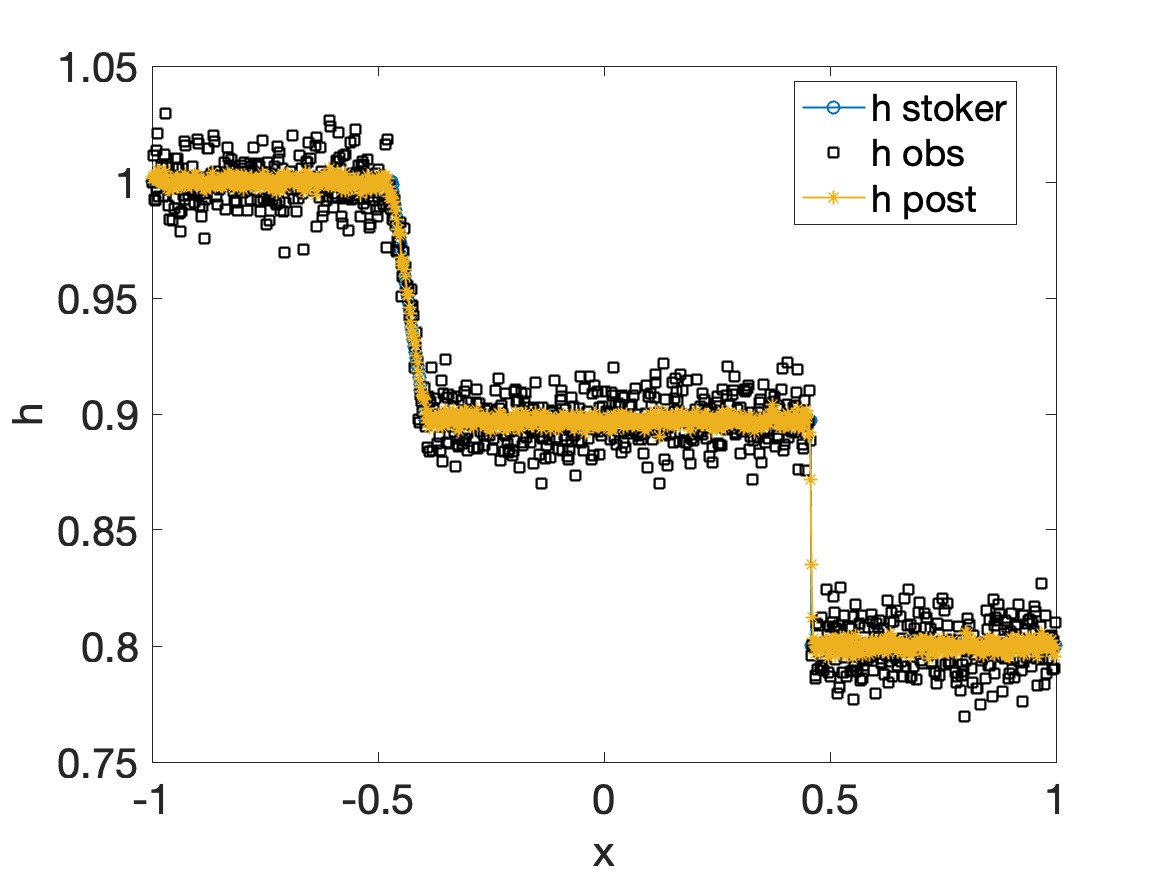
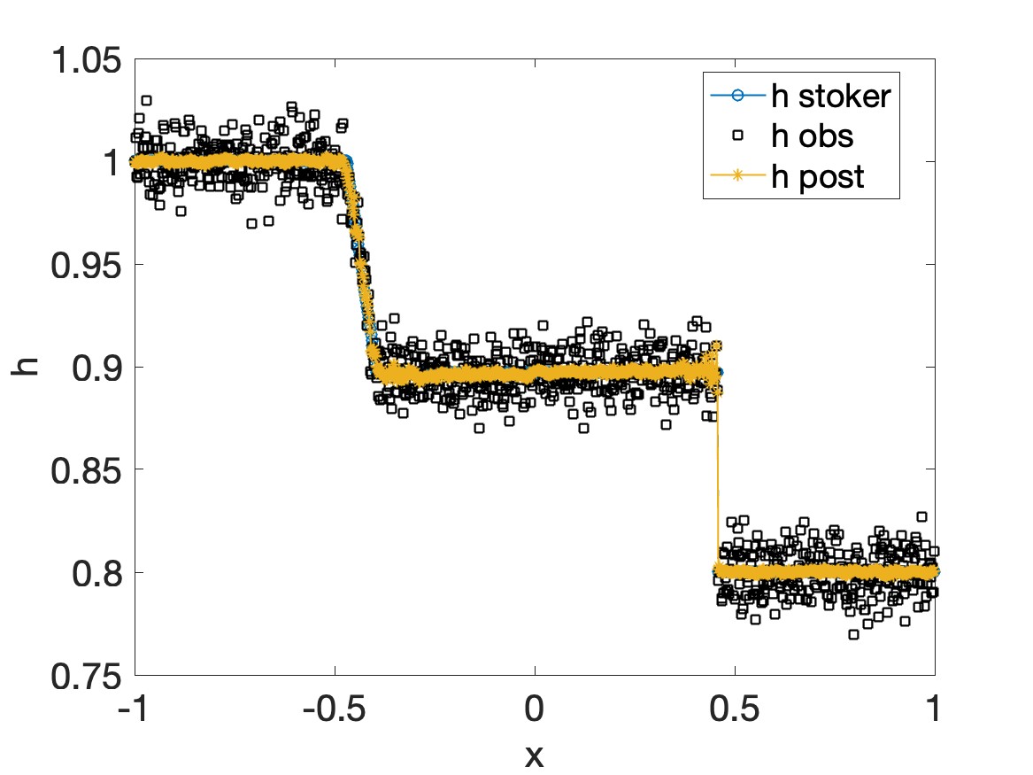
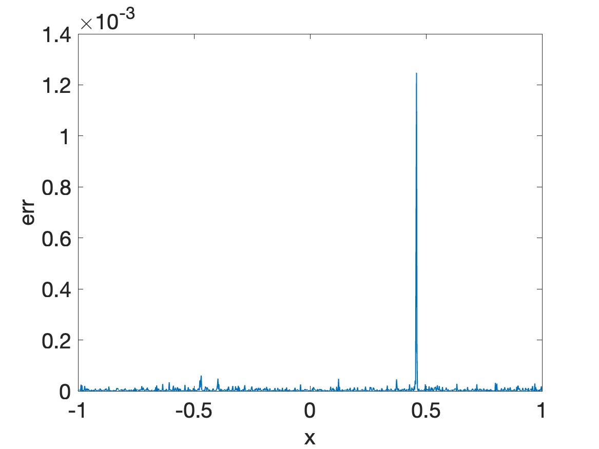
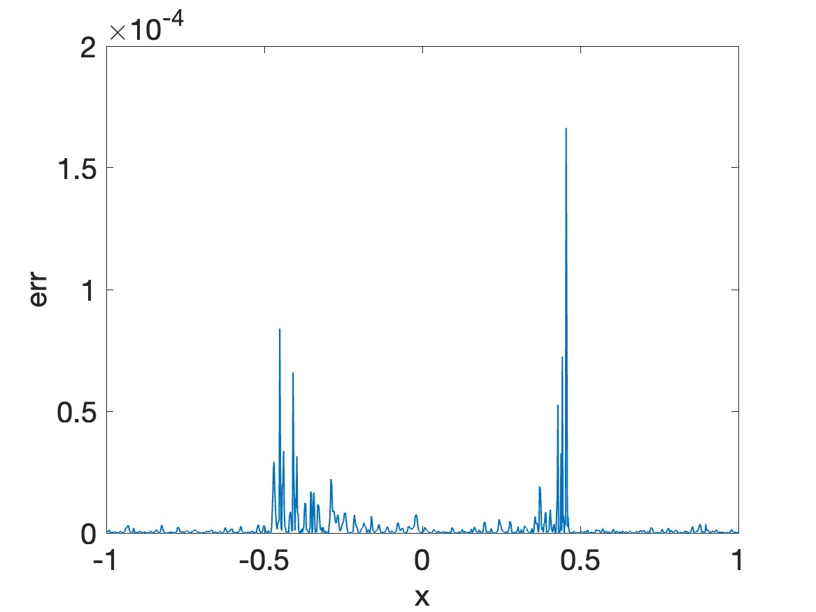
Figure 3: (top) Numerical solutions for the posterior mean of depth $h(x,0.15)$ as obtained by (left) Algorithm 1 and (right) Algorithm 2. (bottom) Corresponding pointwise posterior error defined by (4.3).

Figure 3 (top) shows the numerical solutions of depth $h(x,0.15)$, along with the Stoker solution and the observational data, as obtained by (left) Algorithm 1 and (right) Algorithm 2, each using the parameter values as already prescribed. Figure 3 (bottom) displays the corresponding pointwise squared posterior errors using (4.3). Observe that employing the gradient second moment weighting matrix not only provides a less oscillatory solution in the smooth regions, but it also generates a more highly resolved shock. Comparing the magnitudes of the error in Figure 3 (bottom) further verifies these observations.

Figure 4 displays the $\ell_{1}$ and $\ell_{2}$ errors given respectively by (4.4) and (4.5) obtained using both Algorithm 1 and Algorithm 2 in the time domain $[0.03,0.15]$. The first time interval is omitted since the solutions have not yet reached a stationary state. Once again we observe that Algorithm 2 yields smaller posterior error than Algorithm 1 does.

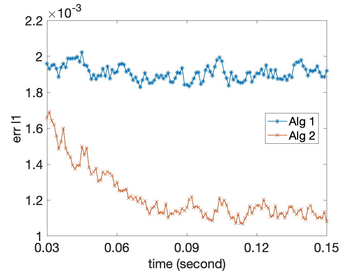
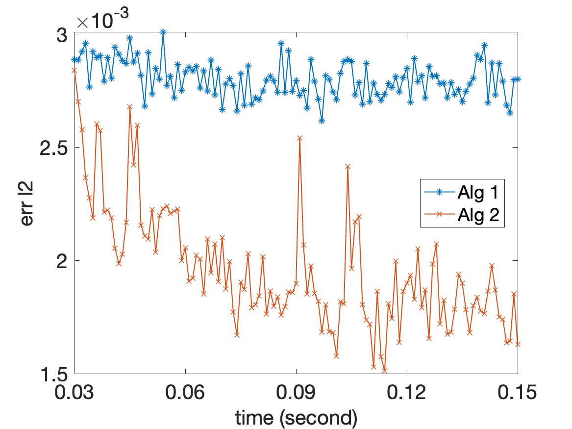
Figure 4: Comparison of the (left) $\ell_{1}$ error in (4.4) and (right) $\ell_{2}$ error in (4.5) produced by Algorithm 1 and Algorithm 2 in the time domain $[0.03,0.15]$.

4.3 Sparsely sampled observations

We now present results for the sparsely sampled observation case, that is, where data are observed at every other grid point in the spatial domain. In contrast to the densely sampled case, where we used $\mathcal{T}=I$ in the cosntruction of $W$, here the localization matrix $\mathcal{T}$ is tridiagonal with nonzero entries of $1$. We compare results obtained using (1) the localized covariance as described in Algorithm 1, (2) the localized gradient second moment without clustering, using Algorithm 2 with $W$ defined by (3.11), and (3) the localized gradient second moment with clustering, using Algorithm 2 with $W$ defined by (3.17). We correspondingly choose parameters $\alpha=1.3$ in Algorithm 1 and $\beta$ such that $\max_{i,i^{\prime}}(W_{i,i^{\prime}})=0.0027$, $1\leq i,i^{\prime}\leq n$ in Algorithm 2. We furthermore use $dist=1$ in (3.14) when employing clustering in Algorithm 2.

Figure 5 (top) shows the numerical solutions of depth $h(x,0.3)$, along with the Stoker solution and the observational data, as obtained by (left) Algorithm 1, (middle) Algorithm 2 with $W$ in (3.11) and (right) Algorithm 2 with $W$ in (3.17), each using the parameter values as already prescribed. Figure 3 (bottom) displays the corresponding pointwise squared posterior errors using (4.3). While employing the gradient second moment weighting matrix without clustering yields a less oscillatory solution in the smooth regions, incorporating clustering appears to help mitigate the overshoots at the shock location. These observations are verified when comparing the magnitudes of the error in Figure 5 (bottom).

Figure 6 (left) and Figure 6 (middle) display the $\ell_{1}$ and $\ell_{2}$ errors given respectively by (4.4) and (4.5) obtained using Algorithm 1, Algorithm 2 with $W$ in (3.11) and Algorithm 2 with $W$ in (3.17) for the time domain $[0.03,0.3]$. The first time interval is omitted since the solutions have not yet reached a stationary state. Figure 6 (right) shows the quadratic polynomial fit for the log of pointwise squared posterior errors at time $t=0.3$ in the smooth domain $[-0.5,0.5]$. The results are consistent with those shown in Figure 5.

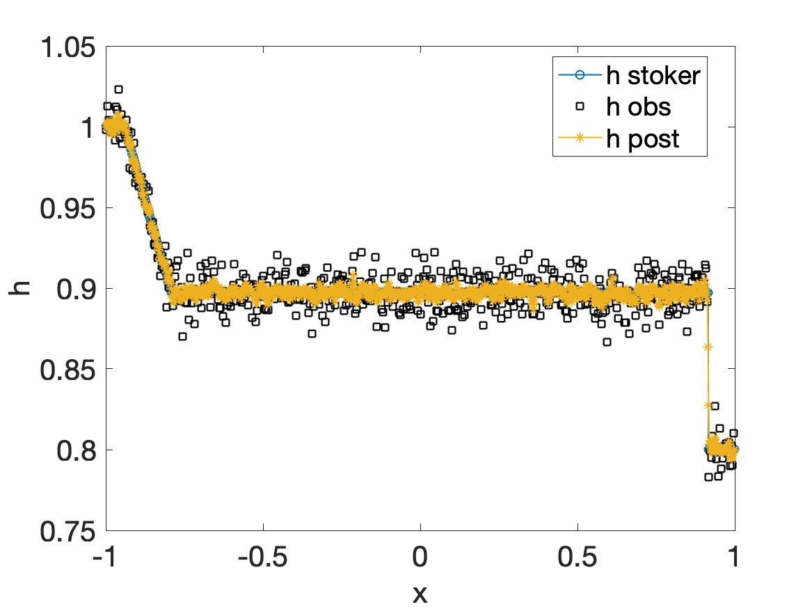
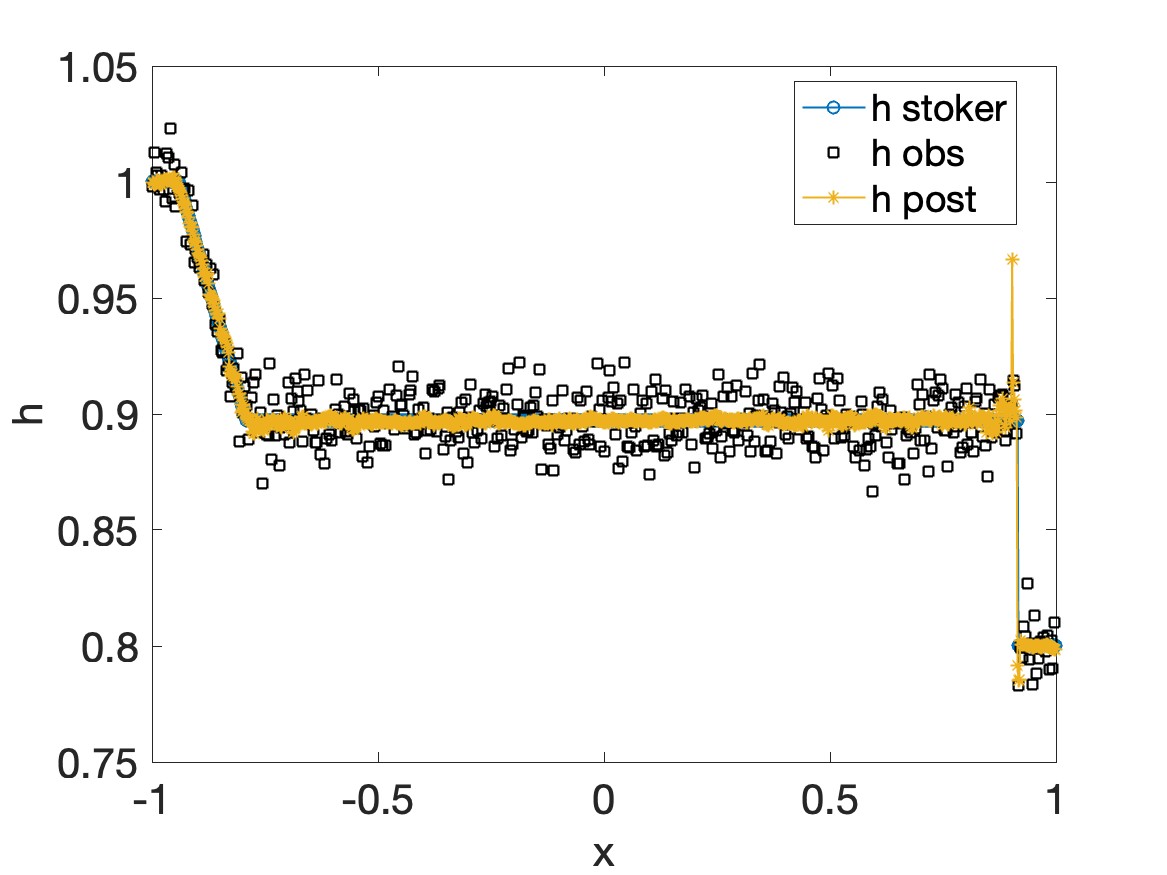
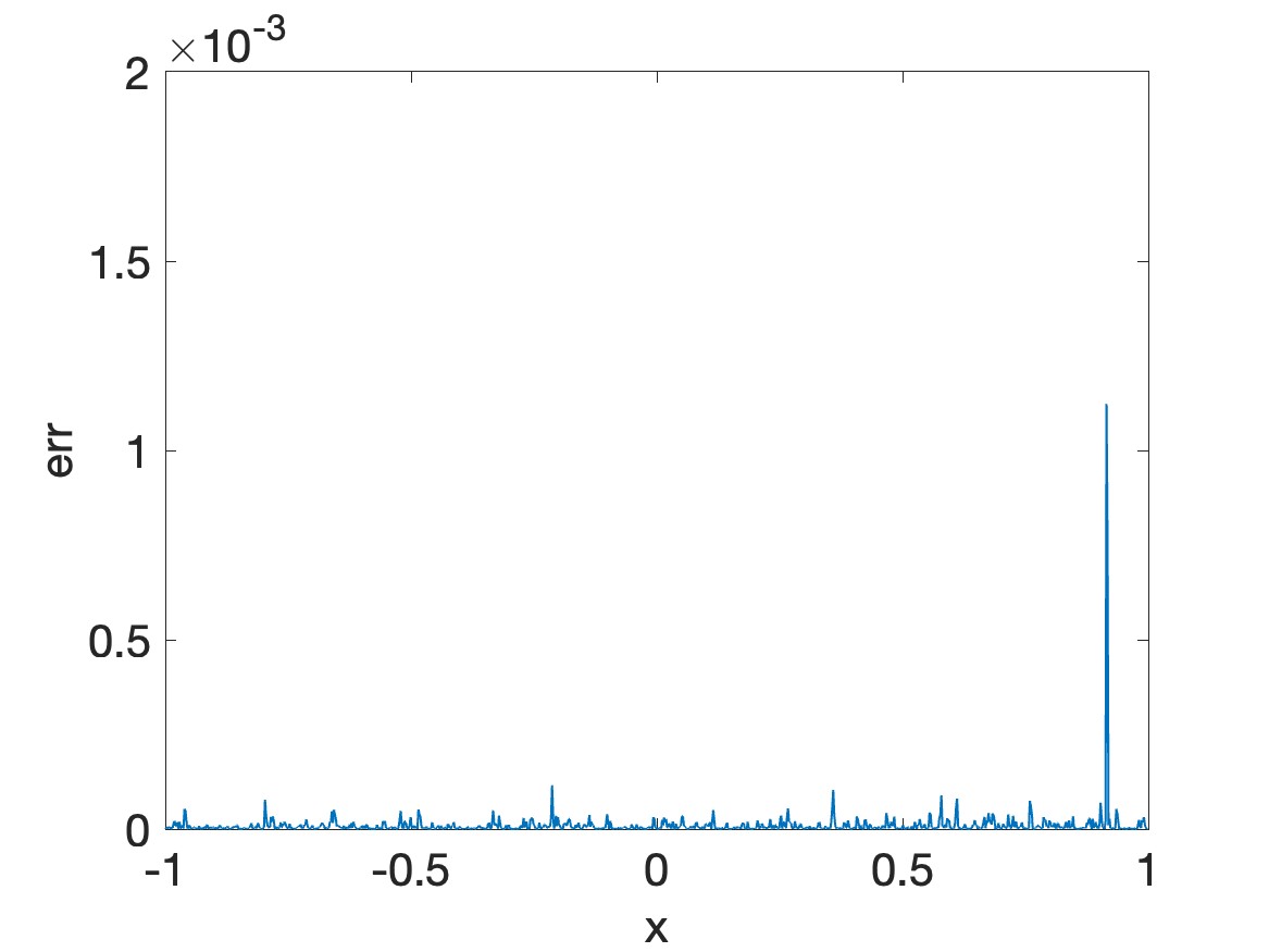
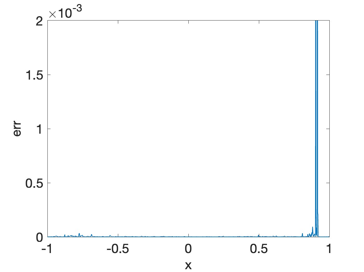
Figure 5: (top) Numerical solutions for the posterior mean of depth $h(x,0.3)$ as obtained by (left) Algorithm 1, (middle) Algorithm 2 without clustering and (right) Algorithm 2 with clustering. (bottom) Corresponding pointwise squared posterior error defined by (4.3).

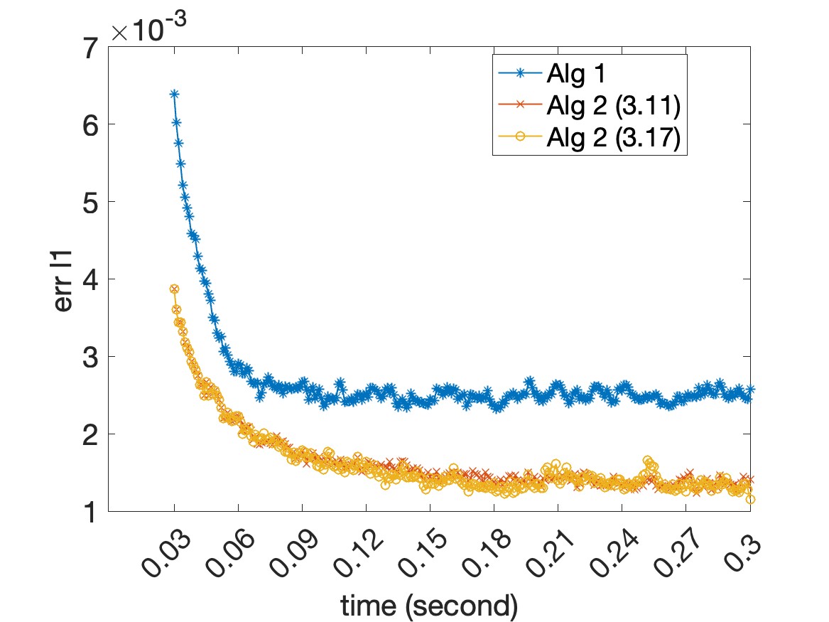
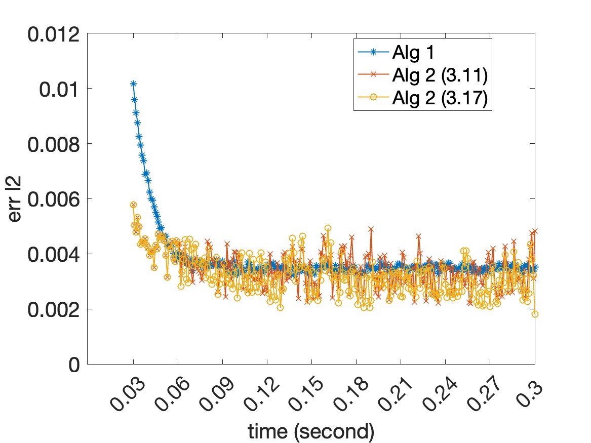
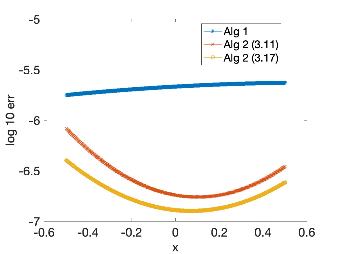
Figure 6: Comparison of Algorithm 1 and Algorithm 2, both with and without clustering. (Left) $\ell_{1}$ and (middle) $\ell_{2}$ errors in the time domain $[0.03,0.3]$, (right) quadratic polynomial fit for the log of pointwise squared posterior error of depth $h(x,0.3)$ in the spatial domain $[-0.5,0.5]$.

4.4 Shallow water equations with oscillatory behavior

As a final test we consider (4.1) with $u(x,0)=0$ and oscillating initial conditions for $h$ given by

$$h(x,0)=\begin{cases}1+0.03\sin(30x),\quad-1<x<-0.5,\\ 1,\quad-0.5<x<0,\\ 0.8,\quad 0<x<1.\end{cases}$$ (4.6)

These oscillations will remain in the solution for all simulation time, and present a greater challenge to data assimilation algorithms. Since there is no analytical solution, the true solution is approximated using WENO with more highly resolved spatial and temporal grids given by

$$\Delta x=1\times 10^{-4},\quad\Delta t=1\times 10^{-5}.$$

As in Section 4.3, we assume we are able to observe data at every other grid point (sparsely sampled observation case), and choose the same numerical parameters for our experiments. Once again we compare the results using Algorithm 1 with those using Algorithm 2 with and without clustering.

Figure 7 (top) compares the posterior mean of the depth $h(x,0.3)$ as obtained by Algorithm 1 and Algorithm 2 with and without clustering, while Figure 7 (bottom) compares their corresponding pointwise error defined by (4.3). Figure 8 shows the $\ell_{1}$ and $\ell_{2}$ errors for each of these approaches over time, together with the quadratic polynomial fit for the log pointwise error at time $t=0.3$ in the smooth region $[-0.5,0.5]$. It is evident that using Algorithm 2 yields more accurate results, and that clustering further helps to reduce the overshoots in the discontinuity regions.

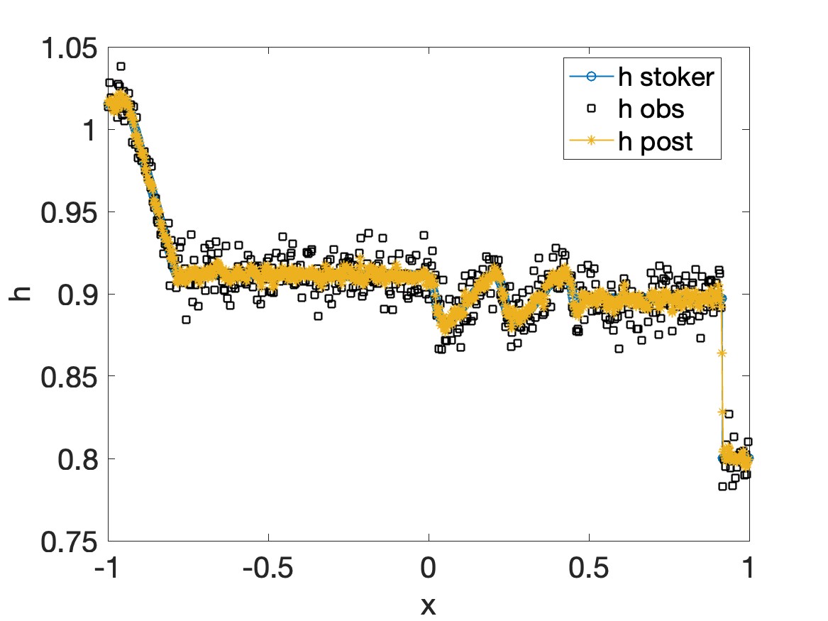
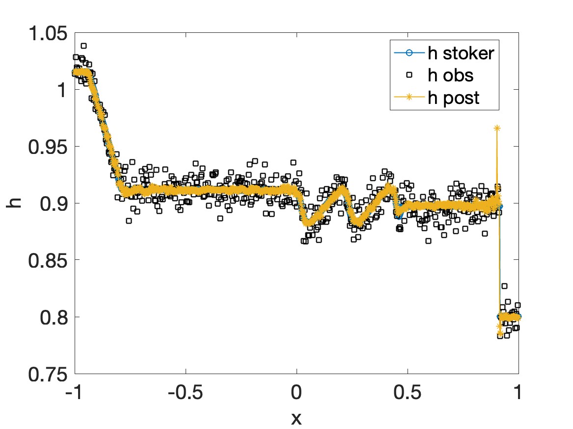
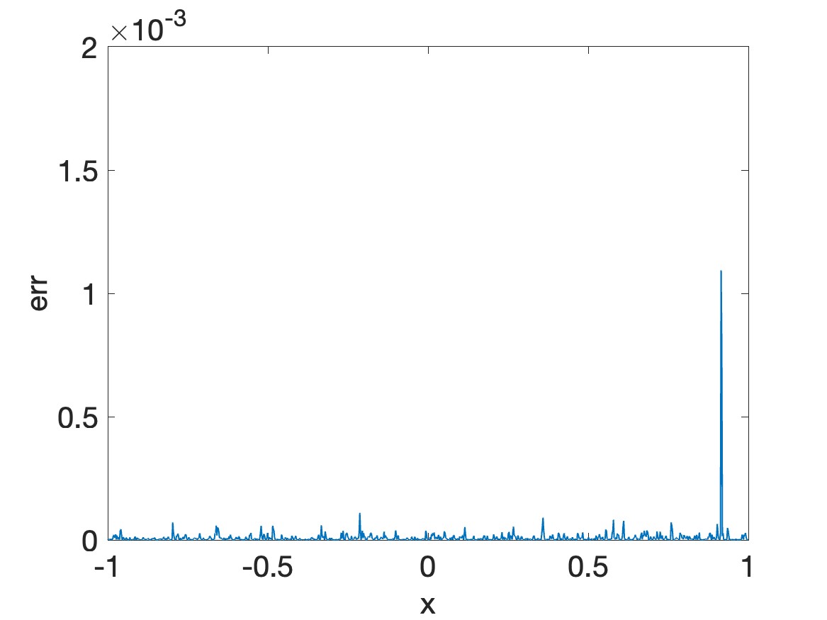
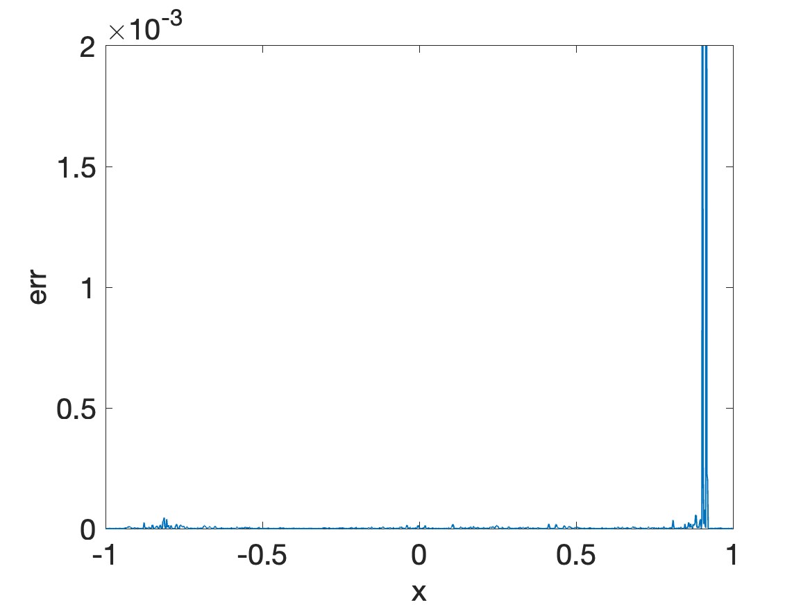
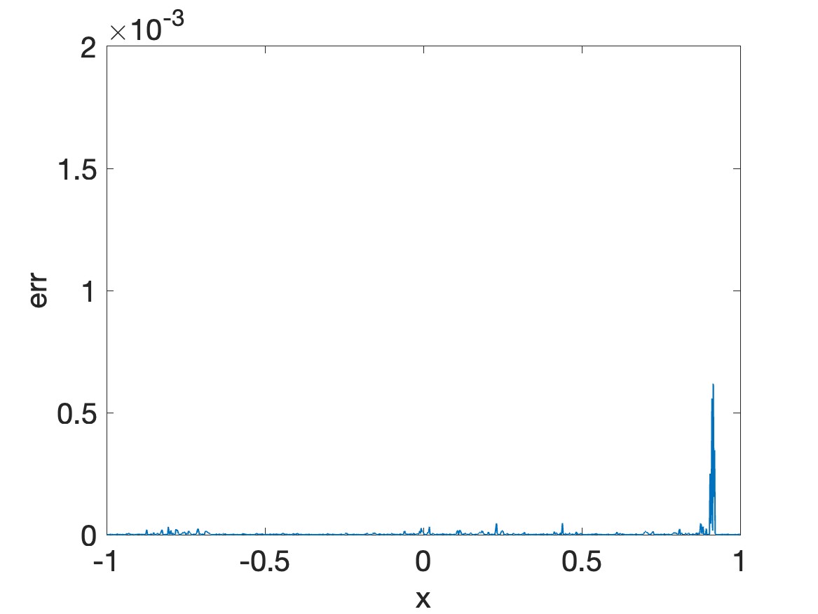
Figure 7: (top) Numerical solutions for the posterior mean of depth $h(x,0.3)$ as obtained by (left) Algorithm 1, (middle) Algorithm 2 without clustering and (right) Algorithm 2 with clustering. (bottom) Corresponding pointwise posterior error defined by (4.3).

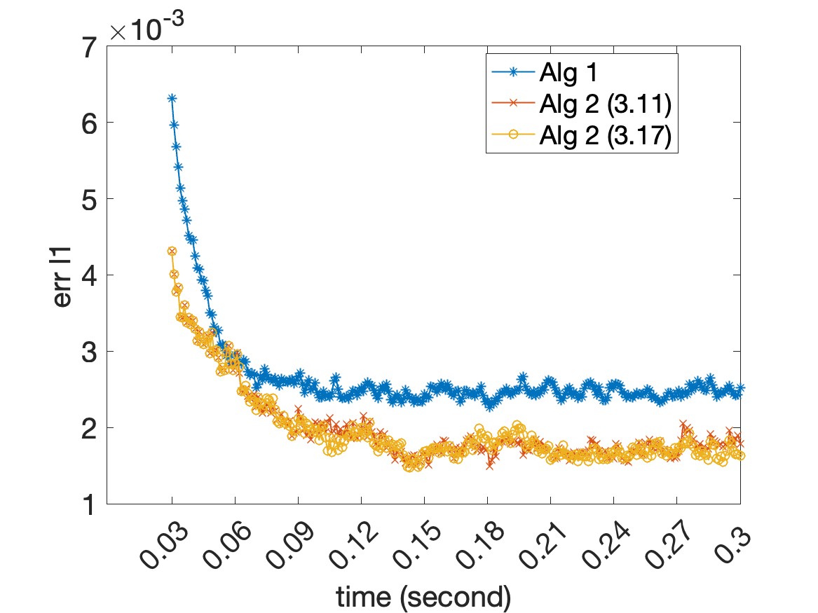
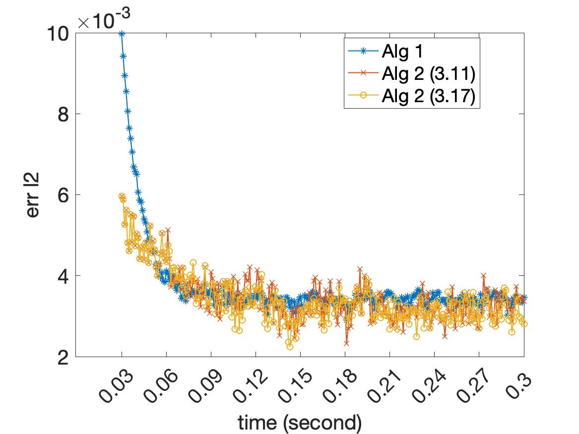
Figure 8: Comparison of Algorithm 1 and Algorithm 2, both with and without clustering. (Left) $\ell_{1}$ and (middle) $\ell_{2}$ errors in the time domain $[0.03,0.3]$, (right) quadratic polynomial fit for the log of pointwise squared posterior error of depth $h(x,0.3)$ in the spatial domain $[-0.5,0.5]$.

5 Concluding remarks

This investigation develops a new structurally informed non-Gaussian prior for the statistical data assimilation of non-linear PDEs that contain discontinuities in their solution profiles. Specifically, a new weighting matrix is constructed using second moment gradient information which then replaces the prior covariance matrix typically employed in ensemble-based Kalman filters. This prior reweights the model/data compromise. Our new approach furthermore includes using a numerical method in the prediction step that is able to capture shock information. Numerical experiments for both densely and sparsely sampled observations demonstrate that our new approach yields more accurate solutions when compared to ETKF, and can be enhanced further when neighborhood information surrounding the local discontinuity structure is also considered (clustering). Our method is robust and requires minimal hand-tuning of parameters. Finally, because the minimization is based on the $\ell_{2}$ norm, there is a closed-form solution so that no extra optimization algorithms are needed.

Our work presents a new paradigm for incorporating local discontinuity information into the prior design, and there are a number of ideas to explore in terms of both solving specific types of problems as well as practical implementation. For example, here we employed first order finite differencing used for computing the gradient. Higher order methods may be more appropriate if the underlying solution contains more variation or if the spatial grid is less resolved. In some cases this would allow a larger time step and make the prediction step more efficient. Other shock capturing techniques might also be beneficial in constructing the weighting matrix. For instance, the polynomial annihilation technique, [4, 5, 32], is a high order method that is able to detect both shock discontinuities and jumps in the gradient domain in multi-dimensions, and thus may improve the performance of the weighting matrix. Moreover, while $\ell_{2}$ minimization has the advantage of yielding a closed-form solution, $\ell_{1}$ regularization methods [9] are extensively used for sparse signal recovery and generally yield more sharply resolved structures. Finally, we note that other numerical methods, such as the discontinuous Galerkin (DG) or finite element method, may be more suitable for the prediction step for problems in higher dimensions on non-rectangular grids. Future work will compare these different approaches for use in our general framework.

References

- [1] B. Adcock, A. Gelb, G. Song, and Y. Sui. Joint sparse recovery based on variances. SIAM Journal on Scientific Computing, 41(1):A246–A268, 2019.
- [2] J. L. Anderson. An ensemble adjustment kalman filter for data assimilation. Monthly Weather Review, 129(12):2884 – 2903, 2001.
- [3] J. L. Anderson. An adaptive covariance inflation error correction algorithm for ensemble filters. Tellus A: Dynamic Meteorology and Oceanography, 59(2):210–224, 2007.
- [4] R. Archibald, A. Gelb, and J. Yoon. Polynomial fitting for edge detection in irregularly sampled signals and images. SIAM Journal on Numerical Analysis, 43(1):259–279, 2005.
- [5] R. Archibald, R. Saxena, A. Gelb, and D. Xiu. Discontinuity detection in multivariate space for stochastic simulations. Journal of Computational Physics, 228(7):2676–2689, 2009.
- [6] N. Asadi, K. A. Scott, and D. A. Clausi. Data fusion and data assimilation of ice thickness observations using a regularisation framework. Tellus A: Dynamic Meteorology and Oceanography, 71(1):1564487, 2019.
- [7] M. Asch, M. Bocquet, and M. Nodet. Data Assimilation. Society for Industrial and Applied Mathematics, Philadelphia, PA, 2016.
- [8] C. H. Bishop, B. J. Etherton, and S. J. Majumdar. Adaptive sampling with the ensemble transform kalman filter. part i: Theoretical aspects. Monthly Weather Review, 129(3):420 – 436, 2001.
- [9] E. Candes and T. Tao. Decoding by linear programming. IEEE Transactions on Information Theory, 51(12):4203–4215, 2005.
- [10] S. E. Cohn. An introduction to estimation theory (gtspecial issueltdata assimilation in meteology and oceanography: Theory and practice). Journal of the Meteorological Society of Japan. Ser. II, 75(1B):257–288, 1997.
- [11] A. M. Ebtehaj and E. Foufoula-Georgiou. On variational downscaling, fusion, and assimilation of hydrometeorological states: A unified framework via regularization. Water Resources Research, 49(9):5944–5963, 2013.
- [12] G. Evensen. Sequential data assimilation with a nonlinear quasi-geostrophic model using monte carlo methods to forecast error statistics. Journal of Geophysical Research: Oceans, 99(C5):10143–10162, 1994.
- [13] G. Evensen. Data Assimilation: The Ensemble Kalman Filter. Springer-Verlag, Berlin, Heidelberg, 2006.
- [14] E. Foufoula-Georgiou, A. M. Ebtehaj, S. Q. Zhang, and A. Y. Hou. Downscaling Satellite Precipitation with Emphasis on Extremes: A Variational 1-Norm Regularization in the Derivative Domain. Surveys in Geophysics, 35(3):765–783, May 2014.
- [15] M. A. Freitag, N. K. Nichols, and C. J. Budd. L1-regularisation for ill-posed problems in variational data assimilation. PAMM, 10(1):665–668, 2010.
- [16] M. A. Freitag, N. K. Nichols, and C. J. Budd. Resolution of sharp fronts in the presence of model error in variational data assimilation. Quarterly Journal of the Royal Meteorological Society, 139(672):742–757, 2013.
- [17] R. Furrer and T. Bengtsson. Estimation of high-dimensional prior and posterior covariance matrices in kalman filter variants. Journal of Multivariate Analysis, 98(2):227–255, 2007.
- [18] G. Gaspari and S. E. Cohn. Construction of correlation functions in two and three dimensions. Quarterly Journal of the Royal Meteorological Society, 125(554):723–757, 1999.
- [19] A. Gelb and T. Scarnati. Reducing effects of bad data using variance based joint sparsity recovery. J. Sci. Comput., 78(1):94–120, 2019.
- [20] N. Gordon, D. Salmond, and A. Smith. Novel approach to nonlinear/non-gaussian bayesian state estimation. IEE Proceedings F (Radar and Signal Processing), 140:107–113(6), April 1993.
- [21] W. W. Hager. Updating the inverse of a matrix. SIAM Review, 31(2):221–239, 1989.
- [22] C. Johnson, N. K. Nichols, and B. J. Hoskins. Very large inverse problems in atmosphere and ocean modelling. International Journal for Numerical Methods in Fluids, 47(8-9):759–771, 2005.
- [23] S. Julier, J. Uhlmann, and H. Durrant-Whyte. A new method for the nonlinear transformation of means and covariances in filters and estimators. IEEE Transactions on Automatic Control, 45(3):477–482, 2000.
- [24] R. E. Kalman. A New Approach to Linear Filtering and Prediction Problems. Journal of Basic Engineering, 82(1):35–45, 03 1960.
- [25] E. Kalnay. Atmospheric Modeling, Data Assimilation and Predictability. Cambridge University Press, 2002.
- [26] K. Law, A. Stuart, and K. Zygalakis. Data assimilation: A mathematical introduction, volume 62 of Texts in Applied Mathematics. Springer, Cham, 2015. A mathematical introduction.
- [27] K. J. H. Law and A. M. Stuart. Evaluating data assimilation algorithms. Monthly Weather Review, 140(11):3757 – 3782, 2012.
- [28] G. Levy, M. Coon, G. Nguyen, and D. Sulsky. Physically-based data assimilation. Geoscientific Model Development, 3(2):669–677, 2010.
- [29] X.-D. Liu, S. Osher, and T. Chan. Weighted essentially non-oscillatory schemes. Journal of Computational Physics, 115(1):200–212, 1994.
- [30] J. Mandel, L. Cobb, and J. D. Beezley. On the convergence of the ensemble kalman filter. Applications of Mathematics, 56(6):533–541, 2011.
- [31] A. W. Max. Inverting modified matrices. In Memorandum Rept. 42, Statistical Research Group, page 4. Princeton Univ., 1950.
- [32] R. Saxena, A. Gelb, and H. Mittelmann. A high order method for determining the edges in the gradient of a function. Communications in Computational Physics, 5:694–711, 2009.
- [33] C.-W. Shu. Essentially non-oscillatory and weighted essentially non-oscillatory schemes. Acta Numerica, 29:701–762, 2020.
- [34] C. Snyder, T. Bengtsson, P. Bickel, and J. Anderson. Obstacles to high-dimensional particle filtering. Monthly Weather Review, 136(12):4629 – 4640, 2008.
- [35] S. Srang and M. Yamakita. On the estimation of systems with discontinuities using continuous-discrete unscented kalman filter. In 2014 American Control Conference, pages 457–463, 2014.
- [36] J. Stoker. Water Waves: The Mathematical Theory With Applications. John Wiley & Sons, Ltd, 1992.
- [37] M. K. Tippett, J. L. Anderson, C. H. Bishop, T. M. Hamill, and J. S. Whitaker. Ensemble square root filters. Monthly Weather Review, 131(7):1485 – 1490, 2003.
- [38] J. Zhang, A. Gelb, and T. Scarnati. Empirical bayesian inference using a support informed prior. SIAM/ASA Journal on Uncertainty Quantification, 10(2):745–774, 2022.