Representation Learning for Sequential Volumetric Design Tasks

Abstract

Volumetric design, also called massing design, is the first and critical step in professional building design which is sequential in nature. As the volumetric design process is complex, the underlying sequential design process encodes valuable information for designers. Many efforts have been made to automatically generate reasonable volumetric designs, but the quality of the generated design solutions varies, and evaluating a design solution requires either a prohibitively comprehensive set of metrics or expensive human expertise. While previous approaches focused on learning only the final design instead of sequential design tasks, we propose to encode the design knowledge from a collection of expert or high-performing design sequences and extract useful representations using transformer-based models. Later we propose to utilize the learned representations for crucial downstream applications such as design preference evaluation and procedural design generation. We develop the preference model by estimating the density of the learned representations whereas we train an autoregressive transformer model for sequential design generation. We demonstrate our ideas by leveraging a novel dataset of thousands of sequential volumetric designs. Our preference model can compare two arbitrarily given design sequences and is almost $90\%$ accurate in evaluation against random design sequences. Our autoregressive model is also capable of autocompleting a volumetric design sequence from a partial design sequence.

1 Introduction

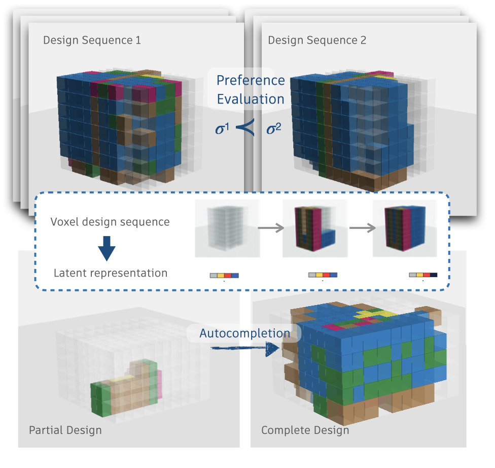
Figure 1: In this paper, we conduct representation learning for high-dimensional sequential volumetric design, and apply the learned representation for two downstream tasks: 1) preference evaluation over two design sequences (above) and 2) auto-completion with a partial design (below).

Many architectural design tasks are essentially sequential in nature, which requires numerous iterations and is often time-consuming. Additionally, there is a lack of tools that can help a designer with some initial realistic designs to make design iterations fast. Here we explore a learning-based approach for evaluating and generating complex design tasks. We specifically focus on the challenging task of sequential volumetric designs, a crucial step in professional building design. Volumetric design is a complex process that requires a multitude of manual efforts from expert designers. Several efforts have been made to automatically generate reasonable volumetric designs [5]. Unfortunately, the quality of the generated design solution varies, and evaluating a design solution requires either a prohibitively comprehensive set of metrics or expensive human expertise. Here our aim is to learn the underlying latent representation for such design tasks from a collection of high-performing sequential volumetric design data. We argue that this perspective on data-driven modeling of the sequential design procedure has several advantages due to the following reasons. First, from the workflow perspective, the existing solutions usually don’t reveal the decision-making process, which creates a barrier to human-AI interaction. Second, this idea opens up new possibilities to build AI-assisted sequential generative design tools that can incorporate expert feedback to fine-tune the design. Inspired by the success of Transformer-based models in the field of natural language processing (NLP) [4, 7] and computer vision (CV) [2, 14], we make the first endeavor to explore the idea of latent representation learning for sequential volumetric design, where the inputs are a sequence of voxel-based representations. Our key motivation is to use the learned representations for several crucial downstream tasks, such as reconstruction, preference evaluation, and auto-completion. We utilize self-attention layers from transformer models for these sequential tasks. To the best of our knowledge, this is one of the first attempts to encode design sequences into a latent representation and use multi-head self-attention-based models for design sequence generation. Our contributions can be summarized as the following:

• We present a novel ‘sequential volumetric design’ dataset and develop a self-attention-based encoder-decoder model to learn the latent representation of this dataset

• We demonstrate the effectiveness of the learned representations for autocompletion and reconstruction of design sequences

• We introduce and develop a preference model architecture that can provide preference over two volumetric design sequences by combining representation learning and flow-based density estimation

2 Related Work

Volumetric design and our proposed framework for learning representations span several topics such as 3D representation learning, density estimation, and high-dimensional sequential representation learning.

3D Representation Learning

3D shapes are commonly rasterized and processed into voxel grids for analysis and learning. Due to the correspondence and similarity between voxels and 2D pixels, many works have explored voxel-based classification and segmentation using volumetric convolution [23, 39, 40, 41, 44]. However, the volumetric convolution suffers from capturing rich context information with limited receptive fields. Recently, Transformer-based 3D backbones have proved to be a more effective architecture as long-range relationships between voxels can be encoded by the self-attention mechanism in the Transformer modules [24, 13]. Apart from 3D object detection and recognition, voxel-based latent generative models also have shown success for 3D shape generation [30, 38, 31, 33, 43]. However, voxel grids are memory-intensive. With the increase in dimensionality, voxel grids grow cubically, and thus, are expensive to scale to high resolution. Recently, interest in CAD-based representation learning has emerged due to the accessibility of large-scale datasets including collections of B-reps and program structure [19, 17], CAD sketches[21], and CAD assemblies[37, 36].

Density Estimation

Density estimation is heavily utilized in generative models to learn the probability density of a random variable, $p(x)$, given independent and identically distributed (i.i.d.) samples from it. Although density estimation allows sampling from a distribution or estimating the likelihood of a data point, this becomes challenging for high-dimensional data. Some popular approaches for high-dimensional density estimation include variational auto-encoder (VAE) [18], autoregressive density estimator [10], and flow-based models [9]. VAEs do not offer exact density evaluation and are often difficult to train. Autoregressive density estimators are sequential in nature and are trained autoregressively by maximum likelihood. An alternative approach, that we utilize in this study, is the normalizing flows which model the density as an invertible transformation of a simple reference density.

High-dimensional Sequential Representation Learning

Learning high-dimensional sequential representation, such as video frames, is challenging and has been widely studied with the transformer-based mechanism. With the prominent success of CLIP (Contrastive Language-Image Pre-training) [28], several methods have adopted and extended CLIP to video representation  [22, 20, 27, 1]. Learning meaningful state representations from visual signals is also essential for reinforcement learning (RL). A number of prior works have explored the use of auxiliary supervision in RL to learn such representations  [12, 16, 34]. Recently,  [42, 45] leverage transformer-based models to learn representation from consecutive video frames by using mask-based latent representation as the auxiliary objective, which can further improve the sample efficiency of RL algorithms.

Building Layout Generation & Analysis

Prior work on learning-based 3D building layout generation is rare. To the best of our knowledge, Building-GAN [5] is the only study exploring this direction where they train a graph-conditioned generative adversarial network (GAN) with GNN and pointer-based cross-model module to produce voxel-based volumetric designs. On the 2D layout generation, House-GAN [25] also proposes a graph-conditioned GAN, where the generator and discriminator are built on relational architecture. Similarly,  [8] uses multiple GAN modules to generate interior designs with doors, windows, and furniture. Layout-GMN [26] uses an attention-based graph matching network to predict structural similarity. Transformer-based neural network has also been studied in this field. HEAT [6] can reconstruct the underlying geometric structure with a given 2D raster image. HouseDiffusion [32] uses a diffusion model for vector-floorplan generation.

3 Methodology

3.1 Data Collection

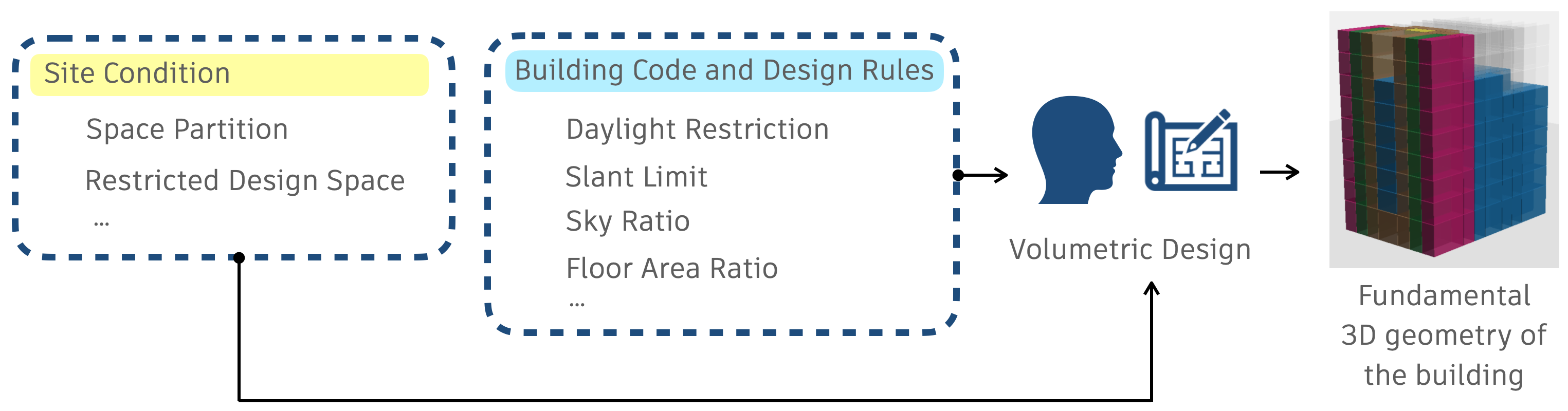
Figure 2: As the first critical step in professional building design, volumetric design takes into consideration of site condition, building code, and design rules (left). The outcome is a 3D structure where different colors represent different room types (right).

The volumetric design process usually performs in a given valid design space with several constraints, such as FAR and TPR. However, large collections of architectural volumetric designs are prohibitively expensive. For this reason, we opted for a heuristic agent built on top of [5] that can procedurally create a volumetric design based on several carefully created design principles defined by professional architects. The details of the design principles are described in the Appendix. Based on these design principles we develop Building-Gym, an OpenAI gym-like interface [3], that can produce a sequence of design states if actions are provided. Each design state, $s_{t}$, is a $10\times 10\times 10$ non-uniformed voxel space where each voxel has two channels to represent a) size and b) room type. We define seven room types: elevators, stairs, mechanical rooms, restrooms, corridors, office rooms, and non-existent rooms. For visualization purposes, each room type is color-coded. For example, as shown in Fig. 2, blue denotes office rooms and red denotes elevators. The color-coding details can be found in the Appendix. Our main motivation for developing Building-Gym is to provide a powerful sequential voxel building design simulator for researchers. Our initial dataset consists of $10^{4}$ optimal action sequences where each action sequence interacts with Building-Gym and produces a sequence of valid voxel design spaces that follow the design principles. An action sequence is of arbitrary length and can be represented by $(a_{0},a_{1},...,a_{T})$ where each action $a_{t}$ represents the location, size, and room type for each new voxel within the voxel space. In this way, using each action Building-Gym can provide us with a new design state. Next, we utilize these optimal action sequences to interact with Building-Gym and create $10^{4}$ sequences of voxel design spaces. Note that each sequence is a collection of high-performing voxel design spaces where each final state produces a diverse and valid voxel design space of a building. Fig. 3 shows how Building-Gym gradually creates a valid voxel design of a building using a sequence of actions.

3.2 Voxel design space to vector representation

To convert the voxel design spaces into neural network-friendly representations each state in the sequences is flattened into a $1000$-dimensional vector. We coin this design-to-vector representation as “design embedding”, $\mathbf{e}_{t}\in\mathbb{R}^{1000}$, which can be directly fed into the neural networks. Design embedding can be thought of as an analogy to word-to-vector representation in natural language processing. The process of generating one sequence of design embeddings is shown in Fig. 3. In the initial dataset $\mathcal{D}$, each design sequence has a length between $100$ and $810$. The distribution of the sequence length within $\mathcal{D}$ is shown below in Fig. 4. We found out that designs that are too short are not meaningful enough for any model to learn from. Thus we remove very short-length sequences from the dataset which results in a total number of $7296$ sequences. Based on our experiments, this dataset contains a diverse range of building designs and is sufficient to learn the sequential correlations in volumetric building design. We consider $6612$ sequences for training all the models reported in this paper and the other $684$ sequences for evaluation of the models. Finally, we sample design states from each sequence at a fixed frequency to truncate the sequence length into a more manageable value e.g. maximum length of $82$ instead of $800$. This sampling makes each sequence more interpretable by keeping the sequence size small and also makes the data processing pipeline more manageable.

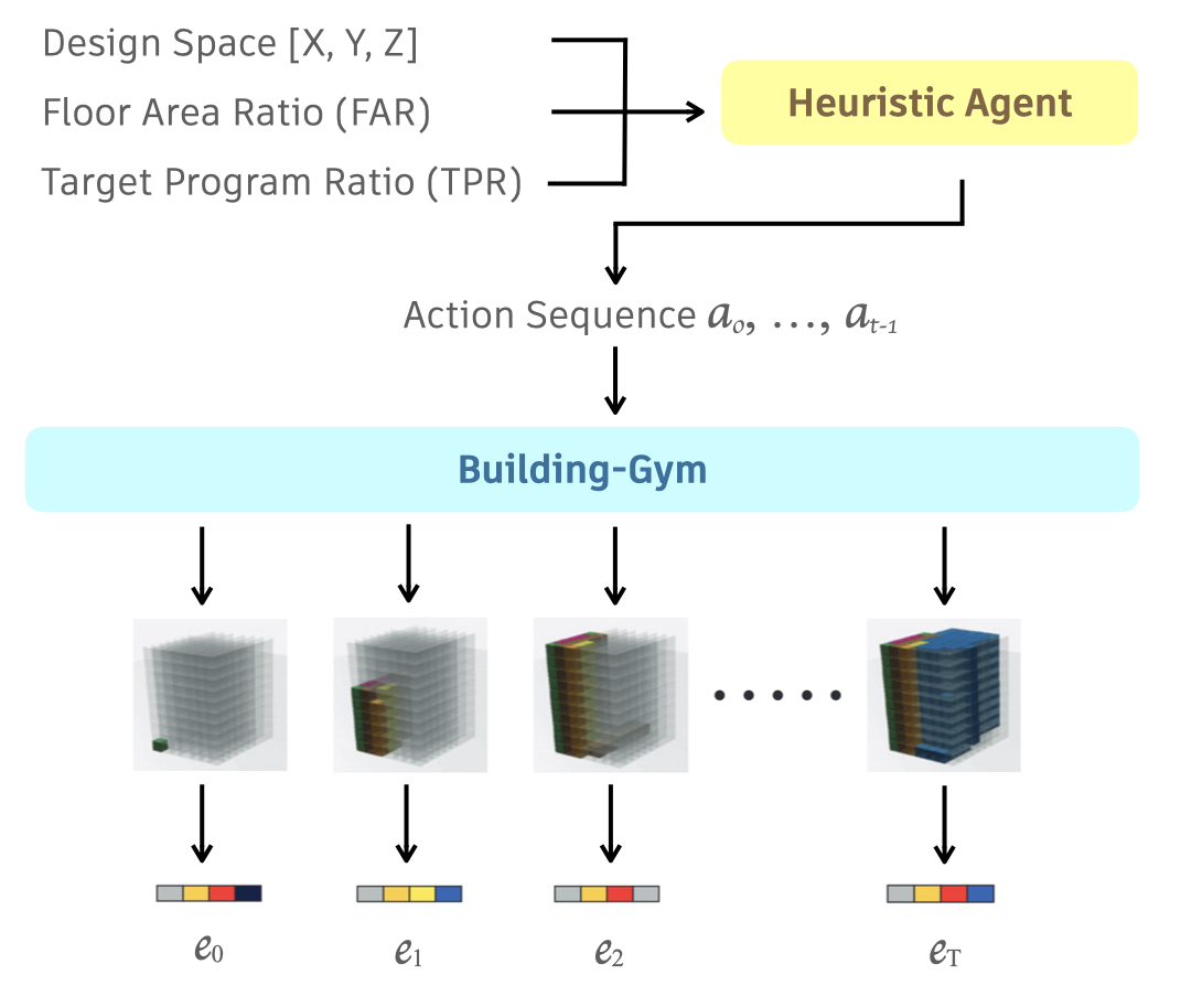
Figure 3: The pipeline to generate design embeddings: 1) our heuristic agent takes in a group of design constraints and outputs an action sequence for each design; 2) our Building-Gym environment takes in the action sequence and outputs a sequence of voxel-based design states, which are flattened into design embeddings.

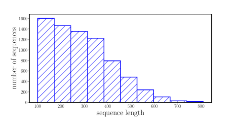
Figure 4: Distribution of sequence lengths in our dataset

3.3 Representation Learning for Sequential Design

Our main idea for learning effective representations of sequential design data is to estimate the density of the underlying latent space so that we can both sample data from the distribution and obtain the probability of a single data point. One straightforward way to estimate the density is to use likelihood-based models such as variational autoencoders [18]. In the case of VAE, the parameters of the posterior are jointly learned with the parameters of the decoder by minimizing the evidence lower bound (ELBO) loss:

$$\small\mathcal{L}(\theta,\phi)=\mathbb{E}_{z\sim q_{\theta}(\mathbf{z}|\mathbf{e})}\left[\log(p_{\phi}(\mathbf{e}|\mathbf{z}))\right]-\text{KL}(q_{\theta}(\mathbf{z}|\mathbf{e})||p(\mathbf{z}))\normalsize$$ (1)

where, $\mathbf{z}$ is the latent representation of the design embedding, $\mathbf{e}$, $p_{\phi}(\cdot)$ is the decoder parameterized by $\phi$, $q_{\theta}(\cdot)$ is the approximate posterior distribution parameterized by $\theta$, and $p(\mathbf{z})$ is the prior latent distribution. We consider a traditional zero mean and unit variance Gaussian prior, meaning $\mathbf{z}\sim\mathcal{N}(\mathbf{0},\mathbf{I})$ for each of the latent vectors of the sequence. One challenge with the likelihood-based model is that the regularization term on the right side of Eq. 1, often leads to poor accuracy of the model. To overcome such challenges, we propose to decouple density estimation from learning the latent representation. Thus we propose a two-step procedure; 1) learn the latent representation of the input sequences, and 2) estimate the density of the learned latent space.

Due to the sequential nature of the data, step 1 can be achieved using multi-head self-attention models such as transformers [35, 29]. To this end, we again consider two types of approaches for training the transformer-based models. The first approach is motivated by computer vision tasks where we try to reconstruct each design embedding in the sequence. Note that our goal is to reconstruct a whole sequence, unlike the traditional approaches where only a single design is reconstructed for learning the latent representations. In this way, the transformer model would take an input sequence of design embeddings $(\mathbf{e}_{0},\mathbf{e}_{1},\dots,\mathbf{e}_{T})$ and predict $(\hat{\mathbf{e}}_{0},\hat{\mathbf{e}}_{1},\dots,\hat{\mathbf{e}}_{T})$ where $\mathbf{e}_{t}$ is the $t$-th design embedding of the sequence. Our second approach is motivated by NLP tasks, where we consider autoregressively predicting each design embedding sequentially. The objective can be expressed as maximizing the conditional probability, $\text{arg max}_{\theta}p(\mathbf{e}_{t}|\mathbf{e}_{0},\mathbf{e}_{1},\dots,\mathbf{e}_{t-1};\theta)$, with respect to some parameter $\theta$.

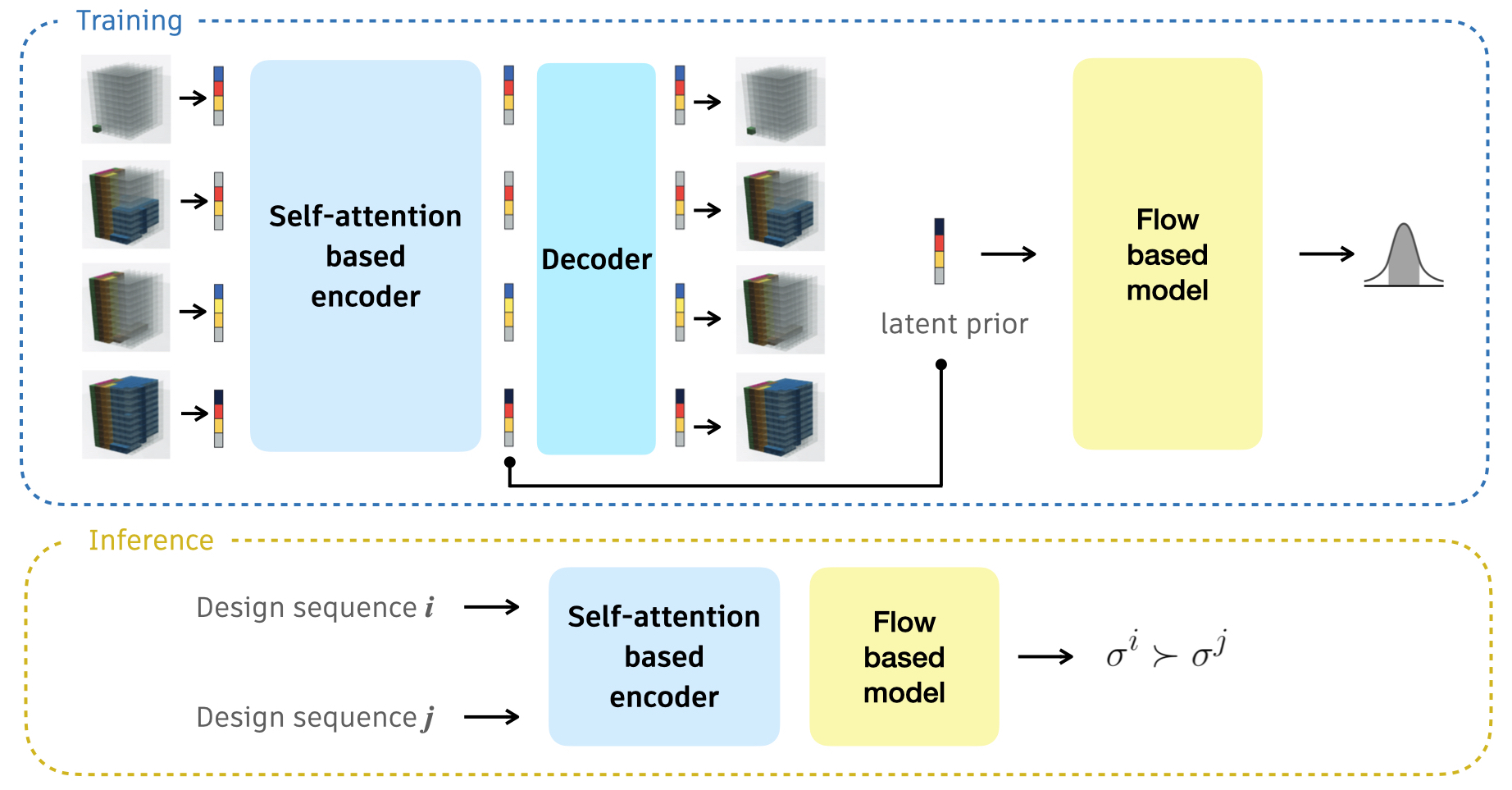
Figure 5: We develop an encoder-decoder based model for learning representations of sequential volumetric design data. The encoder portion consists of multi-head self-attention architectures. The output from the final self-attention layer is used to further train a flow-based model, e.g. real NVP for density estimation. Note that we keep the weights of the encoder frozen while training the flow model. During inference time, weights of both the encoder and the flow model are kept frozen to obtain the log-likelihood of a design sequence. Directly comparing this log-likelihood provides preference of design sequence $\sigma^{i}$ over design sequence $\sigma^{j}$.

We train the transformer models using the reconstruction loss or the next design embedding prediction loss and extract the latent representations $(\mathbf{z}_{0},\mathbf{z}_{1},\dots,\mathbf{z}_{T})$, where $\mathbf{z}_{t}\in\mathbb{R}^{2048}$, of each sequence $(\mathbf{e}_{0},\mathbf{e}_{1},\dots,\mathbf{e}_{T})$ from the final self-attention layer. Positional encoding is also used before feeding the input to these attention layers. Next, we use the trained latent vectors as prior $p(\mathbf{z})$ to further train a flow-based model, e.g real NVP [18], for estimating the density. We choose flow-based models because they can work with high dimensional density estimation problems. Here we only use $\mathbf{z}_{T}$ to train the flow model although any number of latent vectors can be used by concatenating them. We consider that the latent code of the final state, $\mathbf{z}_{T}$, encodes information of the whole sequence because all of the previous states of a sequence contribute to this final and completed voxel design. Our proposed framework is illustrated in the training section of Fig. 5.

3.4 Preference Model via Density Estimation

As an important downstream application of the learned representations, we develop preference models for volumetric designs. The core idea of a preference model is to assign preference between two input designs. This can be used in getting feedback to align a generative design model for desired user specifications. Our preference model consists of a pre-trained self-attention model and a pre-trained flow-based model. First, an input design sequence is passed through the pre-trained self-attention model. Second, output from the last attention layer is passed through the pre-trained flow-based model to achieve the log-likelihood. In this study, we only use the final latent vector of the sequence as it already contains information about the previous timesteps. In this way, we can obtain the log-likelihood of two input design sequences and compare them to provide preference.

$$\small\text{preference}=\begin{cases}\sigma^{i}\succ\sigma^{j}&\text{if }\log p(\mathbf{z}_{i})>\log p(\mathbf{z}_{j})\\ \sigma^{i}\prec\sigma^{j}&\text{if }\log p(\mathbf{z}_{i})<\log p(\mathbf{z}_{j})\end{cases}\normalsize$$ (2)

Note that we use the notation $\sigma^{i}\succ\sigma^{j}$ to represent the preference of design sequence $i$ over design sequence $j$. Intuitively, this is equivalent to saying that the design sequence $i$ is more realistic than the design sequence $j$. The process is illustrated in the Inference section of Fig. 5. As a baseline, we also develop a simple VAE-based preference calculation procedure and compare it against the proposed preference model. For this baseline, we train a VAE by minimizing Eq. 1 which gives us the posterior of the latent space regularized towards the mean of the prior. For an input design sequence, we calculate the distance between the last latent vector of the sequence and the mean, $\mu$, of the prior. Next, we compare the distances between two input design sequences to identify the preference.

$$\small\text{VAE-preference}=\begin{cases}\sigma^{i}\succ\sigma^{j}&\text{if }||\mathbf{z}_{i}-\mu||<||\mathbf{z}_{j}-\mu||\\ \sigma^{i}\prec\sigma^{j}&\text{if }||\mathbf{z}_{i}-\mu||>||\mathbf{z}_{j}-\mu||\end{cases}\normalsize$$ (3)

3.5 Building Design Autocompletion

As a second downstream application of the learned representations, our goal is to feed a partial sequence to a model as input and obtain a completed sequence of a design. This happens in an auto-regressive manner where each design state depends on all the previous states of that design sequence and is thus predicted auto-regressively. Unlike language models, the raw output of the auto-regressive model cannot be used for volumetric designs as it is not possible to map the embedding to a specific design state. We identify this as a major challenge for generative architectural design models. To make sure that each generated design state follows the previous states, we use an additional mapping layer $\phi$, that ensures that no existing room from the previous state gets deleted although the room type can be changed. Note that when the model autocompletes the structure of the building we allow it to change the room types for generating diverse designs that are different from the training data. If $Dec$ is the decoder, $Enc$ is the self-attention-based encoder, $\phi$ is the mapping layer, and $\mathbf{e}_{t}$ is the $t$-th design embedding of the sequence then we can write the following, $\mathbf{e}_{t}=\phi((\hat{\mathbf{e}}_{t}))$ where $\hat{\mathbf{e}}_{t}=Dec(Enc(\mathbf{e}_{t-1}))$. Finally each embedding is converted back to a design state for voxel space representation. Evaluating these generated designs is challenging as we cannot compare them against the ground truth similar to the reconstruction task. To this end, we propose “sequential FID” scores for evaluating generated designs. This idea is an extension of the traditional image generation evaluation using the “Fréchet Inception Distance”(FID) score [15] in the sequential setting. The key idea is to obtain the Gaussian distribution of the $t$-th generated design embedding with mean, $\mathbf{m}_{w,t}$ and variance, $\mathbf{C}_{w,t}$ and compare them against the Gaussian distribution of the $t$-th design embedding from the training dataset with mean $\mathbf{m}_{t}$, and variance $\mathbf{C}_{t}$ using the following formula,

$$\begin{split}f_{t}(&(\mathbf{m}_{t},\mathbf{C}_{t}),(\mathbf{m}_{w,t},\mathbf{C}_{w,t}))=||\mathbf{m}_{t}-\mathbf{m}_{w,t}||_{2}\\ &+\text{Tr}\left(\mathbf{C}_{t}+\mathbf{C}_{w,t}-2(\mathbf{C}_{t}\mathbf{C}_{w,t})^{1/2}\right).\end{split}$$ (4)

We calculate the FID score sequentially for all of the design embeddings of the sequence.

4 Experiment and Result

4.1 Model Implementation and Training Details

For the encoder part of our models, we use a GPT2-like structure which has several self-attention layers with multiple heads. Based on our experiments, we choose four self-attention layers and eight attention heads to run all of the experiments reported in this paper. We use a projection layer before the self-attention layers in our architecture. Additionally, the input sequence is masked in the usual way so that future states are not available to the model. For the decoder part of our model, we use a simple linear layer and then a sigmoid layer to keep the predicted values between $0$ and $1$. We train two different versions of this model: one for reconstructing each design embedding, which we call the ‘Volumetric Design Reconstruction (VDR)’ model, and one for predicting the next design embedding from the current embeddings, which we call the ‘Autoregressive Volumetric Design (AVD)’ model. Each model is trained using stochastic gradient descent and binary cross-entropy loss. In the case of the flow-based model, we train a real NVP flow model with five coupling layers and a hidden dimension of $2048$.

4.2 Reconstruction

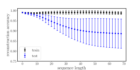
Figure 6: Reconstruction accuracy of training and evaluation dataset using the ‘Volumetric Design Reconstruction’ (VDR) model

As described in the previous section, we train two models to learn the latent representations of the volumetric design data. The ‘Volumetric Design Reconstruction (VDR)’ model is used to reconstruct each design embedding. Fig. 6 shows the reconstruction accuracy for both the training and evaluation datasets. As shown in the figure, the average reconstruction accuracy over the entire sequence is close to $100\%$ for the training data. This is impressive considering the fact that the model can generalize over a large range of volumetric design sequences. For the evaluation dataset, the model can achieve more than $80\%$ reconstruction accuracy, but it becomes less accurate over the longer timesteps. We hypothesize that including diverse designs in the training data may improve the evaluation accuracy and provide better generalization for design tasks. We conduct an ablation study on the number of attention layers and heads. The results are listed in Table 1. Different layers and heads don’t show significant differences in the reconstruction accuracy. Finally, we visualize two sequences and their corresponding reconstructed designs using our VDR model in Fig. 15 and 16. The qualitative results match the trend in Fig 6, where some errors are introduced in the later steps from the evaluation data. However, the structure of the building and the majority of the room types are still preserved. More qualitative results can be found in the Appendix.

Layers	Heads	Reconstruction accuracy
		Training	Evaluation
$4$	$2$	$99.34\%+0.0063$	$92.26\%+0.0656$
$4$	$4$	$99.24\%+0.0074$	$92.11\%+0.0660$
$4$	$8$	$99.27\%+0.0069$	$92.23\%+0.0661$
$8$	$2$	$99.34\%+0.0066$	$89.71\%+0.0758$
$8$	$4$	$99.30\%+0.0071$	$89.74\%+0.0758$
$8$	$8$	$99.26\%+0.0078$	$89.80\%+0.0758$

Table 1: Comparison between various model architectures for reconstruction accuracy for both training and evaluation dataset

\begin{overpic}[width=74.52539pt,unit=1pt]{figures/S_0_T_1_GT.png} \put(-15.0,2.0){\rotatebox{90.0}{\scriptsize Ground Truth}} \end{overpic}
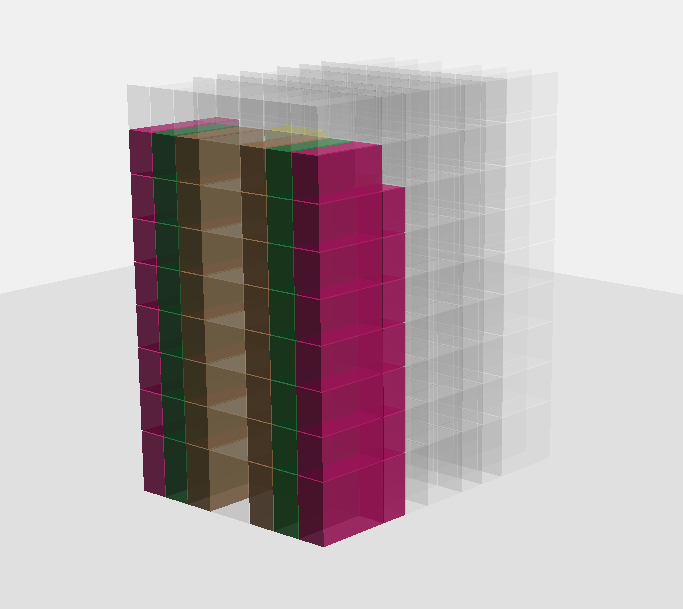
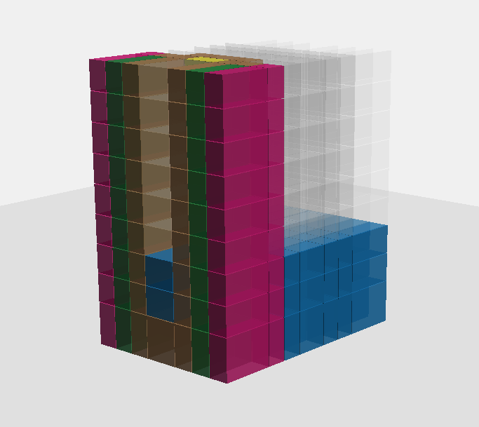
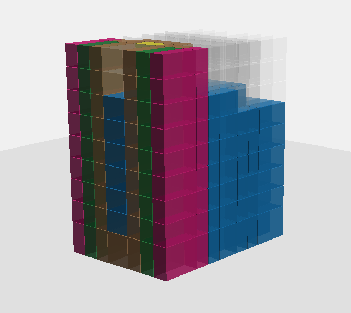
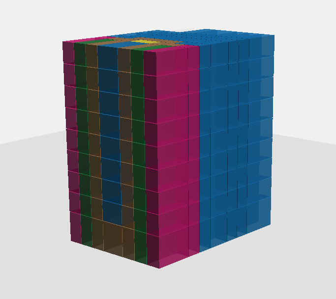
\begin{overpic}[width=74.52539pt,unit=1pt]{figures/S_0_T_1.png} \put(-15.0,2.0){\rotatebox{90.0}{\scriptsize Reconstruction}} \put(65.0,3.0){{\scriptsize$t=0$}} \end{overpic}	\begin{overpic}[width=74.52539pt,unit=1pt]{figures/S_0_T_2.png} \put(65.0,3.0){{\scriptsize$t=12$}} \end{overpic}	\begin{overpic}[width=74.52539pt,unit=1pt]{figures/S_0_T_3.png} \put(65.0,3.0){{\scriptsize$t=24$}} \end{overpic}	\begin{overpic}[width=74.52539pt,unit=1pt]{figures/S_0_T_4.png} \put(65.0,3.0){{\scriptsize$t=36$}} \end{overpic}	\begin{overpic}[width=74.52539pt,unit=1pt]{figures/S_0_T_5.png} \put(65.0,3.0){{\scriptsize$t=45$}} \end{overpic}

Figure 7: Reconstruction of a design sequence (below) from the training data and compare with the ground truth (above).

\begin{overpic}[width=74.52539pt,unit=1pt]{figures/S_5_T_1_GT.png} \put(-15.0,2.0){\rotatebox{90.0}{\scriptsize Ground Truth}} \end{overpic}
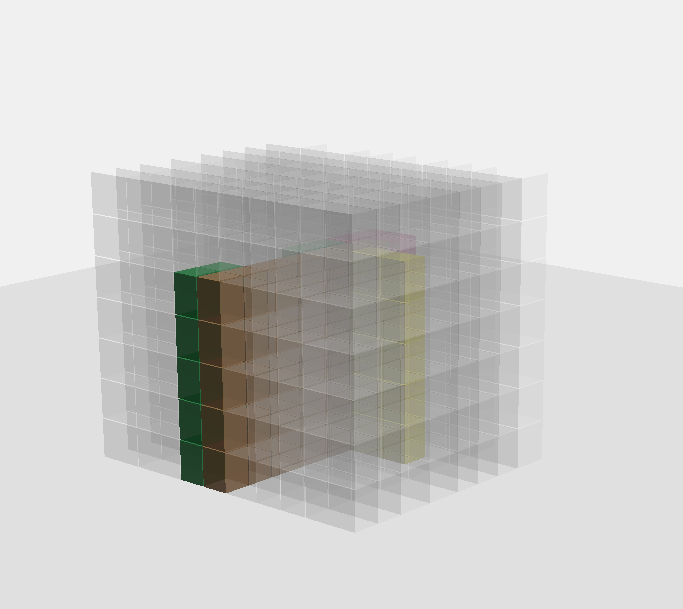
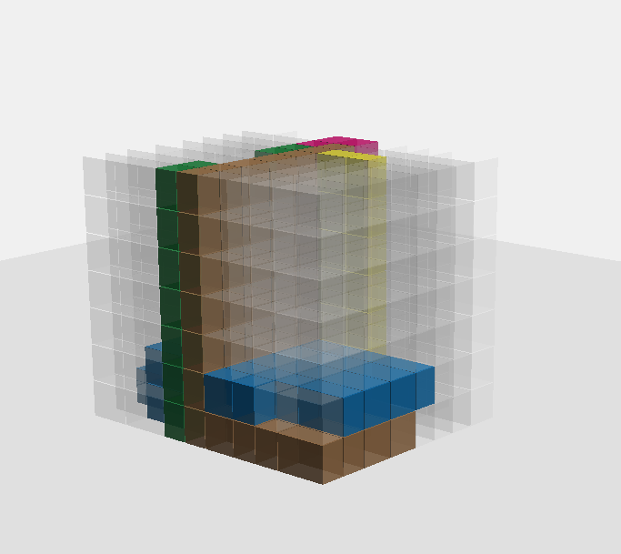
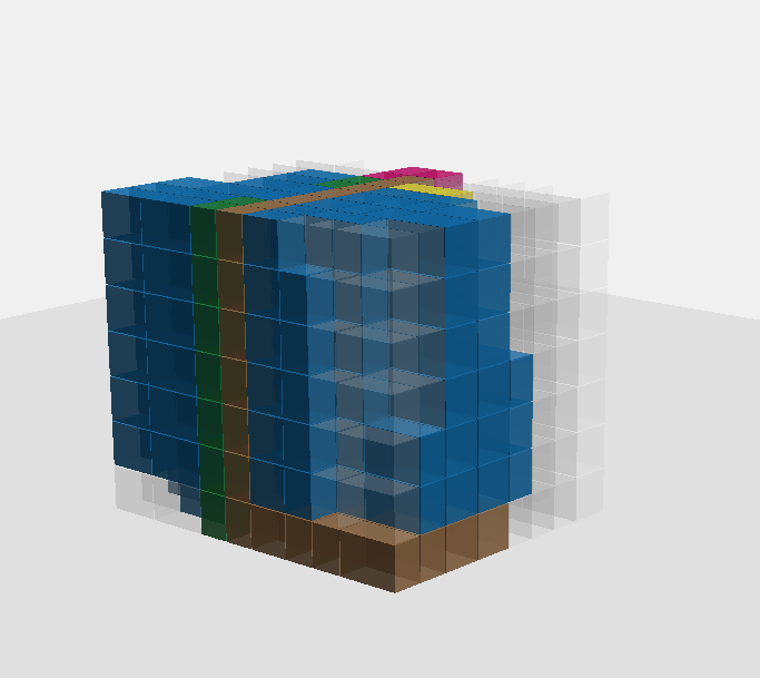
\begin{overpic}[width=74.52539pt,unit=1pt]{figures/S_5_T_1.png} \put(-15.0,2.0){\rotatebox{90.0}{\scriptsize Reconstruction}} \put(65.0,3.0){{\scriptsize$t=0$}} \end{overpic}	\begin{overpic}[width=74.52539pt,unit=1pt]{figures/S_5_T_2.png} \put(65.0,3.0){{\scriptsize$t=12$}} \end{overpic}	\begin{overpic}[width=74.52539pt,unit=1pt]{figures/S_5_T_3.png} \put(65.0,3.0){{\scriptsize$t=24$}} \end{overpic}	\begin{overpic}[width=74.52539pt,unit=1pt]{figures/S_5_T_4.png} \put(65.0,3.0){{\scriptsize$t=36$}} \end{overpic}	\begin{overpic}[width=74.52539pt,unit=1pt]{figures/S_5_T_5.png} \put(65.0,3.0){{\scriptsize$t=45$}} \end{overpic}

Figure 8: Reconstruction of a design sequence from the evaluation data (below) and compare with the ground truth (above).

\begin{overpic}[width=74.52539pt,unit=1pt]{figures/S_86_T1_GT.png} \put(-15.0,2.0){\rotatebox{90.0}{\scriptsize Ground Truth}} \end{overpic}
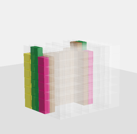
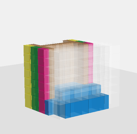
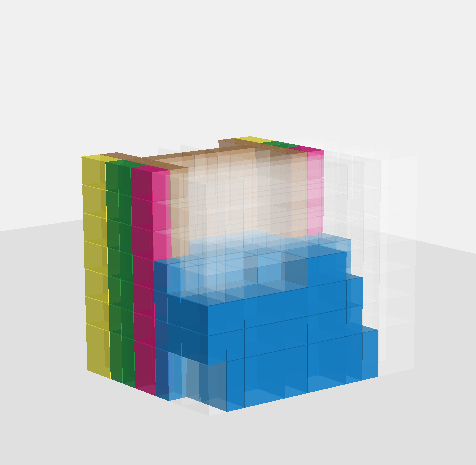
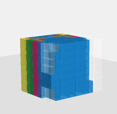
\begin{overpic}[width=74.52539pt,unit=1pt]{figures/S_86_T1.png} \put(-15.0,2.0){\rotatebox{90.0}{\scriptsize Autocompletion}} \put(65.0,3.0){{$t=0$}} \end{overpic}	\begin{overpic}[width=74.52539pt,unit=1pt]{figures/S_86_T2.png} \put(65.0,3.0){{\scriptsize$t=8$}} \end{overpic}	\begin{overpic}[width=74.52539pt,unit=1pt]{figures/S_86_T3.png} \put(65.0,3.0){{\scriptsize$t=12$}} \end{overpic}	\begin{overpic}[width=74.52539pt,unit=1pt]{figures/S_86_T4.png} \put(65.0,3.0){{\scriptsize$t=18$}} \end{overpic}	\begin{overpic}[width=74.52539pt,unit=1pt]{figures/S_86_T5.png} \put(65.0,3.0){{\scriptsize$t=27$}} \end{overpic}

Figure 9: Autocompletion with a partial design given at t=0 from the training data (below) and compare with the ground truth (above).

\begin{overpic}[width=74.52539pt,unit=1pt]{figures/S_43_T1_GT.png} \put(-15.0,2.0){\rotatebox{90.0}{\scriptsize Ground Truth}} \end{overpic}
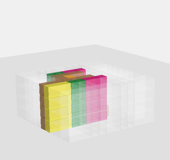
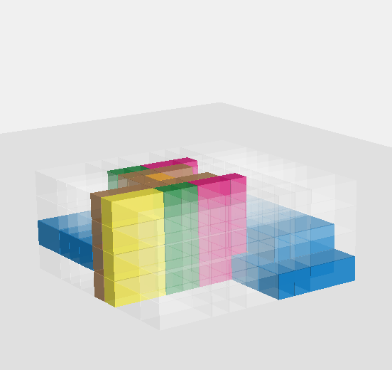
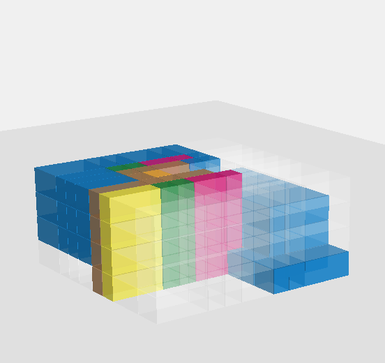
\begin{overpic}[width=74.52539pt,unit=1pt]{figures/S_43_T1.png} \put(-15.0,2.0){\rotatebox{90.0}{\scriptsize Autocompletion}} \put(65.0,3.0){{\scriptsize$t=0$}} \end{overpic}	\begin{overpic}[width=74.52539pt,unit=1pt]{figures/S_43_T2.png} \put(65.0,3.0){{\scriptsize$t=5$}} \end{overpic}	\begin{overpic}[width=74.52539pt,unit=1pt]{figures/S_43_T3.png} \put(65.0,3.0){{\scriptsize$t=10$}} \end{overpic}	\begin{overpic}[width=74.52539pt,unit=1pt]{figures/S_43_T4.png} \put(65.0,3.0){{\scriptsize$t=15$}} \end{overpic}	\begin{overpic}[width=74.52539pt,unit=1pt]{figures/S_43_T5.png} \put(65.0,3.0){{\scriptsize$t=20$}} \end{overpic}

Figure 10: Autocompletion with a partial design given at t=0 from the evaluation data (below) and compared with the ground truth (above).

4.3 Preference Model

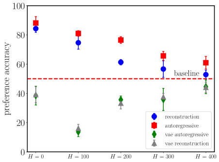
Figure 11: Preference accuracy of the Autogressive Volumetric Design (AVD) model and the Volumetric Design Reconstruction (VDR) model are shown with one standard deviation range, preference accuracy from the two types of VAE models are also shown; one for reconstruction and one for autoregressive prediction

To evaluate the performance of the preference model, we create five different versions of the evaluation datasets that each consist of $684$ sequences of volumetric designs. This is done by following the heuristic agent until a fixed horizon length, $H$, and then following a random policy for designs. This means that $H=0$ are completely random designs, and $H=400$ are close to expert designs. We choose $H=0,100,200,300,400$ to gradually make the designs less random. Some examples of each evaluation dataset are shown in the appendix. The results of this test are shown in Fig. 11. As the designs become closer to the expert designs, the accuracy of our preference model decreases. This aligns with our expectations because the correlation within the design sequence becomes very close to the ground truth.

Additionally, we find that the learned representations from the AVD model provide better preference accuracy compared to the VDR model. This might be due to the fact that the autoregressive models can capture the correlation between design embeddings over the entire sequence, unlike the reconstruction model. The preference accuracy obtained using AVD is close to $90\%$ against completely random designs. For less random designs, the preference accuracy drops almost linearly. Note that for the $H=400$ dataset, the preference score is close to $60\%$. This can be explained by the fact that most design sequences become very close to the ground truth in this case and thus the preference becomes almost random. For the VDR model, we observe similar but slightly less preference accuracy. The highest preference accuracy is close to $85\%$ in this case and this happens against completely random designs. On the other hand, the preference accuracy of the VAE-based model is significantly lower than both the AVD and VDR models. This directly follows our intuitions from section 3.4. Intuitively, this represents the difficulties of learning a useful latent posterior using the ELBO loss in 1 for volumetric designs.

4.4 Autocompletion

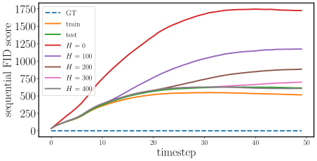
Figure 12: Comparing generated design sequences and random design sequences based on sequential FID scores to the ground truth for each timestep.

During inference time, we feed a partial input sequence of length $5$ to the AVD model and sequentially predict the next embeddings until a fixed timestep of length $50$. We demonstrate the qualitative design generation capability of AVD in Fig. 17 and Fig.18 where the partial design input comes from the training and evaluation dataset respectively. For the first case, it is easy to notice that the autocompleted design follows the ground truth very closely with some minor variations. However, for the previously unseen input, the autocompleted design is diverse when compared to the ground truth. Although the structure of the design seems realistic, the room types are not assigned correctly for a realistic volumetric design. We suspect that this happens because the autoregressive model cannot properly capture the complex correlation between different room types. For a quantitative evaluation of the autocompleted sequences, we calculate the sequential FID score using equation 4. We feed all the training data through the trained self-attention encoder and use the output latent vectors to calculate the mean and variance. This is shown in Fig. 12 where we also compare the sequential FID scores against various levels of randomness in the design sequences, $H=0,H=100,H=200,H=300,H=400$. The interpretation of this result is that the autoregressive model can generate designs that are more realistic than a random design sequence. The sequential FID scores are very close to the optimal design sequences, $H=400$, which justifies the credibility of the generated design sequences. Also, note that the FID scores increase for random design sequences which makes sense due to the randomness of each design state.

5 Discussion & Future Work

We investigate the use of transformer-based models for learning representations of high-dimensional sequential volumetric design data. This is an important step toward developing data-driven models for evaluating and generating sequential design tasks. Our models can successfully reconstruct designs sequentially and accurately evaluate two design sequences with a trained flow-based density estimation model. We also examine auto-completion with our models, but the results are not satisfying. We believe this results from the complex spatial correlation between the room types in each volumetric design. As we sampled states from the original sequence to reduce the sequence length, it might have affected the sequential generation capabilities of the model. Additionally, the sequential design generation task is somewhat different from natural language processing tasks as there is no token associated with a building design state. Instead, our model is trying to directly predict the design embedding at each timestep. A potential solution might be to use carefully designed model architectures that can map the design embedding to a design state from a finite set of states. As this is one of the earliest studies on sequential design generation and design preference model building, we expect it to open new directions for research in this domain. Some future works include 1) developing metrics to better evaluate the quality of generated designs; 2) utilizing the preference model in a reinforcement learning framework to serve as a reward function engine, and 3) incorporating latent space searching methods (such as [11]) to not only generate plausible designs but also optimize for specific design objectives. The use of self-attention based architecture to capture sequential design decisions opens up possibilities of carrying over various methods and results from natural language processing to design domains.

6 Supplementary material

6.1 Heuristic Agent for Expert Design

Together with professional architects, we design a heuristic agent to generate expert designs. Here we describe the general principles of the heuristic agent:

1. Generating an empty non-uniformed 3D partition space $[X,Y,H]$;

2. Based on the partition, FAR, TPR, determining the number of elevators;

3. Positioning the elevators on the first floor to make sure they are symmetric to each other. For example, if only one elevator, then it should be placed in the center; if two elevators, they should be placed at two diagonal corners, etc.

4. Positioning service rooms (stairs, mechanical rooms, and restrooms) around the elevators;

5. Generating corridors to connect the above rooms;

6. Duplicating the above layout to each floor to make sure they are vertically aligned;

7. Growing a lobby on the first floor until FAR & TPR are satisfied; keeping the shape as rectangular as possible;

8. Growing office rooms on the second floor until FAR & TPR are satisfied; keeping the shape as rectangular as possible;

9. Duplicating the layout of the second floor to the rest of the floors;

Table 2: Color coding for different room types used throughout this paper

room type	color
office	blue
elevator	green
stairs	yellow
restroom	pink
Lobby	brown
Mechanical	orange

6.2 Additional Dataset Statistics

Here we show the distribution of the floor-to-area (FAR) ratio values in Fig. 13 and the distribution of the average number of rooms per floor in Fig. 14.

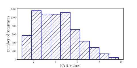
Figure 13: Distribution of FAR values in the volumetric design dataset

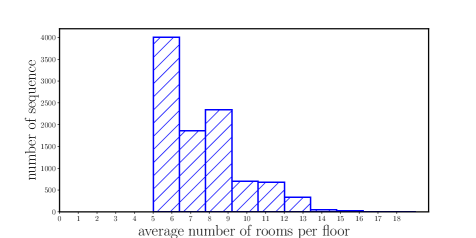
Figure 14: Distribution of the average number of rooms per floor in the volumetric design dataset

6.3 Additional Qualitative Results

Here we show some additional visualization of reconstructing sample sequences from both the training data and the evaluation data in figure 15 and 16, respectively. We also show some autocompleted design sequences from partial input designs from both the training data and the evaluation data in figure 17 and 18, respectively. We compare each design sequence against the ground truth. Finally, we visualize some sample sequences from the five different degrees of random datasets used to evaluate the preference model in figure 19.

		Ground Truth
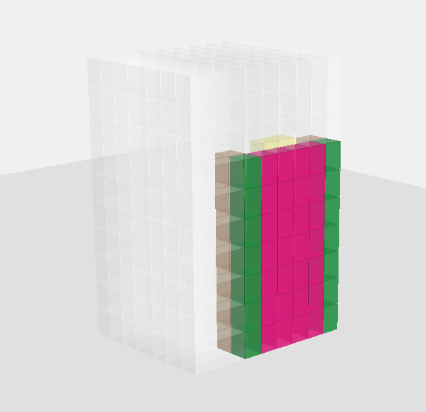
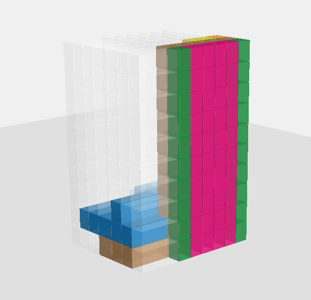
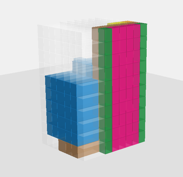
		Reconstruction
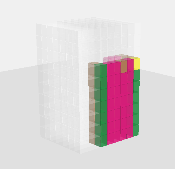
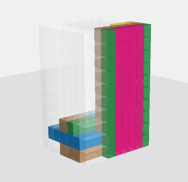
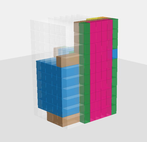
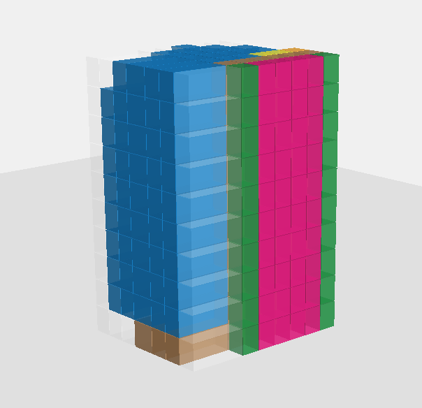
		(1)
		Ground Truth
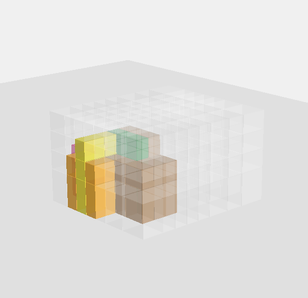
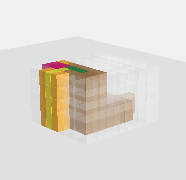
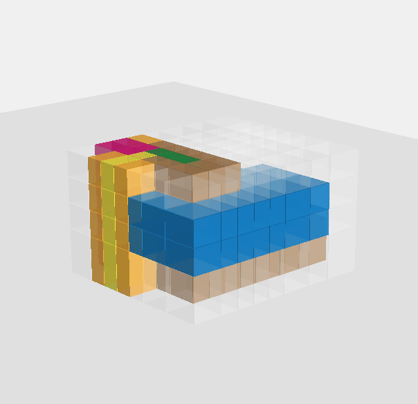
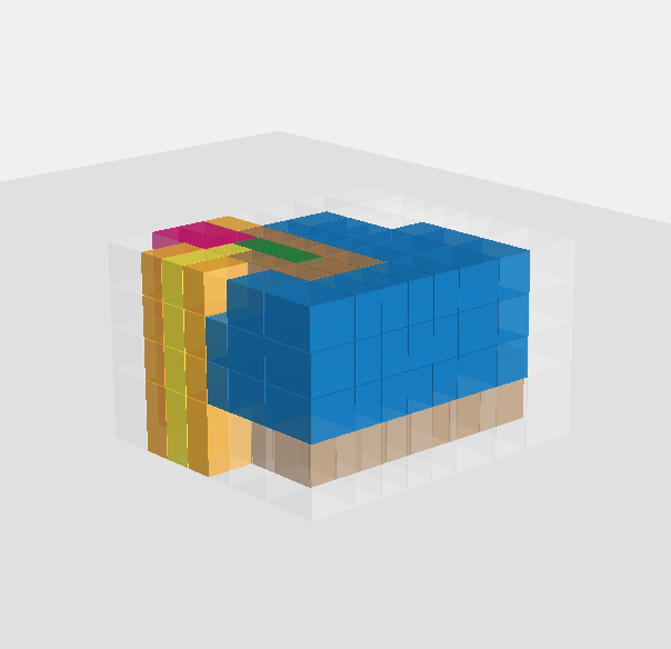
		Reconstruction
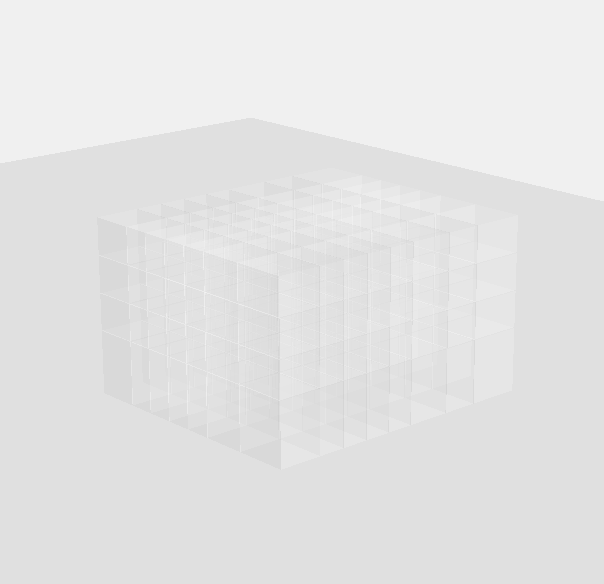
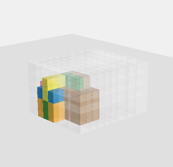
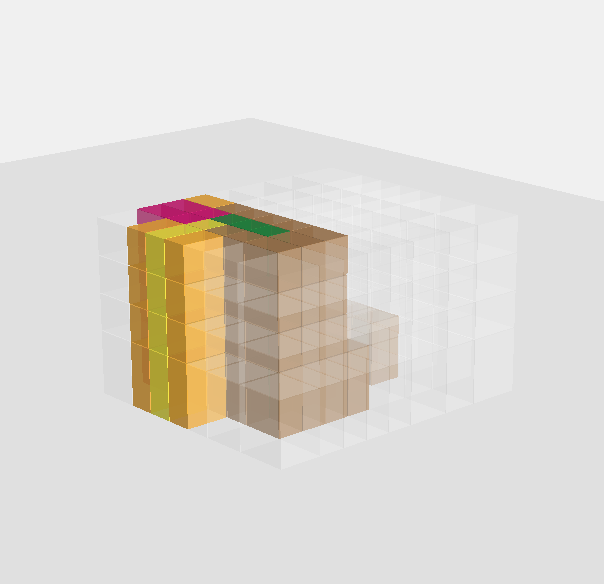
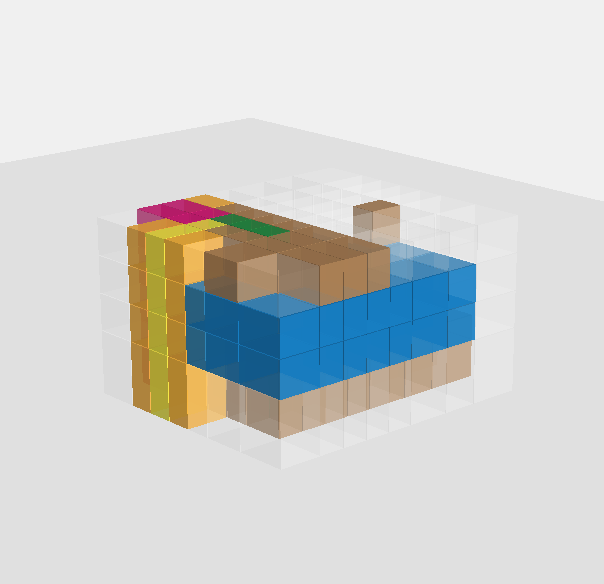
		(2)
		Ground Truth
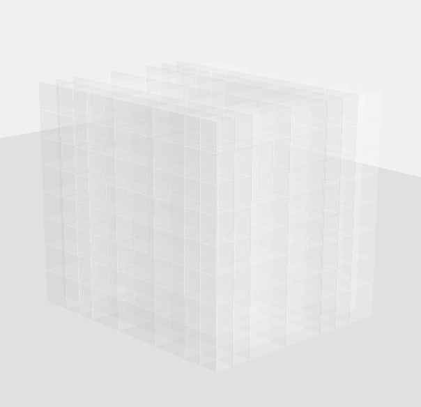
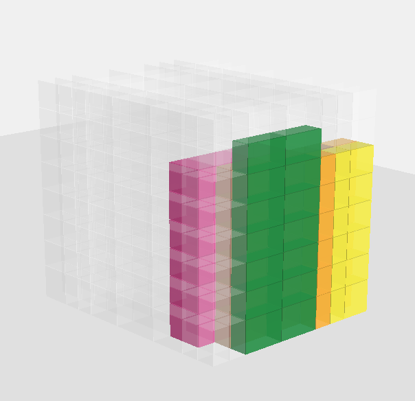
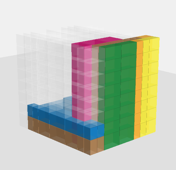
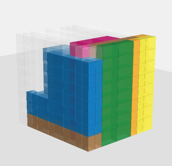
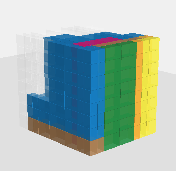
		Reconstruction
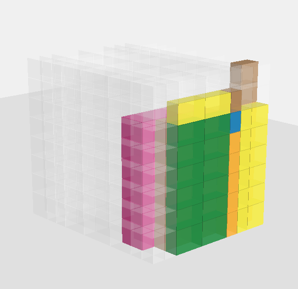
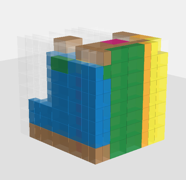
		(3)

Figure 15: Reconstruction: design reconstruction of sample sequences from the training data and comparison with the ground truth.

.

		Ground Truth
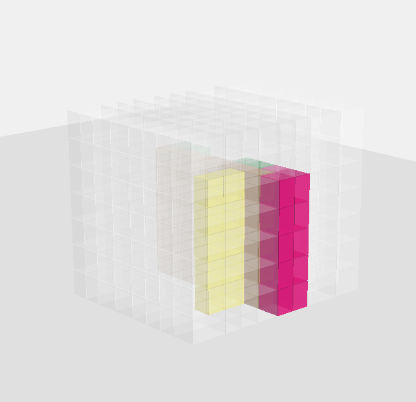
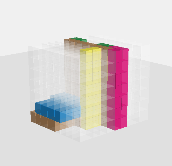
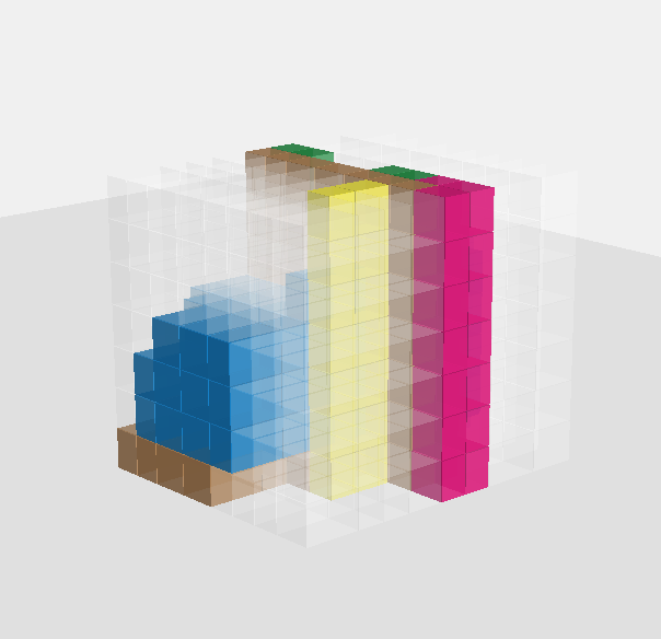
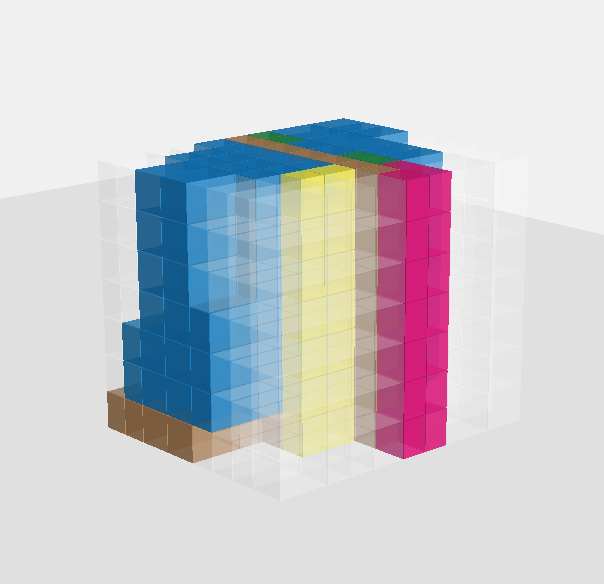
		Reconstruction
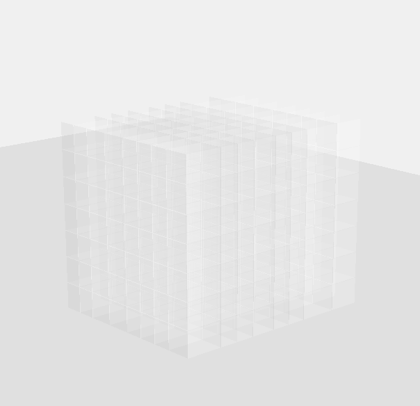
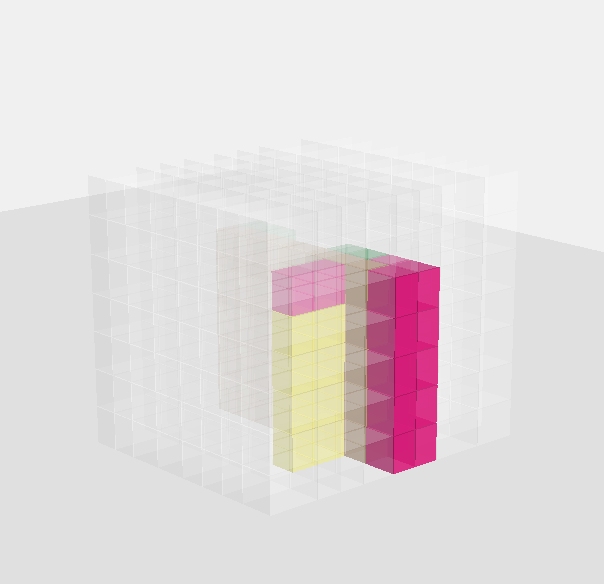
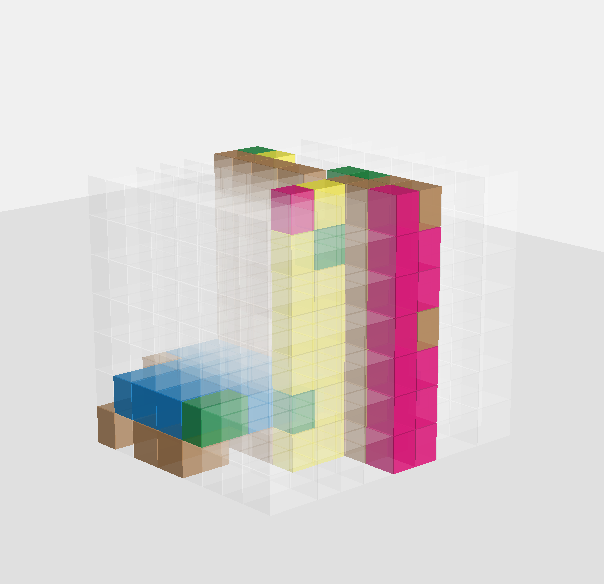
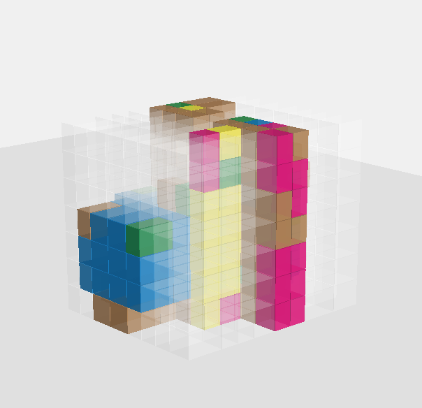
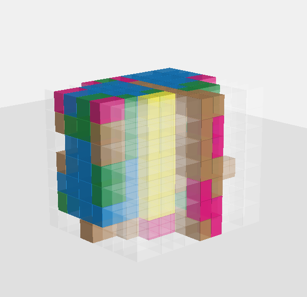
		(1)
		Ground Truth
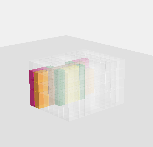
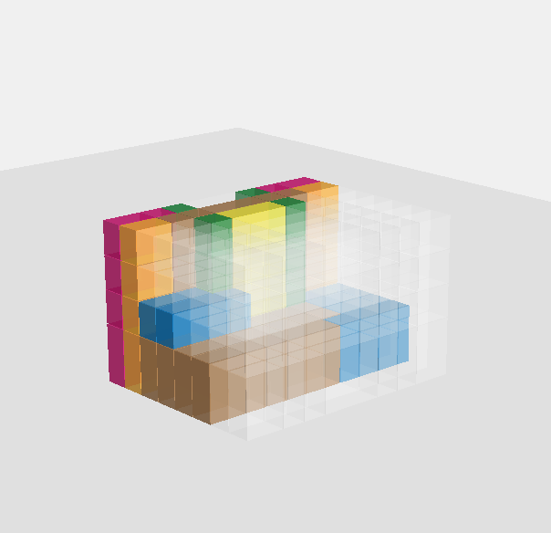
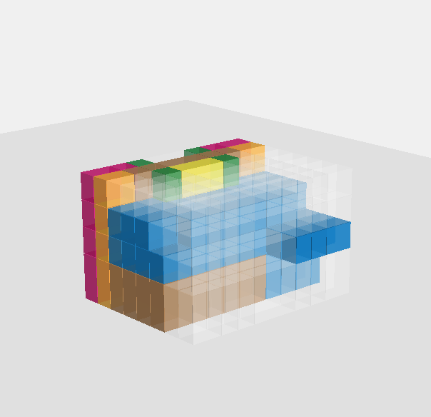
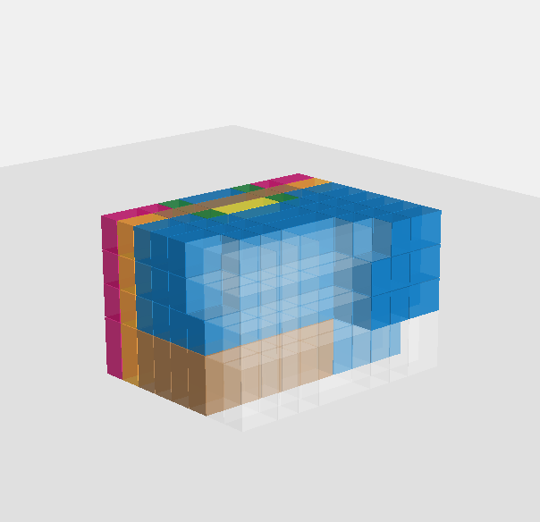
		Reconstruction
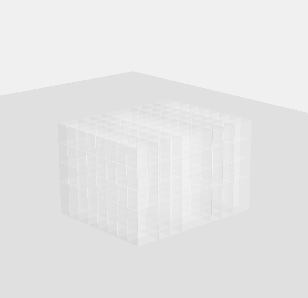
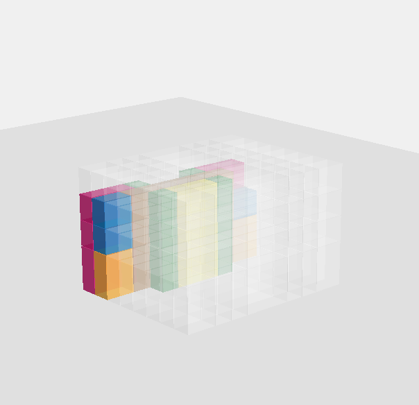
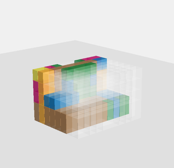
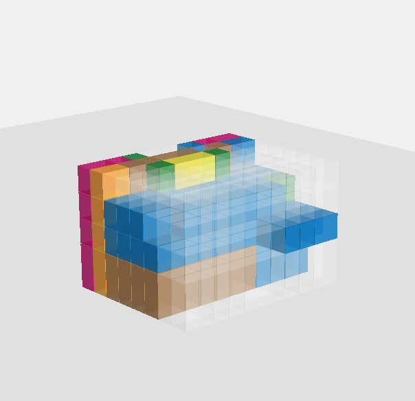
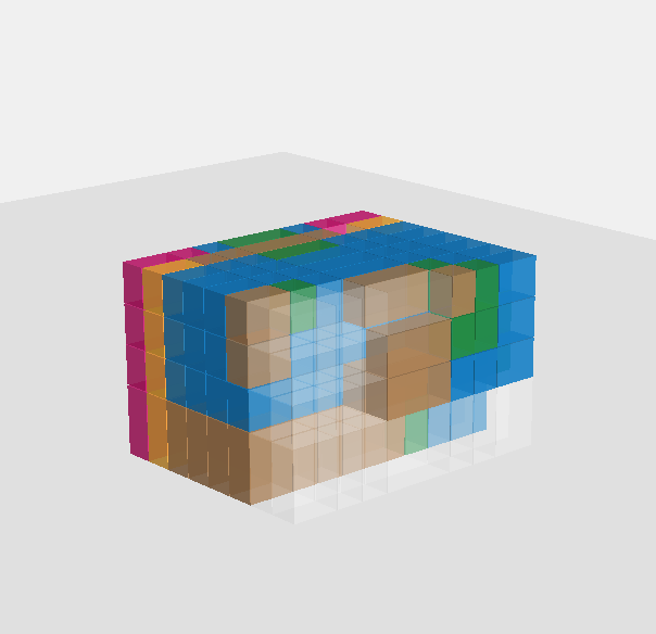
		(2)
		Ground Truth
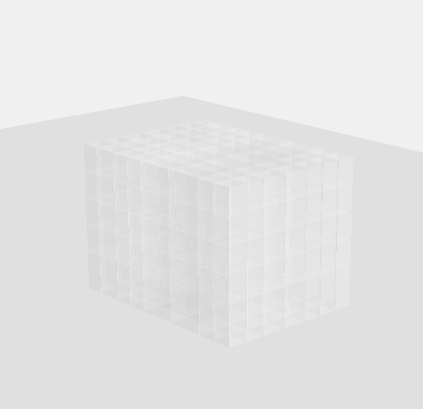
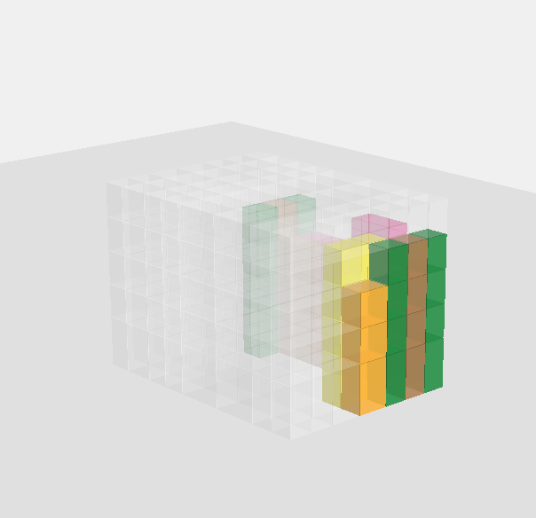
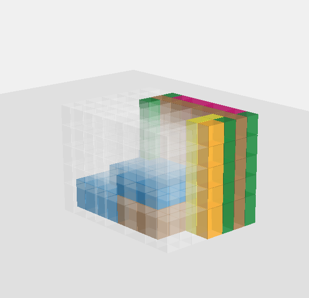
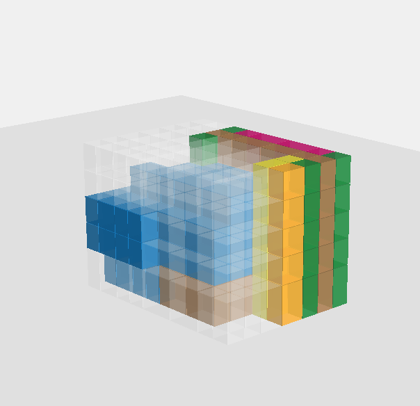
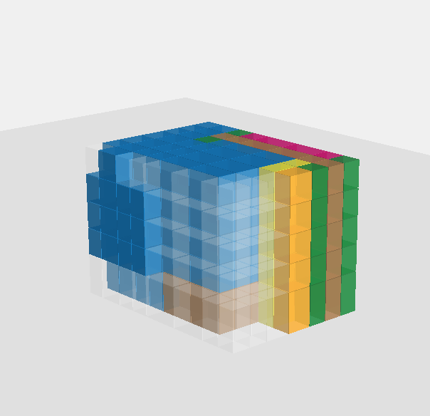
		Reconstruction
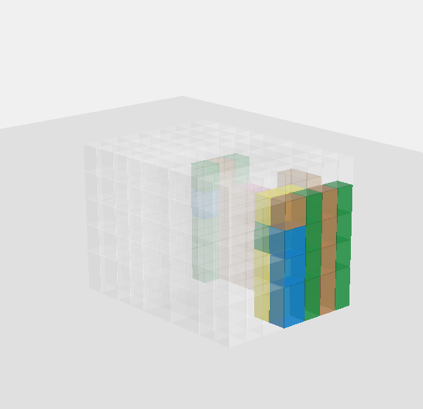
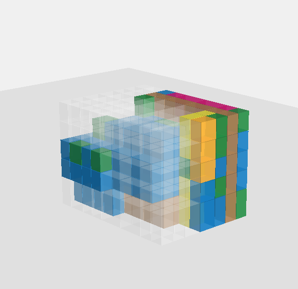
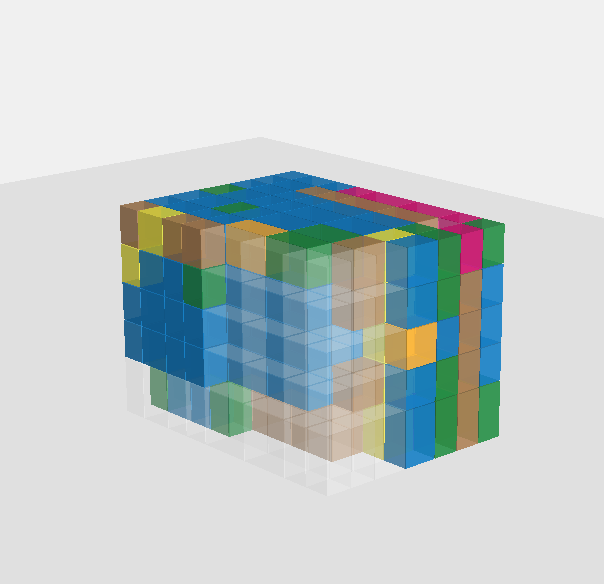
		(3)

Figure 16: Reconstruction: design reconstruction of sample sequences from the evaluation data and comparison with the ground truth.

.

		Ground Truth
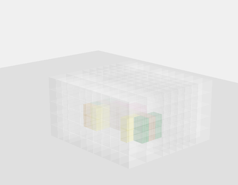
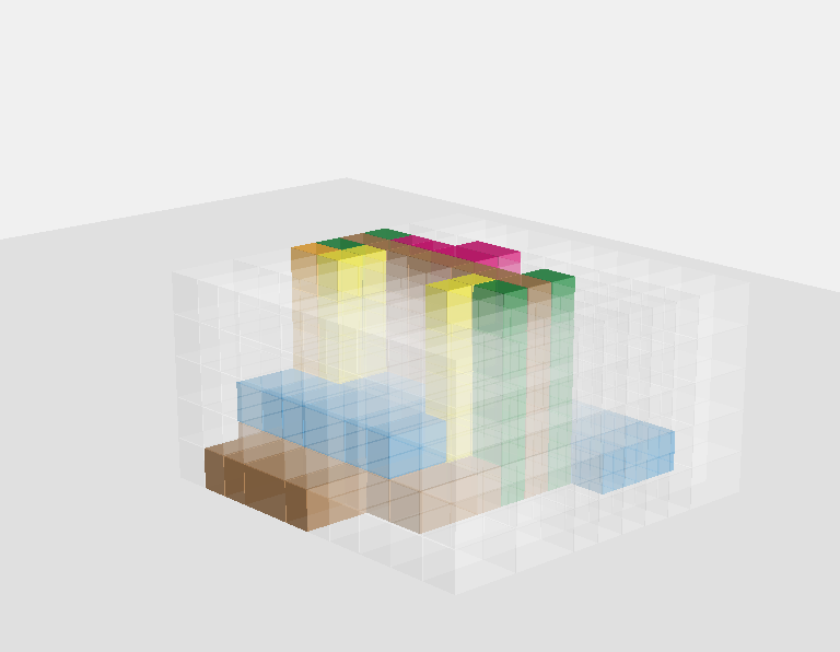
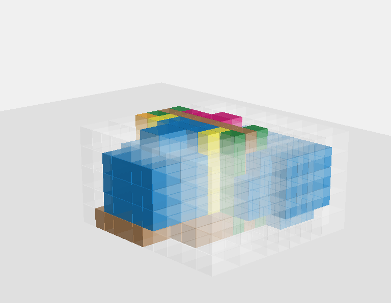
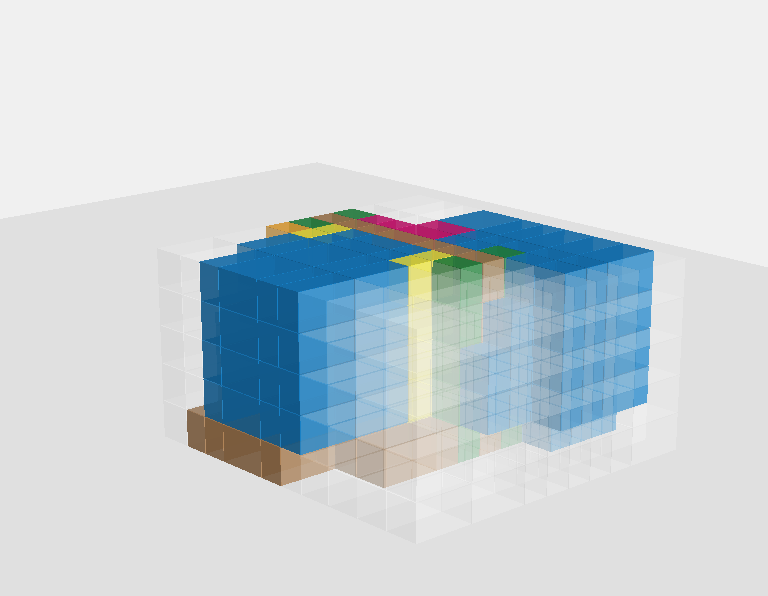
		Autocompletion
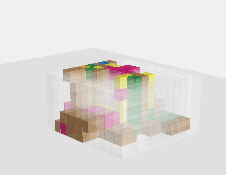
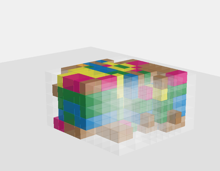
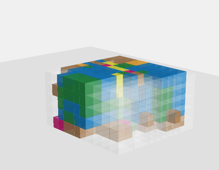
		(1)
		Ground Truth
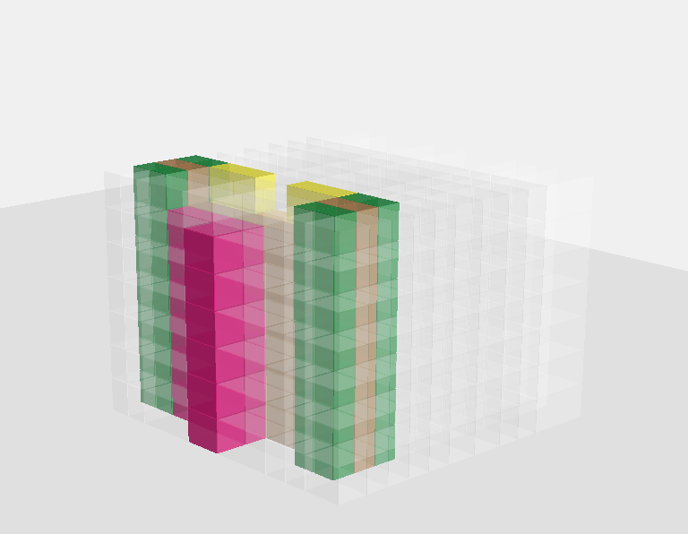
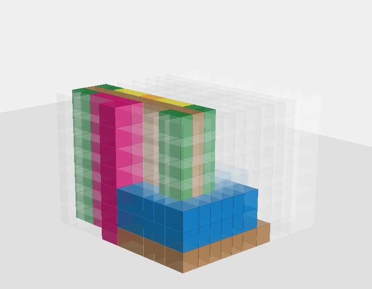
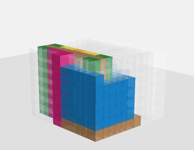
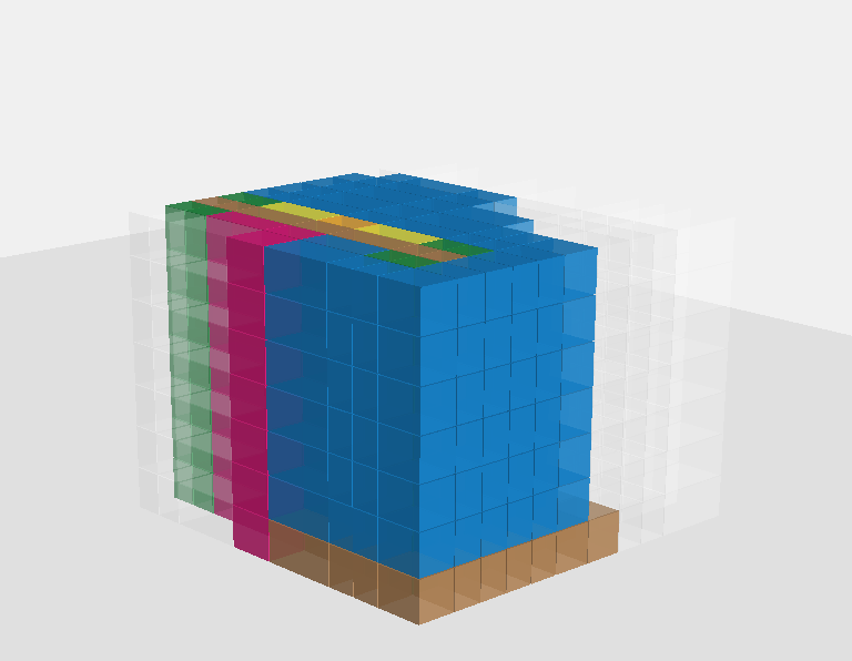
		Autocompletion
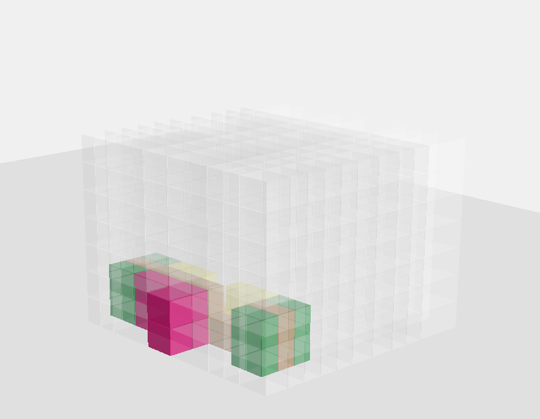
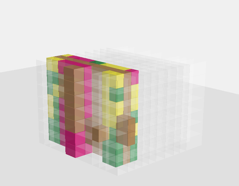
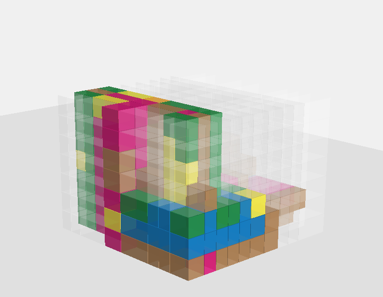
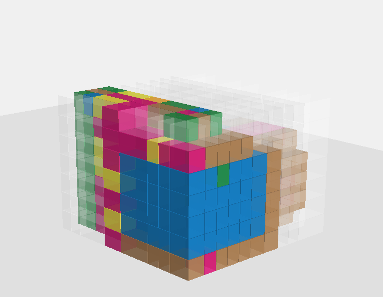
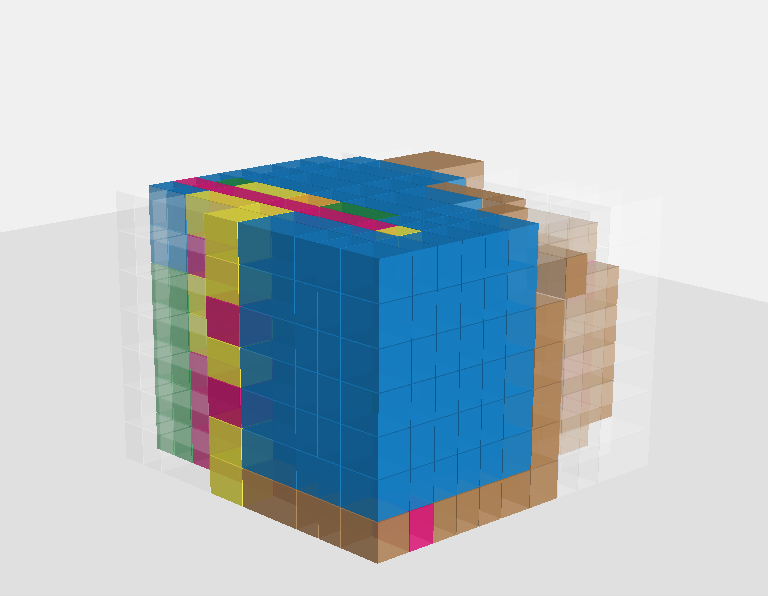
		(2)
		Ground Truth
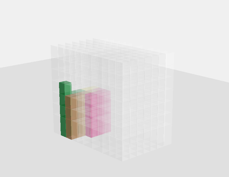
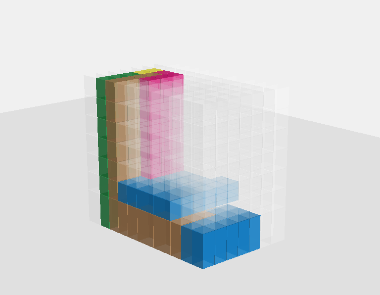
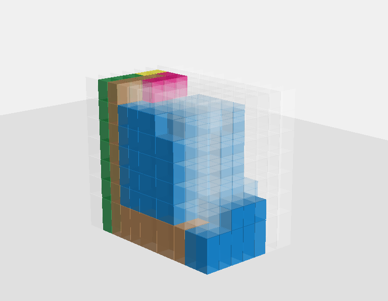
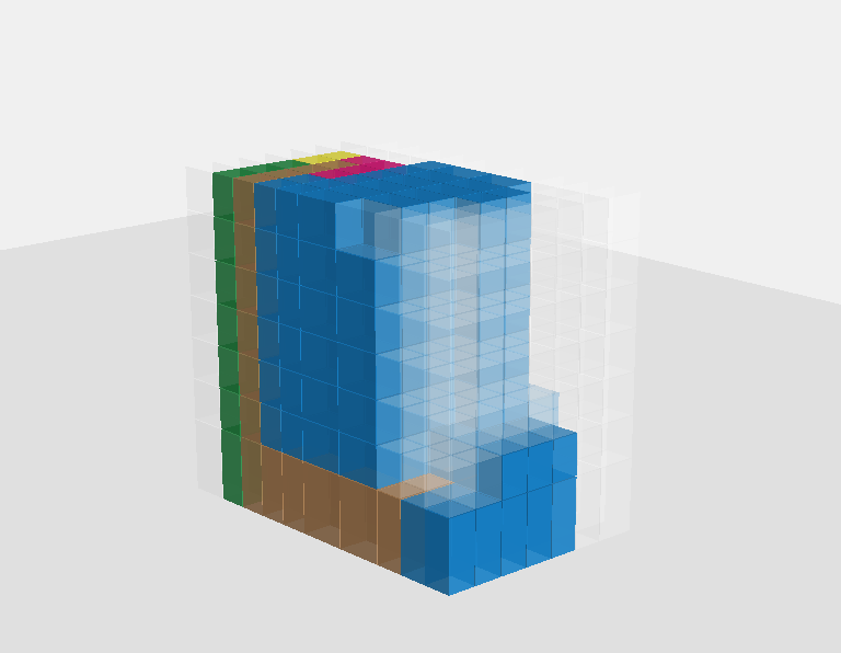
		Autocompletion
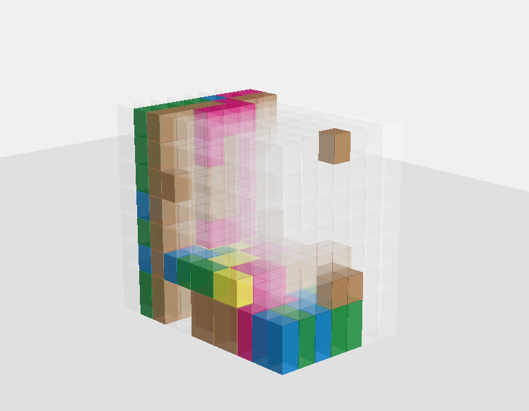
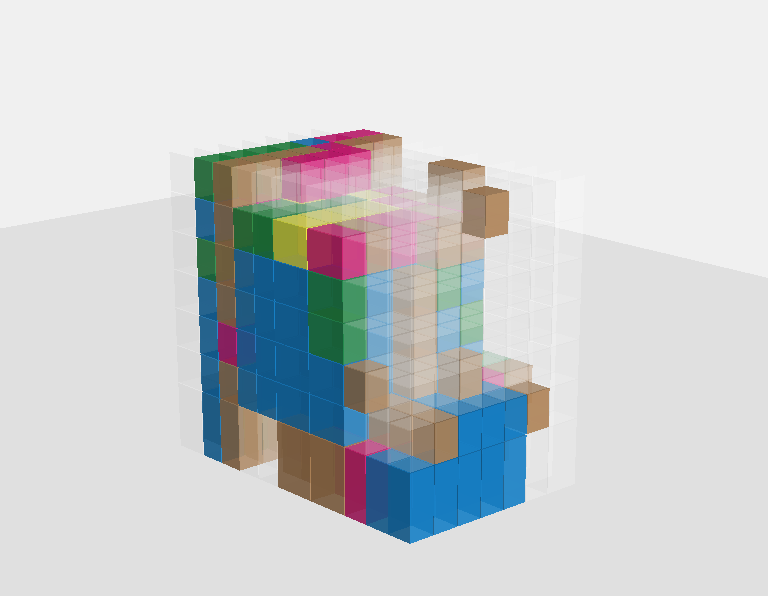
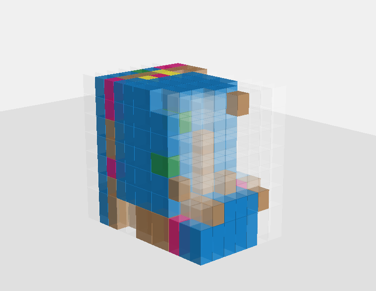
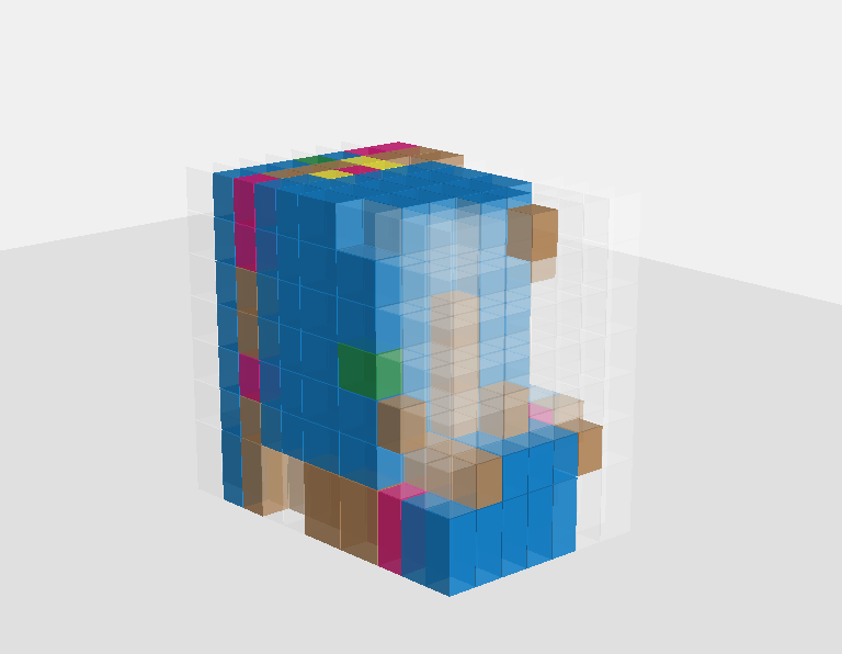
		(3)

Figure 17: Autocompletion: design autocompletion from a partial design given at t=0 from the training data and comparison with the ground truth.

.

		Ground Truth
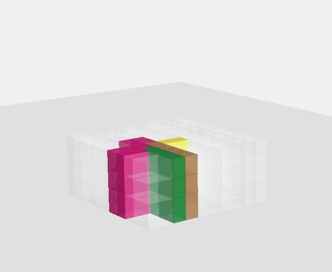
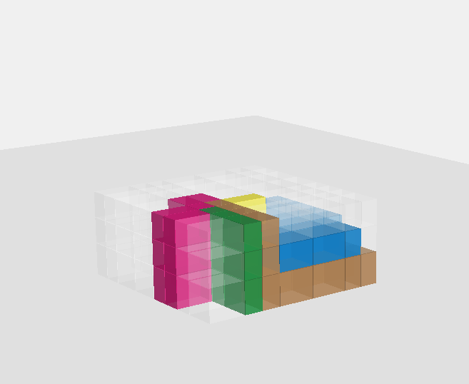
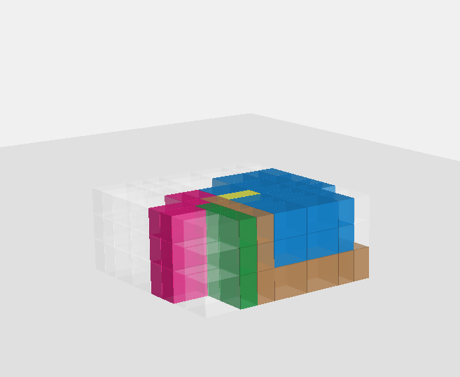
		Autocompletion
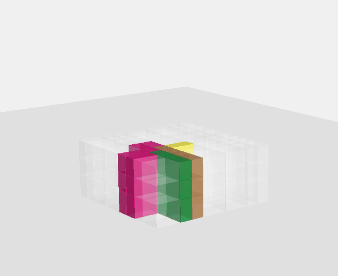
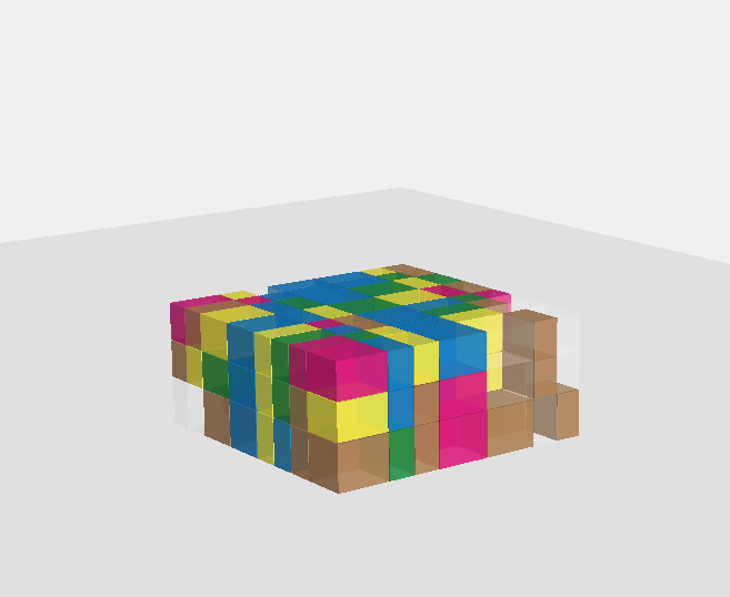
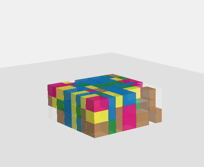
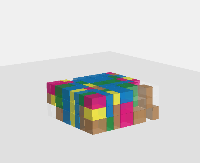
		(1)
		Ground Truth
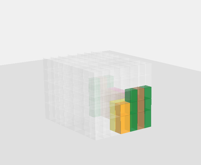
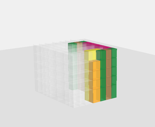
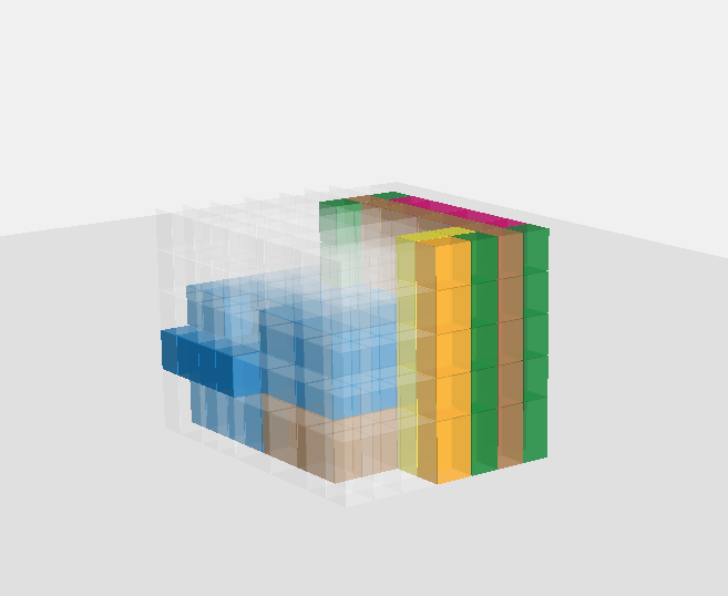
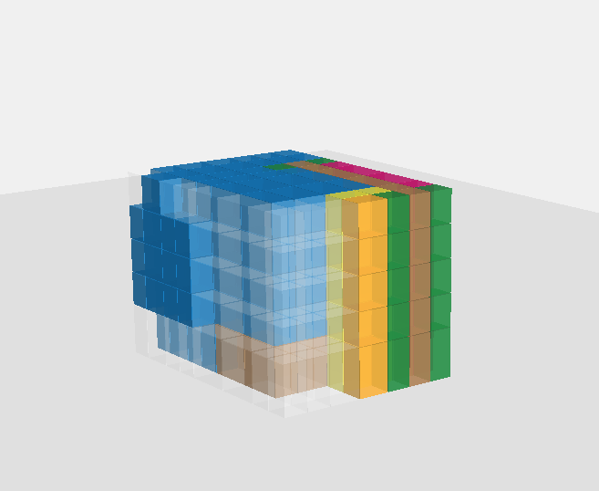
		Autocompletion
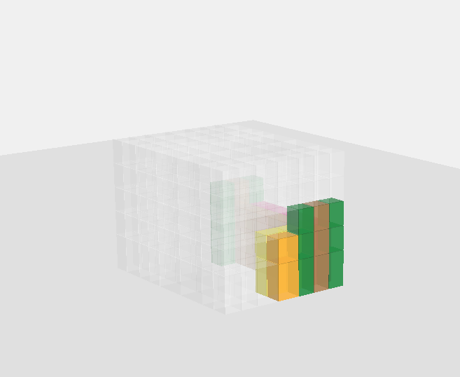
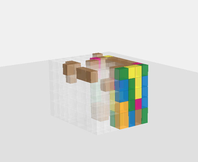
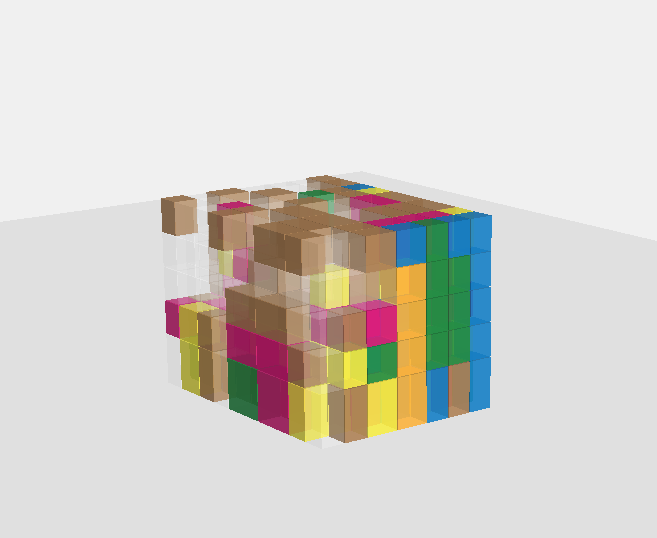
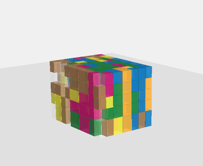
		Ground Truth
		(2)
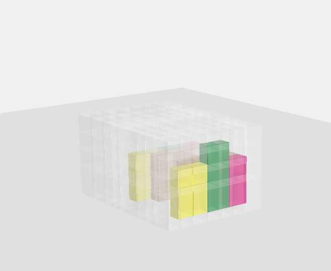
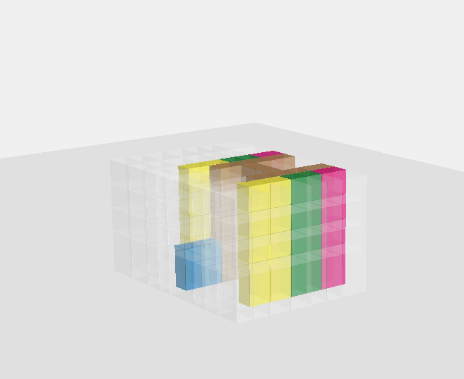
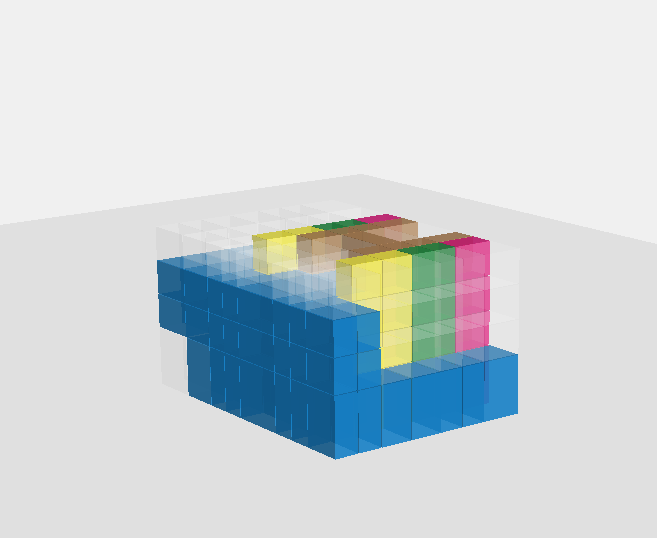
		Autocompletion
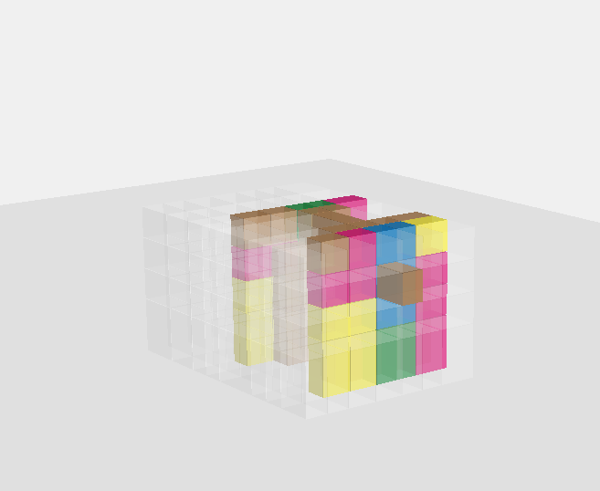
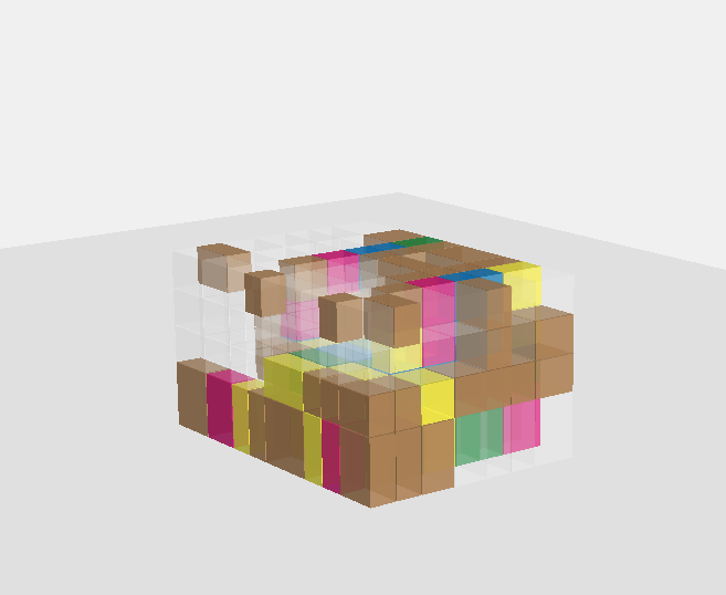
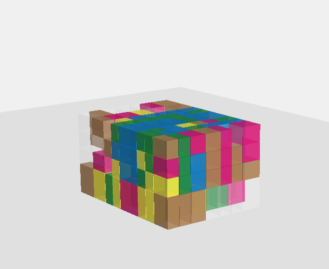
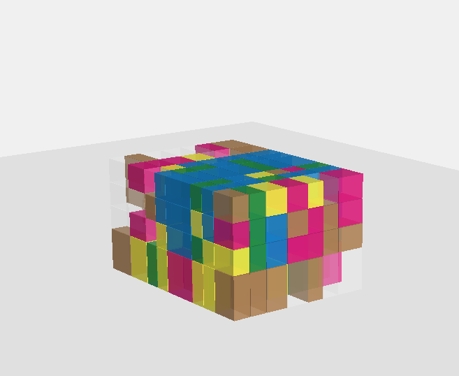
		(3)

Figure 18: Autocompletion: design autocompletion from a partial design given at t=0 from the evaluation data and comparison with the ground truth.

.

		H = 0
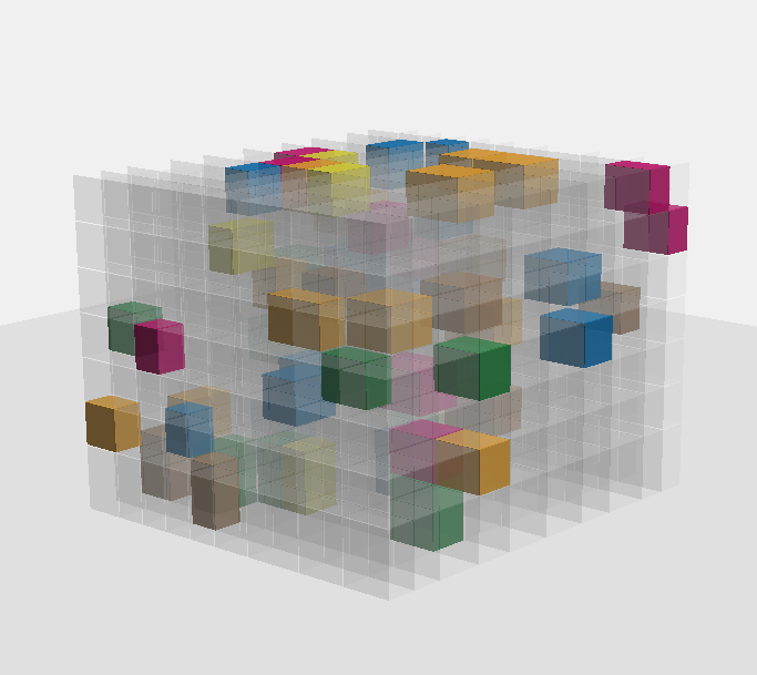
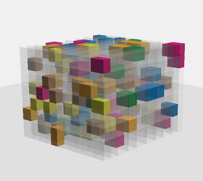
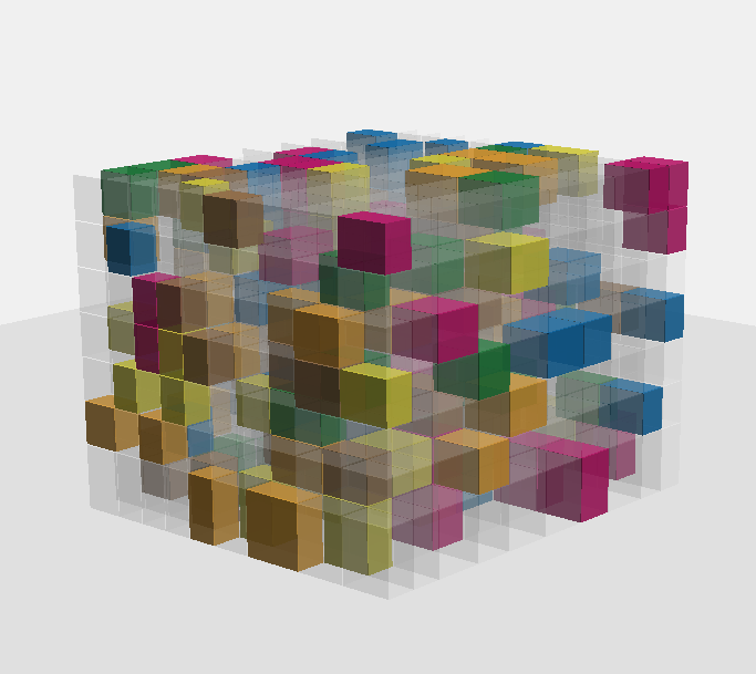
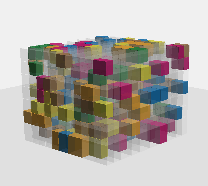
		H = 100
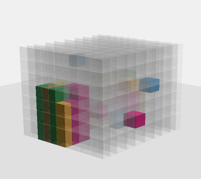
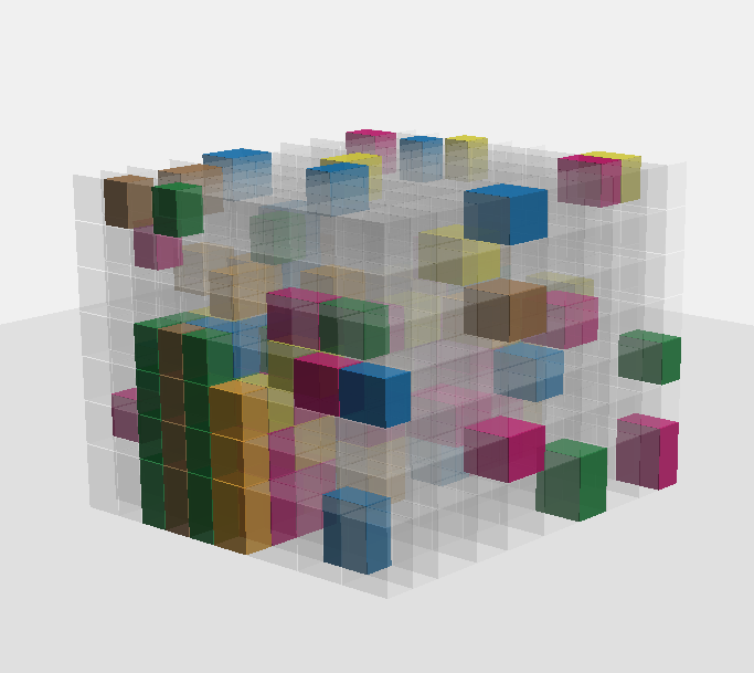
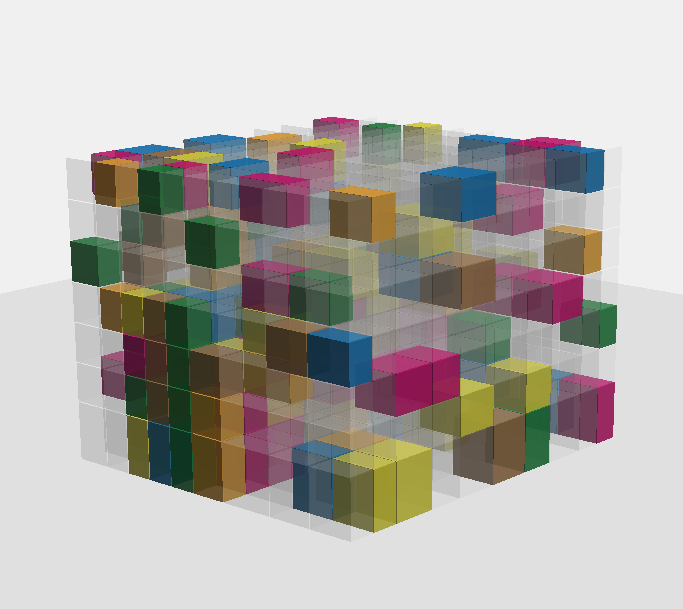
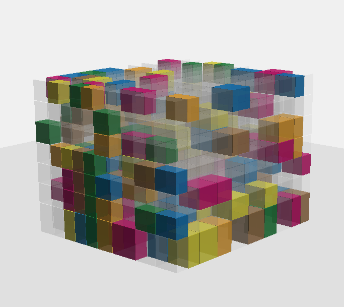
		H = 200
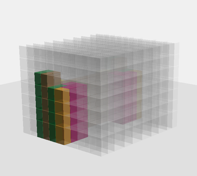
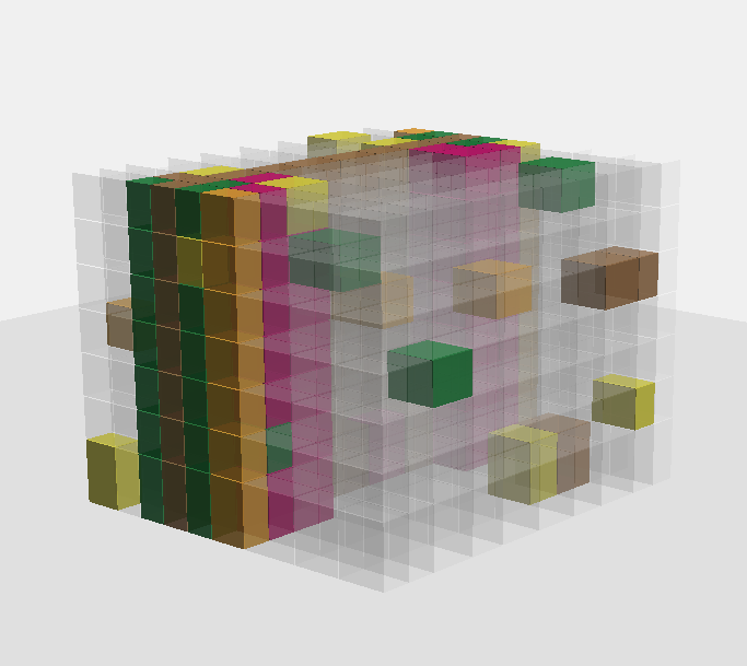
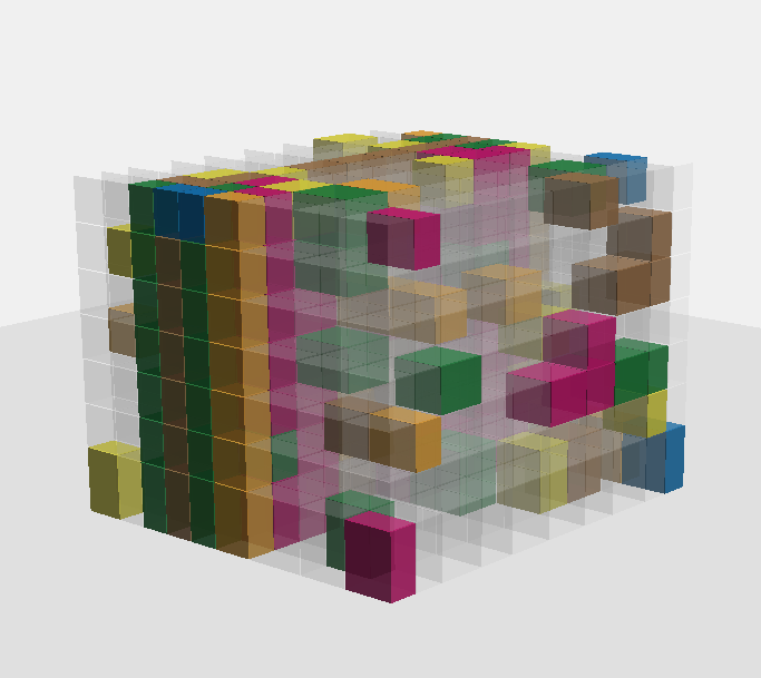
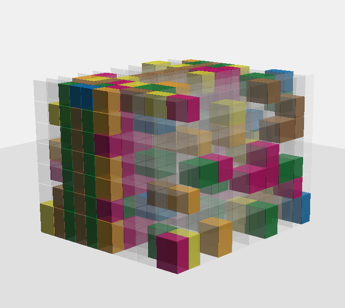
		H = 300
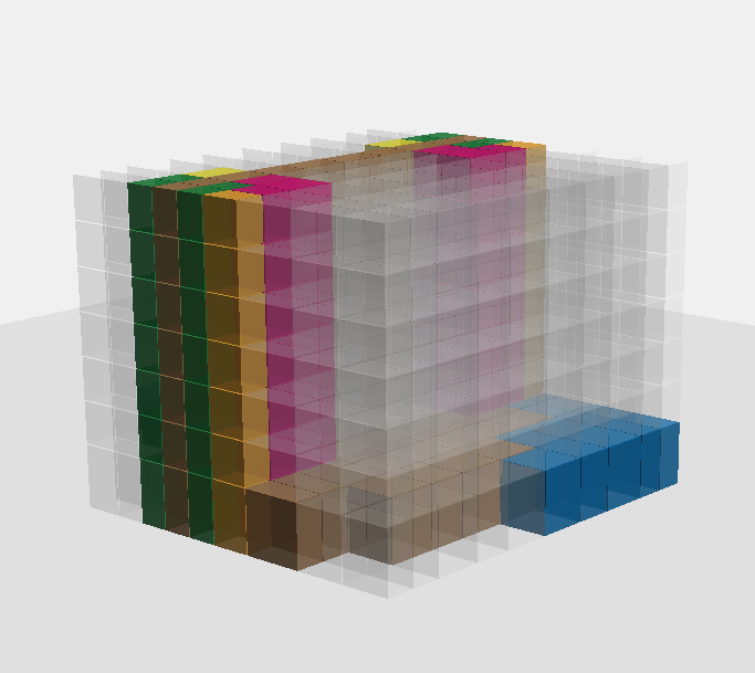
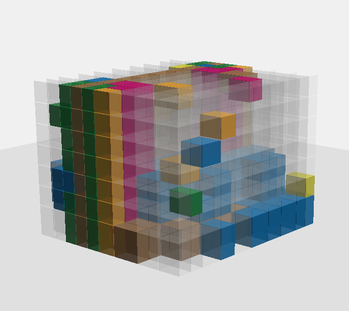
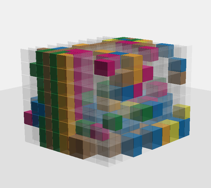
		H = 400
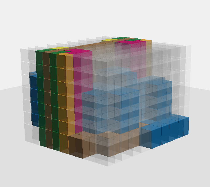
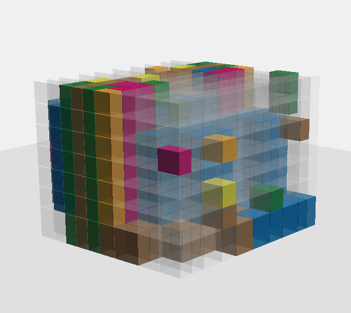
		Ground truth
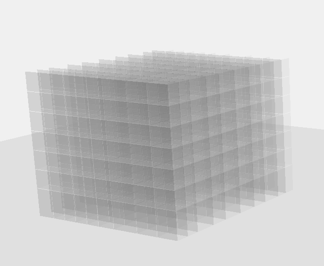
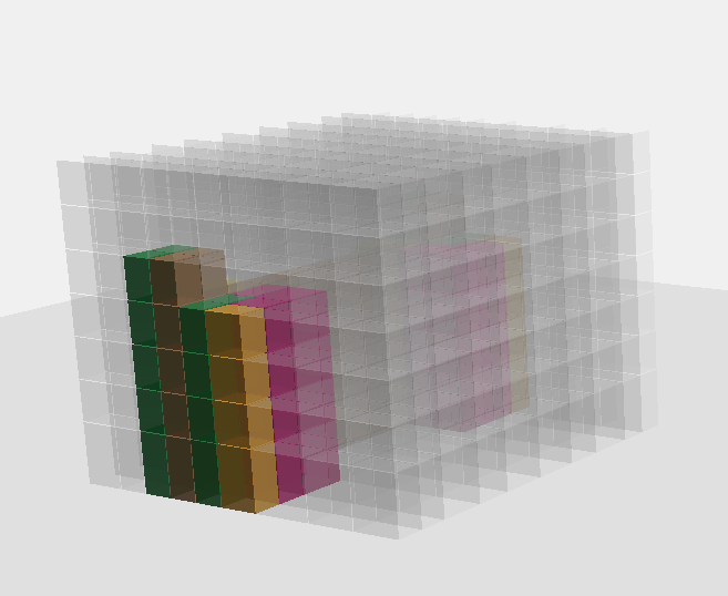
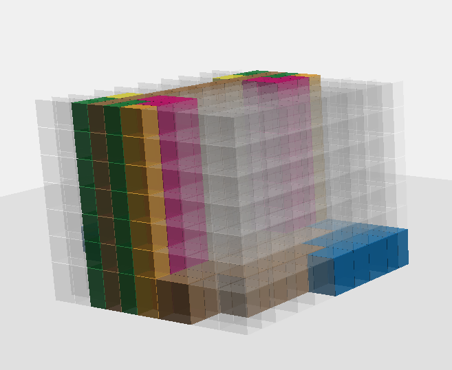
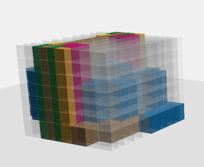
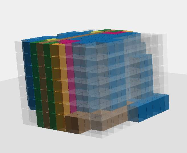
(a) t = 0	(b) t = 12	(c) t = 24	(d) t = 36	(e) t = 45

Figure 19: An example sequence created from five different degrees of randomnesses of the evaluation data; a) $H=0$ means randomly generated sequence, b) $H=100$ means optimal policy being followed after 100 timesteps, c) b) $H=200$ means optimal policy being followed after 200 timesteps, d) $H=300$ means optimal policy being followed after 300 timesteps, e) $H=400$ means optimal policy being followed after 400 timesteps,

.

References

- [1] Max Bain, Arsha Nagrani, Gül Varol, and Andrew Zisserman. Frozen in time: A joint video and image encoder for end-to-end retrieval. In Proceedings of the IEEE/CVF International Conference on Computer Vision, pages 1728–1738, 2021.
- [2] Hangbo Bao, Li Dong, Songhao Piao, and Furu Wei. Beit: Bert pre-training of image transformers. arXiv preprint arXiv:2106.08254, 2021.
- [3] Greg Brockman, Vicki Cheung, Ludwig Pettersson, Jonas Schneider, John Schulman, Jie Tang, and Wojciech Zaremba. Openai gym. arXiv preprint arXiv:1606.01540, 2016.
- [4] Tom Brown, Benjamin Mann, Nick Ryder, Melanie Subbiah, Jared D Kaplan, Prafulla Dhariwal, Arvind Neelakantan, Pranav Shyam, Girish Sastry, Amanda Askell, et al. Language models are few-shot learners. Advances in neural information processing systems, 33:1877–1901, 2020.
- [5] Kai-Hung Chang, Chin-Yi Cheng, Jieliang Luo, Shingo Murata, Mehdi Nourbakhsh, and Yoshito Tsuji. Building-gan: Graph-conditioned architectural volumetric design generation. In Proceedings of the IEEE/CVF International Conference on Computer Vision, pages 11956–11965, 2021.
- [6] Jiacheng Chen, Yiming Qian, and Yasutaka Furukawa. Heat: Holistic edge attention transformer for structured reconstruction. In Proceedings of the IEEE/CVF Conference on Computer Vision and Pattern Recognition, pages 3866–3875, 2022.
- [7] Jacob Devlin, Ming-Wei Chang, Kenton Lee, and Kristina Toutanova. Bert: Pre-training of deep bidirectional transformers for language understanding. arXiv preprint arXiv:1810.04805, 2018.
- [8] Xinhan Di, Pengqian Yu, Danfeng Yang, Hong Zhu, Changyu Sun, and YinDong Liu. End-to-end generative floor-plan and layout with attributes and relation graph. arXiv preprint arXiv:2012.08514, 2020.
- [9] Laurent Dinh, Jascha Sohl-Dickstein, and Samy Bengio. Density estimation using real nvp. arXiv preprint arXiv:1605.08803, 2016.
- [10] Mathieu Germain, Karol Gregor, Iain Murray, and Hugo Larochelle. Made: Masked autoencoder for distribution estimation. In International conference on machine learning, pages 881–889. PMLR, 2015.
- [11] Edoardo Giacomello, Pier Luca Lanzi, and Daniele Loiacono. Searching the latent space of a generative adversarial network to generate doom levels. In 2019 IEEE Conference on Games (CoG), pages 1–8. IEEE, 2019.
- [12] Zhaohan Daniel Guo, Bernardo Avila Pires, Bilal Piot, Jean-Bastien Grill, Florent Altché, Rémi Munos, and Mohammad Gheshlaghi Azar. Bootstrap latent-predictive representations for multitask reinforcement learning. In International Conference on Machine Learning, pages 3875–3886. PMLR, 2020.
- [13] Chenhang He, Ruihuang Li, Shuai Li, and Lei Zhang. Voxel set transformer: A set-to-set approach to 3d object detection from point clouds. In Proceedings of the IEEE/CVF Conference on Computer Vision and Pattern Recognition, pages 8417–8427, 2022.
- [14] Kaiming He, Xinlei Chen, Saining Xie, Yanghao Li, Piotr Dollár, and Ross Girshick. Masked autoencoders are scalable vision learners. In Proceedings of the IEEE/CVF Conference on Computer Vision and Pattern Recognition, pages 16000–16009, 2022.
- [15] Martin Heusel, Hubert Ramsauer, Thomas Unterthiner, Bernhard Nessler, and Sepp Hochreiter. Gans trained by a two time-scale update rule converge to a local nash equilibrium. Advances in neural information processing systems, 30, 2017.
- [16] Max Jaderberg, Volodymyr Mnih, Wojciech Marian Czarnecki, Tom Schaul, Joel Z Leibo, David Silver, and Koray Kavukcuoglu. Reinforcement learning with unsupervised auxiliary tasks. arXiv preprint arXiv:1611.05397, 2016.
- [17] Benjamin T Jones, Michael Hu, Vladimir G Kim, and Adriana Schulz. Self-supervised representation learning for cad. arXiv preprint arXiv:2210.10807, 2022.
- [18] Diederik P Kingma and Max Welling. Auto-encoding variational bayes. arXiv preprint arXiv:1312.6114, 2013.
- [19] Joseph G. Lambourne, Karl D.D. Willis, Pradeep Kumar Jayaraman, Aditya Sanghi, Peter Meltzer, and Hooman Shayani. Brepnet: A topological message passing system for solid models. In Proceedings of the IEEE/CVF Conference on Computer Vision and Pattern Recognition (CVPR), pages 12773–12782, June 2021.
- [20] Jie Lei, Linjie Li, Luowei Zhou, Zhe Gan, Tamara L Berg, Mohit Bansal, and Jingjing Liu. Less is more: Clipbert for video-and-language learning via sparse sampling. In Proceedings of the IEEE/CVF Conference on Computer Vision and Pattern Recognition, pages 7331–7341, 2021.
- [21] Changjian Li, Hao Pan, Adrien Bousseau, and Niloy J. Mitra. Sketch2cad: Sequential cad modeling by sketching in context. ACM Trans. Graph. (Proceedings of SIGGRAPH Asia 2020), 39(6):164:1–164:14, 2020.
- [22] Huaishao Luo, Lei Ji, Ming Zhong, Yang Chen, Wen Lei, Nan Duan, and Tianrui Li. Clip4clip: An empirical study of clip for end to end video clip retrieval and captioning. Neurocomputing, 508:293–304, 2022.
- [23] Jiageng Mao, Minzhe Niu, Chenhan Jiang, Hanxue Liang, Jingheng Chen, Xiaodan Liang, Yamin Li, Chaoqiang Ye, Wei Zhang, Zhenguo Li, et al. One million scenes for autonomous driving: Once dataset. arXiv preprint arXiv:2106.11037, 2021.
- [24] Jiageng Mao, Yujing Xue, Minzhe Niu, Haoyue Bai, Jiashi Feng, Xiaodan Liang, Hang Xu, and Chunjing Xu. Voxel transformer for 3d object detection. In Proceedings of the IEEE/CVF International Conference on Computer Vision, pages 3164–3173, 2021.
- [25] Nelson Nauata, Kai-Hung Chang, Chin-Yi Cheng, Greg Mori, and Yasutaka Furukawa. House-gan: Relational generative adversarial networks for graph-constrained house layout generation. In Computer Vision–ECCV 2020: 16th European Conference, Glasgow, UK, August 23–28, 2020, Proceedings, Part I 16, pages 162–177. Springer, 2020.
- [26] Akshay Gadi Patil, Manyi Li, Matthew Fisher, Manolis Savva, and Hao Zhang. Layoutgmn: Neural graph matching for structural layout similarity. In Proceedings of the IEEE/CVF Conference on Computer Vision and Pattern Recognition, pages 11048–11057, 2021.
- [27] Jesús Andrés Portillo-Quintero, José Carlos Ortiz-Bayliss, and Hugo Terashima-Marín. A straightforward framework for video retrieval using clip. In Pattern Recognition: 13th Mexican Conference, MCPR 2021, Mexico City, Mexico, June 23–26, 2021, Proceedings, pages 3–12. Springer, 2021.
- [28] Alec Radford, Jong Wook Kim, Chris Hallacy, Aditya Ramesh, Gabriel Goh, Sandhini Agarwal, Girish Sastry, Amanda Askell, Pamela Mishkin, Jack Clark, Gretchen Krueger, and Ilya Sutskever. Learning transferable visual models from natural language supervision. In Marina Meila and Tong Zhang, editors, Proceedings of the 38th International Conference on Machine Learning, volume 139 of Proceedings of Machine Learning Research, pages 8748–8763. PMLR, 18–24 Jul 2021.
- [29] Alec Radford, Jeffrey Wu, Rewon Child, David Luan, Dario Amodei, Ilya Sutskever, et al. Language models are unsupervised multitask learners. OpenAI blog, 1(8):9, 2019.
- [30] Aditya Sanghi, Hang Chu, Joseph G Lambourne, Ye Wang, Chin-Yi Cheng, Marco Fumero, and Kamal Rahimi Malekshan. Clip-forge: Towards zero-shot text-to-shape generation. In Proceedings of the IEEE/CVF Conference on Computer Vision and Pattern Recognition, pages 18603–18613, 2022.
- [31] Aditya Sanghi, Rao Fu, Vivian Liu, Karl Willis, Hooman Shayani, Amir Hosein Khasahmadi, Srinath Sridhar, and Daniel Ritchie. Textcraft: Zero-shot generation of high-fidelity and diverse shapes from text. arXiv preprint arXiv:2211.01427, 2022.
- [32] Mohammad Amin Shabani, Sepidehsadat Hosseini, and Yasutaka Furukawa. Housediffusion: Vector floorplan generation via a diffusion model with discrete and continuous denoising. arXiv preprint arXiv:2211.13287, 2022.
- [33] Abhishek Sharma, Oliver Grau, and Mario Fritz. Vconv-dae: Deep volumetric shape learning without object labels. In Computer Vision–ECCV 2016 Workshops: Amsterdam, The Netherlands, October 8-10 and 15-16, 2016, Proceedings, Part III 14, pages 236–250. Springer, 2016.
- [34] Evan Shelhamer, Parsa Mahmoudieh, Max Argus, and Trevor Darrell. Loss is its own reward: Self-supervision for reinforcement learning. arXiv preprint arXiv:1612.07307, 2016.
- [35] Ashish Vaswani, Noam Shazeer, Niki Parmar, Jakob Uszkoreit, Llion Jones, Aidan N Gomez, Łukasz Kaiser, and Illia Polosukhin. Attention is all you need. Advances in neural information processing systems, 30, 2017.
- [36] Karl DD Willis, Pradeep Kumar Jayaraman, Hang Chu, Yunsheng Tian, Yifei Li, Daniele Grandi, Aditya Sanghi, Linh Tran, Joseph G Lambourne, Armando Solar-Lezama, and Wojciech Matusik. Joinable: Learning bottom-up assembly of parametric cad joints. arXiv preprint arXiv:2111.12772, 2021.
- [37] Karl D. D. Willis, Yewen Pu, Jieliang Luo, Hang Chu, Tao Du, Joseph G. Lambourne, Armando Solar-Lezama, and Wojciech Matusik. Fusion 360 gallery: A dataset and environment for programmatic cad construction from human design sequences. ACM Transactions on Graphics (TOG), 40(4), 2021.
- [38] Jiajun Wu, Chengkai Zhang, Tianfan Xue, Bill Freeman, and Josh Tenenbaum. Learning a probabilistic latent space of object shapes via 3d generative-adversarial modeling. Advances in neural information processing systems, 29, 2016.
- [39] Yan Yan, Yuxing Mao, and Bo Li. Second: Sparsely embedded convolutional detection. Sensors, 18(10):3337, 2018.
- [40] Maosheng Ye, Shuangjie Xu, and Tongyi Cao. Hvnet: Hybrid voxel network for lidar based 3d object detection. In Proceedings of the IEEE/CVF conference on computer vision and pattern recognition, pages 1631–1640, 2020.
- [41] Tianwei Yin, Xingyi Zhou, and Philipp Krahenbuhl. Center-based 3d object detection and tracking. In Proceedings of the IEEE/CVF conference on computer vision and pattern recognition, pages 11784–11793, 2021.
- [42] Tao Yu, Zhizheng Zhang, Cuiling Lan, Zhibo Chen, and Yan Lu. Mask-based latent reconstruction for reinforcement learning. arXiv preprint arXiv:2201.12096, 2022.
- [43] Linqi Zhou, Yilun Du, and Jiajun Wu. 3d shape generation and completion through point-voxel diffusion. In Proceedings of the IEEE/CVF International Conference on Computer Vision, pages 5826–5835, 2021.
- [44] Yin Zhou and Oncel Tuzel. Voxelnet: End-to-end learning for point cloud based 3d object detection. In Proceedings of the IEEE conference on computer vision and pattern recognition, pages 4490–4499, 2018.
- [45] Jinhua Zhu, Yingce Xia, Lijun Wu, Jiajun Deng, Wengang Zhou, Tao Qin, Tie-Yan Liu, and Houqiang Li. Masked contrastive representation learning for reinforcement learning. IEEE Transactions on Pattern Analysis and Machine Intelligence, 2022.