The Robust F-Statistic as a Test for Weak Instruments

Abstract

Montiel Olea and Pflueger (2013) proposed the effective F-statistic as a test for weak instruments in terms of the Nagar bias of the two-stage least squares (2SLS) estimator relative to a benchmark worst-case bias. We show that their methodology applies to a class of linear generalized method of moments (GMM) estimators with an associated class of generalized effective F-statistics. The standard nonhomoskedasticity robust F-statistic is a member of this class. The associated GMMf estimator, with the extension “f” for first-stage, is a novel and unusual estimator as the weight matrix is based on the first-stage residuals. As the robust F-statistic can also be used as a test for underidentification, expressions for the calculation of the weak-instruments critical values in terms of the Nagar bias of the GMMf estimator relative to the benchmark simplify and no simulation methods or Patnaik (1949) distributional approximations are needed. In the grouped-data IV designs of Andrews (2018), where the robust F-statistic is large but the effective F-statistic is small, the GMMf estimator is shown to behave much better in terms of bias than the 2SLS estimator, as expected by the weak-instruments test results.

Keywords: Instrumental variables, weak instruments, nonhomoskedasticity, robust F-statistic, GMM

JEL Codes: C12, C26

1 Introduction

It is commonplace to report the first-stage F-statistic to test for weak instruments in linear models with a single endogenous variable, estimated by two-stage least squares (2SLS). This follows the work of Staiger and Stock (1997) and Stock and Yogo (2005), with the latter providing critical values for the first-stage non-robust F-statistic for null hypotheses of weak instruments in terms of bias of the 2SLS estimator relative to that of the OLS estimator and Wald-test size distortions. These weak-instruments critical values for the non-robust F-statistic are valid only under homoskedasticity (i.e. conditional homoskedasticity, no serial correlation and no clustering) of both the first-stage and structural errors, and do not apply to the robust (to nonhomoskedasticity) F-statistic in general designs, see Bun and de Haan (2010), Montiel Olea and Pflueger (2013) and Andrews (2018). In particular, Andrews (2018) found for some cross-sectional heteroskedastic designs that the standard 2SLS confidence intervals had large coverage distortions even for very large values of the robust F-statistic. For example, he found for a high endogeneity design that “the 2SLS confidence set has a 15% coverage distortion even when the mean of the first-stage robust F-statistic is 100,000”, Andrews (2018, Supplementary Appendix, p 11).

For general nonhomoskedasticity, Montiel Olea and Pflueger (2013) proposed the first-stage effective F-statistic and derived critical values for the null of weak instruments in terms of the Nagar bias of the 2SLS estimator, relative to a benchmark worst-case bias. As shown in Section 4.3.1, the effective F-statistics in the designs of Andrews (2018) do not reject the null of weak instruments, and therefore correctly indicate the poor performance of the 2SLS estimator. In their review paper Andrews, Stock, and Sun (2019, p 729) recommend “that researchers judge instrument strength based on the effective F-statistic of Montiel Olea and Pflueger (2013)”.

The effective F-statistic is specific to the Nagar bias of the 2SLS estimator and the main contribution of this paper is that the methods of Montiel Olea and Pflueger (2013) apply to a wider class of linear generalized method of moments (GMM) estimators resulting in a class of associated generalized effective F-statistics. The nonhomoskedasticity robust F-statistic is a member of this class, and we call its associated GMM estimator the GMMf estimator, with the extension “f” for first-stage. This is because the weight matrix of the GMMf estimator is based on the first-stage residuals, with $k_{z}$ times the robust F-statistic being the denominator of the GMMf estimator, where $k_{z}$ is the number of excluded instruments. This is similar to the relationship of the non-robust F-statistic and the 2SLS estimator.

Unlike the effective F-statistic, the robust F-statistic can be used for testing $H_{0}:\pi=0$, where $\pi$ is the vector of parameters on the excluded instruments in the first-stage linear model specification. Under the null, its limiting distribution is central chi-square, scaled by the degrees of freedom, $k_{z}$. Under the alternative, its limiting distribution is non-central chi-square. The methods needed for calculating the critical values for the null of weak instruments in terms of the Nagar bias of the GMMf estimator relative to its benchmark worst-case bias are simpler for the robust F-statistic than for the effective F-statistic. For the robust F-statistic no simulation methods or Patnaik (1949) curve-fitting approximation is needed. In that sense, the relationship between the robust F-statistic and the GMMf estimator can be described as being canonical.

Section 2 introduces the linear model specification, main assumptions, effective and robust F-statistics and the GMMf estimator. Section 3 then formulates the class of generalized F-statistics for the class of linear GMM estimators and shows that the weak-instruments testing methods developed by Montiel Olea and Pflueger (2013) apply straightforwardly to this class. The section then provides a summary of the Montiel Olea and Pflueger (2013) results. Section 4 shows how the general results and specifications simplify for the robust-F statistic in relation to the Nagar bias of the GMMf estimator. As the Nagar bias is relative to a benchmark worse-case bias, which is estimator specific, we harmonize in Section 4.1 the benchmark bias by considering the worst-case OLS bias as the benchmark, which applies to the class of GMM estimators considered.

When the value of the robust F-statistic is large in the Andrews (2018) designs, this then implies that the GMMf estimator does not suffer from a weak-instruments problem, which is indeed confirmed in Section 4.3.1, where we replicate the Monte Carlo analysis of Andrews (2018). The design is the same as a grouped-data one, see Angrist (1991) and the discussion in Angrist and Pischke (2009), where the instruments are mutually exclusive group membership indicators. In the two designs considered, there is in each only one informative group, but the first-stage heteroskedasticity is such that the 2SLS estimator does not utilize this information well, whereas the GMMf estimator gives almost all the weight to the informative groups.

The advice for practice is then to report both the effective and robust F-statistics, together with their critical values, and to consider the GMMf estimator in cases where there is a clear discrepancy with a large value for the robust F-statistic. We do this in Section 5 for specifications of Stephens and Yang (2014), who study the effect of schooling on wages using data from the 1960-1980 US Censuses of Population. The endogenous variable is years of schooling and the instruments are three indicator variables corresponding to being required to attend seven, eight or nine or more years of schooling. The specifications are estimated by 2SLS and Stephens and Yang (2014) report the robust F-statistic but not the effective F-statistic. We find no large discrepancies between the two measures, and the GMMf estimates are very similar to the 2SLS ones. We give some concluding remarks in Section 6.

2 Model, Assumptions and F-Statistics

We have a sample $\left\{y_{i},x_{i},z_{i}\right\}_{i=1}^{n}$, where $z_{i}$ is a $k_{z}$-vector of instrumental variables. We are interested in the effect of $x$ on $y$ in a linear model specification, where $x$ is endogenously determined. We consider the linear structural and first-stage specifications

$$y =x\beta+u$$ (1)

$$x =Z\pi+v_{2},$$ (2)

where $y$, $x$, $u$ and $v_{2}$ are $n$-vectors and $Z$ an $n\times k_{z}$ matrix. Other exogenous explanatory variables, including the constant have been partialled out. The reduced-form specification for $y$ is then given by

$$y=Z\pi\beta+v_{1}=Z\pi_{y}+v_{1},$$ (3)

where $v_{1}=u+\beta v_{2}$, and $\pi_{y}=\pi\beta$.

Following Montiel Olea and Pflueger (2013), we make the following assumptions.

Assumption 1.

1. Weak instruments asymptotics. The vector $\pi$ is local to zero,

   $$\pi=\pi_{n}=c/\sqrt{n},$$

   where $c$ is a fixed vector $c\in\mathbb{R}^{k_{z}}$.

2. As $n\rightarrow\infty$,

   $$\frac{1}{n}Z^{\prime}Z \overset{p}{\rightarrow}Q_{zz};$$

   $$\frac{1}{n}\left[v_{1}\,v_{2}\right]^{\prime}\left[v_{1}\,v_{2}\right] \stackrel{{\scriptstyle p}}{{\rightarrow}}\Sigma_{v};$$

   $$\frac{1}{\sqrt{n}}\left(\begin{array}[]{c}Z^{\prime}v_{1}\\ Z^{\prime}v_{2}\end{array}\right) \overset{d}{\rightarrow}\left(\begin{array}[]{c}\psi_{1}\\ \psi_{2}\end{array}\right)\sim N\left(0,W\right),$$

   with $Q_{zz}$, $\Sigma_{v}$ and $W$ finite, positive definite matrices, and

   $$\Sigma_{v} =\left[\begin{array}[]{cc}\sigma_{1}^{2}&\sigma_{12}\\ \sigma_{12}&\sigma_{2}^{2}\end{array}\right];$$

   $$W =\left[\begin{array}[]{cc}W_{1}&W_{12}\\ W_{12}^{\prime}&W_{2}\end{array}\right].$$

3. There exists a sequence of positive definite estimates $\left\{\widehat{W}_{n}\right\}$, such that $\widehat{W}_{n}\overset{p}{\rightarrow}W$ as $n\rightarrow\infty$.

In the remainder, we drop the subscript $n$ from $\widehat{W}_{n}$ for ease of exposition, and, commensurate with the partitioning of $W$,

$$\widehat{W}=\left[\begin{array}[]{cc}\widehat{W}_{1}&\widehat{W}_{12}\\ \widehat{W}_{12}^{\prime}&\widehat{W}_{2}\end{array}\right].$$

The two-stage least squares (2SLS) estimator is given by

$$\widehat{\beta}_{2sls}=\frac{x^{\prime}P_{Z}y}{x^{\prime}P_{Z}x},$$

where $P_{Z}=Z\left(Z^{\prime}Z\right)^{-1}Z^{\prime}$. The standard nonrobust first-stage F-statistic is

$$\widehat{F}=\frac{x^{\prime}P_{Z}x}{k_{z}\widehat{\sigma}_{v_{2}}^{2}},$$

where $\widehat{\sigma}_{v_{2}}^{2}=\widehat{v}_{2}^{\prime}\widehat{v}_{2}/n$, $\widehat{v}_{2}=\left(I_{n}-P_{Z}\right)x$, where $I_{n}$ is the identity matrix of order $n$. Note that we refrain throughout from finite sample degrees-of-freedom corrections in the exposition. It follows that we can alternatively express the 2SLS estimator as

$$\widehat{\beta}_{2sls}=\frac{\widehat{\pi}^{\prime}\left(V\widehat{a}r\left(\widehat{\pi}\right)\right)^{-1}\widehat{\pi}_{y}}{\widehat{\pi}^{\prime}\left(V\widehat{a}r\left(\widehat{\pi}\right)\right)^{-1}\widehat{\pi}}=\frac{\widehat{\pi}^{\prime}\left(V\widehat{a}r\left(\widehat{\pi}\right)\right)^{-1}\widehat{\pi}_{y}}{k_{z}\widehat{F}},$$ (4)

where $\widehat{\pi}$ and $\widehat{\pi}_{y}$ are the OLS estimators of $\pi$ and $\pi_{y}$ in the first-stage and reduced-form models (2) and (3), and $V\widehat{a}r\left(\widehat{\pi}\right)=\widehat{\sigma}_{v_{2}}^{2}\left(Z^{\prime}Z\right)^{-1}$, the non-robust estimator of the variance of $\widehat{\pi}$.

$\widehat{F}$ can be used as a test for weak instruments in terms of the bias of the 2SLS estimator relative to that of the OLS estimator of $\beta$, or the size distortion of the Wald test for hypotheses on $\beta$, Stock and Yogo (2005). The Stock and Yogo critical values are valid only under conditional homoskedasticity of both $u$ and $v_{2}$, i.e. $\mathbb{E}\left[u_{i}|z_{i}\right]=\sigma_{u}^{2}$ and $\mathbb{E}\left[v_{2i}|z_{i}\right]=\sigma_{v_{2}}^{2}$, or $W=\Sigma_{v}\otimes Q_{zz}$, with $\Sigma_{v}=\mathbb{E}\left[v_{i}v_{i}^{\prime}\right]$ and $v_{i}=\left(v_{1i},v_{2i}\right)^{\prime}$.

The nonhomoskedasticity-robust F-statistic is given by

$$\widehat{F}_{r}=\frac{x^{\prime}Z\widehat{W}_{2}^{-1}Z^{\prime}x}{nk_{z}}$$

and is a standard test statistic for testing $H_{0}:\pi=0$ under general forms of nonhomoskedasticity. But $\widehat{F}_{r}$ cannot be used as a test for weak instruments in relation to the behaviour of the 2SLS estimator. Andrews (2018) showed in a grouped-data IV design that $\widehat{F}_{r}$ could take very large values, of the order of $100,000$, whereas the 2SLS estimator was still poorly behaved in terms of bias and Wald test size.

For the 2SLS estimator, Montiel Olea and Pflueger (2013) proposed the effective F-statistic

$$\widehat{F}_{\text{eff}} =\frac{x^{\prime}P_{Z}x}{\text{tr}\left(\left(\frac{1}{n}Z^{\prime}Z\right)^{-1/2}\widehat{W}_{2}\left(\frac{1}{n}Z^{\prime}Z\right)^{-1/2}\right)}$$

$$=\frac{x^{\prime}P_{Z}x}{\text{tr}\left(\widehat{W}_{2}\left(\frac{1}{n}Z^{\prime}Z\right)^{-1}\right)}$$

and showed that this F-statistic can be used as a test for weak instruments in relation to the Nagar (1959) bias of the 2SLS estimator, relative to a worst-case benchmark. Andrews et al. (2019) advocate the use of $\widehat{F}_{\text{eff}}$ to gauge instrument strength for the 2SLS estimator. Although this weak-instrument test is related to the bias, the results presented in Andrews et al. (2019, Section 3) for a sample of 106 specifications from papers published in the American Economic Review suggest that the effective F-statistic “may convey useful information about the instrument strength more broadly, since we see that conventional asymptotic approximations appear reasonable in specifications where the effective F-statistic exceeds 10.”, Andrews et al. (2019, p 739).

In the next section, we introduce a class of generalized effective F-statistics, denoted $\widehat{F}_{\text{geff}}$, associated with a class of linear Generalized Method of Moments (GMM) estimators. We show that the weak-instrument Nagar bias results of Montiel Olea and Pflueger (2013), derived for the effective F-statistic in relation to the 2SLS estimator, applies to this general class. The robust F-statistic is a member of this class and the associated GMM estimator, denoted GMMf, with the extension f for first stage, is defined as

$$\widehat{\beta}_{gmmf}=\frac{x^{\prime}Z\widehat{W}_{2}^{-1}Z^{\prime}y}{x^{\prime}Z\widehat{W}_{2}^{-1}Z^{\prime}x}.$$ (5)

This is a novel, and unusual GMM estimator, as the weight matrix is based on the first-stage residuals. As we will show and explain below, for the Andrews (2018) design with large values for the robust F-statistic, but small values for the effective F-statistic, this estimator is much better behaved in terms of bias and also inference than the 2SLS estimator.

Like the expression of the 2SLS estimator in (4), we can write the GMMf estimator as

$$\widehat{\beta}_{gmmf}=\frac{\widehat{\pi}^{\prime}\left(V\widehat{a}r_{r}\left(\widehat{\pi}\right)\right)^{-1}\widehat{\pi}_{y}}{\widehat{\pi}^{\prime}\left(V\widehat{a}r_{r}\left(\widehat{\pi}\right)\right)^{-1}\widehat{\pi}}=\frac{\widehat{\pi}^{\prime}\left(V\widehat{a}r_{r}\left(\widehat{\pi}\right)\right)^{-1}\widehat{\pi}_{y}}{k_{z}\widehat{F}_{r}},$$ (6)

where $V\widehat{a}r_{r}\left(\widehat{\pi}\right)=n\left(Z^{\prime}Z\right)^{-1}\widehat{W}_{2}\left(Z^{\prime}Z\right)^{-1}$ is the nonhomoskedasticity-robust estimator of the variance of $\widehat{\pi}$.

3 The Generalized Effective F-Statistic as a Test for Weak Instruments

Consider the class of linear Generalized Methods of Moments (GMM) estimators of $\beta$, given by

$$\widehat{\beta}=\frac{x^{\prime}Z\Omega_{n}Z^{\prime}y}{x^{\prime}Z\Omega_{n}Z^{\prime}x},$$ (7)

where $\Omega_{n}$ is a $k_{z}\times k_{z}$ possibly data dependent weight matrix satisfying the following assumption,

Assumption 2.

As $n\rightarrow\infty$, $\Omega_{n}\stackrel{{\scriptstyle p}}{{\rightarrow}}\Omega$, with $\Omega$ a finite, full rank matrix.

For ease of exposition, the dependence of $\widehat{\beta}$ on the choice of $\Omega_{n}$ has notationally been suppressed, likewise for further expressions below.

Let

$$W^{*}=\left[\begin{array}[]{cc}W_{1}^{*}&W_{12}^{*}\\ W_{12}^{*\prime}&W_{2}^{*}\end{array}\right]=\left(I_{2}\otimes\Omega^{1/2}\right)W\left(I_{2}\otimes\Omega^{1/2}\right),$$

and

$$\widehat{W}^{*}=\left(I_{2}\otimes\Omega_{n}^{1/2}\right)\widehat{W}\left(I_{2}\otimes\Omega_{n}^{1/2}\right).$$

Then consider the class of generalized effective F-statistics, given by

$$\widehat{F}_{\text{geff}}=\frac{x^{\prime}Z\Omega_{n}Z^{\prime}x}{n\text{tr}\left(\widehat{W}_{2}^{*}\right)}=\frac{x^{\prime}Z\Omega_{n}Z^{\prime}x}{n\text{tr}\left(\Omega_{n}^{1/2}\widehat{W}_{2}\Omega_{n}^{1/2}\right)}=\frac{x^{\prime}Z\Omega_{n}Z^{\prime}x}{n\text{tr}\left(\widehat{W}_{2}\Omega_{n}\right)}.$$ (8)

For the 2SLS estimator we have $\Omega_{n}=\left(\frac{1}{n}Z^{\prime}Z\right)^{-1}$ and

$$\widehat{F}_{\text{geff}}=\frac{x^{\prime}P_{Z}x}{\text{tr}\left(\widehat{W}_{2}^{*}\right)}=\frac{x^{\prime}P_{Z}x}{\text{tr}\left(\widehat{W}_{2}\left(\frac{1}{n}Z^{\prime}Z\right)^{-1}\right)}=\widehat{F}_{\text{eff}}.$$

For the GMMf estimator as defined in (5), we have $\Omega_{n}=\widehat{W}_{2}^{-1}$, hence $\widehat{W}_{2}^{*}=I_{k_{z}}$, and

$$\widehat{F}_{\text{geff}}=\frac{x^{\prime}Z\widehat{W}_{2}^{-1}Z^{\prime}x}{nk_{z}}=\widehat{F}_{r}.$$

We now show that the Montiel Olea and Pflueger (2013) weak-instruments testing methodology applies to the class of generalized F-statistics in relation to the Nagar bias of the linear GMM estimators. It follows from the first-stage and reduced-form model specifications (2) and (3) and Assumptions 1 and 2 that, as $n\rightarrow\infty$,

$$\frac{1}{\sqrt{n}}\left(\begin{array}[]{c}\Omega_{n}^{1/2}Z^{\prime}y\\ \Omega_{n}^{1/2}Z^{\prime}x\end{array}\right) =\left(\begin{array}[]{c}\Omega_{n}^{1/2}\left(\frac{1}{n}Z^{\prime}Z\right)c\beta+\frac{1}{\sqrt{n}}\Omega_{n}^{1/2}Z^{\prime}v_{1}\\ \Omega_{n}^{1/2}\left(\frac{1}{n}Z^{\prime}Z\right)c+\frac{1}{\sqrt{n}}\Omega_{n}^{1/2}Z^{\prime}v_{2}\end{array}\right)$$ (13)

$$\overset{d}{\rightarrow}\left(\begin{array}[]{c}\gamma_{1}^{*}\\ \gamma_{2}^{*}\end{array}\right):=\left(\begin{array}[]{c}c^{*}\beta+\Omega^{1/2}\psi_{1}\\ c^{*}+\Omega^{1/2}\psi_{2}\end{array}\right)\sim N\left(\left(\begin{array}[]{c}c^{*}\beta\\ c^{*}\end{array}\right),W^{*}\right),$$ (20)

where $c^{*}=\Omega^{1/2}Q_{zz}c$.

As $v_{1}=u+\beta v_{2}$, it follows that, as $n\rightarrow\infty$,

$$\frac{1}{\sqrt{n}}\left(\begin{array}[]{c}\Omega_{n}^{1/2}Z^{\prime}u\\ \Omega_{n}^{1/2}Z^{\prime}v_{2}\end{array}\right)\overset{d}{\rightarrow}N\left(0,S^{*}\left(\beta,W^{*}\right)\right),$$

with

$$S^{*}\left(\beta,W^{*}\right)=\left[\begin{array}[]{cc}S_{1}^{*}\left(\beta,W^{*}\right)&S_{12}^{*}\left(\beta,W^{*}\right)\\ S_{12}^{*}\left(\beta,W\right)^{\prime}&W_{2}^{*}\end{array}\right],$$

where

$$S_{1}^{*}\left(\beta,W^{*}\right) =W_{1}^{*}-\beta\left(W_{12}^{*}+W_{12}^{*\prime}\right)+\beta^{2}W_{2}^{*}$$

$$S_{12}^{*}\left(\beta,W^{*}\right) =W_{12}^{*}-\beta W_{2}^{*}.$$

It follows that

$$\widehat{\beta}-\beta \overset{d}{\rightarrow}\beta^{*}=\left(\gamma_{2}^{*\prime}\gamma_{2}^{*}\right)^{-1}\gamma_{2}^{*\prime}\left(\gamma_{1}^{*}-\beta\gamma_{2}^{*}\right)$$ (21)

$$\widehat{F}_{\text{geff}} \overset{d}{\rightarrow}F_{\text{geff}}^{*}=\gamma_{2}^{*\prime}\gamma_{2}^{*}/\text{tr}\left(W_{2}^{*}\right).$$ (22)

The limiting distributions (20), (21) and (22) are the same expressions in $c^{*}$, $\beta$, $W^{*}$, $\gamma_{1}^{*}$ and $\gamma_{2}^{*}$ as those derived for the 2SLS estimator and effective F-statistic in Montiel Olea and Pflueger (2013, Lemma 1, p 262), expressed in terms of $c$, $\beta$, $W$, $\text{$\gamma$}_{1}$ and $\gamma_{2}$, after they orthonormalized the instruments such that $\frac{1}{n}Z^{\prime}Z=I_{n}$. It follows that their weak-instrument representation in terms of Nagar bias for the 2SLS estimator in relation to the effective F-statistic applies to the Nagar bias of the general class of GMM estimators (7) in relation to the generalized effective F-statistic. We next summarize these results, for further detail and derivations, see Montiel Olea and Pflueger (2013).

Following Theorem 1 of Montiel Olea and Pflueger (2013), let $c_{0}^{*}:=c^{*}/\|c^{*}\|$, where $\|c^{*}\|=\sqrt{c^{*\prime}c^{*}}$, and let $\mu^{*2}:=\|c^{*}\|^{2}/\text{tr}\left(W_{2}^{*}\right)$. The Taylor series expansion of $\beta^{*}$ around $\left(\mu^{*}\right)^{-1}=0$ results in the Nagar (1959) bias approximation

$$\mathbb{E}\left[\beta^{*}\right]\approx N\left(\beta,c^{*},W^{*}\right)=\frac{n\left(\beta,c_{0}^{*},W^{*}\right)}{\mu^{*2}},$$

with

$$n\left(\beta,c_{0}^{*},W^{*}\right)=\frac{\text{tr}\left(S_{12}^{*}\left(\beta,W^{*}\right)\right)-2c_{0}^{*\prime}S_{12}^{*}\left(\beta,W^{*}\right)c_{0}^{*}}{\text{tr}\left(W_{2}^{*}\right)}.$$

The benchmark worst-case bias is defined as

$$\text{BM}\left(\beta,W^{*}\right)\coloneqq\sqrt{\frac{\text{tr}\left(S_{1}^{*}\left(\beta,W^{*}\right)\right)}{\text{tr}\left(W_{2}^{*}\right)}},$$ (23)

which is derived by approximating the expectation of the ratio by the ratio of expectations,

$$\mathbb{E}\left[\beta^{*}\right] \approx\frac{\mathbb{E}\left[\gamma_{2}^{*\prime}\left(\gamma_{1}^{*}-\beta\gamma_{2}^{*}\right)\right]}{\mathbb{E}\left[\gamma_{2}^{*\prime}\gamma_{2}^{*}\right]}=\frac{\text{tr}\left(S_{12}^{*}\left(\beta,W^{*}\right)\right)}{\text{tr}\left(W_{2}^{*}\right)\left(1+\mu^{*2}\right)}$$

$$=\frac{1}{\left(1+\mu^{*2}\right)}\frac{\text{tr}\left(S_{12}^{*}\left(\beta,W^{*}\right)\right)}{\sqrt{\text{tr}\left(W_{2}^{*}\right)}\sqrt{\text{tr}\left(S_{1}^{*}\left(\beta,W^{*}\right)\right)}}\sqrt{\frac{\text{tr}\left(S_{1}^{*}\left(\beta,W\right)\right)}{\text{tr}\left(W_{2}^{*}\right)}}$$

$$\leq\sqrt{\frac{\text{tr}\left(S_{1}^{*}\left(\beta,W^{*}\right)\right)}{\text{tr}\left(W_{2}^{*}\right)}}=\text{BM}\left(\beta,W^{*}\right).$$

Then let

$$B\left(W^{*}\right)\coloneqq\sup_{\beta\in\mathbb{R},c_{0}^{*}\in\mathcal{S}^{k_{z}-1}}\left(\frac{\left|n\left(\beta,c_{0}^{*},W^{*}\right)\right|}{\text{BM}\left(\beta,W^{*}\right)}\right),$$ (24)

where $\mathcal{S}^{k_{z}-1}$ is the $k_{z}$-dimensional unit sphere.

The null hypothesis of weak instruments is specified as in Montiel Olea and Pflueger (2013) as

$$H_{0}:\mu^{*2}\in\mathcal{H}\left(W^{*},\tau\right)\,\,\,\text{against}\,\,\,H_{1}:\mu^{*2}\notin\mathcal{H}\left(W^{*},\tau\right),$$

where

$$\mathcal{H}\left(W^{*},\tau\right)=\left\{\mu^{*2}\in\mathbb{R}_{+}:\sup_{\beta\in\mathbb{R},c_{0}^{*}\in\mathcal{S}^{k_{z}-1}}\left(\frac{\left|N\left(\beta,\mu^{*}\sqrt{\text{tr}\left(W_{2}^{*}\right)}c_{0}^{*},W^{*}\right)\right|}{\text{BM}\left(\beta,W^{*}\right)}\right)<\tau\right\},$$

or equivalently

$$\mathcal{H}\left(W^{*},\tau\right)=\left\{\mu^{*2}\in\mathbb{R}_{+}:\mu^{*2}<\frac{B\left(W^{*}\right)}{\tau}\right\}.$$

Under the null hypothesis, the Nagar bias exceeds a fraction $\tau$ of the benchmark for at least some value of the structural parameter $\beta$ and some direction $c_{0}^{*}$. The parameter $\tau$ is a user specified threshold, commonly set to $\tau=0.10$.

The test for weak instruments is then based on $\widehat{F}_{\text{geff}}$ which is asymptotically distributed as $\gamma_{2}^{*\prime}\gamma_{2}^{*}/\text{tr}\left(W_{2}^{*}\right)$, with $\gamma_{2}^{*}\sim N\left(c^{*},W_{2}^{*}\right)$, which has mean $1+\mu^{*2}$. It follows that we reject $H_{0}$ when $\widehat{F}_{\text{geff}}$ is large. Denote by $F_{c^{*},W_{2}^{*}}^{-1}\left(\alpha\right)$ the upper $\alpha$ quantile of the distribution of $\gamma_{2}^{*\prime}\gamma_{2}^{*}/\text{tr}\left(W_{2}^{*}\right)$ and let

$$cv\left(\alpha,W_{2}^{*},d\right):=\sup\left\{F_{c^{*},W_{2}^{*}}^{-1}\left(\alpha\right)1_{\left(\frac{c^{*\prime}c^{*}}{\text{tr}\left(W_{2}^{*}\right)}<d\right)}\right\},$$

where $1_{\left(A\right)}$ denotes the indicator function over a set $A$. The null of weak instruments is then rejected if

$$\widehat{F}_{\text{geff}}>cv\left(\alpha,\widehat{W}_{2}^{*},B\left(\widehat{W}^{*}\right)/\tau\right),$$

which is shown in Lemma 2 of Montiel Olea and Pflueger (2013) to be pointwise asymptotically valid,

$$\sup_{\mathcal{H}\left(W^{*},\tau\right)}\lim_{n\rightarrow\infty}\mathbb{P}\left(\widehat{F}_{\text{geff}}>cv\left(\alpha,\widehat{W}_{2}^{*},B\left(\widehat{W}^{*}\right)/\tau\right)\right)\leq\alpha,$$

and, provided that $B\left(\widehat{W}^{*}\right)$ is bounded in probability,

$$\lim_{\mu^{*2}\rightarrow\infty}\lim_{n\rightarrow\infty}\mathbb{P}\left(\widehat{F}_{\text{geff}}>cv\left(\alpha,\widehat{W}_{2}^{*},B\left(\widehat{W}^{*}\right)/\tau\right)\right)=1.$$

After obtaining $B\left(\widehat{W}^{*}\right)$ by a numerical routine, Montiel Olea and Pflueger (2013) show that the critical values can be obtained by Monte Carlo methods or by the Patnaik (1949) curve-fitting methodology. The Patnaik critical value is obtained as the the upper $\alpha$ quantile of $\chi_{\widehat{k}_{\text{geff}}}^{2}\left(d\widehat{k}_{\text{geff}}\right)/\widehat{k}_{\text{geff}}$ where $\chi_{\widehat{k}_{\text{geff}}}^{2}\left(d\widehat{k}_{\text{geff}}\right)$ denotes the noncentral $\chi^{2}$ distribution with $\widehat{k}_{\text{geff}}$ degrees of freedom and noncentrality parameter $d\widehat{k}_{\text{geff}}$, with

$$d =B\left(\widehat{W}^{*}\right)/\tau;$$

$$\widehat{k}_{\text{geff}} =\frac{\left[\text{tr}\left(\widehat{W}_{2}^{*}\right)\right]^{2}\left(1+2d\right)}{\text{tr}\left(\widehat{W}_{2}^{*\prime}\widehat{W}_{2}^{*}\right)+2d\text{tr}\left(\widehat{W}_{2}^{*}\right)\lambda_{\text{max}}\left(\widehat{W}_{2}^{*}\right)},$$

and where $\lambda_{\text{max}}\left(\widehat{W}_{2}^{*}\right)$ denotes the maximum eigenvalue of $\widehat{W}_{2}^{*}$.

Theorem 1 in Montiel Olea and Pflueger (2013) shows that

$$B\left(W^{*}\right)\leq 1,$$

and they propose a simplified asymptotically valid but conservative test, which is to reject the null hypothesis $\mu^{*2}\in\mathcal{H}\left(W^{*},\tau\right)$ if

$$\widehat{F}_{\text{geff}}>cv\left(\alpha,\widehat{W}_{2}^{*},1/\tau\right),$$

with $cv\left(\alpha,\widehat{W}_{2}^{*},1/\tau\right)\geq cv\left(\alpha,\widehat{W}_{2}^{*},B\left(\widehat{W}^{*}\right)/\tau\right)$.

4 The Robust F-Statistic as a Test for Weak Instruments

For the robust F-statistic in relation to the Nagar bias of the GMMf estimator as defined in (5),

$$\widehat{\beta}_{gmmf}=\frac{x^{\prime}Z\widehat{W}_{2}^{-1}Z^{\prime}y}{x^{\prime}Z\widehat{W}_{2}^{-1}Z^{\prime}x},$$

the above expressions apply, but simplify significantly. With $\Omega_{n}=\widehat{W}_{2}^{-1}\stackrel{{\scriptstyle p}}{{\rightarrow}}W_{2}^{-1}$, it follows that

$$W^{*}=\left[\begin{array}[]{cc}W_{2}^{-1/2}W_{1}W_{2}^{-1/2}&W_{2}^{-1/2}W_{12}W_{2}^{-1/2}\\ W_{2}^{-1/2}W_{12}^{\prime}W_{2}^{-1/2}&I_{k_{z}}\end{array}\right].$$

For the Nagar bias expression, we get

$$N_{gmmf}\left(\beta,c^{*},W^{*}\right)=\frac{1}{\mu^{*2}}n_{gmmf}\left(\beta,c_{0}^{*},W^{*}\right),$$

with

$$n_{gmmf}\left(\beta,c_{0}^{*},W^{*}\right)=\frac{\text{tr}\left(S_{12}^{*}\left(\beta,W^{*}\right)\right)-2c_{0}^{*\prime}S_{12}^{*}\left(\beta,W^{*}\right)c_{0}^{*}}{k_{z}},$$

where

$$S_{12}^{*}\left(\beta,W^{*}\right)=W_{12}^{*}-\beta I_{k_{z}}.$$

The expression therefore simplifies to

$$n_{gmmf}\left(\beta,c_{0}^{*},W^{*}\right)=\frac{1}{k_{z}}\left(\text{tr}\left(W_{12}^{*}\right)-2c_{0}^{*\prime}W_{12}^{*}c_{0}^{*}-\left(k_{z}-2\right)\beta\right).$$

The benchmark worst-case bias for the GMMf estimator is then given by

$$\text{BM}\left(\beta,W^{*}\right)=\sqrt{\frac{\text{tr}\left(S_{1}^{*}\left(\beta,W^{*}\right)\right)}{k_{z}}}$$

where

$$\text{tr}\left(S_{1}^{*}\left(\beta,W^{*}\right)\right)=\text{tr}\left(W_{1}^{*}\right)-2\beta\text{tr}\left(W_{12}^{*}\right)+k_{z}\beta^{2}.$$

Then

$$B_{gmmf}\left(W^{*}\right)=\sup_{\beta\in\mathbb{R},c_{0}^{*}\in\mathcal{S}^{k_{z}-1}}\left(\frac{\left|n_{gmmf}\left(\beta,c_{0}^{*},W^{*}\right)\right|}{\text{BM}\left(\beta,W^{*}\right)}\right).$$

As $\Omega=W_{2}^{-1}$ we have that $\gamma_{2}^{*}\sim\left(c^{*},I_{k_{z}}\right)$ and so it follows that $\gamma_{2}^{*\prime}\gamma_{2}^{*}\sim\chi_{k_{z}}^{2}\left(c^{*\prime}c^{*}\right)=\chi_{k_{z}}^{2}\left(k_{z}\mu^{*2}\right)$. Therefore, the null of weak instruments for the GMMf estimator, specified as

$$H_{0}:\mu^{*2}\in\mathcal{H}_{gmmf}\left(W^{*},\tau\right)$$

$$\mathcal{H}_{gmmf}\left(W^{*},\tau\right)=\left\{\mu^{*2}\in\mathbb{R}_{+}:\mu^{*2}<\frac{B_{gmmf}\left(W^{*}\right)}{\tau}\right\}$$

is rejected if

$$\widehat{F}_{r}>cv\left(\alpha,k_{z},B_{gmmf}\left(\widehat{W}^{*}\right)/\tau\right),$$

with $cv\left(\alpha,k_{z},B_{gmmf}\left(\widehat{W}^{*}\right)/\tau\right)$ the upper $\alpha$ quantile of $\chi_{k_{z}}^{2}\left(k_{z}B_{gmmf}\left(\widehat{W}^{*}\right)/\tau\right)/k_{z}$, and where $\widehat{W}^{*}=\left(I_{2}\otimes\widehat{W}_{2}^{-1/2}\right)\widehat{W}\left(I_{2}\otimes\widehat{W}_{2}^{-1/2}\right)$. Relative to the general results for the generalized effective F-statistic, we see that for the GMMf estimator, $B_{gmmf}\left(\widehat{W}^{*}\right)$ is a simpler function to maximize with respect to $\beta$ and $c_{0}^{*}$ than $B\left(\widehat{W}^{*}\right)$ from (24) when $\Omega_{n}\neq\widehat{W}_{2}^{-1}$. There is further no need for Monte Carlo simulations or Patnaik’s curve-fitting methodology to compute the critical values, as $\widehat{F}_{r}$ follows an asymptotic scaled noncentral chi-square distribution, with the “effective” degrees of freedom here equal to $k_{z}$.

The simplified conservative test based on the fact that $B_{gmmf}\left(W^{*}\right)\leq 1$ is obtained using the critical value $cv\left(\alpha,k_{z},1/\tau\right)$, which is simply the upper $\alpha$ quantile of $\chi_{k_{z}}^{2}\left(k_{z}/\tau\right)/k_{z}$.

4.1 Harmonizing the Benchmark Bias

The benchmark bias $\text{BM}\left(\beta,W^{*}\right)$ as defined in (23) is estimator/F-statistic specific. This makes a comparison of weak-instrument test results between generalized F-statistics for different GMM estimators difficult, as the critical values of the test are based on the maximum of the Nagar bias relative to the estimator specific benchmark. A solution is to harmonize the benchmark bias, such that it is the same for each estimator/F-statistic. One possibility is to consider the worst-case bias under the maintained assumption of homoskedasticity, hence assuming that $W=\Sigma_{v}\otimes Q_{zz}$ and thus $W^{*}=\Sigma_{v}\otimes\Omega^{-1/2}Q_{zz}\Omega^{-1/2}$. For all GMM estimators defined in (7) this results in

$$\text{BM}_{LS}\left(\beta,\Sigma_{v}\right) =\sqrt{\frac{\left(\sigma_{1}^{2}-2\beta\sigma_{12}+\beta^{2}\sigma_{2}^{2}\right)\text{tr}\left(Q_{zz}\Omega^{-1}\right)}{\sigma_{2}^{2}\text{tr}\left(Q_{zz}\Omega^{-1}\right)}}$$

$$=\sqrt{\frac{\sigma_{1}^{2}-2\beta\sigma_{12}+\beta^{2}\sigma_{2}^{2}}{\sigma_{2}^{2}}}.$$

It follows that $\text{BM}_{LS}\left(\beta,\Sigma_{v}\right)$ is the probability limit of the worst-case weak-instrument OLS bias, as

$$\widehat{\beta}_{LS}-\beta =\frac{x^{\prime}u}{x^{\prime}x}$$

$$=\frac{c^{\prime}Z^{\prime}u/\sqrt{n}+v_{2}^{\prime}u}{c^{\prime}Z^{\prime}Zc/n+2c^{\prime}Z^{\prime}v_{2}/\sqrt{n}+v_{2}^{\prime}u}$$

$$\stackrel{{\scriptstyle p}}{{\rightarrow}}\frac{\sigma_{uv_{2}}\left(\beta,\Sigma_{v}\right)}{\sigma_{2}^{2}}=\rho_{uv_{2}}\frac{\sigma_{u}\left(\beta,\Sigma_{v}\right)}{\sigma_{2}}$$

$$\leq\frac{\sigma_{u}\left(\beta,\Sigma_{v}\right)}{\sigma_{2}}=\sqrt{\frac{\sigma_{1}^{2}-2\beta\sigma_{12}+\beta^{2}\sigma_{2}^{2}}{\sigma_{2}^{2}}}=\text{BM}_{LS}\left(\beta,\Sigma_{v}\right).$$

We have that

$$\lim_{\beta\rightarrow\pm\infty}\frac{\left|n\left(\beta,c_{0}^{*},W^{*}\right)\right|}{\text{BM}\left(\beta,W^{*}\right)} =\lim_{\beta\rightarrow\pm\infty}\frac{\left|n\left(\beta,c_{0}^{*},W^{*}\right)\right|}{\text{BM}_{LS}\left(\beta,\Sigma_{v}\right)}=1-\frac{2\lambda_{\text{min}}\left(W_{2}^{*}\right)}{\text{tr}\left(W_{2}^{*}\right)},$$

where $\lambda_{\text{min}}\left(W_{2}^{*}\right)$ is the minimum eigenvalue of $W_{2}^{*}$. It follows further from Assumptions 1 and 2 that

$$0<\frac{\text{BM}\left(\beta,W^{*}\right)}{\text{BM}_{LS}\left(\beta,\Sigma_{v}\right)}<C$$

$\forall\beta\in\mathbb{R}$, for some finite $C>1$. Note that the positive definiteness, or full rank assumption of $\Sigma_{v}$ is important, as otherwise $\text{BM}_{LS}\left(\beta,\Sigma_{v}\right)$ would be zero for some value of $\beta$. Therefore the case of $\rho_{12}^{2}=1$ is excluded. It then follows that,

$$B_{LS}\left(W^{*},\Sigma_{v}\right)=\sup_{\beta\in\mathbb{R},c_{0}^{*}\in\mathcal{S}^{k_{z}-1}}\left(\frac{\left|n\left(\beta,c_{0}^{*},W^{*}\right)\right|}{\text{BM}_{LS}\left(\beta,\Sigma_{v}\right)}\right)<\infty,$$

and the test procedures described in Section 3 apply, replacing $B\left(W^{*}\right)$ by $B_{LS}\left(W^{*},\Sigma_{v}\right)$.

The interpretation of the weak-instruments null hypothesis $H_{0}:\mu^{*2}\in\mathcal{H}\left(W^{*},\Sigma_{v},\tau\right)$, where

$$\mathcal{H}\left(W^{*},\Sigma_{v},\tau\right)=\left\{\mu^{*2}\in\mathbb{R}_{+}:\mu^{*2}<\frac{B_{LS}\left(W^{*},\Sigma_{v}\right)}{\tau}\right\},$$

is then that the Nagar bias exceeds a fraction $\tau$ of the benchmark maximum OLS bias for at least some value of the structural parameter $\beta$ and some direction of the first-stage coefficients. Whilst this is not the same as the asymptotic relative bias results of Stock and Yogo (2005), that of the weak-instruments bias of the 2SLS estimator relative to that of the OLS estimator under homoskedasticity, it is more aligned with it. It clearly makes the interpretation of the null hypothesis and hence that of its rejection the same for different GMM estimators and their associated generalized effective F-statistics. Note that the simplified conservative test procedure does not apply here, as it is not the case that $B_{LS}\left(W^{*},\Sigma_{v}\right)\leq 1$ in general.

4.2 Wald Test

The Montiel Olea and Pflueger (2013) approach to testing for weak instruments relates to the Nagar bias relative to a benchmark and does not readily extend to a weak-instruments test related to the size behaviour of the Wald test, which is a subject for future research. For the GMMf estimator, Windmeijer (2022) derives in a cross sectional heteroskedasticity setting that for the Wald test statistic, testing $H_{0}:\beta=\beta_{0}$, under Assumption 1 and under the null, as $n\rightarrow\infty$,

$$\widehat{W}_{gmmf}\overset{d}{\rightarrow}\frac{q^{2}}{a-2bq/\eta+q^{2}/\eta},$$ (25)

where

$$q = \left(c^{*}+\xi_{2}\right)^{\prime}W_{2}^{-1/2}S_{1}^{1/2}\xi_{1}$$

$$a = \left(c^{*}+\xi_{2}\right)^{\prime}W_{2}^{-1/2}S_{1}W_{2}^{-1/2}\left(c^{*}+\xi_{2}\right)$$

$$b = \left(c^{*}+\xi_{2}\right)^{\prime}W_{2}^{-1/2}S_{12}W_{2}^{-1/2}\left(c^{*}+\xi_{2}\right)$$

$$\eta = \left(c^{*}+\xi_{2}\right)^{\prime}\left(c^{*}+\xi_{2}\right),$$

with $c^{*}=W_{2}^{-1/2}Q_{zz}c$, as before, and where for ease of exposition we have here used the notation

$$\left(\begin{array}[]{c}\frac{1}{\sqrt{n}}Z^{\prime}u\\ \frac{1}{\sqrt{n}}Z^{\prime}v_{2}\end{array}\right)\overset{d}{\rightarrow}N\left(\left(\begin{array}[]{c}0\\ 0\end{array}\right),\left[\begin{array}[]{cc}S_{1}&S_{12}\\ S_{12}^{\prime}&W_{2}\end{array}\right]\right),$$

and

$$\left(\begin{array}[]{c}S_{1}^{-1/2}\frac{1}{\sqrt{n}}Z^{\prime}u\\ W_{2}^{-1/2}\frac{1}{\sqrt{n}}Z^{\prime}v_{2}\end{array}\right)\overset{d}{\rightarrow}\left(\begin{array}[]{c}\xi_{1}\\ \xi_{2}\end{array}\right)\sim N\left(\left(\begin{array}[]{c}0\\ 0\end{array}\right),\left[\begin{array}[]{cc}I_{k_{z}}&R\\ R^{\prime}&I_{k_{z}}\end{array}\right]\right),$$

where $R=S_{1}^{-1/2}S_{12}W_{2}^{-1/2}$. It follows then from (25) that $W_{gmmf}\overset{d}{\rightarrow}\chi_{1}^{2}$, as $n\rightarrow\infty$ and $c^{*}\rightarrow\infty$, and hence $\mu^{*2}\rightarrow\infty$, implying that larger values of $\widehat{F}_{r}$ are associated with a better approximation of the distribution of $\widehat{W}_{gmmf}$ by the $\chi_{1}^{2}$ distribution.

Windmeijer (2022) further shows that if there is a kronecker variance structure of the form

$$\left[\begin{array}[]{cc}S_{1}&S_{12}\\ S_{12}^{\prime}&W_{2}\end{array}\right]=\left[\begin{array}[]{cc}\kappa&\delta\\ \delta&1\end{array}\right]\otimes W_{2},$$

for $\kappa>0$ and $\left|\delta^{2}/\kappa\right|\leq 1$, then the Stock and Yogo (2005) critical values apply for the weak-instruments test based on the $\widehat{W}_{gmmf}$ size properties. As $S_{1}=\kappa W_{2}$, it also follows then that the GMMf estimator is the efficient estimator under standard strong-instruments asymptotics.

4.3 Grouped-Data IV Model

We now consider the heteroskedastic model design from Andrews (2018). In these designs, very large values of the robust F-statistic are accompanied by a poor performance of the 2SLS estimator, where Andrews (2018) focused on coverage distortions of confidence sets. We find that in these designs the effective F-statistic is indeed small, indicating a weak-instrument problem for 2SLS, but large values of the robust F-statistic indicate there is not a weak-instrument problem for the GMMf estimator.

The design in Andrews (2018, Supplementary Appendix C.3) is the same as a grouped-data IV setup,

$$y_{i} = x_{i}\beta+u_{i}$$

$$x_{i} = z_{i}^{\prime}\pi+v_{2,i},$$

for $i=1,...,n$, where the $G$-vector $z_{i}\in\left\{e_{1},...,e_{G}\right\}$, with $e_{g}$ a $G$-vector with $g$th entry equal to $1$ and zeros everywhere else, for $g=1,\ldots,G$.

The variance-covariance structure for the errors is modeled fully flexibly by group, and specified as

$$\left(\left(\begin{array}[]{c}u_{i}\\ v_{2,i}\end{array}\right)|z_{i}=e_{g}\right)\sim\left(0,\Sigma_{g}\right),$$

$$\Sigma_{g}=\left[\begin{array}[]{cc}\sigma_{u,g}^{2}&\sigma_{uv_{2},g}\\ \sigma_{uv_{2},g}&\sigma_{v_{2},g}^{2}\end{array}\right].$$ (26)

At the group level, we therefore have for group member $j$ in group $g$

$$y_{jg} = x_{jg}\beta+u_{jg}$$ (27)

$$x_{jg} = \pi_{g}+v_{2,jg}$$ (28)

$$\left(\begin{array}[]{c}u_{jg}\\ v_{2,jg}\end{array}\right)\sim\left(0,\Sigma_{uv_{2,}g}\right),$$

for $j=1,...,n_{g}$ and $g=1,...,G$, with $n_{g}$ the number of observations in group $g$, $\sum_{g=1}^{G}n_{g}=n$, see also Bekker and Ploeg (2005). We assume that $\lim_{n\rightarrow\infty}\frac{n_{g}}{n}=f_{g}$, with $0<f_{g}<1$.

The OLS estimator of $\pi_{g}$ is given by $\widehat{\pi}_{g}=\overline{x}_{g}=\frac{1}{n_{g}}\sum_{j=1}^{n_{s}}x_{jg}$ and $Var\left(\widehat{\pi}_{g}\right)=\sigma_{v_{2},g}^{2}/n_{g}$. The OLS residual is $\widehat{v}_{2,jg}=x_{jg}-\overline{x}_{g}$ and the estimator for the variance is given by $V\widehat{a}r\left(\widehat{\pi}_{g}\right)=\widehat{\sigma}_{v_{2},g}^{2}/n_{g}$, where $\widehat{\sigma}_{v,g}^{2}=\frac{1}{n_{g}}\sum_{j=1}^{n_{g}}\widehat{v}_{2,jg}^{2}$. Let $Z$ be the $n\times G$ matrix of instruments. For the vector $\pi$ the OLS estimator is given by

$$\widehat{\pi}=\left(Z^{\prime}Z\right)^{-1}Z^{\prime}x=\left(\overline{x}_{1},\overline{x}_{2},...,\overline{x}_{G}\right)^{\prime}.$$

Let

$$\widehat{W}_{2} = \frac{1}{n}\sum_{i=1}^{n}\widehat{v}_{2,i}^{2}z_{i}z_{i}^{\prime}$$

$$= \text{Diag}\left(n_{g}\widehat{\sigma}_{v_{2},g}^{2}\right)/n,$$

where $\text{Diag}\left(q_{g}\right)$ is a diagonal matrix with $g$th diagonal element $q_{g}$. Then the robust estimator of $Var\left(\widehat{\pi}\right)$ is given by

$$V\widehat{a}r_{r}\left(\widehat{\pi}\right) = \left(Z^{\prime}Z\right)^{-1}n\widehat{W}_{2}\left(Z^{\prime}Z\right)^{-1}$$

$$= \text{Diag}\left(\widehat{\sigma}_{v_{2},g}^{2}/n_{g}\right).$$

The non-robust variance estimator is

$$V\widehat{a}r\left(\widehat{\pi}\right) = \left(\frac{1}{n}\sum_{i=1}^{n}\widehat{v}_{2,i}^{2}\right)\left(Z^{\prime}Z\right)^{-1}$$

$$= \left(\sum_{g=1}^{G}\frac{n_{g}}{n}\widehat{\sigma}_{v_{2},g}^{2}\right)\text{Diag}\left(\frac{1}{n_{g}}\right).$$

The group- (or instrument-) specific IV estimators for $\beta$ are given by

$$\widehat{\beta}_{g}=\frac{z_{g}^{\prime}y}{z_{g}^{\prime}x}=\frac{\overline{y}_{g}}{\overline{x}_{g}},$$ (30)

with $\overline{y}_{g}=\frac{1}{n_{g}}\sum_{j=1}^{n_{g}}y_{jg}$, and the 2SLS estimator for $\beta$ is

$$\widehat{\beta}_{2sls} = \left(x^{\prime}P_{Z}x\right)^{-1}x^{\prime}P_{Z}y$$

$$= \frac{\sum_{g=1}^{G}n_{g}\overline{x}_{g}\overline{y}_{g}}{\sum_{g=1}^{G}n_{g}\overline{x}_{g}^{2}}$$

$$= \frac{\sum_{g=1}^{G}n_{g}\overline{x}_{g}^{2}\left(\overline{y}_{g}/\overline{x}_{g}\right)}{\sum_{g=1}^{G}n_{g}\overline{x}_{g}^{2}}=\sum_{g=1}^{G}\widehat{w}_{2sls,g}\widehat{\beta}_{g}\text{,}$$

the standard result that $\widehat{\beta}_{2sls}$ is a linear combination of the instrument specific IV estimators, (see e.g. Windmeijer, 2019). The weights are given by

$$\widehat{w}_{2sls,g}=\frac{n_{g}\overline{x}_{g}^{2}}{\sum_{s=1}^{G}n_{s}\overline{x}_{s}^{2}}\geq 0$$ (31)

and hence the 2SLS estimator is here a weighted average of the group specific estimators.

For the group specific estimates, the first-stage F-statistics are given by

$$\widehat{F}_{g}=\frac{\widehat{\pi}_{g}^{2}}{V\widehat{a}r\left(\widehat{\pi}_{g}\right)}=\frac{n_{g}\overline{x}_{g}^{2}}{\widehat{\sigma}_{v_{2},g}^{2}}$$ (32)

for $g=1,...,G$. The standard weak instruments results of Staiger and Stock (1997) and Stock and Yogo (2005) apply to each group-specific IV estimator $\widehat{\beta}_{g}$. As these are just-identified models, we can relate the values of the F-statistics to Wald-test size distortions.

From (31) and (32) it follows that the weights for the 2SLS estimator are related to the individual F-statistics as follows

$$\widehat{w}_{2sls,g}=\frac{n_{g}\overline{x}_{g}^{2}}{\sum_{s=1}^{G}n_{s}\overline{x}_{s}^{2}}=\frac{\widehat{\sigma}_{v_{2},g}^{2}\widehat{F}_{g}}{\sum_{s=1}^{G}\widehat{\sigma}_{v_{2},s}^{2}\widehat{F}_{s}}.$$ (33)

Under first-stage homoskedasticity, $\sigma_{v_{2},g}^{2}=\sigma_{v_{2},s}^{2}$, for $g,s=1,\ldots,G$, then $\widehat{\sigma}_{v_{2},s}^{2}\approx\widehat{\sigma}_{v_{2},s}^{2}$ for all $g,s$, and hence $\widehat{F}\approx\frac{1}{G}\sum_{g=1}^{G}\widehat{F}_{g}$. Then the weights are given by $\widehat{w}_{2sls,g}\approx\frac{\widehat{F}_{g}}{\sum_{s=1}^{G}\widehat{F}_{\pi_{g}}}\approx\frac{\widehat{F}_{g}}{G\widehat{F}}$, so we see that the groups with the larger individual F-statistics get the larger weights in the 2SLS estimator under homoskedasticity.

This is not necessarily the case under heteroskedasticity. For equal sized groups with approximately the same value of the signal $\widehat{\pi}_{g}^{2}$, $\widehat{F}_{g}$ is larger for groups with, and because of, the smaller values of $\widehat{\sigma}_{v_{2},g}^{2}$. The 2SLS weights ignore this information and give in this example approximately equal weights to groups with similar values of $\widehat{\pi}_{g}^{2}$ . In practice it could then be the case that a small variance, large $\widehat{F}_{g}$ group could receive a small weight in the 2SLS estimator. As shown in the Monte Carlo exercises below, this is exactly what happens in the design of Andrews (2018). There is one group with a large individual F-statistic. However, this group has a very small population variance $\sigma_{v_{2},g}^{2}$ resulting in a relatively small weight in the 2SLS estimator and a poor performance of the estimator in terms of bias and size of the Wald-test.

The non-robust F-statistic for $\pi$ is given by

$$\widehat{F} = \frac{1}{G}\widehat{\pi}^{\prime}\left(V\widehat{a}r\left(\widehat{\pi}\right)\right)^{-1}\widehat{\pi}$$

$$= \frac{1}{G}\frac{\sum_{g=1}^{G}n_{g}\overline{x}_{g}^{2}}{\left(\sum_{g=1}^{G}\frac{n_{g}}{n}\widehat{\sigma}_{v_{2},g}^{2}\right)}=\frac{1}{G}\sum_{g=1}^{G}\frac{\widehat{\sigma}_{v_{2},g}^{2}}{\left(\sum_{s=1}^{G}\frac{n_{s}}{n}\widehat{\sigma}_{v_{2},s}^{2}\right)}\widehat{F}_{g}.$$

The effective F-statistic is given by

$$\widehat{F}_{\text{eff}}=\sum_{g=1}^{G}\frac{\widehat{\sigma}_{v_{2},g}^{2}}{\left(\sum_{l=1}^{G}\widehat{\sigma}_{v_{2},l}^{2}\right)}\widehat{F}_{g},$$

and so $\widehat{F}_{\text{eff}}=\widehat{F}$ if $n_{g}=n/G$ for $g=1,\ldots,G$, which is the case in expectation in the designs of Andrews (2018). Both these F-statistics will therefore correctly reflect weak-instruments problems for the 2SLS estimator in these designs.

The robust first-stage F-statistic is given by

$$\widehat{F}_{r} = \frac{1}{G}\widehat{\pi}^{\prime}\left(V\widehat{a}r_{r}\left(\widehat{\pi}\right)\right)^{-1}\widehat{\pi}$$

$$= \frac{1}{G}\sum_{g=1}^{G}\frac{n_{g}\overline{x}_{g}^{2}}{\widehat{\sigma}_{v_{2},g}^{2}}=\frac{1}{G}\sum_{g=1}^{G}\widehat{F}_{g}.$$

It is therefore clear, that if $\widehat{F}_{r}$ is large, then at least one of the $\widehat{F}_{g}$ is large. For the GMMf estimator we have that

$$\widehat{\beta}_{gmmf} = \frac{\sum_{g=1}^{G}n_{g}\overline{x}_{g}\overline{y}_{g}/\widehat{\sigma}_{v_{2},g}^{2}}{\sum_{g=1}^{g}n_{g}\overline{x}_{g}^{2}/\widehat{\sigma}_{v_{2},g}^{2}}=\frac{\sum_{g=1}^{G}\left(n_{g}\overline{x}_{g}^{2}/\widehat{\sigma}_{v_{2},g}^{2}\right)\widehat{\beta}_{g}}{\sum_{s=1}^{S}n_{g}\overline{x}_{g}^{2}/\widehat{\sigma}_{v_{2},g}^{2}}$$

$$= \sum_{g=1}^{G}\widehat{w}_{gmmf,g}\widehat{\beta}_{g},$$

with

$$\widehat{w}_{gmmf,g}=\frac{\widehat{F}_{g}}{\sum_{s=1}^{G}\widehat{F}_{s}}=\frac{\widehat{F}_{g}}{G\widehat{F}_{r}},$$

hence the groups with the larger F-statistics get the larger weights, independent of the values of $\widehat{\sigma}_{v_{2},s}^{2}$, mimicking the 2SLS weights under homoskedasticity of the first-stage errors.

4.3.1 Some Monte Carlo Results

We consider here the two heteroskedastic designs of Andrews (2018) with $G=10$ groups, $\beta=0$ and one with moderate and one with high endogeneity. Tables 9 and 12 in the Supplementary Appendix C.3 of Andrews (2018) present the values of the conditional group-specific variance matrices $\Sigma_{g}$ as defined in (26) and the first-stage parameters, denoted $\pi_{0g}$, for $g=1,\ldots,10$. The correlation between $u_{i}$ and $v_{2i}$ is $-0.59$ in the moderate and we set it equal to $0.99$ in the high endogeneity case. We multiply the first-stage parameters $\pi_{0}$ by $0.040$ and $0.026$, such that the value of the robust $\widehat{F}_{r}$ is just over $80$ on average for $10,000$ replications and sample size $n=10,000$ in both designs. The group sizes are equal in expectation with $P\left(z_{i}=e_{g}\right)=0.1$ for all $g$. The first two rows in each panel of Table 2 present the values of $\pi_{g}$ and $\sigma_{v_{2},g}^{2}$ for $g=1,\ldots,10$.

Table 1 presents the estimation results. The (means of the) non-robust F-statistics are small in both designs, $\widehat{F}=1.41$ and $\widehat{F}=0.99$, and the effective F-statistics are equal to the non-robust F-statistics, confirming the results derived in Section 4.3. Although the robust F-statistics are large, $\widehat{F}_{r}=80.23$ and $\widehat{F}_{r}=80.12$, and the $\widehat{F}_{r}$-based test for weak instruments rejects the null of weak instruments in all replications, the 2SLS estimator $\widehat{\beta}_{2sls}$ is poorly behaved. It has large biases and the Wald test rejection frequencies for $H_{0}:\beta=0$ is equal to $0.534$ and $0.999$ at the 5% level. In contrast, the GMMf estimator $\widehat{\beta}_{gmmf}$ is unbiased and the Wald-test rejection frequencies are equal to $0.049$ and $0.065$ at the 5% level. The behaviour of the 2SLS estimator is correctly indicated by the low values of $\widehat{F}_{\text{eff}}$, with the $\widehat{F}_{\text{eff}}$-based test indicating very weak instruments for the 2SLS estimator. The means of the critical values for $\widehat{F}_{\text{eff}}$ are $17.09$ and and $17.12$, whereas those for $\widehat{F}_{r}$ are $12.22$ in the moderate and $12.31$ in the high endogeneity design. The means of the critical values based on the worst case least-squares benchmark bias, $\text{BM}_{LS}\left(\widehat{W}^{*},\widehat{\Sigma}_{v}\right)$, are the same for $\widehat{F}_{\text{eff}}$, as expected in this design. For $\widehat{F}_{r}$ it is different and larger in the moderate endogeneity design, where it is equal to $13.45$. In comparison, the 10% relative bias Stock and Yogo critical value for the homoskedastic case is here given by $11.46$, see Skeels and Windmeijer (2018).

Table 1: Estimation results

	$\widehat{F}$	$\widehat{F}_{\text{eff}}$	$\widehat{F}_{r}$	$\widehat{\beta}_{ols}$	$\widehat{\beta}_{2sls}$	$\widehat{\beta}_{gmmf}$	$\widehat{W}_{2sls}$	$\widehat{W}_{gmmf}$
Mod Endog	1.411	1.411	80.23	-0.608	-0.424	-0.001	0.534	0.049
		$\left[\begin{array}[]{c}17.09,0\\ 17.09,0\end{array}\right]$	$\left[\begin{array}[]{c}12.22,1\\ 13.45,1\end{array}\right]$	(0.011)	(0.257)	(0.563)
High Endog	0.993	0.993	80.12	0.747	0.742	0.007	0.999	0.065
		$\left[\begin{array}[]{c}17.12,0\\ 17.12,0\end{array}\right]$	$\left[\begin{array}[]{c}12.31,1\\ 12.26,0\end{array}\right]$	(0.001)	(0.057)	(0.029)

Notes: $\beta=0$. Means and (st.dev.), [mean of critical values, rej.freq., $\alpha=0.05$, $\tau=0.10$, $cv\left(B_{LS}\left(\widehat{W}^{*},\widehat{\Sigma}_{v}\right)\right)$ in second row], of $10,000$ replications. Rej.freq. of robust Wald tests at 5% level.

The details as given in Table 2 below make clear what is happening. It reports the population values of $\pi_{g}$, $\sigma_{v_{2},g}^{2}$, $\mu_{n,g}^{2}=1000\pi_{g}^{2}/\sigma_{v_{2},s}^{2}$ and the mean values of $\widehat{F}_{g}$, $\widehat{w}_{2sls,g}$ and $\widehat{w}_{gmmf,g}=\widehat{F}_{g}/\sum_{s=1}^{G}\widehat{F}_{g}$. For the moderate endogeneity design identification in the first group is strong, with an average value of $\widehat{F}_{1}=789.5$. Identification in all other 9 groups is very weak, with the largest average value for $\widehat{F}_{5}=2.23$. The signal for group 1, $\pi_{1}^{2}$, is somewhat larger than those for the other groups, but the population value $\mu_{n,1}^{2}$ is large mainly due to the relatively very small value of $\sigma_{v_{2},1}^{2}$. As detailed in (33), the 2SLS weights ignore the $\sigma_{v_{2},1}^{2}$ part of the information in group 1 which leads to the low average value of $\widehat{w}_{2sls,1}=0.127$. This shows that the 2SLS estimator does not utilize the identification strength of the first group well, with some larger weights given to higher variance, but lower concentration-parameter groups.

Table 2 further shows that for the GMMf estimator almost all weight is given to the first group, with the average of $\widehat{w}_{gmmf,1}$ equal to $0.984$, resulting in the good behaviour of the GMMf estimator in terms of bias and Wald test size. In this case the standard deviation of the GMMf estimator is quite large relative to that of the 2SLS estimator. This is driven by the value of $\sigma_{u,1}^{2}$, which in this design is equal to $1.10$, much larger than $\sigma_{v_{2},1}^{2}$. Reducing the value of $\sigma_{u,1}^{2}$ (and the value for $\sigma_{uv_{2},1}$ accordingly to keep the same correlation structure within group 1), will reduce the standard deviation of the GMMf estimator.

The pattern of group information for the high endogeneity case is similar to that of the moderate endogeneity case, with one informative group, $g=10$, with an average value of $\widehat{F}_{10}=792.2$. However, the variance $\sigma_{v_{2},10}^{2}$ is now so small in relative terms, that the 2SLS weight for group 10 has an average value of only $\widehat{w}_{2sls,10}=0.003$. The GMMf estimator corrects this, with the average value of $\widehat{w}_{gmmf,10}=0.989$. The standard deviation of the GMMf estimates, $0.029$, is in this case smaller than that of the 2SLS estimates, $0.057$.

Table 2: Group information and estimator weights

	$g$	1	2	3	4	5	6	7	8	9	10
ME	$\pi_{g}$	0.058	-0.023	0.049	0.015	0.022	0.008	-0.017	0.011	-0.036	-0.040
	$\sigma_{v_{2},g}^{2}$	0.004	2.789	4.264	0.779	0.395	7.026	1.226	0.308	1.709	6.099
	$\mu_{n,g}^{2}$	785.7	0.184	0.556	0.284	1.190	0.009	0.236	0.387	0.770	0.266
	$\widehat{F}_{g}$	789.5	1.170	1.564	1.279	2.225	0.997	1.203	1.372	1.798	1.246
	$\widehat{w}_{2sls,g}$	0.126	0.098	0.178	0.035	0.031	0.180	0.049	0.015	0.096	0.192
	$\widehat{w}_{gmmf,g}$	0.984	0.002	0.002	0.002	0.003	0.001	0.002	0.002	0.002	0.002
HE	$100\cdot\pi_{g}$	-0.021	0.095	-0.484	-0.069	0.159	-0.028	0.101	-0.418	0.450	-0.546
	$\sigma_{v_{2},g}^{2}$	1.600	0.478	2.975	1.142	0.174	0.145	4.658	1.963	2.990	0.38$\cdot a$
	$\mu_{n,g}^{2}$	0.28$\cdot a$	0.002	0.008	4.2$\cdot a$	0.015	5.6$\cdot a$	2.2$\cdot a$	0.009	0.007	789.9
	$\widehat{F}_{g}$	0.998	1.017	0.979	1.010	1.034	0.984	0.977	1.031	0.997	792.2
	$\widehat{w}_{2sls,g}$	0.111	0.040	0.177	0.085	0.016	0.013	0.242	0.134	0.181	0.003
	$\widehat{w}_{gmmf,g}$	0.001	0.001	0.001	0.001	0.001	0.001	0.001	0.001	0.001	0.989

Notes: $\mu_{n,g}^{2}=1000\pi_{g}^{2}/\sigma_{v,g}^{2}$; $a=10^{-4}$

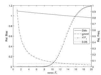
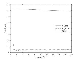
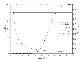
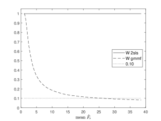
Figure 1: Top: Moderate Endogeneity. Bottom: High Endogeneity. Left: Bias of 2SLS and GMMf estimators relative to OLS bias, and $\widehat{F}_{r}$-based weak-instrument test rejection frequencies, $\alpha=0.05$, $\tau=0.10$, least-squares benchmark bias. The “0.05” line refers to the rej. freq. Right: Rejection frequencies of robust Wald tests, $\alpha=0.05$.

The left panels of Figure 1 displays the relative bias of the 2SLS and GMMf estimators, relative to that of the OLS estimator, as a function of the mean values of the robust F-statistic $\widehat{F}_{r}$, together with the rejection frequency of the $\widehat{F}_{r}$-based test for weak instruments, using the critical values from the least-squares benchmark bias. We present the relative bias here to be in line with the homoskedastic case as presented below. Different values of $\widehat{F}_{r}$ are obtained by different values of the scalar $e$ when setting the first-stage parameters $\pi=e\pi_{0}$. The relative bias of the GMMf estimator decreases quite rapidly with increasing values of $\widehat{F}_{r}$. For the moderate endogeneity case, the test has a rejection frequency of $5\%$ at a mean $\widehat{F}_{r}$ of $10.03$, with the relative bias of the GMMf estimator at that point equal to $0.092$. As shown in the top right-hand panel of Figure 1, the GMMf estimator based Wald test is well behaved in terms of size, with hardly any size distortion for mean values of $\widehat{F}_{r}$ larger than 5. The GMMf relative bias picture for the high-endogeneity case is very similar to that of the moderate-endogeneity case. Here the $\widehat{F}_{r}$ based test for weak instruments has a rejection frequency of $5\%$ at a mean $\widehat{F}_{r}$ of $8.98$, with the relative bias there being $0.091$. As for the homoskedastic case, where the Wald test size deviation from nominal size is larger for larger values of $\rho_{uv_{2}}^{2}$, the GMMf Wald test has a worse size performance in the high-endogeneity design, and has a $10\%$ rejection frequency at a mean $\widehat{F}_{r}$ of $26.64$. This would imply a critical value at the $5\%$ level of around $32$, which compares to the Stock and Yogo weak-instruments critical value of $38.54$ for a Wald test size of $10\%$ at the $5\%$ nominal level.

4.3.2 Homoskedastic Design

We next consider the homoskedastic design for the moderate endogeneity case with $\Sigma_{uv_{2}}=\frac{1}{G}\sum_{g=1}^{G}\Sigma_{uv_{2},g}$, resulting in

$$\Sigma_{uv_{2}}=\left[\begin{array}[]{cc}2.57&-1.50\\ -1.50&2.46\end{array}\right],$$

with $\rho_{uv_{2}}=-0.59$, as above. We consider smaller sample sizes of $n=250$ and $n=500$, or group sizes of $25$ or $50$ on average, to compare the weak-instrument finite sample behaviour of the GMMf estimator to that of the 2SLS estimator. In particular, the noise induced by estimation of $W_{2}^{-1}$ may adversely affect the GMMf estimator.

The results in Figure 2 shows that for this design and sample sizes the relative biases and Wald rejection frequencies are virtually identical for the two estimators, with the standard deviations of the GMMf estimates slightly larger than those of the 2SLS estimator, as expected. The rejection frequencies of the $\widehat{F}_{r}$-based test are here closer to those of the standard Stock and Yogo $\widehat{F}$-based test compared to the rejection frequencies of the $\widehat{F}_{\text{eff}}$-based test, with the latter test more conservative.

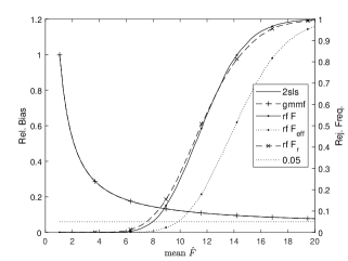
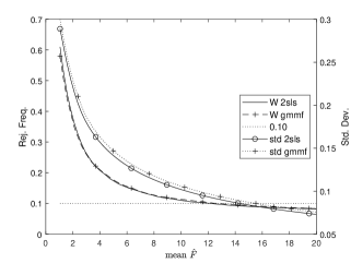
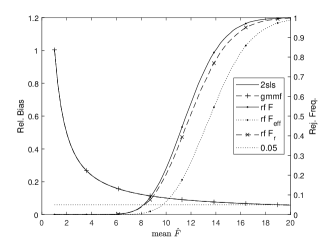
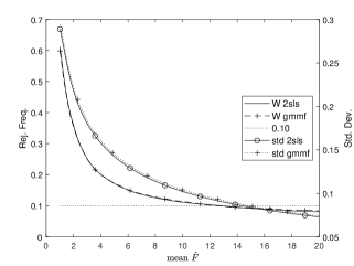
Figure 2: Homoskedastic design, moderate endogeneity. Top: $n=250$. Bottom: $n=500$. Left: Relative bias and weak-instrument tests rejection frequencies. Right: Wald test rejection frequencies and standard deviations of 2SLS and GMMf estimates.

5 Considerations for Practice and an Application

The grouped-data IV designs above are quite extreme in the variation of $\sigma_{v_{2},g}^{2}$, leading to the large differences between the values of $\widehat{F}_{\text{eff}}$ and $\widehat{F}_{r}$ and between the performances of the 2SLS and GMMf estimators. Note that these results carry over to a model with a constant and a full set of mutually exclusive binary indicators as instruments, when the variances $\sigma_{v_{2},g}^{2}$ for at least two groups are relatively small and their $\pi_{g}$ coefficients are different. This is the case if we for example change $\sigma_{v_{2},2}^{2}$ in the moderate endogeneity design above to be equal to the small $\sigma_{v_{2},1}^{2}$. An example where this could be relevant is from Stevenson (2018) who studies the effect of pretrial detention on conviction, using judge indicators as instruments, as cases are randomly assigned to judges. As the treatment is here binary, with variance $\pi\left(1-\pi\right)$, a very lenient (small $\pi$) and a very strict judge (large $\pi$) in terms of sending defendants to pretrial detention have small values of $\sigma_{v_{2}}^{2}$, but clearly different values of $\pi$. Unlike the 2SLS estimator, the GMMf estimator takes the differential strengths of the instruments due to the different values of $\sigma_{v_{2}}^{2}$ into account, giving more weight to very lenient and very strict judges. This could then lead to a better performance of the GMMf estimator in terms of bias, which would be indicated by the values of $\widehat{F}_{\text{eff}}$ and $\widehat{F}_{r}$.

For any application, one should therefore check whether there is a difference between the values of $\widehat{F}_{\text{eff}}$ and $\widehat{F}_{r}$. From the expressions of the 2SLS and GMMf estimators as given in (4) and (6) and the results for the grouped-data IV example, it is clear that the weights for the 2SLS estimator are determined only by the values of $\widehat{\pi}$ and the variance of the instruments $Z$, whereas the GMMf weights take into account first-stage nonhomoskedasticity through the robust estimator of the variance of $\widehat{\pi}$. If the nonhomoskedasticity is such that these weights are very different for the two estimators, and if the situation is as in the Andrews (2018) examples above that $cv_{r}<\widehat{F}_{r}>\widehat{F}_{\text{eff}}<cv_{\text{eff}}$, then the GMMf estimator is preferred from the weak-instruments test results in terms of Nagar bias. In Stata, StataCorp. (2023), the robust first-stage F-statistic is provided with the output of “ivregress” or “ivreg2”, Baum, Schaffer, and Stillman (2010), whereas “weakivtest”, Pflueger and Wang (2015), calculates $\widehat{F}_{\text{eff}}$ and critical values for the weak-instruments test. An extended version of the latter, called “gfweakivtest” also calculates the robust F-statistic and its weak-instruments critical values. It further includes the critical values based on the least-squares benchmark bias for both $\widehat{F}_{r}$ and $\widehat{F}_{\text{eff}}$, and presents the estimation results for the GMMf estimator.

A study with a set of mutually exclusive binary indicators as instruments, and one of the American Economic Review studies as considered in the review paper by Andrews et al. (2019), is Stephens and Yang (2014), who study the effect of schooling on wages, using data from the 1960-1980 US Censuses of Population. The endogenous variable is years of schooling for individual $i$, born in state $s$ in year $t$, and the instruments are three indicator variables $RS7$, $RS8$ and $RS9$, corresponding to being required to attend seven, eight or nine or more years of schooling, respectively. All specifications include state-of-birth and year-of-birth fixed effects, and the computed standard errors are robust to heteroskedasticity and clustering at the state-of-birth/year-of-birth cell. Stephens and Yang (2014) report the robust first-stage F-statistics $\widehat{F}_{r}$ in their Table 1, which presents estimates of the returns of schooling on log weekly wages for different samples, but do not present results for the effective F-statistic. As the estimator used is the 2SLS estimator, it is therefore important to consider whether the $\widehat{F}_{r}$ statistic misrepresents weak-instruments bias of the 2SLS estimator, in the sense that a large value of $\widehat{F}_{r}$ may not be an indicator of a good performance of the 2SLS estimator.

Table 3 replicates the estimation results of Table 1 in Stephens and Yang (2014, p 1784), and adds the values of $\widehat{F}$ and $\widehat{F}_{\text{eff}}$ together with the weak-instruments critical values for both $\widehat{F}_{r}$ and $\widehat{F}_{\text{eff}}$. It further reports the estimation results for the GMMf estimator. We present here the estimated standard errors of the 2SLS and GMMf estimators, Stephens and Yang (2014) instead presented weak-instruments robust confidence intervals based on the CLR test of Moreira (2003), robust to clustering using the methods of Finlay and Magnusson (2009). We further present the p-values of the test for overidentifying restrictions for the two-step Hansen $J$-statistic. The p-values of the robust Cragg-Donald rank statistics are identical and have been omitted from the table. The small p-values found for columns (5), (6) and (7) indicate significant heterogeneity of the effect estimates for the different instruments for these specifications. We will explore this further below for column (7).

The values of $\widehat{F}_{\text{eff}}$ and $\widehat{F}_{r}$ are quite similar across the specifications and both are smaller than the nonrobust $\widehat{F}$, for some specifications substantially smaller. The weak-instruments critical values for the $\widehat{F}_{r}$ statistic are smaller and vary less then those for $\widehat{F}_{\text{eff}}$. The choice of benchmark bias does not have a substantive effect on the critical values for both statistics. The null of weak instruments is rejected by the two statistics for the same specifications, with non-rejection in columns (2) and (8). The 2SLS and GMMf estimates and standard errors are very similar. It is clear that we do not have the situation here of a large value of $\widehat{F}_{r}$ accompanied by a small value of $\widehat{F}_{\text{eff}}$.

Table 3: The effect of schooling on log weekly wages, Stephens and Yang (2014, Table 1)

	White males		White males		All whites		Whites 25-54 born:
	ages 40-49		ages 25-54		ages 25-54		Non-south	South
	(1)	(2)	(3)	(4)	(5)	(6)	(7)	(8)
2SLS	0.096	-0.020	0.097	-0.014	0.105	-0.003	-0.009	0.019
	(0.016)	(0.041)	(0.010)	(0.021)	(0.011)	(0.016)	(0.012)	(0.043)
GMMf	0.095	-0.014	0.100	-0.012	0.111	0.004	0.015	0.022
	(0.016)	(0.040)	(0.010)	(0.021)	(0.011)	(0.016)	(0.011)	(0.044)
$\widehat{F}$	108.61	16.06	547.96	89.06	869.99	197.00	603.64	20.88
$\widehat{F}_{\text{eff}}$	42.85	8.11	64.17	24.38	62.98	42.40	34.40	6.13
$\widehat{F}_{r}$	42.76	8.22	81.37	23.63	91.73	40.57	67.25	6.34
$cv_{\text{eff}}$	9.21	10.31	13.50	10.36	14.65	11.10	16.30	9.49
$cv_{\text{eff}}^{LS}$	9.22	10.31	13.71	10.31	14.36	11.18	16.31	9.30
$cv_{r}$	8.64	8.73	8.74	8.74	9.62	8.65	8.96	8.82
$cv_{r}^{LS}$	8.63	8.69	8.86	8.69	9.03	8.70	8.85	8.96
$J$-test, p	0.81	0.27	0.12	0.22	0.00	0.00	0.00	0.07
Region$\times$yob	No	Yes	No	Yes	No	Yes	No	No
Controls	None	None	Age	Age	Age	Age	Age	Age
			quartic,	quartic,	quartic,	quartic,	quartic,	quartic,
			census yr	census yr	census yr,	census yr,	census yr,	census yr,
					gender	gender	gender	gender
$n$	609,852		2,166,387		3,680,223		2,566,127	1,114,096

Notes: All specifications include state-of-birth and year-of-birth fixed effects. Standard errors in brackets (), robust to heteroskedasticity and clustering at the state-of-birth/year-of-birth cell.

One interesting difference occurs in column (7). For the non-southern born the 2SLS estimate is negative. The CLR-based confidence interval as given in Table 1 of Stephens and Yang (2014) is $[-0.031,0.001]$ and Stephens and Yang (2014, p 1785) state “For the non-southern born shown in column (7), we continue to find a very strong first-stage relationship including a large $\widehat{F}_{r}$-statistic. However, we find a negative and nearly statistically significant estimate of the return to schooling.” Here the value of $\widehat{F}_{r}$ is equal to $67.25$, nearly double the value of $\widehat{F}_{\text{eff}}$, which is equal to $34.40$. Both $\widehat{F}_{\text{eff}}$ and $\widehat{F}_{r}$ do not indicate a weak-instruments problem in terms of Nagar bias for the 2SLS and GMMf estimators. The GMMf estimate here is positive and equal to $0.015$, (se $0.011$), moving away from a nearly statistically negative returns to schooling for this group as indicated by the CLR confidence interval. However, the robust Hansen two-step GMM J-statistic and robust Cragg-Donald rank statistic for overidentifying restrictions with two degrees of freedom have values of $22.05$ and $23.95$ respectively and p-values of $0.0000$, indicating significant heterogeneity in the estimated effect sizes for the different instruments.

To investigate this further, let $\widehat{\beta}_{ind}$ be the $k_{z}$-vector with $j$-th element $\widehat{\beta}_{ind,j}=\widehat{\pi}_{y,j}/\widehat{\pi}_{j}$. From (4) and (6) it follows that

$$\widehat{\beta}_{2sls} =\frac{\widehat{\pi}^{\prime}\left(V\widehat{a}r\left(\widehat{\pi}\right)\right)^{-1}\text{Diag}\left(\widehat{\pi}\right)\widehat{\beta}_{ind}}{k_{z}\widehat{F}}=\widehat{w}_{2sls}^{\prime}\widehat{\beta}_{ind};$$

$$\widehat{\beta}_{gmmf} =\frac{\widehat{\pi}^{\prime}\left(V\widehat{a}r_{r}\left(\widehat{\pi}\right)\right)^{-1}\text{Diag}\left(\widehat{\pi}\right)\widehat{\beta}_{ind}}{k_{z}\widehat{F}_{r}}=\widehat{w}_{gmmf}^{\prime}\widehat{\beta}_{ind}.$$

$\widehat{\beta}_{ind,j}$ is the just identified IV estimator with $Z_{j}$ as the excluded instrument, but with the other instruments $Z_{\left\{-j\right\}}$ included in the model as explanatory variables, see Windmeijer et al. (2021) and Masten and Poirier (2021). In order for a better comparison of the results for the individual instruments, we transform them linearly as $SRS7=RS7+RS8+RS9$, $SRS8=RS8+RS9$ and $SRS9=RS9$, corresponding to being required to attend seven or more, eight or more, or nine or more years of schooling, respectively. Clearly, this does not change the estimation results for the 2SLS and GMMf estimators, but using each of these transformed instruments as the excluded instrument in turn has a clear group comparison and the transformation does affect the values of $\widehat{\beta}_{ind}$ and the 2SLS and GMMf weights. From the reduced-form and first-stage specifications (3) and (2), it follows that $\beta_{ind,j}\coloneqq\pi_{y,j}/\pi_{j}=\beta$, for $j=1,\ldots,k_{z}$, and the overidentification test can be formulated as a test for $H_{0}:\beta_{ind,1}=\beta_{ind,2}=\ldots=\beta_{ind,k_{z}}$, see Windmeijer (2019).

Table 4 presents the results for $\widehat{\pi}$, $\widehat{\beta}_{ind}$ and the 2SLS and GMMf weights for the specifications of columns (1) and (7) in Table 3. For column (1), the p-value of the overidentification test statistic is large, and the values of $\widehat{\beta}_{ind,j}$ are all positive, with ordered values of $0.07$, $0.10$ and $0.14$. The 2SLS and GMMf weights are very similar, resulting in the virtually identical estimates of $0.0955$ and $0.0953$. For column (7), we find very different values of $\widehat{\beta}_{ind,j}$. These are given by $-0.14$, $0.03$ and $0.18$, with the estimated variance of $\widehat{\beta}_{ind}$ such that the null of equal $\beta_{ind,j}$ is rejected by the overidentification test statistic. The large negative value is associated with the $SRS8$ instrument, the one indicating that an individual is required to attend eight or more years of schooling. The 2SLS and GMMf weights are now different, with the GMMf estimator giving less weight to the negative value, resulting in a small positive estimate $\widehat{\beta}_{gmmf}$, whereas $\widehat{\beta}_{2sls}$ is negative. But the large heterogeneity in estimated effect sizes, by essentially the same type of instruments, needs to be investigated and makes it difficult to interpret any linear combination of these estimates.

Table 4: Some Further Estimation Results

Column	Inst	$\widehat{\pi}$	$se_{\widehat{\pi}}$	$se_{\widehat{\pi},r}$	$\widehat{\beta}_{ind}$	$se_{\widehat{\beta}_{ind},r}$	$\widehat{w}_{2sls}$	$\widehat{w}_{gmmf}$
(1)	$SRS7$	0.095	0.023	0.036	0.137	0.089	0.126	0.128
	$SRS8$	0.129	0.018	0.028	0.071	0.041	0.348	0.356
	$SRS9$	0.180	0.015	0.024	0.102	0.024	0.526	0.517
(7)	$SRS7$	0.212	0.014	0.056	0.177	0.045	0.257	0.290
	$SRS8$	0.206	0.010	0.057	-0.140	0.057	0.454	0.347
	$SRS9$	0.156	0.006	0.020	0.033	0.018	0.289	0.362

Notes: Column numbers refer to those in Table 3. Instrument $SRSj$ indicates being required to attend $j$ or more years of schooling.

6 Concluding Remarks

For models with a single endogenous explanatory variable, we have introduced a class of generalized effective F-statistics as defined in (8) in relation to a class of linear GMM estimators given in (7) and have shown that the Montiel Olea and Pflueger (2013) weak-instruments testing procedure that they established for the effective F-statistic in relation to the Nagar bias of the 2SLS estimator applies to this extended class. In particular, the standard nonhomoskedasticity robust F-statistic is a member of this class and is associated with the behaviour in terms of Nagar bias of the novel GMMf estimator, which has its weight matrix based on the first-stage residuals. We then focused on a comparison of the effective F-statistic and the robust F-statistic and the associated weak-instrument behaviours of the 2SLS and GMMf estimators. In particular, we have shown that and explained why the GMMf estimator’s performance is much better in terms of bias than that of the 2SLS estimator in the grouped-data designs of Andrews (2018), where the robust F-statistic can take very large values, but the effective F-statistic is very small. One should therefore in general not use the robust F-statistic to gauge instrument strength in relation to the performance of the 2SLS estimator, Andrews et al. (2019, pp 738-739), but as shown here, it can be used as a weak-instrument test in relation to the Nagar bias of the GMMf estimator. In practice, therefore, both the effective F-statistic and robust F-statistic should be reported, together with their critical values, and the GMMf estimator considered in cases where there is a clear discrepancy with a large value for the robust F-statistic. We found no such discrepancy in the applied analysis of Stephens and Yang (2014).

We have not focused here on the wider applicability of the class of generalized effective F-statistics and their associated GMM estimators, but an example is the one-step Arellano and Bond (1991) GMM estimator for panel data models with a single endogenous variable. Two-step estimators do not fall in the class because of the presence of estimated structural parameters in the weight matrix, but one could test for weak instruments in this setting, fixing the parameter of the endogenous variable in the weight matrix, for example under a specific null value of interest.

A topic for future research for the general nonhomoskedastic setting is an extension to the linear model with more than one endogenous variable. Lewis and Mertens (2022) is an extension of the Montiel Olea and Pflueger (2013) method to the multiple endogenous variable case for the 2SLS estimator, but they do not consider such an extension for the wider class of GMM estimators. Future research should also address the weak-instruments Wald size properties for both the single and multiple endogenous variables settings.

References

• Andrews (2018) Andrews, I. (2018): “Valid Two-Step Identification-Robust Confidence Sets for GMM,” The Review of Economics and Statistics, 100, 337–348.
• Andrews et al. (2019) Andrews, I., J. H. Stock, and L. Sun (2019): “Weak Instruments in Instrumental Variables Regression: Theory and Practice,” Annual Review of Economics, 11, 727–753.
• Angrist (1991) Angrist, J. D. (1991): “Grouped-Data Estimation and Testing in Simple Labor-Supply Models,” Journal of Econometrics, 47, 243–266.
• Angrist and Pischke (2009) Angrist, J. D. and J.-S. Pischke (2009): Mostly Harmless Econometrics. An Empiricist’s Companion, Princeton University Press.
• Arellano and Bond (1991) Arellano, M. and S. Bond (1991): “Some Tests of Specification for Panel Data: Monte Carlo Evidence and an Application to Employment Equations,” The Review of Economic Studies, 58, 277.
• Baum et al. (2010) Baum, C. F., M. E. Schaffer, and S. Stillman (2010): “ivreg2: Stata Module for Extended Instrumental Variables/2SLS, GMM and AC/HAC, LIML and k-Class Regression,” http://ideas.repec.org/c/boc/bocode/s425401.html.
• Bekker and Ploeg (2005) Bekker, P. A. and J. Ploeg (2005): “Instrumental Variable Estimation Based on Grouped Data,” Statistica Neerlandica, 59, 239–267.
• Bun and de Haan (2010) Bun, M. and M. de Haan (2010): “Weak Instruments and the First-Stage F-Statistic in IV Models with a Nonscalar Error Covariance Structure,” Tech. Rep. Discussion Paper: 2010/02, University of Amsterdam.
• Finlay and Magnusson (2009) Finlay, K. and L. M. Magnusson (2009): “Implementing Weak-Instrument Robust Tests for a General Class of Instrumental-Variables Models,” The Stata Journal, 9, 398–421.
• Lewis and Mertens (2022) Lewis, D. J. and K. Mertens (2022): “A Robust Test for Weak Instruments with Multiple Endogenous Regressors,” Working Papers 2208, Federal Reserve Bank of Dallas.
• Masten and Poirier (2021) Masten, M. A. and A. Poirier (2021): “Salvaging Falsified Instrumental Variable Models,” Econometrica, 89, 1449–1469.