drnxxx
S. Mahajan, A. Khan, M.T. Mohan
Finite element approximation for a delayed generalized Burgers-Huxley equation with weakly singular kernels: Part I Well-posedness, Regularity and Conforming approximation
Abstract
The analysis of a delayed generalized Burgers-Huxley equation (a non-linear advection-diffusion-reaction problem) with weakly singular kernels is carried out in this work. Moreover, numerical approximations are performed using the conforming finite element method (CFEM). The existence, uniqueness and regularity results for the continuous problem have been discussed in detail using the Faedo-Galerkin approximation technique. For the numerical studies, we first propose a semi-discrete conforming finite element scheme for space discretization and discuss its error estimates under minimal regularity assumptions. We then employ a backward Euler discretization in time and CFEM in space to obtain a fully-discrete approximation. Additionally, we derive a prior error estimates for the fully-discrete approximated solution. Finally, we present computational results that support the derived theoretical results. Burgers-Huxley equation, Galerkin approximation, weak solution, A priori error analysis, Conforming finite element method.
1 Introduction
The generalized Burgers-Huxley equation (GBHE) with weakly singular kernels describes a prototype model for describing the interaction between reaction mechanisms, convection effects and diffusion transports with delays. The GBHE has various applications in different fields such as traffic flows, nuclear waste disposal, the mobility of fish populations, motion of the domain wall of a ferroelectric material in an electric field, etc. In this work, we consider a delayed generalized Burgers-Huxley equation with weakly singular kernels defined on , where be an open bounded and simply connected convex domain with Lipschitz boundary . The delayed GBHE under our consideration is given by
| (1) |
where is a weakly singular kernel, is an external forcing, are parameters such that is the advection coefficient, , is the retardation time, is the relaxation time, and . The integration term is used to study the delayed effect.
For , the equation (1) becomes
which is the generalized Burgers-Huxley equation (GBHE). A wide literature is available on the GBHE and related models. Solitary and travelling wave solutions of the generalized Burgers-Huxley equation using a relevant non-linear transformation is obtained (Wang et al. (see 1990); Ablowitz et al. (see 1987); El-Danaf (see 2007); Wazwaz (see 2005), etc). The global solvability results for the stochastic generalized Burgers-Huxley (SGBH) equation have also been proved in Kumar & Mohan (2022). Many researchers have established numerical solutions of the GBHE by using various numerical techniques such as Hashim et al. (2006) used an Adomian decomposition method, Khattak (2009) provided a numerical solution of GBHE based on the collocation method using mesh-less radial basis functions, Sari et al. (2011) performed numerical studies using a fourth-order Runge-Kutta (RK4) scheme in time combined with up to tenth-order finite difference scheme in space, Kumar et al. (2011) used a three-step Taylor–Galerkin finite element scheme to approximate the solution of the singularly perturbed GBHE.
For , , and , the equation (1) is known as the Burgers-Huxley equation (see Wang et al. (1990); Wazwaz (2009), etc.). For , and , the equation (1) takes the form which is known as the Huxley equation which describes the nerve pulse propagation in nerve fibres and wall motion in liquid crystals (see Wang, 1985). For , , and , the equation (1) reduces to the well-known viscous Burgers’ equation which represents the mathematical modelling of the turbulence phenomena (see Burgers, 1948), far field of wave propagation in non-linear dissipative systems, shock wave theory, vorticity transportation, heat conduction, wave processes in thermoelastic medium, dispersion in porous media, hydrodynamic turbulence, elasticity, gas dynamics, etc.
The kernel function is weakly singular such that . Moreover, we assume that the function is a positive kernel, that is, if for any , we have
| (2) |
One primary example of the weakly singular kernel is given by
where is the Euler Gamma function. The convolution integral can be interpreted as a fractional integral of order (see, e.g., Adolfsson et al., 2003; Oldham & Spanier, 1974). By varying the fractional integral exponent, we obtain a link between parabolic behavior (in the limit the kernel approaches to the delta distribution) and hyperbolic behavior (specializing ). The global solvability and numerical studies, for the one dimensional GBHE and the two-dimensional stationary generalized Burgers- Huxley equation, have been recently established in Mohan & Khan (2021) and Khan et al. (2021), respectively. The literature relevant to the finite element analysis of integro-differential equations of parabolic type is vast. The time discretization for integro-differential equations with a smooth kernel was introduced in Sloan & Thomée (1986). A prior error estimates for linear parabolic equations can be found in Cannon & Lin (1987) and Pani & Peterson (1996), and for both parabolic and hyperbolic equations in Yanik & Fairweather (1988). Error estimates for the semi-discrete finite element method (FEM) have been discussed in Thomée & Zhang (1989). Time discretization and error estimation using the Crank-Nicolson scheme and Padé-type scheme are discussed in Cannon & Lin (1988) and Zhang (1993), respectively.
Fully-discrete FEM for parabolic integro-differential equations with a weakly singular kernel using positive quadrature rule has been discussed in Chen et al. (1992) and McLean & Thomée (1993) . A second-order accurate numerical method for a semi-linear integro-differential equation using the Crank-Nicolson scheme with a weakly singular kernel is discussed in Mustapha & Mustapha (2010). Recently, Zhou et al. (2019) used the weak Galerkin finite element scheme for the parabolic integro-differential equation with a weakly singular kernel to obtain the optimal convergence order in .
To the best of the authors’ knowledge, this work appears to be the first in the field of theoretical and numerical partial differential equations to investigate the solvability of the model generalized Burgers-Huxley equation with memory (1). This research article makes significant contributions from both theoretical and numerical perspectives:
-
•
Well-posedness results: From theoretical point of view, the well-posedness of the generalized Burgers-Huxley equation with memory (Kernel) is proven for the first time in the literature (Section 2.3). The analysis is carried out in an open bounded and simply connected convex domain, , with a Lipschitz boundary .
- •
-
•
Semi-discrete error estimates: This work provides, for the first time, semi-discrete error estimates for non-linear integro-differential equations with weakly singular kernels under minimal regularity assumptions.
-
•
Fully-discrete FEM error estimates: The major contribution in the numerical aspect lies in the error estimates for the fully-discrete finite element method (FEM). Unlike the previous literature that necessitates (Thomée (2007)) to handle the time derivative term, which requires the boundary to be at least , our results do not impose such higher regularity requirements. Notably, the minimum regularity result has been established for the linear parabolic equation Hou & Zhu (2006), but our work is the first to extend it for a non-linear equation with weakly singular kernels.
We show the existence and uniqueness of a global weak solution to the system (1), using a Faedo-Galerkin method. Regularity results of the weak solution are obtained under smoothness assumptions on the initial data and external forcing. Here, we propose the conforming finite elements (CFEM) scheme to obtain the numerical approximation of the exact solution under minimal regularity and the required regularity is also proved for GBHE with weakly singular kernels. We rigorously derive a priori error estimates indicating first-order convergence in both space and time of the CFEM. We also include a set of computational tests that confirm the theoretical error bounds and show some model equation properties. The finite element approximation using non-conforming and discontinuous Galerkin (DG) finite element method has been discussed in Mahajan & Khan (Prep).
The paper is organized as follows: In section 2, we will discuss the notational conventions and provide the abstract formulation of our problem with the necessary functional spaces. The global solvability results for the system (1) are established in Theorem 2.5; that is, the existence and uniqueness of a global weak solution is proved by taking the initial data and external forcing . The uniqueness result of weak solutions under different choices on the initial data is discussed in Theorem 2.8. The regularity results are obtained in Theorem 2.12 and Theorem 2.14 under smoothness assumptions on the initial data and the external forcing. In the subsequent section, the semi-discrete and the fully-discrete scheme are introduced, and a priori error estimates are derived for the CFEM in section 3. Finally, numerical results are presented in section 4 for 2D and 3D to support our theoretical results.
2 Mathematical Setting and Solvability
This section lists necessary function spaces and notations used throughout the paper. Also, we define the operators used to obtain the global solvability results of the system (1), discuss its properties and establish the existence of a unique weak solution for our system and its regularity.
2.1 Functional setting
We use the standard notation for function spaces. In particular, the Lebesgue spaces are denoted by for and the corresponding norm is denoted by (omitting the domain specification whenever clear from the context). For , is a Hilbert space with the inner product denoted by . The Hilbertian Sobolev spaces are denoted by . Let denote the space of all infinitely differentiable functions with compact support in and be the closure of in -norm. As is a bounded domain, defines an equivalent norm on by using the Poincaré inequality. Moreover, we have the Gelfand triplet , where is the dual of , and the embedding is compact. The duality paring between and as well as and its dual , where is denoted by . The sum space is well defined and
where which is equivalent to the norms and , and
Note that and are Banach spaces. Moreover, we have the continuous embedding . The following operators will be used in further analysis:
2.1.1 Linear operator
Let be the unbounded and self-adjoint linear operator on defined by:
whenever is convex, bounded open subset of with a boundary (Theorem 3.1.2.1, Grisvard (1985)). Note that , for and , using the Sobolev Embedding Theorem (see Mitrovic & Zubrinic, 1997). As the embedding is compact, exists and is a symmetric compact operator on . Then, by using spectral theorem (see Dautray & Lions, 1990), there exists a sequence of eigenvalues of , and an orthonormal basis of consisting of eigenfunctions of (see Dautray & Lions, 1990, p. 504).
An integration by parts yields
so that .
2.1.2 Non-linear operators
Let us define the non-linear operator by
The map is well-defined since so that we can define a mapping by . For simplicity, we use the notation .
For all and , using an integration by parts and boundary conditions, we have
The above expression implies
| (3) |
Let us now show that the operator is locally Lipschitz. For and , using integration by parts and Taylor’s formula for , we have
so that
| (4) |
for all . Therefore, the operator is locally Lipschitz.
Let us now consider the non-linear operator . It should be noted that
| (5) |
for all . Using Taylor’s formula and Hölder’s inequality, for with , and , we get
| (6) | ||||
for , where is the Lebesgue measure of . Thus, the operator is locally Lipschitz.
The following lemmas are useful for the further analysis:
Lemma 2.1.
(Mohan, 2020) Let and for some . Then
Lemma 2.2 (Remark A.2, Mohan & Sritharan (2019)).
If the kernel satisfies the conditions
then for any right continuous function with left limits and for such that is well defined, we have
| (7) |
2.2 Abstract formulation
By using the above functional setting, the abstract formulation of the system (1) is given by
| (8) |
for a.e. , where
Let us now provide the definition of weak solution of the system (8).
Definition 2.4 (Weak solution).
For the initial data and external forcing , we say that a function
with
is called a weak solution to the system (8), if, for a.e. , satisfies:
for any .
2.3 Existence and uniqueness of weak solution
Let us now discuss the existence and uniqueness of the weak solution for the system (1).
Theorem 2.5 (Existence of a weak solution).
Proof 2.6.
We establish the existence of a weak solution to the system (1) in the following steps: Step 1: Faedo-Galerkin approximatiiron. Let the set be an orthogonal basis of and orthonormal basis of (page 504, Dautray & Lions (1990)). We look for a function of the form , where is a fixed positive integer and the coefficients , for and are selected so that , for and
| (9) |
for a.e. and . As the non-linear operators are locally Lipschitz (see (2.1.2) and (6)) using Carathéodory’s existence theorem, the finite dimensional problem (2.6) has a local solution , where . Step 2: -energy estimate. Multiplying (2.6) by , and then summing for , we have
for a.e. . Using the property of the non-linear operator (3) and the estimate (2.1.2) , we get
Integrating the above inequality from to , we have
| (10) |
for all , where we have used the fact that . Using (2) and an application of Gronwall’s inequality in (2.6) yields
for all . Taking supremum over time , we have
| (11) |
and the right hand side of the inequality (2.6) is independent of . Step 3: Estimate for the time derivative. For any , with , we have
An application of the Cauchy-Schwarz inequality and Hölder’s inequality yield
Taking supremum over all , we have
Integrating from 0 to T and using Young’s inequality, we arrive at
| (12) |
where is bounded since (cf. Lemma 2.1)
and
Step 4: Passing to limit. As the energy estimates (2.6) and (2.6) are uniformly bounded and independent of , using the Banach-Alaoglu theorem, we can extract a subsequence of such that
| (13) |
as , for all . Since we have compact embedding of (page 284, Evans (2010)), an application of the Aubin-Lions compactness lemma yields the following strong convergence:
| (14) |
as . The above strong convergence also implies , for a.e. as (that is, along a subsequence). Let us now take limit in (2.6) along the subsequence . Choose a function having the form where are given smooth functions and is a fixed integer. Let us choose , multiply (2.6) by , sum from to and then integrate it from to to find
| (15) |
Setting (more specifically ) and using the convergences given in (13) and (14), we can take weak limit in (2.6) to obtain
| (16) |
provided if we show that
Using density argument is dense in , we will show that for all to obtain that , as . By an application of Taylor’s formula, integration by parts, Hölder’s inequality, and convergence, we obtain
Again using Taylor’s formula, interpolation and Hölder’s inequalities, , we find
which completes the convergence proof. Step 5: Initial data. Let us now show that . From (2.6), we note that
| (17) |
for each with . In a similar fashion, we deduce from (2.6) that
Taking in the above expression, using the above convergences ((13) and (14)) and passing then to limit, we find
| (18) |
since as in . As is arbitrary, comparing (2.6) and (2.6), one can easily conclude that in . Step 6: Energy equality. As with using an argument similar to Theorem 7.2 (Robinson & Pierre (2003) (Exercise 8.2)) we have and the following energy equality holds
for all This proves the existence of weak solution.
Remark 2.7.
If we take the initial data , and the external forcing, , then we can obtain the -energy estimate as follows:
Multiplying (2.6) by , and then summing for , we obtain for a.e.
Now, using (3), the Cauchy-Schwarz, Hölder’s and Young’s inequalities, we arrive at
for a.e. . Integrating the above inequality from to and using Lemma 2.2 and Remark 2.3, we have
for all . Applying Gronwall’s inequality, we get
for all . Thus, it is immediate that
| (19) |
and the right hand side of the above inequality is independent of . Since the right hand side of (2.7) is independent of , an application of the Banach-Alaoglu theorem yields .
We will now discuss a result on the uniqueness of the weak solution that we have obtained in Theorem 2.5.
Theorem 2.8 (Uniqueness of weak solution).
Proof 2.9.
Let and be two weak solutions of the system (1) with the same external forcing and initial data with the regularity given in the statement. Then, satisfies:
for in the weak sense. One can write the above system in the weak sense as
| (20) |
for all and a.e. . Using in (20), we find
| (21) |
It can be easily seen that
| (22) |
Estimating the term from (2.9) as
| (23) |
We estimate the term from (2.9), using Taylor’s formula, Hölder’s and Young’s inequalities as
| (24) |
Combining (2.9)-(2.9) and substituting it in (2.9), we obtain
| (25) |
On the other hand, we derive a bound for , using Taylor’s formula, Hölder’s, Ladyzhenskaya’s and Young’s inequalities as
| (29) | ||||
| (33) | ||||
| (34) |
where . Combining (2.9) and (29), we have
| (35) |
for a.e. . An application of Gronwall’s inequality in (2.9) gives for all
| (36) |
For and , from Remark 2.7, it is clear that , and hence the uniqueness follows. For , the integral appearing in the exponential is finite by using interpolation inequality as
Hence, the uniqueness follows if we take the initial data .
Remark 2.10.
For , using Gagliardo-Nirenberg’s inequality in (29), one can find a sufficient criterion for the uniqueness of weak solution for as
Remark 2.11.
If we consider our initial data and then there exists a unique weak solution to the system (1). One can estimate in (29) using integrating by parts, Taylor’s formula, Hölder’s and Young’s inequalities as:
| (40) | ||||
| (44) | ||||
| (45) |
Combining (2.9) and (40) in (21), we find
From the above expression, it is immediate that
For , integrating the above inequality from to , (2) and then applying of Gronwall’s inequality results to
for all . Since and and are weak solutions of the system (1), uniqueness follows easily.
2.4 Regularity results
If we take our initial data , and the external forcing, , where is either convex, or a domain with -boundary, then we can obtain the -energy estimate. Under smoothness assumptions on the domain, initial data and external forcing, let us now establish the regularity of the weak solution obtained in Theorem 2.5.
Theorem 2.12 (Regularity).
Let be a weak solution to the system (1). If is either convex, or a domain with -boundary and let and be given. Then, is a strong solution with
and and the following system is satisfied:
for a.e. .
Proof 2.13.
Step 1: -energy estimate. Let denote the eigenvalue of in . Multiplying the identity (2.6) by and summing it from , we have
| (46) |
Now, using integrating by parts and applying Hölder’s and Young’s inequalities, we find
Estimating using Hölder’s and Young’s inequalities as follows:
Combining the above estimates and substituting in (46), we get
Integrating from to and using (2), we find
| (47) |
since satisfies the energy estimates (2.6) and (2.7). Whenever and , from (2.13), we have
by using the elliptic regularity (Theorem 3.1.2.1, Grisvard (1985)). Using Sobolev’s inequality, , we have so that
Thus, we infer
Step 2: Estimate for time derivative. For , multiplying (2.6) by and sum it over we have
| (48) |
Using Hölder’s and Young’s inequalities, we estimate the first term from the right hand side of the equality (2.13) as
| (49) |
Similarly, we estimate and as
| (50) |
The final term from the right hand side of the equality (2.13) can be estimated as
| (51) |
Combining (49)-(51), substituting it in (2.13) and then integrating from to , we get
Applying Gronwall’s inequality, we arrive at
| (52) |
for all . Using the estimate given in (2.13), we obtain that the right hand side of (2.13) is independent of . Thus, it is immediate that . Using arguments similar to Steps 4 and 5 in Theorem 2.5, we obtain the existence of a such that
so that we get and is a strong solution to the system (1). The uniqueness follows from the estimate (36) and we have .
Theorem 2.14.
Let for and, for and assume that
-
(i)
If , then, we have
-
(ii)
If then .
Proof 2.15.
We divide the proof into the following steps: Step 1. , and .
Let for and, for . Differentiating (2.6) with respect to , we find
| (53) |
Multiplying (2.15) with and summing it over , we obtain
| (54) |
We estimate the term using integration by parts, Hölder’s, Ladyzhenskaya’s inequality and Young’s inequalities as
| (55) |
We estimate as
Similarly, we estimate the terms and as
| (56) |
Substituting the estimates (2.15)-(2.15) in (2.15), we have
where and .
As and note that (see page 385, Evans (2010)) and an application of Gronwall’s inequality yields
| (57) |
for all , where the first term in exponential is bounded , provided , for and, for . Taking supremum over time , we have
Step 2. .
In (2.6), if we take , then we have for a.e.
| (58) |
Using integration by parts, one can estimate the time derivative term as
Using the above estimate, (2.15) can be rewritten as
| (59) |
for a.e. . For the term , using integration by parts and Young’s inequality, we get
An application of Cauchy-Schwarz and Young’s inequalities yields
Combining the above estimates and integrating from to , and using Lemma 2.2 and Remark 2.3, we have
| (60) |
As , we have and , which implies , so we have
Using the last estimate and an application of Gronwall’s inequality in (2.15) yield
For the right hand side to be bounded, we need to show that . As , using Agmon’s inequality we have for
for . For the , for , using Agmon’s inequality , so
provided . Since is arbitrary, the above estimate is finite for . Hence . Step 3. .
Let denote the eigenvalue of in . Multiplying the identity (2.6) by and summing it from , we have
| (61) |
An application of integration by parts yields
| (62) |
Note that Since , using integration by parts, Cauchy-Schwarz and Young’s inequalities, we have
Now we estimate using Sobolev embedding (for , and for , ), Hölder’s and Young’s inequalities as
Combining, we have
Again using Cauchy-Schwarz and Young’s inequalities, we get
Finally, for the forcing term using Cauchy-Schwarz and Young’s inequalities, we obtain
Combing the above estimates we have
Integrating from to , using positivity of the kernel and Gronwall’s inequality, and taking supremum over time, we have
Using the estimate (2.13) and (2.15) the right hand side is bounded. Hence we have , . Passing limit along a subsequence , we obtain the required bound for .
Remark 2.16.
In Theorem 2.14 , we need for the memory term. However, if we take , that is, GBHE without memory using elliptic regularity we can prove that for and , we have .
3 Finite Element Method
3.1 Semidiscrete Galerkin approximation and error estimates
This section is devoted to the error estimates for the semidiscrete Galerkin approximation. We partition the domain into shape-regular meshes (triangular or rectangles) denoted by and consider a finite dimensional space , defined as
| (1) |
where is the space of polynomials which have degree at most . Note that, is a finite dimensional subspace of and is the associated small mesh parameter. The aim is to prove the estimate of the type (see Thomée, 2007)
for all . The continuous time Galerkin approximation of the problem (8) is defined in the following way: Find such that for ,
| (2) |
where approximates in . Central to the analysis of finite element methods, we define an elliptic projection associated to our model onto , the Ritz projection (Thomée (2007)) of defined by
By setting in the above equality, we obtain that the Ritz projection is stable, that is, , for all . If we take , then, we have the following estimate for (Thomée (2007)),
| (3) |
Theorem 3.1 (Existence of a discrete solution).
The discrete equation (3.1) admits at least one solution .
Proof 3.2.
It follows as a direct consequence of Theorem 2.5.
For all , the error estimates in this semi-discretization are given in the following theorem,
Theorem 3.3.
Note: If and , then using Theorem 2.12 we have .
Proof 3.4.
Using (2.4) and (3.1), we know that satisfies
| (5) |
for all and a.e. . Let us choose in (3.4) to obtain for a.e.
| (6) |
Next, we write as in (3.4) to find
| (7) |
for a.e. . Using calculations similar to (2.9) yields
| (8) |
where the positive constants and . We estimate and using the Cauchy-Schwarz and Young’s inequalities as
| (9) | ||||
| (10) |
Using an integration by parts, Taylor’s formula, Hölder’s and Young’s inequalities, we rewrite as
| (11) |
Let us rewrite as
| (12) |
We estimate using Taylor’s formula, Hölder’s and Young’s inequalities as
| (13) |
Using the Cauchy-Schwarz and Young’s inequalities, we estimate as
| (14) |
Making use of Taylor’s formula, Hölder’s, Young’s and Gagliardo-Nirenberg inequalities, we estimate as
| (15) |
where we used the fact that . Note also that
| (16) |
Combining (9)-(3.4) and then substituting it in (3.4), we deduce
Integrating the above inequality from to and using positivity of kernel , we have
| (17) |
for all , where we estimate the memory term using Lemma 2.1 as
for the constant . Using the Cauchy-Schwarz inequality and Young’s inequality, we estimate and as
Using the above estimates in (3.4) and then applying Gronwall’s inequality, we get
| (18) |
The term appearing in the exponential is uniformly bounded and is independent of for (see 36). Using (3), we get
Thus, (3.4) implies that
and hence the estimate (3.3) follows.
Remark 3.5.
1. For with and with , we infer from Theorem 2.14 . For large values of (cf. Remark 2.11), one can get the same regularity for the case with .
2. In the above Theorem we need . However, if we assume and denotes the projection from onto as in Hou & Zhu (2006) and Chrysafinos & Hou (2002), namely, for each
| (19) |
Also, there exists a constant independent of and such that
We can estimate the first term on the right hand side of (3.4) using the projection (19) repeatedly as
for a.e. , which upon integration can be estimated as
So, we need only our initial data and
3.2 Fully-discrete Galerkin approximation and error estimates
In this section, we introduce a fully-discrete conforming finite element scheme. We partition the time interval into with uniform time stepping , that is, . We replace the time derivative with a backward Euler discretization and approximating the memory term in the following way: We shall approximate in by the piecewise constant function taking value in and the quadrature rule as
where , for We denote as a generic constant which is independent of and . We then define a generic finite element approximate solution by
| (20) |
Note here that . The continuous time Galerkin approximation of the problem (8) is defined in the following way: Find for such that for :
| (21) |
for , approximates in and represent the nodes of the triangulation of .
The existence of the discrete solution can be proved using an application of Brouwer’s fixed point theorem [Lemma 1.4, Temam (2001)] as done in Theorem 3.1 Khan et al. (2021). To show the error estimates, we need a stability result. It is natural to see that for the quadratic form analogous to the double integral in (2), we have
| (22) |
as discussed in Mustapha & McLean (2009) and Lemma 4.7 McLean & Thomée (1993). The following lemma is useful for the analysis:
Lemma 3.6.
Assume Then the set defined by satisfies
and
If for some , then
Proof 3.7.
For a proof, we refer to Lemma 3.2, Hou & Zhu (2006).
Let us now discuss the stability of the fully-discrete approximation (21).
Lemma 3.8 (Stability).
Assume and . Let be defined by (21). Then
| (23) |
Proof 3.9.
Suppose , taking in (21), we obtain
Using (3), (2.1.2), Cauchy-Schwarz and Young’s inequalities, we have
This may be simplified as
Summing over for and using positivity of the Kernel (22) and Lemma 3.6, we have
Finally, an application of the discrete Gronwall inequality (Lemma 9 Pani & Peterson (1996)) yields the required bound (23).
Lemma 3.10.
Proof 3.11.
We divide our proof into two steps: In Step 1, we prove the error estimates on the nodal values and in Step 2, we prove the final estimate. Step 1: Estimates at Integrating the semi-discrete scheme (3.1) from to , we obtain
| (24) |
The fully-discrete scheme (21) is given as
| (25) |
Subtracting (3.11) from (3.11), we have
Rewriting the above equation and taking , we deduce
Using Cauchy-Schwarz and Young’s inequalities, we can estimate the first term on right hand side as
| (26) |
Again an application of the Cauchy-Schwarz and Young’s inequalities yield
where the first term on the right hand side can be estimated as
| (27) |
The memory term can be estimated as
where the term can be estimated using (3.11) as
where . An application of integration by parts and Cauchy-Schwarz inequality gives
| (28) |
Now, we estimate similar to (3.11) as
Finally the reaction term can be simplified as
Firstly, we estimate the term with coefficient , using Cauchy-Schwarz inequality and the estimate similar to (3.11) as
Using an estimate similar to (3.11), we have
Also for the final term, we obtain
for () and (). For, , we derive a bound for , using Taylor’s formula, Hölder’s, Gagliardo-Nirenberg interpolation and Young’s inequalities as
where . Combining the above estimates and using the calculations similar to (2.9), we deduce
Summing over all , and using the positivity of the kernel (cf. (22)), we attain
| (29) |
For the memory term, we get
Using the above estimate and an application of Gronwall inequality in (29) yields
| (30) |
One can prove the estimates obtained in (2.15) for the semi-discrete solution also, so that the right hand side of (3.11) is bounded (see Remark 3.14 below). Step 2: Estimate for any . Let us now introduce a linear interpolation for the semi-discrete solution [Yi & Guo (2015) (Section 3.1)] by:
Let us write , where is the linear interpolation as defined above. Using the triangle inequality, we have
The first term can be estimated using (Lemma 3.2 [Yi & Guo (2015)]) and the final term using (3.11) as
| (31) |
Again using triangle inequality, we have
Similarly as in (3.11), by using (Corollary 3.1 [Yi & Guo (2015)]) and the estimate (3.11), we deduce
and the required result follows.
The main result of this section is
Theorem 3.12.
Assume that and such that be the solution of (2.4) on the interval . Then, the finite element approximation converges to as . In addition, there exists a constant such that the approximation satisfies the following error estimate:
Remark 3.14.
-
1.
In the literature most of the estimates needs higher regularity but we have proved estimates under the minimal regularity assumptions.
-
2.
For the generalised Burgers- Huxley equation without memory (that is, ), we have obtained the optimal rate of convergence. Also, if we assume that then , so that we obtain the optimal convergence again.
- 3.
-
4.
If we assume , then we have , where . Therefore, the error estimates are of order For , that is, then we have the error estimates are of order .
- 5.
4 Numerical studies
In this section, we perform numerical computations to verify the theoretical results obtained in Theorem 3.12. The results are obtained in the open-source finite element library FEniCS (Alnæs et al., 2015; Langtangen & Logg, 2016).
The error tables shown below present the error estimates and order of convergence for the generalized Burgers-Huxley equation (GBHE) with kernel and without Kernel for the equation
| (32) |
under the following norm
In all the experiments, we are using a backward Euler discretization in time and FEM in space. Consider the temporal discretization , for a given , , and is the spatial discretization parameter. We choose and the rate of convergence is given by .
4.1 Accuracy verification for the smooth kernel
Consider the problem (32) defined on the domain . Table 1 represents the errors and convergence rates for the numerical solution for the smooth kernel with the exact solution where we have used positive quadrature rule for the memory term.
We choose the value of the parameters as follows: and , the forcing term has been calculated using the closed-form solution. We are using first-order polynomials to approximate the numerical solution for all the stimulations. Table 1 contains the error history for a sequence of refined uniform meshes for the numerical solution constructed using CFEM. The convergence results for both the GBHE with and without memory are represented in the table for both 2D and 3D. In the table, we can observe that the error in the energy norm decreases with the mesh size at the rate . We require at most three Newton iterations and three linear solver iterations to reach the prescribed tolerance of .
| Error history in 2D | |||||
|---|---|---|---|---|---|
| CGFEM | Mesh | -error for | -error for | ||
| Error history in 3D | |||||
| CGFEM | Mesh | -error for | -error for | ||
4.2 Weakly singular kernel
Consider the problem (32) defined on the domain . We shall approximate in by the piecewise constant function taking value in . We have obtained the errors and convergence rates for the numerical solution for the weakly singular kernel with two different expressions of the exact solution
| Error history in 2D | |||||
|---|---|---|---|---|---|
| CGFEM | Mesh | -error for | -error for | ||
| Error history in 3D | |||||
| CGFEM | Mesh | -error for | -error for | ||
The parameters are chosen as in Khan et al. (2021), that is, and . Table 2 represents the convergence results related to the Case 1 and Table 3 corresponds to the Case 2. In both cases, we can observe that the error in the energy norm decreases with the mesh size at the rate . We require at most three Newton iterations and three linear solver iterations to reach the prescribed tolerance of .
| Error history in 2D with weakly singular kernel, | |||||
|---|---|---|---|---|---|
| CGFEM | Mesh | -error for | -error for | ||
| Error history in 3D with weakly singular kernel, | |||||
| CGFEM | Mesh | -error for | -error for | ||
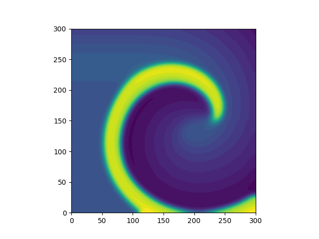
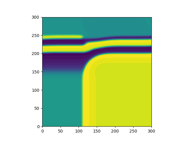
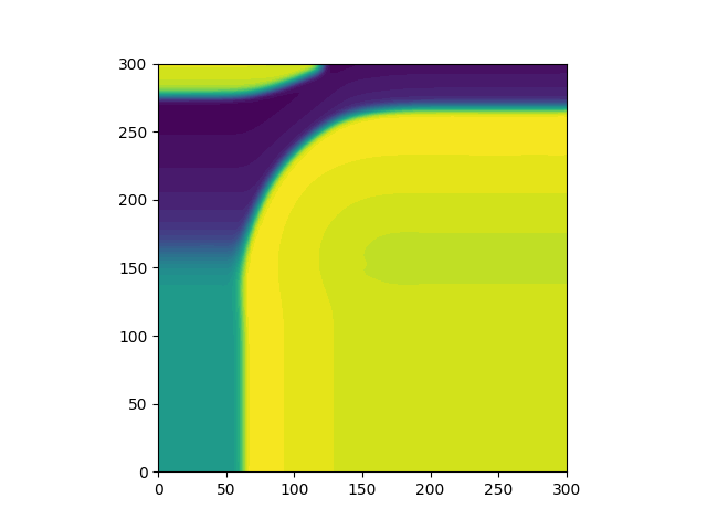
4.3 Application to Nerve Pulse Propagation
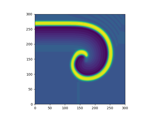
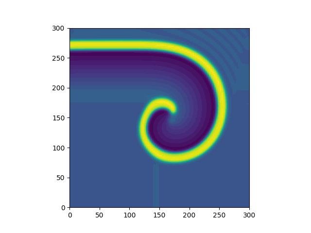
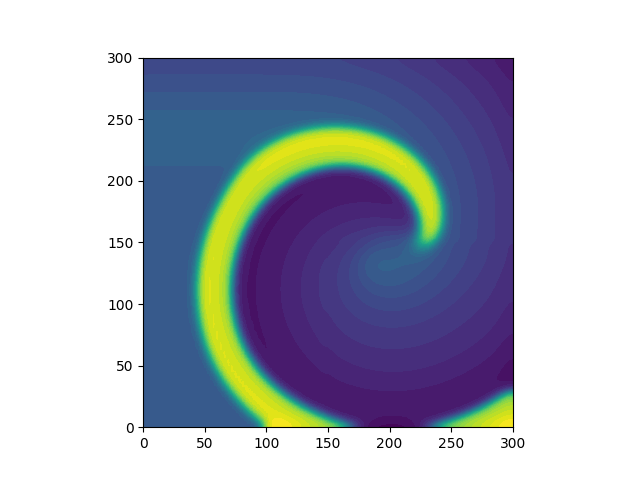
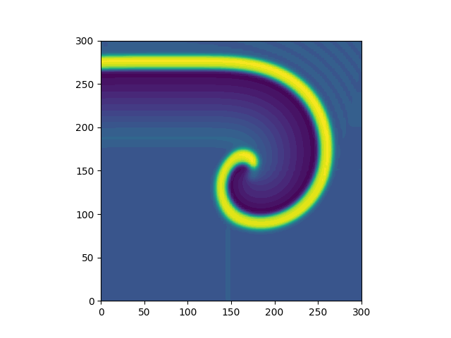
We conclude this section by showing a difference of qualitative illustration between a classical bistable equation with a weakly singular kernel (without advection, and with a simplified cubic nonlinearity induced by ) and the generalized Burgers-Huxley equation with a weakly singular kernel. In this study, we perform a straightforward simulation to a transient problem which incorporates an additional ordinary differential equation (ODE). This inclusion allows for the emergence of self-sustained patterns, as discussed in Bini et al. (2010). The system reads
| (33) |
where and are parameters that can change the rest state and dynamics. Setting , and , one recovers the well-known FitzHugh-Nagumo equations
To obtain the weak formulation similar to (21) for the CFEM, we apply a simple backward Euler time discretization with constant time step and other parameters similar to Khan et al. (2021). For this example, we prescribe Neumann boundary conditions for on . Figure 1 depicts three snapshots of the evolution of (representing the action potential propagation in a piece of nerve tissue, cardiac muscle, or any excitable media) for the classical FitzHugh-Nagumo system with weakly singular kernel vs. the modified delayed generalized Burgers-Huxley system with weakly singular kernel (4.3). All numerical solutions computed using the CFEM setting. The difference in the spiral dynamics appears to be more responsive to the degree of non-linearity (governed by ) rather than the additional advection term (influenced by ).


5 Acknowledgement
The first author would like to thank Ministry of Education, Government of India (Prime Minister Research Fellowship, PMRF ID : 2801816), for financial support to carry out his research work.
References
- Ablowitz et al. (1987) Ablowitz, M. J., Fuchssteiner, B. & Kruskal, M. (1987) Topics in soliton theory and exactly solvable nonlinear equations: proceedings of the conference on nonlinear evolution equations, solitons and the inverse scattering transform. World Scientific.
- Adolfsson et al. (2003) Adolfsson, K., Enelund, M. & Larsson, S. (2003) Adaptive discretization of an integro-differential equation with a weakly convolution kernel. Comput. Methods Appl. Mech. Engrg., 192, 5285–5304.
- Alnæs et al. (2015) Alnæs, M., Blechta, J., Hake, J., Johansson, A., Kehlet, B., Logg, A., Richardson, C., Ring, J., Rognes, M. E. & Wells, G. N. (2015) The fenics project version 1.5. Archive of Numerical Software, 3.
- Bini et al. (2010) Bini, D., Cherubini, C., Filippi, S., Gizzi, A. & Ricci, P. E. (2010) On spiral waves arising in natural systems. Commun. Comput. Phys., 8, 610–622.
- Burgers (1948) Burgers, J. M. (1948) A mathematical model illustrating the theory of turbulence. Academic Press, Inc., New York, N. Y.
- Cannon & Lin (1987) Cannon, J. & Lin, Y. (1987) A priori error estimates for galerkin method for nonlinear parabolic integro-differential equations. Manuscript.
- Cannon & Lin (1988) Cannon, J. & Lin, Y. (1988) Non-classical projection and galerkin methods for non-linear parabolic integro-differential equations. Calcolo, 25, 187–201.
- Chen et al. (1992) Chen, C., Thomée, V. & Wahlbin, L. B. (1992) Finite element approximation of a parabolic integro-differential equation with a weakly singular kernel. Math. Comp., 58, 587–602.
- Chrysafinos & Hou (2002) Chrysafinos, K. & Hou, L. S. (2002) Error estimates for semidiscrete finite element approximations of linear and semilinear parabolic equations under minimal regularity assumptions. SIAM J. Numer. Anal., 40, 282–306.
- Dautray & Lions (1990) Dautray, R. & Lions, J.-L. (1990) Mathematical analysis and numerical methods for science and technology. Vol. 4. Springer-Verlag, Berlin.
- El-Danaf (2007) El-Danaf, T. S. (2007) Solitary wave solutions for the generalized Burgers-Huxley equation. Int. J. Nonlinear Sci. Numer. Simul., 8, 315–318.
- Evans (2010) Evans, L. C. (2010) Partial differential equations. American Mathematical Soc.
- Grisvard (1985) Grisvard, P. (1985) Elliptic problems in nonsmooth domains. Pitman (Advanced Publishing Program), Boston, MA.
- Hashim et al. (2006) Hashim, I., Noorani, M. S. M. & Said Al-Hadidi, M. R. (2006) Solving the generalized Burgers-Huxley equation using the Adomian decomposition method. Math. Comput. Modelling, 43, 1404–1411.
- Hou & Zhu (2006) Hou, L. S. & Zhu, W. (2006) Error estimates under minimal regularity for single step finite element approximations of parabolic partial differential equations. Int. J. Numer. Anal. Model., 3, 504–524.
- Khan et al. (2021) Khan, A., Mohan, M. T. & Ruiz-Baier, R. (2021) Conforming, nonconforming and DG methods for the stationary generalized Burgers-Huxley equation. J. Sci. Comput., 88, 1–26.
- Khattak (2009) Khattak, A. J. (2009) A computational meshless method for the generalized Burgers’-Huxley equation. Appl. Math. Model., 33, 3718–3729.
- Kumar & Mohan (2022) Kumar, A. & Mohan, M. T. (2022) Large deviation principle for occupation measures of stochastic generalized burgers–huxley equation. Journal of Theoretical Probability, 36, 1–49.
- Kumar et al. (2011) Kumar, B. V. R., Sangwan, V., Murthy, S. V. S. S. N. V. G. K. & Nigam, M. (2011) A numerical study of singularly perturbed generalized Burgers-Huxley equation using three-step Taylor-Galerkin method. Comput. Math. Appl., 62, 776–786.
- Langtangen & Logg (2016) Langtangen, H. P. & Logg, A. (2016) Solving PDEs in Python. Springer, Cham.
- Mahajan & Khan (Prep) Mahajan, S. & Khan, A. (Prep.) Finite element approximaton for the delayed generalised Burgers- Huxley equation with weakly singular kernels: Part II Non-conforming and DG approximaton (under prepartion).
- McLean et al. (1996) McLean, W., Thomée, V. & Wahlbin, L. B. (1996) Discretization with variable time steps of an evolution equation with a positive-type memory term. J. Comput. Appl. Math., 69, 49–69.
- McLean & Mustapha (2007) McLean, W. & Mustapha, K. (2007) A second-order accurate numerical method for a fractional wave equation. Numer. Math., 105, 481–510.
- McLean & Thomée (1993) McLean, W. & Thomée, V. (1993) Numerical solution of an evolution equation with a positive-type memory term. J. Austral. Math. Soc. Ser. B, 35, 23–70.
- Mitrovic & Zubrinic (1997) Mitrovic, D. & Zubrinic, D. (1997) Fundamentals of applied functional analysis. CRC Press.
- Mohan (2020) Mohan, M. T. (2020) On the three dimensional Kelvin-Voigt fluids: global solvability, exponential stability and exact controllability of Galerkin approximations. Evol. Equ. Control Theory, 9, 301–339.
- Mohan & Khan (2021) Mohan, M. T. & Khan, A. (2021) On the generalized Burgers-Huxley equation: Existence, uniqueness, regularity, global attractors and numerical studies. Discrete Contin. Dyn. Syst. Ser. B, 26, 3943–3988.
- Mohan & Sritharan (2019) Mohan, M. T. & Sritharan, S. S. (2019) Stochastic Navier-Stokes equations perturbed by Lévy noise with hereditary viscosity. Infin. Dimens. Anal. Quantum Probab. Relat. Top., 22, 1950006.
- Mustapha & McLean (2009) Mustapha, K. & McLean, W. (2009) Discontinuous Galerkin method for an evolution equation with a memory term of positive type. Math. Comp., 78, 1975–1995.
- Mustapha & Mustapha (2010) Mustapha, K. & Mustapha, H. (2010) A second-order accurate numerical method for a semilinear integro-differential equation with a weakly singular kernel. IMA J. Numer. Anal., 30, 555–578.
- Oldham & Spanier (1974) Oldham, K. & Spanier, J. (1974) The fractional calculus theory and applications of differentiation and integration to arbitrary order. Elsevier.
- Pani & Peterson (1996) Pani, A. K. & Peterson, T. E. (1996) Finite element methods with numerical quadrature for parabolic integrodifferential equations. SIAM J. Numer. Anal., 33, 1084–1105.
- Robinson & Pierre (2003) Robinson, J. C. & Pierre, C. (2003) Infinite-dimensional dynamical systems: An introduction to dissipative parabolic pdes and the theory of global attractors. cambridge texts in applied mathematics. Appl. Mech. Rev., 56, B54–B55.
- Sari et al. (2011) Sari, M., Gurarslan, G. & Zeytinougu, A. (2011) High-order finite difference schemes for numerical solutions of the generalized Burgers-Huxley equation. Numer. Methods Partial Differential Equations, 27, 1313–1326.
- Sloan & Thomée (1986) Sloan, I. H. & Thomée, V. (1986) Time discretization of an integro-differential equation of parabolic type. SIAM J. Numer. Anal., 23, 1052–1061.
- Temam (2001) Temam, R. (2001) Navier-Stokes equations: theory and numerical analysis, vol. 343. American Mathematical Soc.
- Thomée (2007) Thomée, V. (2007) Galerkin finite element methods for parabolic problems. Springer Science & Business Media.
- Thomée & Zhang (1989) Thomée, V. & Zhang, N. Y. (1989) Error estimates for semidiscrete finite element methods for parabolic integro-differential equations. Math. Comp., 53, 121–139.
- Wang et al. (1990) Wang, X., Zhu, Z. & Lu, Y. (1990) Solitary wave solutions of the generalised Burgers-Huxley equation. Journal of Physics A: Mathematical and General, 23, 271.
- Wang (1985) Wang, X.-y. (1985) Nerve propagation and wall in liquid crystals. Physics Letters A, 112, 402–406.
- Wazwaz (2005) Wazwaz, A.-M. (2005) Travelling wave solutions of generalized forms of Burgers, Burgers–Kdv and Burgers–Huxley equations. Applied Mathematics and Computation, 169, 639–656.
- Wazwaz (2009) Wazwaz, A.-M. (2009) Burgers, fisher and related equations. Partial Differential Equations and Solitary Waves Theory. Springer, pp. 665–681.
- Yanik & Fairweather (1988) Yanik, E. G. & Fairweather, G. (1988) Finite element methods for parabolic and hyperbolic partial integro-differential equations. Nonlinear Anal., 12, 785–809.
- Yi & Guo (2015) Yi, L. & Guo, B. (2015) An - version of the continuous Petrov-Galerkin finite element method for Volterra integro-differential equations with smooth and nonsmooth kernels. SIAM J. Numer. Anal., 53, 2677–2704.
- Zhang (1993) Zhang, N. Y. (1993) On fully discrete Galerkin approximations for partial integro-differential equations of parabolic type. Math. Comp., 60, 133–166.
- Zhou et al. (2019) Zhou, J., Xu, D. & Dai, X. (2019) Weak Galerkin finite element method for the parabolic integro-differential equation with weakly singular kernel. Comput. Appl. Math., 38, Paper No. 38, 12.