Hawking Radiation Under
Generalized Uncertainty Principle

Tin-Long Chau^a , Pei-Ming Ho^a,b , Hikaru Kawai^a,b ,
Wei-Hsiang Shao^a , and Cheng-Tsung Wang^a

^aDepartment of Physics and Center for Theoretical Physics,
National Taiwan University, Taipei 10617, Taiwan
^bPhysics Division, National Center for Theoretical Sciences, Taipei 10617, Taiwan

The generalized uncertainty relation is expected to be an essential element in a theory of quantum gravity. In this work, we examine its effect on the Hawking radiation of a Schwarzschild black hole formed from collapse by incorporating a minimal uncertainty length scale into the radial coordinate of the background. This is implemented in both the ingoing Vaidya coordinates and a family of freely falling coordinates. We find that, regardless of the choice of the coordinate system, Hawking radiation is turned off at around the scrambling time. Interestingly, this phenomenon occurs while the Hawking temperature remains largely unmodified.

 

 

1 Introduction

Hawking’s seminal discovery [1, 2] of the evaporation of black holes has given rise to the information loss problem [3, 4], the resolution of which is expected to offer new insights into quantum gravity. However, the conventional description [2] of Hawking radiation within the framework of effective field theory involves trans-Planckian modes, thus leaving some room of doubt regarding the validity of its predictions [5, 6]. In particular, recent investigations [7, 8, 9, 10] have shown that the inclusion of higher-derivative (non-renormalizable) couplings between the radiation field and background curvature leads to a breakdown of the effective field theory beyond the scrambling time , owing to the genuinely high (Lorentz-invariant) energy scales of the processes involved. With that being said, there is still a widespread belief that Hawking radiation, as predicted by the low-energy effective theory, remains robust against physics in the UV regime. This idea has garnered additional support over the years through examining a variety of UV models [12, 13, 14, 15, 16, 17, 18, 19, 20, 21, 22]. Nevertheless, there are also studies that entertain the possibility of a different outcome [23, 24, 25, 26, 10, 27].

A common theme across various approaches to quantum gravity is the emergence of a fundamental minimum length scale $\ell$ [28, 29], such as the string length or the Planck length, below which the usual notion of spacetime breaks down. Since the precise quantum-gravitational effects at this scale remain unknown, in order to address the implications of a minimum length, a pragmatic approach often employed is to introduce it through the Generalized Uncertainty Principle (GUP): 

$$\Delta x\Delta p\geq\frac{1}{2}\left[1+\ell^{2}(\Delta p)^{2}\right]\,,$$ (1.1)

where $\Delta x$ and $\Delta p$ represent the uncertainties in position and momentum, respectively. This relation is motivated by string theory [30, 31, 32, 33, 34, 35, 36] as well as general considerations of quantum gravity [37, 38, 39, 40, 41], and it results in a minimal uncertainty $(\Delta x)_{\text{min}}=\ell$ in position.

In this work, we aim to study the impact of the GUP (1.1) on the Hawking radiation of a large dynamical black hole ($a\gg\ell$) with spherical symmetry. The minimum length $\ell$ is introduced into the position $x$ representing the radial coordinate of this background, which we implement by deforming the commutator in the Heisenberg algebra as [42, 43, 44] 

$$\left[\hat{x},\hat{p}\right]=i\left(1+\ell^{2}\hat{p}^{2}\right)\,.$$ (1.2)

This modification can be realized in momentum space via the representation [42]

$$\hat{x}\equiv i\left(1+\ell^{2}p^{2}\right)\partial_{p}\,,\qquad\hat{p}=p\,.$$ (1.3)

Within this framework, the corrections induced by the GUP are encoded in the wave equation governing the radiation field, leading to significant alterations of the behavior of Hawking modes that probe the black hole background with trans-Planckian momenta.

This GUP framework has been previously applied [47] to investigate Hawking radiation in the Eddington-Finkelstein coordinates, revealing intriguing effects on wave packet propagation. Furthermore, there are extensive studies in the literature on corrections to the Unruh temperature [48], Hawking temperature, and other thermodynamic properties of black holes within the context of GUP [49, 50, 51, 52, 53, 54, 55, 56, 57, 58, 59, 60, 61, 62, 63, 64, 65, 66, 67, 68, 69]. In contrast, in this work we shall focus on the time-dependent magnitude of Hawking radiation. Notably, we discover that Hawking radiation maintains a thermal spectrum

$$\expectationvalue{\mathcal{N}_{\omega}(t)}\approx\frac{1}{e^{\omega/T_{H}}-1}\,\mathcal{A}(t)$$ (1.4)

characterized by essentially the same Hawking temperature $T_{H}=1/4\pi a$, but with an amplitude $\mathcal{A}(t)$ that diminishes significantly after the scrambling time: 

$$\mathcal{A}(t)\to 0\quad\text{for}\quad t\gtrsim 2a\log(a/\ell)\,,$$ (1.5)

where $t$ denotes the duration in Schwarzschild time, starting from the moment the collapsing matter is at a distance of $\mathcal{O}(a)$ from the black hole horizon.

The suppression of Hawking radiation at late times can be attributed to the substantial change in the behavior of $\Delta x$ in the domain of large $\Delta p\gtrsim\ell^{-1}$ caused by the GUP (1.1). In the low-energy effective theory which assumes locality and a reciprocal relation between the uncertainties $\Delta x$ and $\Delta p$, an outgoing wave packet with purely positive frequency at a large distance can be traced back in time to the near-horizon region, where the central momentum of the wave packet experiences an exponential blueshift. This causes the packet to be densely compressed close to the horizon in the past with $\Delta x\lesssim\ell$. Consequently, the wave packet has a broad spectrum $\Delta p$ in momentum, consisting of both positive and negative-$p$ components. This mixture is the key ingredient for the production of Hawking radiation.

In the case of the GUP (1.1), however, a remarkable observation is that in fact $\Delta x\gg a$ due to the immensely large spread in momentum $\Delta p\gg a/\ell^{2}$ when the wave packet is traced back to a distance of $\mathcal{O}(\ell)$ from the horizon. Not only does this imply that the wave packet is no longer confined within the near-horizon region, it also suggests that the wave packet might even largely surpass the size of the black hole itself, to the extent where its evolution is insensitive to the black hole spacetime. As a result, modes with trans-Planckian momenta do not contribute to Hawking radiation, leading to the termination of radiation after the scrambling time.

This paper is organized as follows. In Sec. 2, we incorporate the GUP into the free field theory in the ingoing Vaidya spacetime. This is achieved by formulating the theory in momentum space and employing the representation (1.3). We find that Hawking radiation is turned off after the scrambling time, as defined in eq. (1.5). In Sec. 3, we extend our analysis by introducing the GUP into a family of freely falling coordinates. Although the implementation of the GUP (1.1) depends on the choice of the reference frame, we arrive at the same conclusion regarding the late-time suppression of Hawking radiation. Finally, we wrap up the discussion with a summary and concluding remarks in Sec. 4.

2 GUP in Vaidya Coordinates

In this section, we adopt the approach outlined in Ref. [47] to study how Hawking radiation is affected by the GUP defined with respect to the ingoing Vaidya coordinates. Our findings indicate that the incorporation of GUP leads to the termination of Hawking radiation beyond the scrambling time.

Let us begin our discussion by establishing the setup of the problem. Recall that a four-dimensional spherically-symmetric black hole with Schwarzschild radius $a$ can be described by the metric 

$$ds^{2}=-\left(1-\frac{a}{r}\right)dt^{2}+\left(1-\frac{a}{r}\right)^{-1}dr^{2}+r^{2}d\Omega^{2}\,,$$ (2.1)

where $d\Omega^{2}$ stands for the differential solid angle on a unit 2-sphere. Through a coordinate transformation, this metric can be expressed as

$$ds^{2}=-\left(1-\frac{a}{r}\right)dv^{2}+2dvdr+r^{2}d\Omega^{2}$$ (2.2)

in terms of the Eddington-Finkelstein coordinates, where $v(t,r)\equiv t+r_{*}$ and the tortoise coordinate $r_{*}$ is defined by

$$r_{\ast}\equiv r+a\log\left(\frac{r}{a}-1\right)\,.$$ (2.3)

Outgoing waves travelling at the speed of light are purely functions of the Eddington retarded time $u(t,r)\equiv t-r_{*}$.

We consider a simple model where the black hole is formed from a thin shell of spherical matter collapsing at the speed of light. It is then natural to describe the geometry using the ingoing Vaidya metric

$$ds^{2}=-\left(1-\Theta(v)\,\frac{a}{r}\right)dv^{2}+2dvdr\,,$$ (2.4)

where $\Theta(v)$ represents the step function, and for simplicity, we have omitted the angular part of the metric. Without loss of generality, we have assumed that the trajectory of the infalling null shell is given by $v=0$. Outside the shell ($v>0$), the metric corresponds to the Schwarzschild metric, with the event horizon located at $r=a$. In the region inside the shell ($v<0$), the geometry is that of Minkowski space.

In the near-horizon region of the Vaidya background where

$$x\equiv r-a\ll a\,,$$ (2.5)

the action for a massless real scalar field in the low-energy effective theory is given by

$$S_{0}=-\frac{1}{2}\int dv\int dx\left[\partial_{x}\phi(v,x)\right]\biggl{\{}2\partial_{v}+\left[1+\Theta(v)\left(\frac{x}{a}-1\right)\right]\partial_{x}\biggr{\}}\phi(v,x)\,.$$ (2.6)

Via the Fourier transform

$$\phi(v,x)=\int_{-\infty}^{\infty}\frac{dp}{\sqrt{2\pi}}\,\tilde{\phi}(v,p)\,e^{ipx}\,,$$ (2.7)

the action (2.6) is equivalent to

$$S_{0} =\int dv\left\langle\tilde{\phi}(v,p)\left|\,p\left[i\partial_{v}-\frac{p}{2}-\Theta(v)\left(\frac{\hat{x}}{2a}\,p-\frac{p}{2}\right)\right]\right|\tilde{\phi}(v,p)\right\rangle_{0}\,,$$ (2.8)

where $\hat{x}\equiv i\partial_{p}$ and the definition of $\langle A\,|\,\mathopen{}B\rangle_{0}$ is

$$\langle A\,|\,\mathopen{}B\rangle_{0}\equiv\int_{-\infty}^{\infty}dp\,A^{*}(p)B(p)\,.$$ (2.9)

Note that the relativistic inner product conserved under time evolution is $\langle\tilde{\phi}_{1}|\,p\,|\tilde{\phi}_{2}\rangle_{0}$.

To accommodate the GUP in this setup, we shall utilize the momentum-space representation (see for example Refs. [71, 13]) and, without loss of generality, realize the modified commutator algebra (1.2) by adopting eq. (1.3). It then follows that eq. (2.9) should also be modified as

$$\left\langle A\,\middle|\,\mathopen{}B\right\rangle\equiv\int_{-\infty}^{\infty}\frac{dp}{1+\ell^{2}p^{2}}\,A^{*}(p)B(p)\,,$$ (2.10)

where a measure factor $1/(1+\ell^{2}p^{2})$ has been introduced to ensure the Hermiticity of $\hat{x}$ (1.3) on the domain of functions that decay at $\pm\infty$ [42].

Following Ref. [47], the GUP modification of the action (2.8) for a massless real scalar is obtained by employing the representation (1.3) and also replacing $\langle A\,|\,\mathopen{}B\rangle_{0}$ in the action with $\langle A\,|\,\mathopen{}B\rangle$ as defined in eq. (2.10), incorporating the appropriate measure factor. This results in

$$S_{\mathrm{GUP}} =\int dv\int_{-\infty}^{\infty}\frac{dp}{1+\ell^{2}p^{2}}\,\tilde{\phi}^{\ast}(v,p)\,p\left[i\partial_{v}-\frac{p}{2}-\Theta(v)\left(\frac{\hat{x}}{2a}\,p-\frac{p}{2}\right)\right]\tilde{\phi}(v,p)$$

$$=2\int dv\int_{0}^{\infty}\frac{dp}{1+\ell^{2}p^{2}}\,\tilde{\phi}^{\ast}(v,p)\,p\left\{i\partial_{v}-\frac{p}{2}-\Theta(v)\left[\frac{i(1+\ell^{2}p^{2})}{2a}\,\partial_{p}\,p-\frac{p}{2}\right]\right\}\tilde{\phi}(v,p)\,,$$ (2.11)

where in the second line we performed a partial integration and then imposed the reality condition

$$\tilde{\phi}^{\ast}(v,p)=\tilde{\phi}(v,-p)$$ (2.12)

on the real scalar field. Variation of the action (2.11) leads to the field equation

$$\left\{i\partial_{v}-\frac{p}{2}-\Theta(v)\left[\frac{i\left(1+\ell^{2}p^{2}\right)}{2a}\,\partial_{p}\,p-\frac{p}{2}\right]\right\}\tilde{\phi}(v,p)=0\,,$$ (2.13)

which demands the continuity of $\tilde{\phi}(v,p)$ across the null shell at $v=0$. According to the field equation, the $v$-derivative of the relativistic inner product of any two solutions $\tilde{\phi}_{1}$ and $\tilde{\phi}_{2}$ is

$$\partial_{v}\langle\tilde{\phi}_{1}(v)|\,p\,|\tilde{\phi}_{2}(v)\rangle =\frac{\Theta(v)}{2a}\,\Bigl{[}p^{2}\,\tilde{\phi}_{1}^{*}(v,p)\,\tilde{\phi}_{2}(v,p)\Bigr{]}\Big{|}^{\infty}_{p\,=\,-\infty}\,.$$ (2.14)

Hence, the inner product is conserved under time evolution for solutions satisfying the boundary condition

$$\lim_{p\rightarrow\pm\infty}p\,\tilde{\phi}(v,p)=0\,.$$ (2.15)

Now let us consider the general solution to the field equation (2.13) inside and outside the shell, respectively. In the flat spacetime inside the collapsing shell ($v<0$), the equation is simply

$$\left(i\partial_{v}-\frac{p}{2}\right)\tilde{\phi}(v,p)=0\,,$$ (2.16)

and its general solution can be written as

$$\tilde{\phi}(v<0,p)=e^{-ipv/2}\sqrt{\frac{1+\ell^{2}p^{2}}{2|p|}}\left[a_{p}\,\Theta(p)+a_{-p}^{\dagger}\,\Theta(-p)\right]\,.$$ (2.17)

Upon quantization, where the field $\tilde{\phi}$ and its conjugate momentum

$$\widetilde{\Pi}(v,p)=\frac{2ip}{1+\ell^{2}p^{2}}\,\tilde{\phi}^{\ast}(v,p)$$ (2.18)

are promoted to operators satisfying the equal-time commutation relation $\commutator*{\tilde{\phi}(v,p)}{\widetilde{\Pi}(v,p^{\prime})}=i\,\delta(p-p^{\prime})$, the creation and annihilation operators obey

$$\commutator*{a_{p}}{a_{p^{\prime}}^{\dagger}}=\delta(p-p^{\prime})\,,\qquad\commutator{a_{p}}{a_{p^{\prime}}}=0\,,\qquad\commutator*{a_{p}^{\dagger}}{a_{p^{\prime}}^{\dagger}}=0\,.$$ (2.19)

The quantum state of the field $\phi$ inside the shell is assumed to be the Minkowski vacuum $\ket{0}$ defined by

$$\ket{0}\;\ni\;a_{p}\ket{0}=0\quad\forall\,p>0\,.$$ (2.20)

In the Schwarzschild spacetime outside the shell ($v>0$), the field equation (2.13) takes the form

$$\left[\partial_{v}-\frac{(1+\ell^{2}p^{2})}{2a}\,\partial_{p}\,p\right]\tilde{\phi}(v,p)=0\,,$$ (2.21)

and its general solution is given by

$$\tilde{\phi}(v>0,p)=p^{-1}\,\Psi\bigl{(}v+2aF(p)\bigr{)}$$ (2.22)

for an arbitrary function $\Psi$, where

$$F(p)\equiv\log\left(\frac{a\absolutevalue{p}}{\sqrt{1+\ell^{2}p^{2}}}\right)\,.$$ (2.23)

A special case is the single-frequency solution describing a Hawking mode:

$$\tilde{\phi}_{\omega}(v,p)=\mathcal{N}_{\omega}\,\frac{e^{-i\omega v}}{p-i0^{+}}\left[\frac{a\left(p-i0^{+}\right)}{\sqrt{1+\ell^{2}p^{2}}}\right]^{-2ia\omega}\,,$$ (2.24)

where $\omega$ is the Killing frequency with respect to the advanced time coordinate $v$, and $\mathcal{N}_{\omega}$ is an overall constant that will be fixed shortly. The prescription $p\to p-i0^{+}$ for analytic continuation is introduced so that $\tilde{\phi}_{\omega}(v,p)$ corresponds to an outgoing wave outside the horizon [71] (see also Ref. [27]).

Given the characteristic trajectory

$$v+2aF(p)=\text{constant}$$ (2.25)

inferred from the general solution (2.22), it is evident that at sufficiently large values of $v$, the prevailing momentum is very sub-Planckian, i.e., $\absolutevalue{p}\ll\ell^{-1}$, and it is thus reasonable to treat $\ell p\to 0$ in this regime. As a result, a typical Hawking mode (2.24) with frequency $\omega\sim 1/a\ll\ell^{-1}$ essentially evolves in accordance with the low-energy effective theory at large $v$, and is expected to coincide with the outgoing plane wave $e^{-i\omega u}/\sqrt{2\omega}\approx e^{-i\omega v}\left(x/a\right)^{2ia\omega}/\sqrt{2\omega}$. It is then natural to choose the normalization constant $\mathcal{N}_{\omega}$ such that [47]

$$\phi_{\omega}(v,x)\approx\mathcal{N}_{\omega}\,\int_{-\infty}^{\infty}\frac{dp}{\sqrt{2\pi}}\,e^{ipx}\,\frac{e^{-i\omega v}}{p-i0^{+}}\left[a(p-i0^{+})\right]^{-2ia\omega}=\frac{e^{-i\omega v}}{\sqrt{2\omega}}\left(\frac{x}{a}\right)^{2ia\omega}\,,$$ (2.26)

where $\phi_{\omega}(v,x)$ is related to $\tilde{\phi}_{\omega}(v,p)$ via the Fourier transform (2.7). Since $\mathcal{N}_{\omega}$ is independent of both $p$ and $v$, it can be uniquely fixed by this equation to be

$$\mathcal{N}_{\omega}\approx a\sqrt{\frac{\omega}{\pi}}\,e^{\pi a\omega}\,\Gamma(2ia\omega)\quad\mbox{for}\quad\omega\ll\ell^{-1}\,,$$ (2.27)

which leads to

$$\left|\mathcal{N}_{\omega}\right|^{2}\approx\frac{a}{1-e^{-4\pi a\omega}}\,.$$ (2.28)

In order to capture the time dependence of Hawking radiation, we consider a localized Hawking particle with a wave function represented by an outgoing wave packet constructed as a superposition of the monochromatic solutions (2.24):

$$\widetilde{\Psi}_{(\omega_{0},u_{0})}(v,p)=\int_{0}^{\infty}d\omega\,f_{\omega_{0}}(\omega)\,e^{i\omega u_{0}}\,\tilde{\phi}_{\omega}(v,p)\,.$$ (2.29)

This packet has central frequency $\omega_{0}$ and is centered around a given Eddington retarded time $u=u_{0}$. The profile function $f_{\omega_{0}}(\omega)$ is assumed to possess a narrow width $\Delta\omega$ such that $|f_{\omega_{0}}(\omega)|$ is negligible when $|\omega-\omega_{0}|\gg\Delta\omega$ . Moreover, $f_{\omega_{0}}(\omega)$ is suitably normalized so that

$$\int_{0}^{\infty}d\omega\,\absolutevalue{f_{\omega_{0}}(\omega)}^{2}=1\,.$$ (2.30)

To better understand the wave packet construction (2.29), recall that at large values of $v$, the effects of the GUP can be neglected due to the dominant momentum being small ($\ell p\ll 1$). Consequently, the mode solutions $\phi_{\omega}$ in the superposition can be approximated by outgoing plane waves as demonstrated in eq. (2.26), and the position-space representation of the wave packet (2.29) can be simplified as

$$\int_{-\infty}^{\infty}\frac{dp}{\sqrt{2\pi}}\,e^{ipx}\,\widetilde{\Psi}_{(\omega_{0},u_{0})}(v\gg u_{0}\,,p)\approx\frac{1}{\sqrt{2\omega_{0}}}\int_{0}^{\infty}d\omega\,f_{\omega_{0}}(\omega)\,e^{-i\omega(u-u_{0})}\equiv\Psi_{\omega_{0}}(u-u_{0})\,.$$ (2.31)

The term $1/\sqrt{2\omega}$ is treated as a slowly-varying factor, which allows us to approximate it by a constant in the frequency domain where $f_{\omega_{0}}(\omega)$ has support. By definition, $\Psi_{\omega_{0}}(u)$ describes a null wave (hence a function of $u$ only) centered around $u=0$. Therefore, $\Psi_{\omega_{0}}(u-u_{0})$ is an outgoing wave packet localized around $u=u_{0}$ with a width of $\Delta u\sim 1/\Delta\omega$ in the $u$-space. Substituting the solution (2.24) into eq. (2.29) explicitly, we obtain

$$\widetilde{\Psi}_{(\omega_{0},u_{0})}(v,p) =\int_{0}^{\infty}d\omega\,f_{\omega_{0}}(\omega)\,e^{i\omega u_{0}}\,\mathcal{N}_{\omega}\,\frac{e^{-i\omega v}}{p-i0^{+}}\left[\frac{a\left(p-i0^{+}\right)}{\sqrt{1+\ell^{2}p^{2}}}\right]^{-2ia\omega}$$

$$\approx\sqrt{2\omega_{0}}\,\mathcal{N}_{\omega_{0}}\,\frac{e^{-2\pi a\omega_{0}\Theta(-p)}}{p-i0^{+}}\,\Psi_{\omega_{0}}\bigr{(}v+2aF(p)-u_{0}\bigr{)}\,,$$ (2.32)

where the slowly-varying factors have again been treated as constants and pulled out of the $\omega$-integral.

We can associate to the Hawking particle corresponding to the wave packet (2.29) an annihilation operator $b_{\Psi}$ defined as the relativistic inner product between $\widetilde{\Psi}_{(\omega_{0},u_{0})}$ and the field operator $\tilde{\phi}$, i.e.

$$b_{\Psi}\equiv\bigl{\langle}\widetilde{\Psi}_{(\omega_{0},u_{0})}\bigl{|}\,p\,\bigr{|}\tilde{\phi}\bigr{\rangle}\,.$$ (2.33)

The number expectation value of Hawking particles with the wave function $\widetilde{\Psi}_{(\omega_{0},u_{0})}$ in the Minkowski vacuum $|0\rangle$ (2.20) is then determined by how the operator $b_{\Psi}$ is decomposed in terms of the creation and annihilation operators $\{a_{p},a_{p}^{\dagger}\}$ inside the shell. According to eq. (2.17), this is equivalent to a decomposition into positive and negative-$p$ components. The calculation of Hawking radiation thus amounts to tracing the wave packet $\widetilde{\Psi}_{(\omega_{0},u_{0})}$ back in time to the collapsing shell at $v=0$, where the field $\tilde{\phi}$ can be matched with the mode expansion (2.17) inside the shell. After that, we evaluate the norm of the negative-momentum components present in the wave packet. More explicitly, using the definition in eq. (2.10), we have

$$b_{\Psi} =\bigl{\langle}\widetilde{\Psi}_{(\omega_{0},u_{0})}(v=0)\bigl{|}\,p\,\bigr{|}\tilde{\phi}(v=0)\bigr{\rangle}$$

$$=\int_{0}^{\infty}dp\,\sqrt{\frac{p}{2\left(1+\ell^{2}p^{2}\right)}}\left[\widetilde{\Psi}_{(\omega_{0},u_{0})}^{*}(0,p)\,a_{p}-\widetilde{\Psi}_{(\omega_{0},u_{0})}^{*}(0,-p)\,a_{p}^{\dagger}\right]\,,$$ (2.34)

thus the vacuum expectation value of the number of Hawking particles is

$$\expectationvalue{b_{\Psi}^{\dagger}b_{\Psi}}{0} =\int_{0}^{\infty}dp\,\frac{p}{2(1+\ell^{2}p^{2})}\,\absolutevalue\big{\widetilde{\Psi}_{(\omega_{0},u_{0})}(0,-p)}^{2}$$

$$=\frac{1}{2}\,\Bigl{\langle}\Theta(p)\,\widetilde{\Psi}_{(\omega_{0},u_{0})}(0,-p)\Bigl{|}\,p\,\Bigr{|}\Theta(p)\,\widetilde{\Psi}_{(\omega_{0},u_{0})}(0,-p)\Bigr{\rangle}\,,$$ (2.35)

which is indeed determined by the norm of the negative-momentum components in the wave packet $\widetilde{\Psi}_{(\omega_{0},u_{0})}$.

To evaluate eq. (2.35), we first derive the identity

$$\bigl{\langle}\Theta(p)\,\tilde{\phi}_{\omega}(0,-p)\bigl{|}\,p\,\bigr{|}\Theta(p)\,\tilde{\phi}_{\omega^{\prime}}(0,-p)\bigr{\rangle}$$

$$= \int_{0}^{\infty}\frac{dp}{1+\ell^{2}p^{2}}\,\tilde{\phi}_{\omega}^{*}(0,-p)\,p\,\tilde{\phi}_{\omega^{\prime}}(0,-p)$$

$$= \ \mathcal{N}_{\omega}^{*}\,\mathcal{N}_{\omega^{\prime}}\,e^{-2\pi a(\omega\,+\,\omega^{\prime})}\int_{0}^{\infty}\frac{dp}{p\left(1+\ell^{2}p^{2}\right)}\,\exp\left[2ia(\omega-\omega^{\prime})\log\left(\frac{ap}{\sqrt{1+\ell^{2}p^{2}}}\right)\right]$$

$$= \ \mathcal{N}_{\omega}^{*}\,\mathcal{N}_{\omega^{\prime}}\,e^{-2\pi a(\omega\,+\,\omega^{\prime})}\int_{-\infty}^{\log(a/\ell)}dF\,e^{2ia(\omega-\omega^{\prime})F}$$ (2.36)

by plugging in the mode solutions (2.24) and making a change of variables from $p$ to $F(p)$ as introduced in eq. (2.23). We observe that the influence of the GUP emerges in the form of an upper bound $\log(a/\ell)$ on the $F$-integration. Finally, by substituting eq. (2.36) into eq. (2.35) and making use of eq. (2.28), we find the number of Hawking particles with the wave function $\widetilde{\Psi}_{(\omega_{0},u_{0})}$ in Hawking radiation to be

$$\expectationvalue{b_{\Psi}^{\dagger}b_{\Psi}}{0} \approx\frac{a}{2}\,\frac{e^{-4\pi a\omega_{0}}}{1-e^{-4\pi a\omega_{0}}}\int d\omega\,f_{\omega_{0}}^{*}(\omega)\int d\omega^{\prime}\,f_{\omega_{0}}(\omega^{\prime})\,e^{-i(\omega-\omega^{\prime})u_{0}}\int_{-\infty}^{\log(a/\ell)}dF\,e^{2ia(\omega-\omega^{\prime})F}$$

$$=\frac{1}{4}\,\frac{1}{e^{4\pi a\omega_{0}}-1}\int d\omega\,f_{\omega_{0}}^{*}(\omega)\int d\omega^{\prime}\,f_{\omega_{0}}(\omega^{\prime})\int_{-\infty}^{2a\log(a/\ell)-u_{0}}du\,e^{i(\omega-\omega^{\prime})u}$$

$$=\frac{1}{2}\,\frac{\omega_{0}}{e^{4\pi a\omega_{0}}-1}\times\int_{-\infty}^{2a\log(a/\ell)-u_{0}}du\,\bigl{|}\Psi_{\omega_{0}}(u)\bigr{|}^{2}\,.$$ (2.37)

It is evident from the Planck distribution factor in the spectrum that the Hawking temperature $T_{H}=1/4\pi a$ is robust. It is closely related to the analytic continuation of the term $(p-i0^{+})^{-2ia\omega}$ in the expression (2.24) for the Hawking modes across $p=0$, highlighting its significance as an infrared property.

Given that the wave function $\Psi_{\omega_{0}}(u)$ defined in eq. (2.31) is centered around $u=0$ with a width of $\Delta u$, the integral in eq. (2.37) is highly suppressed when

$$u_{0}-2a\log(a/\ell)\gtrsim\Delta u\,.$$ (2.38)

For a large black hole, the scrambling time $2a\log(a/\ell)$ is much larger than $\Delta u$, which is typically of $\mathcal{O}(a)$.. Hence, eq. (2.37) indicates that the probability of detecting Hawking particles centered around the retarded time $u_{0}$ diminishes with increasing $u_{0}$. This probability eventually tends to zero when

$$u_{0}\gtrsim 2a\log(a/\ell)\,,$$ (2.39)

signifying that Hawking radiation is turned off at around the scrambling time. Although we have essentially followed the formulation presented in Ref. [47], an explicit calculation of the time-dependent amplitude of Hawking radiation has led to a different conclusion, namely, that the GUP eventually shuts down Hawking radiation.

The origin of the termination of Hawking radiation is the non-conservation of the inner product $\langle\tilde{\phi}_{\omega}(v)|\,p\,|\tilde{\phi}_{\omega^{\prime}}(v)\rangle$ for the mode solutions (2.24), which in fact do not satisfy the boundary condition (2.15). This was already pointed out in Ref. [47], which also provided a physical interpretation of the non-conservation of the inner product as follows. In string theory, when the energy and momentum are trans-Planckian, there is a plethora of massive modes that the massless field can transition into, and the nonlocality introduced by the GUP implies the dissipation of a Hawking particle into a “reservoir” containing these massive modes when traced backward in time [47]. Here we offer a similar but slightly different interpretation, especially regarding the ultimate outcome of Hawking radiation. In our view, the trans-Planckian modes with $p\gg a/\ell^{2}$ correspond to long strings with spatial extensions $\Delta x\gg a$. Hence, they are essentially evolving in the asymptotically flat region rather than the near-horizon region, and they end up not contributing to Hawking radiation. We will elaborate more on this in the ensuing discussion.

In deriving the action (2.11) for the scalar field in the near-horizon region, we have made the assumption that $x$ is small, as indicated in eq. (2.5). This allowed us to perform a Taylor expansion of the metric up to first order in $x/a$ around $x=0$. Subsequently, we replaced $x$ with $\hat{x}=i(1+\ell^{2}p^{2})\partial_{p}$ to incorporate the effects of the GUP. Strictly speaking, this approach is not entirely self-consistent, since $\hat{x}$ becomes large as $p$ increases due to the presence of the factor $(1+\ell^{2}p^{2})$. On the other hand, the momentum $p$ experiences a significant blueshift only if $x$ is small. In Appendix A, we address this concern by repeating the calculation using the exact ingoing Vaidya metric (2.4) without relying on the assumption that $x$ is small. Remarkably, our analysis in the appendix leads to the same conclusion, affirming the validity of our findings.

Let us now discuss the physical picture behind the termination of Hawking radiation. Hawking radiation stems from the distinction between the notion of particles and vacua defined for freely falling observers in the near-horizon region ($x\ll a$) and distant observers in the asymptotically flat region ($x\gg a$). In the low-energy effective theory, since the Killing vector $\hat{P}_{u}\equiv i\partial_{u}$ and the Kruskal time-derivative operator $\hat{P}_{U}\equiv i\partial_{U}=e^{u/2a}\hat{P}_{u}$ satisfy the commutator $\commutator*{\hat{P}_{u}}{\hat{P}_{U}}=i\hat{P}_{U}/2a$, there is an uncertainty relation [9]

$$\Delta\omega\Delta\Omega\geq\frac{\langle\omega\rangle}{4a}\,e^{u/2a}$$ (2.40)

involving their associated frequencies $\omega$ and $\Omega$. As the momentum $p=2e\Omega\sim\Omega$ is related to the Kruskal frequency $\Omega$ by a constant factor of order 1 on the collapsing shell near the horizon, the inequality above implies that a Hawking wave packet with dominant frequency $\langle\omega\rangle\sim 1/a\gtrsim\Delta\omega$ detected at a later time (larger $u$) by a distant observer has a broader distribution of momentum in the past:

$$\Delta p\gtrsim\langle\omega\rangle\,e^{u/2a}\sim\langle p\rangle\,,$$ (2.41)

larger than the exponentially blueshifted value $\langle p\rangle$ itself. This ensures a mixture of positive and negative-$p$ components within a Hawking particle composed of purely positive-$\omega$ modes. More importantly, since the size $\Delta x\sim 1/\Delta p$ of the wave packet shrinks exponentially into the past in the low-energy effective theory, it can always be traced back to the near-horizon region where the notion of vacuum is different, giving rise to Hawking radiation (see eq. (2.35)).

On the other hand, when the GUP (1.1) is introduced, the uncertainty in position also grows as the momentum increases. More precisely, the GUP implies that

$$\Delta x\gg a\quad\mbox{when}\quad\Delta p\gg\frac{a}{\ell^{2}}\,.$$ (2.42)

As a consequence, for Hawking radiation beyond the scrambling time $u\gtrsim 2a\log(a^{2}/\ell^{2})$, the wave packet has a width of $\Delta p\gtrsim\langle p\rangle\sim a/\ell^{2}$ in the past, and thus spreads over a large spatial distance, encompassing mainly the asymptotically flat region. Moreover, compared to the exponential blueshift in the low-energy effective theory, the characteristic trajectory $v+2aF(p)=u_{0}$ (2.25) indicates a substantially more rapid growth in momentum during the backward propagation. In fact, Hawking particles that reach the asymptotic region after the scrambling time would have originated within the collapsing shell with a central momentum $\langle p\rangle\gg a/\ell^{2}$ far exceeding the Planck scale . Therefore, their corresponding wave packets would have spanned an extent $\Delta x\gg\mathcal{O}(a)$ far beyond the size of the black hole in the past. For these modes, the notion of vacuum naturally aligns with the vacuum for distant observers, rather than the $a_{p}$-vacuum (2.20) inside the shell. This situation remains essentially the same as these highly trans-Planckian, large-scale modes traverse through the black hole spacetime. Hence, these modes are not expected to contribute to particle creation, and this is the underlying reason why Hawking radiation comes to a stop past the scrambling time.

3 GUP in Freely Falling Frames

As the implementation of the GUP via eq. (1.3) breaks local Lorentz symmetry, it depends on the choice of the coordinate system. In this section, we extend our discussions to a class of freely falling frames. We find that, from the viewpoint of a stationary observer at a fixed distance from the horizon, the conclusion remains the same that Hawking radiation is turned off when

$$\Delta t\gtrsim 2a\log(a/\ell)\,,$$ (3.1)

where $\Delta t$ is the duration in Schwarzschild time starting from the moment when the collapsing matter is at a distance of $\mathcal{O}(a)$ from the horizon.

A particular freely falling frame was considered in previous works such as Refs. [12, 15] for the study of Hawking radiation with modified dispersion relations. It is given by the Schwarzschild metric (2.1) in the Painlevé-Gullstrand coordinates $(\tau,r)$:

$$ds^{2}=-d\tau^{2}+\left(dx+\sqrt{\frac{a}{r}}\,d\tau\right)^{2}\,,$$ (3.2)

where

$$\tau \equiv t+2\sqrt{ar}-a\log\left|\frac{\sqrt{r}+\sqrt{a}}{\sqrt{r}-\sqrt{a}}\right|\,,$$ (3.3)

$$x \equiv r-a\,.$$ (3.4)

The coordinate $\tau$ agrees with the proper time of a free falling observer following the trajectory $dx/d\tau=-\sqrt{a/r}$.

We generalize this freely falling frame as follows. Consider now a generic freely falling observer who travels radially inward along a timelike geodesic in the Schwarzschild spacetime. In terms of the Schwarzschild coordinates $(t,r)$, the geodesic equations are

$$\frac{dt}{d\tau}=\frac{E}{1-a/r}\,,\qquad\left(\frac{dr}{d\tau}\right)^{2}=E^{2}-1+\frac{a}{r}\,,$$ (3.5)

where $\tau$ is the proper time along the trajectory, and $E$ is the conserved energy per unit mass. For a geodesic that originates from the infinite past ($t\rightarrow-\infty,r\rightarrow\infty$) with an initial speed given by

$$\lim_{t\rightarrow-\infty}\left(\frac{dr}{dt}\right)^{2}=1-\gamma\,,\qquad\text{where}\ \gamma\in(0,1]\,,$$ (3.6)

we have $E=\gamma^{-1/2}$. This gives a family of freely falling trajectories $\bigl{(}t(\tau;\gamma),r(\tau;\gamma)\bigr{)}$ parametrized by $\gamma$. The case where $\gamma=1$ coincides with the special case (3.2) mentioned above, which corresponds to an observer initially at rest at past infinity. On the other hand, the limit $\gamma\to 0$ is closely related to the coordinate system considered in the previous section.

From the geodesic equations (3.5), one can introduce the proper time coordinate $\tau(t,r)$ as

$$\tau(t,r)=\gamma^{-1/2}\left[t+h_{\gamma}(r)\right]\,,$$ (3.7)

where

$$h_{\gamma}(r) \equiv\int^{r}dr^{\prime}\,\frac{\sqrt{1-\gamma(1-a/r^{\prime})}}{1-a/r^{\prime}}$$

$$\begin{split}&=\sqrt{1-\gamma(1-a/r)}\,r+\frac{(2-\gamma)}{2\sqrt{1-\gamma}}\,a\log\left\lvert\frac{\sqrt{1-\gamma}+\sqrt{1-\gamma(1-a/r)}}{\sqrt{1-\gamma}-\sqrt{1-\gamma(1-a/r)}}\right\rvert\\ &\quad-a\log\left\lvert\frac{1+\sqrt{1-\gamma(1-a/r)}}{1-\sqrt{1-\gamma(1-a/r)}}\right\rvert\end{split}$$ (3.8)

up to an irrelevant additive constant. Subsequently, eq. (3.7) can be used to define a class of free-fall coordinates $(\tau,r)$, in which the Schwarzschild line element (2.1) can be expressed as

$$ds^{2}=-d\tau^{2}+\gamma\bigl{(}dr-v_{\gamma}(r)\,d\tau\bigr{)}^{2}\,,$$ (3.9)

where

$$v_{\gamma}(r)=-\gamma^{-1/2}\sqrt{1-\gamma\left(1-\frac{a}{r}\right)}\,.$$ (3.10)

In the near-horizon region where $0<x\ll a$, we have

$$d\tau\approx\gamma^{-1/2}\left(dt+dr_{\ast}\right)=\gamma^{-1/2}dv\,.$$ (3.11)

Therefore, through a constant shift of the coordinate $\tau$, we can approximately identify $\tau$ with $\gamma^{-1/2}v$ in the near-horizon region.

In this coordinate system, the low-energy free field theory for a massless scalar has the action

$$S_{0}=\frac{\gamma^{1/2}}{2}\int d\tau\int dr\left\{\left[\left(\partial_{\tau}+v_{\gamma}(r)\,\partial_{r}\right)\phi\right]^{2}-\gamma^{-1}\left(\partial_{r}\,\phi\right)^{2}\right\}\,.$$ (3.12)

In the near-horizon region $\absolutevalue{x}=\absolutevalue{r-a}\ll a$, eq. (3.10) reduces to $v_{\gamma}(x)\approx-\gamma^{-1/2}+\gamma^{1/2}\,x/2a$, so the action (3.12) can be simplified as

$$S_{0}=\frac{\gamma^{1/2}}{2}\int d\tau\int dx\left\{\left[\left(\partial_{\tau}-\gamma^{-1/2}\partial_{x}+\gamma^{1/2}\,\frac{x}{2a}\,\partial_{x}\right)\phi\right]^{2}-\gamma^{-1}(\partial_{x}\,\phi)^{2}\right\}\,.$$ (3.13)

To introduce the GUP into the theory, we follow a similar procedure as the previous section by adopting the representation $\hat{x}=i\left(1+\ell^{2}p^{2}\right)\partial_{p}$ in the momentum space and rewriting the action (3.13) as

$$S_{\text{GUP}}=\gamma^{1/2}\int d\tau\int_{0}^{\infty}\frac{dp}{1+\ell^{2}p^{2}}\left\{\left|\left(\partial_{\tau}-i\gamma^{-1/2}p-\gamma^{1/2}\,\frac{1+\ell^{2}p^{2}}{2a}\,\partial_{p}\,p\right)\tilde{\phi}\right|^{2}-\gamma^{-1}\,p^{2}\left|\tilde{\phi}\right|^{2}\right\}\,,$$ (3.14)

where the measure factor $1/\left(1+\ell^{2}p^{2}\right)$ is again required in the $p$-space for $\hat{x}$ to be Hermitian. The corresponding equation of motion reads

$$\left(\partial_{\tau}-2i\gamma^{-1/2}p-\gamma^{1/2}\,\frac{1+\ell^{2}p^{2}}{2a}\,p\,\partial_{p}\right)\left(\partial_{\tau}-\gamma^{1/2}\,\frac{1+\ell^{2}p^{2}}{2a}\,\partial_{p}\,p\right)\tilde{\phi}(\tau,p)=0\,.$$ (3.15)

In particular, the wave equation for the outgoing modes $\tilde{\phi}_{\text{out}}(\tau,p)$ is

$$\left(\partial_{\tau}-\gamma^{1/2}\,\frac{1+\ell^{2}p^{2}}{2a}\,\partial_{p}\,p\right)\tilde{\phi}_{\text{out}}(\tau,p)=0\,.$$ (3.16)

Notice that if we identify $\partial_{\tau}$ with $\gamma^{1/2}\partial_{v}$ using the relation (3.11) in the near-horizon region, eq. (3.16) coincides precisely with the outgoing wave equation (2.21) in the previous section despite the difference in the full wave equations between the two scenarios. Hence, the general solution to eq. (3.16) has the same structure as eq. (2.22):

$$\tilde{\phi}_{\text{out}}(\tau,p)=p^{-1}\,\Psi\bigl{(}\gamma^{1/2}\tau+2aF(p)\bigr{)}\,,$$ (3.17)

where $F(p)$ is again defined by eq. (2.23).

In the previous section, we recognized based on eqs. (2.17) and (2.20) that positive/negative-momentum modes match with positive/negative-frequency modes in the Minkowski space inside the collapsing shell in the sense that they share the same notion of vacuum. This correspondence persists in freely falling frames, and it can be established by noting that

$$\partial_{U}\approx\frac{1}{2}\,e^{\gamma^{1/2}\tau/2a}\left(\partial_{\tau}+v_{\gamma}(x)\,\partial_{x}-\gamma^{-1/2}\partial_{x}\right)$$ (3.18)

in the near-horizon region, where $U=-2ae^{-u/2a}$ is the Kruskal retarded time. Acting $\partial_{U}$ on the general solution (3.17) for outgoing modes gives

$$\Omega\approx\gamma^{-1/2}\,e^{\gamma^{1/2}\tau/2a}\,p\,,$$ (3.19)

with $\Omega$ denoting the eigenvalue of $i\partial_{U}$. The $\tau$-dependent factor in the equation above is positive-definite and corresponds to the exponential redshift $e^{-\gamma^{1/2}\tau/2a}$ of the momentum $p$ in the near-horizon region. Thus according to eq. (3.19), positive-$\Omega$ modes can be identified with positive-$p$ modes in the near-horizon region, and vice versa.

Given that the wave equation (3.16) for outgoing modes can be made identical to that in the previous section through a (positive) rescaling $\tau\approx\gamma^{-1/2}v$ (3.11) of time, and considering that the decomposition into positive/negative-$\Omega$ modes and into positive/negative-$p$ modes are equivalent within the family of freely falling frames just as in the previous section, we anticipate that the implementation of the GUP with respect to the freely falling coordinates would yield results for Hawking radiation identical to those discussed in the prior section for all values of $\gamma\in(0,1]$. Nevertheless, for the sake of thoroughness, we proceed to replicate the same sequence of steps presented in the previous section.

The single-frequency solutions can be derived from eq. (3.17) as

$$\tilde{\phi}_{\omega}(\tau,p)=\mathcal{N}_{\omega}\,\frac{e^{-i\omega\tau}}{p-i0^{+}}\left[\frac{a\left(p-i0^{+}\right)}{\sqrt{1+\ell^{2}p^{2}}}\right]^{-2ia\gamma^{-1/2}\omega}\,.$$ (3.20)

According to eq. (3.7), for a stationary observer at fixed $r$, the frequency $\omega$ defined with respect to $\tau$ corresponds to a frequency $\gamma^{-1/2}\omega$ with respect to the Eddington advanced time $v$ (as well as the Schwarzschild time $t$). Hence, in order for $\phi_{\omega}(\tau,x)$ to match the outgoing mode $e^{-i\gamma^{-1/2}\omega u}/\sqrt{2\gamma^{-1/2}\omega}$ at large $\tau$, it can be verified that the normalization constant $\mathcal{N}_{\omega}$ is again given by eq. (2.27), but with $\omega$ replaced by $\gamma^{-1/2}\omega$. Through this rescaling of the frequency, eq. (3.20) is in agreement with eq. (2.24).

To define the vacuum state for freely falling observers, consider the local patch of spacetime near the worldline of a freely falling observer comoving with the collapsing matter. In the near-horizon region, we can associate to the local patch a set of coordinates $(T,X)$ defined by (see eq. (3.9))

$$dT =d\tau\,,$$ (3.21)

$$dX \approx\gamma^{1/2}\left[dx-v_{\gamma}(x)\,d\tau\right]\approx\gamma^{1/2}dx+d\tau\,.$$ (3.22)

The freely falling observer close to the horizon would then adopt the free-field action (3.14) in the local patch expressed as

$$S_{\text{GUP}}=\gamma^{1/2}\int dT\int_{0}^{\infty}\frac{dp}{1+\ell^{2}p^{2}}\left(\left|\partial_{\,T}\,\tilde{\phi}\,\right|^{2}-\gamma^{-1}\,p^{2}\left|\tilde{\phi}\right|^{2}\,\right)\,,$$ (3.23)

and the general solution to the field equation for this action is

$$\tilde{\phi}(T,p)=\sqrt{\frac{1+\ell^{2}p^{2}}{2\absolutevalue{p}}}\,e^{-i\gamma^{-1/2}p\,T}\left[a_{p}\,\Theta(p)+a_{-p}^{\dagger}\,\Theta(-p)\right]+\mbox{ingoing modes}\,,$$ (3.24)

where $a_{p}$ and $a_{p}^{\dagger}$ are the creation and annihilation operators associated with the outgoing modes.

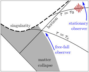
Figure 1: The Kruskal diagram of a Schwarzschild black hole formed from collapse, foliated by hypersurfaces of constant $\tau$. The time at which the horizon emerges is the crossing time denoted by $\tau_{c}$. A Hawking wave packet detected by a stationary observer around $\tau=\tau_{0}$ is traced back in time and decomposed into positive and negative-frequency components with respect to a freely falling observer comoving with the surface of the collapsing matter.

To compute Hawking radiation, we trace the wave packet of a Hawking particle backward in time to the near-horizon region and calculate the norm of its negative-frequency components with respect to a freely falling observer. A generic wave packet for a Hawking particle centered at $\tau=\tau_{0}$ has the form

$$\widetilde{\Psi}_{(\omega_{0},\tau_{0})}(\tau,p)=\int_{0}^{\infty}d\omega\,f_{\omega_{0}}(\omega)\,e^{i\omega\tau_{0}}\,\tilde{\phi}_{\omega}(\tau,p)\,,$$ (3.25)

which is analogous to eq. (2.29), but defined in a different reference frame. At large $\tau$, the wave packet conforms to an ordinary null packet of the low-energy effective theory, and similar to eq. (2.31) in the previous section, its wave function in the position space is approximately a function of $u$ only:

$$\Psi_{\omega_{0}}(u-u_{0})=\frac{1}{\sqrt{2\gamma^{-1/2}\omega_{0}}}\int_{0}^{\infty}d\omega\,f_{\omega_{0}}(\omega)\,e^{-i\gamma^{-1/2}\omega(u-u_{0})}\,,$$ (3.26)

where $u_{0}\equiv\gamma^{1/2}\tau_{0}$.

The wave packet (3.25) is traced back in time to be matched with the free-fall mode expansion (3.24) at around the crossing time $\tau_{c}$ (denoted as $T_{c}$ in the coordinate patch of a freely falling observer) when the collapsing matter is about to pass through the horizon (see figure 1). With $b_{\Psi}$ representing the annihilation operator associated with the Hawking particle described by this wave packet, we obtain from the relativistic inner product (see eq. (2.10))

$$b_{\Psi} =\bigl{\langle}\widetilde{\Psi}_{(\omega_{0},\tau_{0})}(\tau_{c})\bigl{|}\,p\,\bigr{|}\tilde{\phi}(T_{c})\bigr{\rangle}$$

$$=\int_{0}^{\infty}dp\,\sqrt{\frac{p}{2\left(1+\ell^{2}p^{2}\right)}}\left[\widetilde{\Psi}_{(\omega_{0},\tau_{0})}^{*}(\tau_{c}\,,p)\,e^{-i\gamma^{-1/2}\,p\,T_{c}}\,a_{p}-\widetilde{\Psi}_{(\omega_{0},\tau_{0})}^{*}(\tau_{c}\,,-p)\,e^{i\gamma^{-1/2}\,p\,T_{c}}\,a_{p}^{\dagger}\right]\,.$$ (3.27)

Assuming the free-fall vacuum state $\ket{0}$ (Unruh vacuum) annihilated by $a_{p}$ for all positive $p$, we determine the number of Hawking quanta by following the same steps outlined in the previous section, leading to

$$\expectationvalue{b_{\Psi}^{\dagger}b_{\Psi}}{0} =\frac{1}{2}\int_{0}^{\infty}dp\,\frac{p}{1+\ell^{2}p^{2}}\,\absolutevalue\big{\widetilde{\Psi}_{(\omega_{0},\tau_{0})}(\tau_{c},-p)}^{2}$$

$$\approx\frac{a/2}{e^{4\pi a\gamma^{-1/2}\omega_{0}}-1}\int d\omega\,d\omega^{\prime}\,f_{\omega_{0}}^{*}(\omega)\,f_{\omega_{0}}(\omega^{\prime})\,e^{-i(\omega-\omega^{\prime})(\tau_{0}-\tau_{c})}\int_{-\infty}^{\log(a/\ell)}dF\,e^{2ia\gamma^{-1/2}(\omega-\omega^{\prime})F}$$

$$=\frac{1}{2}\,\frac{\gamma^{-1/2}\omega_{0}}{e^{4\pi a\gamma^{-1/2}\omega_{0}}-1}\times\int_{-\infty}^{2a\gamma^{-1/2}\log(a/\ell)-\Delta\tau}d\tau\,\gamma^{1/2}\,\bigl{|}\Psi_{\omega_{0}}(\gamma^{1/2}\tau)\bigr{|}^{2}$$

$$=\frac{1}{2}\,\frac{\gamma^{-1/2}\omega_{0}}{e^{4\pi a\gamma^{-1/2}\omega_{0}}-1}\times\int_{-\infty}^{2a\log(a/\ell)-\Delta t}dt\,\bigl{|}\Psi_{\omega_{0}}(t)\bigr{|}^{2}\,,$$ (3.28)

where $\Delta\tau\equiv\tau_{0}-\tau_{c}$ , $\Delta t\equiv\gamma^{1/2}\Delta\tau$ is the difference in the Schwarzschild time $t$, and $\gamma^{-1/2}\omega_{0}$ is the central frequency of the Hawking particle defined with respect to $t$. As it turns out, the Hawking radiation is turned off when $\Delta\tau\gtrsim 2a\gamma^{-1/2}\log(a/\ell)$. For a distant observer situated at a fixed radius $r$, this shutdown time scale can be expressed as

$$\Delta t\gtrsim 2a\log(a/\ell)\,.$$ (3.29)

This is in agreement with the finding (2.39) presented in the previous section, as $\Delta t$ coincides with $\Delta u$ at a fixed $r$. Strikingly, despite the fact that the implementation of the GUP relies on the choice of coordinates, the final outcome (3.28), from the viewpoint of a stationary observer, is independent of the parameter $\gamma$, which distinguishes different freely falling frames.

4 Conclusion and Discussion

In this work, we studied the effect of the generalized uncertainty principle (GUP) on Hawking radiation in both the Eddington-Finkelstein coordinates and a class of freely falling frames adapted to geodesic observers with different initial velocities at past infinity. Our approach involved deforming the radial coordinate of the black hole background in a way that realizes the minimal length uncertainty relation (1.1). We came to the conclusion that due to the GUP, Hawking radiation is eventually terminated at around the scrambling time $\Delta t\sim 2a\log(a/\ell)$, as measured by a distant observer who is stationary with respect to the black hole. Remarkably, this outcome turns out to be independent of the specific choice of the coordinate system in which the GUP is implemented.

The primary reason that led to the eventual decrease in Hawking radiation at late times is the following. Notice that the effect of the GUP essentially boils down to a substitution of the momentum $p$ with an “effective momentum” $q(p)$ in the evaluation of the number expectation value of Hawking particles (see, for example, eq. (2.36)). This change of variables is encapsulated by the relation

$$p\rightarrow q(p)\equiv\frac{p}{\sqrt{1+\ell^{2}p^{2}}}\,,$$ (4.1)

where the unbounded interval of $p$ is mapped to a finite range of $q$, with a cutoff value given by $q(\infty)=\ell^{-1}$. Consequently, the situation is equivalent to having a UV cutoff $\ell^{-1}$ imposed on the frequency spectrum, which causes a significant reduction in the amplitude of Hawking radiation beyond the scrambling time, a result consistent with the conclusions drawn from earlier works [9, 10].

Nevertheless, we emphasize that the physical interpretation underlying the scenario above with the GUP greatly differs from a mere truncation of the effective field theory via a UV cutoff. In our implementation of the GUP, we did not exclude the presence of trans-Planckian modes. Instead, these modes are simply not expected to play a role in the Hawking process, as elaborated upon in the end of Sec. 2. The reason behind this lies in the fact that the trans-Planckian modes exhibit a large uncertainty $\Delta p\gg a/\ell^{2}$ in momentum, which in turn gives rise to a large uncertainty $\Delta x\gtrsim\ell^{2}p\gg a$ in position implied by the GUP (1.1). Given that the length scales associated with these modes are significantly larger than the size of the black hole, their evolution is more suitably described in the asymptotically flat region far from the black hole, and thus do not lead to particle creation. As a result, the late-time Hawking radiation, which would have originated from trans-Planckian fluctuations in the vacuum near the horizon, would no longer exist once the effects of the GUP are accounted for.

Since Hawking radiation lasts for approximately the scrambling time, only a fraction of the energy of order $\mathcal{O}\bigl{(}(\ell^{2}/a^{2})\log(a/\ell)\bigr{)}$ relative to the original black hole mass will be evaporated away. Therefore, the information loss problem, which typically arises around the Page time $\mathcal{O}(a^{3}/\ell^{2})$ [72], is absent here, and the firewall [73] does not emerge. The emitted radiation is thermal and carries no information. In this sense, incorporating the GUP into the radiation field effectively results in a macroscopic black hole remnant that is essentially classical. This scenario also avoids the issues associated with Planck-size remnants as the end state of evaporation (see, e.g., [74, 75]). Moreover, these findings have significant implications in the context of primordial black holes in the early universe. Considering the substantial distinctions in both the evaporation time scale and the relic masses of primordial black holes under the GUP, we anticipate a completely different number density of black hole remnants produced at the end of inflation. This would impact the proposal that primordial black hole remnants could serve as candidates for dark matter [76, 77, 78].

This study was inspired by a series of investigations that challenged the robustness of Hawking radiation against modifications of UV physics. Notably, it was highlighted in Refs. [7, 8, 9, 10] that non-renormalizable higher-derivative interactions, while featuring coupling constants suppressed by inverse powers of the Planck mass, can induce exponentially large deviations in Hawking radiation that lead to a breakdown of the low-energy effective theory around the scrambling time. Furthermore, a more recent work [27] demonstrated that Hawking radiation could stop at around the scrambling time, at a later time, or persist until the black hole becomes microscopic, depending on the UV behavior of modified dispersion relations. In the present study, we focused on the implications of the GUP, which was originally proposed to capture a certain aspect of string theory. The outcomes of this work confirmed once again that the late-time behavior of the amplitude of Hawking radiation is sensitive to UV physics, although the Hawking temperature remains robust up to perturbative corrections. A more comprehensive check is still required to ascertain whether this is indeed a prediction of string theory. On a broader scope, it is appealing to further explore how the amplitude of Hawking radiation behaves under different candidates of quantum gravity.

Much like other theories incorporating a minimum length, a theory involving the GUP is inherently nonlocal, and thus a large correction to the conventional Hawking radiation is perhaps not very surprising. On the other hand, Hawking radiation in nonlocal theories with a minimum length have been examined before in Refs. [16, 18, 22, 79], which all reported a robust Hawking radiation. The reason why the UV-dependence of Hawking radiation has been missed in the past can be partially attributed to the predominant emphasis on calculating the Hawking temperature, a feature indeed resilient to modifications, while overlooking the magnitude of the radiation, which can undergo substantial changes over time. Another reason is that there are subtleties involved in the notion of a minimum length. Future studies aimed at illuminating the connection between Hawking radiation and UV theories will be valuable.

Appendix A Beyond the Near-Horizon Approximation

In our formulations of GUP-inspired field theory in different coordinate systems of a black hole background, we employed the near-horizon approximation by expanding the spatial dependence around $x=0$ and retaining terms up to $\mathcal{O}(x/a)$ before analyzing the theory in momentum space. In the ingoing Vaidya coordinates (see Sec. 2), this yielded the field equation

$$\left[\partial_{v}+\frac{1}{2}\left(1-\frac{a}{\hat{x}+a}\right)ip\right]\tilde{\phi}(v,p)\approx\left(\partial_{v}+\frac{\hat{x}}{2a}\,ip\right)\tilde{\phi}(v,p)=0\,,$$ (A.1)

whereas in the freely falling coordinates (see Sec. 3), it led to

$$\left[\partial_{\tau}+v_{\gamma}(\hat{x})\,ip+\gamma^{-1/2}ip\right]\tilde{\phi}(\tau,p)\approx\left(\partial_{\tau}+\gamma^{1/2}\,\frac{\hat{x}}{2a}\,ip\right)\tilde{\phi}(\tau,p)=0$$ (A.2)

for the outgoing modes. However, as we implement the representation $\hat{x}=i(1+\ell^{2}p^{2})\partial_{p}$, the $\hat{x}/a$-expansion is no longer a valid approximation at large $\absolutevalue{p}\gg a/\ell^{2}$ due to the factor $(1+\ell^{2}p^{2})$ introduced by GUP corrections. In this appendix, we solve the complete field equation using the exact Vaidya line element (2.4), without relying on the $x/a$-expansion. We find that our conclusion regarding the late-time suppression of Hawking radiation still holds. A similar scenario is expected to apply to the modified field equation (A.2) in the freely falling coordinates.

Let us reframe our analysis in Sec. 2 without restricting to the near-horizon region. Starting with the conventional action (2.6) in the low-energy effective theory now expressed as

$$S_{0}=\frac{1}{2}\int dv\int dr\,\phi(v,r)\,\partial_{r}\,r^{-1}\bigl{\{}2r\,\partial_{v}+\left[r-\Theta(v)\,a\right]\partial_{r}\bigr{\}}\,\phi(v,r)\,,$$ (A.3)

we arrive at the equivalent form in the momentum space as

$$S_{0}=\int dv\int_{-\infty}^{\infty}dp\,\tilde{\phi}^{*}(v,p)\,p\,\hat{r}^{-1}\left\{i\hat{r}\,\partial_{v}-\left[\hat{r}-\Theta(v)\,a\right]\frac{p}{2}\right\}\tilde{\phi}(v,p)\,.$$ (A.4)

We introduce the GUP into the radial coordinate $r$ by adopting the representation

$$\hat{r}\equiv if(p)\,\partial_{p}\,,\qquad\text{where}\quad f(p)=1+\ell^{2}p^{2}\,.$$ (A.5)

In addition, we define the inverse $\hat{r}^{-1}$ as $\hat{r}^{-1}\equiv-i\,\partial_{p}^{-1}f^{-1}(p)$. With the incorporation of the GUP, the momentum-space action (A.4) becomes

$$S_{\text{GUP}}=2\int dv\int_{0}^{\infty}\frac{dp}{f(p)}\,\tilde{\phi}^{*}(v,p)\,p\,\partial_{p}^{-1}f^{-1}(p)\left[f(p)\,\partial_{p}\left(i\partial_{v}-\frac{p}{2}\right)-\Theta(v)\,\frac{ia}{2}\,p\right]\tilde{\phi}(v,p)\,,$$ (A.6)

which leads to the field equation

$$\left[f(p)\,\partial_{p}\left(i\partial_{v}-\frac{p}{2}\right)-\Theta(v)\,\frac{ia}{2}\,p\right]\tilde{\phi}(v,p)=0$$ (A.7)

for the outgoing modes.

Outside the shell ($v>0$), the stationary solutions take on the form

$$\tilde{\phi}_{\omega}(v,p)=\mathcal{N}_{\omega}\,e^{-i\omega v}\,\exp\left[-i\,\frac{a\tan^{-1}(\ell p)}{\ell\left(1+4\ell^{2}\omega^{2}\right)}\right]\times\frac{1}{p-2\omega-i0^{+}}\left[\frac{a\left(p-2\omega-i0^{+}\right)}{\sqrt{1+\ell^{2}p^{2}}}\right]^{-\frac{2ia\omega}{1+4\ell^{2}\omega^{2}}}\,,$$ (A.8)

with the constant $\mathcal{N}_{\omega}$ once again determined by matching a low-frequency ($\omega\ell\ll 1$) wave packet with the standard outgoing wave packet of the low-energy effective theory at large $v\gg u_{0}$, just as in eq. (2.31). For low-energy Hawking particles with $\omega\ll\ell^{-1}$, this yields the same expression for $\mathcal{N}_{\omega}$ as shown in eq. (2.27).

In the flat spacetime inside the shell ($v<0$), the field equation (A.7) reduces to

$$\left(1+\ell^{2}p^{2}\right)\partial_{p}\left(i\partial_{v}-\frac{p}{2}\right)\tilde{\phi}(v<0,p)=0\,,$$ (A.9)

and thus the outgoing sector of the field has the same mode expansion as in eq. (2.17). As a result, the rest of the calculation proceeds in a straightforward manner, resembling the steps taken in Sec. 2. In particular, in place of eq. (2.36), we now have

$$\bigl{\langle}\Theta(p)\,\tilde{\phi}_{\omega}(0,-p)\bigl{|}\,p\,\bigr{|}\Theta(p)\,\tilde{\phi}_{\omega^{\prime}}(0,-p)\bigr{\rangle}$$

$$= \ \mathcal{N}_{\omega}^{*}\,\mathcal{N}_{\omega^{\prime}}\,\exp\left[-2\pi a\left(\frac{\omega}{1+4\ell^{2}\omega^{2}}+\frac{\omega^{\prime}}{1+4\ell^{2}\omega^{\prime\,2}}\right)\right]\int_{0}^{\infty}\frac{dp}{1+\ell^{2}p^{2}}\,\frac{p\,\exp\left[2ia(\omega-\omega^{\prime})F_{\omega\omega^{\prime}}(p)\right]}{(p+2\omega)(p+2\omega^{\prime})}$$

$$= \ \mathcal{N}_{\omega}^{*}\,\mathcal{N}_{\omega^{\prime}}\,\exp\left[-2\pi a\left(\frac{\omega}{1+4\ell^{2}\omega^{2}}+\frac{\omega^{\prime}}{1+4\ell^{2}\omega^{\prime\,2}}\right)\right]\int_{F_{\omega\omega^{\prime}}(0)}^{F_{\omega\omega^{\prime}}(\infty)}dF_{\omega\omega^{\prime}}\,e^{2ia(\omega-\omega^{\prime})F_{\omega\omega^{\prime}}}\,,$$ (A.10)

where

$$F_{\omega\omega^{\prime}}(p)\equiv\frac{1}{\omega-\omega^{\prime}}\,\Biggl{\{} \frac{\omega}{1+4\ell^{2}\omega^{2}}\,\log\left[\frac{a\left(p+2\omega\right)}{\sqrt{1+\ell^{2}p^{2}}}\right]-\frac{\omega^{\prime}}{1+4\ell^{2}\omega^{\prime\,2}}\,\log\left[\frac{a\left(p+2\omega^{\prime}\right)}{\sqrt{1+\ell^{2}p^{2}}}\right]$$ (A.11)

$$+\frac{2\ell\left(\omega^{2}-\omega^{\prime\,2}\right)\tan^{-1}\left(\ell p\right)}{\left(1+4\ell^{2}\omega^{2}\right)\left(1+4\ell^{2}\omega^{\prime\,2}\right)}\Biggr{\}}\,.$$

Similar to the change of variables from $p$ to $F(p)$ in eq. (2.36), the construction of $F_{\omega\omega^{\prime}}(p)$ above serves the purpose of simplifying the $p$-integral in eq. (A.10), taking advantage of the fact that

$$dF_{\omega\omega^{\prime}}=\frac{1}{1+\ell^{2}p^{2}}\,\frac{p}{(p+2\omega)(p+2\omega^{\prime})}\,dp\,.$$ (A.12)

For a large black hole, the typical frequency of Hawking radiation lies in the range $\omega,\omega^{\prime}\sim 1/a\ll\ell^{-1}$, which implies that the upper and lower bounds of the $F_{\omega\omega^{\prime}}$-integration in eq. (A.10) are approximately given by

$$F_{\omega\omega^{\prime}}(\infty)\approx\log(a/\ell)\qquad\text{and}\qquad F_{\omega\omega^{\prime}}(0)\approx\frac{\omega\log(2a\omega)-\omega^{\prime}\log(2a\omega^{\prime})}{\omega-\omega^{\prime}}\sim\mathcal{O}(1)\,,$$ (A.13)

respectively. Subsequently, eq. (2.37) is replaced by

$$\expectationvalue{b_{\Psi}^{\dagger}b_{\Psi}}{0} \approx\frac{a}{2}\,\frac{e^{-4\pi a\omega_{0}}}{1-e^{-4\pi a\omega_{0}}}\int d\omega\,f_{\omega_{0}}^{*}(\omega)\int d\omega^{\prime}\,f_{\omega_{0}}(\omega^{\prime})\,e^{-i(\omega-\omega^{\prime})u_{0}}\int_{F_{\omega\omega^{\prime}}(0)}^{\log(a/\ell)}dF_{\omega\omega^{\prime}}\,e^{2ia(\omega-\omega^{\prime})F_{\omega\omega^{\prime}}}$$

$$=\frac{1}{4}\,\frac{1}{e^{4\pi a\omega_{0}}-1}\int d\omega\,f_{\omega_{0}}^{*}(\omega)\int d\omega^{\prime}\,f_{\omega_{0}}(\omega^{\prime})\int_{2aF_{\omega\omega^{\prime}}(0)-u_{0}}^{2a\log(a/\ell)-u_{0}}du\,e^{i(\omega-\omega^{\prime})u}$$

$$\approx\frac{1}{2}\,\frac{\omega_{0}}{e^{4\pi a\omega_{0}}-1}\times\int_{2a\,\mathcal{O}(1)-u_{0}}^{2a\log(a/\ell)-u_{0}}du\,\bigl{|}\Psi_{\omega_{0}}(u)\bigr{|}^{2}\,.$$ (A.14)

We observe that the Hawking radiation is gradually turned on as $u_{0}$ exceeds $2a\,\mathcal{O}(1)\sim\mathcal{O}(a)$. This transient phenomenon of Hawking radiation becomes evident only when we extend beyond the near-horizon approximation [27]. Most importantly, as the integral in (A.14) is highly suppressed when

$$u_{0}\gtrsim 2a\log(a/\ell)\,,$$ (A.15)

we reach the same conclusion as in Sec. 2 that Hawking radiation is terminated after the scrambling time.

References

- [1] S.W. Hawking, Black hole explosions, Nature 248 (1974) 30.
- [2] S.W. Hawking, Particle Creation by Black Holes, Commun. Math. Phys. 43 (1975) 199.
- [3] S.W. Hawking, Breakdown of Predictability in Gravitational Collapse, Phys. Rev. D 14 (1976) 2460.
- [4] S.D. Mathur, The Information paradox: A Pedagogical introduction, Class. Quant. Grav. 26 (2009) 224001 [arXiv:0909.1038].
- [5] G. ’t Hooft, On the Quantum Structure of a Black Hole, Nucl. Phys. B 256 (1985) 727.
- [6] T. Jacobson, Black hole evaporation and ultrashort distances, Phys. Rev. D 44 (1991) 1731.
- [7] P.M. Ho and Y. Yokokura, Firewall from Effective Field Theory, Universe 7 (2021) 241 [arXiv:2004.04956].
- [8] P.M. Ho, From uneventful Horizon to firewall in D-dimensional effective theory, Int. J. Mod. Phys. A 36 (2021) 2150145 [arXiv:2005.03817].
- [9] P.M. Ho, H. Kawai and Y. Yokokura, Planckian physics comes into play at Planckian distance from horizon, JHEP 01 (2022) 019 [arXiv:2111.01967].
- [10] P.M. Ho and H. Kawai, UV and IR effects on Hawking radiation, JHEP 03 (2023) 002 [arXiv:2207.07122].
- [11] Y. Sekino and L. Susskind, Fast Scramblers, JHEP 10 (2008) 065 [arXiv:0808.2096].
- [12] W.G. Unruh, Sonic analog of black holes and the effects of high frequencies on black hole evaporation, Phys. Rev. D 51 (1995) 2827 [gr-qc/9409008].
- [13] R. Brout, S. Massar, R. Parentani and P. Spindel, Hawking radiation without transPlanckian frequencies, Phys. Rev. D 52 (1995) 4559 [hep-th/9506121].
- [14] N. Hambli and C.P. Burgess, Hawking radiation and ultraviolet regulators, Phys. Rev. D 53 (1996) 5717 [hep-th/9510159].
- [15] S. Corley and T. Jacobson, Hawking spectrum and high frequency dispersion, Phys. Rev. D 54 (1996) 1568 [hep-th/9601073].
- [16] S. Corley and T. Jacobson, Lattice black holes, Phys. Rev. D 57 (1998) 6269 [hep-th/9709166].
- [17] S. Corley, Computing the spectrum of black hole radiation in the presence of high frequency dispersion: An Analytical approach, Phys. Rev. D 57 (1998) 6280 [hep-th/9710075].
- [18] T. Jacobson and D. Mattingly, Hawking radiation on a falling lattice, Phys. Rev. D 61 (2000) 024017 [hep-th/9908099].
- [19] W.G. Unruh and R. Schützhold, On the universality of the Hawking effect, Phys. Rev. D 71 (2005) 024028 [gr-qc/0408009].
- [20] C. Barcelo, S. Liberati and M. Visser, Analogue gravity, Living Rev. Rel. 8 (2005) 12 [gr-qc/0505065].
- [21] I. Agullo, J. Navarro-Salas, G.J. Olmo and L. Parker, Insensitivity of Hawking radiation to an invariant Planck-scale cutoff, Phys. Rev. D 80 (2009) 047503 [arXiv:0906.5315].
- [22] N. Kajuri and D. Kothawala, Universality of Hawking radiation in non local field theories, Phys. Lett. B 791 (2019) 319 [arXiv:1806.10345].
- [23] T. Jacobson, Black hole radiation in the presence of a short distance cutoff, Phys. Rev. D 48 (1993) 728 [hep-th/9303103].
- [24] A.D. Helfer, Do black holes radiate?, Rept. Prog. Phys. 66 (2003) 943 [gr-qc/0304042].
- [25] C. Barcelo, L.J. Garay and G. Jannes, Sensitivity of Hawking radiation to superluminal dispersion relations, Phys. Rev. D 79 (2009) 024016 [arXiv:0807.4147].
- [26] E.T. Akhmedov, H. Godazgar and F.K. Popov, Hawking radiation and secularly growing loop corrections, Phys. Rev. D 93 (2016) 024029 [arXiv:1508.07500].
- [27] E.T. Akhmedov, T.L. Chau, P.M. Ho, H. Kawai, W.H. Shao and C.T. Wang, UV Dispersive Effects on Hawking Radiation, arXiv:2307.12831.
- [28] L.J. Garay, Quantum gravity and minimum length, Int. J. Mod. Phys. A 10 (1995) 145 [gr-qc/9403008].
- [29] A.F. Ali, S. Das and E.C. Vagenas, Discreteness of Space from the Generalized Uncertainty Principle, Phys. Lett. B 678 (2009) 497 [arXiv:0906.5396].
- [30] D. Amati, M. Ciafaloni and G. Veneziano, Superstring Collisions at Planckian Energies, Phys. Lett. B 197 (1987) 81.
- [31] D.J. Gross and P.F. Mende, The High-Energy Behavior of String Scattering Amplitudes, Phys. Lett. B 197 (1987) 129.
- [32] D.J. Gross and P.F. Mende, String Theory Beyond the Planck Scale, Nucl. Phys. B 303 (1988) 407.
- [33] D. Amati, M. Ciafaloni and G. Veneziano, Can Space-Time Be Probed Below the String Size?, Phys. Lett. B 216 (1989) 41.
- [34] M. Fabbrichesi and G. Veneziano, Thinning Out of Relevant Degrees of Freedom in Scattering of Strings, Phys. Lett. B 233 (1989) 135.
- [35] K. Konishi, G. Paffuti and P. Provero, Minimum Physical Length and the Generalized Uncertainty Principle in String Theory, Phys. Lett. B 234 (1990) 276.
- [36] R. Guida, K. Konishi and P. Provero, On the short distance behavior of string theories, Mod. Phys. Lett. A 6 (1991) 1487.
- [37] M. Maggiore, A Generalized uncertainty principle in quantum gravity, Phys. Lett. B 304 (1993) 65 [hep-th/9301067].
- [38] F. Scardigli, Generalized uncertainty principle in quantum gravity from micro - black hole Gedanken experiment, Phys. Lett. B 452 (1999) 39 [hep-th/9904025].
- [39] R.J. Adler and D.I. Santiago, On gravity and the uncertainty principle, Mod. Phys. Lett. A 14 (1999) 1371 [gr-qc/9904026].
- [40] S. Capozziello, G. Lambiase and G. Scarpetta, Generalized uncertainty principle from quantum geometry, Int. J. Theor. Phys. 39 (2000) 15 [gr-qc/9910017].
- [41] F. Scardigli and R. Casadio, Generalized uncertainty principle, extra dimensions and holography, Class. Quant. Grav. 20 (2003) 3915 [hep-th/0307174].
- [42] A. Kempf, G. Mangano and R.B. Mann, Hilbert space representation of the minimal length uncertainty relation, Phys. Rev. D 52 (1995) 1108 [hep-th/9412167].
- [43] A. Kempf, On quantum field theory with nonzero minimal uncertainties in positions and momenta, J. Math. Phys. 38 (1997) 1347 [hep-th/9602085].
- [44] A. Kempf and G. Mangano, Minimal length uncertainty relation and ultraviolet regularization, Phys. Rev. D 55 (1997) 7909 [hep-th/9612084].
- [45] S. Detournay, C. Gabriel and P. Spindel, About maximally localized states in quantum mechanics, Phys. Rev. D 66 (2002) 125004 [hep-th/0210128].
- [46] S. Segreto and G. Montani, Extended GUP formulation and the role of momentum cut-off, Eur. Phys. J. C 83 (2023) 385 [arXiv:2208.03101].
- [47] R. Brout, C. Gabriel, M. Lubo and P. Spindel, Minimal length uncertainty principle and the transPlanckian problem of black hole physics, Phys. Rev. D 59 (1999) 044005 [hep-th/9807063].
- [48] F. Scardigli, M. Blasone, G. Luciano and R. Casadio, Modified Unruh effect from Generalized Uncertainty Principle, Eur. Phys. J. C 78 (2018) 728 [arXiv:1804.05282].
- [49] G. Amelino-Camelia, M. Arzano, Y. Ling and G. Mandanici, Black-hole thermodynamics with modified dispersion relations and generalized uncertainty principles, Class. Quant. Grav. 23 (2006) 2585 [gr-qc/0506110].
- [50] K. Nozari and S. Hamid Mehdipour, Quantum Gravity and Recovery of Information in Black Hole Evaporation, EPL 84 (2008) 20008 [arXiv:0804.4221].
- [51] B. Majumder, Black Hole Entropy with minimal length in Tunneling formalism, Gen. Rel. Grav. 45 (2013) 2403 [arXiv:1212.6591].
- [52] D.Y. Chen, Q.Q. Jiang, P. Wang and H. Yang, Remnants, fermions‘ tunnelling and effects of quantum gravity, JHEP 11 (2013) 176 [arXiv:1312.3781].
- [53] Y.G. Miao, Y.J. Zhao and S.J. Zhang, Maximally localized states and quantum corrections of black hole thermodynamics in the framework of a new generalized uncertainty principle, Adv. High Energy Phys. 2015 (2015) 627264 [arXiv:1410.4115].
- [54] P. Wang, H. Yang and S. Ying, Quantum gravity corrections to the tunneling radiation of scalar particles, Int. J. Theor. Phys. 55 (2016) 2633 [arXiv:1410.5065].
- [55] D. Chen, H. Wu, H. Yang and S. Yang, Effects of quantum gravity on black holes, Int. J. Mod. Phys. A 29 (2014) 1430054 [arXiv:1410.5071].
- [56] P. Bargueño and E.C. Vagenas, Semiclassical corrections to black hole entropy and the generalized uncertainty principle, Phys. Lett. B 742 (2015) 15 [arXiv:1501.03256].
- [57] B. Mu, P. Wang and H. Yang, Minimal Length Effects on Tunnelling from Spherically Symmetric Black Holes, Adv. High Energy Phys. 2015 (2015) 898916 [arXiv:1501.06025].
- [58] I. Sakalli, A. Övgün and K. Jusufi, GUP Assisted Hawking Radiation of Rotating Acoustic Black Holes, Astrophys. Space Sci. 361 (2016) 330 [arXiv:1602.04304].
- [59] G. Gecim and Y. Sucu, The GUP effect on Hawking radiation of the 2 + 1 dimensional black hole, Phys. Lett. B 773 (2017) 391 [arXiv:1704.03536].
- [60] G. Lambiase and F. Scardigli, Lorentz violation and generalized uncertainty principle, Phys. Rev. D 97 (2018) 075003 [arXiv:1709.00637].
- [61] T. Kanazawa, G. Lambiase, G. Vilasi and A. Yoshioka, Noncommutative Schwarzschild geometry and generalized uncertainty principle, Eur. Phys. J. C 79 (2019) 95.
- [62] L. Buoninfante, G.G. Luciano and L. Petruzziello, Generalized Uncertainty Principle and Corpuscular Gravity, Eur. Phys. J. C 79 (2019) 663 [arXiv:1903.01382].
- [63] T. Ibungochouba Singh, Y.K. Meitei and I.A. Meitei, Effect of GUP on Hawking radiation of BTZ black hole, Int. J. Mod. Phys. A 35 (2020) 2050018 [arXiv:1910.09288].
- [64] S. Kanzi and I. Sakallı, GUP-modified Hawking radiation and transmission/reflection coefficients of rotating polytropic black hole, Eur. Phys. J. Plus 137 (2022) 14 [arXiv:2107.11776].
- [65] M.A. Anacleto, F.A. Brito, G.C. Luna and E. Passos, The generalized uncertainty principle effect in acoustic black holes, Annals Phys. 440 (2022) 168837 [arXiv:2112.13573].
- [66] M.A. Anacleto, F.A. Brito and E. Passos, Hawking radiation and stability of the canonical acoustic black holes, Annals Phys. 455 (2023) 169364 [arXiv:2212.13850].
- [67] M.A. Anacleto, F.A. Brito, E. Passos, J.L. Paulino, A.T.N. Silva and J. Spinelly, Hawking radiation and entropy of a BTZ black hole with minimum length, Mod. Phys. Lett. A 37 (2022) 2250215 [arXiv:2301.05970].
- [68] Y.C. Ong, A critique on some aspects of GUP effective metric, Eur. Phys. J. C 83 (2023) 209 [arXiv:2303.10719].
- [69] M.A. Anacleto, F.A. Brito and E. Passos, Modified metrics of acoustic black holes: A review, Biophys. J. 7 (2023) 000245 [arXiv:2306.03077].
- [70] E. Ievlev and M.R.R. Good, Thermal Larmor radiation, arXiv:2303.03676.
- [71] T. Damour and R. Ruffini, Black Hole Evaporation in the Klein-Sauter-Heisenberg-Euler Formalism, Phys. Rev. D 14 (1976) 332.
- [72] D.N. Page, Information in black hole radiation, Phys. Rev. Lett. 71 (1993) 3743 [hep-th/9306083].
- [73] A. Almheiri, D. Marolf, J. Polchinski and J. Sully, Black Holes: Complementarity or Firewalls?, JHEP 02 (2013) 062 [arXiv:1207.3123].
- [74] P. Chen, Y.C. Ong and D.h. Yeom, Black Hole Remnants and the Information Loss Paradox, Phys. Rept. 603 (2015) 1 [arXiv:1412.8366].
- [75] Y.C. Ong, Generalized Uncertainty Principle, Black Holes, and White Dwarfs: A Tale of Two Infinities, JCAP 09 (2018) 015 [arXiv:1804.05176].
- [76] J.H. MacGibbon, Can Planck-mass relics of evaporating black holes close the universe?, Nature 329 (1987) 308.
- [77] P. Chen and R.J. Adler, Black hole remnants and dark matter, Nucl. Phys. B Proc. Suppl. 124 (2003) 103 [gr-qc/0205106].
- [78] D. Baumann, P.J. Steinhardt and N. Turok, Primordial Black Hole Baryogenesis, hep-th/0703250.
- [79] J. Boos, V.P. Frolov and A. Zelnikov, Ghost-free modification of the Polyakov action and Hawking radiation, Phys. Rev. D 100 (2019) 104008 [arXiv:1909.01494].
- [80] Y.C. Ong and M.R.R. Good, Quantum atmosphere of Reissner-Nordström black holes, Phys. Rev. Res. 2 (2020) 033322 [arXiv:2003.10429].