A Divide and Conquer Approximation Algorithm for Partitioning Rectangles

Abstract

Given a rectangle $R$ with area $A$ and a set of areas $L=\{A_{1},...,A_{n}\}$ with $\sum_{i=1}^{n}A_{i}=A$, we consider the problem of partitioning $R$ into $n$ sub-regions $R_{1},...,R_{n}$ with areas $A_{1},...,A_{n}$ in a way that the total perimeter of all sub-regions is minimized. The goal is to create square-like sub-regions, which are often more desired. We propose an efficient $1.203$–approximation algorithm for this problem based on a divide and conquer scheme that runs in $\mathcal{O}(n^{2})$ time. For the special case when the aspect ratios of all rectangles are bounded from above by 3, the approximation factor is $2/\sqrt{3}\leq 1.1548$. We also present a modified version of out algorithm as a heuristic that achieves better average and best run times.

1 Introduction

Partitioning of a rectangle into several sub-rectangles while optimizing some partition metric is a well-known geometric optimization problem with many different applications such as plant layout design [1, 2, 3, 4, 5], geographic resource allocation [6, 7, 8, 9, 10, 11], treemapping in data visualization [12, 13, 14, 15, 16, 17, 18], VLSI Design [19, 20, 21, 22, 23], and data assignment problem in parallel computers [24, 25, 26, 27].

This problem is also closely-related to many geometric and space partitioning optimization problems that include packing, covering, and tiling—generally focused on minimizing wasted space or optimally allocating geographical resources, as well as data visualization problems–focusing on finding solutions that are visually appealing. These problems include: cutting stock; knapsack; bin packing; guillotine; disk covering; polygon covering; kissing number; strip packing; rectangle packing; square packing; squaring the square; squaring the plane; and, in 3D space, cubing the cube; tetrahedron packing; and treemapping. Our problem is also called soft rectangle packing in the terminology of packing problems. These problems have a large body of literature and a long history that can be perhaps traced back to some geometric problems in the ancient era such as Queen Dido’s problem in ancient Carthage [28].

In this paper, we consider the following problem. Given a rectangle $R$ with $\mathop{\rm Area}\nolimits(R)=A$ and a list of areas $A_{1},...,A_{n}$ with $\sum_{i=1}^{n}A_{i}=A$ we want to partition $R$ into $n$ sub-rectangles with areas $A_{1},...,A_{n}$ in a way that resulting rectangles are as square as possible. It is a common desire in various fields to have square-like rectangles. For this goal we try to minimize the sum of the perimeters of all sub-rectangles. Our choice of the total (average) perimeter is motivated by the fact that the perimeter of a rectangle is minimized when it is a square. We define the perimeter of $R$ as $\mathop{\rm Perim}(R)=\mathop{\rm width}(R)+\mathop{\rm height}(R)$. We also define the aspect ratio of a rectangle $R$ as

$$\mathop{\rm AR}(R)=\max\left\{\frac{\mathop{\rm width}(R)}{\mathop{\rm height}(R)},\frac{\mathop{\rm height}(R)}{\mathop{\rm width}(R)}\right\},$$

i.e., $\mathop{\rm AR}\geq 1$ and the aspect ratio of a square is one.

The NP-hardness of the problem with different objective functions has been proved in several ways. In data visualization field this problem with the goal of minimizing the maximum aspect ratio of all sub-rectangles—was noted as NP-hard by Bruls et al. [15]. de Berg et al. later proved the problem is strongly NP-hard with a reduction from the square packing problem [29]. The related problem of minimizing the total perimeter of all sub-rectangles was proved by Beaumont et al. [25] to be NP-hard, using a reduction from the problem of partitioning a set of integers into two subsets of equal sum. Given this computational complexity, we settle with non-exact approaches and develop one approximation algorithm and one heuristic algorithm to find high quality partitions efficiently.

2 Algorithm

In this section, we propose an approximation algorithm based on a divide and conquer scheme. Divide & conquer approach has been previously used for this problem as in [30, 31, 32, 33], where the approximation guarantee is provided in the first two works. The divide & conquer approach presented by Nagamochi and Abe in [30], suggests a factor 1.25 approximation algorithm. Fügenschuh et al. [31] modified this algorithm and achieved better result for some instances and worse on some others. In their analysis, they distinguish slow-decreasing and fast-decreasing sequences of areas. Slow-decreasing sequences refer to the case where the areas are of similar size. For such sequence of areas the approximation ratio of their algorithm is $2/\sqrt{3}\leq 1.1548$. For the faster-decreasing sequences they find an upper bound for the approximation ratio that depends on the decaying rate and is bounded above by 1.7657. Our algorithm improves these results, which to the best of our knowledge are still the best among the existing algorithms.

1

Input: Rectangle $R$ and a list of $n$ areas $L=\{A_{1},A_{2},...,A_{n}\}$ with $\sum_{i=1}^{n}A_{i}=\mathop{\rm Area}\nolimits(R)$.

Output: Partition $R_{1},R_{2},...,R_{n}$ with areas $A_{1},A_{2},...,A_{n}$.

/* *********************************************** */

2 Function main(R,L)

3        if $n=1$ then

4               return $R$;

5       else

6               Let $w=\mathop{\rm width}(R)$ and $h=\mathop{\rm height}(R)$;

7               Sort $L$ in a non-increasing order and reindex the sorted areas as $A_{1},A_{2},...,A_{n}$;

8               return ${\sf Partition}(R,L,1,n)$;

9              

10        end if

11       

12

1 Procedure Partition($Q,\Lambda,\mbox{start, stop}$)

2        Let $B_{(\cdot)}=\{A_{i},...,A_{j}\}$ denote a block of areas with $\mathop{\rm Area}\nolimits(B_{(\cdot)})=\sum_{k=i}^{j}A_{k}$;

3        Set $L^{\prime}=\{B_{(1)},...,B_{(n)}\}$, where $B_{(i)}=\{A_{i}\},\;\forall i$;

4        Set $L^{\prime\prime}=\{a_{1},a_{2},...,a_{n}\}$, where $a_{i}=\mathop{\rm Area}\nolimits(B_{(i)}),\;\forall i$;

5        while $\left|L^{\prime\prime}\right|>2$ do

6               Set $m=\left|L^{\prime\prime}\right|-1$;

7               Set $a_{m}=a_{m}+a_{m+1}$;

8               Insert $a_{m}$ back into $L^{\prime\prime}$ at location $k$ with $1\leq k\leq m$ that keeps $L^{\prime\prime}$ sorted;

9               Set $B_{(m)}=\cup_{j=m}^{\left|L^{\prime\prime}\right|}B_{(j)}$ and $L^{\prime}=\{B_{(1)},...,B_{(k-1)},B_{(m)},B_{(k)},...,B_{(m-1)}\}$;

10               if $k\neq m$ then

11                      Reindex the blocks in $L^{\prime}$ as $B_{(1)},B_{(2)},...,B_{(m)}$;

12                      Reindex the areas in $L^{\prime\prime}$ as $a_{1},a_{2},...,a_{m}$;

13                     

14               end if

15              

16        end while

17       Set $\Lambda_{1}=L^{\prime}(1)=B_{(1)}$ and $\Lambda_{2}=L^{\prime}(2)=B_{(2)}$;

18        Let $w$ denote the width of $Q$ and $h$ be the height;

19        if $w>h$ then

20               Divide $Q$ with a vertical line into two pieces $Q_{1}$ and $Q_{2}$ with area $L^{\prime\prime}(1)=a_{1}$ on the left and $L^{\prime\prime}(2)=a_{2}$ on the right;

21       else

22               Divide $Q$ with a horizontal line into two pieces $Q_{1}$ and $Q_{2}$ with area $L^{\prime\prime}(1)=a_{1}$ on the top and $L^{\prime\prime}(2)=a_{2}$ on the bottom;

23        end if

24       return $\textnormal{{Partition}}(Q_{1},\Lambda_{1})\cup\textnormal{{Partition}}(Q_{2},\Lambda_{2})$;

25       

26

Algorithm 1 Algorithm ${\sf ApproximationDC}(R,L)$; it takes as input a rectangle and a list of areas. It generates a treemap of sub-rectangles with the given areas according to a divide and conquer approach.

In our Approximate D&C algorithm, we first sort the areas in a non-ascending order and then recursively merge the two smallest areas, while retaining the list of areas sorted, to finally end up with two compounded areas. Then, we partition $R$ into two segments, horizontally or vertically, with these two compounded areas and apply the algorithm to each of these segments. The pseudocode for Approximate D&C, for the case where cuts are either vertical or horizontal (depending on the width & height of the remaining segment), is shown in algorithm 1. It should be noted that it can be generalized to polygonal and angular cuts and has no restriction on input layout container shape. However, our approximation factor analysis here is restricted to the case where the input shape is a rectangle and the cuts are rectangular. This algorithm achieves computational time of $\mathcal{O}(n^{2})$.

1

Input: Rectangle $R$ and a list of $n$ areas $L=\{A_{1},A_{2},...,A_{n}\}$ with $\sum_{i=1}^{n}A_{i}=\mathop{\rm Area}\nolimits(R)$.

Output: Partition $R_{1},R_{2},...,R_{n}$ with areas $A_{1},A_{2},...,A_{n}$.

/* *********************************************** */

2 Function main(R,L)

3        if $n=1$ then

4               return $R$;

5       else

6               Let $w=\mathop{\rm width}(R)$ and $h=\mathop{\rm height}(R)$;

7               Sort $L$ in a non-increasing order and reindex the sorted areas as $A_{1},A_{2},...,A_{n}$;

8               return ${\sf Partition}(R,L,1,n)$;

9              

10        end if

11       

12

1 Procedure Partition($Q,\Lambda,\mbox{start, stop}$)

2        Let $B_{(\cdot)}=\{A_{i},...,A_{j}\}$ denote a block of areas with $\mathop{\rm Area}\nolimits(B_{(\cdot)})=\sum_{k=i}^{j}A_{k}$;

3        Set $L^{\prime}=\{B_{(1)},...,B_{(n)}\}$, where $B_{(i)}=\{A_{i}\},\;\forall i$;

4        Set $L^{\prime\prime}=\{a_{1},a_{2},...,a_{n}\}$, where $a_{i}=\mathop{\rm Area}\nolimits(B_{(i)}),\;\forall i$;

5        while $\left|L^{\prime\prime}\right|>2$ do

6               Set threshold $\tau=\sum_{i=1}^{\left|L^{\prime\prime}\right|}a_{i}\,/\left|L^{\prime\prime}\right|$;

7               Find the smallest $i$ such that $a_{i}<\tau$;

8               if  $i<\left|L^{\prime\prime}\right|$ then

9                     $m=i$;

10                     

11              else

12                      Set $m=\lceil\left|L^{\prime\prime}\right|/2\rceil$;

13                     

14               end if

15              Set $a_{m}=\sum_{j=m}^{\left|L^{\prime\prime}\right|}a_{j}$ and $L^{\prime\prime}=\{a_{1},...,a_{m-1}\}$;

16               Insert $a_{m}$ back into $L^{\prime\prime}$ at location $k$ with $1\leq k\leq m$ that keeps $L^{\prime\prime}$ sorted;

17               Set $B_{(m)}=\cup_{j=m}^{\left|L^{\prime\prime}\right|}B_{(j)}$ and $L^{\prime}=\{B_{(1)},...,B_{(k-1)},B_{(m)},B_{(k)},...,B_{(m-1)}\}$;

18               if $k\mathrel{\mathtt{!=}}m$ then

19                      Reindex the areas in $L^{\prime\prime}$ as $a_{1},a_{2},...,a_{m}$;

20                      Reindex the blocks in $L^{\prime}$ as $B_{(1)},B_{(2)},...,B_{(m)}$;

21                     

22               end if

23              

24        end while

25       Set $\Lambda_{1}=L^{\prime}(1)=B_{(1)}$ and $\Lambda_{2}=L^{\prime}(2)=B_{(2)}$;

26        Let $w$ denote the width of $Q$ and $h$ be the height;

27        if $w>h$ then

28               Divide $Q$ with a vertical line into two pieces $Q_{1}$ and $Q_{2}$ with area $L^{\prime\prime}(1)$ on the left and $L^{\prime\prime}(2)$ on the right;

29              

30       else

31               Divide $Q$ with a horizontal line into two pieces $Q_{1}$ and $Q_{2}$ with area $L^{\prime\prime}(1)$ on the top and $L^{\prime\prime}(2)$ on the bottom;

32              

33        end if

34       return $\textnormal{{Partition}}(Q_{1},\Lambda_{1})\cup\textnormal{{Partition}}(Q_{2},\Lambda_{2})$;

35       

36

Algorithm 2 Modified D&C $(R,L)$ Generates a rectangular treemap with the given areas and bounding rectangle according to a divide and conquer approach.

2.1 Improving the Best and Average Running Times

Bundling the two smallest areas, could be modified to reduce $\mathcal{O}(n)$ such operations in the list. This may change the quality of the solution, since we would no longer have the approximation guarantee. However, having a faster alternative of the algorithm could often be useful. In our Modified D&C algorithm we first sort the areas in a non-ascending order and then recursively merge all areas below some threshold to finally end up with two compounded areas. Here, we set the threshold to be the average of considered areas in each iteration. If at any point we have more than two areas and none of them is below the threshold, we divide the list by half and then sum them to finally end up with two total subareas. Then, similar to algorithm 1, we partition $R$ into two segments with these two compounded areas and apply the algorithm to each of these two segments. The worst case of these two algorithms is the same but the best and average performance in algorithm 2 improves. The magnitude of this improvement highly depends on the input list that determines the behavior aroud the set threshold $\tau$ in each iteration and the number of times the input list gets divided by 2 in each recursive call.

The pseudocode for Modified D&C, for the case where cuts are either vertical or horizontal (depending on the width & height of the remaining segment), is shown in algorithm 2. As shown in the divide & conquer of [32], it can be easily modified and generalized to handle polygonal and angular cuts and to have no restriction on input layout container shape. This is also true for Approximate D&C but in this paper we only analyze the approximation guarantee for the case when we have rectangular input region and output sub-regions.

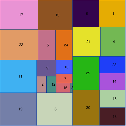
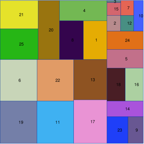
Figure 1: Illustration of the output on a random instance with 25 areas by algorithm 1 at the top with total perimeter of 19.0773 and algorithm 2 on the bottom with total perimeter of 19.5197. Sub-rectangle follow the same labeling and color coding.

2.2 Analysis of Approximate Divide and Conquer

Our approach in the analysis of Approximate D&C is in the same spirit of [30], although our algorithm is totally different. We begin with some definitions we use in proving some critical characteristics of our algorithm and then we introduce the lower and upper bounds.

2.2.1 Critical Characteristics

Let $\mathcal{R}=\{R_{1},...,R_{n}\}$ be a partition of $R$ output by algorithm 1. Rectangles $R_{i}$ in this output are called simple rectangles. Any intermediary input for some recursive call of algorithm 1 is called a compound rectangle. Every call of the algorithm dissects an input region $R$ into two rectangles $R_{1}$ and $R_{2}$. For simplicity, we call them the left child and the right child, respectively, regardless of their actual positioning.

Lemma 1.

Algorithm 1 recursively partitions a rectangle $R$ containing rectangles $R^{\prime}_{i},R^{\prime}_{i+1},...,R^{\prime}_{k}$ with areas $A_{i}\geq A_{i+1}\geq\cdots\geq A_{k}$ into two rectangles $R_{1}$ and $R_{2}$ such that $\mathop{\rm Area}\nolimits(R_{1})\geq\frac{1}{3}\mathop{\rm Area}\nolimits(R)$ and if $A_{i}\leq\frac{2}{3}\mathop{\rm Area}\nolimits(R)$, then we also have $\mathop{\rm Area}\nolimits(R_{2})\geq\frac{1}{3}\mathop{\rm Area}\nolimits(R)$.

Proof.

If $A_{i}\geq\frac{1}{2}\mathop{\rm Area}\nolimits(R)$, its order in the list never changes and the other sub-areas get summed up until only two areas remain in the list, where $\mathop{\rm Area}\nolimits(R_{1})=A_{i}$ will be the first one. As a result, in this case, if $\frac{1}{2}\mathop{\rm Area}\nolimits(R)\leq\mathop{\rm Area}\nolimits(R_{1})\leq\frac{2}{3}\mathop{\rm Area}\nolimits(R)$, we will have $\mathop{\rm Area}\nolimits(R_{2})\geq\frac{1}{3}\mathop{\rm Area}\nolimits(R)$, otherwise, $\mathop{\rm Area}\nolimits(R_{2})\leq\frac{1}{3}\mathop{\rm Area}\nolimits(R)$.
Next we consider the case $\frac{1}{2}\mathop{\rm Area}\nolimits(R)>A_{i}\geq A_{i+1}\geq\cdots\geq A_{k}$. Right before we end up with the final two children $R_{1}$ and $R_{2}$, we have three sub-areas. Let them be $a_{1},a_{2}$ and $a_{3}$. If $a_{1}=A_{i}\leq\frac{1}{2}\mathop{\rm Area}\nolimits(R)$, it should be also greater than $\frac{1}{3}\mathop{\rm Area}\nolimits(R)$, otherwise it could not be located at the beginning of the list. If $a_{1}$ is not the area of an original rectangle of the input list, it should be summation of two other sub-areas that have areas less than $a_{2}$ and $a_{3}$. So, we have $a_{1}\geq a_{2}\geq a_{3}$ and $a_{1}\leq a_{2}+a_{3}\leq 2a_{1}$. Hence, $\mathop{\rm Area}\nolimits(R_{1})=a_{2}+a_{3}$ and $\mathop{\rm Area}\nolimits(R_{2})=a_{1}$. As a result, we have $\nicefrac{{a_{1}}}{{(a_{1}+a_{2}+a_{3})}}\geq\nicefrac{{1}}{{3}}$ and thus $\mathop{\rm Area}\nolimits(R_{1})\geq a_{1}\geq\frac{1}{3}\mathop{\rm Area}\nolimits(R)$. ∎

Lemma 2.

Let $R_{1}$ and $R_{2}$ be the left and right children of a compound rectangle R, and let $A_{\ell}\geq A_{\ell+1}\geq...\geq A_{m}$ be the sub-areas of $A(R)$. Then,

1. $\mathop{\rm AR}(R_{1})\leq\max\{\mathop{\rm AR}(R),3\}$ ,

2. $\mathop{\rm AR}(R_{2})\leq\max\{\mathop{\rm AR}(R),3,(1+\frac{A_{\ell}}{A_{\ell+1}})\}$.

Moreover, if $\mathop{\rm AR}(R_{2})>3$ and $\mathop{\rm AR}(R)\leq\mathop{\rm AR}(R_{2})$, then $R_{1}$ is a simple rectangle with $\mathop{\rm Area}\nolimits(R_{1})=A_{\ell}>\frac{2}{3}\mathop{\rm Area}\nolimits(R)$ and $\mathop{\rm AR}(R_{2})\leq 1+\frac{A_{\ell}}{A_{\ell+1}}$.

Proof.

The proof is the same as the proof of Lemma 3.1 in [30]. ∎

Corollary 3.

Given a rectangle $R$ and a list $L=\{A_{\ell},A_{\ell},...,A_{m}\}$ with $\sum_{A_{i}\in L}A_{i}=\mathop{\rm Area}\nolimits(R)$ and $A_{\ell}\geq A_{\ell+1}\geq...\geq A_{m}$, let $\mathcal{R}=\{R_{\ell},R_{\ell+1},...,R_{m}\}$ be the output of Algorithm ${\sf ApproximationDC}(R,L)$. Let $\mathcal{R^{\prime}}$ be the set of all rectangles that are the input of some recursive call of ${\sf ApproximationDC}(R,L)$. Then, for each rectangle $\hat{R}\in\mathcal{R}\cup\mathcal{R^{\prime}}$ we have

$$\mathop{\rm AR}(\hat{R})\leq\max\{\mathop{\rm AR}(R),3,(1+\max_{A_{i}\in L}\frac{A_{i}}{A_{i+1}})\}$$ (1)

Proof.

By Lemma 2 we have $\max\{\mathop{\rm AR}(R_{1}),\mathop{\rm AR}(R_{2})\}\leq\max\{\mathop{\rm AR}(R),3,(1+\frac{A_{\ell}}{A_{\ell+1}})\}$ for $A_{\ell}=\max_{A_{i}\in L}A_{i}$. Then, (1) follows by induction. ∎

2.2.2 Lower Bound

In order to find lower bounds, we first adopt the definition of forced rectangles from [30].

Definition 4.

The original rectangle $R$ is a forced rectangle. The right child $R_{2}$ of $R$ is a forced rectangle if $A_{1}\geq\mathop{\rm Area}\nolimits(R)/2$. Any rectangle whose long edges are both contained in the long edges of a forced rectangle is defined to be a forced rectangle.

Note that the parent of any forced rectangle is also a forced rectangle.

Lemma 5.

Given a rectangle $R$ and a list $L=\{A_{1},A_{2},...,A_{n}\}$ with $\sum_{A_{i}\in L}A_{i}=\mathop{\rm Area}\nolimits(R)$, let $\mathcal{R}=\{R_{1},...,R_{n}\}$ be a partition of $R$. For any $R_{i}\in\mathcal{R}$ let $\mathop{\rm LB}_{i}$ denote a lower bound on $\mathop{\rm Perim}(R_{i})$. Then,

1. for any forced simple rectangle $R_{i}\in\mathcal{R}$, $\mathop{\rm LB}_{i}=\mathop{\rm width}(R_{i})+\mathop{\rm height}(R_{i})$ is the tight lower bound on $\mathop{\rm Perim}(R_{i})$.

2. for any non-forced simple rectangles $R_{j}\in\mathcal{R}$, we have $\mathop{\rm Perim}(R_{j})\geq\mathop{\rm LB}_{j}=2\sqrt{A_{j}}$.

Proof.

The lower bound in (i) follows from the fact that the length of a short edge of $R_{i}$ cannot be larger than $\min\{\mathop{\rm height}(R_{i}),\mathop{\rm width}(R_{i})\}$ in any other partitioning scheme of $R$. The lower bound in (ii) is trivial. ∎

2.2.3 Upper Bound

The upper bound in our algorithm highly depends on the aspect ratio of the generated sub-rectangles in the partition. Therefore, we break the analysis into different cases depending on aspect ratios.

Case I $(\bm{\mathop{\rm AR}(R_{i})\leq 3,\;i=1,...,n)}$: If all sub-rectangles created by our algorithm either have aspect ratios less than 3 or are simple forced rectangles we will have the approximation factor less than $2/\sqrt{3}<1.1548$. This can be simply shown by the fact that for simple forced rectangles the ratio is 1 and for the other case we have

where the first inequality comes from the fact that all summands in both numerator and denominator are positive reals.

Case II $(\bm{\mathop{\rm AR}(R_{i})>3,\;\textrm{ for some }i)}$: Suppose at some point in our algorithm we come up with a rectangle with aspect ratio greater than 3. We will find the worst case scenarios in terms of approximation factor. For simplicity of notation in the analysis, here we use $\rho$ to denote the aspect ratio.

Lemma 6.

If the algorithm divides $R$ into two rectangles $R_{1}$ and $R_{2}$ and $\mathop{\rm Area}\nolimits(R_{2})=z,\;\mathop{\rm width}(R_{2})=w_{z},\;\mathop{\rm height}(R_{2})=h_{z}$ (with $w_{z}\geq h_{z}$), and $\mathop{\rm AR}(R_{2})=\rho_{z}\geq 3$, which makes the total approximation factor to come above $2/\sqrt{3}$, the approximation factor will be maximized when $R_{2}$ is further divided into $R_{z1}$ and $R_{z2}$, where $R_{z1}$ is a simple rectangle and $R_{z2}$ has $w_{R_{z2}}\leq h_{R_{z2}}$.

Proof.

We first show, by contradiction, that $R_{z1}$ cannot be a combined rectangle consisting of two sub-rectangles having width greater than height and aspect ratios greater than 3. Assume that $R_{z1}$ is a combined rectangle consisting of two sub-rectangles $R_{z^{\prime}}$ and $R_{z^{\prime\prime}}$ with areas $z^{\prime}$ and $z^{\prime\prime}$ and aspect ratios of $\rho^{\prime}$ and $\rho^{\prime\prime}$. Then we need to show that

$$\frac{a+\sqrt{z^{\prime}}(\sqrt{\rho^{\prime}}+1/\sqrt{\rho^{\prime}})+\sqrt{z^{\prime\prime}}(\sqrt{\rho^{\prime\prime}}+1/\sqrt{\rho^{\prime\prime}})}{b+\sqrt{z^{\prime}}+\sqrt{z^{\prime\prime}}}\\ \leq\frac{a+\sqrt{z^{\prime}+z^{\prime\prime}}(\sqrt{\rho^{\prime}+\rho^{\prime\prime}}+1/\sqrt{\rho^{\prime}+\rho^{\prime\prime}})}{b+\sqrt{z^{\prime}+z^{\prime\prime}}}$$ (2)

or equivalently,

$$\leavevmode\resizebox{411.93767pt}{}{$a\sqrt{z^{\prime}+z^{\prime\prime}}+b\sqrt{z^{\prime}\rho^{\prime}}+\sqrt{z^{\prime}\rho^{\prime}}\sqrt{z^{\prime}+z^{\prime\prime}}+b\sqrt{\frac{z^{\prime}}{\rho^{\prime}}}+\sqrt{\frac{z^{\prime}}{\rho^{\prime}}}\sqrt{z^{\prime}+z^{\prime\prime}}$ }\\ \leavevmode\resizebox{398.9296pt}{}{$+b\sqrt{z^{\prime\prime}\rho^{\prime\prime}}+\sqrt{z^{\prime\prime}\rho^{\prime\prime}}\sqrt{z^{\prime}+z^{\prime\prime}}+b\sqrt{\frac{z^{\prime\prime}}{\rho^{\prime\prime}}}+\sqrt{\frac{z^{\prime\prime}}{\rho^{\prime\prime}}}\sqrt{z^{\prime}+z^{\prime\prime}}$ }\\ \leavevmode\resizebox{411.93767pt}{}{$\leq a\sqrt{z^{\prime}}+a\sqrt{z^{\prime\prime}}+b\sqrt{z^{\prime}+z^{\prime\prime}}\sqrt{\rho^{\prime}+\rho^{\prime\prime}}+\sqrt{z^{\prime}}\sqrt{z^{\prime}+z^{\prime\prime}}\sqrt{\rho^{\prime}+\rho^{\prime\prime}}$ }\\ \leavevmode\resizebox{424.94574pt}{}{$+\sqrt{z^{\prime\prime}}\sqrt{z^{\prime}+z^{\prime\prime}}\sqrt{\rho^{\prime}+\rho^{\prime\prime}}+b\frac{\sqrt{z^{\prime}+z^{\prime\prime}}}{\sqrt{\rho^{\prime}+\rho^{\prime\prime}}}+\sqrt{z^{\prime}}\frac{\sqrt{z^{\prime}+z^{\prime\prime}}}{\sqrt{\rho^{\prime}+\rho^{\prime\prime}}}+\sqrt{z^{\prime\prime}}\frac{\sqrt{z^{\prime}+z^{\prime\prime}}}{\sqrt{\rho^{\prime}+\rho^{\prime\prime}}}\,,$ }$$

where $a$ is the sum of the perimeter of other sub-rectangles inside our main rectangle and $b$ is their corresponding lower bound values. We will show the following inequalities:

$$a\sqrt{z^{\prime}+z^{\prime\prime}}+b\sqrt{\frac{z^{\prime\prime}}{\rho^{\prime\prime}}}\leq a\sqrt{z^{\prime}}+a\sqrt{z^{\prime\prime}}\,,$$

$$b\sqrt{z^{\prime}\rho^{\prime}}+b\sqrt{z^{\prime\prime}\rho^{\prime\prime}}\leq b\sqrt{z^{\prime}+z^{\prime\prime}}\sqrt{\rho^{\prime}+\rho^{\prime\prime}}\,,$$

$$\sqrt{z^{\prime}+z^{\prime\prime}}\sqrt{z^{\prime}\rho^{\prime}}+\sqrt{z^{\prime}+z^{\prime\prime}}\sqrt{\frac{z^{\prime}}{\rho^{\prime}}}\leq\sqrt{z^{\prime}+z^{\prime\prime}}\sqrt{z^{\prime}}\sqrt{\rho^{\prime}+\rho^{\prime\prime}}\,,$$

$$\sqrt{z^{\prime\prime}\rho^{\prime\prime}}+\sqrt{\frac{z^{\prime\prime}}{\rho^{\prime\prime}}}\leq\sqrt{z^{\prime\prime}}\sqrt{\rho^{\prime}+\rho^{\prime\prime}}\,,$$

and

$$b\sqrt{\frac{z^{\prime}}{\rho^{\prime}}}=b\sqrt{\frac{z^{\prime}+z^{\prime\prime}}{\rho^{\prime}+\rho^{\prime\prime}}}$$

By summing the two sides of these inequalities and by the fact that $\sqrt{z^{\prime}}\frac{\sqrt{z^{\prime}+z^{\prime\prime}}}{\sqrt{\rho^{\prime}+\rho^{\prime\prime}}}+\sqrt{z^{\prime\prime}}\frac{\sqrt{z^{\prime}+z^{\prime\prime}}}{\sqrt{\rho^{\prime}+\rho^{\prime\prime}}}$ is positive we will prove (2).

First, for $\rho^{\prime},\rho^{\prime\prime}\geq 3$ we have

$$1\leq\sqrt{\rho^{\prime}}+\sqrt{\rho^{\prime\prime}}-\sqrt{\rho^{\prime}+\rho^{\prime\prime}}$$

Since $a\geq b$ we multiply left hand side by $b$ and right hand side by $a$. We get

$$b\leq a\sqrt{\rho^{\prime}}+a\sqrt{\rho^{\prime\prime}}-a\sqrt{\rho^{\prime}+\rho^{\prime\prime}}\;\Rightarrow\\ bh_{z}\leq ah_{z}\sqrt{\rho^{\prime}}+ah_{z}\sqrt{\rho^{\prime\prime}}-ah_{z}\sqrt{\rho^{\prime}+\rho^{\prime\prime}}\;\Rightarrow\\ ah_{z}\sqrt{\rho^{\prime}+\rho^{\prime\prime}}+bh_{z}\leq ah_{z}\sqrt{\rho^{\prime}}+ah_{z}\sqrt{\rho^{\prime\prime}}\;\Rightarrow\\ a\sqrt{z^{\prime}+z^{\prime\prime}}+b\sqrt{\frac{z^{\prime\prime}}{\rho^{\prime\prime}}}\leq a\sqrt{z^{\prime}}+a\sqrt{z^{\prime\prime}}$$

Second, we need to show that $\sqrt{z^{\prime}\rho^{\prime}}+\sqrt{z^{\prime\prime}\rho^{\prime\prime}}\leq\sqrt{z^{\prime}+z^{\prime\prime}}\sqrt{\rho^{\prime}+\rho^{\prime\prime}}$. After raising both sides to the power of two, this can be simplified to $2\sqrt{z^{\prime}z^{\prime\prime}\rho^{\prime}\rho^{\prime\prime}}\leq z^{\prime}\rho^{\prime\prime}+z^{\prime\prime}\rho^{\prime}$, which holds because $(\sqrt{z^{\prime}\rho^{\prime\prime}}-\sqrt{z^{\prime\prime}\rho^{\prime}})^{2}\geq 0$.

Third and Fourth, we need to show $\sqrt{\rho^{\prime}+\rho^{\prime\prime}}\geq\sqrt{\rho^{\prime}}+\sqrt{\frac{1}{\rho^{\prime}}}$ and $\sqrt{\rho^{\prime}+\rho^{\prime\prime}}\geq\sqrt{\rho^{\prime\prime}}+\sqrt{\frac{1}{\rho^{\prime\prime}}}$. Both hold for $\rho^{\prime},\rho^{\prime\prime}\geq 3$.

Fifth, for the last one we need to show that $\rho^{\prime}z^{\prime\prime}=\rho^{\prime\prime}z^{\prime}$. Replacing $\rho^{\prime}$ with $w_{z^{\prime}}/h_{z^{\prime}}$, $z^{\prime}$ with $w_{z^{\prime}}h_{z^{\prime}}$, and doing the same for $\rho^{\prime\prime}$ and $z^{\prime\prime}$ the equality holds since $h_{z^{\prime}}=h_{z^{\prime\prime}}$. This completes the proof of Lemma 6 for $\rho^{\prime},\rho^{\prime\prime}\geq 3$.

Now, suppose that $\rho^{\prime\prime}\leq 3$. We know that

$$\frac{a+\sqrt{z^{\prime}}(\sqrt{\rho^{\prime}}+\frac{1}{\sqrt{\rho^{\prime}}})}{b+\sqrt{z^{\prime}}}\leq\frac{a+\sqrt{z^{\prime}+z^{\prime\prime}}(\sqrt{\rho^{\prime}+\rho^{\prime\prime}}+\frac{1}{\sqrt{\rho^{\prime}+\rho^{\prime\prime}}})}{b+\sqrt{z^{\prime}+z^{\prime\prime}}}\,,$$

for $\rho^{\prime}\geq 3$ and $\rho^{\prime\prime}\leq 3$ and $b\leq a\leq(\sqrt{\rho^{\prime}}+1/\sqrt{\rho^{\prime}})b$, based on the fact that the aspect ratio of $R_{z^{\prime}}$ is less than or equal to the aspect ratio of $R_{z^{\prime}}\cup R_{z^{\prime\prime}}$. Now, we want to show that inequality (2) holds for this case too.

$$\frac{a+\sqrt{z^{\prime}}(\sqrt{\rho^{\prime}}+1/\sqrt{\rho^{\prime}})+\sqrt{z^{\prime\prime}}(\sqrt{\rho^{\prime\prime}}+1/\sqrt{\rho^{\prime\prime}})}{b+\sqrt{z^{\prime}}+\sqrt{z^{\prime\prime}}}\\ \leq\max\{\frac{a+\sqrt{z^{\prime}}(\sqrt{\rho^{\prime}}+\frac{1}{\sqrt{\rho^{\prime}}})}{b+\sqrt{z^{\prime}}},2/\sqrt{3}\}\\ \leq\frac{a+\sqrt{z^{\prime}+z^{\prime\prime}}(\sqrt{\rho^{\prime}+\rho^{\prime\prime}}+\frac{1}{\sqrt{\rho^{\prime}+\rho^{\prime\prime}}})}{b+\sqrt{z^{\prime}+z^{\prime\prime}}}$$

Hence, $R_{z1}$ is a simple rectangle and we cannot have more than 1 simple rectangle having width greater than height. The only situation that by dividing $R_{2}$ with area $z$ into other rectangles we increase the approximation factor is when $R_{z2}$ has aspect ratio greater than $\rho_{z}$ with width smaller than height. Otherwise, it contributes positively to the approximation factor and decreases it. ∎

Corollary 7.

If the algorithm divides $R$ into two rectangles $R_{1}$ and $R_{2}$ and $\mathop{\rm Area}\nolimits(R_{2})=z,\;\mathop{\rm width}(R_{2})=w_{z},\;\mathop{\rm height}(R_{2})=h_{z}$ (with $w_{z}\geq h_{z}$), and $\mathop{\rm AR}(R_{2})=\rho_{z}\geq 3$, which makes the total approximation factor to come above $2/\sqrt{3}$, the maximum approximation factor will be less than

$$\frac{a+w_{z}+1.5z/w_{z}}{b+2\sqrt{z}}\,,$$

where $a$ is the sum of the perimeter of other sub-rectangles inside our main rectangle and $b$ is their corresponding lower bound values.

Proof.

In Lemma 6 we showed that in the worst case we do not have more than one rectangle with same direction in a rectangle with aspect ratio greater than 3. So, in the worst case we have a simple rectangle and a rectangle in another direction in each division. We know that in each division to make the perimeter maximized, we should consider the lowest aspect ratio. For example, when we have aspect ratio of 3 the height of the simple rectangle that is created is greater than when the aspect ratio is 4. So, the total perimeter of this sub-rectangles from when we have our first non-forced rectangle is:

$$w_{z}+\frac{\frac{z}{9}}{w_{z}}+\frac{\frac{z}{81}}{\frac{z}{w_{z}}}+\cdots\leq w_{z}+\frac{1.5z}{w_{z}}$$

Furthermore, the approximation factor would be less than:

$$\frac{a+w_{z}+1.5z/w_{z}}{b+2\sqrt{z_{1}}+2\sqrt{z_{2}}+...+2\sqrt{z_{k}}}\leq\frac{a+w_{z}+1.5z/w_{z}}{b+2\sqrt{z}}$$

∎

2.2.4 Analysis of the Approximation Factor

In this section, we analyze various cases that there is a compound rectangle with aspect ratio greater than 3 and combine the rectangle upper bound and lower bound with other simple sub-rectangles in order to prove the bound of our approximation algorithm.

Case 1. Consider a rectangle $R$ with aspect ratio $\rho\leq 3$ that is dissected into two rectangles $R_{y}$ which is a simple rectangle and $R_{t}$ which is a compound rectangle having aspect ratio less than 3 consisting a simple rectangle as its left child ($R_{x}$) and $R_{z}$ as its right child that can be either a compound or a simple rectangle and $R_{z}$ is located on top of $R_{x}$. For simplicity, suppose that area of $R$ is 1 and its width is greater than its height (see Figure 2).

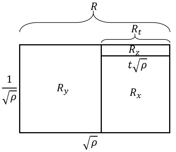
Figure 2: Rectangle instance of Case 1 in the proof of approximation factor.

Case 1.1 First, we show that if $z\geq 0.01$, the approximation factor is less than 1.19. We need to show that

$$\max\,\frac{\sqrt{\rho}+t\sqrt{\rho}+2/\sqrt{\rho}+1.5z/\sqrt{\rho}\,t}{2(\sqrt{x}+\sqrt{z}+\sqrt{1-t})}\leq 1.19$$

s.t.

$$1\leq\rho\leq 3$$

$$x+z=t$$

$$y+t=1$$

$$\rho>\frac{z}{t^{2}}$$

$$\rho\geq\frac{1}{3t}$$

$$\rho\leq\frac{1}{t}$$

$$1-t\geq x(=t-z)$$

Where inequalities state the range of rectangle $R,R_{t}$ and $R_{z}$ aspect ratios. We also have $z\geq 0.01$.

Proof of the bound:
Replacing $x$ with $t-z$ we need to show that:

The second derivative of the expression over $z$ is:

$$\frac{-0.595}{\sqrt{z^{3}}}-\frac{0.595}{\sqrt{(t-z)^{3}}}<0$$

Therefore, minimum of expression is either at $z=\max\{0.01,2t-1\}$ or at $z=\frac{\rho t^{2}}{3}$.

$\bm{z=0.01\;(2t-1\leq 0.01):}$ We need to show that:

Second derivative over $t$ is always negative. Then, $t=\frac{1}{3\rho}$ or $t=\min\{\frac{1}{\rho},0.505\}$.

• $t=0.505:$ We want to show that:

  The left hand side is always positive for $1\leq\rho\leq 1/0.505$.

• $t=\frac{1}{\rho}:$ We want to show that:

  The left hand side is always positive for $1/0.505\leq\rho\leq 3$.

• $t=\frac{1}{3\rho}:$ We want to show that:

  which holds for all $1\leq\rho\leq 3$.
  

$\bm{z=2t-1\;(0.01\leq 2t-1):}$ We need to show that:

$$4.76\sqrt{1-t}+2.38\sqrt{2t-1}-\sqrt{\rho}-t\sqrt{\rho}-\frac{5}{\sqrt{\rho}}+\frac{1.5}{\sqrt{\rho}t}\geq 0$$

The second derivative over $t$ is:

$$\frac{d^{2}}{dt^{2}}=\frac{-1.19}{\sqrt{(1-t)^{3}}}+\frac{3}{t^{3}\sqrt{\rho}}-\frac{2.38}{\sqrt{(2t-1)^{3}}}\,,$$

which is always negative for $\rho=1$ and consequently for all $\rho$’s greater than $1$. Hence minimum occurs in $t=0.505,t=\min(\frac{1}{\rho},\frac{3-3\sqrt{1-\rho/3}}{\rho})$. $\frac{3-3\sqrt{1-\rho/3}}{\rho}$ comes from the fact that $2t-1\leq\rho t^{2}/3$. For $t=0.505,z=2t-1=0.01$ which is investigated before. For other cases we can easily see that the expression is always positive.

$\bm{z=\frac{\rho t^{2}}{3}:}$ Replacing $z$ into the expression we need to show that:

The minimum of this expression for $1\leq\rho\leq 3$ and $\frac{1}{9}\leq t\leq 0.6$ is in $\rho=1$ and $t=0.6$ which is 0.56. Hence, it is always positive.

Case 1.2 Now we want to show that for $z<0.01$ the approximation factor also holds. To show that, we need some other lemmas.

Lemma 8.

For case 1 without considering other rectangles, the approximation factor is bounded by $0.75\sqrt{\rho/2}+\sqrt{1/2\rho}$ for $1\leq\rho\leq 2$.

Proof.

We need to show that

$$\max\frac{\sqrt{\rho}+t\sqrt{\rho}+2/\sqrt{\rho}+1.5z/t\sqrt{\rho}}{2(\sqrt{t-z}+\sqrt{z}+\sqrt{1-t})}\leq 0.75\sqrt{\frac{\rho}{2}}+\sqrt{\frac{1}{2\rho}}$$

or

$$\sqrt{2\rho}(1+t)+\frac{2\sqrt{2}}{\rho}+\frac{3z}{t\sqrt{2\rho}}\\ -(1.5\sqrt{\rho}+\frac{2}{\sqrt{\rho}})(\sqrt{t-z}+\sqrt{z}+\sqrt{1-t})\leq 0$$

s.t.

$$z\geq\max\{0,2t-1\}$$

$$z\leq\rho t^{2}/3$$

$$\frac{1}{3\rho}\leq t\leq\frac{1}{\rho}$$

$$\frac{d^{2}}{dz^{2}}=(1.5\sqrt{\rho}+\frac{2}{\sqrt{\rho}})(\frac{1}{4\sqrt{z^{3}}}+\frac{1}{4\sqrt{(t-z)^{3}}})\geq 0$$

Hence, $z=\max(0,2t-1)$ or $z=\rho t^{2}/3$.

If $2t-1\leq 0:$ In this case, $z=0$. The expression would become:

$$\sqrt{2\rho}(1+t)+\frac{2\sqrt{2}}{\sqrt{\rho}}-(1.5\sqrt{\rho}+\frac{2}{\sqrt{\rho}})(\sqrt{t}+\sqrt{1-t})$$

The maximum of this expression for $\rho\in\bigg{[}1,2\bigg{]}$ and $t\in\bigg{[}\frac{1}{3\rho},0.5\bigg{]}$ is in $t=0.5$ which is equal to 0.

If $2t-1\geq 0:$ In this case, $z=2t-1$. The expression would become:

Again, maximum of this expression for defined intervals of $\rho$ and $t$ is in $t=0.5$ which is equal to 0.

If $z=\rho t^{2}/3$: The expression would become:

Here, $t\in\bigg{[}\frac{1}{3\rho},\min\{\frac{1}{\rho},\frac{3-\sqrt{9-3\rho}}{\rho}\}\bigg{]}$. This comes from substituting $z$ in $y=1-t\geq t-z$. Hence, the approximation factor is maximized when $t=0.5$ and $z=0$ for $1\leq\rho\leq 2$. ∎

Lemma 9.

For Case 1 without considering other rectangles, the approximation factor is bounded by $\frac{3+\rho}{2+2\sqrt{\rho-1}}$ for $2\leq\rho\leq 3$.

Proof.

We need to show that

$$\max\frac{\sqrt{\rho}+t\sqrt{\rho}+2/\sqrt{\rho}+1.5z/t\sqrt{\rho}}{2(\sqrt{t-z}+\sqrt{z}+\sqrt{1-t})}\leq\frac{3+\rho}{2+2\sqrt{\rho-1}}$$

or

$$(\frac{2}{\sqrt{\rho}}+\sqrt{\rho}(1+t)+\frac{1.5z}{t\sqrt{\rho}})(\frac{1}{\sqrt{\rho}}+\sqrt{1-\frac{1}{\rho}})\\ -(\sqrt{\rho}+\frac{3}{\sqrt{\rho}})(\sqrt{t-z}+\sqrt{z}+\sqrt{1-t})\leq 0$$

s.t.

$$z\leq\frac{\rho t^{2}}{3}$$

$$\frac{1}{3}\leq t\leq\frac{1}{\rho}$$

$$\frac{d^{2}}{dz^{2}}=(\sqrt{\rho}+\frac{3}{\sqrt{\rho}})(\frac{1}{4\sqrt{z^{3}}}+\frac{1}{4\sqrt{(t-z)^{3}}})\geq 0$$

Hence, $z=0$ or $z=\rho t^{2}/3$.

$\bm{z=0:}$ In this case, The expression becomes:

$$(\sqrt{\rho}(1+t)+\frac{2}{\sqrt{\rho}}+\frac{t\sqrt{\rho}}{2})(\frac{1}{\sqrt{\rho}}+\sqrt{1-\frac{1}{\rho}})\\ -(\sqrt{\rho}+\frac{3}{\sqrt{\rho}})(t\sqrt{\frac{\rho}{3}}+\sqrt{1-t}+\sqrt{t-\frac{t^{2}\rho}{3}})$$

The maximum of this expression for $\rho\in\bigg{[}2,3\bigg{]}$ and $t\in\bigg{[}\frac{1}{3},\frac{1}{\rho}\bigg{]}$ is in $t=\frac{1}{3}$, $\rho=3$ which is equal to 0.

$\bm{z=\rho t^{2}/3}$: The expression would become:

The maximum of this expression occurs in $t=\frac{1}{3}$ and $\rho=\frac{1}{3}$ which is $-0.3853<0$.
Hence, the approximation factor is maximized when $z=0$ and $t=1/\rho$ for $2\leq\rho\leq 3$. ∎

For Case 1 if rectangle $R$ in Figure 2 is not the main rectangle that we intend to partition, It must have a parent and a sibling. We call the sibling $R^{\prime}$. $R^{\prime}$ would locate at the bottom/ top of rectangle $R$ or at the left/right side of that. We need to know how many children $R^{\prime}$ has. First we show that it is either a simple rectangle or has up to four children. First, remember that we sort the list of areas in descending order. We have $R_{y}$, $R_{x}$ and $R_{z}$ with areas $y$, $x$ and $z$ respectively. We know that $y\geq x\geq z$ and $x$ and $z$ are located at the end of the list of areas and the would sum up and will locate in new ordered list of areas. We know that before summing $x+z$ and $y$ together (Before they locate at the end of the list) several double areas could get summed together. We know that they make new areas greater than $x+z$. Making new areas from areas smaller than $x+z$ and $y$ by summing up them in pairs continues until $x+z$ and $y$ be located at the end of the list. Now they will be summed (equal to 1) and relocate in the list. Now in the list there might be one single and several paired areas or just several paired areas after $x+y+z$. Then these area ahead of $x+y+z$ get summed while we know that their summation is greater than $x+y+z=1$. This continues until it is time for $x+y+z$ to get summed with another area, while we know that the current areas in the list are consisted from at most 4 areas from the original list.
Here we separate the discussion into two cases; when $R^{\prime}$ is a simple rectangle and when it a compound rectangle.

$\bm{R^{\prime}}$ is a compound rectangle: Suppose that $R^{\prime}$ is a compound rectangle containing 2, 3 or 4 sub-rectangles. Moreover, since when $x+z$ and $y$ locate at the end of the list, the area of combinations of two areas which are located before $x+z$ and $y$ is greater than $\max\{2x,y\}$, considering it with $z\leq\frac{x}{2}$ results in $a_{i},a_{i-1}\geq x\geq\frac{2}{7}$. Also, the area of $R\prime$ cannot be greater than 2. Because when $y$ and $x+z$ are summed there are two areas in the list ahead of them with area less than $x+y+x=1$ which are children of $R\prime$ (consisting single or double area). If $R^{\prime}$ locate at the bottom/top of rectangle $R$ we know that there are at least two sub-rectangle in them each having area greater than $x$ and less than $x+z$. Remember that $z<0.01$ and these two sub-rectangles hence the areas of these two are very close. We claim that these two sub-rectangles together has $AR\leq 3$. It is not hard to show it using lemma 2 since we know that the AR of rectangle $R$ parent is less than 3 and the area of all sub-rectangles inside $R\prime$ are very close in case of 2 and 4 sub-rectangles because all of them are less than $x+z$ and greater than $x$. In the case of 3 sub-rectangles assume that before having 3 sub-areas $a_{0}$ is the single child of $R\prime$ and $a_{1}$ and $a_{2}$ are the ones which are summed together. So, at some point the list was:

$$...,a_{0},x+z,y,a_{1},a_{2}$$

Note that the order of $x+z$ and $y$ could be switched.

$$...,a_{0},a_{1}+a_{2},x+z,y$$

Again in addition to order of $x+z$ and $y$ the order of $a_{0}$ and $a_{1}+a_{2}$ could be switched. Then the list will be updated to

$$...,x+z+y,a_{0},a_{1}+a_{2}\,,$$

and then

$$...,a_{0}+a_{1}+a_{2},x+z+y\,,$$

where finally $x+z+y$ is getting summed with these three sub-areas. Hence, in the case that $a_{0}$ is less than $a_{1}+a_{2}$, $a_{0}\geq\max\{x+z,y\}\geq 0.5$ and $a_{1}+a_{2}\leq 1$. Hence the AR of $a_{0}$ and compound rectangle having $a_{1}+a_{2}$ is less than 3. In the case that $a_{0}$ is greater than $a_{1}+a_{2}$, $a_{0}\leq 1$ and $a_{1}+a_{2}\geq\max\{2x,y\}$ which knowing that $z\leq 0.01$ results in $a_{1}+a_{2}\geq 0.66$. Thus again the AR of $a_{0}$ and compound rectangle having $a_{1}+a_{2}$ is less than 3. The same result holds for when $R^{\prime}$ would locate at the right/left side of rectangle $R$, because these two sub-rectangles always have area less than $x+y+z=1$ and hence the AR of $R$ containing $x,y,z$ is less than 3, the AR of the rectangle containing these two sub-rectangles is also less than 3.
As we showed what we claimed now based on the fact that the area of two sub-rectangles are very close the AR of the bigger one is always less than 2 and the other one less than 3. Moreover, we know that each of them has an area greater than $0.33$.

$\bm{R^{\prime}}$ is a simple rectangle: $R^{\prime}$ is a simple rectangle, its area is greater than $\max\{x+z,y\}$ and hence greater than 0.5. If it is not a forced simple rectangle the AR of $R$ and $R^{\prime}$ together must be less than 3, since otherwise,it would be defined as $z$. If $R^{\prime}$ is at the bottom/top the worst AR happens when $\rho=1.5$ and $a_{R^{\prime}}=0.5$ and the AR is 3. That is because in order to have $R^{\prime}$ at the top/bottom of $R$ and not at the right/left side of it the height of parent of $R$ and $R^{\prime}$ should be greater than $\sqrt{\rho}$ which is the width and hence the AR of $R^{\prime}$ in the case of its width is greater than its height, is $\frac{\sqrt{\rho}}{\sqrt{\rho}-\frac{1}{\sqrt{\rho}}}$. Therefore, the area should be greater than $\sqrt{\rho}(\sqrt{\rho}-\frac{1}{\sqrt{\rho}})=\rho-1$ Together with area greater than 0.5, we know that areas should be greater than $\max\{0.5,\rho-1\}$. On the other hand, since the AR of $R$ and $R^{\prime}$ together should not be greater than 3, the area of $R^{\prime}$ should be less than $3\rho-1$.
In the situation that $R^{\prime}$ is at the left/right side of $R$, if the area of $R^{\prime}$ is $A_{R}^{\prime}$ its AR should be $\rho A_{R}^{\prime}$ in a way that overall AR of $R$ and $R^{\prime}$ stay under 3, i.e., $A_{R^{\prime}}\leq 3/\rho-1$.
Now suppose that $R^{\prime}$ is a forced rectangle, in this case its area is greater than 1 and as a result in approximation factor calculation we can use the lower bound of $w+h$. Clearly, this lower bound reduces the overall approximation factor more than having a rectangle with area $A_{R}^{\prime}$ AR of $\rho A_{R}^{\prime}$ while the overall AR of $R$ and $R^{\prime}$ stay under 3.

Lemma 10.

If Rectangle $R$ in Case 1 (Figure 2) is not the main rectangle that we want to partition the approximation factor of Algorithm 1 is 1.203.

Proof.

By lemma 2.8.4 and 2.8.5 we have the approximation factors of rectangle $R$ in case 1 without considering extra rectangles. Now we consider sub-rectangles in $R^{\prime}$ in the calculation of approximation factor. First for the case that $R^{\prime}$ is not simple. We showed that there are at least two sub-rectangles in $R^{\prime}$ that has area greater than 0.33 and one of them $AR\leq 2$ and the other $AR\leq 3$. We include them to the approximation factors we had. For $1\leq\rho\leq 2$ it will be:

$$\frac{1.5\sqrt{\rho}+\frac{2}{\sqrt{\rho}}+4\sqrt{0.11}+3\sqrt{0.165}}{2\sqrt{2}+4\sqrt{0.33}}$$

$4\sqrt{0.11}+3\sqrt{0.165}$ comes from putting $wh=0.33$ and $w/h=3$ and $w/h=2$ respectively. The expression is maximized for $\rho=2$ and the value is 1.1862. For $2\leq\rho\leq 3$ it will be:

$$\frac{\sqrt{\rho}+\frac{3}{\sqrt{\rho}}+4\sqrt{0.11}+3\sqrt{0.165}}{2(\frac{1}{\sqrt{\rho}}+\sqrt{1-\frac{1}{\rho}})+4\sqrt{0.33}}$$

This is maximized for $\rho=2$ and the value is 1.1863.
Now suppose that $R^{\prime}$ is a simple rectangle at the left/right of $R$ then $0.5\leq A_{R^{\prime}}\leq 3/\rho-1$ the approximation factor would be

$$\frac{1.5\sqrt{\rho}+\frac{2}{\sqrt{\rho}}+A_{R^{\prime}}\sqrt{\rho}+\frac{1}{\sqrt{\rho}}}{2\sqrt{2}+2\sqrt{A_{R^{\prime}}}}$$

Note that since $0.5\leq 3/\rho-1$, obviously $\rho\leq 2$ and we do not need approximation factor for $\rho\geq 2$ The maximum of this expression is 1.2029 for $\rho=1.5$ and $A_{R^{\prime}}=0.5$
Now suppose that $R^{\prime}$ is a simple rectangle at the top/bottom of $R$ then $\max\{0.5,\rho-1\}\leq A_{R^{\prime}}\leq 3\rho-1$ the approximation factor would be

$$\frac{1.5\sqrt{\rho}+\frac{2}{\sqrt{\rho}}+\sqrt{\rho}+\frac{A_{R^{\prime}}}{\sqrt{\rho}}}{2\sqrt{2}+2\sqrt{A_{R^{\prime}}}}$$

for $1\leq\rho\leq 2$ and

$$\frac{\sqrt{\rho}+\frac{3}{\sqrt{\rho}}+\sqrt{\rho}+\frac{A_{R^{\prime}}}{\sqrt{\rho}}}{2(\frac{1}{\sqrt{\rho}}+\sqrt{1-\frac{1}{\rho}})+2\sqrt{A_{R^{\prime}}}}$$

for $2\leq\rho\leq 3$. The maximum of these expressions on the defined intervals is 1.2029 for $\rho=1.5$ and $A_{R^{\prime}}=0.5$. ∎

Case 2 Consider a rectangle R with aspect ratio $(\rho)$ less than 3 which is dissected into two rectangles $R_{y}$ which is a simple rectangle and $R_{t}$ which is a compound rectangle having aspect ratio less than 3 consisting a simple rectangle as its left child $(R_{x})$ and $R_{z}$ as its right child which can be either a compound or a simple rectangle and $R_{z}$ is located at the right side of $R_{x}$. For simplicity, suppose that area of R is 1 and its width is greater than its height (Figure 3)

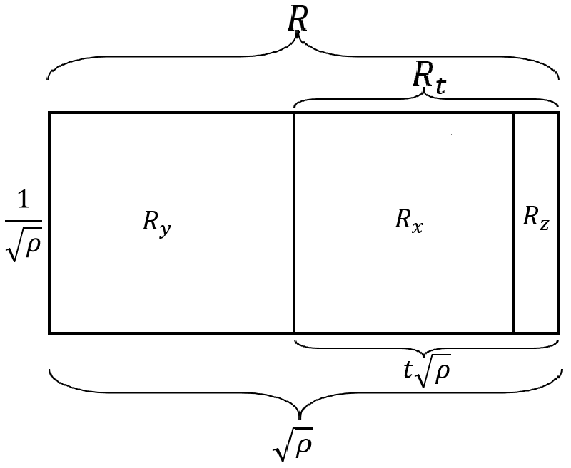
Figure 3: Rectangle instnace of Case 2 in the proof of approximation factor.

We will show that the worst state of this case is equivalent to the worst case of Case 1 and hence everything we proved for Case 1 also holds here. Therefore, we need to show that the approximation factor in this case is less than $\frac{\frac{3}{\sqrt{\rho}}+\sqrt{\rho}}{2(\sqrt{\frac{1}{\rho}}+\sqrt{1-\frac{1}{\rho}})}$ for $2\leq\rho\leq 3$, i.e.,

$$\frac{\frac{3}{\sqrt{\rho}}+\sqrt{\rho}+1.5\sqrt{\rho}z}{2(\sqrt{t-z}+\sqrt{1-t}+\sqrt{z})}\leq\frac{\frac{3}{\sqrt{\rho}}+\sqrt{\rho}}{2(\sqrt{\frac{1}{\rho}}+\sqrt{1-\frac{1}{\rho}})}$$

or

$$(\frac{3}{\sqrt{\rho}}+\sqrt{\rho}+1.5\sqrt{\rho}z)(\sqrt{\frac{1}{\rho}}+\sqrt{1-\frac{1}{\rho}})\\ -(\frac{3}{\sqrt{\rho}}+\sqrt{\rho})(\sqrt{t-z}+\sqrt{1-t}+\sqrt{z})\leq 0$$

s.t.

$$z\leq\frac{1}{3\rho},$$

$$t\geq\frac{1}{\rho},$$

$$z\geq 2t-1$$

$$\frac{d^{2}}{dz^{2}}=(\frac{1}{4\sqrt{(t-z)^{3}}}+\frac{1}{4\sqrt{z^{3}}})(\frac{3}{\sqrt{\rho}}+\sqrt{\rho})\geq 0$$

Hence, $z=\max\{0,2t-1\}$ or $z=\frac{1}{3\rho}$.

If $z=0:$ The expression will be

$$(\frac{3}{\sqrt{\rho}}+\sqrt{\rho})(\frac{1}{\sqrt{\rho}}+\sqrt{1-\frac{1}{\rho}}-\sqrt{t}-\sqrt{1-t})$$

Since $t\geq\frac{1}{\rho}$, the expression is always negative.

If $z=2t-1:$ The expression will be

$$(\frac{3}{\sqrt{\rho}}+\sqrt{\rho}+1.5\sqrt{\rho}(2t-1))(\frac{1}{\sqrt{\rho}}+\sqrt{1-\frac{1}{p}})\\ -(\frac{3}{\sqrt{\rho}}+\sqrt{\rho})(\sqrt{2t-1}+2\sqrt{1-t})$$

Clearly, $\frac{d^{2}}{dt^{2}}\geq 0$ and the maximum value of the expression is in $t=0.5$ or $t=0.6$ (because $t\leq 0.6$), In $t=0.5$ the maximum value of expression is 0 and for $t=0.6$ it is -0.378.
If $z=\frac{1}{3\rho}:$ The expression will be

$$(\frac{3}{\sqrt{\rho}}+\sqrt{\rho}+\frac{1.5}{\sqrt{3\rho}})(\frac{1}{\sqrt{\rho}}+\sqrt{1-\frac{1}{p}})\\ -(\frac{3}{\sqrt{\rho}}+\sqrt{\rho})(\sqrt{\frac{1}{3\rho}}+\sqrt{t-\frac{1}{3\rho}}+\sqrt{1-t})$$

Since $\frac{d^{2}}{dt^{2}}\geq 0$, either $t=\frac{1}{\rho}$ or $t=\frac{1}{2}+\frac{1}{6\rho}$ which has a maximum of $-0.1417$ in $\rho=3$.

If $\rho\leq 2$ we need to show that:

$$\frac{\frac{3}{\sqrt{\rho}}+\sqrt{\rho}+1.5\sqrt{\rho}z}{2(\sqrt{t-z}+\sqrt{1-t}+\sqrt{z})}\leq 0.75\sqrt{\frac{\rho}{2}}+\sqrt{\frac{1}{2\rho}}$$

or

$$\sqrt{2}(\frac{3}{\sqrt{\rho}}+\sqrt{\rho}+.5z\sqrt{\rho})\\ -(1.5\sqrt{\rho}+\frac{2}{\sqrt{\rho}})(\sqrt{z}+\sqrt{t-z}+\sqrt{1-t})\leq 0$$

s.t

$$z\geq\max\{0,2t-1\}$$

$$z\leq 1/3\rho$$

$$\frac{1}{\rho}\leq t\leq 0.5+0.5z$$

Since $\frac{d^{2}}{dz^{2}}\geq 0$, either $z=\max\{0,2t-1\}$ or $z=\frac{1}{3\rho}$.

If $z=0$: The only valid value for $\rho$ is 2 and it is similar to previous analysis.

If $z=2t-1:$

Clearly, $\frac{d^{2}}{dt^{2}}\geq 0$ and the maximum value of the expression is in $t=0.5$ or $t=0.6$ (because $t\leq 0.6$), In $t=0.5$ the maximum value of expression is 0 and for $t=0.6$ it is -0.45.
If $z=\frac{1}{3\rho}:$ The expression would be

Since $\frac{d^{2}}{dt^{2}}\geq 0$, either $t=\frac{1}{\rho}$ or $t=\frac{1}{2}+\frac{1}{6\rho}$ which have a maximum of $-0.13$ in $\rho=5/3$. Note that $\rho\geq 5/3$.

Case 3: Consider a rectangle R with aspect ratio $(\rho)$ less than 3 which is dissected into two rectangles $R_{y}$ which is a compound rectangle consisting rectangles $y_{1}$ and $y_{2}$ divided horizontally and $R_{t}$ which is a compound rectangle having aspect ratio less than 3 consisting two rectangles $R_{x}$ and $R_{z}$ (such as case 1) divided horizontally. For simplicity, suppose that area of $R$ is 1 and its width is greater than its height (Figure 4).

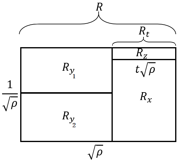
Figure 4: Rectangle instance of Case 3 in the proof of approximation factor.

For this case to be generated, at some point the list is like

$$...,y_{1},y_{2},x,z,$$

then

$$...,x+z,y_{1},y_{2}$$

and

$$...,y_{1}+y_{2},x+z$$

Therefore, we know that $x+z\geq y_{1}\geq y_{2}\geq x$

$$y_{1}+y_{2}\geq 2x\Rightarrow 2(t-z)\leq 1-t\Rightarrow z\geq 1.5t-0.5$$

Moreover,

$$\frac{\rho t^{2}}{z}\geq 3\Rightarrow z\leq\frac{\rho t^{2}}{3}$$

We also have

$$\frac{1}{\sqrt{\rho}}\geq\sqrt{\rho}(1-t)\Rightarrow t\geq 1-\frac{1}{\rho}$$

On the other hand,

$$t\sqrt{\rho}\leq\frac{1}{\sqrt{\rho}}\Rightarrow t\leq\frac{1}{\rho}$$

We show that the approximation factor for this case is less than 1.2.

$$\frac{2\sqrt{\rho}+\frac{2}{\sqrt{\rho}}+\frac{1.5z}{t\sqrt{\rho}}}{2(\sqrt{t-z}+\sqrt{z}+\sqrt{y_{1}}+\sqrt{y_{2}})}\leq 1.2$$

We know that $y_{1}+y_{2}=1-t$. In this situation the minimum of them occurs when $y_{1}$ and $y_{2}$ are extremely different from each other. Thus, here that we have $y_{2}\geq x$ the minimum is in $y_{2}=x$ and $y_{1}=1-t-y_{2}=1-t-t+z=1-2t+z$ So we need to show that

$$2\sqrt{\rho}+\frac{2}{\rho}+\frac{1.5z}{t\sqrt{\rho}}-2.4(2\sqrt{t-z}+\sqrt{z}+\sqrt{1-2t+z})\leq 0$$

$$\frac{d^{2}}{d\rho^{2}}=-\frac{1}{2\sqrt{\rho^{3}}}+\frac{3}{2\rho^{2}\sqrt{\rho}}+\frac{9z}{8t\rho^{2}\sqrt{\rho}}\geq 0$$

Hence, either $\rho=1$ or $\rho=\min\{\frac{1}{t},\frac{1}{1-t}\}=\frac{1}{1-t}$.

If $\rho=1:$ The expression will be

$$4+\frac{1.5z}{t}-2.4(2\sqrt{t-z}+\sqrt{z}+\sqrt{1-2t+z})$$

For this expression we have $\frac{d^{2}}{dz^{2}}\geq 0$ and the maximum is either $z=1.5t-0.5$ or $z=\frac{\rho t^{2}}{3}$.

If $z=1.5t-0.5:$ Replacing $z$ with $1.5t-0.5$ for $\frac{1}{3}\geq t,$ we have the maximum in $t=\frac{1}{3}$ which is -0.1569.

If $z=\frac{\rho t^{2}}{3}:$ Replacing $z$ with $z=\frac{\rho t^{2}}{3}$ for $t\leq 0.36255$ the minimum of expression is in the extreme point of $t$ and is -0.3859. Note that the interval for $t$ in this case is defined by replacing $z$ by $\frac{\rho t^{2}}{3}$ in $z\geq 1.5t-0.5$.

Now if $\rho=\frac{1}{1-t}$: The expression would become

Second derivative of this over $z$ is positive and the maximum of expression would be on the extreme points, $z=1.5t-0.5$ or $z=\frac{\rho t^{2}}{3}=\frac{t^{2}}{3-3t}$. Replacing $z$ with both of these values results in the maximum of expression in $t=\frac{1}{3}$ with negative values -0.0744 and -0.3055 respectively.

Case 4 This case is similar to case 3 with the difference that $y_{1}$ and $y_{2}$ are divided with a vertical line. (Figure 5)

Figure 5: Rectangle instance of Case 4 in the proof of approximation factor.

So, we need to show that:

$$\frac{\frac{3}{\sqrt{\rho}}+\sqrt{\rho}+t\sqrt{\rho}+\frac{1.5z}{t\sqrt{\rho}}}{2(\sqrt{z}+2\sqrt{t-z}+\sqrt{1-2t+z})}\leq 1.2$$

or

s.t.

$$1-t\geq\frac{1}{\rho}\geq t$$

and

$$1.5t-0.5\leq z\leq\frac{\rho t^{2}}{3}$$

Since we know that

$$\frac{d^{2}}{d\rho^{2}}=\frac{1}{4\rho^{2}\sqrt{\rho}}(-\rho-t\rho+9+\frac{4.5z}{t})\geq 0$$

, we will have $\rho=\frac{1}{t}$ or $\rho=\frac{1}{1-t}$.

If $\rho=\frac{1}{t}$: The expression will be

$$\frac{1}{\sqrt{t}}+4\sqrt{t}+\frac{1.5z}{\sqrt{t}}-2.4(\sqrt{z}+2\sqrt{t-z}+\sqrt{1-2t+z})$$

Since second derivative of the expression over $z$ is always positive, $z=\frac{\rho t^{2}}{3}$ or $z=1.5t-0.5$.

If $z=\frac{\rho t^{2}}{3}=\frac{t}{3}:$ The expression will be

$$\frac{1}{\sqrt{t}}+4.5\sqrt{t}-2.4(\sqrt{\frac{t}{3}}+2\sqrt{\frac{2t}{3}}+\sqrt{1-\frac{5t}{3}})$$

This expression is negative for any number in $[0.17,0.54]$ which includes $t$.

If $z=1.5t-0.5$ the expression is:

$$\frac{0.25}{\sqrt{t}}+6.25\sqrt{t}-2.4(\sqrt{1.5t-0.5}+3\sqrt{0.5-0.5t})$$

which is negative for $[1/3,0.54].$

If $\rho=\frac{1}{1-t}$: The expression will be

$$\frac{1}{\sqrt{t}}+4\sqrt{t}+\frac{1.5z}{\sqrt{t}}-2.4(\sqrt{z}+2\sqrt{t-z}+\sqrt{1-2t+z})$$

Similar to previous expression replacing $\rho=\frac{1}{1-t}$ and taking derivative over $z$, the value of derivative is always positive which results in $z=\frac{\rho t^{2}}{3}$ or $z=1.5t-0.5$. Replacing them in the expression again results in only negative values for expression.

Case 5 Consider a rectangle $R$ with aspect ratio ($\rho$) greater than 3 which is dissected into two rectangles $R_{y}$ which is a simple rectangle and $R_{t}$ which is a compound rectangle having aspect ratio less than 3 consisting a simple rectangle as its left child ($R_{x}$) and $R_{z}$ as its right child which can be either a compound or a simple rectangle and $R_{z}$ is located on top of $R_{x}$. For simplicity, suppose that area of $R$ is 1 and its width is greater than its height (Figure 6).

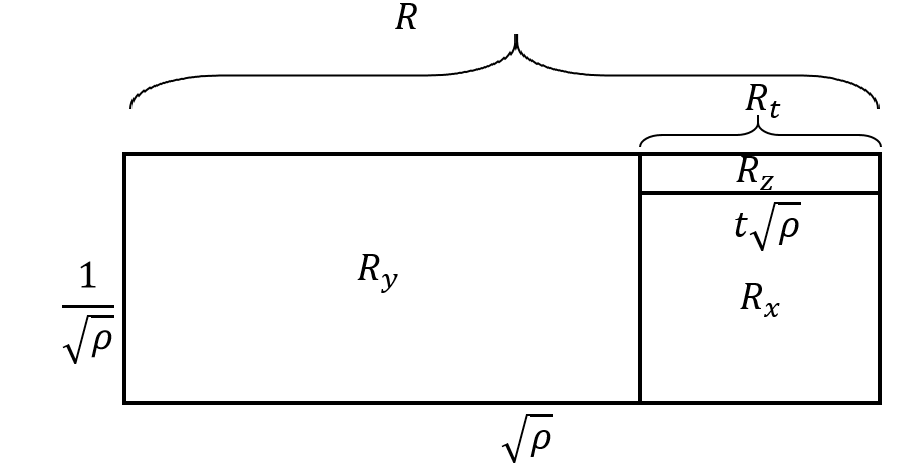
Figure 6: Rectangle instnace of Case 5 in the proof of approximation factor.

In this case, where we have $\rho\geq 3$, either $R$ should have belonged to $z$ or $R$ is part of $R_{0}$. If former happens we are done, but if latter happens we need to show that the approximation factor is less than $1.2$ or

$$\frac{\sqrt{\rho}+t\sqrt{\rho}+\frac{2}{\sqrt{\rho}}+\frac{1.5z}{t\sqrt{\rho}}}{2(\sqrt{z}+\sqrt{t-z})+\sqrt{\rho}(1-t)+\frac{1}{\sqrt{\rho}}}\leq 1.2$$

or

subject ot the constraints be fulfilled. Since second derivative over $z$ is always positive, $z=0$ or $z=\frac{\rho t^{2}}{3}$.

If $z=0$: The expression becomes

$$\sqrt{\rho}+t\sqrt{\rho}+\frac{2}{\sqrt{\rho}}-1.2(2\sqrt{t}+\sqrt{\rho}(1-t)+\frac{1}{\sqrt{\rho}})$$

Here, second derivative over $t$ is always positive. Hence, $t=\frac{1}{\rho}$ or $t=\frac{1}{3\rho}$.

If $t=\frac{1}{\rho}$:

$$\frac{0.6}{\sqrt{\rho}}-0.2\sqrt{\rho}$$

For $\rho\geq 3$ maximum of this expression is equal to 0 at $\rho=3$.

If $t=\frac{1}{3\rho}$:

$$\frac{4.6}{3\sqrt{\rho}}-0.2\sqrt{\rho}-\frac{2.4}{\sqrt{3\rho}}$$

For $\rho\geq 3$ maximum of this expression is equal to -0.26 at $\rho=3$.

If $z=\frac{\rho t^{2}}{3}$: The expression will be

The value of this expression on defined intervals is on $\rho=3$ which is -0.38.

Case 6 Consider a rectangle $R$ with aspect ratio ($\rho$) greater than 3 which is dissected into two rectangles $R_{y}$ which is a simple rectangle and $R_{t}$ which is a compound rectangle having aspect ratio less than 3 consisting a simple rectangle as its left child ($R_{x}$) and $R_{z}$ as its right child which can be either a compound or a simple rectangle and $R_{z}$ is located at the right side of $R_{x}$. For simplicity, suppose that area of $R$ is 1 and its width is greater than its height (Figure 7).

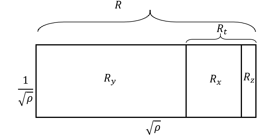
Figure 7: Rectangle instance of Case 6 in the proof of approximation factor.

Similar to Case 5, we have $\rho\geq 3$ and, either $R$ should have belonged to $z$ or $R$ is part of $R_{0}$. If former happens we are done, but if latter happens, $R_{y}$ would be a part of main rectangle. The proves for case 2 also holds here and the worst case of this case is similar to worst case of case 5 which we showed the approximation factor is less than 1.2.

Case 7 Suppose that $R_{0}$ is a rectangle with aspect ratio ($\rho$) which using our approximation algorithm is dissected into two rectangles $R_{x}$ which is a simple rectangle and $R_{z}$ which is either a simple or compound rectangle and $R_{x}$ and $R_{z}$ are divided by a vertical line. For simplicity, suppose that area of $R$ is 1 and its width is greater than its height (Figure 8 ).

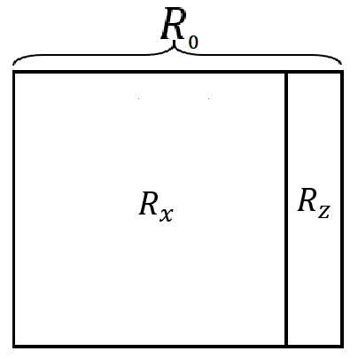
Figure 8: Rectangle instance of Case 7 in the proof of approximation factor.

In this case, if width of $R_{x}$ is greater than its height it would be a forced rectangle. On the other hand most part of $R_{z}$ is composed of either forced rectangles or rectangles with aspect ratio less than 3. The reason behind this is that either height of those rectangles are greater than their width or unless the very end of the area list the rectangles that are generated inside $z$ in the middle steps have $AR\leq 3$. Hence, in the worst case we can consider the big portion of $z$ has $AR=3$ and a small portion has $AR>3$ which is not a forced rectangle and may include some sub-rectangles.
To do that we separate these two parts. The small portion cannot have an area greater than $\frac{z^{2}\rho}{3}$ since its AR should be greater than 3 (Figure 9).

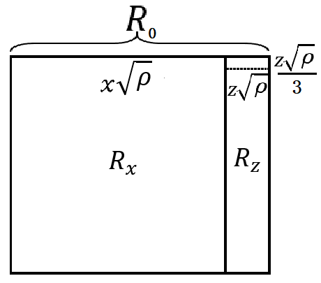
Figure 9: Rectangle mentioned in Case 7 in the proof of approximation factor

As a result the rest area of $R_{z}$ is greater than $z-\frac{z^{2}\rho}{3}$. Considering all this part consisting sub-rectangles with $AR=3$, we can ignore them because they only have positive contribution in compensating for the small section of $R_{z}$ with aspect ratio more than 3. The upper bound of smaller area is $z\sqrt{\rho}+z\frac{\sqrt{\rho}}{3}+1.5\frac{z\sqrt{\rho}}{3}=\frac{5.5z\sqrt{\rho}}{3}$. First assume that width of $R_{x}$ is greater than its height. In this situation It is enough to show that:

$$\frac{x\sqrt{\rho}+\frac{1}{\sqrt{\rho}}+\frac{5.5z\sqrt{\rho}}{3}}{x\sqrt{\rho}+\frac{1}{\sqrt{\rho}}+\frac{2z\sqrt{\rho}}{\sqrt{3}}}\leq 1.2$$

s.t.

$$z\leq\frac{1}{3\rho},$$

$$z\leq 1-\frac{1}{\rho}$$

First constraint refers to the lower bound of 3 for aspect ratio of $R_{z}$ and second constraint ensures that $R_{x}$ is a forced rectangle. So, we need to show that

The maximum of this expression is -0.2171 in $\rho=4/3$ and $z=0.25$.

Now assume that width of $R_{x}$ is less than its height. In this situation it is enough to show that:

$$\frac{x\sqrt{\rho}+\frac{1}{\sqrt{\rho}}+\frac{5.5z\sqrt{\rho}}{3}}{2\sqrt{x}+\frac{2z\sqrt{\rho}}{\sqrt{3}}}\leq 1.2$$

s.t.

$$z\leq\frac{1}{3\rho},$$

$$z>1-\frac{1}{\rho}$$

We want to show that

$$(1-z)\sqrt{\rho}+\frac{1}{\sqrt{\rho}}+\frac{5.5z\sqrt{\rho}}{3}-1.2(2\sqrt{1-z}+\frac{2z\sqrt{\rho}}{\sqrt{3}})\leq 0$$

The maximum of this expression is -0.2171 in $\rho=4/3$ and $z=0.25$.

Case 8 This case is similar to Case 1 (Figure 2) with the only difference that rectangle $R$ is the main rectangle that we want to partition($R_{0}$). For this case, either $R_{y}$ is a forced rectangle which causes $R_{x}$ to be a forced rectangle too or $R_{y}$ is not a forced rectangle. Similar to the analysis we did for case 7, when $R_{y}$ and $R_{x}$ are forced rectangle the approximation factor of whole $R$ is very low because only a very small part of $R_{z}$ may not be either a forced rectangle or a rectangle with AR less than 3. Thus we analyze for the situation that $R_{y}$ is not a forced rectangle.
Remember that a big proportion of $R_{z}$ is consist of sub-rectangles that either have width greater than height or has aspect ratio less than 3. The sub-rectangles that have larger width than height, we know that every other layout cause them to have bigger aspect ratios. (Figure 10) Hence again we disregard them and also the ones that have aspect ratio less than 3 in our calculation. The small part of $R_{z}$ that can be improved in other layouts has the maximum area of $\frac{z^{2}}{t\sqrt{3\rho}}$. Because it has $AR>3$ and height of $\frac{z}{\sqrt{\rho}t}$ and show that:

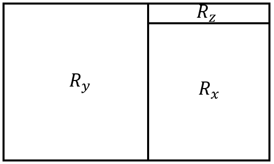
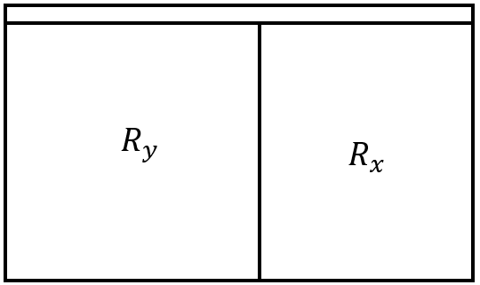
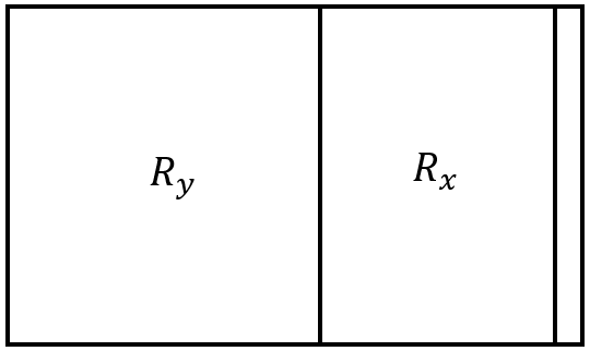
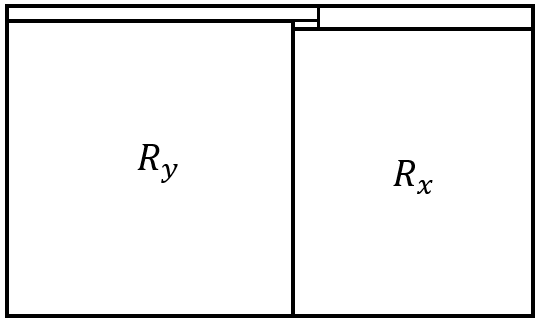
Figure 10: Four different sub-cases of Case 8 in the proof of approximation factor.

$$\frac{\sqrt{\rho}+\frac{2}{\rho}+\frac{z}{2t\sqrt{\rho}}}{2(\sqrt{y}+\sqrt{x}+\frac{z}{e\sqrt{3\rho}})}\leq 1.2$$

s.t.

$$t\geq 1-\frac{1}{\rho}$$

$$z<\frac{\rho t^{2}}{3}$$

$$t\geq\frac{1}{3\rho}$$

$$t\leq 0.5+0.5z$$

$$t\leq\frac{1}{\rho}$$

So, we need to prove

$$\sqrt{\rho}+\frac{2}{\sqrt{\rho}}+\frac{z}{2t\sqrt{\rho}}-2.4(\sqrt{1-t}+\sqrt{t-z}+\frac{z}{t\sqrt{3\rho}})\leq 0$$

Since second derivative of the expression over $z$ is always positive, $z=0$ or $z=\frac{\rho t^{2}}{3}$.

If $z=0$ the expression will be

$$\sqrt{\rho}+\frac{2}{\sqrt{\rho}}-2.4(\sqrt{1-t}+\sqrt{t})$$

From this we have either $t=\max\{\frac{1}{3\rho},1-\frac{1}{\rho}\}$ or $t=\min\{\frac{1}{\rho},0.5\}$.

If $t=\frac{1}{\rho}(\frac{1}{\rho}\leq 0.5)$: Since $1-\frac{1}{\rho}\leq\frac{1}{\rho}$, $\rho$ is bounded above by 2. So, $\rho=2$ is the only possible value for $\rho$ which makes the expression equal to -0.565.

If $t=\frac{1}{3\rho}(\frac{1}{3\rho}\geq 1-\frac{1}{\rho})$ The expression will be

$$\sqrt{\rho}+\frac{2}{\sqrt{\rho}}-2.4\sqrt{1-\frac{1}{3\rho}}-2.4\frac{1}{\sqrt{3\rho}}$$

The maximum of this expression for $1\leq\rho\leq 4/3$ would be on $\rho=1$ which is -0.34.

If $t=1-\frac{1}{\rho}(\frac{1}{3\rho}\leq 1-\frac{1}{\rho})$: The expression will be

$$\sqrt{\rho}+\frac{2}{\sqrt{\rho}}-2.4\sqrt{1-\frac{1}{\rho}}-\frac{2.4}{\sqrt{\rho}}$$

The maximum of this expression for $4/3\leq\rho\leq 2$ would be on $\rho=4/3$ which is -0.54.

If $z=\frac{\rho t^{2}}{3}$ the expression becomes

$$\sqrt{\rho}+\frac{2}{\sqrt{\rho}}+\frac{t\sqrt{\rho}}{6}-2.4(\sqrt{1-t}+\sqrt{t-\frac{\rho t^{2}}{3}}+\frac{t\sqrt{\rho}}{3\sqrt{3}})$$

The maximum of this is $-0.357$ on $t=0.6$ and $\rho=1$.

Case 9 This case is similar to Case 2 (Figure 3) with the only difference that rectangle R is the main rectangle that we want to partition($R_{0}$). The worst case of this case is similar to Case 8 and proves that the claim holds here too.

The following theorem summarizes our results.

Theorem 11.

Given a rectangle $R$ with $\mathop{\rm Area}\nolimits(R)=A$ and a list of areas $A_{1},...,A_{n}$ with $\sum_{i=1}^{n}A_{i}=A$, Algorithm 1 constructs a partition of $R$ into $n$ sub-rectangles with areas $A_{1},...,A_{n}$ that is a factor 1.203-approximation for the minimum total partition perimeter.

3 Conclusion

We developed a $1.203$-approximation algorithm for the problem of partitioning a rectangle according to list of areas for the sub-rectangles with the objective of minimizing total perimeter of sub-rectangles. This improves the approximation factor of [30]. An interesting direction for future research is to modify this algorithm for partitioning a polygon into polygonal sub-regions of given areas. Such results could then be useful in designing ad-hoc networks of geographic resources similar to that of [10]. Moreover, equitable partitioning of geographic regions in a way that the distribution of resources among the sub-regions is as close as to one another has various applications in logistics [11]. The bundling step of the algorithm could be revised to bundle a number of geographic resources, instead of areas, to allocate resources to sub-regions according to a given quota.

References

- [1] M. F. Anjos and A. Vannelli, “A new mathematical-programming framework for facility-layout design,” INFORMS Journal on Computing, vol. 18, no. 1, pp. 111–118, 2006.
- [2] G. Aiello, G. La Scalia, and M. Enea, “A multi objective genetic algorithm for the facility layout problem based upon slicing structure encoding,” Expert Systems with Applications, vol. 39, no. 12, pp. 10 352–10 358, 2012.
- [3] Y. Xiao, Y. Xie, S. Kulturel-Konak, and A. Konak, “A problem evolution algorithm with linear programming for the dynamic facility layout problem—a general layout formulation,” Computers & Operations Research, vol. 88, pp. 187–207, 2017.
- [4] P. Ji, K. He, Y. Jin, H. Lan, and C. Li, “An iterative merging algorithm for soft rectangle packing and its extension for application of fixed-outline floorplanning of soft modules,” Computers & Operations Research, vol. 86, pp. 110–123, 2017.
- [5] M. Zawidzki and J. Szklarski, “Multi-objective optimization of the floor plan of a single story family house considering position and orientation,” Advances in Engineering Software, vol. 141, p. 102766, 2020.
- [6] B. Aronov, P. Carmi, and M. J. Katz, “Minimum-cost load-balancing partitions,” in Proceedings of the twenty-second annual symposium on Computational geometry, 2006, pp. 301–308.
- [7] J. G. Carlsson, “Dividing a territory among several vehicles,” INFORMS Journal on Computing, vol. 24, no. 4, pp. 565–577, 2012.
- [8] J. G. Carlsson and R. Devulapalli, “Dividing a territory among several facilities,” INFORMS Journal on Computing, vol. 25, no. 4, pp. 730–742, 2013.
- [9] M. Behroozi, “Robust solutions for geographic resource allocation problems,” Ph.D. dissertation, University of Minnesota, 2016.
- [10] J. G. Carlsson, M. Behroozi, and X. Li, “Geometric partitioning and robust ad-hoc network design,” Annals of Operations Research, vol. 238, pp. 41–68, 2016.
- [11] M. Behroozi and J. G. Carlsson, “Computational geometric approaches to equitable districting: a survey,” in Optimal Districting and Territory Design: Models, Algorithms, and Applications, R. Z. Ríos-Mercado, Ed. Springer Nature Switzerland, 2020, pp. 57–74.
- [12] B. Shneiderman, “Tree visualization with tree-maps: 2-d space-filling approach,” Working paper, 1991.
- [13] ——, “Tree Visualization with Tree-Maps: 2-d Space-Filling Approach,” ACM Transactions on Graphics, vol. 11, no. 1, pp. 92–99, 1992.
- [14] M. Wattenberg, “Visualizing the stock market,” in Extended Abstracts on Human Factors in Computing Systems, ser. CHI EA, 1999, pp. 188–189.
- [15] M. Bruls, K. Huizing, and J. J. van Wijk, “Squarified treemaps,” in Proc. Data Visualization, 2000, pp. 33–42.
- [16] B. Shneiderman and M. Wattenberg, “Ordered treemap layouts,” in IEEE Symposium on Information Visualization, 2001, pp. 73–73.
- [17] B. B. Bederson, B. Shneiderman, and M. Wattenberg, “Ordered and quantum treemaps: Making effective use of 2D space to display hierarchies,” ACM Transactions on Graphics, vol. 21, no. 4, pp. 833–854, 2002.
- [18] B. Engdahl, “Ordered and unordered treemap algorithms and their applications on handheld devices,” Master’s thesis, Department of Numerical Analysis and Computer Science, Stockholm Royal Institute of Technology, 2005.
- [19] P. Pan, W. Shi, and C. Liu, “Area minimization for hierarchical floorplans,” Algorithmica, vol. 15, no. 6, pp. 550–571, 1996.
- [20] L. Stockmeyer, “Optimal orientations of cells in slicing floorplan designs,” Information and control, vol. 57, no. 2-3, pp. 91–101, 1983.
- [21] T. Gonzalez and S.-Q. Zheng, “Improved bounds for rectangular and guillotine partitions,” Journal of Symbolic Computation, vol. 7, no. 6, pp. 591–610, 1989.
- [22] M. A. Lopez and D. P. Mehta, “Efficient decomposition of polygons into l-shapes with application to vlsi layouts,” ACM Transactions on Design Automation of Electronic Systems (TODAES), vol. 1, no. 3, pp. 371–395, 1996.
- [23] M. F. Anjos and F. Liers, Global approaches for facility layout and VLSI floorplanning. Springer, 2012.
- [24] S. Khanna, S. Muthukrishnan, and M. Paterson, “On approximating rectangle tiling and packing,” in SODA, vol. 98, 1998, pp. 384–393.
- [25] O. Beaumont, V. Boudet, F. Rastello, and Y. Robert, “Matrix multiplication on heterogeneous platforms,” IEEE Transactions on Parallel and Distributed Systems, vol. 12, no. 10, pp. 1033–1051, 2001.
- [26] K. Loryś and K. Paluch, “Rectangle tiling,” in Approximation Algorithms for Combinatorial Optimization: Third International Workshop, APPROX 2000 Saarbrücken, Germany, September 5–8, 2000 Proceedings 3. Springer, 2000, pp. 206–213.
- [27] P. Ghosal, S. M. Meesum, and K. Paluch, “Rectangle tiling binary arrays,” arXiv preprint arXiv:2007.14142, 2020.
- [28] M. Ashbaugh and R. Benguria, “The problem of queen dido,” in International Conference on the Isoperimetric Problem of Queen Dido and its Mathematical Ramifications, 2010.
- [29] M. de Berg, B. Speckmann, and V. van der Weele, “Treemaps with bounded aspect ratio,” Computational Geometry, vol. 47, no. 6, pp. 683–693, 2014.
- [30] H. Nagamochi and Y. Abe, “An approximation algorithm for dissecting a rectangle into rectangles with specified areas,” Discrete Applied Mathematics, vol. 155, no. 4, pp. 523–537, 2007.
- [31] A. Fügenschuh, K. Junosza-Szaniawski, and Z. Lonc, “Exact and approximation algorithms for a soft rectangle packing problem,” Optimization, vol. 63, no. 11, pp. 1637–1663, 2014.
- [32] J. Liang, Q. V. Nguyen, S. Simoff, and M. L. Huang, “Divide and conquer treemaps: Visualizing large trees with various shapes,” Journal of Visual Languages & Computing, vol. 31, pp. 104–127, 2015.
- [33] M. Behroozi, R. Mohammadi, and C. Dunne, “Space Partitioning Schemes and Algorithms for Generating Regular and Spiral Treemaps,” Computers & Operations Research, 2023, Under Review.