Learning to Taste
\scalerel*
![[Uncaptioned image]](/html/2308.16900/assets/images/wine-glass_1f377.png) X
: A Multimodal Wine Dataset
X
: A Multimodal Wine Dataset
![[Uncaptioned image]](/html/2308.16900/assets/images/grapes.png) X
Simon Moe Sørensen
\scalerel*
X
Alireza Kashani
\scalerel*
X
K. Eldjarn Hjorleifsson
\scalerel*
X
Simon Moe Sørensen
\scalerel*
X
Alireza Kashani
\scalerel*
X
K. Eldjarn Hjorleifsson
\scalerel*
![[Uncaptioned image]](/html/2308.16900/assets/images/bottleemoji.png) X
X
Grethe Hyldig \scalerel*
X
Søren Hauberg
\scalerel*
X
Serge Belongie
\scalerel*
![[Uncaptioned image]](/html/2308.16900/assets/images/champagneglassemoji.png) X
Frederik Warburg
\scalerel*
X
X
Frederik Warburg
\scalerel*
X
\scalerel*
X
Technical University of Denmark
\scalerel*
X
Vivino
\scalerel*
X
California Institute of Technology
\scalerel*
X
University of Copenhagen
Abstract
We present WineSensed, a large multimodal wine dataset for studying the relations between visual perception, language, and flavor. The dataset encompasses 897k images of wine labels and 824k reviews of wines curated from the Vivino platform. It has over 350k unique bottlings, annotated with year, region, rating, alcohol percentage, price, and grape composition. We obtained fine-grained flavor annotations on a subset by conducting a wine-tasting experiment with 256 participants who were asked to rank wines based on their similarity in flavor, resulting in more than 5k pairwise flavor distances. We propose a low-dimensional concept embedding algorithm that combines human experience with automatic machine similarity kernels. We demonstrate that this shared concept embedding space improves upon separate embedding spaces for coarse flavor classification (alcohol percentage, country, grape, price, rating) and aligns with the intricate human perception of flavor.
1 Introduction
Vision, language, audio, touch, smell, and taste are sensory inputs that ground humans in a shared representation, which enables us to interact, converse, and create. Recent advances in multimodal learning have shown that combining diverse modalities in a shared representation leads to useful and better-grounded models (Girdhar et al., 2023; Chen et al., 2023). Inspired by recent progress, we propose to add flavor to the list of modalities used to learn shared representations.
As a first step towards modeling flavor, we focus on wine since (1) wines have been studied for centuries, (2) their flavors have been carefully categorized, and (3) classification systems exist to ensure that flavor is near-consistent across bottles of the same unique bottling.
We bridge the gap between the machine learning and food science communities by presenting WineSensed, a multimodal wine dataset that consists of images, user reviews, and flavor annotations. Our motivation is twofold. On one hand, internet photos and user reviews are a scalable source of data, offering abundant, diverse, and easily accessible insights into wine qualities. On the other hand, human flavor annotations, while not as scalable, provide a more direct and granular understanding of the wines’ flavor profile. By combining these resources, we aim to capture the best of both worlds, yielding a richer, more intricate dataset.
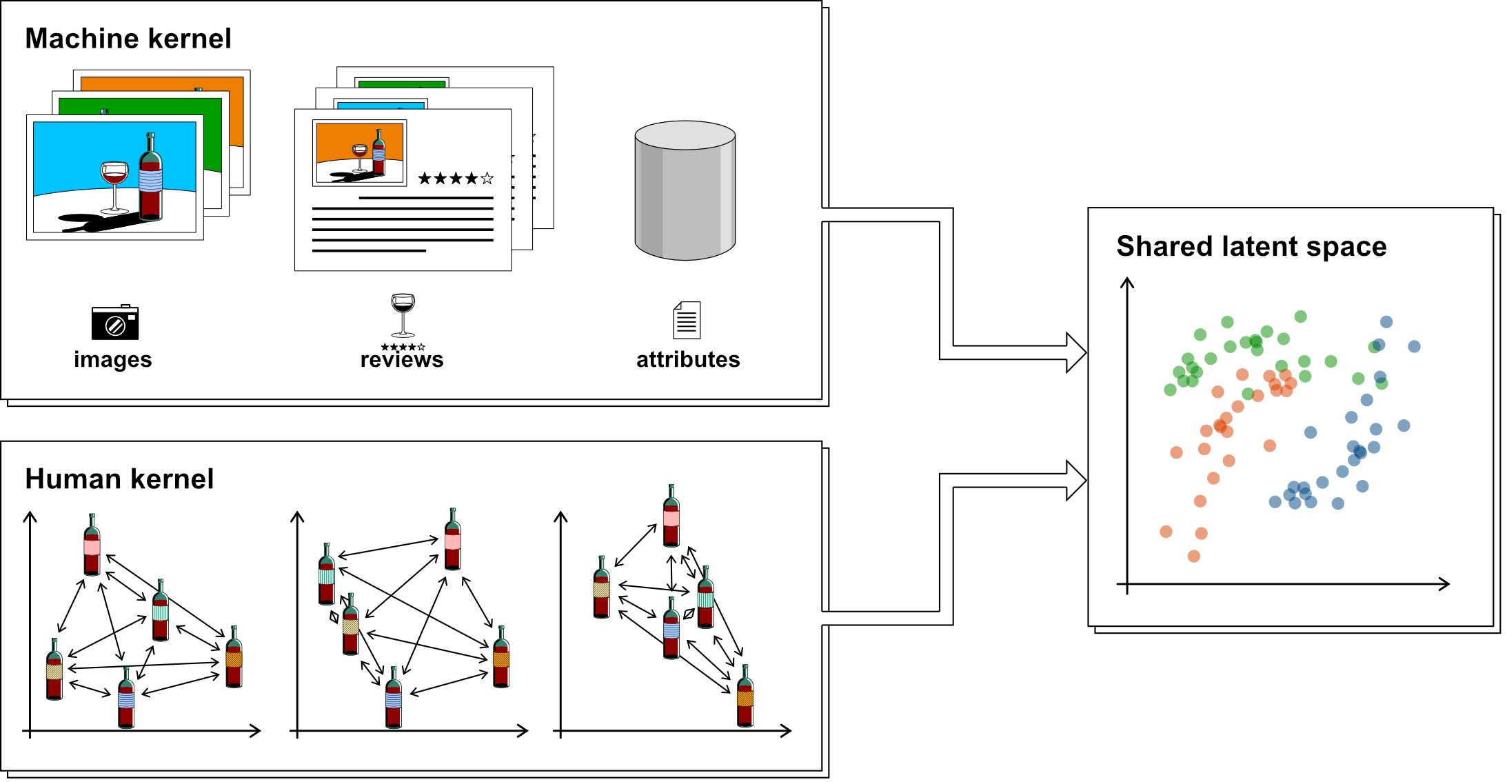
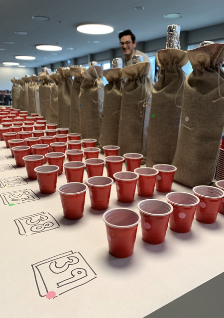
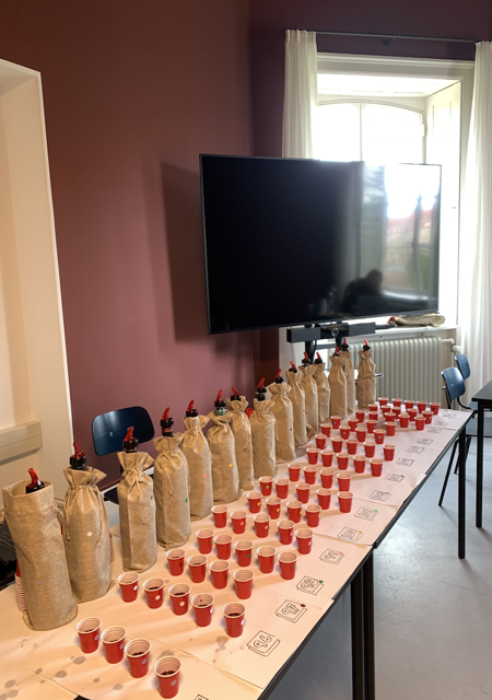
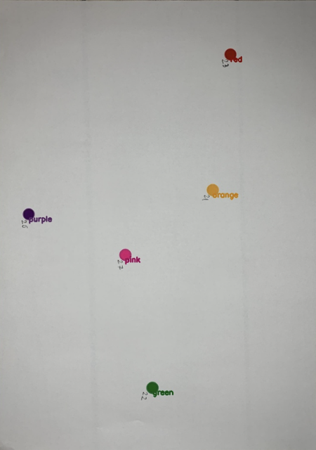
We organized a large sensory study to obtain human-annotated flavor profiles of the wines. The study applies the “Napping” methodology (Pagès, 2005), which is commonly used to conduct consumer surveys (Kim et al., 2013; Ribeiro et al., 2020). In this study, 256 participants annotated their perceived taste similarities of various wines. In Fig. 1, the “human kernel” illustrates how participants were instructed to place wines on a sheet of paper based on how similar they perceived their flavor to be. The Napping method enabled us to annotate wine flavors with a high level of detail and harness the perception of a broad spectrum of individuals. It scales well, as asking a participant to annotate five wines yields 10 pairwise annotations. All participants combined annotated more than 5k flavor distances.
To complement these annotations, we curate images of wine labels, user reviews, and wine attributes (country of origin, alcohol percentage, price, and grape composition) from the Vivino platform, a popular online social network for wine enthusiasts.111https://vivino.com WineSensed, therefore, represents a large, multimodal dataset that merges user-generated content with sensory assessments, bridging the gap between subjective consumer perception and objective flavor profiles.
Along with the dataset, we propose Flavor Embeddings from Annotated Similarity & Text-Image (FEAST) that leverages recent developments in large multimodal models to embed user reviews and images of wine labels into a low-dimensional, latent representation that contains semantic and structural information that correlates with taste. Our model aligns this representation with the flavor annotations from our user study. We find that this combined representation yields a “flavor space” that models coarse flavor concepts like alcohol percentage, country, grape, and the year of production, while also being aligned with more intricate human perception of flavor.
Experimentally, we find (1) that using the pairwise distances (rather than ordering) of the annotated wines improves the flavor representation, which confirms the established methodology in food science, and validates our annotation process. (2) We discover that using multiple data modalities (images, text, and flavor annotations) boosts the flavor representations, highlighting the usefulness of our multimodal dataset. (3) Finally, we show that the proposed multimodal model produces a flavor space with a high alignment with humans’ perception of flavor.
2 Background and related work
Multimodal representations. Learning a shared representation between modalities can reveal useful representations that generalize well and appear grounded in reality. Pioneering work (de Sa, 1994) proposes to learn the correlation between vision and audio. A number of deep learning methods propose to use large collections of weakly annotated data to learn shared vision-language representations (Joulin et al., 2016; Desai and Johnson, 2021; Radford et al., 2021b; Mahajan et al., 2018), shared audio-text representations (Agostinelli et al., 2023), shared vision-audio representations (Ngiam et al., 2011; Owens et al., 2016; Arandjelovic and Zisserman, 2017; Narasimhan et al., 2022; Hu et al., 2022), shared vision-touch (Yang et al., 2022) representations, or shared sound and Inertial Measurement Unit (IMU) representations (Chen et al., 2023). Recently, ImageBind (Girdhar et al., 2023) showed that images can bind multiple modalities (images, text, audio, depth, thermal, IMU) into a shared representation. While recent advances in other areas of multimodal learning have been fueled by large datasets, the difficulty of quantifying and collecting high-quality flavor data has made it challenging for the machine learning community to develop similar representations for flavor.
Quantifying flavor. Understanding and engineering flavor is a central part of food science and essential in the quest towards healthy and sustainable food production (Savage, 2012), but the use of machine learning methods to this end is still in its infancy. Fuentes et al. (2019) found a correlation between seasonal weather characteristics, and wine quality and aroma profiles, thereby verifying what wine producers have long held to be true. Similarly, Gupta (2018) found that sulfur dioxide, pH, and alcohol levels are useful for predicting wine quality. Due to the difficulty of gathering quality perception data, much work focuses on how ‘low-level’ chemical aspects related to ‘high-level’ taste properties, e.g. in assessing the quality of chocolate and beer (Gunaratne et al., 2019; Gonzalez Viejo et al., 2018).
Analyzing a person’s perception of wine is challenging due to the complex nature of flavor, which remains ill-understood, and the difficulty in obtaining consistent verbal descriptions of taste across individuals. Napping (Pagès, 2005) is the de facto method to analyze perceived taste in consumer surveys. Participants receive taste samples and are instructed to place them on a sheet of paper based on how similar they perceive their taste to be, with closer meaning more similar. Such experiments are usually conducted with 10-25 participants and less than 20 variants of a product (Giacalone et al., 2013; Pagès et al., 2010; Mayhew et al., 2016). In this study, we scale this data collection process to 256 participants and 108 unique bottlings of red wine, resulting in over 400 napping papers collected and more than 5k annotated flavor distances. In contrast to previous works (Giacalone et al., 2013; Pagès et al., 2010; Mayhew et al., 2016) our objective is to incorporate taste as one of the modalities that contribute to the shared representations for improved grounding of machine learning models.
Human kernel learning. Annotating flavor with Napping (Pagès, 2005) does not provide image-flavor or text-flavor correspondences but rather relative flavor similarities between sampled products. According to (Miller, 2019) humans are better at describing abstract concepts such as taste with contrastive questions, such as “does wine X taste more similar to wine Y or Z?” For this reason, the machine learning community has used contrastive questions in multiple settings, e.g., for understanding how humans perceive light reflection from surfaces by presenting annotators with image triplets depicting the Stanford Bunny with varying material properties (Agarwal et al., 2007), to produce a genre embedding of musical artists (Van Der Maaten and Weinberger, 2012), and for discovering underlying narratives in online discussions (Christensen et al., 2022). Most relevant to our work is SNaCK (Wilber et al., 2015), which presents annotators with image triplets depicting foods and asked which two of them taste more similar, to obtain flavor triplets. They proposed to combine this high-level human flavor understanding with low-level image statistics to learn food concepts, e.g., that even though guacamole and wasabi look similar, their taste is not. Having humans annotate image triplets of foods works well for coarse concepts, but does not encompass nuanced differences in taste. In this work, we focus on the much finer-grained taste difference found in wines. These nuances and the complex nature of wine tasting, which involves taste and smell, are not easily conveyed through text or images.
Flavor datasets. The machine learning community has produced numerous food datasets for classifying which meal is in an image (Bossard et al., 2014; Min et al., 2020), retrieving a recipe given an image (Salvador et al., 2017; Li et al., 2022), or predicting the origin of wines (Dua and Graff, 2017). While it is possible to extract coarse information about taste from such datasets (Wilber et al., 2015), they do not encompass higher resolution details of taste, such as the differences between a Cabernet Sauvignon and Pinot Noir.
Similarly, the food science community has developed many datasets for understanding and predicting food flavors, nutrient content, and chemistry. Flavornet (Arn and Acree, 1998), a dataset on human-perceived aroma compounds, explores partly how smells relate to perceived bitterness or fruitiness in a wine. However, its limitation is its lack of context linking these odors to specific wine varieties and its limited focus on flavor aspects. FoodDB (Harrington et al., 2019) offers comprehensive information on a wide variety of food, its nutrient contents, potential health effects, and macro and micro constituents. However, it lacks user-generated reviews and sensory data, which are crucial for understanding the subjective human perception of food and wine. The Wine Data Set (Dua and Graff, 2017) focuses on wines, but only contains wines originating from one region in Italy, limiting the dataset’s ability to capture the broader diversity of flavor profiles of wines from various regions worldwide. Furthermore, Dua and Graff (2017) solely incorporate the chemical compounds present in each wine, without annotations of flavors and information associating specific wines with each chemical compound. In contrast to previous work, we present a multimodal dataset that contains a large corpus of images and reviews, as well as human-annotated flavor similarities.
3 The WineSensed dataset
We present WineSensed, a large, multimodal wine dataset that combines human flavor annotations, images, and reviews. In this section, we provide an overview of the curation process for each of these modalities.
Annotated flavors. The flavor data consists of over 5k human-annotated pairwise similarities between 108 unique bottlings. Each annotated pair is annotated at least five times to reduce noise.
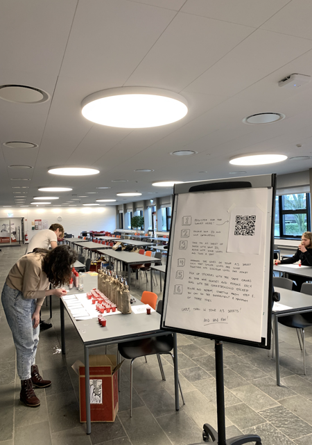
These annotations are collected through a series of wine-tasting events attended by a total of non-expert wine drinkers. Most participants were between 21-25 years old, and more than half of them were from Denmark. Each participant volunteered their time, dedicating a maximum of two hours to complete the annotations. The experiment was conducted in accordance with the ”De Videnskabsetiske Komiteer” (e. the Danish ethics committee for science) (see Appendix I).
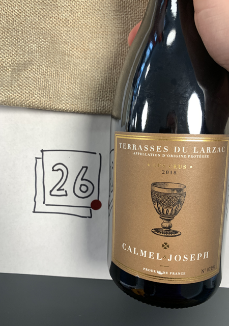
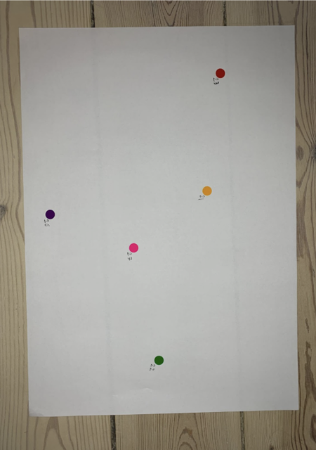
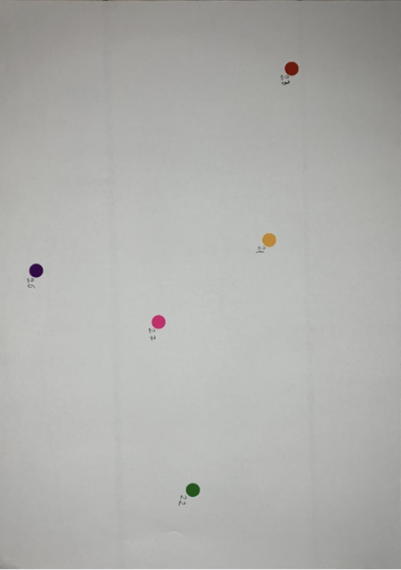
We randomly selected 5 wines for the participants to taste. The participants did not have access to any information regarding the individual wines. The wine was poured into non-transparent shot glasses and the labels of the wines were covered during the entire experiment. The participants were instructed to put colored stickers (representing each of the five wines) on a sheet of paper based on their taste similarity, closer meaning more similar. The participants could repeat the process up to three times, ensuring they did not consume more than 225 ml of wine. The average participant repeated the experiment two times.
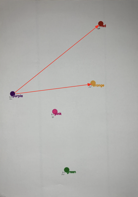
We automatically digitized the participants’ annotations by taking a photo of each filled-out sheet. We used the Harris corner detector (Harris et al., 1988) to find the corners of the paper and a homographic projection to obtain an aligned top-down view of the paper. The images were mapped into HSV color space and a threshold filter applied to find the different colored stickers that the participant used to represent the wines. Having identified the location, we computed the Euclidean pixel-wise distance between all pairs of points, resulting in a distance matrix of wine similarities. A more detailed description of the collection and digitization of the napping papers can be found in D.
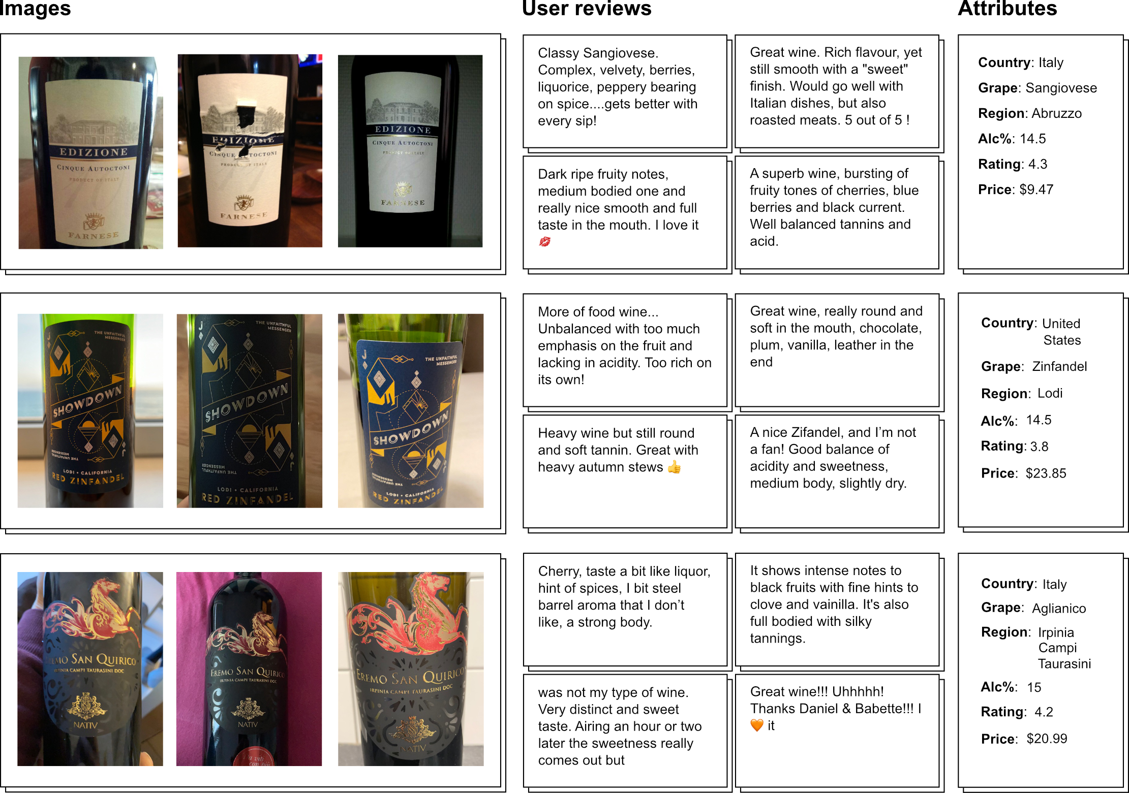
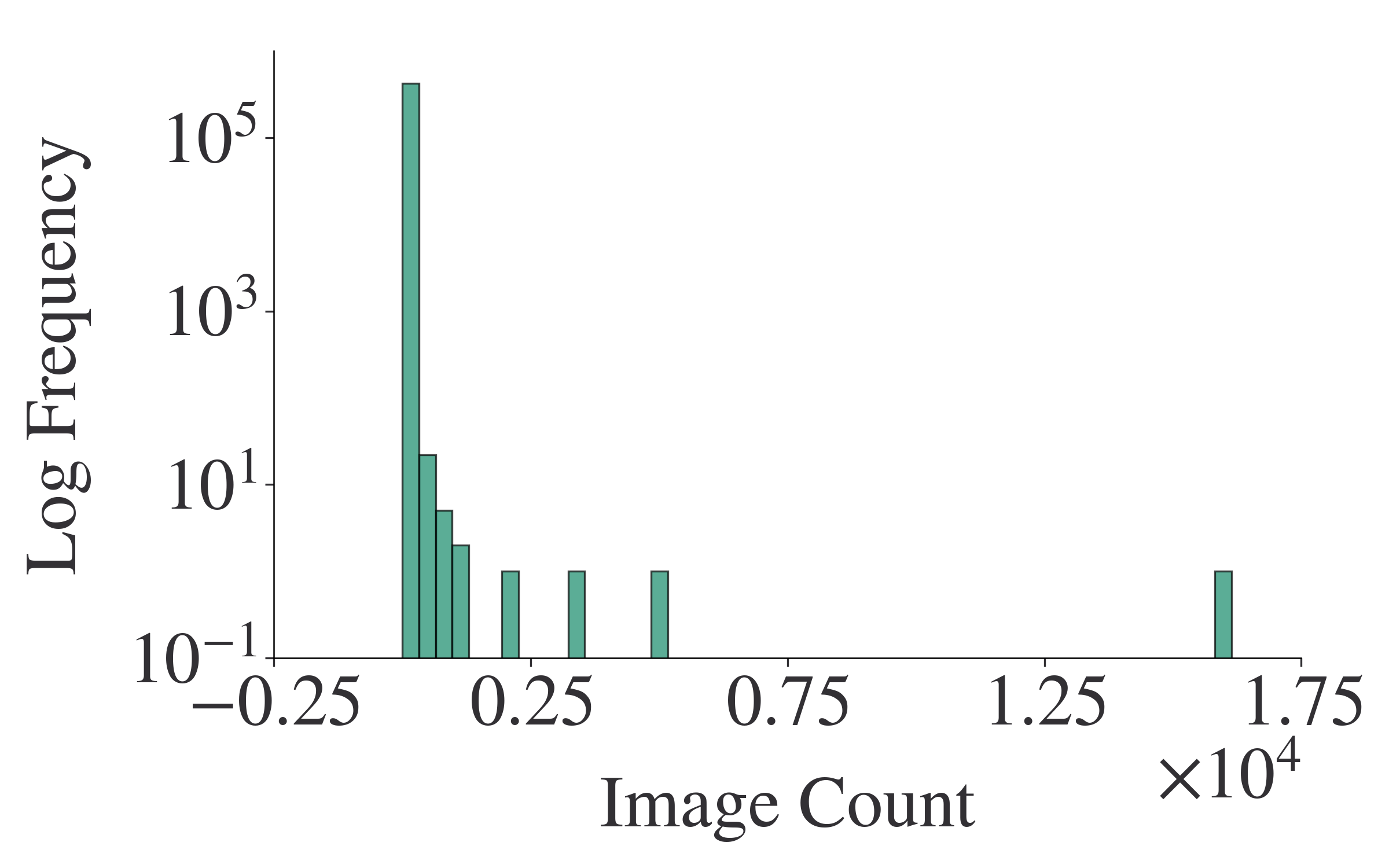
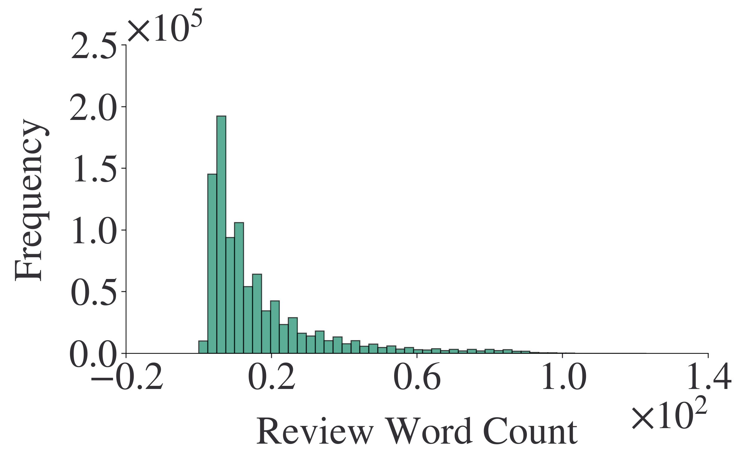
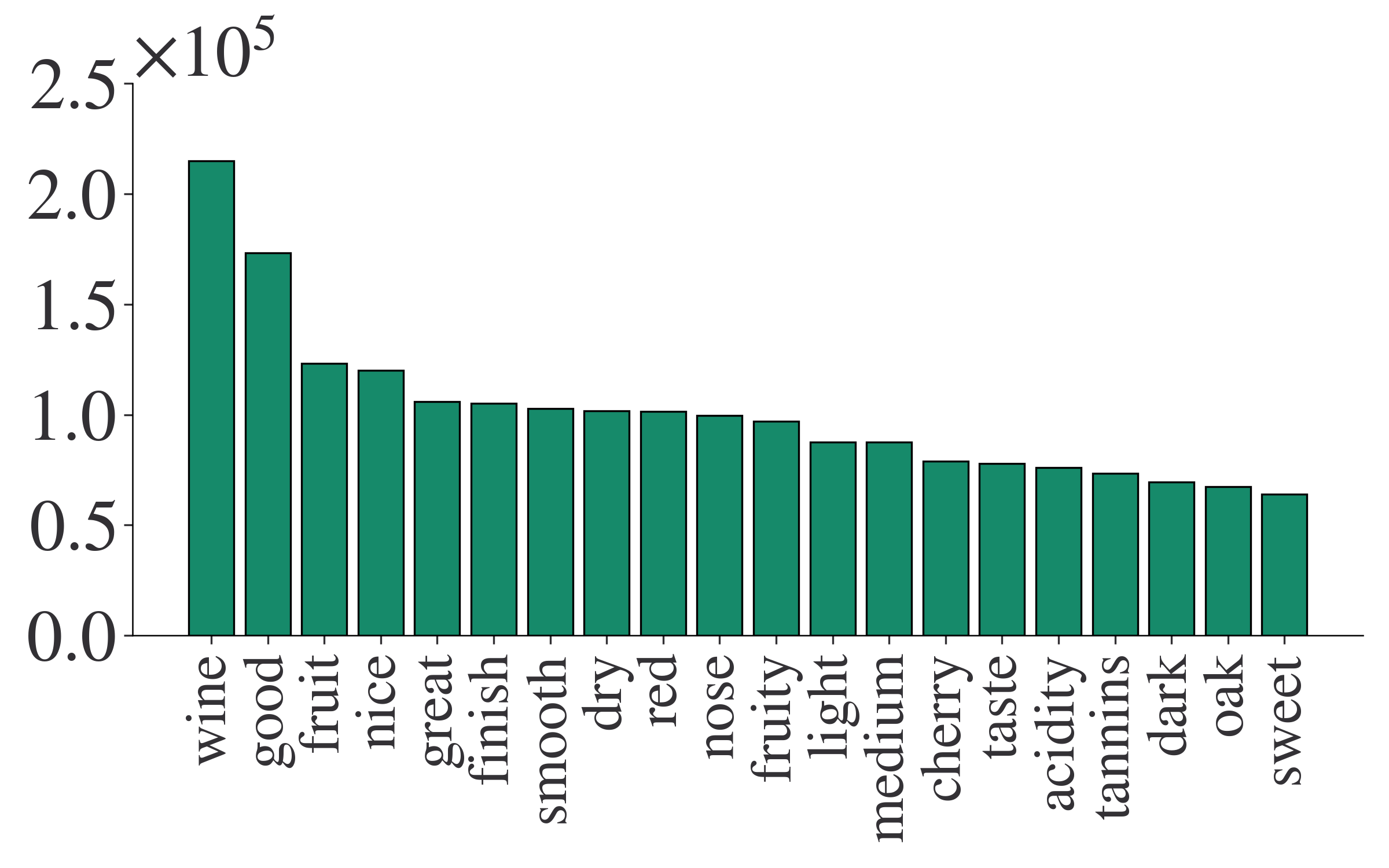
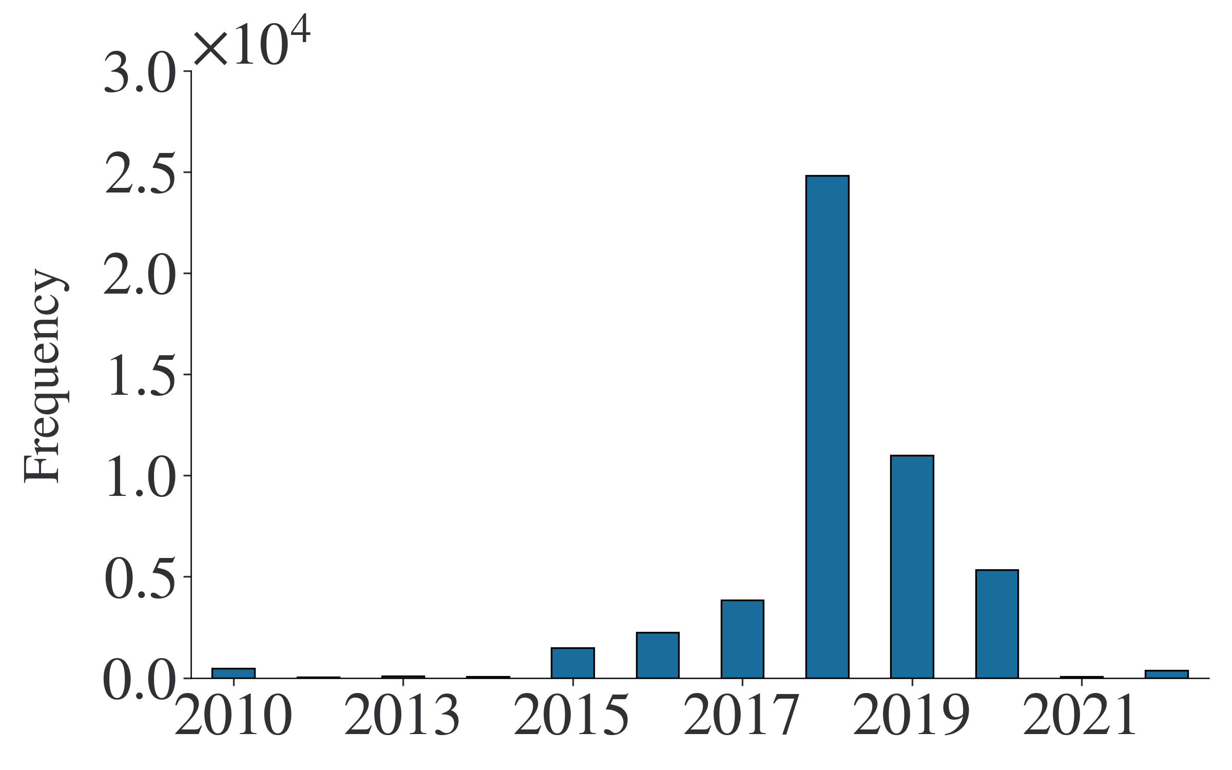
User-reviews. We curated 824k text reviews from the Vivino platform. The reviews were filtered to contain at least characters to avoid non-informative reviews such as ‘good’ and ‘bad.’ Fig. 2 shows examples of user-reviews. The reviews are free text and can contain special tokens such as emojis. The reviews tend to describe price, pairing, and general terms of wine. Some also describe which flavors the reviewer tastes. These reviews are subjective and can vary based on personal factors and context, leading to inconsistent flavor profiles. Moreover, they only contain coarse flavor descriptions and focus more on aspects like preference, price, occasion, and so forth. Fig. 4 shows the distribution of word count per review, number of reviews per unique bottling, and the most common keywords.
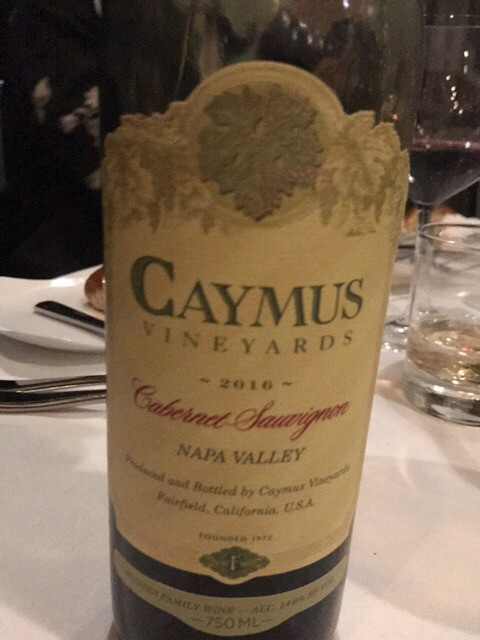
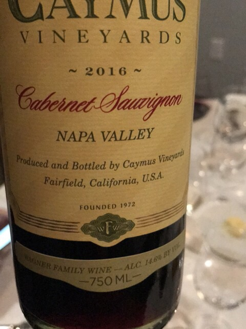
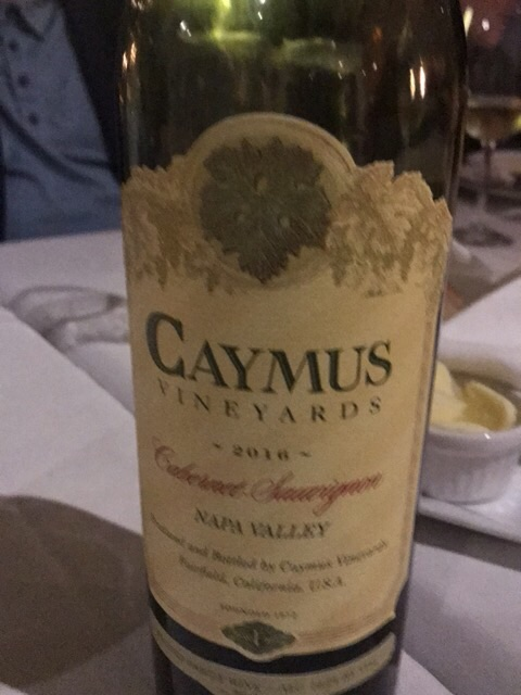
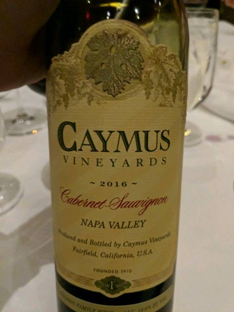
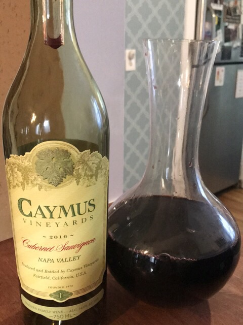
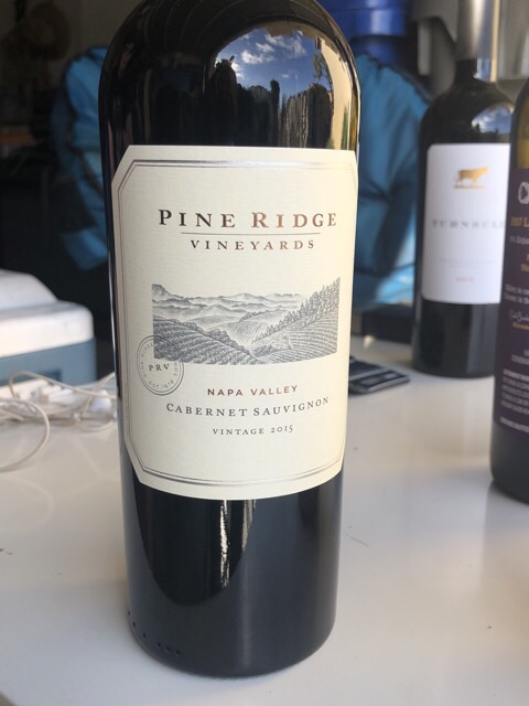
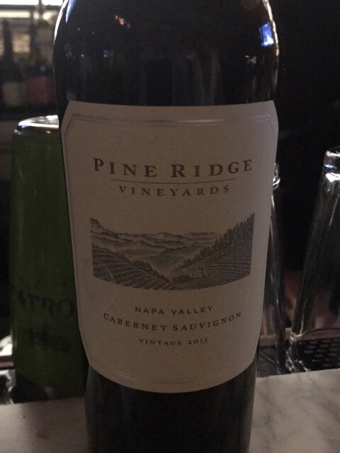
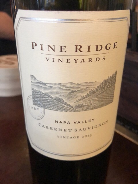
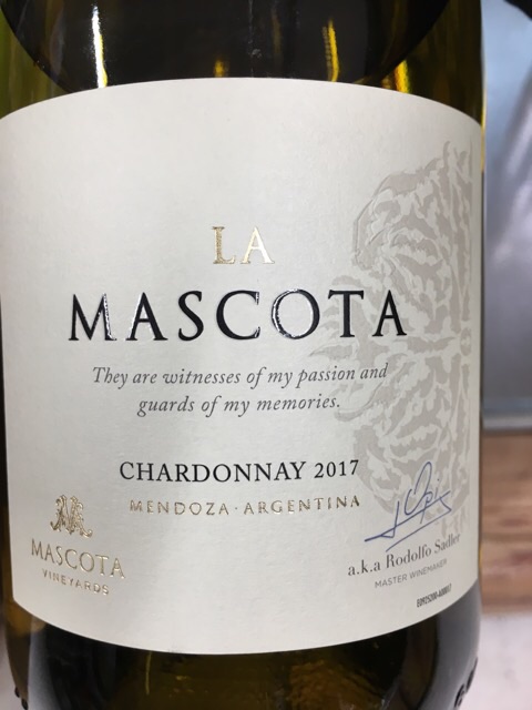
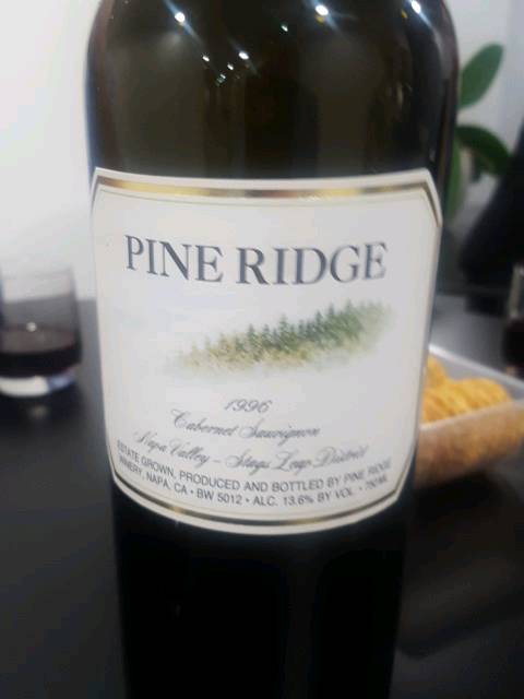
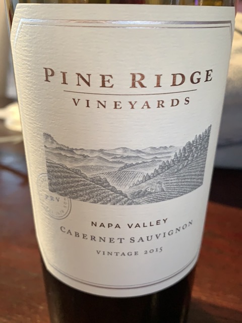
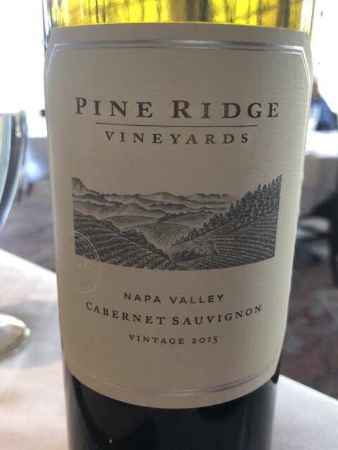
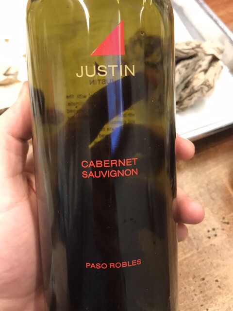
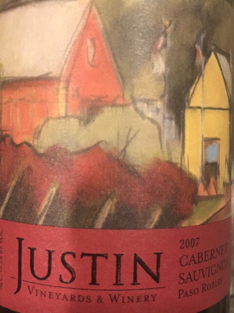
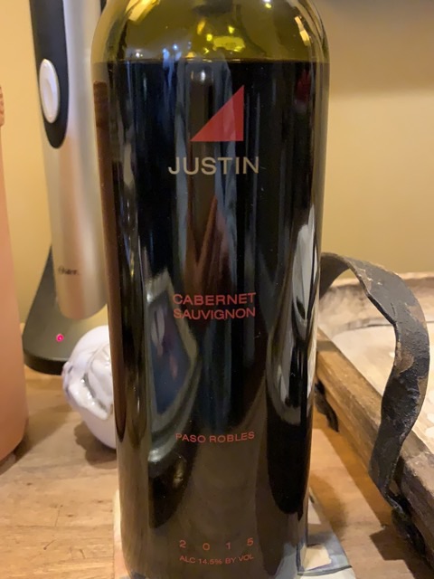
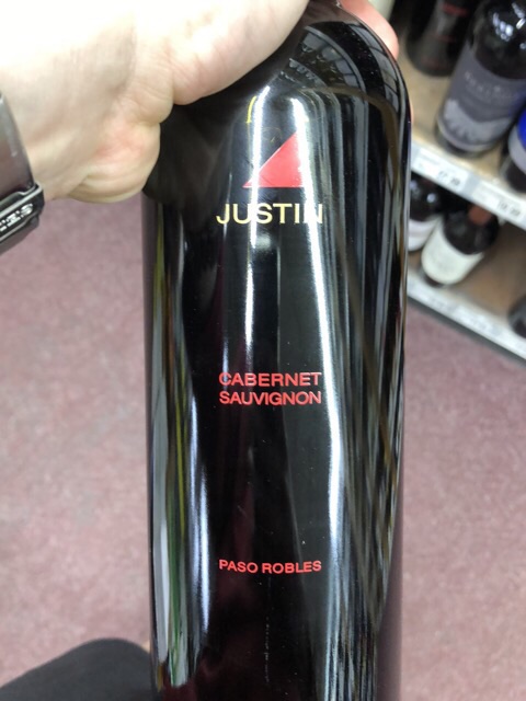
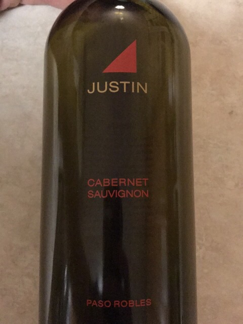
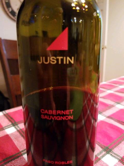
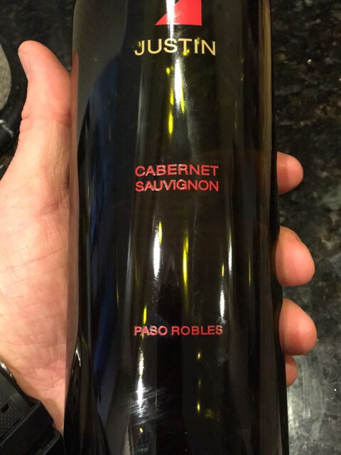
Images. The dataset has 897k images of wine labels. Wine labels are known to play a major role in a consumer’s decision to purchase a particular wine, so it is reasonable to believe that label design carries information regarding the taste of the wine (Talbot, 2019). Fig. 3 shows examples of images from the dataset. The images vary in their viewing angle, illumination, and image composition.
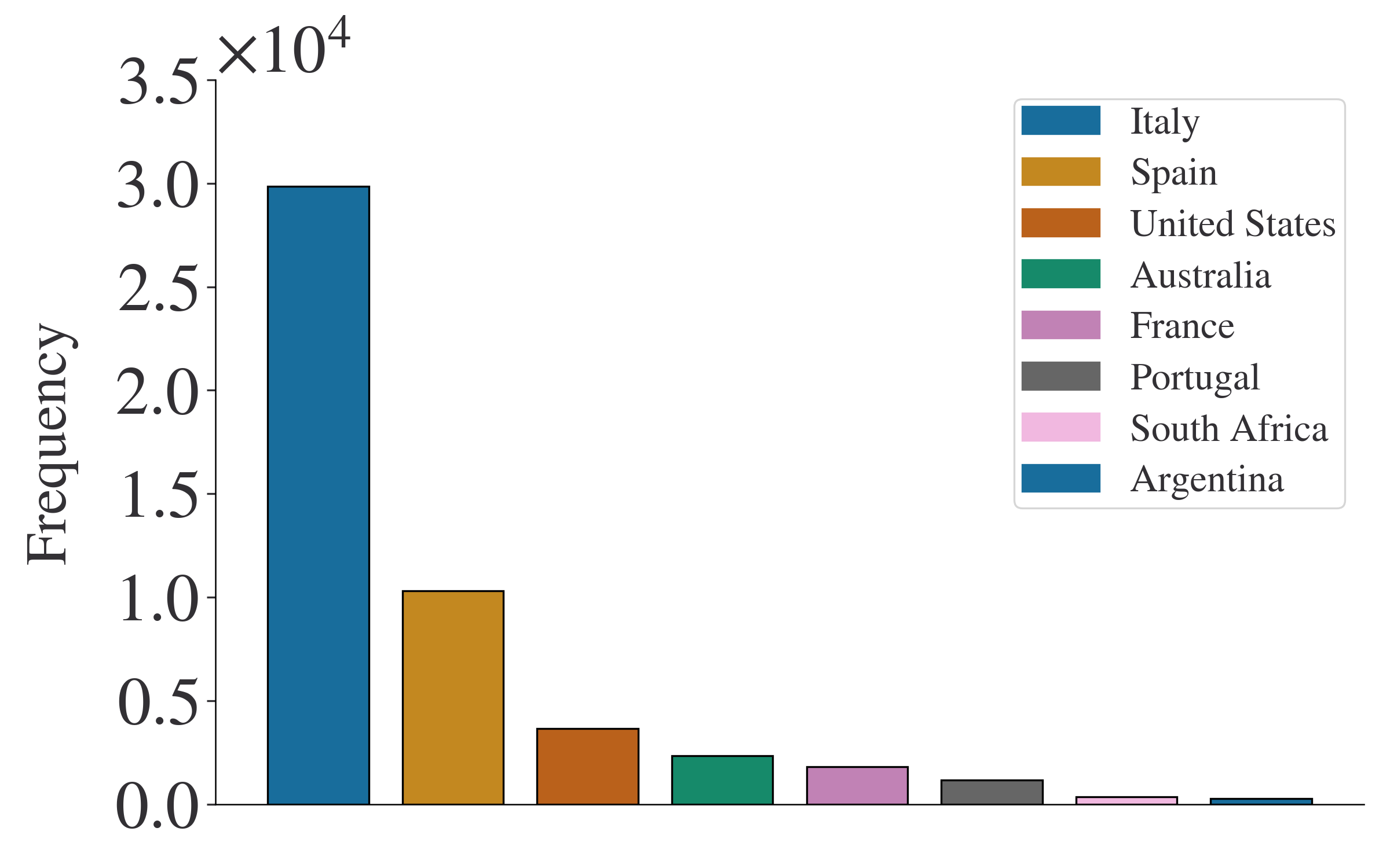
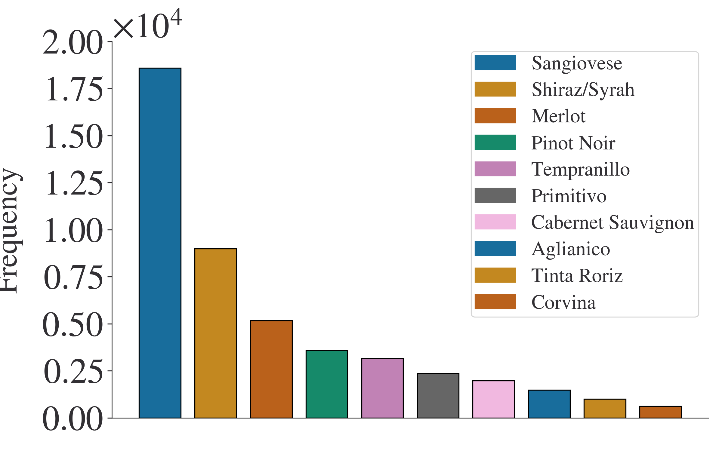
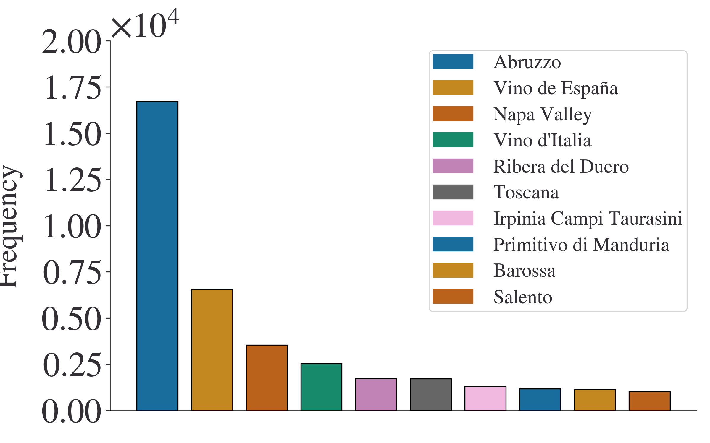
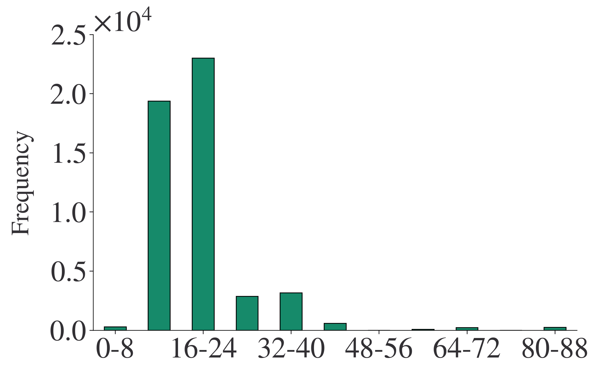
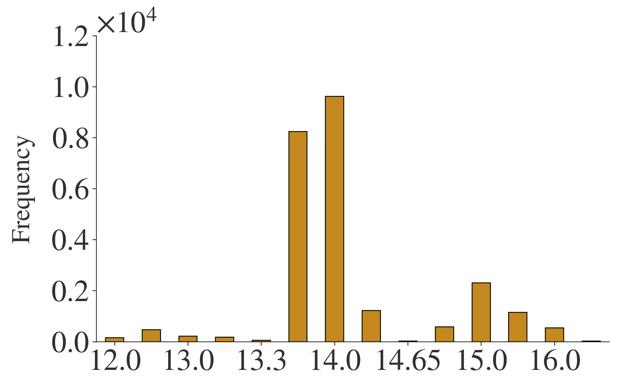
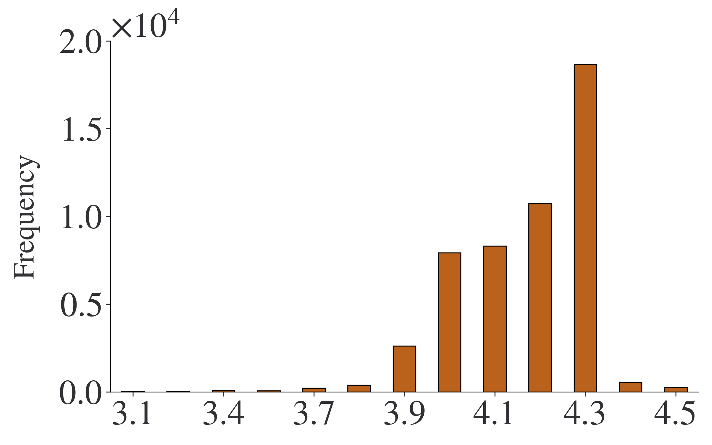
Attributes. Each wine is associated with the geographical location of the vineyard (both country and region), grape varietal composition, vintage, alcohol content, pricing, and average user rating. Fig. 5 shows the distribution of these attributes. Most wines originate from Italy, with Sangiovese being the most commonly used grape. The wines occupy the lower range of the price spectrum, with the most expensive ones priced at around 40 USD. The attributes are available for 5% of the dataset entries.
4 Flavor Embeddings from Annotated Similarity & Text-Image (FEAST)
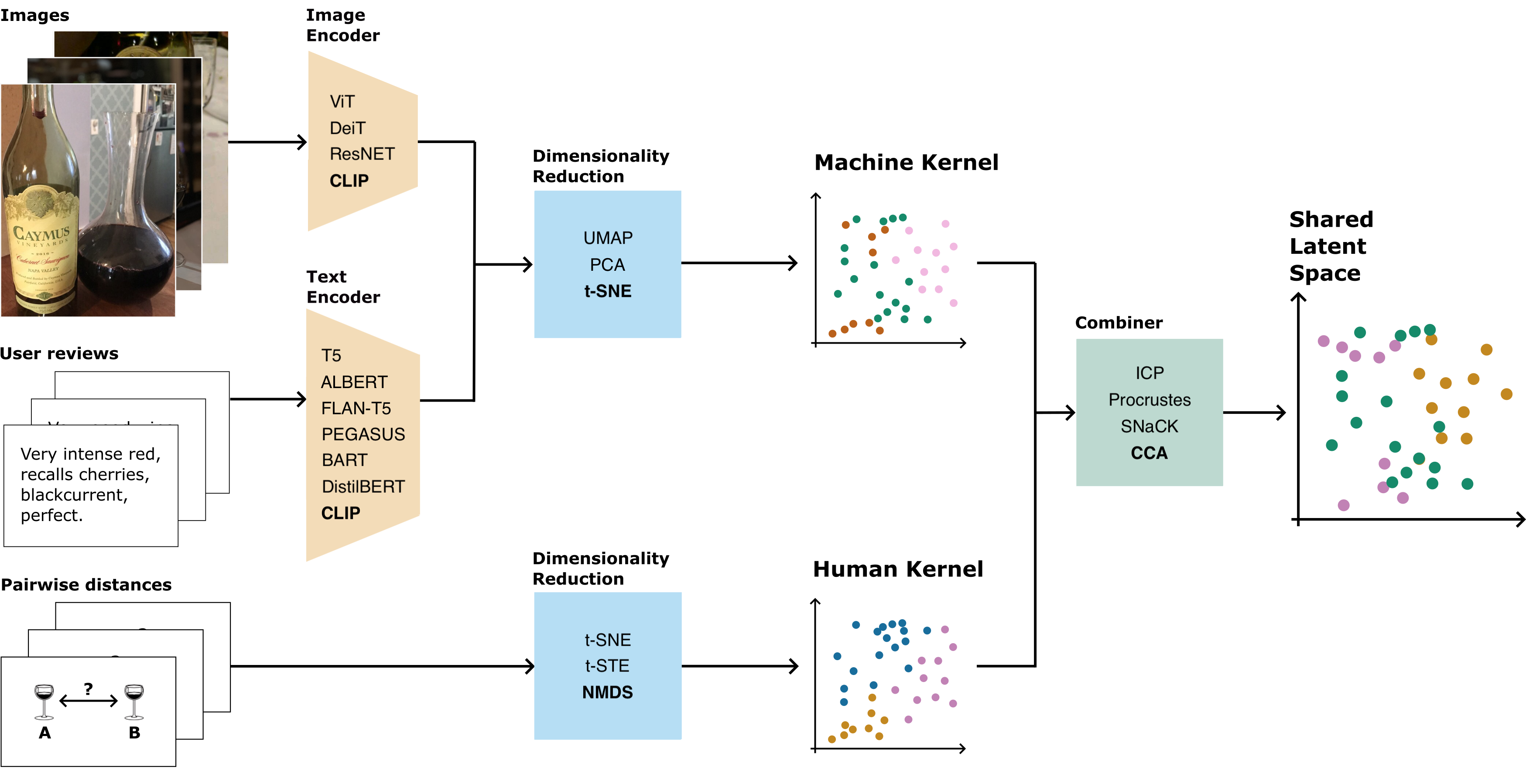
The embeddings of recent large image and text networks contain structural and semantic information, however, they do not model the intricacies of human flavor. We propose FEAST, a method to align these embeddings to the human perception of flavor using a small set of human-annotated flavor similarities. FEAST takes text and/or images as input, as well as human-annotated flavor similarities. It outputs a unified embedding that aligns with human sensory perception. Fig. 6 provides an overview of the proposed method.
We first embed the text and/or images into a latent space with CLIP (Radford et al., 2021a). We use CLIP because of its large training corpus and its image-text aligned latent space, however, highlights that other pretrained networks can be used. We use t-SNE (Van der Maaten and Hinton, 2008) to reduce the dimensionality of the latent space to 2, which simplifies and constrain the later alignment with the pairwise flavor annotations.
The pairwise distances are embedded into a 2D representation using Non-metric multidimensional scaling (NMDS) with the SMACOF strategy (de Leeuw and Mair, 2009). NMDS allows us to preserve the original flavor distances provided by humans in a shared space, where each unique bottling is represented with point location, rather than pairwise distances. MDS is commonly used in food science to analyze sensory annotations from Napping studies (Pineau et al., 2022; Varela and Ares, 2012; Nestrud and Lawless, 2010).
We then align these two 2D representations to get a joint representation that benefits from the structural and semantic information of the image and/or text representations, scales to unobserved unique bottlings, and is aligned with the human perception of flavor. We use Canonical Correlation Analysis (CCA) (Harold, 1936) to align the two representations. CCA identifies and connects common patterns between these representation spaces, ensuring that the final representation is consistent across all input modalities.
5 Experiments
We conduct two experiments on the WineSensed dataset. First, we explore how well recent large pretrained language and image models explain wine attributes that correlate with the flavor of a wine. Second, we explore multimodal models’ capabilities to represent more intricate flavors.
Experimental setup. We explore several configurations of human kernels, machine kernels, and “combiners” that align the two representations. Fig. 6 provides an overview of our baselines. The human kernel is formed with t-STE (Van Der Maaten and Weinberger, 2012), a low dimensional graph representation reduced with t-SNE or NMDS, where the notable difference is that t-STE discards the flavor distances, and solely optimizes for triplet orderings. The machine kernel consists of two steps: (1) we use a pretrained model to embed text and/or images into a low dimensional space, (2) which is then compressed into a two-dimensional space. For (1), we explore DistilBert (Sanh et al., 2019), T5 (Raffel et al., 2020), ALBERT (Lan et al., 2019), BART (Lewis et al., 2019), PEGASUS (Zhang et al., 2020), FLAN-T5 (Chung et al., 2022) and CLIP for embedding text and ViT (Dosovitskiy et al., 2020), ResNet (He et al., 2016), DeiT (Touvron et al., 2021), and CLIP for embedding images. For (2), we explore t-SNE, UMAP (McInnes et al., 2018), and PCA (Pearson, 1901). For the combiners, we experiment with CCA, Iterative Closest Point (ICP) (Chen and Medioni, 1992), Procrustes (Gower, 1975) and SNaCK. For a more detailed description of the implementation and software packages used, please refer to E the Appendix.
5.1 Coarse flavor predictions
We first explore how well pretrained language and vision models explain wine attributes that correlate with flavor. We then investigate if using FEAST to align the machine and human kernels improves the representation.
Implementation details. We use a balanced SVM classifier with an RBF kernel as well as a Multi-layer Perceptron neural network to predict wine attributes of the flavor embeddings. We predict price, alcohol percentage, rating, region, country, and grape variety as these attributes are known to correlate with the perceived wine flavor. We mitigate imbalanced class distributions with class weight balancing and oversampling of the minority classes. We report the accuracy averaged over the seven attributes computed through 5-fold cross-validation. The accuracy measures how coherent the embeddings are with the flavor attributes. A more detailed description of the implementation can be found in J.2.
| Acc | |||
|---|---|---|---|
| Machine kernel | Modality | SVM | NN |
| Random | 0.11 | 0.11 | |
| ViT | Image | 0.09 | 0.13 |
| DeiT | Image | 0.14 | 0.15 |
| ResNET | Image | 0.15 | 0.16 |
| CLIP | Image | 0.11 | 0.15 |
| T5 | Text | 0.15 | 0.16 |
| ALBERT | Text | 0.15 | 0.18 |
| BART | Text | 0.16 | 0.15 |
| DistilBERT | Text | 0.15 | 0.17 |
| CLIP | Text | 0.16 | 0.18 |
| FLAN-T5 | Text | 0.15 | 0.17 |
| PEGASUS | Text | 0.13 | 0.13 |
| BART | Text | 0.11 | 0.15 |
| Acc | ||
|---|---|---|
| Modality | SVM | NN |
| Flavor | 0.16 | 0.11 |
| Image | 0.11 | 0.15 |
| Text | 0.16 | 0.18 |
| Text+Flavor | 0.23 | 0.18 |
| Image+Text | 0.22 | 0.25 |
| Image+Flavor | 0.23 | 0.18 |
| Image+Text+Flavor | 0.28 | 0.26 |
| Reducer | Acc | |
|---|---|---|
| Human Kernel | SVM | NN |
| Random | 0.11 | 0.11 |
| t-STE | 0.13 | 0.10 |
| t-SNE | 0.15 | 0.13 |
| NMDS | 0.16 | 0.13 |
| Reducer | Acc | |
|---|---|---|
| Machine Kernel | SVM | NN |
| UMAP | 0.15 | 0.18 |
| PCA | 0.20 | 0.21 |
| t-SNE | 0.22 | 0.25 |
| Acc | ||
|---|---|---|
| Combiner | SVM | NN |
| ICP | 0.21 | 0.24 |
| Procrustes | 0.19 | 0.23 |
| SNaCK | 0.23 | 0.24 |
| CCA | 0.28 | 0.26 |
Results. Tables 3, 3 and 3 ablates our proposed method and summarizes our main conclusions. Please see Section J.2 for per attribute classification accuracy for all combinations of machine kernels, human kernels, modalities, reduces, and combiners.
Table 3 shows that most pretrained image and text models yield slightly higher performance than the random baseline. The text encoders are slightly better than the image encoders. BART and CLIP perform the best. All encoders in the table use t-SNE to reduce the embedding to 2D. Table 3 (middle) shows t-SNE yields better accuracy than UMAP and PCA when using a CLIP encoder.
Table 3 (top) shows that NMDS performs better than t-STE. NMDS uses the relative distances between annotations, whereas t-STE discretizes the annotations and considers only the ordering within each triplet. The results suggest that the pairwise distances are useful to model the flavor space. Table 3 (bottom) shows that using CCA to align the two representations yields higher accuracy than SNaCK or ICP.
Table 3 shows that including flavor as a modality increases the accuracy, e.g. using flavor to align the image or text embeddings lead to higher accuracy. Using CLIP followed by t-SNE, NMDS, and CCA to combine language, vision, and flavor into a single representation leads to the best configurations, illustrating that the human annotations are useful for learning a flavor representation. Maybe most surprisingly, we show that each modality by itself is on par with the random baseline, but their combination produces a latent space that much better describes the flavor attributes.
5.2 Fine-grained flavor predictions
We now proceed to evaluate more intricate flavor predictions by using human-annotated flavor similarities as ground truth.
Implementation details. To evaluate our representation, we measure the Triplet Agreement Ratio (TAR) (van der Maaten and Weinberger, 2012) between our predicted flavor embeddings and the human-annotated flavors. TAR measures the agreement between a triplet derived from the latent space and the ground truth triplets from the flavor annotations. Higher TAR means that the ordering of distances in the latent space corresponds to the human perception of flavor. This measure indicates how aligned the two representations are, and provides a higher granularity of flavor prediction than flavor attributes. A more detailed description of the implementation can be found in F.
Results. Table 4 ablates FEAST and shows that for the higher granularity predictions both the pretrained text and image encoders improve upon the random baseline. We show that including the human kernel with NMDS further improves the TAR scores. This highlights the usefulness of the flavor distances recorded by the human annotators. In Appendix F, we show results from all configurations of human kernels, machine kernels, reducers, and combiners. We find that NMDS consistently yields better performance than t-STE, and that combining human and machine kernels improves the TAR scores across multiple model configurations.
| Machine Kernel | Human Kernel | Combiner | Modality | TAR |
|---|---|---|---|---|
| Random | 0.5 | |||
| CLIP + t-SNE | Text | 0.82 | ||
| CLIP + t-SNE | Image | 0.82 | ||
| CLIP + t-SNE | Image + Text | 0.81 | ||
| CLIP + t-SNE | Image + Flavor | 0.89 | ||
| CLIP + t-SNE | Text + Flavor | 0.88 | ||
| CLIP + t-SNE | NMDS | CCA | Image + Text + Flavor | 0.91 |
6 Discussion & Conclusion
In this paper, we introduce WineSensed, an extensive multimodal dataset curated for flavor modeling. The dataset comprises over 897k images and 824k reviews, and has over 5k human-annotated pairwise flavor similarities, obtained via a sensory study involving 256 participants. We propose a simple algorithm, FEAST, to align semantic information from machine kernels with flavor similarities from human annotators in a shared flavor representation. We find that combining these modalities improves both coarse and fine-grained flavor predictions.
WineSensed further strengthens the collaboration between the food science and machine learning communities, introduces flavor as a modality in multimodal models, and serves as an entry point for the development of machine learning models for flavor analysis and potentially deepening our comprehension of wine flavors. The dataset and the proposed procedures open many interesting possibilities, such as using flavor to ground foundation models or extending the dataset with other modalities, such as chemical composition, or other food categories.
Constraints and considerations. The dataset serves as a novel first step to including human-annotated flavor in the array of modalities in multimodal models. Its current scope is constrained to a selected group of red wines, predominantly Italian ones. While this enables a more nuanced understanding of flavors within Italian wines, it may not represent the broader spectrum of red wines globally. Furthermore, the dataset’s emphasis on wines prevalent in Western cultures highlights a geo-cultural bias. Expanding the dataset to encompass more diverse drink types from different cultures could provide a more comprehensive understanding of global flavor perception. Lastly, the Napping methodology is not immune to the influences of participants’ backgrounds and experiences. Individual perceptions, shaped by personal histories, can introduce nuances in the data. Though leveraging non-expert wine drinkers for flavor annotations introduces subjectivity, this approach, inspired by common sensory study practices, broadens taste perspectives, enhances study accessibility, and offers commercial value, with multiple annotations per entry mitigating individual biases. Exploring a broader range of foods and beverages remains a valuable direction for future work.
Acknowlegements. This work was supported by the Pioneer Centre for AI, DNRF grant number P1, and by research grant (42062) from VILLUM FONDEN. This project received funding from the European Research Council (ERC) under the European Union’s Horizon 2020 research and innovation programme (grant agreement 757360), as well as the Danish Data Science Academy (DDSA).
References
- [1] ftfy: Fixes Text for You. https://pypi.org/project/ftfy/. Accessed: 2023-06-10.
- [2] h5py: Pythonic interface to the HDF5 binary data format. https://www.h5py.org/. Accessed: 2023-06-10.
- [3] Hugging Face – The AI community building the future. https://huggingface.co/. Accessed: 2023-06-10.
- [4] ICP: Iterative Closest Point Implementation in Python. https://github.com/richardos/icp. Accessed: 2023-06-10.
- [5] imbalanced-learn: Tackling the Curse of Imbalanced Datasets in Python. https://imbalanced-learn.org/stable/. Accessed: 2023-06-10.
- [6] Matplotlib: Python plotting library. https://matplotlib.org/. Accessed: 2023-06-10.
- [7] Natural Language Toolkit. https://www.nltk.org/. Accessed: 2023-06-10.
- [8] open-clip-torch: OpenAI CLIP Implementation in PyTorch. https://pypi.org/project/open-clip-torch/. Accessed: 2023-06-10.
- [9] pandas: Powerful Data Structures for Data Analysis, Time Series, and Statistics. https://pandas.pydata.org/. Accessed: 2023-06-10.
- [10] psutil: Cross-platform lib for process and system monitoring in Python. https://pypi.org/project/psutil/. Accessed: 2023-06-10.
- [11] scikit-learn: Machine Learning in Python. https://scikit-learn.org/. Accessed: 2023-06-10.
- [12] seaborn: Statistical data visualization. https://seaborn.pydata.org/. Accessed: 2023-06-10.
- [13] Searching for Structure in Unfalsifiable Claims. https://github.com/captainE/Searching-for-Structure-in-Unfalsifiable-Claims. Accessed: 2023-06-10.
- [14] torchmetrics: The Metrics Library for PyTorch. https://torchmetrics.readthedocs.io/en/latest/. Accessed: 2023-06-10.
- [15] transformers: State-of-the-Art Natural Language Processing. https://huggingface.co/transformers/. Accessed: 2023-06-10.
- [16] t-Distributed Stochastic Triplet Embedding Implementation in Theano. https://github.com/gcr/tste-theano/blob/master/tste.py. Accessed: 2023-06-10.
- [17] Uniform Manifold Approximation and Projection. https://umap-learn.readthedocs.io/en/latest/. Accessed: 2023-06-10.
- [18] urllib3: HTTP library with thread-safe connection pooling, file post, and more. https://pypi.org/project/urllib3/. Accessed: 2023-06-10.
- Agarwal et al. [2007] Sameer Agarwal, Josh Wills, Lawrence Cayton, Gert Lanckriet, David Kriegman, and Serge Belongie. Generalized non-metric multidimensional scaling. In Artificial Intelligence and Statistics, pages 11–18. PMLR, 2007.
- Agostinelli et al. [2023] Andrea Agostinelli, Timo I Denk, Zalán Borsos, Jesse Engel, Mauro Verzetti, Antoine Caillon, Qingqing Huang, Aren Jansen, Adam Roberts, Marco Tagliasacchi, et al. Musiclm: Generating music from text. arXiv preprint arXiv:2301.11325, 2023.
- Arandjelovic and Zisserman [2017] Relja Arandjelovic and Andrew Zisserman. Look, listen and learn. In Proceedings of the IEEE international conference on computer vision, pages 609–617, 2017.
- Arn and Acree [1998] H Arn and TE Acree. Flavornet: A database of aroma compounds based on odor potency in natural products. Developments in food science, 40:27–28, 1998.
- Bossard et al. [2014] Lukas Bossard, Matthieu Guillaumin, and Luc Van Gool. Food-101–mining discriminative components with random forests. In Computer Vision–ECCV 2014: 13th European Conference, Zurich, Switzerland, September 6-12, 2014, Proceedings, Part VI 13, pages 446–461. Springer, 2014.
- Chen and Medioni [1992] Yang Chen and Gérard Medioni. Object modelling by registration of multiple range images. Image and vision computing, 10(3):145–155, 1992.
- Chen et al. [2023] Ziyang Chen, Shengyi Qian, and Andrew Owens. Sound localization from motion: Jointly learning sound direction and camera rotation. arXiv, 2023.
- Christensen et al. [2022] Peter Ebert Christensen, Frederik Warburg, Menglin Jia, and Serge Belongie. Searching for structure in unfalsifiable claims. arXiv preprint arXiv:2209.00495, 2022.
- Chung et al. [2022] Hyung Won Chung, Le Hou, Shayne Longpre, Barret Zoph, Yi Tay, William Fedus, Eric Li, Xuezhi Wang, Mostafa Dehghani, Siddhartha Brahma, et al. Scaling instruction-finetuned language models. arXiv preprint arXiv:2210.11416, 2022.
- de Leeuw and Mair [2009] Jan de Leeuw and Patrick Mair. Multidimensional scaling using majorization: Smacof in r. Journal of Statistical Software, 31(3):1–30, 2009. doi: 10.18637/jss.v031.i03. URL https://www.jstatsoft.org/index.php/jss/article/view/v031i03.
- de Sa [1994] Virginia R de Sa. Learning classification with unlabeled data. Advances in neural information processing systems, pages 112–112, 1994.
- Desai and Johnson [2021] Karan Desai and Justin Johnson. Virtex: Learning visual representations from textual annotations. In Proceedings of the IEEE/CVF conference on computer vision and pattern recognition, pages 11162–11173, 2021.
- Dosovitskiy et al. [2020] Alexey Dosovitskiy, Lucas Beyer, Alexander Kolesnikov, Dirk Weissenborn, Xiaohua Zhai, Thomas Unterthiner, Mostafa Dehghani, Matthias Minderer, Georg Heigold, Sylvain Gelly, et al. An image is worth 16x16 words: Transformers for image recognition at scale. arXiv preprint arXiv:2010.11929, 2020.
- Dua and Graff [2017] Dheeru Dua and Casey Graff. UCI machine learning repository, 2017. URL http://archive.ics.uci.edu/ml.
- Fuentes et al. [2019] Sigfredo Fuentes, Eden Tongson, Damir D Torrico, and Claudia Gonzalez Viejo. Modeling pinot noir aroma profiles based on weather and water management information using machine learning algorithms: A vertical vintage analysis using artificial intelligence. Foods, 9(1):33, 2019.
- Giacalone et al. [2013] Davide Giacalone, Leticia Machado Ribeiro, and Michael Bom Frøst. Consumer-based product profiling: Application of partial napping® for sensory characterization of specialty beers by novices and experts. Journal of Food Products Marketing, 19(3):201–218, 2013.
- Girdhar et al. [2023] Rohit Girdhar, Alaaeldin El-Nouby, Zhuang Liu, Mannat Singh, Kalyan Vasudev Alwala, Armand Joulin, and Ishan Misra. Imagebind: One embedding space to bind them all. arXiv preprint arXiv:2305.05665, 2023.
- Gonzalez Viejo et al. [2018] Claudia Gonzalez Viejo, Sigfredo Fuentes, Damir Torrico, Kate Howell, and Frank R Dunshea. Assessment of beer quality based on foamability and chemical composition using computer vision algorithms, near infrared spectroscopy and machine learning algorithms. Journal of the Science of Food and Agriculture, 98(2):618–627, 2018.
- Gower [1975] John C Gower. Generalized procrustes analysis. Psychometrika, 40:33–51, 1975.
- Grover and Leskovec [2016] Aditya Grover and Jure Leskovec. node2vec: Scalable feature learning for networks. In Proceedings of the 22nd ACM SIGKDD international conference on Knowledge discovery and data mining, pages 855–864, 2016.
- Gunaratne et al. [2019] Thejani M Gunaratne, Claudia Gonzalez Viejo, Nadeesha M Gunaratne, Damir D Torrico, Frank R Dunshea, and Sigfredo Fuentes. Chocolate quality assessment based on chemical fingerprinting using near infra-red and machine learning modeling. Foods, 8(10):426, 2019.
- Gupta [2018] Yogesh Gupta. Selection of important features and predicting wine quality using machine learning techniques. Procedia Computer Science, 125:305–312, 2018.
- Harold [1936] Hotelling Harold. Relations between two sets of variates. Biometrika, 28(3/4):321, 1936.
- Harrington et al. [2019] Richard Andrew Harrington, Vyas Adhikari, Mike Rayner, and Peter Scarborough. Nutrient composition databases in the age of big data: fooddb, a comprehensive, real-time database infrastructure. BMJ open, 9(6):e026652, 2019.
- Harris et al. [1988] Chris Harris, Mike Stephens, et al. A combined corner and edge detector. In Alvey vision conference, volume 15, pages 10–5244. Citeseer, 1988.
- He et al. [2016] Kaiming He, Xiangyu Zhang, Shaoqing Ren, and Jian Sun. Deep residual learning for image recognition. In Proceedings of the IEEE conference on computer vision and pattern recognition, pages 770–778, 2016.
- Hu et al. [2022] Xixi Hu, Ziyang Chen, and Andrew Owens. Mix and localize: Localizing sound sources in mixtures. Computer Vision and Pattern Recognition (CVPR), 2022.
- Joulin et al. [2016] Armand Joulin, Laurens Van Der Maaten, Allan Jabri, and Nicolas Vasilache. Learning visual features from large weakly supervised data. In Computer Vision–ECCV 2016: 14th European Conference, Amsterdam, The Netherlands, October 11–14, 2016, Proceedings, Part VII 14, pages 67–84. Springer, 2016.
- Kim et al. [2013] Young-Kyung Kim, Laureen Jombart, Dominique Valentin, and Kwang-Ok Kim. A cross-cultural study using napping®: Do korean and french consumers perceive various green tea products differently? Food Research International, 53(1):534–542, 2013.
- Lan et al. [2019] Zhenzhong Lan, Mingda Chen, Sebastian Goodman, Kevin Gimpel, Piyush Sharma, and Radu Soricut. Albert: A lite bert for self-supervised learning of language representations. arXiv preprint arXiv:1909.11942, 2019.
- Lewis et al. [2019] Mike Lewis, Yinhan Liu, Naman Goyal, Marjan Ghazvininejad, Abdelrahman Mohamed, Omer Levy, Ves Stoyanov, and Luke Zettlemoyer. Bart: Denoising sequence-to-sequence pre-training for natural language generation, translation, and comprehension. arXiv preprint arXiv:1910.13461, 2019.
- Li et al. [2022] Ming Li, Lin Li, Qing Xie, Jingling Yuan, and Xiaohui Tao. Mealrec: A meal recommendation dataset. arXiv preprint arXiv:2205.12133, 2022.
- Mahajan et al. [2018] Dhruv Mahajan, Ross Girshick, Vignesh Ramanathan, Kaiming He, Manohar Paluri, Yixuan Li, Ashwin Bharambe, and Laurens Van Der Maaten. Exploring the limits of weakly supervised pretraining. In Proceedings of the European conference on computer vision (ECCV), pages 181–196, 2018.
- Mayhew et al. [2016] Emily Mayhew, Shelly Schmidt, and Soo-Yeun Lee. Napping-ultra flash profile as a tool for category identification and subsequent model system formulation of caramel corn products. Journal of food science, 81(7):S1782–S1790, 2016.
- McInnes et al. [2018] Leland McInnes, John Healy, and James Melville. Umap: Uniform manifold approximation and projection for dimension reduction. arXiv preprint arXiv:1802.03426, 2018.
- Miller [2019] Tim Miller. Explanation in artificial intelligence: Insights from the social sciences. Artificial intelligence, 267:1–38, 2019.
- Min et al. [2020] Weiqing Min, Linhu Liu, Zhiling Wang, Zhengdong Luo, Xiaoming Wei, Xiaolin Wei, and Shuqiang Jiang. Isia food-500: A dataset for large-scale food recognition via stacked global-local attention network. In Proceedings of the 28th ACM International Conference on Multimedia, pages 393–401, 2020.
- Narasimhan et al. [2022] Medhini Narasimhan, Shiry Ginosar, Andrew Owens, Alexei A Efros, and Trevor Darrell. Strumming to the beat: Audio-conditioned contrastive video textures. In Proceedings of the IEEE/CVF Winter Conference on Applications of Computer Vision, pages 3761–3770, 2022.
- Nestrud and Lawless [2010] Michael A Nestrud and Harry T Lawless. Perceptual mapping of apples and cheeses using projective mapping and sorting. Journal of Sensory Studies, 25(3):390–405, 2010.
- Ngiam et al. [2011] Jiquan Ngiam, Aditya Khosla, Mingyu Kim, Juhan Nam, Honglak Lee, and Andrew Y Ng. Multimodal deep learning. In Proceedings of the 28th international conference on machine learning (ICML-11), pages 689–696, 2011.
- Owens et al. [2016] Andrew Owens, Phillip Isola, Josh McDermott, Antonio Torralba, Edward H Adelson, and William T Freeman. Visually indicated sounds. In Proceedings of the IEEE conference on computer vision and pattern recognition, pages 2405–2413, 2016.
- Pagès [2005] Jérôme Pagès. Collection and analysis of perceived product inter-distances using multiple factor analysis: Application to the study of 10 white wines from the loire valley. Food quality and preference, 16(7):642–649, 2005.
- Pagès et al. [2010] Jérome Pagès, Marine Cadoret, and Sébastien Lê. The sorted napping: A new holistic approach in sensory evaluation. Journal of Sensory Studies, 25(5):637–658, 2010.
- Pearson [1901] Karl Pearson. Liii. on lines and planes of closest fit to systems of points in space. The London, Edinburgh, and Dublin philosophical magazine and journal of science, 2(11):559–572, 1901.
- Pineau et al. [2022] Nicolas Pineau, Alicia Girardi, Céline Lacoste Gregorutti, Laurence Fillion, and David Labbe. Comparison of rata, cata, sorting and napping® as rapid alternatives to sensory profiling in a food industry environment. Food Research International, 158:111467, 2022.
- Radford et al. [2021a] Alec Radford, Jong Wook Kim, Chris Hallacy, Aditya Ramesh, Gabriel Goh, Sandhini Agarwal, Girish Sastry, Amanda Askell, Pamela Mishkin, Jack Clark, Gretchen Krueger, and Ilya Sutskever. Learning transferable visual models from natural language supervision. CoRR, abs/2103.00020, 2021a. URL https://arxiv.org/abs/2103.00020.
- Radford et al. [2021b] Alec Radford, Jong Wook Kim, Chris Hallacy, Aditya Ramesh, Gabriel Goh, Sandhini Agarwal, Girish Sastry, Amanda Askell, Pamela Mishkin, Jack Clark, et al. Learning transferable visual models from natural language supervision. In International conference on machine learning, pages 8748–8763. PMLR, 2021b.
- Raffel et al. [2020] Colin Raffel, Noam Shazeer, Adam Roberts, Katherine Lee, Sharan Narang, Michael Matena, Yanqi Zhou, Wei Li, and Peter J Liu. Exploring the limits of transfer learning with a unified text-to-text transformer. The Journal of Machine Learning Research, 21(1):5485–5551, 2020.
- Ribeiro et al. [2020] Michele Nayara Ribeiro, Daniela Maria Rodrigues, Renata Abadia Reis Rocha, Letícia Rodrigues Silveira, João Paulo Ferreira Condino, Arlindo Curzi Júnior, Vanessa Rios de Souza, Cleiton Antônio Nunes, and Ana Carla Marques Pinheiro. Optimising a stevia mix by mixture design and napping: A case study with high protein plain yoghurt. International Dairy Journal, 110:104802, 2020.
- Salvador et al. [2017] Amaia Salvador, Nicholas Hynes, Yusuf Aytar, Javier Marin, Ferda Ofli, Ingmar Weber, and Antonio Torralba. Learning cross-modal embeddings for cooking recipes and food images. In Proceedings of the IEEE conference on computer vision and pattern recognition, pages 3020–3028, 2017.
- Sanh et al. [2019] Victor Sanh, Lysandre Debut, Julien Chaumond, and Thomas Wolf. Distilbert, a distilled version of bert: Smaller, faster, cheaper and lighter. arxiv 2019. arXiv preprint arXiv:1910.01108, 2019.
- Savage [2012] Neil Savage. Technology: The taste of things to come. Nature, 486(7403):S18–S19, 2012.
- Talbot [2019] Paul Talbot. Why wine label design matters so much. Forbes, 2019.
- Touvron et al. [2021] Hugo Touvron, Matthieu Cord, Matthijs Douze, Francisco Massa, Alexandre Sablayrolles, and Hervé Jégou. Training data-efficient image transformers & distillation through attention. In International conference on machine learning, pages 10347–10357. PMLR, 2021.
- Van der Maaten and Hinton [2008] Laurens Van der Maaten and Geoffrey Hinton. Visualizing data using t-sne. Journal of machine learning research, 9(11), 2008.
- van der Maaten and Weinberger [2012] Laurens van der Maaten and Kilian Weinberger. Stochastic triplet embedding. In 2012 IEEE International Workshop on Machine Learning for Signal Processing, pages 1–6, 2012. doi: 10.1109/MLSP.2012.6349720.
- Van Der Maaten and Weinberger [2012] Laurens Van Der Maaten and Kilian Weinberger. Stochastic triplet embedding. In 2012 IEEE International Workshop on Machine Learning for Signal Processing, pages 1–6. IEEE, 2012.
- Varela and Ares [2012] Paula Varela and Gastón Ares. Sensory profiling, the blurred line between sensory and consumer science. a review of novel methods for product characterization. Food Research International, 48(2):893–908, 2012.
- Virtanen et al. [2020] Pauli Virtanen, Ralf Gommers, Travis E. Oliphant, Matt Haberland, Tyler Reddy, David Cournapeau, Evgeni Burovski, Pearu Peterson, Warren Weckesser, Jonathan Bright, Stéfan J. van der Walt, Matthew Brett, Joshua Wilson, K. Jarrod Millman, Nikolay Mayorov, Andrew R. J. Nelson, Eric Jones, Robert Kern, Eric Larson, C J Carey, İlhan Polat, Yu Feng, Eric W. Moore, Jake VanderPlas, Denis Laxalde, Josef Perktold, Robert Cimrman, Ian Henriksen, E. A. Quintero, Charles R. Harris, Anne M. Archibald, Antônio H. Ribeiro, Fabian Pedregosa, Paul van Mulbregt, and SciPy 1.0 Contributors. SciPy 1.0: Fundamental Algorithms for Scientific Computing in Python. Nature Methods, 17:261–272, 2020. doi: 10.1038/s41592-019-0686-2.
- Wilber et al. [2015] Michael Wilber, Iljung S Kwak, David Kriegman, and Serge Belongie. Learning concept embeddings with combined human-machine expertise. In Proceedings of the IEEE International Conference on Computer Vision, pages 981–989, 2015.
- Yang et al. [2022] Fengyu Yang, Chenyang Ma, Jiacheng Zhang, Jing Zhu, Wenzhen Yuan, and Andrew Owens. Touch and go: Learning from human-collected vision and touch. Neural Information Processing Systems (NeurIPS) - Datasets and Benchmarks Track, 2022.
- Zhang et al. [2020] Jingqing Zhang, Yao Zhao, Mohammad Saleh, and Peter Liu. Pegasus: Pre-training with extracted gap-sentences for abstractive summarization. In International Conference on Machine Learning, pages 11328–11339. PMLR, 2020.
Appendix A Project webpage
We provide a project webpage for the dataset that can be found here: https://thoranna.github.io/learning_to_taste/, which contains a link to the dataset and the code to reproduce our experiments. Additionally, we provide more examples from our dataset and images from the data collection.
Appendix B License
The WineSensed dataset is licensed under the Creative Commons Attribution-NonCommercial-NoDerivatives 4.0 International License. Details can be found here: https://creativecommons.org/licenses/by-nc-nd/4.0/.
Appendix C The WineSensed file structure
Our dataset is currently available here: https://data.dtu.dk/articles/dataset/WineSensed_Learning_to_Taste_A_Multimodal_Wine_Dataset/23376560. The dataset will be maintained on this site, which is hosted on a server run by the Technical University of Denmark.
WineSensed contains a metadata.zip file consisting of the files participants.csv, which contains information connecting participants to annotations in the experiment, images_reviews_attributes.csv, which contains reviews, links to images, and wine attributes, and napping.csv, which contains the coordinates of each wine on the napping paper, alongside information connecting each coordinate pair to the wines being annotated and the participant that annotated them. The chunk_<chunk num>.zip folders contain the images of the wines in the dataset in .jpg format.
napping.csv contains the following fields:
-
•
session_round_name: session number during the event_name, at most three sessions per event (maps to experiment_round in participants.csv)
-
•
event_name: name of the data collection event (maps to the same attribute in participants.csv)
-
•
experiment_no: the serial number of the napping paper in the session_round_name in which it was collected (maps to experiment_no in participants.csv)
-
•
experiment_id: id of the wine annotated
-
•
coor1: x-axis coordinate on the napping paper
-
•
coor2: y-axis coordinate on the napping paper
-
•
color: color of the sticker used
participants.csv contains the following fields:
-
•
session_round_name: session number during the event_name, at most three sessions per event (maps to experiment_round in napping.csv)
-
•
event_name: name of data-collection event (maps to event_name in napping.csv)
-
•
experiment_no: the serial number of the napping paper in the session_round_name in which it was collected (maps to experiment_no in napping.csv)
-
•
round_id: round number (from 1-3)
-
•
participant_id: id the participant was given in the experiment
images_reviews_attributes.csv contains the following fields:
-
•
vintage_id: vintage id of the wine
-
•
image: image link (each <image name>.jpg in chunk_<chunk num>.zip can be mapped to a corresponding image link in this column by removing the /p prefix from the link).
-
•
review: user review of the wine
-
•
experiment_id: id the wine got during data collection (each experiment_id can be mapped to the same column in napping.csv)
-
•
year: year the wine was produced
-
•
winery_id: id of the winery that produced the wine
-
•
wine: name of the wine
-
•
alcohol: the wine’s alcohol percentage
-
•
country: the country where the wine was produced
-
•
region: the region where the wine was produced
-
•
price: price of the wine in USD (collected 05/2023)
-
•
rating: average rating of the wine (collected 05/2023)
-
•
grape: the wine’s grape composition, represented as a comma-separated list ordered in descending sequence of the percentage contribution of each grape variety to the overall blend.
Appendix D Data collection details
The annotations in WineSensed were collected through a series of wine-tasting events attended by a total of 256 non-expert wine drinkers. Most participants were between 21-25 years old, and more than half of them were from Denmark. The experiment was conducted in accordance with the ”De Videnskabsetiske Komiteer” (e. the Danish ethics committee for science).
Five wines were selected at random for the participants to taste. The participants did not have access to any information regarding the individual wines. The wine was poured into non-transparent shot glasses and the labels of the wines were covered during the entire experiment. The participants were instructed to put colored stickers (representing each of the five wines) on a sheet of paper based on their taste similarity, closer meaning more similar. The participants could repeat the process up to three times, ensuring they did not consume more than 225 ml of wine. The average participant repeated the experiment two times. Figure 7 provides a visual representation of the data collection events.
The participants’ annotations were automatically digitized by taking a photo of each filled-out sheet. We used the Harris corner detector to find the corners of the paper and a homographic projection to obtain an aligned top-down view of the paper. The images were mapped into HSV color space and a threshold filter applied to find the different colored stickers that the participant used to represent the wines. Having identified the location, we computed the Euclidean pixel-wise distance between all pairs of points, resulting in a distance matrix of wine similarities. Figure 8 provides a visual representation of the procedure used to process the napping papers.
Appendix E Implementation details for flavor space generation
Preprocessing. For the image data, we resized images to a 256x256 pixel format, applied a central crop to bring the images down to 224x224 pixels. Subsequently, we converted them into a tensor format, followed by normalization using mean and standard deviation values for each color channel (RGB).
For the user reviews, we first converted the text to lowercase to maintain consistency. Then, we removed punctuation marks to minimize noise. We further eliminated stopwords using the nltk library’s English stopword list since these words usually do not contribute significantly to the overall meaning of the reviews. After these preprocessing steps, the data was tokenized and reassembled into a clean text string.
The preprocessing of human-annotated data varied based on its intended use, either as a distance matrix, triplets or graph. In the first case, we calculated the Euclidean distances between each data point and arranged these distances into an matrix, where is the total number of annotated wines. The matrix element had a value of if there were no annotated distances between wines and . For triplets, we constructed a list of triplets derived from the computed Euclidean distances. We generated triplets based on the Euclidean distances, such that is closer to than to ; i.e. . In order to make a graph representation, we used the euclidean distance matrix to form a graph where the similarities between wines form the weights on the edges and the nodes represent the wines.
Dimensionality reduction. In our experiments, we used several dimensionality reduction methods such as NMDS, t-STE, t-SNE, PCA, and UMAP. For these methods, we prepared two embedding pipelines, one to reduce the dimensionality of machine kernel, and another to reduce the dimensionality of the human kernel.
For the human kernel, NMDS, t-STE, t-SNE and node2vec [Grover and Leskovec, 2016] were used, depending on the form of the input data. The NMDS method was optimized through a series of hyperparameter tunings, including number of initial positions (n_inits), maximum number of iterations (max_iters), and tolerance to stress convergence (eps_values). These hyperparameters were evaluated using a range of values with the number of initial positions set to 5, 7, 10, the maximum number of iterations set to 300, 400, 500, 600, and the tolerance for stress convergence set to 1e-3, 1e-4, 1e-5.
The optimal hyperparameters for NMDS were selected by applying 5-fold cross validation (cross_val_score) using a K-nearest neighbors classifier model (KNeighborsClassifier) and oversampling to handle class imbalances in the data. In NMDS, The parameter metric was set to False to handle dissimilarities missing values represented by zeroes, and dissimilarity to precomputed as the input data was a distance matrix. Classification improvements during grid-search were not significant.
For the machine kernel pipeline, t-SNE, PCA, and UMAP, were used with a set seed to ensure the results’ reproducibility. These methods were called using their default hyperparameters in the respective libraries (see External packages).
Pre-trained models. The machine kernel embeddings were obtained using a collection of pre-trained text, image, and combined image-text models. All models were obtained from the HuggingFace [hug, ] library. The chosen models for the text were T5 (60.5M params), ALBERT (11.8M params), BART (406MM params), DistilBERT (67M params), FLAN-T5 (60M params), PEGASUS (568M params) and CLIP text model. For images, we chose ViT, DeiT, ResNET-50 and the CLIP image encoder. Lastly, we used CLIP for the combined image-text model. All embeddings were obtained from the models’ last hidden state.
Combiners. We leveraged four methods to combine the human kernel and the machine kernel: CCA, ICP, Procrustes and SNaCK. These three methods were employed using their default hyperparameters in their respective libraries (see External packages). In the case of CCA, Procrustes and ICP, we found common experiment identifiers across the two datasets and used them to align corresponding data points from the two datasets. Once the matrices were aligned, we subsequently applied CCA, Procrustes and ICP, respectively, and generated the combined embeddings.
SNaCK follows a slightly different process as it uses triplets from the human kernel and an embedding matrix from the machine kernel. We passed the triplet list (human kernel) and scaled embeddings (machine kernel) into SNaCK, which output the combined embedding.
External packages. We used several external packages: scikit-learn (v1.2.2) [sci, ], for dimensionality reduction, hyperparameter optimization, classification and human-and machine kernel combination; umap-learn (v0.5.3) [uma, ], for dimensionality reduction of the machine kernel; imblearn (v0.10.1) [imb, ], to address the problem of imbalanced datasets; snack sna , an implementation of SNaCK for human-and machine kernel combination; icp [icp, ], implementing the Iterative Closest Point algorithm for human-and machine kernel combination; tste [tst, ], an implementation of the t-Distributed Stochastic Triplet Embedding algorithm for the dimensionality reduction of human-kernel triplets; node2vec [Grover and Leskovec, 2016] for dimensionality reduction of the human kernel in graph form and procrustes [Virtanen et al., 2020], an implementation of the Procrustes algorithm for combining the human and machine kernel. Additionally, our project employed these Python packages: torchmetrics (v0.11.4) tor , ftfy (v6.1.1) [ftf, ], open-clip-torch (v2.19.0) [ope, ], transformers (v4.28.1) tra , pandas (v2.0.1) [pan, ], nltk (v3.8.1) [nlt, ], psutil (v5.9.5) [psu, ], urllib3 (v1.26.15) [url, ], matplotlib (v3.5.1) mat , seaborn (v0.11.2) [sea, ], and h5py (v3.8.0) [h5p, ].
Appendix F Details for fine-grained flavor predictions
Implementation details. The combination of dimensionality reduction methods, pre-trained models, and combiners described in F were used to generate multiple flavor spaces (using images, text and flavor). Additionally, to compare TAR across modalities, embeddings were produced for all combinations of modalities (text, image and flavor) using the relevant methods from F.
The human kernel was split into a training and a testing set. We made sure that for any given triplet in the testing set, none of the wines , or were present in the training set. The training set was processed and combined with the machine kernel using the reduction methods and combiners from F. The triplet agreement ratio was calculated using the level of agreement between the testing set and the triplets in the embeddings, by dividing agreements with disagreements. The triplet agreement ratio’s random baseline was set at 0.5, because when comparing triplets, either (i, j, k) or (j, i, k) could be chosen, which makes the ratio 0.5/1.0, similar to a random guess.
| Machine Kernel | Human Kernel | Combiner | Modality | TAR |
|---|---|---|---|---|
| DistilBeRT + UMAP | Text only | 0.81 | ||
| DistilBeRT + t-SNE | Text only | 0.81 | ||
| DistilBeRT + UMAP | MDS | CCA | Text + flavor | 0.91 |
| DistilBeRT + t-SNE | MDS | ICP | Text + flavor | 0.90 |
| DistilBeRT + t-SNE | MDS | CCA | Text + flavor | 0.90 |
| DistilBeRT + UMAP | t-STE | CCA | Text + flavor | 0.76 |
| DistilBeRT + t-SNE | t-STE | ICP | Text + flavor | 0.78 |
| DistilBeRT + t-SNE | t-STE | SNaCK | Text + flavor | 0.75 |
| T5 + UMAP | Text only | 0.82 | ||
| T5 + t-SNE | Text only | 0.82 | ||
| T5 + UMAP | MDS | CCA | Text + flavor | 0.89 |
| T5 + t-SNE | MDS | ICP | Text + flavor | 0.90 |
| T5 + t-SNE | MDS | CCA | Text + flavor | 0.90 |
| T5 + UMAP | t-STE | CCA | Text + flavor | 0.83 |
| T5 + t-SNE | t-STE | ICP | Text + flavor | 0.78 |
| T5 + t-SNE | t-STE | SNaCK | Text + flavor | 0.84 |
| ALBERT + UMAP | Text only | 0.80 | ||
| ALBERT + t-SNE | Text only | 0.81 | ||
| ALBERT + UMAP | MDS | CCA | Text + flavor | 0.89 |
| ALBERT + t-SNE | MDS | ICP | Text + flavor | 0.90 |
| ALBERT + t-SNE | MDS | CCA | Text + flavor | 0.90 |
| ALBERT + UMAP | t-STE | CCA | Text + flavor | 0.74 |
| ALBERT + t-SNE | t-STE | ICP | Text + flavor | 0.78 |
| ALBERT + t-SNE | t-STE | SNaCK | Text + flavor | 0.78 |
| BART + UMAP | Text only | 0.81 | ||
| BART + t-SNE | Text only | 0.82 | ||
| BART + UMAP | MDS | CCA | Text + flavor | 0.89 |
| BART + t-SNE | MDS | ICP | Text + flavor | 0.90 |
| BART + t-SNE | MDS | CCA | Text + flavor | 0.89 |
| BART + UMAP | t-STE | CCA | Text + flavor | 0.78 |
| BART + t-SNE | t-STE | ICP | Text + flavor | 0.79 |
| BART + t-SNE | t-STE | SNaCK | Text + flavor | 0.72 |
| Machine Kernel | Human Kernel | Combiner | Modality | TAR |
|---|---|---|---|---|
| ViT + UMAP | Image only | 0.83 | ||
| ViT + t-SNE | Image only | 0.82 | ||
| ViT + UMAP | MDS | CCA | Image + flavor | 0.90 |
| ViT + t-SNE | MDS | ICP | Image + flavor | 0.90 |
| ViT + t-SNE | MDS | CCA | Image + flavor | 0.90 |
| ViT + UMAP | t-STE | CCA | Image + flavor | 0.82 |
| ViT + t-SNE | t-STE | ICP | Image + flavor | 0.78 |
| ViT + t-SNE | t-STE | SNaCK | Image + flavor | 0.75 |
| ResNET + UMAP | Image only | 0.82 | ||
| ResNET + t-SNE | Image only | 0.82 | ||
| ResNET + UMAP | MDS | CCA | Image + flavor | 0.89 |
| ResNET + t-SNE | MDS | ICP | Image + flavor | 0.90 |
| ResNET + t-SNE | MDS | CCA | Image + flavor | 0.88 |
| ResNET + UMAP | t-STE | CCA | Image + flavor | 0.79 |
| ResNET + t-SNE | t-STE | ICP | Image + flavor | 0.78 |
| ResNET + t-SNE | t-STE | SNaCK | Image + flavor | 0.76 |
| DeiT + UMAP | Image only | 0.82 | ||
| DeiT + t-SNE | Image only | 0.83 | ||
| DeiT + UMAP | MDS | CCA | Image + flavor | 0.91 |
| DeiT + t-SNE | MDS | ICP | Image + flavor | 0.90 |
| DeiT + t-SNE | MDS | CCA | Image + flavor | 0.92 |
| DeiT + UMAP | t-STE | CCA | Image + flavor | 0.82 |
| DeiT + t-SNE | t-STE | ICP | Image + flavor | 0.78 |
| DeiT + t-SNE | t-STE | SNaCK | Image + flavor | 0.86 |
| CLIP + UMAP | Image only | 0.82 | ||
| CLIP + t-SNE | Image only | 0.82 | ||
| CLIP + UMAP | MDS | CCA | Image + flavor | 0.89 |
| CLIP + t-SNE | MDS | ICP | Image + flavor | 0.90 |
| CLIP + t-SNE | MDS | CCA | Image + flavor | 0.90 |
| CLIP + UMAP | t-STE | CCA | Image + flavor | 0.81 |
| CLIP + t-SNE | t-STE | ICP | Image + flavor | 0.78 |
| CLIP + t-SNE | t-STE | SNaCK | Image + flavor | 0.81 |
| Machine Kernel | Human Kernel | Combiner | TAR Machine Kernel | TAR |
|---|---|---|---|---|
| CLIP + UMAP | Image + text | 0.82 | ||
| CLIP + t-SNE | Image + text | 0.81 | ||
| CLIP + UMAP | MDS | CCA | Image + text + flavor | 0.91 |
| CLIP + t-SNE | MDS | ICP | Image + text + flavor | 0.90 |
| CLIP + t-SNE | MDS | CCA | Image + text + flavor | 0.91 |
| CLIP + UMAP | t-STE | CCA | Image + text + flavor | 0.84 |
| CLIP + t-SNE | t-STE | ICP | Image + text + flavor | 0.78 |
| CLIP + t-SNE | t-STE | SNaCK | Image + text + flavor | 0.79 |
Appendix G Details for coarse-grained flavor predictions.
Appendix H Implementation Details
We utilize a SVM classifier with parameter class_weight set to balanced and and K-fold cross-validation with n_splits set to 5 and shuffle set to True using the classifier SVC and the method KFold as well as a Multi-Layer Perceptron (MLP) neural network from the Scikit-Learn library [sci, ]. Additionally we utilize RandomOverSampler from the imblearn library with sampling_strategy set to ’not majority’. When dealing with non-numerical attributes, a LabelEncoder (using the default values) from Scikit-Learn [sci, ] was used to create numerical features. The random baseline value was calculated by dividing 1 by the number of classes to predict.
Results. All results produced in this experiment can be found in tables 8, 15, 16, 17, 18, 13, 10, 9, 11, 12, 14 and 20.
| Acc | ||||||
| Machine Kernel | Human Kernel | Combiner | Class | Modality | SVM | NN |
| Random | Alc % | 0.17 | 0.17 | |||
| ViT + Umap | Alc % | Image | 0.03 | 0.06 | ||
| ViT + t-SNE | Alc % | Image | 0.07 | 0.06 | ||
| ViT + Umap | t-SNE | ICP | Alc % | Image + flavor | 0.02 | 0.04 |
| ViT + t-SNE | NMDS | CCA | Alc % | Image + flavor | 0.39 | 0.40 |
| ViT + t-SNE | t-STE | SNaCK | Alc % | Image + flavor | 0.04 | 0.13 |
| ViT + Umap | t-STE | ICP | Alc % | Image + flavor | 0.03 | 0.07 |
| Random | Country | 0.13 | 0.13 | |||
| ViT + Umap | Country | Image | 0.11 | 0.13 | ||
| ViT + t-SNE | Country | Image | 0.09 | 0.09 | ||
| ViT + Umap | t-SNE | ICP | Country | Image + flavor | 0.08 | 0.09 |
| ViT + t-SNE | NMDS | CCA | Country | Image + flavor | 0.13 | 0.20 |
| ViT + t-SNE | t-STE | SNaCK | Country | Image + flavor | 0.15 | 0.16 |
| ViT + Umap | t-STE | ICP | Country | Image + flavor | 0.09 | 0.13 |
| Random | Grape | 0.03 | 0.03 | |||
| ViT + Umap | Grape | Image | 0.00 | 0.00 | ||
| ViT + t-SNE | Grape | Image | 0.00 | 0.00 | ||
| ViT + Umap | t-SNE | ICP | Grape | Image + flavor | 0.00 | 0.00 |
| ViT + t-SNE | NMDS | CCA | Grape | Image + flavor | 0.04 | 0.05 |
| ViT + t-SNE | t-STE | SNaCK | Grape | Image + flavor | 0.01 | 0.02 |
| ViT + Umap | t-STE | ICP | Grape | Image + flavor | 0.00 | 0.00 |
| Random | Price | 0.10 | 0.10 | |||
| ViT + Umap | Price | Image | 0.21 | 0.23 | ||
| ViT + t-SNE | Price | Image | 0.23 | 0.18 | ||
| ViT + Umap | t-SNE | ICP | Price | Image + flavor | 0.20 | 0.14 |
| ViT + t-SNE | NMDS | CCA | Price | Image + flavor | 0.33 | 0.26 |
| ViT + t-SNE | t-STE | SNaCK | Price | Image + flavor | 0.17 | 0.22 |
| ViT + Umap | t-STE | ICP | Price | Image + flavor | 0.17 | 0.22 |
| Random | Rating | 0.25 | 0.25 | |||
| ViT + Umap | Rating | Image | 0.35 | 0.09 | ||
| ViT + t-SNE | Rating | Image | 0.32 | 0.41 | ||
| ViT + Umap | t-SNE | ICP | Rating | Image + flavor | 0.32 | 0.17 |
| ViT + t-SNE | NMDS | CCA | Rating | Image + flavor | 0.42 | 0.41 |
| ViT + t-SNE | t-STE | SNaCK | Rating | Image + flavor | 0.38 | 0.34 |
| ViT + Umap | t-STE | ICP | Rating | Image + flavor | 0.41 | 0.13 |
| Random | Region | 0.02 | 0.02 | |||
| ViT + Umap | Region | Image | 0.00 | 0.01 | ||
| ViT + t-SNE | Region | Image | 0.00 | 0.00 | ||
| ViT + Umap | t-SNE | ICP | Region | Image + flavor | 0.00 | 0.00 |
| ViT + t-SNE | NMDS | CCA | Region | Image + flavor | 0.03 | 0.02 |
| ViT + t-SNE | t-STE | SNaCK | Region | Image + flavor | 0.00 | 0.00 |
| ViT + Umap | t-STE | ICP | Region | Image + flavor | 0.00 | 0.00 |
| Random | Year | 0.08 | 0.08 | |||
| ViT + Umap | Year | Image | 0.04 | 0.05 | ||
| ViT + t-SNE | Year | Image | 0.07 | 0.07 | ||
| ViT + Umap | t-SNE | ICP | Year | Image + flavor | 0.08 | 0.04 |
| ViT + t-SNE | NMDS | CCA | Year | Image + flavor | 0.08 | 0.06 |
| ViT + t-SNE | t-STE | SNaCK | Year | Image + flavor | 0.10 | 0.11 |
| ViT + Umap | t-STE | ICP | Year | Image + flavor | 0.05 | 0.08 |
| Acc | ||||||
| Machine Kernel | Human Kernel | Combiner | Class | Modality | SVM | NN |
| Random | Alc % | 0.17 | 0.17 | |||
| DeiT + Umap | Alc % | Image | 0.17 | 0.08 | ||
| DeiT + t-SNE | Alc % | Image | 0.18 | 0.08 | ||
| DeiT + Umap | t-SNE | ICP | Alc % | Image + flavor | 0.13 | 0.10 |
| DeiT + t-SNE | NMDS | CCA | Alc % | Image + flavor | 0.33 | 0.38 |
| DeiT + t-SNE | t-STE | SNaCK | Alc % | Image + flavor | 0.18 | 0.17 |
| DeiT + Umap | t-STE | ICP | Alc % | Image + flavor | 0.13 | 0.04 |
| Random | Country | 0.13 | 0.13 | |||
| DeiT + Umap | Country | Image | 0.08 | 0.13 | ||
| DeiT + t-SNE | Country | Image | 0.19 | 0.18 | ||
| DeiT + Umap | t-SNE | ICP | Country | Image + flavor | 0.01 | 0.05 |
| DeiT + t-SNE | NMDS | CCA | Country | Image + flavor | 0.18 | 0.11 |
| DeiT + t-SNE | t-STE | SNaCK | Country | Image + flavor | 0.18 | 0.10 |
| DeiT + Umap | t-STE | ICP | Country | Image + flavor | 0.04 | 0.04 |
| Random | Grape | 0.03 | 0.03 | |||
| DeiT + Umap | Grape | Image | 0.00 | 0.00 | ||
| DeiT + t-SNE | Grape | Image | 0.01 | 0.03 | ||
| DeiT + Umap | t-SNE | ICP | Grape | Image + flavor | 0.00 | 0.00 |
| DeiT + t-SNE | NMDS | CCA | Grape | Image + flavor | 0.05 | 0.04 |
| DeiT + t-SNE | t-STE | SNaCK | Grape | Image + flavor | 0.01 | 0.02 |
| DeiT + Umap | t-STE | ICP | Grape | Image + flavor | 0.00 | 0.01 |
| Random | Price | 0.10 | 0.10 | |||
| DeiT + Umap | Price | Image | 0.25 | 0.08 | ||
| DeiT + t-SNE | Price | Image | 0.20 | 0.15 | ||
| DeiT + Umap | t-SNE | ICP | Price | Image + flavor | 0.19 | 0.19 |
| DeiT + t-SNE | NMDS | CCA | Price | Image + flavor | 0.34 | 0.30 |
| DeiT + t-SNE | t-STE | SNaCK | Price | Image + flavor | 0.19 | 0.18 |
| DeiT + Umap | t-STE | ICP | Price | Image + flavor | 0.22 | 0.16 |
| Random | Rating | 0.25 | 0.25 | |||
| DeiT + Umap | Rating | Image | 0.23 | 0.26 | ||
| DeiT + t-SNE | Rating | Image | 0.29 | 0.37 | ||
| DeiT + Umap | t-SNE | ICP | Rating | Image + flavor | 0.28 | 0.34 |
| DeiT + t-SNE | NMDS | CCA | Rating | Image + flavor | 0.50 | 0.44 |
| DeiT + t-SNE | t-STE | SNaCK | Rating | Image + flavor | 0.38 | 0.42 |
| DeiT + Umap | t-STE | ICP | Rating | Image + flavor | 0.20 | 0.26 |
| Random | Region | 0.02 | 0.02 | |||
| DeiT + Umap | Region | Image | 0.01 | 0.01 | ||
| DeiT + t-SNE | Region | Image | 0.01 | 0.02 | ||
| DeiT + Umap | t-SNE | ICP | Region | Image + flavor | 0.00 | 0.01 |
| DeiT + t-SNE | NMDS | CCA | Region | Image + flavor | 0.04 | 0.05 |
| DeiT + t-SNE | t-STE | SNaCK | Region | Image + flavor | 0.00 | 0.01 |
| DeiT + Umap | t-STE | ICP | Region | Image + flavor | 0.00 | 0.00 |
| Random | Year | 0.08 | 0.08 | |||
| DeiT + Umap | Year | Image | 0.07 | 0.06 | ||
| DeiT + t-SNE | Year | Image | 0.13 | 0.14 | ||
| DeiT + Umap | t-SNE | ICP | Year | Image + flavor | 0.07 | 0.09 |
| DeiT + t-SNE | NMDS | CCA | Year | Image + flavor | 0.14 | 0.08 |
| DeiT + t-SNE | t-STE | SNaCK | Year | Image + flavor | 0.10 | 0.11 |
| DeiT + Umap | t-STE | ICP | Year | Image + flavor | 0.08 | 0.05 |
| Acc | ||||||
| Machine Kernel | Human Kernel | Combiner | Class | Modality | SVM | NN |
| Random | Alc % | 0.17 | 0.17 | |||
| ResNET + Umap | Alc % | Image | 0.07 | 0.06 | ||
| ResNET + t-SNE | Alc % | Image | 0.13 | 0.06 | ||
| ResNET + Umap | t-SNE | ICP | Alc % | Image + flavor | 0.08 | 0.05 |
| ResNET + t-SNE | NMDS | CCA | Alc % | Image + flavor | 0.36 | 0.37 |
| ResNET + t-SNE | t-STE | SNaCK | Alc % | Image + flavor | 0.21 | 0.21 |
| ResNET + Umap | t-STE | ICP | Alc % | Image + flavor | 0.09 | 0.06 |
| Random | Country | 0.13 | 0.13 | |||
| ResNET + Umap | Country | Image | 0.15 | 0.13 | ||
| ResNET + t-SNE | Country | Image | 0.19 | 0.21 | ||
| ResNET + Umap | t-SNE | ICP | Country | Image + flavor | 0.18 | 0.14 |
| ResNET + t-SNE | NMDS | CCA | Country | Image + flavor | 0.19 | 0.18 |
| ResNET + t-SNE | t-STE | SNaCK | Country | Image + flavor | 0.12 | 0.13 |
| ResNET + Umap | t-STE | ICP | Country | Image + flavor | 0.14 | 0.10 |
| Random | Grape | 0.03 | 0.03 | |||
| ResNET + Umap | Grape | Image | 0.00 | 0.00 | ||
| ResNET + t-SNE | Grape | Image | 0.00 | 0.01 | ||
| ResNET + Umap | t-SNE | ICP | Grape | Image + flavor | 0.00 | 0.01 |
| ResNET + t-SNE | NMDS | CCA | Grape | Image + flavor | 0.02 | 0.00 |
| ResNET + t-SNE | t-STE | SNaCK | Grape | Image + flavor | 0.00 | 0.00 |
| ResNET + Umap | t-STE | ICP | Grape | Image + flavor | 0.00 | 0.00 |
| Random | Price | 0.10 | 0.10 | |||
| ResNET + Umap | Price | Image | 0.20 | 0.15 | ||
| ResNET + t-SNE | Price | Image | 0.27 | 0.25 | ||
| ResNET + Umap | t-SNE | ICP | Price | Image + flavor | 0.28 | 0.11 |
| ResNET + t-SNE | NMDS | CCA | Price | Image + flavor | 0.27 | 0.23 |
| ResNET + t-SNE | t-STE | SNaCK | Price | Image + flavor | 0.28 | 0.22 |
| ResNET + Umap | t-STE | ICP | Price | Image + flavor | 0.27 | 0.12 |
| Random | Rating | 0.25 | 0.25 | |||
| ResNET + Umap | Rating | Image | 0.21 | 0.12 | ||
| ResNET + t-SNE | Rating | Image | 0.25 | 0.29 | ||
| ResNET + Umap | t-SNE | ICP | Rating | Image + flavor | 0.37 | 0.17 |
| ResNET + t-SNE | NMDS | CCA | Rating | Image + flavor | 0.39 | 0.43 |
| ResNET + t-SNE | t-STE | SNaCK | Rating | Image + flavor | 0.26 | 0.25 |
| ResNET + Umap | t-STE | ICP | Rating | Image + flavor | 0.28 | 0.20 |
| Random | Region | 0.02 | 0.02 | |||
| ResNET + Umap | Region | Image | 0.00 | 0.00 | ||
| ResNET + t-SNE | Region | Image | 0.00 | 0.00 | ||
| ResNET + Umap | t-SNE | ICP | Region | Image + flavor | 0.00 | 0.02 |
| ResNET + t-SNE | NMDS | CCA | Region | Image + flavor | 0.00 | 0.00 |
| ResNET + t-SNE | t-STE | SNaCK | Region | Image + flavor | 0.00 | 0.00 |
| ResNET + Umap | t-STE | ICP | Region | Image + flavor | 0.00 | 0.01 |
| Random | Year | 0.08 | 0.08 | |||
| ResNET + Umap | Year | Image | 0.08 | 0.08 | ||
| ResNET + t-SNE | Year | Image | 0.08 | 0.08 | ||
| ResNET + Umap | t-SNE | ICP | Year | Image + flavor | 0.06 | 0.05 |
| ResNET + t-SNE | NMDS | CCA | Year | Image + flavor | 0.09 | 0.06 |
| ResNET + t-SNE | t-STE | SNaCK | Year | Image + flavor | 0.08 | 0.07 |
| ResNET + Umap | t-STE | ICP | Year | Image + flavor | 0.08 | 0.05 |
| Acc | ||||||
| Machine Kernel | Human Kernel | Combiner | Class | Modality | SVM | NN |
| Random | Alc % | 0.17 | 0.17 | |||
| CLIP (image) + Umap | Alc % | Image | 0.10 | 0.26 | ||
| CLIP (image) + t-SNE | Alc % | Image | 0.22 | 0.23 | ||
| CLIP (image) + Umap | t-SNE | ICP | Alc % | Image + flavor | 0.13 | 0.14 |
| CLIP (image) + t-SNE | NMDS | CCA | Alc % | Image + flavor | 0.38 | 0.39 |
| CLIP (image) + t-SNE | t-STE | SNaCK | Alc % | Image + flavor | 0.14 | 0.15 |
| CLIP (image) + Umap | t-STE | ICP | Alc % | Image + flavor | 0.17 | 0.28 |
| Random | Country | 0.13 | 0.13 | |||
| CLIP (image) + Umap | Country | Image | 0.06 | 0.06 | ||
| CLIP (image) + t-SNE | Country | Image | 0.04 | 0.04 | ||
| CLIP (image) + Umap | t-SNE | ICP | Country | Image + flavor | 0.07 | 0.04 |
| CLIP (image) + t-SNE | NMDS | CCA | Country | Image + flavor | 0.25 | 0.19 |
| CLIP (image) + t-SNE | t-STE | SNaCK | Country | Image + flavor | 0.12 | 0.12 |
| CLIP (image) + Umap | t-STE | ICP | Country | Image + flavor | 0.07 | 0.07 |
| Random | Grape | 0.03 | 0.03 | |||
| CLIP (image) + Umap | Grape | Image | 0.00 | 0.01 | ||
| CLIP (image) + t-SNE | Grape | Image | 0.00 | 0.00 | ||
| CLIP (image) + Umap | t-SNE | ICP | Grape | Image + flavor | 0.00 | 0.00 |
| CLIP (image) + t-SNE | NMDS | CCA | Grape | Image + flavor | 0.05 | 0.02 |
| CLIP (image) + t-SNE | t-STE | SNaCK | Grape | Image + flavor | 0.00 | 0.01 |
| CLIP (image) + Umap | t-STE | ICP | Grape | Image + flavor | 0.00 | 0.00 |
| Random | Price | 0.10 | 0.10 | |||
| CLIP (image) + Umap | Price | Image | 0.13 | 0.05 | ||
| CLIP (image) + t-SNE | Price | Image | 0.18 | 0.19 | ||
| CLIP (image) + Umap | t-SNE | ICP | Price | Image + flavor | 0.12 | 0.19 |
| CLIP (image) + t-SNE | NMDS | CCA | Price | Image + flavor | 0.22 | 0.21 |
| CLIP (image) + t-SNE | t-STE | SNaCK | Price | Image + flavor | 0.19 | 0.26 |
| CLIP (image) + Umap | t-STE | ICP | Price | Image + flavor | 0.15 | 0.07 |
| Random | Rating | 0.25 | 0.25 | |||
| CLIP (image) + Umap | Rating | Image | 0.08 | 0.21 | ||
| CLIP (image) + t-SNE | Rating | Image | 0.11 | 0.18 | ||
| CLIP (image) + Umap | t-SNE | ICP | Rating | Image + flavor | 0.06 | 0.10 |
| CLIP (image) + t-SNE | NMDS | CCA | Rating | Image + flavor | 0.39 | 0.35 |
| CLIP (image) + t-SNE | t-STE | SNaCK | Rating | Image + flavor | 0.30 | 0.26 |
| CLIP (image) + Umap | t-STE | ICP | Rating | Image + flavor | 0.07 | 0.18 |
| Random | Region | 0.02 | 0.02 | |||
| CLIP (image) + Umap | Region | Image | 0.00 | 0.00 | ||
| CLIP (image) + t-SNE | Region | Image | 0.00 | 0.00 | ||
| CLIP (image) + Umap | t-SNE | ICP | Region | Image + flavor | 0.00 | 0.00 |
| CLIP (image) + t-SNE | NMDS | CCA | Region | Image + flavor | 0.00 | 0.00 |
| CLIP (image) + t-SNE | t-STE | SNaCK | Region | Image + flavor | 0.01 | 0.00 |
| CLIP (image) + Umap | t-STE | ICP | Region | Image + flavor | 0.00 | 0.00 |
| Random | Year | 0.08 | 0.08 | |||
| CLIP (image) + Umap | Year | Image | 0.19 | 0.34 | ||
| CLIP (image) + t-SNE | Year | Image | 0.26 | 0.38 | ||
| CLIP (image) + Umap | t-SNE | ICP | Year | Image + flavor | 0.18 | 0.29 |
| CLIP (image) + t-SNE | NMDS | CCA | Year | Image + flavor | 0.16 | 0.15 |
| CLIP (image) + t-SNE | t-STE | SNaCK | Year | Image + flavor | 0.41 | 0.39 |
| CLIP (image) + Umap | t-STE | ICP | Year | Image + flavor | 0.21 | 0.29 |
| Acc | ||||||
| Machine Kernel | Human Kernel | Combiner | Class | Modality | SVM | NN |
| Random | Alc % | 0.17 | 0.17 | |||
| PEGASUS + Umap | Alc % | Text | 0.25 | 0.15 | ||
| PEGASUS + t-SNE | Alc % | Text | 0.23 | 0.19 | ||
| PEGASUS + Umap | t-SNE | ICP | Alc % | Text + flavor | 0.21 | 0.21 |
| PEGASUS + t-SNE | NMDS | CCA | Alc % | Text + flavor | 0.41 | 0.42 |
| PEGASUS + t-SNE | t-STE | SNaCK | Alc % | Text + flavor | 0.28 | 0.29 |
| PEGASUS + Umap | t-STE | ICP | Alc % | Text + flavor | 0.07 | 0.20 |
| Random | Country | 0.13 | 0.13 | |||
| PEGASUS + Umap | Country | Text | 0.09 | 0.16 | ||
| PEGASUS + t-SNE | Country | Text | 0.15 | 0.20 | ||
| PEGASUS + Umap | t-SNE | ICP | Country | Text + flavor | 0.07 | 0.05 |
| PEGASUS + t-SNE | NMDS | CCA | Country | Text + flavor | 0.23 | 0.19 |
| PEGASUS + t-SNE | t-STE | SNaCK | Country | Text + flavor | 0.15 | 0.13 |
| PEGASUS + Umap | t-STE | ICP | Country | Text + flavor | 0.15 | 0.19 |
| Random | Grape | 0.03 | 0.03 | |||
| PEGASUS + Umap | Grape | Text | 0.00 | 0.00 | ||
| PEGASUS + t-SNE | Grape | Text | 0.02 | 0.03 | ||
| PEGASUS + Umap | t-SNE | ICP | Grape | Text + flavor | 0.02 | 0.01 |
| PEGASUS + t-SNE | NMDS | CCA | Grape | Text + flavor | 0.04 | 0.03 |
| PEGASUS + t-SNE | t-STE | SNaCK | Grape | Text + flavor | 0.05 | 0.02 |
| PEGASUS + Umap | t-STE | ICP | Grape | Text + flavor | 0.00 | 0.01 |
| Random | Price | 0.10 | 0.10 | |||
| PEGASUS + Umap | Price | Text | 0.07 | 0.11 | ||
| PEGASUS + t-SNE | Price | Text | 0.17 | 0.15 | ||
| PEGASUS + Umap | t-SNE | ICP | Price | Text + flavor | 0.18 | 0.07 |
| PEGASUS + t-SNE | NMDS | CCA | Price | Text + flavor | 0.30 | 0.34 |
| PEGASUS + t-SNE | t-STE | SNaCK | Price | Text + flavor | 0.22 | 0.24 |
| PEGASUS + Umap | t-STE | ICP | Price | Text + flavor | 0.05 | 0.06 |
| Random | Rating | 0.25 | 0.25 | |||
| PEGASUS + Umap | Rating | Text | 0.16 | 0.20 | ||
| PEGASUS + t-SNE | Rating | Text | 0.26 | 0.20 | ||
| PEGASUS + Umap | t-SNE | ICP | Rating | Text + flavor | 0.34 | 0.26 |
| PEGASUS + t-SNE | NMDS | CCA | Rating | Text + flavor | 0.47 | 0.43 |
| PEGASUS + t-SNE | t-STE | SNaCK | Rating | Text + flavor | 0.37 | 0.41 |
| PEGASUS + Umap | t-STE | ICP | Rating | Text + flavor | 0.27 | 0.27 |
| Random | Region | 0.02 | 0.02 | |||
| PEGASUS + Umap | Region | Text | 0.01 | 0.00 | ||
| PEGASUS + t-SNE | Region | Text | 0.00 | 0.01 | ||
| PEGASUS + Umap | t-SNE | ICP | Region | Text + flavor | 0.01 | 0.01 |
| PEGASUS + t-SNE | NMDS | CCA | Region | Text + flavor | 0.03 | 0.01 |
| PEGASUS + t-SNE | t-STE | SNaCK | Region | Text + flavor | 0.01 | 0.02 |
| PEGASUS + Umap | t-STE | ICP | Region | Text + flavor | 0.01 | 0.02 |
| Random | Year | 0.08 | 0.08 | |||
| PEGASUS + Umap | Year | Text | 0.03 | 0.08 | ||
| PEGASUS + t-SNE | Year | Text | 0.10 | 0.07 | ||
| PEGASUS + Umap | t-SNE | ICP | Year | Text + flavor | 0.07 | 0.03 |
| PEGASUS + t-SNE | NMDS | CCA | Year | Text + flavor | 0.14 | 0.11 |
| PEGASUS + t-SNE | t-STE | SNaCK | Year | Text + flavor | 0.11 | 0.14 |
| PEGASUS + Umap | t-STE | ICP | Year | Text + flavor | 0.04 | 0.05 |
| Acc | ||||||
| Machine Kernel | Human Kernel | Combiner | Class | Modality | SVM | NN |
| Random | Alc % | 0.17 | 0.17 | |||
| BART (large) + Umap | Alc % | Text | 0.21 | 0.30 | ||
| BART (large) + t-SNE | Alc % | Text | 0.13 | 0.28 | ||
| BART (large) + Umap | t-SNE | ICP | Alc % | Text + flavor | 0.15 | 0.08 |
| BART (large) + t-SNE | NMDS | CCA | Alc % | Text + flavor | 0.40 | 0.39 |
| BART (large) + t-SNE | t-STE | SNaCK | Alc % | Text + flavor | 0.25 | 0.17 |
| BART (large) + Umap | t-STE | ICP | Alc % | Text + flavor | 0.18 | 0.26 |
| Random | Country | 0.13 | 0.13 | |||
| BART (large) + Umap | Country | Text | 0.10 | 0.13 | ||
| BART (large) + t-SNE | Country | Text | 0.14 | 0.17 | ||
| BART (large) + Umap | t-SNE | ICP | Country | Text + flavor | 0.07 | 0.11 |
| BART (large) + t-SNE | NMDS | CCA | Country | Text + flavor | 0.19 | 0.15 |
| BART (large) + t-SNE | t-STE | SNaCK | Country | Text + flavor | 0.07 | 0.15 |
| BART (large) + Umap | t-STE | ICP | Country | Text + flavor | 0.07 | 0.06 |
| Random | Grape | 0.03 | 0.03 | |||
| BART (large) + Umap | Grape | Text | 0.01 | 0.00 | ||
| BART (large) + t-SNE | Grape | Text | 0.01 | 0.05 | ||
| BART (large) + Umap | t-SNE | ICP | Grape | Text + flavor | 0.04 | 0.02 |
| BART (large) + t-SNE | NMDS | CCA | Grape | Text + flavor | 0.01 | 0.02 |
| BART (large) + t-SNE | t-STE | SNaCK | Grape | Text + flavor | 0.03 | 0.02 |
| BART (large) + Umap | t-STE | ICP | Grape | Text + flavor | 0.01 | 0.02 |
| Random | Price | 0.10 | 0.10 | |||
| BART (large) + Umap | Price | Text | 0.14 | 0.09 | ||
| BART (large) + t-SNE | Price | Text | 0.18 | 0.19 | ||
| BART (large) + Umap | t-SNE | ICP | Price | Text + flavor | 0.11 | 0.03 |
| BART (large) + t-SNE | NMDS | CCA | Price | Text + flavor | 0.36 | 0.28 |
| BART (large) + t-SNE | t-STE | SNaCK | Price | Text + flavor | 0.12 | 0.17 |
| BART (large) + Umap | t-STE | ICP | Price | Text + flavor | 0.17 | 0.06 |
| Random | Rating | 0.25 | 0.25 | |||
| BART (large) + Umap | Rating | Text | 0.33 | 0.27 | ||
| BART (large) + t-SNE | Rating | Text | 0.25 | 0.37 | ||
| BART (large) + Umap | t-SNE | ICP | Rating | Text + flavor | 0.40 | 0.37 |
| BART (large) + t-SNE | NMDS | CCA | Rating | Text + flavor | 0.43 | 0.47 |
| BART (large) + t-SNE | t-STE | SNaCK | Rating | Text + flavor | 0.37 | 0.38 |
| BART (large) + Umap | t-STE | ICP | Rating | Text + flavor | 0.46 | 0.29 |
| Random | Region | 0.02 | 0.02 | |||
| BART (large) + Umap | Region | Text | 0.00 | 0.00 | ||
| BART (large) + t-SNE | Region | Text | 0.00 | 0.01 | ||
| BART (large) + Umap | t-SNE | ICP | Region | Text + flavor | 0.00 | 0.02 |
| BART (large) + t-SNE | NMDS | CCA | Region | Text + flavor | 0.00 | 0.02 |
| BART (large) + t-SNE | t-STE | SNaCK | Region | Text + flavor | 0.00 | 0.01 |
| BART (large) + Umap | t-STE | ICP | Region | Text + flavor | 0.00 | 0.01 |
| Random | Year | 0.08 | 0.08 | |||
| BART (large) + Umap | Year | Text | 0.02 | 0.01 | ||
| BART (large) + t-SNE | Year | Text | 0.09 | 0.10 | ||
| BART (large) + Umap | t-SNE | ICP | Year | Text + flavor | 0.05 | 0.01 |
| BART (large) + t-SNE | NMDS | CCA | Year | Text + flavor | 0.12 | 0.09 |
| BART (large) + t-SNE | t-STE | SNaCK | Year | Text + flavor | 0.08 | 0.05 |
| BART (large) + Umap | t-STE | ICP | Year | Text + flavor | 0.05 | 0.02 |
| Acc | ||||||
| Machine Kernel | Human Kernel | Combiner | Class | Modality | SVM | NN |
| Random | Alc % | 0.17 | 0.17 | |||
| FLAN-T5 + Umap | Alc % | Text | 0.10 | 0.13 | ||
| FLAN-T5 + t-SNE | Alc % | Text | 0.47 | 0.40 | ||
| FLAN-T5 + Umap | t-SNE | ICP | Alc % | Text + flavor | 0.22 | 0.27 |
| FLAN-T5 + t-SNE | NMDS | CCA | Alc % | Text + flavor | 0.46 | 0.51 |
| FLAN-T5 + t-SNE | t-STE | SNaCK | Alc % | Text + flavor | 0.39 | 0.41 |
| FLAN-T5 + Umap | t-STE | ICP | Alc % | Text + flavor | 0.19 | 0.24 |
| Random | Country | 0.13 | 0.13 | |||
| FLAN-T5 + Umap | Country | Text | 0.04 | 0.08 | ||
| FLAN-T5 + t-SNE | Country | Text | 0.12 | 0.05 | ||
| FLAN-T5 + Umap | t-SNE | ICP | Country | Text + flavor | 0.08 | 0.11 |
| FLAN-T5 + t-SNE | NMDS | CCA | Country | Text + flavor | 0.08 | 0.10 |
| FLAN-T5 + t-SNE | t-STE | SNaCK | Country | Text + flavor | 0.11 | 0.14 |
| FLAN-T5 + Umap | t-STE | ICP | Country | Text + flavor | 0.04 | 0.06 |
| Random | Grape | 0.03 | 0.03 | |||
| FLAN-T5 + Umap | Grape | Text | 0.00 | 0.00 | ||
| FLAN-T5 + t-SNE | Grape | Text | 0.00 | 0.01 | ||
| FLAN-T5 + Umap | t-SNE | ICP | Grape | Text + flavor | 0.00 | 0.00 |
| FLAN-T5 + t-SNE | NMDS | CCA | Grape | Text + flavor | 0.02 | 0.02 |
| FLAN-T5 + t-SNE | t-STE | SNaCK | Grape | Text + flavor | 0.02 | 0.02 |
| FLAN-T5 + Umap | t-STE | ICP | Grape | Text + flavor | 0.00 | 0.00 |
| Random | Price | 0.10 | 0.10 | |||
| FLAN-T5 + Umap | Price | Text | 0.00 | 0.04 | ||
| FLAN-T5 + t-SNE | Price | Text | 0.13 | 0.08 | ||
| FLAN-T5 + Umap | t-SNE | ICP | Price | Text + flavor | 0.17 | 0.08 |
| FLAN-T5 + t-SNE | NMDS | CCA | Price | Text + flavor | 0.26 | 0.16 |
| FLAN-T5 + t-SNE | t-STE | SNaCK | Price | Text + flavor | 0.23 | 0.16 |
| FLAN-T5 + Umap | t-STE | ICP | Price | Text + flavor | 0.00 | 0.01 |
| Random | Rating | 0.25 | 0.25 | |||
| FLAN-T5 + Umap | Rating | Text | 0.10 | 0.20 | ||
| FLAN-T5 + t-SNE | Rating | Text | 0.22 | 0.31 | ||
| FLAN-T5 + Umap | t-SNE | ICP | Rating | Text + flavor | 0.20 | 0.22 |
| FLAN-T5 + t-SNE | NMDS | CCA | Rating | Text + flavor | 0.43 | 0.45 |
| FLAN-T5 + t-SNE | t-STE | SNaCK | Rating | Text + flavor | 0.24 | 0.28 |
| FLAN-T5 + Umap | t-STE | ICP | Rating | Text + flavor | 0.06 | 0.17 |
| Random | Region | 0.02 | 0.02 | |||
| FLAN-T5 + Umap | Region | Text | 0.00 | 0.03 | ||
| FLAN-T5 + t-SNE | Region | Text | 0.00 | 0.01 | ||
| FLAN-T5 + Umap | t-SNE | ICP | Region | Text + flavor | 0.00 | 0.03 |
| FLAN-T5 + t-SNE | NMDS | CCA | Region | Text + flavor | 0.03 | 0.03 |
| FLAN-T5 + t-SNE | t-STE | SNaCK | Region | Text + flavor | 0.01 | 0.04 |
| FLAN-T5 + Umap | t-STE | ICP | Region | Text + flavor | 0.00 | 0.03 |
| Random | Year | 0.08 | 0.08 | |||
| FLAN-T5 + Umap | Year | Text | 0.04 | 0.04 | ||
| FLAN-T5 + t-SNE | Year | Text | 0.13 | 0.12 | ||
| FLAN-T5 + Umap | t-SNE | ICP | Year | Text + flavor | 0.08 | 0.08 |
| FLAN-T5 + t-SNE | NMDS | CCA | Year | Text + flavor | 0.16 | 0.20 |
| FLAN-T5 + t-SNE | t-STE | SNaCK | Year | Text + flavor | 0.13 | 0.10 |
| FLAN-T5 + Umap | t-STE | ICP | Year | Text + flavor | 0.05 | 0.06 |
| Acc | ||||||
| Machine Kernel | Human Kernel | Combiner | Class | Modality | SVM | NN |
| Random | Alc % | 0.17 | 0.17 | |||
| DistilBERT + Umap | Alc % | Text | 0.27 | 0.31 | ||
| DistilBERT + t-SNE | Alc % | Text | 0.25 | 0.24 | ||
| DistilBERT + Umap | t-SNE | ICP | Alc % | Text + flavor | 0.24 | 0.25 |
| DistilBERT + t-SNE | NMDS | CCA | Alc % | Text + flavor | 0.46 | 0.39 |
| DistilBERT + t-SNE | t-STE | SNaCK | Alc % | Text + flavor | 0.33 | 0.29 |
| DistilBERT + Umap | t-STE | ICP | Alc % | Text + flavor | 0.27 | 0.32 |
| Random | Country | 0.13 | 0.13 | |||
| DistilBERT + Umap | Country | Text | 0.27 | 0.28 | ||
| DistilBERT + t-SNE | Country | Text | 0.34 | 0.26 | ||
| DistilBERT + Umap | t-SNE | ICP | Country | Text + flavor | 0.06 | 0.18 |
| DistilBERT + t-SNE | NMDS | CCA | Country | Text + flavor | 0.28 | 0.23 |
| DistilBERT + t-SNE | t-STE | SNaCK | Country | Text + flavor | 0.28 | 0.27 |
| DistilBERT + Umap | t-STE | ICP | Country | Text + flavor | 0.26 | 0.30 |
| Random | Grape | 0.03 | 0.03 | |||
| DistilBERT + Umap | Grape | Text | 0.08 | 0.05 | ||
| DistilBERT + t-SNE | Grape | Text | 0.13 | 0.11 | ||
| DistilBERT + Umap | t-SNE | ICP | Grape | Text + flavor | 0.02 | 0.03 |
| DistilBERT + t-SNE | NMDS | CCA | Grape | Text + flavor | 0.01 | 0.06 |
| DistilBERT + t-SNE | t-STE | SNaCK | Grape | Text + flavor | 0.07 | 0.07 |
| DistilBERT + Umap | t-STE | ICP | Grape | Text + flavor | 0.06 | 0.08 |
| Random | Price | 0.10 | 0.10 | |||
| DistilBERT + Umap | Price | Text | 0.25 | 0.15 | ||
| DistilBERT + t-SNE | Price | Text | 0.20 | 0.15 | ||
| DistilBERT + Umap | t-SNE | ICP | Price | Text + flavor | 0.08 | 0.04 |
| DistilBERT + t-SNE | NMDS | CCA | Price | Text + flavor | 0.28 | 0.21 |
| DistilBERT + t-SNE | t-STE | SNaCK | Price | Text + flavor | 0.26 | 0.13 |
| DistilBERT + Umap | t-STE | ICP | Price | Text + flavor | 0.26 | 0.14 |
| Random | Rating | 0.25 | 0.25 | |||
| DistilBERT + Umap | Rating | Text | 0.35 | 0.41 | ||
| DistilBERT + t-SNE | Rating | Text | 0.30 | 0.35 | ||
| DistilBERT + Umap | t-SNE | ICP | Rating | Text + flavor | 0.04 | 0.12 |
| DistilBERT + t-SNE | NMDS | CCA | Rating | Text + flavor | 0.42 | 0.47 |
| DistilBERT + t-SNE | t-STE | SNaCK | Rating | Text + flavor | 0.41 | 0.42 |
| DistilBERT + Umap | t-STE | ICP | Rating | Text + flavor | 0.40 | 0.48 |
| Random | Region | 0.02 | 0.02 | |||
| DistilBERT + Umap | Region | Text | 0.00 | 0.00 | ||
| DistilBERT + t-SNE | Region | Text | 0.00 | 0.00 | ||
| DistilBERT + Umap | t-SNE | ICP | Region | Text + flavor | 0.00 | 0.01 |
| DistilBERT + t-SNE | NMDS | CCA | Region | Text + flavor | 0.02 | 0.02 |
| DistilBERT + t-SNE | t-STE | SNaCK | Region | Text + flavor | 0.00 | 0.00 |
| DistilBERT + Umap | t-STE | ICP | Region | Text + flavor | 0.00 | 0.01 |
| Random | Year | 0.08 | 0.08 | |||
| DistilBERT + Umap | Year | Text | 0.15 | 0.10 | ||
| DistilBERT + t-SNE | Year | Text | 0.07 | 0.08 | ||
| DistilBERT + Umap | t-SNE | ICP | Year | Text + flavor | 0.04 | 0.05 |
| DistilBERT + t-SNE | NMDS | CCA | Year | Text + flavor | 0.13 | 0.13 |
| DistilBERT + t-SNE | t-STE | SNaCK | Year | Text + flavor | 0.12 | 0.12 |
| DistilBERT + Umap | t-STE | ICP | Year | Text + flavor | 0.07 | 0.07 |
| Acc | ||||||
| Machine Kernel | Human Kernel | Combiner | Class | Modality | SVM | NN |
| Random | Alc % | 0.17 | 0.17 | |||
| T5 + Umap | Alc % | Text | 0.24 | 0.14 | ||
| T5 + t-SNE | Alc % | Text | 0.30 | 0.34 | ||
| T5 + Umap | t-SNE | ICP | Alc % | Text + flavor | 0.19 | 0.17 |
| T5 + t-SNE | NMDS | CCA | Alc % | Text + flavor | 0.47 | 0.46 |
| T5 + t-SNE | t-STE | SNaCK | Alc % | Text + flavor | 0.31 | 0.32 |
| T5 + Umap | t-STE | ICP | Alc % | Text + flavor | 0.19 | 0.13 |
| Random | Country | 0.13 | 0.13 | |||
| T5 + Umap | Country | Text | 0.14 | 0.09 | ||
| T5 + t-SNE | Country | Text | 0.16 | 0.19 | ||
| T5 + Umap | t-SNE | ICP | Country | Text + flavor | 0.09 | 0.14 |
| T5 + t-SNE | NMDS | CCA | Country | Text + flavor | 0.19 | 0.12 |
| T5 + t-SNE | t-STE | SNaCK | Country | Text + flavor | 0.21 | 0.25 |
| T5 + Umap | t-STE | ICP | Country | Text + flavor | 0.16 | 0.07 |
| Random | Grape | 0.03 | 0.03 | |||
| T5 + Umap | Grape | Text | 0.01 | 0.00 | ||
| T5 + t-SNE | Grape | Text | 0.03 | 0.03 | ||
| T5 + Umap | t-SNE | ICP | Grape | Text + flavor | 0.00 | 0.01 |
| T5 + t-SNE | NMDS | CCA | Grape | Text + flavor | 0.03 | 0.03 |
| T5 + t-SNE | t-STE | SNaCK | Grape | Text + flavor | 0.02 | 0.01 |
| T5 + Umap | t-STE | ICP | Grape | Text + flavor | 0.00 | 0.00 |
| Random | Price | 0.10 | 0.10 | |||
| T5 + Umap | Price | Text | 0.10 | 0.07 | ||
| T5 + t-SNE | Price | Text | 0.10 | 0.15 | ||
| T5 + Umap | t-SNE | ICP | Price | Text + flavor | 0.08 | 0.06 |
| T5 + t-SNE | NMDS | CCA | Price | Text + flavor | 0.33 | 0.24 |
| T5 + t-SNE | t-STE | SNaCK | Price | Text + flavor | 0.20 | 0.20 |
| T5 + Umap | t-STE | ICP | Price | Text + flavor | 0.08 | 0.12 |
| Random | Rating | 0.25 | 0.25 | |||
| T5 + Umap | Rating | Text | 0.22 | 0.24 | ||
| T5 + t-SNE | Rating | Text | 0.29 | 0.30 | ||
| T5 + Umap | t-SNE | ICP | Rating | Text + flavor | 0.17 | 0.26 |
| T5 + t-SNE | NMDS | CCA | Rating | Text + flavor | 0.40 | 0.35 |
| T5 + t-SNE | t-STE | SNaCK | Rating | Text + flavor | 0.19 | 0.30 |
| T5 + Umap | t-STE | ICP | Rating | Text + flavor | 0.24 | 0.15 |
| Random | Region | 0.02 | 0.02 | |||
| T5 + Umap | Region | Text | 0.00 | 0.01 | ||
| T5 + t-SNE | Region | Text | 0.02 | 0.01 | ||
| T5 + Umap | t-SNE | ICP | Region | Text + flavor | 0.00 | 0.00 |
| T5 + t-SNE | NMDS | CCA | Region | Text + flavor | 0.03 | 0.03 |
| T5 + t-SNE | t-STE | SNaCK | Region | Text + flavor | 0.00 | 0.00 |
| T5 + Umap | t-STE | ICP | Region | Text + flavor | 0.00 | 0.02 |
| Random | Year | 0.08 | 0.08 | |||
| T5 + Umap | Year | Text | 0.07 | 0.01 | ||
| T5 + t-SNE | Year | Text | 0.09 | 0.08 | ||
| T5 + Umap | t-SNE | ICP | Year | Text + flavor | 0.03 | 0.04 |
| T5 + t-SNE | NMDS | CCA | Year | Text + flavor | 0.11 | 0.11 |
| T5 + t-SNE | t-STE | SNaCK | Year | Text + flavor | 0.12 | 0.08 |
| T5 + Umap | t-STE | ICP | Year | Text + flavor | 0.09 | 0.01 |
| Acc | ||||||
| Machine Kernel | Human Kernel | Combiner | Class | Modality | SVM | NN |
| Random | Alc % | 0.17 | 0.17 | |||
| ALBERT + Umap | Alc % | Text | 0.24 | 0.17 | ||
| ALBERT + t-SNE | Alc % | Text | 0.23 | 0.28 | ||
| ALBERT + Umap | t-SNE | ICP | Alc % | Text + flavor | 0.10 | 0.25 |
| ALBERT + t-SNE | NMDS | CCA | Alc % | Text + flavor | 0.46 | 0.51 |
| ALBERT + t-SNE | t-STE | SNaCK | Alc % | Text + flavor | 0.20 | 0.15 |
| ALBERT + Umap | t-STE | ICP | Alc % | Text + flavor | 0.10 | 0.15 |
| Random | Country | 0.13 | 0.13 | |||
| ALBERT + Umap | Country | Text | 0.13 | 0.12 | ||
| ALBERT + t-SNE | Country | Text | 0.20 | 0.20 | ||
| ALBERT + Umap | t-SNE | ICP | Country | Text + flavor | 0.19 | 0.15 |
| ALBERT + t-SNE | NMDS | CCA | Country | Text + flavor | 0.20 | 0.17 |
| ALBERT + t-SNE | t-STE | SNaCK | Country | Text + flavor | 0.24 | 0.21 |
| ALBERT + Umap | t-STE | ICP | Country | Text + flavor | 0.10 | 0.16 |
| Random | Grape | 0.03 | 0.03 | |||
| ALBERT + Umap | Grape | Text | 0.01 | 0.03 | ||
| ALBERT + t-SNE | Grape | Text | 0.06 | 0.04 | ||
| ALBERT + Umap | t-SNE | ICP | Grape | Text + flavor | 0.03 | 0.05 |
| ALBERT + t-SNE | NMDS | CCA | Grape | Text + flavor | 0.06 | 0.03 |
| ALBERT + t-SNE | t-STE | SNaCK | Grape | Text + flavor | 0.07 | 0.05 |
| ALBERT + Umap | t-STE | ICP | Grape | Text + flavor | 0.01 | 0.01 |
| Random | Price | 0.10 | 0.10 | |||
| ALBERT + Umap | Price | Text | 0.08 | 0.07 | ||
| ALBERT + t-SNE | Price | Text | 0.25 | 0.16 | ||
| ALBERT + Umap | t-SNE | ICP | Price | Text + flavor | 0.20 | 0.02 |
| ALBERT + t-SNE | NMDS | CCA | Price | Text + flavor | 0.36 | 0.24 |
| ALBERT + t-SNE | t-STE | SNaCK | Price | Text + flavor | 0.28 | 0.18 |
| ALBERT + Umap | t-STE | ICP | Price | Text + flavor | 0.10 | 0.06 |
| Random | Rating | 0.25 | 0.25 | |||
| ALBERT + Umap | Rating | Text | 0.34 | 0.28 | ||
| ALBERT + t-SNE | Rating | Text | 0.30 | 0.35 | ||
| ALBERT + Umap | t-SNE | ICP | Rating | Text + flavor | 0.43 | 0.35 |
| ALBERT + t-SNE | NMDS | CCA | Rating | Text + flavor | 0.47 | 0.51 |
| ALBERT + t-SNE | t-STE | SNaCK | Rating | Text + flavor | 0.42 | 0.32 |
| ALBERT + Umap | t-STE | ICP | Rating | Text + flavor | 0.39 | 0.28 |
| Random | Region | 0.02 | 0.02 | |||
| ALBERT + Umap | Region | Text | 0.01 | 0.02 | ||
| ALBERT + t-SNE | Region | Text | 0.00 | 0.00 | ||
| ALBERT + Umap | t-SNE | ICP | Region | Text + flavor | 0.02 | 0.00 |
| ALBERT + t-SNE | NMDS | CCA | Region | Text + flavor | 0.00 | 0.01 |
| ALBERT + t-SNE | t-STE | SNaCK | Region | Text + flavor | 0.01 | 0.00 |
| ALBERT + Umap | t-STE | ICP | Region | Text + flavor | 0.00 | 0.02 |
| Random | Year | 0.08 | 0.08 | |||
| ALBERT + Umap | Year | Text | 0.01 | 0.03 | ||
| ALBERT + t-SNE | Year | Text | 0.11 | 0.10 | ||
| ALBERT + Umap | t-SNE | ICP | Year | Text + flavor | 0.04 | 0.08 |
| ALBERT + t-SNE | NMDS | CCA | Year | Text + flavor | 0.08 | 0.12 |
| ALBERT + t-SNE | t-STE | SNaCK | Year | Text + flavor | 0.06 | 0.08 |
| ALBERT + Umap | t-STE | ICP | Year | Text + flavor | 0.01 | 0.04 |
| Acc | ||||||
| Machine Kernel | Human Kernel | Combiner | Class | Modality | SVM | NN |
| Random | Alc % | 0.17 | 0.17 | |||
| BART + Umap | Alc % | Text | 0.14 | 0.15 | ||
| BART + t-SNE | Alc % | Text | 0.27 | 0.33 | ||
| BART + Umap | t-SNE | ICP | Alc % | Text + flavor | 0.30 | 0.19 |
| BART + t-SNE | NMDS | CCA | Alc % | Text + flavor | 0.47 | 0.44 |
| BART + t-SNE | t-STE | SNaCK | Alc % | Text + flavor | 0.21 | 0.14 |
| BART + Umap | t-STE | ICP | Alc % | Text + flavor | 0.14 | 0.15 |
| Random | Country | 0.13 | 0.13 | |||
| BART + Umap | Country | Text | 0.08 | 0.05 | ||
| BART + t-SNE | Country | Text | 0.15 | 0.12 | ||
| BART + Umap | t-SNE | ICP | Country | Text + flavor | 0.06 | 0.07 |
| BART + t-SNE | NMDS | CCA | Country | Text + flavor | 0.21 | 0.15 |
| BART + t-SNE | t-STE | SNaCK | Country | Text + flavor | 0.13 | 0.09 |
| BART + Umap | t-STE | ICP | Country | Text + flavor | 0.07 | 0.03 |
| Random | Grape | 0.03 | 0.03 | |||
| BART + Umap | Grape | Text | 0.02 | 0.02 | ||
| BART + t-SNE | Grape | Text | 0.01 | 0.02 | ||
| BART + Umap | t-SNE | ICP | Grape | Text + flavor | 0.02 | 0.00 |
| BART + t-SNE | NMDS | CCA | Grape | Text + flavor | 0.01 | 0.04 |
| BART + t-SNE | t-STE | SNaCK | Grape | Text + flavor | 0.03 | 0.00 |
| BART + Umap | t-STE | ICP | Grape | Text + flavor | 0.02 | 0.01 |
| Random | Price | 0.10 | 0.10 | |||
| BART + Umap | Price | Text | 0.06 | 0.01 | ||
| BART + t-SNE | Price | Text | 0.17 | 0.18 | ||
| BART + Umap | t-SNE | ICP | Price | Text + flavor | 0.04 | 0.03 |
| BART + t-SNE | NMDS | CCA | Price | Text + flavor | 0.36 | 0.29 |
| BART + t-SNE | t-STE | SNaCK | Price | Text + flavor | 0.17 | 0.11 |
| BART + Umap | t-STE | ICP | Price | Text + flavor | 0.08 | 0.00 |
| Random | Rating | 0.25 | 0.25 | |||
| BART + Umap | Rating | Text | 0.34 | 0.27 | ||
| BART + t-SNE | Rating | Text | 0.34 | 0.44 | ||
| BART + Umap | t-SNE | ICP | Rating | Text + flavor | 0.40 | 0.27 |
| BART + t-SNE | NMDS | CCA | Rating | Text + flavor | 0.44 | 0.45 |
| BART + t-SNE | t-STE | SNaCK | Rating | Text + flavor | 0.24 | 0.21 |
| BART + Umap | t-STE | ICP | Rating | Text + flavor | 0.27 | 0.22 |
| Random | Region | 0.02 | 0.02 | |||
| BART + Umap | Region | Text | 0.00 | 0.00 | ||
| BART + t-SNE | Region | Text | 0.00 | 0.00 | ||
| BART + Umap | t-SNE | ICP | Region | Text + flavor | 0.00 | 0.01 |
| BART + t-SNE | NMDS | CCA | Region | Text + flavor | 0.01 | 0.01 |
| BART + t-SNE | t-STE | SNaCK | Region | Text + flavor | 0.00 | 0.00 |
| BART + Umap | t-STE | ICP | Region | Text + flavor | 0.00 | 0.00 |
| Random | Year | 0.08 | 0.08 | |||
| BART + Umap | Year | Text | 0.03 | 0.07 | ||
| BART + t-SNE | Year | Text | 0.16 | 0.18 | ||
| BART + Umap | t-SNE | ICP | Year | Text + flavor | 0.04 | 0.06 |
| BART + t-SNE | NMDS | CCA | Year | Text + flavor | 0.10 | 0.08 |
| BART + t-SNE | t-STE | SNaCK | Year | Text + flavor | 0.10 | 0.05 |
| BART + Umap | t-STE | ICP | Year | Text + flavor | 0.04 | 0.05 |
| Acc | ||||||
| Machine Kernel | Human Kernel | Combiner | Class | Modality | SVM | NN |
| Random | Alc % | 0.17 | 0.17 | |||
| CLIP (text) + Umap | Alc % | Text | 0.16 | 0.06 | ||
| CLIP (text) + t-SNE | Alc % | Text | 0.23 | 0.24 | ||
| CLIP (text) + Umap | t-SNE | ICP | Alc % | Text + flavor | 0.15 | 0.10 |
| CLIP (text) + t-SNE | NMDS | CCA | Alc % | Text + flavor | 0.51 | 0.45 |
| CLIP (text) + t-SNE | t-STE | SNaCK | Alc % | Text + flavor | 0.19 | 0.20 |
| CLIP (text) + Umap | t-STE | ICP | Alc % | Text + flavor | 0.08 | 0.05 |
| Random | Country | 0.13 | 0.13 | |||
| CLIP (text) + Umap | Country | Text | 0.12 | 0.11 | ||
| CLIP (text) + t-SNE | Country | Text | 0.15 | 0.21 | ||
| CLIP (text) + Umap | t-SNE | ICP | Country | Text + flavor | 0.15 | 0.19 |
| CLIP (text) + t-SNE | NMDS | CCA | Country | Text + flavor | 0.12 | 0.17 |
| CLIP (text) + t-SNE | t-STE | SNaCK | Country | Text + flavor | 0.12 | 0.15 |
| CLIP (text) + Umap | t-STE | ICP | Country | Text + flavor | 0.17 | 0.03 |
| Random | Grape | 0.03 | 0.03 | |||
| CLIP (text) + Umap | Grape | Text | 0.04 | 0.00 | ||
| CLIP (text) + t-SNE | Grape | Text | 0.01 | 0.03 | ||
| CLIP (text) + Umap | t-SNE | ICP | Grape | Text + flavor | 0.02 | 0.02 |
| CLIP (text) + t-SNE | NMDS | CCA | Grape | Text + flavor | 0.04 | 0.01 |
| CLIP (text) + t-SNE | t-STE | SNaCK | Grape | Text + flavor | 0.03 | 0.01 |
| CLIP (text) + Umap | t-STE | ICP | Grape | Text + flavor | 0.02 | 0.00 |
| Random | Price | 0.10 | 0.10 | |||
| CLIP (text) + Umap | Price | Text | 0.22 | 0.16 | ||
| CLIP (text) + t-SNE | Price | Text | 0.16 | 0.09 | ||
| CLIP (text) + Umap | t-SNE | ICP | Price | Text + flavor | 0.15 | 0.23 |
| CLIP (text) + t-SNE | NMDS | CCA | Price | Text + flavor | 0.28 | 0.23 |
| CLIP (text) + t-SNE | t-STE | SNaCK | Price | Text + flavor | 0.17 | 0.13 |
| CLIP (text) + Umap | t-STE | ICP | Price | Text + flavor | 0.17 | 0.13 |
| Random | Rating | 0.25 | 0.25 | |||
| CLIP (text) + Umap | Rating | Text | 0.35 | 0.12 | ||
| CLIP (text) + t-SNE | Rating | Text | 0.22 | 0.25 | ||
| CLIP (text) + Umap | t-SNE | ICP | Rating | Text + flavor | 0.36 | 0.26 |
| CLIP (text) + t-SNE | NMDS | CCA | Rating | Text + flavor | 0.46 | 0.42 |
| CLIP (text) + t-SNE | t-STE | SNaCK | Rating | Text + flavor | 0.33 | 0.40 |
| CLIP (text) + Umap | t-STE | ICP | Rating | Text + flavor | 0.37 | 0.06 |
| Random | Region | 0.02 | 0.02 | |||
| CLIP (text) + Umap | Region | Text | 0.02 | 0.00 | ||
| CLIP (text) + t-SNE | Region | Text | 0.02 | 0.00 | ||
| CLIP (text) + Umap | t-SNE | ICP | Region | Text + flavor | 0.01 | 0.02 |
| CLIP (text) + t-SNE | NMDS | CCA | Region | Text + flavor | 0.01 | 0.01 |
| CLIP (text) + t-SNE | t-STE | SNaCK | Region | Text + flavor | 0.00 | 0.00 |
| CLIP (text) + Umap | t-STE | ICP | Region | Text + flavor | 0.02 | 0.03 |
| Random | Year | 0.08 | 0.08 | |||
| CLIP (text) + Umap | Year | Text | 0.03 | 0.06 | ||
| CLIP (text) + t-SNE | Year | Text | 0.08 | 0.07 | ||
| CLIP (text) + Umap | t-SNE | ICP | Year | Text + flavor | 0.04 | 0.04 |
| CLIP (text) + t-SNE | NMDS | CCA | Year | Text + flavor | 0.06 | 0.06 |
| CLIP (text) + t-SNE | t-STE | SNaCK | Year | Text + flavor | 0.05 | 0.05 |
| CLIP (text) + Umap | t-STE | ICP | Year | Text + flavor | 0.03 | 0.08 |
| Acc | ||||||
| Machine Kernel | Human Kernel | Combiner | Class | Modality | SVM | NN |
| Random | Alc % | 0.17 | 0.17 | |||
| CLIP + Umap | Alc % | Image + text | 0.27 | 0.06 | ||
| CLIP + t-SNE | Alc % | Image + text | 0.34 | 0.36 | ||
| CLIP + Umap | t-SNE | ICP | Alc % | Image + text + flavor | 0.05 | 0.13 |
| CLIP + t-SNE | NMDS | CCA | Alc % | Image + text + flavor | 0.54 | 0.53 |
| CLIP + t-SNE | t-STE | SNaCK | Alc % | Image + text + flavor | 0.24 | 0.24 |
| CLIP + Umap | t-STE | ICP | Alc % | Image + text + flavor | 0.30 | 0.08 |
| Random | Country | 0.13 | 0.13 | |||
| CLIP + Umap | Country | Image + text | 0.47 | 0.25 | ||
| CLIP + t-SNE | Country | Image + text | 0.51 | 0.48 | ||
| CLIP + Umap | t-SNE | ICP | Country | Image + text + flavor | 0.34 | 0.45 |
| CLIP + t-SNE | NMDS | CCA | Country | Image + text + flavor | 0.43 | 0.41 |
| CLIP + t-SNE | t-STE | SNaCK | Country | Image + text + flavor | 0.51 | 0.48 |
| CLIP + Umap | t-STE | ICP | Country | Image + text + flavor | 0.44 | 0.26 |
| Random | Grape | 0.03 | 0.03 | |||
| CLIP + Umap | Grape | Image + text | 0.12 | 0.03 | ||
| CLIP + t-SNE | Grape | Image + text | 0.11 | 0.13 | ||
| CLIP + Umap | t-SNE | ICP | Grape | Image + text + flavor | 0.09 | 0.08 |
| CLIP + t-SNE | NMDS | CCA | Grape | Image + text + flavor | 0.05 | 0.05 |
| CLIP + t-SNE | t-STE | SNaCK | Grape | Image + text + flavor | 0.08 | 0.08 |
| CLIP + Umap | t-STE | ICP | Grape | Image + text + flavor | 0.09 | 0.08 |
| Random | Price | 0.10 | 0.10 | |||
| CLIP + Umap | Price | Image + text | 0.23 | 0.19 | ||
| CLIP + t-SNE | Price | Image + text | 0.08 | 0.13 | ||
| CLIP + Umap | t-SNE | ICP | Price | Image + text + flavor | 0.19 | 0.17 |
| CLIP + t-SNE | NMDS | CCA | Price | Image + text + flavor | 0.34 | 0.25 |
| CLIP + t-SNE | t-STE | SNaCK | Price | Image + text + flavor | 0.13 | 0.15 |
| CLIP + Umap | t-STE | ICP | Price | Image + text + flavor | 0.26 | 0.13 |
| Random | Rating | 0.25 | 0.25 | |||
| CLIP + Umap | Rating | Image + text | 0.26 | 0.44 | ||
| CLIP + t-SNE | Rating | Image + text | 0.28 | 0.36 | ||
| CLIP + Umap | t-SNE | ICP | Rating | Image + text + flavor | 0.23 | 0.28 |
| CLIP + t-SNE | NMDS | CCA | Rating | Image + text + flavor | 0.43 | 0.46 |
| CLIP + t-SNE | t-STE | SNaCK | Rating | Image + text + flavor | 0.41 | 0.47 |
| CLIP + Umap | t-STE | ICP | Rating | Image + text + flavor | 0.32 | 0.45 |
| Random | Region | 0.02 | 0.02 | |||
| CLIP + Umap | Region | Image + text | 0.04 | 0.03 | ||
| CLIP + t-SNE | Region | Image + text | 0.03 | 0.03 | ||
| CLIP + Umap | t-SNE | ICP | Region | Image + text + flavor | 0.02 | 0.06 |
| CLIP + t-SNE | NMDS | CCA | Region | Image + text + flavor | 0.04 | 0.04 |
| CLIP + t-SNE | t-STE | SNaCK | Region | Image + text + flavor | 0.03 | 0.03 |
| CLIP + Umap | t-STE | ICP | Region | Image + text + flavor | 0.04 | 0.04 |
| Random | Year | 0.08 | 0.08 | |||
| CLIP + Umap | Year | Image + text | 0.12 | 0.09 | ||
| CLIP + t-SNE | Year | Image + text | 0.11 | 0.10 | ||
| CLIP + Umap | t-SNE | ICP | Year | Image + text + flavor | 0.08 | 0.05 |
| CLIP + t-SNE | NMDS | CCA | Year | Image + text + flavor | 0.08 | 0.09 |
| CLIP + t-SNE | t-STE | SNaCK | Year | Image + text + flavor | 0.13 | 0.11 |
| CLIP + Umap | t-STE | ICP | Year | Image + text + flavor | 0.13 | 0.10 |
Appendix I Ethical approval
The original ethical approval is shown in Figure 9 English translation of the ethical approval can be found in section I.1.
I.1 English translation
F-22052371 Inquiry Regarding Reporting Obligations to the Ethical Scientific Committee
Project: Learning to Taste
You have asked via email on September 16, 2022, if the above-mentioned project must be reported to the Ethical Scientific Committee. The project involves evaluating an artificial intelligence developed to mimic the human ability to taste, comparing it with the way humans experience flavors. The model should function as a "low-dimensional taste space", which can determine whether something is close to or far from each other in terms of taste.
The aim is to better understand taste and conduct basic research in machine learning. Near-future applications include market analysis for wine producers and improved recommendation systems for consumers (e.g., these wines taste very similar, but this one costs half as much).
In the project, taste impressions from humans are collected by conducting a wine tasting at DTU, where students are given three small glasses of wine to taste whether wine A is more similar to wine B or C. All participants are over 18 and receive no more than a maximum of 6 cl of wine in total. No sensitive personal data is collected.
The committee has assessed that this is not a health science research project as defined in the committee law’s section 21, as it does not create new knowledge or test existing knowledge about disease onset or treatment, diagnostics, prevention, and rehabilitation of humans.
Therefore, the project is not subject to reporting according to the committee law’s section 1, paragraph 4 and can be implemented without permission from the Ethical Scientific Committees for the Capital Region of Denmark.
In Denmark, the task of the Ethical Scientific Committee system is to assess health science and health data science research projects.
Health science research projects refer to experiments involving live-born human individuals, human gametes intended for fertilization, human fertilized eggs, embryonic and fetal tissues, cells, and hereditary components from humans, fetuses, and the like, or deceased individuals. This includes clinical trials with drugs on humans and clinical testing of medical equipment.
Health science research primarily covers research in the field of medical science, clinical, and social-medical epidemiological research. In addition to research on somatic diseases, the term also encompasses psychiatric and clinical-psychological diseases and conditions. Correspondingly, dental and pharmaceutical research are included under the term.
Registered research projects (except for health data science projects), interviews, and questionnaire surveys only need to be reported if human biological material is included in the project. However, investigations of anonymous biological human material do not need to be reported to an ethical scientific committee unless the research project relates to fertilized human eggs and sex cells, cf. sections 25 and 27, paragraph 2 in the Act on Artificial Fertilization in connection with medical treatment, diagnosis, and research. It is a requirement that the material is completely anonymous (there must not be an identification code for data), and that the material is collected in accordance with the law at the collection site.
Experiments on cell lines or similar originating from an experiment collecting cells or tissue, which has received the necessary approval, also do not need to be reported. Experiments that aim solely to determine a chemical’s toxicological limit in humans do not need to be reported. In this context, a chemical is understood to mean a substance that does not find therapeutic use.
The rejection to review the project does not imply an ethical stance or negative assessment of its content.
Health data science research projects refer to research concerning particular complex areas of derived sensitive bio-information data produced by comprehensive mapping of the genetic mass or imaging diagnostics in connection with experiments or clinical diagnostics of patients.
We note that in certain cases, the regions must approve the disclosure of information from patient records. The region in which the researcher is employed must be applied to for this. More information can be found on the relevant region’s website.
The processing of identifiable personal information is subject to the Data Protection Act/Data Protection Regulation. More information about this can be found on the Danish Data Protection Agency’s website.
According to section 26, paragraph 1 of the Committee Act, the decision can be appealed to the National Ethical Scientific Committee no later than 30 days after the decision has been received. The National Ethical Scientific Committee may, for the sake of safeguarding the rights of the test subjects, handle aspects of the project not covered by the appeal itself.
Appeals must be filed electronically and using a digital signature and encryption if the protocol contains confidential information. This can be done at the address: dketik@dke-tik.dk.
The appeal must be justified and accompanied by a copy of the decision of the Regional Ethical Scientific Committee and the case documents on which the Regional Ethical Scientific Committee has made its decision.
Note: No changes should be made to the documents that have been reviewed by the committee, otherwise, the case will be returned to the committee.
Data Protection - Registry Requirement
Please note that you may be required to register the research project.
If you are a researcher employed in the Capital Region, you do this by contacting the Knowledge Center for Data Reviews in the Capital Region, which is the regional unit that administers the research registry. You can read more about the registry and find contact information on the knowledge center’s website.
If you are not employed in the Capital Region, you can learn about the registry requirement in the Guide to the Registry on the Data Inspectorate’s website.
Best regards,
René Mathiasen
Chairman of Committee C
Appendix J Datasheet
J.1 Motivation
For what purpose was the dataset created?
Answer: The dataset was created to bridge the gap between food science and machine learning communities and introduce flavor as a modality in multimodal models.
Who created the dataset (e.g., which team, research group) and on behalf of which entity (e.g., company, institution, organization)?
Answer: Eight researchers at the Technical University of Denmark, University of Copenhagen, Vivino and California Institute of Technology have created the dataset: Thoranna Bender, Simon Moe Søresen, Alireza Kashani, Kristjan Eldjarn Hjorleifsson, Grethe Hyldig, Søren Hauberg and Frederik Warburg.
Who funded the creation of the dataset?
Answer: The dataset is funded in part by The Danish Data Science Academy (DDSA) and the Pioneer Centre for AI (DNRF grant number P1).
Any other comments?
Answer: No.
J.2 Composition
What do the instances that comprise the dataset represent (e.g., documents, photos, people, countries)?
Answer: Each instance is an image of a wine bottle, a review about the wine, position of the wines on napping papers and attributes (grape, country, region, alcohol %, price and rating).
How many instances are there in total (of each type, if appropriate)?
Answer: 897k images, 824k reviews of 350k vintages, around 5% of which are also associated with year, region, rating, alcohol percentage, and grape composition. In addition there are over 5k annotated pairwise flavor distances for 108 of the wines.
Does the dataset contain all possible instances or is it a sample (not necessarily random) of instances from a larger set?
Answer: The provided images, reviews and attributes are sampled from Vivino’s database. The provided flavor annotations are provided in full for the 108 wines they exist for.
What data does each instance consist of?
Answer: The images are .jpg files, the reviews are unprocessed text, the attributes are either numerical or categorical fields and the flavor annotations are numerical x-axis and y-axix position annotations.
Is there a label or target associated with each instance?
Answer: No, but attributes can be used as targets as shown in section .
Is any information missing from individual instances?
Answer: Yes, the attributes are available for approximately 5% of the dataset and the flavor annotations are available for 108 vintages in the dataset.
Are relationships between individual instances made explicit (e.g., users’ movie ratings, social network links)?
Answer: Yes, participant ID’s are mappable to flavor annotations by using the values in the session_round_name, experiment_round and experiment_no fields in participants.csv and napping.csv.
Are there recommended data splits (e.g., training, development/validation, testing)?
Answer: No.
Are there any errors, sources of noise, or redundancies in the dataset?
Answer: No.
Is the dataset self-contained, or does it link to or otherwise rely on external resources (e.g., websites, tweets, other datasets)?
Answer: The data is self-contained.
Does the dataset contain data that might be considered confidential (e.g., data that is protected by legal privilege or by doctor-patient confidentiality, data that includes the content of individuals’ non-public communications)?
Answer: No.
Does the dataset contain data that, if viewed directly, might be offensive, insulting, threatening, or might otherwise cause anxiety?
Answer: No.
Does the dataset relate to people?
Answer: Yes, but indirectly. Reviews, images and flavor annotations could provide some indirect information about the people annotating them (such as language used in reviews or background in images) but no attributes containing specific information about the people (such as gender, country, age etc.) exists in the dataset.
Does the dataset identify any subpopulations (e.g., by age, gender)?
Answer: No.
Is it possible to identify individuals (i.e., one or more natural persons), either directly or indirectly (i.e., in combination with other data) from the dataset?
Answer: No.
Does the dataset contain data that might be considered sensitive in any way (e.g., data that reveals racial or ethnic origins, sexual orientations, religious beliefs, political opinions or union memberships, or locations; financial or health data; biometric or genetic data; forms of government identification, such as social security numbers; criminal history)?
Answer: No.
Any other comments?
Answer: No.
J.3 Collection process
How was the data associated with each instance acquired?
Answer: The flavor data was reported by subjects using the Napping method. The images, reviews and attributes were fetched from the Vivino platform. The flavor data was verified by a human manually checking the correctness of the algorithms annotating the napping papers. The attributes have been verified by a human to correctly represent the information about individual vintages available on the Vivino platform.
What mechanisms or procedures were used to collect the data (e.g., hardware apparatus or sensor, manual human curation, software program, software API)?
Answer: Manual human curation and information fetched from Vivino’s databases.
If the dataset is a sample from a larger set, what was the sampling strategy (e.g., deterministic, probabilistic with specific sampling probabilities)?
Answer: Not applicable.
Who was involved in the data collection process (e.g., students, crowdworkers, contractors) and how were they compensated (e.g., how much were crowdworkers paid)?
Answer: Crowd-workers that volunteered their time annotated the flavor distances. Alireza Kashani provided the image- and review data on behalf of Vivino. Attributes for the wines were collected from the Vivino platform.
Over what timeframe was the data collected?
Answer: The data was collected over the timeframe of June 2022 to May 2023.
Were any ethical review processes conducted (e.g., by an institutional review board)?
Answer: Yes, the ethical approval is provided in I.
Does the dataset relate to people?
Answer: Yes.
Did you collect the data from the individuals in question directly, or obtain it via third parties or other sources (e.g., websites)?
Answer: Obtained from the individuals directly.
Were the individuals in question notified about the data collection?
Answer: Yes.
Did the individuals in question consent to the collection and use of their data?
Answer: Yes.
If consent was obtained, were the consenting individuals provided with a mechanism to revoke their consent in the future or for certain uses?
Answer: No, this was not considered necessary, as the data can not be traced back to individuals.
Has an analysis of the potential impact of the dataset and its use on data subjects (e.g., a data protection impact analysis) been conducted?
Answer: No.
Any other comments?
Answer: No.
J.4 Preprocessing/cleaning/labeling
Was any preprocessing/cleaning/labeling of the data done (e.g., discretization or bucketing, tokenization, part-of-speech tagging, SIFT feature extraction, removal of instances, processing of missing values)?
Answer: Yes, flavor annotation sample sheets from crowd-workers were digitized, by using the Harris corner detector [Harris et al., 1988] to find the corners of the paper and a homographic projection to obtain an aligned top-down view of the paper. The images were mapped into HSV color space and a threshold filter applied to find the different colored stickers that the participant used to represent the wines. Having identified the location, we provide the Euclidean pixel-wise distance between all pairs of points in the dataset.
Was the “raw” data saved in addition to the preprocessed/cleaned/labeled data (e.g., to support unanticipated future uses)?
Answer: No, the sample sheets themselves were deemed to contain no information in addition to the pairwise distances provided.
Is the software used to preprocess/clean/label the instances available?
Answer: Yes, the preprocessing software is available at https://github.com/thoranna/learning_to_taste.
Any other comments?
Answer: No.
J.5 Uses
Has the dataset been used for any tasks already?
Answer: Yes, the dataset has been used to classify different wines according to the attributes provided in the dataset.
Is there a repository that links to any or all papers or systems that use the dataset?
Answer: Yes, the analysis performed is available at https://github.com/thoranna/learning_to_taste.
What (other) tasks could the dataset be used for?
Answer: The dataset could be used for analyzing how similar different peoples’ sense of taste is. It could also be used to identify wines that taste similar, but are available at different price points.
Is there anything about the composition of the dataset or the way it was collected and preprocessed/cleaned/labeled that might impact future uses?
Answer: Not to the authors’ knowledge.
Are there tasks for which the dataset should not be used?
Answer: No.
Any other comments?
Answer: No.
J.6 Distribution
Will the dataset be distributed to third parties outside of the entity (e.g., company, institution, organization) on behalf of which the dataset was created?
Answer: Yes, the dataset will be freely available to everyone.
How will the dataset will be distributed (e.g., tarball on website, API, GitHub)?
Answer: Tarball on website.
When will the dataset be distributed?
Answer: The dataset is freely availble as of June 12, 2023.
Will the dataset be distributed under a copyright or other intellectual property (IP) license, and/or under applicable terms of use (ToU)?
Answer: The dataset is available under Creative Commons Attribution 4.0 International License.
Have any third parties imposed IP-based or other restrictions on the data associated with the instances?
Answer: No.
Do any export controls or other regulatory restrictions apply to the dataset or to individual instances?
Answer: No.
Any other comments?
Answer: No.
J.7 Maintenance
Who is supporting/hosting/maintaining the dataset? How can the owner/curator/manager of the dataset be contacted (e.g., email address)?
Answer: The maintainer of the dataset is Frederik Warburg (frewar1905@gmail.com)
Is there an erratum?
Answer: No.
Will the dataset be updated (e.g., to correct labeling errors, add new instances, delete instances)?
Answer: No.
If the dataset relates to people, are there applicable limits on the retention of the data associated with the instances (e.g., were individuals in question told that their data would be retained for a fixed period of time and then deleted)?
Answer: No.
Will older versions of the dataset continue to be supported/hosted/maintained?
Answer: Yes.
If others want to extend/augment/build on/contribute to the dataset, is there a mechanism for them to do so?
Answer: No, this will be resolved on a case-by-case basis, as the nature of the dataset requires data collection events for expansion.
Any other comments?
Answer: No.