Transformers as Support Vector Machines

Abstract

Since its inception in “Attention Is All You Need”, the transformer architecture has led to revolutionary advancements in natural language processing. The attention layer within the transformer admits a sequence of input tokens ${\bm{X}}$ and makes them interact through pairwise similarities computed as $\texttt{softmax}({\bm{X}}{\bm{Q}}{\bm{K}}^{\top}{\bm{X}}^{\top})$, where $({\bm{K}},{\bm{Q}})$ are the trainable key-query parameters. In this work, we establish a formal equivalence between the optimization geometry of self-attention and a hard-margin SVM problem that separates optimal input tokens from non-optimal tokens using linear constraints on the outer-products of token pairs. This formalism allows us to characterize the implicit bias of 1-layer transformers optimized with gradient descent, as follows. (1) Optimizing the attention layer, parameterized by $({\bm{K}},{\bm{Q}})$, with vanishing regularization, converges in direction to an SVM solution minimizing the nuclear norm of the combined parameter $\bm{W}:={\bm{K}}{\bm{Q}}^{\top}$. Instead, directly parameterizing by $\bm{W}$ minimizes a Frobenius norm SVM objective. We characterize this convergence, highlighting that it can occur in locally-optimal directions rather than global ones. (2) Complementing this, for $\bm{W}$-parameterization, we prove the local/global directional convergence of gradient descent under suitable geometric conditions. Importantly, we show that over-parameterization catalyzes global convergence by ensuring the feasibility of the SVM problem and by guaranteeing a benign optimization landscape devoid of stationary points. (3) While our theory applies primarily to linear prediction heads, we propose a more general SVM equivalence that predicts the implicit bias of 1-layer transformers with nonlinear heads/MLPs. Our findings apply to general datasets, trivially extend to cross-attention layer, and their practical validity is verified via thorough numerical experiments. We also introduce open problems and future research directions. We believe these findings inspire a new perspective, interpreting multilayer transformers as a hierarchy of SVMs that separates and selects optimal tokens.

(a) $\bm{W}$-parameterization

(b) $({\bm{K}},{\bm{Q}})$-parameterization

Figure 1: GD convergence during training of cross-attention weight $\bm{W}$ or $({\bm{K}},{\bm{Q}})$ with data. Teal and yellow markers represent tokens from ${\bm{X}}_{1}$ and ${\bm{X}}_{2}$, while stars mark optimal tokens. Solid lines in Figures (a) and (b) depict Att-SVM and Att-SVM_⋆ directions mapped to ${\bm{z}}_{1}$ (red) and ${\bm{z}}_{2}$ (blue), respectively. Arrows illustrating GD trajectories converging towards these SVM directions. Red and blue dotted lines represent the corresponding separating hyperplanes.

Figure 2: Percentage of different convergence types when training cross-attention weights ($\bm{W}$) using GD and varying dimension ($d$). Red and blue bars represent the percentages of convergence to globally-optimal and locally-optimal (including global) SVM solutions, respectively. Teal bars are complements of the blue bars. Larger overparameterization ($d$) increases the likelihood of global convergence.

1 Introduction

Self-attention, the central component of the transformer architecture, has revolutionized natural language processing (NLP) by empowering the model to identify complex dependencies within input sequences [VSP⁺17]. By assessing the relevance of each token to every other token, self-attention assigns varying degrees of importance to different parts of the input sequence. This mechanism has proven highly effective in capturing long-range dependencies, which is essential for applications arising in NLP  [KT19, BMR⁺20, RSR⁺20], computer vision [FXM⁺21, LLC⁺21, TCD⁺21, CSL⁺23], and reinforcement learning [JLL21, CLR⁺21, WWX⁺22]. Remarkable success of the self-attention mechanism and transformers has paved the way for the development of sophisticated language models such as GPT4 [Ope23], Bard [Goo23], LLaMA [TLI⁺23], and ChatGPT [Ope22].

Q: Can we characterize the optimization landscape and implicit bias of transformers? How does the attention layer select and compose tokens when trained with gradient descent?

We address these questions by rigorously connecting the optimization geometry of the attention layer and a hard max-margin SVM problem, namely (Att-SVM), that separates and selects the optimal tokens from each input sequence. This formalism, which builds on the recent work [TLZO23], is practically meaningful as demonstrated through experiments, and sheds light on the intricacies of self-attention. Throughout, given input sequences ${\bm{X}},\bm{Z}\in\mathbb{R}^{T\times d}$ with length $T$ and embedding dimension $d$, we study the core cross-attention and self-attention models:

$$f_{\texttt{cross}}({\bm{X}},\bm{Z}) :=\mathbb{S}(\bm{Z}{\bm{Q}}\bm{K}^{\top}{\bm{X}}^{\top}){\bm{X}}\bm{V},$$ (1a)

$$f_{\texttt{self}}({\bm{X}}) :=\mathbb{S}({\bm{X}}{\bm{Q}}\bm{K}^{\top}{\bm{X}}^{\top}){\bm{X}}\bm{V}.$$ (1b)

Here, ${\bm{K}},{\bm{Q}}\in\mathbb{R}^{d\times m}$, $\bm{V}\in\mathbb{R}^{d\times v}$ are the trainable key, query, value matrices respectively; $\mathbb{S}(\cdot)$ denotes the softmax nonlinearity, which is applied row-wise on ${\bm{X}}{\bm{Q}}\bm{K}^{\top}{\bm{X}}^{\top}$. Note that self-attention (1b) is a special instance of the cross-attention (1a) by setting $\bm{Z}\leftarrow{\bm{X}}$. To expose our main results, suppose the first token of $\bm{Z}$ – denoted by ${\bm{z}}$ – is used for prediction. Concretely, given a training dataset $(Y_{i},{\bm{X}}_{i},{\bm{z}}_{i})_{i=1}^{n}$ with labels $Y_{i}\in\{-1,1\}$ and inputs ${\bm{X}}_{i}\in\mathbb{R}^{T\times d},{\bm{z}}_{i}\in\mathbb{R}^{d}$, we consider the empirical risk minimization with a decreasing loss function $\ell(\cdot):\mathbb{R}\rightarrow\mathbb{R}$, represented as follows:

$${\cal{L}}(\bm{K},{\bm{Q}})=\frac{1}{n}\sum_{i=1}^{n}\ell\left(Y_{i}\cdot f({\bm{X}}_{i},{\bm{z}}_{i})\right),\quad\text{where}~{}~{}f({\bm{X}}_{i},{\bm{z}}_{i})=h\left({\bm{X}}^{\top}_{i}\mathbb{S}\left({\bm{X}}_{i}\bm{K}{\bm{Q}}^{\top}{\bm{z}}_{i}\right)\right).$$ (2)

Here, $h(\cdot):\mathbb{R}^{d}\rightarrow\mathbb{R}$ is the prediction head that subsumes the value weights ${\bm{V}}$. In this formulation, the model $f(\cdot)$ precisely represents a one-layer transformer where an MLP follows the attention layer. Note that, we recover the self-attention in (2) by setting ${\bm{z}}_{i}\leftarrow\bm{x}_{i1}$, where $\bm{x}_{i1}$ denotes the first token of the sequence ${\bm{X}}_{i}$. The softmax operation, due to its nonlinear nature, poses a significant challenge when optimizing (2). The problem is nonconvex and nonlinear even when the prediction head is fixed and linear. In this study, we focus on optimizing the attention weights (${\bm{K}},{\bm{Q}}$ or $\bm{W}$) and overcome such challenges to establish a fundamental SVM equivalence.

The paper’s main contributions are as follows:

1. Implicit bias of the attention layer (Secs. 2-3). Optimizing the attention parameters $({\bm{K}},{\bm{Q}})$ with vanishing regularization converges in direction towards a max-margin solution of (Att-SVM_⋆) with the nuclear norm objective of the combined parameter $\bm{W}:=\bm{K}{\bm{Q}}^{\top}$ (Thm 2). In the case of directly parameterizing cross-attention by the combined parameter $\bm{W}$, the regularization path (RP) directionally converges to (Att-SVM) solution with the Frobenius norm objective. To our knowledge, this is the first result to formally distinguish the optimization dynamics of $\bm{W}$ vs $({\bm{K}},{\bm{Q}})$ parameterizations, revealing the low-rank bias of the latter. Our theory clearly characterizes the optimality of selected tokens (Definition 1) and naturally extends to sequence-to-sequence or causal classification settings (see SAtt-SVM and Theorem 9 in appendix).

2. Convergence of gradient descent (Secs. 4-5). Gradient descent (GD) iterates for the combined key-query variable $\bm{W}$ converge in direction to a locally-optimal solution of (Att-SVM) with appropriate initialization and a linear head $h(\cdot)$ (Sec. 5). For local optimality, selected tokens must have higher scores than their neighboring tokens. Locally-optimal directions are not necessarily unique and are characterized in terms of the problem geometry. As a key contribution, we identify geometric conditions that guarantee convergence to the globally-optimal direction (Sec. 4). Besides these, we show that over-parameterization (i.e. dimension $d$ being large, and equivalent conditions) catalyzes global convergence by ensuring (1) feasibility of (Att-SVM), and, (2) benign optimization landscape, in the sense that there are no stationary points and no spurious locally-optimal directions (see Sec. 5.2). These are illustrated in Figures 2 and 2.

3. Generality of SVM equivalence (Sec. 6). When optimizing with linear $h(\cdot)$, the attention layer is inherently biased towards selecting a single token from each sequence (a.k.a. hard attention). This is reflected in (Att-SVM) and arises from output tokens being convex combinations of the input tokens. In contrast, we show that nonlinear heads necessitate composing multiple tokens, highlighting their importance in the transformer’s dynamics (Sec. 6.1). Using insights gathered from our theory, we propose a more general SVM equivalence. Remarkably, we demonstrate that our proposal accurately predicts the implicit bias of attention trained by gradient descent under general scenarios not covered by theory (e.g. $h(\cdot)$ being an MLP). Specifically, our general formulae decouple attention weights into two components: A directional component governed by SVM which selects the tokens by applying a 0-1 mask, and a finite component which dictates the precise composition of the selected tokens by adjusting the softmax probabilities.

An important feature of these findings is that they apply to arbitrary datasets (whenever SVM is feasible) and are numerically verifiable. We extensively validate the max-margin equivalence and implicit bias of transformers through enlightening experiments. We hold the view that these findings aid in understanding transformers as hierarchical max-margin token-selection mechanisms, and we hope that our outcomes will serve as a foundation for upcoming studies concerning their optimization and generalization dynamics.

Overview. The paper is structured as follows: Section 2 introduces preliminaries on self-attention and optimization. Section 3 analyzes self-attention’s optimization geometry, showing the RP of attention parameters converges to a max-margin solution. Sections 4 and 5 present global and local gradient descent analyses, respectively, demonstrating convergence of $\bm{W}$, the key-query variable, towards the solution of (Att-SVM). Section 6 provides our results on nonlinear prediction heads and generalized SVM equivalence. Section 8 discusses relevant literature. Finally, Section 9 concludes the paper with open problems and future research directions inspired by our findings. All proofs are deferred to the appendix.

2 Preliminaries

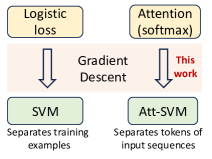
Figure 3: Implicit biases of the attention layer and logistic regression.

Unveiling the relationship between attention and linear SVMs. For linear classification, it is well-established that GD iterations on logistic loss and separable datasets converge towards the hard margin SVM solution, which effectively separates the two classes within the data [SHN⁺18, RZH03, ZY05]. The softmax nonlinearity employed by the attention layer exhibits an exponentially-tailed behavior similar to the logistic loss; thus, attention may also be biased towards margin-maximizing solutions. However, the attention layer operates on tokens within an input sequence, rather than performing classification directly. Therefore, its bias is towards an SVM, specifically (Att-SVM), which aims to separate the tokens of input sequences by selecting the relevant ones and suppressing the rest. Nonetheless, formalizing this intuition is considerably more challenging: The presence of the highly nonlinear and nonconvex softmax operation renders the analysis of standard GD algorithms intricate. Additionally, the 1-layer transformer in (2) does not inherently exhibit a singular bias towards a single (Att-SVM) problem, even when using a linear head $h$. Instead, it can result in multiple locally optimal directions induced by their associated SVMs. We emphasize that [TLZO23] is the first work to make this attention$\leftrightarrow$SVM connection. Here, we augment their framework to transformers by developing the first guarantees for self/cross-attention layer, nonlinear prediction heads, and global convergence.

Notation. For any integer $N\geq 1$, let $[N]:=\{1,\dots,N\}$. We use lowercase and uppercase bold letters (e.g., ${\bm{a}}$ and ${\bm{A}}$) to represent vectors and matrices, respectively. The entries of a vector ${\bm{a}}$ are denoted as ${\bm{a}}_{i}$. For a matrix ${\bm{A}}$, $\|{{\bm{A}}}\|$ denotes the spectral norm, i.e. maximum singular value, $\|{{\bm{A}}}\|_{\star}$ denotes the nuclear norm, i.e. summation of all singular values, and $\|{{\bm{A}}}\|_{F}:=\sqrt{{{\operatorname{trace}}}({\bm{A}}^{\top}{\bm{A}})}$ denotes the Frobenius norm. $\texttt{dist}\left(\cdot,\cdot\right)$ denotes the Euclidean distance between two sets. The minimum / maximum of two numbers $a$, $b$ is denoted as $a\wedge b$ / $a\vee b$. The big-O notation $\mathcal{O}(\cdot)$ hides the universal constants.

Optimization problem definition. We use a linear head $h(\bm{x})=\bm{v}^{\top}\bm{x}$ for most of our theoretical exposition. Given dataset $(Y_{i},{\bm{X}}_{i},{\bm{z}}_{i})_{i=1}^{n}$, we minimize the empirical risk of an 1-layer transformer using combined weights $\bm{W}\in\mathbb{R}^{d\times d}$ or individual weights ${\bm{K}},{\bm{Q}}\in\mathbb{R}^{d\times m}$ for a fixed head and decreasing loss function:

$${\cal{L}}(\bm{W}) =\frac{1}{n}\sum_{i=1}^{n}\ell\left(Y_{i}\cdot\bm{v}^{\top}{\bm{X}}_{i}^{\top}\mathbb{S}({\bm{X}}_{i}\bm{W}{\bm{z}}_{i})\right),$$ (W-ERM)

$${\cal{L}}({\bm{K}},{\bm{Q}}) =\frac{1}{n}\sum_{i=1}^{n}\ell\left(Y_{i}\cdot\bm{v}^{\top}{\bm{X}}_{i}^{\top}\mathbb{S}({\bm{X}}_{i}{\bm{K}}{\bm{Q}}^{\top}{\bm{z}}_{i})\right).$$ (KQ-ERM)

We can recover the self-attention model by setting ${\bm{z}}_{i}$ to be the first token of ${\bm{X}}_{i}$, i.e., ${\bm{z}}_{i}\leftarrow\bm{x}_{i1}$. While the above formulation regresses a single label $Y_{i}$ per $({\bm{X}}_{i},{\bm{z}}_{i})$, in Sections 6 and E, we show that our findings gracefully extend to the sequence-to-sequence classification setting where we output and classify $T$ tokens per inputs ${\bm{X}}_{i},\bm{Z}_{i}\in\mathbb{R}^{T\times d}$. See Sections 6 and E for results on nonlinear prediction heads.

Optimization algorithms. Given a parameter $R>0$, we consider an $\ell_{2}$-norm bound $R$, and define the regularized path solution associated with Objectives (W-ERM) and (KQ-ERM), respectively as (W-RP) and (KQ-RP). These update rules allow us to find the solution within a constrained region defined by the norm bound. The RP illustrates the evolution of ${\bm{\bar{W}}}_{R}$ as $R$ increases, capturing the essence of GD where the ridge constraint serves as an approximation for the number of iterations. Previous studies, including [RZH03, SPR18, JDST20, TLZO23], have examined the implicit bias of logistic regression and established a connection between the directional convergence of the RP (i.e., $\lim_{R\rightarrow\infty}{\bm{\bar{W}}}_{R}/R$) and GD. In [TLZO23], the concept of a local RP was also employed to investigate implicit bias along local directions. For GD, with appropriate initialization and step size $\eta>0$, we describe the optimization process associated with (W-ERM) and (KQ-ERM) as (W-GD) and (KQ-GD), respectively.

2.1 Optimal tokens and hard-margin SVM problem for cross attention

Given ${\bm{X}}_{i}\in\mathbb{R}^{T\times d},{\bm{z}}_{i}\in\mathbb{R}^{d}$, we present a convex hard-margin SVM problem, denoted as (Att-SVM), that aims to separate a specific token from the remaining tokens in the input sequence ${\bm{X}}_{i}$. This problem is jointly solved for all inputs, allowing us to examine the optimization properties of cross-attention. To delve deeper, we introduce the concept of optimal tokens, which are tokens that minimize the training objective under the decreasing loss function $\ell(\cdot)$ as shown in Lemma 2. This exploration will introduce the notions of token scores and optimality, providing insights into the underlying principles of self-attention mechanisms [TLZO23].

Definition 1 (Token Score and Optimality)

Given a prediction head $\bm{v}\in\mathbb{R}^{d}$, the score of a token $\bm{x}_{it}$ of input ${\bm{X}}_{i}$ is defined as $\bm{\gamma}_{it}=Y_{i}\cdot\bm{v}^{\top}\bm{x}_{it}$. The optimal token for each input ${\bm{X}}_{i}$ is given by the index $\texttt{opt}_{i}\in\arg\max_{t\in[T]}\bm{\gamma}_{it}$ for all $i\in[n]$.

By introducing token scores and identifying optimal tokens, we can better understand the importance of individual tokens and their impact on the overall objective. The token score quantifies the contribution of a token to the prediction or classification task, while the optimal token represents the token that exhibits the highest relevance within the corresponding input sequence.

$\bullet$ Hard-margin SVM for $\bm{W}$-parameterization. Equipped with the set of optimal indices $\texttt{opt}:=(\texttt{opt}_{i})_{i=1}^{n}$ as per Definition 1, we introduce the following SVM formulation associated to (W-ERM):

The existence of matrix $\bm{W}^{\textsl{mm}}$ implies the separability of tokens $(\texttt{opt}_{i})_{i=1}^{n}$ from the others. The terms $a_{{it}}:=\bm{x}_{it}^{\top}\bm{W}{\bm{z}}_{i}$ represent the dot product between the key-query features before applying the softmax nonlinearity. This dot product is a crucial characteristic of self-attention and we can express the SVM constraints in (Att-SVM) as $a_{i\texttt{opt}_{i}}\geq a_{it}+1$. Thus, (Att-SVM) finds the most efficient direction that ensures the optimal token $\bm{x}_{i\texttt{opt}_{i}}$ achieves the highest similarity with query ${\bm{z}}_{i}$ among all key embeddings. Our first result shows that (Att-SVM) is feasible under mild over-parameterization.

Theorem 1

Suppose $d\geq\max(T-1,n)$. Then, almost all datasets $(Y_{i},{\bm{X}}_{i},{\bm{z}}_{i})_{i=1}^{n}$ – including the self-attention setting with ${\bm{z}}_{i}\leftarrow\bm{x}_{i1}$ – obey the following: (Att-SVM) is feasible i.e., $\bm{W}^{\textsl{mm}}$ separates the desired tokens $\texttt{opt}=(\texttt{opt}_{i})_{i=1}^{n}$.

We note that the convex formulation (Att-SVM) does not fully capture the GD geometry on (W-ERM). In a more general sense, GD can provably converge to an SVM solution over locally-optimal tokens, as detailed in Section 5.1. For deeper insight into (Att-SVM), consider that the attention layer’s output is a convex mixture of input tokens. Thus, if minimizing the training loss involves choosing the optimal token $\bm{x}_{i\texttt{opt}_{i}}$, the softmax similarities should eventually converge to a one-hot vector, precisely including $\bm{x}_{i\texttt{opt}_{i}}$ (assigned 1), while ignoring all other tokens (assigned 0s). This convergence requires the attention weights $\bm{W}$ to diverge in norm to saturate the softmax probabilities. Due to the exponential-tailed nature of the softmax function, the weights converge directionally to the max-margin solution. This phenomenon resembles the implicit bias of logistic regression on separable data [SHN⁺18, JT18]. Lemma 2 formalizes this intuition and rigorously motivates optimal tokens.

$\bullet$ Non-convex SVM for $({\bm{K}},{\bm{Q}})$-parameterization. The objective function (KQ-ERM) has an extra layer of nonconvexity compared to (W-ERM) as $({\bm{K}},{\bm{Q}})$ corresponds to a matrix factorization of $\bm{W}$. To study this, we introduce the following nonconvex SVM problem over $({\bm{K}},{\bm{Q}})$ akin to (Att-SVM):

Even if the direction of GD is biased towards the SVM solution, it does not have to converge to the global minima of (KQ-SVM). Instead, it can converge towards a Karush–Kuhn–Tucker (KKT) point of the max-margin SVM. Such KKT convergence has been studied by [LL19, JT20] in the context of other nonconvex margin maximization problems. Fortunately, (KQ-ERM) may not be as daunting as it may initially seem: Our experiments in Figures 2 and 7 reveal that GD is indeed biased towards the global minima of (KQ-SVM). This global minima is achieved by setting $\bm{W}:={\bm{K}}{\bm{Q}}^{\top}$ and finding the factorization of $\bm{W}$ that minimizes the quadratic objective, yielding the following $\bm{W}$-parameterized SVM with nuclear norm objective:

Above, the nonconvex rank constraint arises from the fact that the rank of $\bm{W}={\bm{K}}{\bm{Q}}^{\top}$ is at most $m$. However, under the condition of the full parameterization where $m\geq d$, the rank constraint disappears, leading to a convex nuclear norm minimization problem. Besides, the nuclear norm objective inherently encourages a low-rank solution [RFP10, Faz02, SRJ04]. Lemma 1, presented below, demonstrates that this guarantee holds whenever $n\leq m$. This observation is further supported by our experiments (see Fig. 4). Thus, it offers a straightforward rationale for why setting $m<d$ is a reasonable practice, particularly in scenarios involving limited data.

Lemma 1

Any optimal solution of (Att-SVM) or (Att-SVM_⋆) is at most rank $n$. More precisely, the row space of $\bm{W}^{\textsl{mm}}$ or $\bm{W}^{\textsl{mm}}_{\star}$ lies within $\texttt{span}(\{{\bm{z}}_{i}\}_{i=1}^{n})$.

Figure 4 illustrates rank range of solutions for (Att-SVM) and (Att-SVM_⋆), denoted as $\bm{W}^{\textsl{mm}}$ and $\bm{W}^{\textsl{mm}}_{\star}$, solved using optimal tokens $(\texttt{opt}_{i})_{i=1}^{n}$ and setting $m=d$ (the rank constraint is eliminated). Each result is averaged over 100 trials, and for each trial, ${\bm{x}}_{it}$, ${{\bm{z}}}_{i}$, and linear head ${\bm{v}}$ are randomly sampled from the unit sphere. In Fig. 4(a), we fix $T=5$ and vary $n$ across $\{5,10,15\}$. Conversely, in Fig. 4(b), we keep $n=5$ constant and alter $T$ across $\{5,10,15\}$. Both figures confirm rank of $\bm{W}^{\textsl{mm}}$ and $\bm{W}^{\textsl{mm}}_{\star}$ are bounded by $\max(n,d)$, validating Lemma 1.

(a) Rank of attention SVM solutions with fixed $T=5$

(b) Rank of attention SVM solutions with fixed $n=5$

Figure 4: Rank range of solutions for (Att-SVM) and (Att-SVM_⋆), denoted as $\bm{W}^{\textsl{mm}}$ and $\bm{W}^{\textsl{mm}}_{\star}$, solved using optimal tokens $(\texttt{opt}_{i})_{i=1}^{n}$ and setting $m=d$ (the rank constraint is eliminated). Both figures confirm ranks of $\bm{W}^{\textsl{mm}}$ and $\bm{W}^{\textsl{mm}}_{\star}$ are bounded by $\max(n,d)$, validating Lemma 1.

3 Understanding the Implicit Bias of Self-Attention

We start by motivating the optimal token definition and establishing the global convergence of RPs which shed light on the implicit bias of attention parameterizations. Throughout, we maintain the following assumption regarding the loss function.

Assumption A

Over any bounded interval $[a,b]$: (i) $\ell:\mathbb{R}\rightarrow\mathbb{R}$ is strictly decreasing; (ii) The derivative $\ell^{\prime}$ is bounded as $|\ell^{\prime}(u)|\leq M_{1}$; (iii) $\ell^{\prime}$ is $M_{0}$-Lipschitz continuous.

Assumption A encompasses many common loss functions, e.g., logistic $\ell\left(u\right)=\log\left(1+e^{-u}\right)$, exponential $\ell\left(u\right)=e^{-u}$, and correlation $\ell(u)=-u$ losses.

Lemma 2 (Optimal Tokens Minimize Training Loss)

Suppose Assumption A (i)-(ii) hold, and not all tokens are optimal per Definition 1. Then, training risk obeys ${\cal{L}}(\bm{W})>{\cal{L}}_{\star}:=\frac{1}{n}\sum_{i=1}^{n}\ell(\bm{\gamma}_{i\texttt{opt}_{i}})$. Additionally, suppose there are optimal indices $(\texttt{opt}_{i})_{i=1}^{n}$ for which (Att-SVM) is feasible, i.e. there exists a $\bm{W}$ separating optimal tokens. This $\bm{W}$ choice obeys $\lim_{R\rightarrow\infty}{\cal{L}}(R\cdot\bm{W})={\cal{L}}_{\star}$.

The result presented in Lemma 2 originates from the observation that the output tokens of the attention layer constitute a convex combination of the input tokens. Consequently, when subjected to a strictly decreasing loss function, attention optimization inherently leans towards the selection of a singular token, specifically, the optimal token $(\texttt{opt}_{i})_{i=1}^{n}$. Our following theorem unveils the implicit bias ingrained within both attention parameterizations through RP analysis.

Theorem 2

Suppose Assumptions A holds, optimal indices $(\texttt{opt}_{i})_{i=1}^{n}$ are unique, and (Att-SVM) is feasible. Let $\bm{W}^{\textsl{mm}}$ be the unique solution of (Att-SVM), and let ${\cal{W}}^{\textsl{mm}}_{\star}$ be the solution set of (Att-SVM_⋆) with nuclear norm achieving objective $C_{\star}$. Then, Algorithms W-RP and KQ-RP, respectively, satisfy:

• $\bm{W}$-parameterization has Frobenius norm bias: $\underset{R\rightarrow\infty}{\lim}\frac{{\bm{\bar{W}}}_{R}}{R}=\frac{\bm{W}^{\textsl{mm}}}{\|{\bm{W}^{\textsl{mm}}}\|_{F}}$.

• $({\bm{K}},{\bm{Q}})$-parameterization has nuclear norm bias: $\underset{R\rightarrow\infty}{\lim}\texttt{dist}\left(\frac{{\bm{\bar{K}}}_{R}{\bm{\bar{Q}}}_{R}^{\top}}{R},\frac{{\cal{W}}^{\textsl{mm}}_{\star}}{C_{\star}}\right)=0$.

  • Setting $m=d$: (Att-SVM_⋆) is a convex problem without rank constraints.

Theorem 2 demonstrates that the RP of the $({\bm{K}},{\bm{Q}})$-parameterization converges to a max-margin solution of (Att-SVM_⋆) with nuclear norm objective on $\bm{W}={\bm{K}}{\bm{Q}}^{\top}$. When self-attention is directly parameterized by $\bm{W}$, the RP converges to the solution of (Att-SVM) with a Frobenius norm objective. This result is the first to distinguish the optimization dynamics of $\bm{W}$ and $({\bm{K}},{\bm{Q}})$ parameterizations, revealing the low-rank bias of the latter. These findings also provide a clear characterization of token optimality (Definition 1) and extend naturally to the setting with multiple optimal tokens per sequence (Theorem 9 in appendix). By definition, the RP captures the global geometry and cannot be used for the implicit bias of GD towards locally-optimal directions. Sections 4 and 5 accomplish this goal through gradient-descent and localized RP analysis to obtain locally-applicable SVM equivalences. Note that, this theorem requires each input sequence has a unique optimal token per Definition 1. Fortunately, this is a very mild condition as it holds for almost all datasets, namely, as soon as input features are slightly perturbed.

Theorem 2 establishes the implicit bias of attention from the perspective of RP analysis. This leads to the question: To what extent is this RP theory predictive of the implicit bias exhibited by GD? To delve into this, we examine the gradient paths of $\bm{W}(k)$ or $({\bm{K}}(k),{\bm{Q}}(k))$ and present the findings in Figure 2. We consider a scenario where $n=d=m=2$ and $T=5$, and employ cross-attention, where tokens $({\bm{z}}_{1},{\bm{z}}_{2})$ are generated independently of the inputs $({\bm{X}}_{1},{\bm{X}}_{2})$. The teal and yellow markers correspond to tokens from ${\bm{X}}_{1}$ and ${\bm{X}}_{2}$, respectively. The stars indicate the optimal token for each input. To provide a clearer view of the gradient convergence path, we illustrate the outcomes of training the attention weight $\bm{W}$ or $({\bm{K}},{\bm{Q}})$ in the form of $\bm{W}{\bm{z}}_{i}$ or ${\bm{K}}{\bm{Q}}^{\top}{\bm{z}}_{i}$, where $i={1,2}$. With reference to Equations (Att-SVM) and (Att-SVM_⋆), the red and blue solid lines in Fig. 1(a) delineate the directions of $\bm{W}^{\textsl{mm}}{\bm{z}}_{1}$ and $\bm{W}^{\textsl{mm}}{\bm{z}}_{2}$, correspondingly. Conversely, the red and blue solid lines in Fig. 1(b) show the directions of $\bm{W}^{\textsl{mm}}_{\star}{\bm{z}}_{1}$ and $\bm{W}^{\textsl{mm}}_{\star}{\bm{z}}_{2}$. The red/blue arrows denote the corresponding directions of gradient evolution with the dotted lines representing the corresponding separating hyperplanes. Figure 2 provides a clear depiction of the incremental alignment of $\bm{W}(k)$ and ${\bm{K}}(k){\bm{Q}}(k)^{\top}$ with their respective attention SVM solutions as $k$ increases. This strongly supports the assertions of Theorem 2.

It is worth noting that (Att-SVM_⋆) imposes a nonconvex rank constraint, i.e., $\texttt{rank}(\bm{W})\leq m$. Nevertheless, this constraint becomes inconsequential if the unconstrained problem, with $m$ set to be greater than or equal to $d$, admits a low-rank solution, as demonstrated in Lemma 1. Consequently, in our experimental endeavors, we have the flexibility to employ the unconstrained attention SVM for predicting the implicit bias. This concept is succinctly summarized by the following lemma.

Lemma 3

Let ${\cal{W}}^{\textsl{mm}}_{\star}$ be the solution set of (Att-SVM_⋆) with nuclear norm achieving objective $C_{\star}$. Further let ${\cal{W}}^{\textsl{mm}}_{\texttt{cvx}}$ be the solution set of (Att-SVM_⋆) with $m=d$ achieving objective $C_{\texttt{cvx}}$. If ${\cal{W}}^{\textsl{mm}}_{\star}\cap{\cal{W}}^{\textsl{mm}}_{\texttt{cvx}}\neq\emptyset$, then $C_{\star}=C_{\texttt{cvx}}$ and ${\cal{W}}^{\textsl{mm}}_{\star}\subseteq{\cal{W}}^{\textsl{mm}}_{\texttt{cvx}}$. Also, if the elements of ${\cal{W}}^{\textsl{mm}}_{\texttt{cvx}}$ have rank at most $m$, then, ${\cal{W}}^{\textsl{mm}}_{\star}={\cal{W}}^{\textsl{mm}}_{\texttt{cvx}}$.

4 Global Convergence of Gradient Descent

In this section, we will establish conditions that guarantee the global convergence of GD. Concretely, we will investigate when GD solution selects the optimal token within each input sequence through the softmax nonlinearity and coincides with the solution of the RP. Section 5 will complement this with showing that self-attention can more generally converge to locally-optimal max-margin directions. We identify the following conditions as provable catalysts for global convergence: (i) Optimal tokens have relatively large scores; (ii) Initial gradient direction is favorable; (iii) Overparameterization, i.e. $d$ is appropriately large.

4.1 Properties of optimization landscape

We start by establishing some fundamental properties of Objectives (W-ERM) and (KQ-ERM).

Lemma 4

Under Assumption A, $\nabla{\cal{L}}(\bm{W})$, $\nabla_{{\bm{K}}}{\cal{L}}({\bm{K}},{\bm{Q}})$, and $\nabla_{{\bm{Q}}}{\cal{L}}({\bm{K}},{\bm{Q}})$ are $L_{\bm{W}}$, $L_{{\bm{K}}}$, $L_{{\bm{Q}}}$–Lipschitz continuous, respectively, where $a_{i}=\|\bm{v}\|~{}\|{\bm{z}}_{i}\|^{2}\|{\bm{X}}_{i}\|^{3}$, $b_{i}=M_{0}\|\bm{v}\|~{}\|{\bm{X}}_{i}\|+3M_{1}$ for all $i\in[n]$,

$$L_{\bm{W}}:=\frac{1}{n}\sum_{i=1}^{n}a_{i}b_{i},\quad L_{{\bm{K}}}:=\|{\bm{Q}}\|L_{\bm{W}},\quad\textnormal{and}\quad L_{{\bm{Q}}}:=\|{\bm{K}}\|L_{\bm{W}}.$$ (3)

The next assumption will play an important role ensuring the attention layer has a benign optimization landscape.

Assumption B

Optimal tokens’ indices $(\texttt{opt}_{i})_{i=1}^{n}$ are unique and one of the following conditions on the tokens holds:

1. All tokens are support vectors, i.e., $(\bm{x}_{i\texttt{opt}_{i}}-\bm{x}_{it})^{\top}\bm{W}^{\textsl{mm}}{\bm{z}}_{i}=1$ for all $t\neq\texttt{opt}_{i}$ and $i\in[n]$.

2. The tokens’ scores, as defined in Definition 1, satisfy $\bm{\gamma}_{it}=\bm{\gamma}_{i\tau}<\bm{\gamma}_{i\texttt{opt}_{i}}$, for all $t,\tau\neq\texttt{opt}_{i}$ and $i\in[n]$.

Assumption B.1 is directly linked to overparameterization and holds practical significance. In scenarios such as classical SVM classification, where the goal is to separate labels, overparameterization leads to the situation where all training points become support vectors. Consequently, the SVM solution aligns with the least-squares minimum-norm interpolation, a concept established in [MNS⁺21, HMX21] under broad statistical contexts. Assumption B.1 represents an analogous manifestation of this condition. Therefore, in cases involving realistic data distributions with sufficiently large $d$, we expect the same phenomena to persist, causing the SVM solution $\bm{W}^{\textsl{mm}}$ to coincide with (Att-SVM).

Drawing on insights from [HMX21, Theorem 1] and our Theorem 1, we expect that the necessary degree of overparameterization remains moderate. Specifically, in instances where input sequences follow an independent and identically distributed (IID) pattern and tokens exhibit IID isotropic distributions, we posit that $d\gtrsim(T+n)\log(T+n)$ will suffice. More generally, the extent of required overparameterization will be contingent on the covariance of tokens [BLLT20, MNS⁺21] and the distribution characteristics of input sequences [WT22].

Assumption B.2 stipulates that non-optimal tokens possess identical scores which constitutes a relatively stringent assumption that we will subsequently relax. Under Assumption B, we establish that when optimization problem (W-ERM) is trained using GD, the norm of parameters will diverge.

Theorem 3

Suppose Assumption A on the loss function $\ell$ and Assumption B on the tokens hold.

• There is no $\bm{W}\in\mathbb{R}^{d\times d}$ satisfying $\nabla{\cal{L}}(\bm{W})=0$.

• Algorithm W-GD with the step size $\eta\leq 1/L_{\bm{W}}$ and any starting point $\bm{W}(0)$ satisfies $\lim_{k\rightarrow\infty}\|{\bm{W}(k)}\|_{F}=\infty$.

The feasibility of SVM (per Theorem 1) is a necessary condition for the convergence of GD to the $\bm{W}^{\textsl{mm}}$ direction. However, it does not inform us about the optimization landscape. Two additional criteria are essential for convergence: the absence of stationary points $\nabla{\cal{L}}(\bm{W})=0$ and divergence of parameter norm to infinity. Theorem 3 above precisely guarantees both of these criteria under Assumption B.

(a) Convergence behaviour of GD for $\bm{W}$-parameterization

(b) Convergence behaviour of GD for $({\bm{K}},{\bm{Q}})$-parameterization

Figure 5: Percentage of different convergence types of GD when training cross-attention weights (a): $\bm{W}$ or (b): $({\bm{K}},{\bm{Q}})$ with varying $d$. In both figures, red, blue, and teal bars represent the percentages of Global, Local (including Global), and Not Local convergence, respectively. The green bar corresponds to Assumption B.1 where all tokens act as support vectors. Larger overparameterization ($d$) relates to a higher percentage of globally-optimal SVM convergence.

4.2 Provable global convergence of 1-layer transformer

In the quest for understanding the global convergence of a 1-layer transformer, [TLZO23, Theorem 2] provided the first global convergence analysis of the attention in a restrictive scenario where $n=1$ and under the assumption B.2. Here, we present two new conditions for achieving global convergence towards the max-margin direction $\bm{W}^{\textsl{mm}}$ based on: (I) the initial gradient direction, and (II) over-parameterization. For the first case, we provide precise theoretical guarantees. For the second, we offer strong empirical evidence, supported by Theorem 3, and a formal conjecture described in Section 5.2. We remind the reader that we optimize the attention weights $\bm{W}$ while fixing the linear prediction head $h(\bm{x})=\bm{v}^{\top}\bm{x}$. This approach avoids trivial convergence guarantees where an over-parameterized $h(\cdot)$—whether it is a linear model or an MLP—can be used to achieve zero training loss without providing any meaningful insights into the functionality of the attention mechanism.

(I) Global convergence under good initial gradient.

To ensure global convergence, we identify an assumption that prevents GD from getting trapped at suboptimal tokens that offer no scoring advantage compared to other choices. To establish a foundation for providing the convergence of GD to the globally optimal solution $\bm{W}^{\textsl{mm}}$, we need the following definitions. For parameters $\mu>0$ and $R>0$, define

$$\bar{\mathcal{C}}_{\mu,R}:=\Bigg{\{}\|{\bm{W}}\|_{F}\geq R~{}\Big{|}~{}\left<(\bm{x}_{i\texttt{opt}_{i}}-\bm{x}_{it}){\bm{z}}_{i}^{\top},\frac{\bm{W}}{\|{\bm{W}}\|_{F}}\right>\geq\mu\quad\textnormal{for all}\quad t\neq\texttt{opt}_{i},~{}i\in[n]\Bigg{\}}.$$ (4)

This is the set of all $\bm{W}$s that separate the optimal tokens from the rest with margin $\mu$. We will show that, for any $\mu>0$, the optimization landscape of this set is favorable and, if the updates remain in the set, the gradient descent will maximize the margin and find $\bm{W}^{\textsl{mm}}$.

Assumption C (First GD Step is Separating)

For some $\iota>0$ and all $t\neq\texttt{opt}_{i},~{}i\in[n]$: $(\bm{x}_{it}-\bm{x}_{i\texttt{opt}_{i}})^{\top}\nabla{\cal{L}}(0){\bm{z}}_{i}\geq\iota$.

Theorem 4

Suppose Assumption A on the loss function $\ell$ and Assumption C on the initial gradient hold.

• For any $\mu>0$, there exists $R>0$ such that $\bar{\mathcal{C}}_{\mu,R}$ does not contain any stationary points.

• Fix any $\mu\in(0,\iota/\|{\nabla{\cal{L}}(0)}\|_{F})$. Consider GD iterations with $\bm{W}(0)=0$, $\bm{W}(1)=-R\nabla\,{\cal{L}}(0)/\|{\nabla{\cal{L}}(0)}\|_{F}$, and $\bm{W}(k+1)=\bm{W}(k)-\eta\nabla{\cal{L}}(\bm{W}(k))$ for $k\geq 1$, where $\eta\leq 1/L_{\bm{W}}$ and $R$ sufficiently large. If all iterates remain within $\bar{\mathcal{C}}_{\mu,R}$, then $\lim_{k\rightarrow\infty}\|{\bm{W}(k)}\|_{F}=\infty$ and $\lim_{k\rightarrow\infty}\frac{\bm{W}(k)}{\|{\bm{W}(k)}\|_{F}}=\frac{\bm{W}^{\textsl{mm}}}{\|{\bm{W}^{\textsl{mm}}}\|_{F}}$.

Note that the second result of Theorem 4, i.e., the divergence of parameter norm to infinity and directional convergence requires that all GD iterations remain within $\bar{\mathcal{C}}_{\mu,R}$ defined in (4). In Appendix C.2, we show that if for all $\bm{W}\in\bar{\mathcal{C}}_{\mu,R}(\bm{W}^{\textsl{mm}})$, $\min_{i\in[n]}\left<(\bm{x}_{i\texttt{opt}_{i}}-\bm{x}_{it}){\bm{z}}_{i}^{\top},\bm{W}-\eta\nabla{\cal{L}}(\bm{W})\right>-\min_{i\in[n]}\left<(\bm{x}_{i\texttt{opt}_{i}}-\bm{x}_{it}){\bm{z}}_{i}^{\top},\bm{W}\right>$ is lower bounded by $(2\eta\mu/\|{\bm{W}^{\textsl{mm}}}\|_{F})\left\langle-\nabla\mathcal{L}(\bm{W}),\bm{W}^{\textsl{mm}}\right\rangle$, then all GD iterations $\bm{W}(k)$ remain within $\bar{\mathcal{C}}_{\mu,R}$. While this condition may appear complicated, it is essentially a tight requirement for updates to remain within $\bar{\mathcal{C}}_{\mu,R}$. Finally, it is worth mentioning that, if a stronger correlation condition between initial gradient $\nabla{\cal{L}}(0)$ and $\bm{W}^{\textsl{mm}}$ holds, one can also prove that updates remain within a tighter cone around $\bm{W}^{\textsl{mm}}$ through ideas developed in Theorem 5 by landing $\bm{W}(1)$ around $\bm{W}^{\textsl{mm}}$ direction. However, we opt to state here the result for the milder condition $\bar{\mathcal{C}}_{\mu,R}$.

(a) Global convergence for varying $n,d$

(b) Global convergence for varying $T,d$

Figure 6: Global convergence behavior of GD when training cross-attention weights $\bm{W}$ (solid) or $({\bm{K}},{\bm{Q}})$ (dashed) with random data. The blue, green, and red curves represent the probabilities of global convergence for (a): fixing $T=5$ and varying $n\in\{5,10,20\}$ and (b): fixing $n=5$ and varying $T\in\{5,10,20\}$. Results demonstrate that for both attention models, as $d$ increases (due to over-parameterization), attention weights tend to select optimal tokens $(\texttt{opt}_{i})_{i=1}^{n}$.

(II) Global convergence via overparameterization.

In the context of standard neural networks, overparameterization has been recognized as a pivotal factor for the global convergence of GD [DZPS18, AZLS19, LL18, OS19]. However, conventional approaches like the neural tangent kernel [JGH18] do not seamlessly apply to our scenario, given our assumption on fixed $h$ and the avoidance of achieving zero loss by trivially fitting $h$. Furthermore, even when we train $h$ to achieve zero loss, it doesn’t provide substantial insights into the implicit bias of the attention weights $\bm{W}$. Conversely, Theorem 3 illustrates the benefits of over-parameterization in terms of convergence. Considering that Assumption B.1 is anticipated to hold as the dimension $d$ increases, the norm of the GD solution is bound to diverge to infinity. This satisfies a prerequisite for converging towards the globally-optimal SVM direction $\bm{W}^{\textsl{mm}}$.

The trend depicted in Figure 5, where the percentage of global convergence (red bars) approaches $100\%$ and Assumption B.1 holds with higher probability (green bars) as $d$ grows, reinforces this insight. Specifically, Fig. 5(a) is similar to Figure 2 but with additional green bars representing the percentage of the scenarios where almost all tokens act as support vectors (Assumption B.1), and Fig. 5(b) displays the same evaluation over $({\bm{K}},{\bm{Q}})$-parameterization setting. In both experiments, and for each chosen $d$ value, a total of $500$ random instances are conducted under the conditions of $n=T=5$. The outcomes are reported in terms of the percentages of Not Local, Local, and Global convergence, represented by the teal, blue, and red bars, respectively. We validate Assumption B.1 as follows: Given a problem instance, we compute the average margin over all non-optimal tokens of all inputs and declare that problem satisfies Assumption B.1, if the average margin is below 1.1 (where 1 is the minimum).

Furthermore, the observations in Figure 6 regarding the percentages of achieving global convergence reaching 100 with larger $d$ reaffirm that overparameterization leads the attention weights to converge directionally towards the optimal max-margin direction outlined by (Att-SVM) and (Att-SVM_⋆).

In the upcoming section, we will introduce locally-optimal directions, to which GD can be proven to converge when appropriately initialized. We will then establish a condition that ensures the globally-optimal direction is the sole viable locally-optimal direction. This culmination will result in a formal conjecture detailed in Section 5.2.

5 Understanding Local Convergence of 1-Layer Transformer

So far, we have primarily focused on the convergence to the global direction dictated by (Att-SVM). In this section, we investigate and establish the local directional convergence of GD as well as RP.

(a) Evolution of softmax probabilities

(b) Corr. coeff. of GD and $\bm{W}^{\textsl{mm}}_{\bm{\alpha}}$

(c) Corr. coeff. of GD and $\bm{W}^{\textsl{mm}}_{\star,{\bm{\alpha}}}$

Figure 7: Local convergence behaviour of GD when training cross-attention weights $\bm{W}$ (blue) or $({\bm{K}},{\bm{Q}})$ (red) with random data: (a) displays the largest entry of the softmax outputs averaged over the dataset; (b&c) display the Pearson correlation coefficients of GD trajectories and the SVM solutions (b) with the Frobenius norm objective $\bm{W}^{\textsl{mm}}_{\bm{\alpha}}$ (solution of (Att-SVM)) and (c) with the nuclear norm objective $\bm{W}^{\textsl{mm}}_{\star,{\bm{\alpha}}}$ (solution of (Att-SVM_⋆)). These demonstrate the Frobenius norm bias of $\bm{W}(k)$ and the nuclear norm bias of ${\bm{K}}(k){\bm{Q}}(k)^{\top}$.

5.1 Local convergence of gradient descent

To proceed, we introduce locally-optimal directions by adapting Definition 2 of [TLZO23].

Definition 2 (Support Indices and Locally-Optimal Direction)

Fix token indices ${\bm{\alpha}}=(\alpha_{i})_{i=1}^{n}$. Solve (Att-SVM) with $(\texttt{opt}_{i})_{i=1}^{n}$ replaced with $\bm{\alpha}=(\alpha_{i})_{i=1}^{n}$ to obtain $\bm{W}^{\textsl{mm}}_{\bm{\alpha}}$. Consider the set $\mathcal{T}_{i}\subset[T]$ such that $(\bm{x}_{i\alpha_{i}}-\bm{x}_{it})^{\top}\bm{W}^{\textsl{mm}}_{\bm{\alpha}}{\bm{z}}_{i}=1$ for all $t\in\mathcal{T}_{i}$. We refer to $(\mathcal{T}_{i})_{i=1}^{n}$ as the support indices of ${\bm{\alpha}}$. Additionally, if for all $i\in[n]$ and $t\in\mathcal{T}_{i}$ scores per Definition 1 obey $\bm{\gamma}_{i\alpha_{i}}>\bm{\gamma}_{it}$, indices ${\bm{\alpha}}=(\alpha_{i})_{i=1}^{n}$ are called locally-optimal and $\bm{W}^{\textsl{mm}}_{\bm{\alpha}}$ is called a locally-optimal direction.

In words, the concept of local optimality requires that the selected tokens denoted as ${\bm{\alpha}}$ should have scores that are higher than the scores of their neighboring tokens referred to as support indices. It is important to observe that the tokens defined as $\texttt{opt}=(\texttt{opt}_{i})_{i=1}^{n}$, which we term as the optimal tokens, inherently satisfy the condition of local optimality. Moving forward, we will provide Theorem 5 which establishes that when the process of GD is initiated along a direction that is locally optimal, it gradually converges in that particular direction, eventually aligning itself with $\bm{W}^{\textsl{mm}}_{\bm{\alpha}}$. This theorem immediately underscores the fact that if there exists a direction of local optimality (apart from the globally optimal direction $\bm{W}^{\textsl{mm}}$), then when GD commences from any arbitrary starting point, it does not achieve global convergence towards $\bm{W}^{\textsl{mm}}$.

To provide a basis for discussing local convergence of GD, we establish a cone centered around $\bm{W}^{\textsl{mm}}_{\bm{\alpha}}$ using the following construction. For parameters $\mu\in(0,1)$ and $R>0$, we define $\mathcal{C}_{\mu,R}(\bm{W}^{\textsl{mm}}_{\bm{\alpha}})$ as the set of matrices $\bm{W}\in\mathbb{R}^{d\times d}$ such that $\|{\bm{W}}\|_{F}\geq R$ and the correlation coefficient between $\bm{W}$ and $\bm{W}^{\textsl{mm}}_{\bm{\alpha}}$ is at least $1-\mu$:

$$\mathcal{C}_{\mu,R}({\bm{W}^{\textsl{mm}}_{\bm{\alpha}}})=\left\{\|{\bm{W}}\|_{F}\geq R~{}\Big{|}~{}\left\langle\frac{\bm{W}}{\|{\bm{W}}\|_{F}},\frac{\bm{W}^{\textsl{mm}}_{\bm{\alpha}}}{\|{{\bm{W}^{\textsl{mm}}_{\bm{\alpha}}}}\|_{F}}\right\rangle\geq 1-\mu\right\}.$$ (5)

Theorem 5

Suppose Assumption A on the loss $\ell$ holds, and let ${\bm{\alpha}}=(\alpha_{i})_{i=1}^{n}$ be locally optimal tokens according to Definition 2. Let $\bm{W}^{\textsl{mm}}_{\bm{\alpha}}$ denote the SVM solution obtained via (Att-SVM) by replacing $(\texttt{opt}_{i})_{i=1}^{n}$ with $\bm{\alpha}=(\alpha_{i})_{i=1}^{n}$.

• There exist parameters $\mu=\mu({\bm{\alpha}})\in(0,1)$ and $R>0$ such that $\mathcal{C}_{\mu,R}(\bm{W}^{\textsl{mm}}_{\bm{\alpha}})$ does not contain any stationary points.

• Algorithm W-GD with $\eta\leq 1/L_{\bm{W}}$ and any $\bm{W}(0)\in\mathcal{C}_{\mu,R}(\bm{W}^{\textsl{mm}}_{\bm{\alpha}})$ satisfies $\lim_{k\rightarrow\infty}\|{\bm{W}(k)}\|_{F}=\infty$ and $\lim_{k\rightarrow\infty}\frac{\bm{W}(k)}{\|{\bm{W}(k)}\|_{F}}=\frac{\bm{W}^{\textsl{mm}}_{\bm{\alpha}}}{\|{\bm{W}^{\textsl{mm}}_{\bm{\alpha}}}\|_{F}}$.

This theorem establishes the existence of positive parameters $\mu=\mu({\bm{\alpha}})>0$ and $R>0$ such that there are no stationary points within $\mathcal{C}_{\mu,R}(\bm{W}^{\textsl{mm}}_{\bm{\alpha}})$. Furthermore, if GD is initiated within $\mathcal{C}_{\mu,R}(\bm{W}^{\textsl{mm}}_{\bm{\alpha}})$, it will converge in the direction of $\bm{W}^{\textsl{mm}}_{\bm{\alpha}}/\|{\bm{W}^{\textsl{mm}}_{\bm{\alpha}}}\|_{F}$. It is worth mentioning that stronger Theorem 3 (e.g. global absence of stationary points) is applicable whenever all tokens are support i.e. $\bar{\mathcal{T}}_{i}=\emptyset$ for all $i\in[n]$.

In Figure 7, we consider setting where $n=6$, $T=8$, and $d=10$. The displayed results are averaged from $100$ random trials. We train cross-attention models with $\bm{x}_{it},{\bm{z}}_{i},\bm{v}\in\mathbb{R}^{d}$ randomly sampled from unit sphere, and apply the normalized GD approach with fixed step size $\eta=0.1$. In Figure 7(a) we calculate the softmax probability via $\frac{1}{n}\sum_{i=1}^{n}\max_{t\in[T]}\mathbb{S}({\bm{X}}_{i}\tilde{\bm{W}}(k){\bm{z}}_{i})_{t}$ for either $\tilde{\bm{W}}=\bm{W}$ or ${\bm{K}}{\bm{Q}}^{\top}$ at each iteration. Both scenarios result in probability $1$, which indicates that attention weights succeed in selecting one token per input. Then following Definition 2 let ${\bm{\alpha}}=(\alpha_{i})_{i=1}^{n}$ be the token indices selected by GD and denote $\bm{W}^{\textsl{mm}}_{\star,{\bm{\alpha}}}$ as the corresponding SVM solution of (Att-SVM_⋆). Define the correlation coefficient of two matrices as $\texttt{corr\_coef}(\bm{W}_{1},\bm{W}_{2}):=\left<\bm{W}_{1},\bm{W}_{2}\right>/\|\bm{W}_{1}\|_{F}\|\bm{W}_{2}\|_{F}$. Figures 7(b) and 7(c) illustrate the correlation coefficients of attention weights ($\bm{W}(k)$ and ${\bm{K}}(k){\bm{Q}}(k)^{\top}$) with respect to $\bm{W}^{\textsl{mm}}_{\bm{\alpha}}$ and $\bm{W}^{\textsl{mm}}_{\star,{\bm{\alpha}}}$. The results demonstrate that $\bm{W}$ (${\bm{K}}{\bm{Q}}^{\top}$) ultimately reaches a $1$ correlation with $\bm{W}^{\textsl{mm}}_{\bm{\alpha}}$ ($\bm{W}^{\textsl{mm}}_{\star,{\bm{\alpha}}}$), which suggests that $\bm{W}$ (${\bm{K}}{\bm{Q}}^{\top}$) converges in the direction of $\bm{W}^{\textsl{mm}}_{\bm{\alpha}}$ ($\bm{W}^{\textsl{mm}}_{\star,{\bm{\alpha}}}$). This further validates Theorem 5.

5.2 Overparameterization conjecture: When local-optimal directions disappear

In Section 4 we demonstrated that larger $d$ serves as a catalyst for global convergence to select the optimal indices $\texttt{opt}=(\texttt{opt}_{i})_{i=1}^{n}$. However, Section 5.1 shows that the convergence can be towards locally-optimal directions rather than global ones. How do we reconcile these? Under what precise conditions, can we expect global convergence?

The aim of this section is gathering these intuitions and stating a concrete conjecture on the global convergence of the attention layer under geometric assumptions related to overparameterization. To recap, Theorem 1 characterizes when (Att-SVM) is feasible and Theorem 3 characterizes when the parameter norm provably diverges to infinity, i.e. whenever all tokens are support vectors of (Att-SVM) (Assumption B.1 holds). On the other hand, this is not sufficient for global convergence, as GD can converge in direction to locally-optimal directions per Section 5.1. Thus, to guarantee global convergence, we need to ensure that globally-optimal direction is the only viable one. Our next assumption is a fully-geometric condition that precisely accomplishes this.

Assumption D (There is always an optimal support index)

For any choice of ${\bm{\alpha}}=(\alpha_{i})_{i=1}^{n}$ with ${\bm{\alpha}}\neq\texttt{opt}$ when solving (Att-SVM) with $\texttt{opt}\leftarrow{\bm{\alpha}}$, there exists $i\in[n]$ such that $\alpha_{i}\neq\texttt{opt}_{i}$ and $\texttt{opt}_{i}\in\mathcal{T}_{i}$.

This guarantees that no ${\bm{\alpha}}\neq\texttt{opt}$ can be locally-optimal because it has a support index with higher score at the input $i$ with $\alpha_{i}\neq\texttt{opt}_{i}$. Thus, this ensures that global direction $\bm{W}^{\textsl{mm}}$ is the unique locally-optimal direction obeying Def. 2. Finally, note that local-optimality in Def. 2 is one-sided: GD can provably converge to locally-optimal directions, while we do not provably exclude the existence of other directions. Yet, Theorem 4 of [TLZO23] shows that local RPs (see Section 5.4 for details) can only converge to locally-optimal directions for almost all datasets. This and Figure 5 provide strong evidence that Def. 2 captures all possible convergence directions of GD, and as a consequence, that Assumption D guarantees that $\bm{W}^{\textsl{mm}}$ is the only viable direction to converge.

➡ Integrating the results and global convergence conjecture. Combining Assumptions B.1 and D, we have concluded that gradient norm diverges and $\bm{W}^{\textsl{mm}}$ is the only viable direction to converge. Thus, we conclude this section with the following conjecture: Suppose $\texttt{opt}=(\texttt{opt}_{i})_{i=1}^{n}$ are the unique optimal indices with strictly highest score per sequence and Assumptions B.1 and D hold. Then, for almost all datasets (e.g. add small IID gaussian noise to input features), GD with a proper constant learning rate converges to $\bm{W}^{\textsl{mm}}$ of (Att-SVM) in direction.

To gain some intuition, consider Figure 5: Here, red bars denote the frequency of global convergence whereas green bars denote the frequency of Assumption B.1 holding over random problem instances. In short, this suggests that Assumption B.1 occurs less frequently than global convergence, which is consistent with our conjecture. On the other hand, verifying Assumption D is more challenging due to its combinatorial nature. A stronger condition that implies Assumption D is when all optimal indices $(\texttt{opt}_{i})_{i=1}^{n}$ are support vectors of the SVM. That is, either $\texttt{opt}_{i}=\alpha_{i}$ or $\texttt{opt}_{i}\in\mathcal{T}_{i}$, $\forall~{}i\in[n]$. When the data follows a statistical model, this stronger condition could be verified through probabilistic tools building on our earlier “all training points are support vectors” discussion [MNS⁺21]. More generally, we believe a thorough statistical investigation of (Att-SVM) is a promising direction for future work.

Figure 8: Performance of GD convergence and corresponding SVM margin. Upper: The SVM margins correspond to globally-optimal (red) and locally-optimal (blue) token indices, denoted as $1/\|{\bm{W}^{\textsl{mm}}}\|_{F}$ and $1/\|{\bm{W}^{\textsl{mm}}_{\bm{\alpha}}}\|_{F}$, respectively. Lower: Percentages of global convergence (when ${\bm{\alpha}}=\texttt{opt}$, red) and local convergence (when ${\bm{\alpha}}\neq\texttt{opt}$, blue).

5.3 Investigation on SVM objectives and GD convergence

Until now, we have discussed the global and local convergence performances of gradient descent (GD). Theorem 5 suggests that, without specific restrictions on tokens, when training with GD, the attention weight $\bm{W}$ converges towards $\bm{W}^{\textsl{mm}}_{\bm{\alpha}}$. Here, the selected token indices ${\bm{\alpha}}=(\alpha_{i})_{i=1}^{n}$ may not necessarily be identical to $\texttt{opt}=(\texttt{opt}_{i})_{i=1}^{n}$. Experiments presented in Figures 2, 5, and 6 also support this observation. In this section, we focus on scenarios where ${\bm{\alpha}}\neq\texttt{opt}$ (e.g., when $\bm{W}^{\textsl{mm}}$ is not feasible) and investigate the question: Towards which local direction is GD most likely to converge?

To this goal, in Figure 8, we consider SVM margin, which is defined by $1/\|{\bm{W}^{\textsl{mm}}_{\bm{\alpha}}}\|_{F}$, and investigate its connection to the convergence performance of GD. On the left, we set $T=d=5$ and vary $n$ among $1,5,10,15$; on the right, we fix $T=n=5$ and change $d$ to $2,5,10,15$. All tokens are randomly generated from the unit sphere. The SVM margins corresponding to the selected tokens ${\bm{\alpha}}$ are depicted as blue curves in the upper subfigures, while the SVM margins corresponding to the globally–optimal token indices (${\bm{\alpha}}=\texttt{opt}$) are shown as red curves. The red and blue bars in the lower subfigures represent the percentages of global and local convergence, respectively. Combining all these findings empirically demonstrates that when the global SVM objective yields a solution with a small margin (i.e., $1/\|{\bm{W}^{\textsl{mm}}}\|_{F}$ is small, and 0 when global SVM is not feasible), GD tends to converge towards a local direction with a comparatively larger margin.

5.4 Guarantees on local regularization path

In this section, we provide a localized regularization path analysis for general objective functions. As we shall see, this will also allow us to predict the local solutions of gradient descent described in Section 5.1. Let ${\diamond}$ denote a general norm objective. Given indices ${\bm{\alpha}}=(\alpha_{i})_{i=1}^{n}$, consider the formulation

$$\bm{W}^{\textsl{mm}}_{{\diamond},\alpha}=\underset{\texttt{rank}(W)\leq m}{\arg\min}\|\bm{W}\|_{\diamond}\quad\text{subj. to}\quad(\bm{x}_{i\alpha_{i}}-\bm{x}_{it})^{\top}\bm{W}{\bm{z}}_{i}\geq 1\quad\text{for all}\quad t\neq\alpha_{i},\quad i\in[n]. {\diamond}$$ (-SVM)

In this section, since ${\diamond}$ is clear from the context, we will use the shorthand $\bm{W}^{\textsl{mm}}_{\alpha}:=\bm{W}^{\textsl{mm}}_{{\diamond},\alpha}$ and denote the optimal solution set of (${\diamond}$-SVM) as ${\cal{W}}^{\textsl{mm}}:={\cal{W}}^{\textsl{mm}}_{{\diamond},\alpha}$. It is important to note that if the ${\diamond}$-norm is not strongly convex, ${\cal{W}}^{\textsl{mm}}$ may not be a singleton. Additionally, when $m=d$, the rank constraint becomes vacuous, and the problem becomes convex. The following result is a slight generalization of Theorem 1 and demonstrates that choosing a large $d$ ensures the feasibility of (${\diamond}$-SVM) uniformly over all choices of ${\bm{\alpha}}$. The proof is similar to that of Theorem 1, as provided in Appendix A.

Theorem 6

Suppose $d\geq\max(T-1,n)$ and $m=d$. Then, almost all datasets $(Y_{i},{\bm{X}}_{i},{\bm{z}}_{i})_{i=1}^{n}$ – including the self-attention setting with ${\bm{z}}_{i}\leftarrow\bm{x}_{i1}$ – obey the following: For any choice of indices ${\bm{\alpha}}=(\alpha_{i})_{i=1}^{n}\subset[T]$, (${\diamond}$-SVM) is feasible, i.e. the attention layer can separate and select indices ${\bm{\alpha}}$.

To proceed, we define the local regularization path, which is obtained by solving the ${\diamond}$-norm-constrained problem over a ${\bm{\alpha}}$-dependent cone denoted as $\texttt{cone}_{\epsilon}({\bm{\alpha}})$. This cone has a simple interpretation: it prioritizes tokens with a lower score than ${\bm{\alpha}}$ over tokens with a higher score than ${\bm{\alpha}}$. This interpretation sheds light on the convergence towards locally optimal directions: lower-score tokens create a barrier for ${\bm{\alpha}}$ and prevent optimization from moving towards higher-score tokens.

Definition 3 (Low&High Score Tokens and Separating Cone)

Given $\alpha\in[T]$, input sequence ${\bm{X}}$ with label $Y$, $h(\cdot):\mathbb{R}^{d}\rightarrow\mathbb{R}$, and score $\bm{\gamma}_{t}=Y\cdot h(\bm{x}_{t})$ for all $t\in[T]$, define the low and high score tokens as

$$\texttt{low}^{\alpha}({\bm{X}}):=\left\{t\in[T]{~{}\big{|}~{}}\bm{\gamma}_{t}<\bm{\gamma}_{\alpha}\right\},\quad\texttt{high}^{\alpha}({\bm{X}}):=\left\{t\in[T]-\{\alpha\}{~{}\big{|}~{}}\bm{\gamma}_{t}\geq\bm{\gamma}_{\alpha}\right\}.$$

For input ${\bm{X}}_{i}$ and index $\alpha_{i}$, we use the shorthand notations $\texttt{low}^{\alpha}_{i}$ and $\texttt{high}^{\alpha}_{i}$. Finally define $\texttt{cone}_{\epsilon}({\bm{\alpha}})$ as

$$\texttt{cone}_{\epsilon}({\bm{\alpha}}):=\left\{\texttt{rank}(W)\leq m{~{}\big{|}~{}}\min_{i\in[n]}\max_{t\in\texttt{low}^{\alpha}_{i}}\min_{\tau\in\texttt{high}^{\alpha}_{i}}(\bm{x}_{it}-\bm{x}_{i\tau})^{\top}\bm{W}{\bm{z}}_{i}\geq\epsilon\|{\bm{W}}\|_{F}\right\}.$$ (6)

Our next lemma relates this cone definition to locally-optimal directions of Definition 2.

Lemma 5

Suppose (${\diamond}$-SVM) is feasible. If indices ${\bm{\alpha}}$ are locally-optimal, $\bm{W}^{\textsl{mm}}_{\bm{\alpha}}\in\texttt{cone}_{\epsilon}({\bm{\alpha}})$ for all sufficiently small $\epsilon>0$. Otherwise, $\bm{W}^{\textsl{mm}}_{\bm{\alpha}}\not\in\texttt{cone}_{\epsilon}({\bm{\alpha}})$ for all $\epsilon>0$. Additionally, suppose optimal indices $\texttt{opt}_{i}\in\arg\max_{t\in[T]}\bm{\gamma}_{it}$ are unique and set ${\bm{\alpha}}\leftarrow\texttt{opt}$. Then, $\texttt{cone}_{\epsilon}(\texttt{opt})$ is the set of all rank-$\leq$$m$ matrices (i.e. global set).

Lemma 5 can be understood as follows: Among the SVM solutions $\bm{W}^{\textsl{mm}}_{\bm{\alpha}}$, only those that are locally optimal demonstrate a barrier of low-score tokens, effectively acting as a protective shield against higher-score tokens. Moreover, in the case of globally optimal tokens (with the highest scores), the global set $\texttt{cone}_{\epsilon}(\texttt{opt})$ can be chosen, as they inherently do not require protective measures. The subsequent result introduces our principal theorem, which pertains to the regularization path converging towards the locally-optimal direction over $\texttt{cone}_{\epsilon}({\bm{\alpha}})$ whenever ${\bm{\alpha}}$ is locally optimal.

Theorem 7 (Convergence of Local Regularization Path)

Suppose Assumption A holds. Fix locally-optimal token indices ${\bm{\alpha}}=(\alpha_{i})_{i=1}^{n}$ and $R_{0},\epsilon>0$. Consider the norm-constrained variation of (6) defined as

$$\mathcal{C}_{\epsilon,R_{0}}^{\diamond}:=\texttt{cone}_{\epsilon}({\bm{\alpha}})\bigcap\left\{\bm{W}{~{}\big{|}~{}}\|{\bm{W}}\|_{\diamond}\geq R_{0}\right\}.$$

Define local RP as ${\bm{\bar{W}}}_{R}=\min_{\mathcal{C}_{\epsilon,R_{0}}^{\diamond},\|{\bm{W}}\|_{\diamond}\leq R}{\cal{L}}(\bm{W})$ where ${\cal{L}}(\bm{W})$ is given by (W-ERM). Let ${\cal{W}}^{\textsl{mm}}$ be the set of minima for (${\diamond}$-SVM) and $\Xi_{\diamond}>0$ be the associated margin i.e. $\Xi_{\diamond}=1/\|{\bm{W}^{\textsl{mm}}_{\bm{\alpha}}}\|_{\diamond}$. For any sufficiently small $\epsilon>0$ and sufficiently large $R_{0}={\cal{O}}(1/\epsilon)>0$, $\lim_{R\rightarrow\infty}\texttt{dist}\left(\frac{{\bm{\bar{W}}}_{R}}{R\Xi_{\diamond}},{\cal{W}}^{\textsl{mm}}\right)=0$. Additionally, suppose optimal indices $\texttt{opt}=(\texttt{opt}_{i})_{i=1}^{n}$ are unique and set ${\bm{\alpha}}\leftarrow\texttt{opt}$. Then, the same convergence guarantee on regularization path holds by setting $\mathcal{C}_{\epsilon,R_{0}}^{\diamond}$ as the set of rank-$\leq$$m$ matrices.

Note that when setting $m=d$, the rank constraint is eliminated. Consequently, specializing this theorem to the Frobenius norm aligns it with Theorem 5. On the other hand, by assigning ${\diamond}$ as the nuclear norm and ${\bm{\alpha}}\leftarrow\texttt{opt}$, the global inductive bias of the nuclear norm is recovered, as stated in Theorem 2.

We would like to emphasize that both this theorem and Theorem 2 are specific instances of Theorem 9 found in Appendix E. It is worth noting that, within this appendix, we establish all regularization path results for sequence-to-sequence classification, along with a general class of monotonicity-preserving prediction heads outlined in Assumption E. The latter significantly generalizes linear heads, highlighting the versatility of our theory. The following section presents our discoveries concerning general nonlinear heads.

6 Toward A More General SVM Equivalence for Nonlinear Prediction Heads

So far, our theory has focused on the setting where the attention layer selects a single optimal token within each sequence. As we have discussed, this is theoretically well-justified under linear head assumption and certain nonlinear generalizations. On the other hand, for arbitrary nonconvex $h(\cdot)$ or multilayer transformer architectures, it is expected that attention will select multiple tokens per sequence. This motivates us to ask:

Q: What is the implicit bias and the form of $\bm{W}(k)$ when the GD solution is composed by multiple tokens?

In this section, our goal is to derive and verify the generalized behavior of GD. Let $\bm{o}_{i}={\bm{X}}_{i}^{\top}\bm{s}^{\bm{W}}_{i}$ denote the composed token generated by the attention layer where $\bm{s}^{\bm{W}}_{i}=\mathbb{S}({\bm{X}}_{i}\bm{W}{\bm{z}}_{i})$ are the softmax probabilities corresponding to $\bm{W}$. Suppose GD trajectory converges to achieve the risk ${\cal{L}}_{\star}=\min_{\bm{W}}{\cal{L}}(\bm{W})$, and the eventual token composition achieving ${\cal{L}}_{\star}$ is given by

$$\bm{o}^{\star}_{i}={\bm{X}}_{i}^{\top}\bm{s}^{\star}_{i},$$

where $\bm{s}^{\star}_{i}$ are the eventual softmax probability vectors that dictate the token composition. Since attention maps are sparse in practice, we are interested in the scenario where $\bm{s}^{\star}_{i}$ is sparse i.e. it contains some zero entries. This can only be accomplished by letting $\|{\bm{W}}\|_{F}\rightarrow\infty$. However, unlike the earlier sections, we wish to allow for arbitrary $\bm{s}^{\star}_{i}$ rather than a one-hot vector which selects a single token.

To proceed, we aim to understand the form of GD solution $\bm{W}(k)$ responsible for composing $\bm{o}^{\star}_{i}$ via the softmax map $\bm{s}^{\star}_{i}$ as $\|{\bm{W}}\|_{F}\rightarrow\infty$. Intuitively, $\bm{W}(k)$ should be decomposed into two components via

$$\bm{W}(k)\approx{\bm{W}^{\textsl{fin}}}+\|{\bm{W}(k)}\|_{F}\cdot\bar{\bm{W}}^{\textsl{mm}},$$ (7)

where ${\bm{W}^{\textsl{fin}}}$ is the finite component and $\bar{\bm{W}}^{\textsl{mm}}$ is the directional component with $\|{\bar{\bm{W}}^{\textsl{mm}}}\|_{F}=1$. Define the selected set $\mathcal{O}_{i}\subseteq[T]$ to be the indices $\bm{s}^{\star}_{it}\neq 0$ and the masked (i.e. suppressed) set as $\bar{\mathcal{O}}_{i}=[T]-\mathcal{O}_{i}$ where softmax entries are zero. In the context of earlier sections, we could also call these the optimal set and the non-optimal set, respectively.

• Finite component: The job of ${\bm{W}^{\textsl{fin}}}$ is to assign nonzero softmax probabilities within each $\bm{s}^{\star}_{i}$. This is accomplished by ensuring that, ${\bm{W}^{\textsl{fin}}}$ induces the probabilities of $\bm{s}^{\star}_{i}$ over $\mathcal{O}_{i}$ by satisfying the softmax equations

  $$\frac{e^{\bm{x}_{it}^{\top}{\bm{W}^{\textsl{fin}}}{\bm{z}}_{i}}}{e^{\bm{x}_{i\tau}^{\top}{\bm{W}^{\textsl{fin}}}{\bm{z}}_{i}}}=e^{(\bm{x}_{it}-\bm{x}_{i\tau})^{\top}{\bm{W}^{\textsl{fin}}}{\bm{z}}_{i}}=\bm{s}^{\star}_{it}/\bm{s}^{\star}_{i\tau},$$

  for $t,\tau\in\mathcal{O}_{i}$. Consequently, this ${\bm{W}^{\textsl{fin}}}$ should satisfy the following linear constraints

  $$(\bm{x}_{it}-\bm{x}_{i\tau})^{\top}{\bm{W}^{\textsl{fin}}}{\bm{z}}_{i}=\log(\bm{s}^{\star}_{it}/\bm{s}^{\star}_{i\tau})\quad\text{for all}\quad t,\tau\in\mathcal{O}_{i},~{}i\in[n].$$ (8)

• Directional component: While ${\bm{W}^{\textsl{fin}}}$ creates the composition by allocating the nonzero softmax probabilities, it does not explain sparsity of attention map. This is the role of $\bar{\bm{W}}^{\textsl{mm}}$, which is responsible for selecting the selected tokens $\mathcal{O}_{i}$ and suppressing the masked ones $\bar{\mathcal{O}}_{i}$ by assigning zero softmax probability to them. To predict direction component, we build on the theory developed in earlier sections. Concretely, there are two constraints $\bar{\bm{W}}^{\textsl{mm}}$ should satisfy

  1. Equal similarity over selected tokens: For all $t,\tau\in\mathcal{O}_{i}$, we have that $(\bm{x}_{it}-\bm{x}_{i\tau})^{\top}\bm{W}{\bm{z}}_{i}=0$. This way, softmax scores assigned by ${\bm{W}^{\textsl{fin}}}$ are not disturbed by the directional component and ${\bm{W}^{\textsl{fin}}}+R\cdot\bar{\bm{W}}^{\textsl{mm}}$ will still satisfy the softmax equations (8).

  2. Max-margin against masked tokens: For all $t\in\mathcal{O}_{i},\tau\in\bar{\mathcal{O}}_{i}$, enforce the margin constraint $(\bm{x}_{it}-\bm{x}_{i\tau})^{\top}\bm{W}{\bm{z}}_{i}\geq 1$ subject to minimum norm $\|{\bm{W}}\|_{F}$.

  Combining these yields the following convex generalized SVM formulation

  and set the normalized direction in (7) to $\bar{\bm{W}}^{\textsl{mm}}=\bm{W}^{\textsl{mm}}/\|{\bm{W}^{\textsl{mm}}}\|_{F}$.

It is important to note that (Gen-SVM) offers a substantial generalization beyond the scope of the previous sections, where the focus was on selecting a single token from each sequence, as described in the main formulation (Att-SVM). This broader solution class introduces a more flexible approach to the problem.

Figure 9: Behavior of GD with nonlinear nonconvex prediction head and multi-token compositions. Upper: The correlation between GD solution and three distinct baselines: ($\cdots$) $\bm{W}^{\textsl{mm}}$ obtained from (Gen-SVM); (—) $\bm{W}^{\texttt{SVMeq}}$ obtained by calculating ${\bm{W}^{\textsl{fin}}}$ and determining the best linear combination ${\bm{W}^{\textsl{fin}}}+\gamma\bar{\bm{W}}^{\textsl{mm}}$ that maximizes correlation with the GD solution; and (- -) $\bm{W}^{\texttt{1token}}$ obtained by solving (Att-SVM) and selecting the highest probability token from the GD solution. Lower: Scatterplot of the largest softmax probability over masked tokens (per our $s_{i\tau}\leq 10^{-6}$ criteria) vs correlation coefficient.

We present experiments showcasing the predictive power of the (Gen-SVM) equivalence in nonlinear scenarios. We conducted these experiments on random instances using an MLP denoted as $h(\cdot)$, which takes the form of ${\mathbf{1}}^{\top}\texttt{ReLU}(\bm{x})$. We begin by detailing the preprocessing step and our setup. For the attention SVM equivalence analytical prediction, clear definitions of the selected and masked sets are crucial. These sets include token indices with nonzero and zero softmax outputs, respectively. However, practically, reaching a precisely zero output is not feasible. Hence, we define the selected set as tokens with softmax outputs exceeding $10^{-3}$, and the masked set as tokens with softmax outputs below $10^{-6}$. We also excluded instances with softmax outputs falling between $10^{-6}$ and $10^{-3}$ to distinctly separate the concepts of selected and masked sets, thereby enhancing the predictive accuracy of the attention SVM equivalence. In addition to the filtering process, we focus on scenarios where the label $Y=-1$ exists to enforce non-convexity of prediction head $Y_{i}\cdot h(\cdot)$. It is worth mentioning that when all labels are $1$, due to the convexity of $Y_{i}\cdot h(\cdot)$, GD tends to select one token per input, and Equations (Gen-SVM) and (Att-SVM) yield the same solutions. The results are displayed in Figure 9, where $n=3$, $T=4$, and $d$ varies within ${4,6,8,10}$. We conduct 500 random trials for different choices of $d$, each involving ${\bm{x}}_{it}$, ${{\bm{z}}}_{i}$, and ${\bm{v}}$ randomly sampled from the unit sphere. We apply normalized GD with a step size $\eta=0.1$ and run $2000$ iterations for each trial.

1. Figure 9 (upper) illustrates the correlation evolution between the GD solution and three distinctive baselines: ($\cdots$) $\bm{W}^{\textsl{mm}}$ obtained from (Gen-SVM); (—) $\bm{W}^{\texttt{SVMeq}}$ obtained by calculating ${\bm{W}^{\textsl{fin}}}$ and determining the best linear combination ${\bm{W}^{\textsl{fin}}}+\gamma\bar{\bm{W}}^{\textsl{mm}}$ that maximizes correlation with the GD solution; and (- -) $\bm{W}^{\texttt{1token}}$ obtained by solving (Att-SVM) and selecting the highest probability token from the GD solution. For clearer visualization, the logarithmic scale of correlation misalignment is presented in Figure 9. In essence, our findings show that $\bm{W}^{\texttt{1token}}$ yields unsatisfactory outcomes, whereas $\bm{W}^{\textsl{mm}}$ attains a significant correlation coefficient in alignment with our expectations. Ultimately, our comprehensive SVM-equivalence $\bm{W}^{\texttt{SVMeq}}$ further enhances correlation, lending support to our analytical formulas. It’s noteworthy that SVM-equivalence displays higher predictability in a larger $d$ regime (with an average correlation exceeding $0.99$). This phenomenon might be attributed to more frequent directional convergence in higher dimensions, with overparameterization contributing to a smoother loss landscape, thereby expediting optimization.

2. Figure 9 (lower) offers a scatterplot overview of the $500$ random problem instances that were solved. The $x$-axis represents the largest softmax probability over the masked set, denoted as $\max_{i,\tau}s_{i\tau}$ where $\tau\in\bar{\mathcal{O}}_{i}$. Meanwhile, the $y$-axis indicates the predictivity of the SVM-equivalence, quantified as $1-\texttt{corr\_coef}(\bm{W},\bm{W}^{\texttt{SVMeq}})$. From this analysis, two significant observations arise. Primarily, there exists an inverse correlation between softmax probability and SVM-predictivity. This correlation is intuitive, as higher softmax probabilities signify a stronger divergence from our desired masked set state (ideally set to $0$). Secondly, as dimensionality ($d$) increases, softmax probabilities over the masked set tend to converge towards the range of $10^{-15}$ (effectively zero). Simultaneously, attention SVM-predictivity improves, creating a noteworthy correlation.

6.1 When does attention select multiple tokens?

In this section, we provide a concrete example where the optimal solution indeed requires combining multiple tokens in a nontrivial fashion. Here, by nontrivial we mean that, we select more than 1 tokens from an input sequence but we don’t select all of its tokens. Recall that, for linear prediction head, attention will ideally select the single token with largest score for almost all datasets. Perhaps not surprisingly, this behavior will not persist for nonlinear prediction heads. For instance in Figure 9, the GD output $\bm{W}$ aligned better in direction with $\bm{W}^{\textsl{mm}}$ than $\bm{W}^{\texttt{1token}}$. Specifically, here we prove that if we make the function $h_{Y}(\bm{x}):=Y\cdot h(\bm{x})$ concave, then optimal softmax map can select multiple tokens in a controllable fashion. $h_{Y}(\bm{x})$ can be viewed as generalization of the linear score function $Y\cdot\bm{v}^{\top}\bm{x}$. In the example below, we induce concavity by incorporating a small $-\lambda\|{\bm{x}}\|^{2}$ term within a linear prediction head and setting $h(\bm{x})=\bm{v}^{\top}\bm{x}-\lambda\|{\bm{x}}\|^{2}$ with $Y=1$.

Lemma 6

Given $\bm{v}\in\mathbb{R}^{d}$, recall the score vector $\bm{\gamma}={\bm{X}}\bm{v}$. Without losing generality, assume $\bm{\gamma}$ is non-increasing. Define the vector of score gaps $\bm{\gamma}^{\textsl{gap}}\in\mathbb{R}^{T-1}$ with entries $\bm{\gamma}^{\textsl{gap}}_{t}=\bm{\gamma}_{t}-\bm{\gamma}_{t+1}$. Suppose all tokens within the input sequence are orthonormal and for some $\tau\geq 2$, we have that

$$\tau\bm{\gamma}^{\textsl{gap}}_{\tau}/2>\bm{\gamma}^{\textsl{gap}}_{1}.$$ (9)

Set $h(\bm{x})=\bm{v}^{\top}\bm{x}-\lambda\|{\bm{x}}\|^{2}$ where $\tau\bm{\gamma}^{\textsl{gap}}_{\tau}/2>\lambda>\bm{\gamma}^{\textsl{gap}}_{1}$, $\ell(x)=-x$, and $Y=1$. Let ${\bm{\Delta}}_{T}$ denote the $T$-dimensional simplex. Define the unconstrained softmax optimization associated to the objective $h$ where we make $\bm{s}:=\mathbb{S}({\bm{X}}\bm{W}{\bm{z}})$ a free variable, namely,

$$\min_{\bm{s}\in{\bm{\Delta}}_{T}}\ell(h({\bm{X}}\bm{s}))=\min_{\bm{s}\in{\bm{\Delta}}_{T}}\lambda\|{{\bm{X}}^{\top}\bm{s}}\|^{2}-\bm{v}^{\top}{\bm{X}}^{\top}\bm{s}.$$ (10)

Then, the optimal solution $\bm{s}^{\star}$ contains at least $2$ and at most $\tau$ nonzero entries.

(a) $\lambda$ vs # selected tokens

(b) $\lambda$ vs correlation coefficient

(c) # selected tokens vs correlation coefficient

Figure 10: Behavior of GD when selecting multiple tokens. (a) The number of selected tokens increases with $\lambda$. (b) Predictivity of attention SVM solutions for varying $\lambda$; Dotted curves depict the correlation corresponding to $\bm{W}^{\textsl{mm}}$ calculated via (Gen-SVM) and solid curves represent the correlation to $\bm{W}^{\texttt{SVMeq}}$, which incorporates the ${\bm{W}^{\textsl{fin}}}$ correction. (c) Similar to (b), but evaluating correlations over different numbers of selected tokens.

Figure 10 presents experimental findings concerning Lemma 6 across random problem instances. For this experiment, we set $n=1$, $T=10$, and $d=10$. The results are averaged over $100$ random trials, with each trial involving the generation of randomly orthonormal vectors $\bm{x}_{1t}$ and the random sampling of vector $\bm{v}$ from the unit sphere. Similar to the processing step in Figure 9, and following Figure 9 (lower) which illustrates that smaller softmax outputs over masked sets correspond to higher correlation coefficients, we define the selected and masked token sets. Specifically, tokens with softmax outputs $>10^{-3}$ are considered selected, while tokens with softmax outputs $<10^{-8}$ are masked. Instances with softmax outputs between $10^{-8}$ and $10^{-3}$ are filtered out.

Figure 10(a) shows that the number of selected tokens grows alongside $\lambda$, a prediction consistent with Lemma 6. When $\lambda=0$, the head $h(\bm{x})=\bm{v}^{\top}\bm{x}$ is linear, resulting in the selection of only one token per input. Conversely, as $\lambda$ exceeds a certain threshold (e.g., $\lambda>2.0$ based on our criteria), the optimization consistently selects all tokens. Figure 10(b) and 10(c) delve into the predictivity of attention SVM solutions for varying $\lambda$ and different numbers of selected tokens. The dotted curves in both figures represent $1-{\texttt{corr\_coef}}(\bm{W},\bm{W}^{\textsl{mm}})$, while solid curves indicate $1-{\texttt{corr\_coef}}(\bm{W},\bm{W}^{\texttt{SVMeq}})$, where $\bm{W}$ denotes the GD solution. Overall, the SVM-equivalence demonstrates a strong correlation with the GD solution (consistently above $0.95$). However, selecting more tokens (aligned with larger $\lambda$ values) leads to reduced predictivity.

To sum up, we have showcased the predictive capacity of the generalized SVM equivalence regarding the inductive bias of 1-layer transformers with nonlinear heads. Nevertheless, it’s important to acknowledge that this section represents an initial approach to a complex problem, with certain caveats requiring further investigation (e.g., the use of filtering in Figures 9 and 10, and the presence of imperfect correlations). We aspire to conduct a more comprehensive investigation, both theoretically and empirically, in forthcoming work.

7 Extending the Theory to Sequential and Causal Predictions

While our formulations (W-ERM & KQ-ERM) regress a single label $Y_{i}$ per $({\bm{X}}_{i},{\bm{z}}_{i})$, we extend in Appendix E our findings to the sequence-to-sequence classification setting, where we output and classify all $T$ tokens per input ${\bm{X}}_{i},\bm{Z}_{i}\in\mathbb{R}^{T\times d}$. In this scenario, we prove that all of our RP guarantees remain intact after introducing a slight generalization of (Att-SVM). Concretely, consider the following ERM problems for sequential and causal settings:

$${\cal{L}}^{\texttt{seq}}(\bm{W})=\frac{1}{n}\sum_{i=1}^{n}\sum_{k=1}^{T}\ell(Y_{ik}\cdot h({\bm{X}}_{i}^{\top}\mathbb{S}({\bm{X}}_{i}\bm{W}{\bm{z}}_{ik}))),\quad\text{and}\quad{\cal{L}}^{\texttt{csl}}(\bm{W})=\frac{1}{n}\sum_{i=1}^{n}\sum_{k=1}^{T}\ell(Y_{ik}\cdot h({\bm{X}}_{i}^{\top}\mathbb{S}_{k}({\bm{X}}_{i}\bm{W}{\bm{z}}_{ik}))).$$ (11)

Both equations train $T$ tokens per input $({\bm{X}}_{i},\bm{Z}_{i})$ and, as usual, we recover self-attention via $\bm{Z}_{i}\leftarrow{\bm{X}}_{i}$. For the causal setting, we use the masked attention $\mathbb{S}_{k}(\cdot)$ which calculates the softmax probabilities over the first $k$ entries of its input and sets the remaining $T-k$ entries to zero. This way, the $k$’th prediction of the transformer only utilizes tokens from $1$ to $k$ and not the future tokens.

Let ${\bm{\alpha}}=(\alpha_{ik})_{ik=(1,1)}^{(n,k)}$ be tokens to be selected by attention (e.g. locally-optimal indices, see Def. 4). Then, the sequential generalization of (Att-SVM) corresponding to ${\cal{L}}^{\texttt{seq}}(\bm{W})$ is given by

$$\min_{\bm{W}}\|{\bm{W}}\|_{F}\quad\text{subj. to}\quad(\bm{x}_{i\alpha_{ik}}-\bm{x}_{it})^{\top}\bm{W}{\bm{z}}_{ik}\geq 1\quad\textnormal{for all}\quad{t\neq\alpha_{ik}},~{}~{}k\in[T],~{}~{}i\in[n]~{}~{}.$$ (12)

We refer the reader to Appendix E which rigorously establishes all RP results for this sequential classification setting. On the other hand, for the causal inference setting SVM should reflect the fact that the model is not allowed to make use of future tokens. Note that the SVM constraints directly arise from softmax calculations. Thus, since attention is masked over the indices $t\leq k$ and $k\in[T]$, the SVM constraints should apply over the same mask. Thus, we can consider the straightforward generalization of global-optimality where $\texttt{opt}_{ik}$ is the token index with highest score over indices $t\leq k$ and introduce an analogous definition for local-optimality. This leads to the following variation of (12), which aims to select indices $\alpha_{ik}\in[k]$ from the first $k$ tokens

$$\min_{\bm{W}}\|{\bm{W}}\|_{F}\quad\text{subj. to}\quad(\bm{x}_{i\alpha_{ik}}-\bm{x}_{it})^{\top}\bm{W}{\bm{z}}_{ik}\geq 1\quad\textnormal{for all}\quad t\neq\alpha_{ik},~{}~{}t\leq k,~{}~{}k\in[T],~{}~{}i\in[n].$$

Causal attention is a special case of a general attention mask which can restrict softmax to arbitrary subset of the tokens. Such general masking can be handled similar to (7) by enforcing SVM constraints over the nonzero support of the mask. Finally, the discussion so far extends our main theoretical results and focuses on selecting single token per sequence. It can further be enriched by the generalized SVM equivalence developed in Section 6 to select and compose multiple tokens by generalizing (Gen-SVM).

8 Related work

8.1 Implicit regularization, matrix factorization, and sparsity

Extensive research has delved into gradient descent’s implicit bias in separable classification tasks, often using logistic or exponentially-tailed losses for margin maximization [SHN⁺18, GLSS18, NLG⁺19, JT21, KPOT21, MWG⁺20, JT20]. The findings have also been extended to non-separable data using gradient-based techniques [JT18, JT19, JDST20]. Implicit bias in regression problems and losses has been investigated, utilizing methods like mirror descent [WGL⁺20, GLSS18, YKM20, VKR19, AW20a, AW20b, ALH21, SATA22]. Stochastic gradient descent has also been a subject of interest regarding its implicit bias [LWM19, BGVV20, LR20, HWLM20, LWA22, DML21, ZWB⁺21]. This extends to the implicit bias of adaptive and momentum-based methods [QQ19, WMZ⁺21, WMCL21, JST21].

In linear classification, GD iterations on logistic loss and separable datasets converge to the hard margin SVM solution [SHN⁺18, RZH03, ZY05]. The attention layer’s softmax nonlinearity behaves similarly, potentially favoring margin-maximizing solutions. Yet, the layer operates on tokens in input sequences, not for direct classification. Its bias leans toward an (Att-SVM), selecting relevant tokens while suppressing others. However, formalizing this intuition presents significant challenges: Firstly, our problem is nonconvex (even in terms of the $\bm{W}$-parameterization), introducing new challenges and complexities. Secondly, it requires the introduction of novel concepts such as locally-optimal tokens, demanding a tailored analysis focused on the cones surrounding them. Our findings on the implicit bias of $({\bm{K}},{\bm{Q}})$-parameterization share conceptual similarities with [SRJ04], which proposes and analyzes a max-margin matrix factorization problem. Similar problems have also been studied more recently in the context of neural-collapse phenomena [PHD20] through an analysis of the implicit bias and regularization path of the unconstrained features model with cross-entropy loss [TKVB22]. However, a fundamental distinction from these works lies in the fact that attention solves a different max-margin problem that separate tokens. Moreover, our results on $({\bm{K}},{\bm{Q}})$-parameterization are inherently connected to the rich literature on low-rank factorization [GWB⁺17, ACHL19, TVS23, TBS⁺16, SS21], stimulating further research. [TLZO23] is the first work to establish the connection between attention and SVM, which is closest to our work. Here, we augment their framework, initially developed for a simpler attention model, to transformers by providing the first guarantees for self/cross-attention layers, nonlinear prediction heads, and realistic global convergence guarantees. While our Assumption B.2 and local-convergence analysis align with [TLZO23], our contributions in global convergence analysis, benefits of overparameterization, and the generalized SVM-equivalence in Section 6 are unique to this work.

It is well-known that attention map (i.e. softmax outputs) act as a feature selection mechanism and reveal the tokens that are relevant to classification. On the other hand, sparsity and lasso regression (i.e. $\ell_{1}$ penalization) [Don06, Tib96, TG07, CDS01, CRT06] have been pivotal tools in the statistics literature for feature selection. Softmax and lasso regression exhibit interesting parallels: The Softmax output $\bm{s}=\mathbb{S}({\bm{X}}\bm{W}{\bm{z}})$ obeys $\|\bm{s}\|_{\ell_{1}}=1$ by design. Softmax is also highly receptive to being sparse because decreasing the temperature (i.e. scaling up the weights $\bm{W}$) eventually leads to a one-hot vector unless all logits are equal. We (also, [TLZO23]) have used these intuitions to formalize attention as a token selection mechanism. This aspect is clearly visible in our primary SVM formulation (Att-SVM) which selects precisely one token from each input sequence (i.e. hard attention). Section 6 has also demonstrated how (Gen-SVM) can explain more general sparsity patterns by precisely selecting desired tokens and suppressing others. We hope that this SVM-based token-selection viewpoint will motivate future work and deeper connections to the broader feature-selection and compressed sensing literature.

8.2 Attention mechanism and transformers

Transformers, as highlighted by [VSP⁺17], revolutionized the domains of NLP and machine translation. Prior work on self-attention [CDL16, PTDU16, PXS18, LFS⁺17] laid the foundation for this transformative paradigm. In contrast to conventional models like MLPs and CNNs, self-attention models employ global interactions to capture feature representations, resulting in exceptional empirical performance.

Despite their achievements, the mechanisms and learning processes of attention layers remain enigmatic. Recent investigations [EGKZ22, SEO⁺22, ENM22, BV22, DCL21] have concentrated on specific aspects such as sparse function representation, convex relaxations, and expressive power. Expressivity discussions concerning hard-attention [Hah20] or attention-only architectures [DCL21] are connected to our findings when $h(\cdot)$ is linear. In fact, our work reveals how linear $h$ results in attention’s optimization dynamics to collapse on a single token whereas nonlinear $h$ provably requires attention to select and compose multiple tokens. This supports the benefits of the MLP layer for expressivity of transformers. There is also a growing body of research aimed at a theoretical comprehension of in-context learning and the role played by the attention mechanism [ASA⁺22, LIPO23, ACDS23, ZFB23, BCW⁺23, GRS⁺23]. [SEO⁺22] investigate self-attention with linear activation instead of softmax, while [ENM22] approximate softmax using a linear operation with unit simplex constraints. Their primary goal is to derive convex reformulations for training problems grounded in empirical risk minimization (ERM). In contrast, our methodologies, detailed in equations (W-ERM) and (KQ-ERM), delve into the nonconvex domain.

[MRG⁺20, BALA⁺23] offer insights into the implicit bias of optimizing transformers. Specifically, [MRG⁺20] provide empirical evidence that an increase in attention weights results in a sparser softmax, which aligns with our theoretical framework. [BALA⁺23] study incremental learning and furnish both theory and numerical evidence that increments of the softmax attention weights (${\bm{K}}{\bm{Q}}^{\top}$) are low-rank. Our theory aligns with this concept, as the SVM formulation (KQ-SVM) of $({\bm{K}},{\bm{Q}})$ parameterization inherently exhibits low-rank properties through the nuclear norm objective, rank-$m$ constraint, and implicit constraint induced by Lemma 1.

Several recent works [JSL22, LWLC23, TWCD23, NLL⁺23, ORST23, NNH⁺23, FGBM23] aim to delineate the optimization and generalization dynamics of transformers. However, their findings usually apply under strict statistical assumptions about the data, while our study offers a comprehensive optimization-theoretic analysis of the attention model, establishing a formal linkage to max-margin problems and SVM geometry. This allows our findings to encompass the problem geometry and apply to diverse datasets. Overall, the max-margin equivalence provides a fundamental comprehension of the optimization geometry of transformers, offering a framework for prospective research endeavors, as outlined in the subsequent section.

9 Discussion, Future Directions, and Open Problems

Our optimization-theoretic characterization of the self-attention model provides a comprehensive understanding of its underlying principles. The developed framework, along with the research presented in [TLZO23], introduces new avenues for studying transformers and language models. The key findings include:

1. The optimization geometry of self-attention exhibits a fascinating connection to hard-margin SVM problems. By leveraging linear constraints formed through outer products of token pairs, optimal input tokens can be effectively separated from non-optimal ones.

2. When gradient descent is employed without early-stopping, implicit regularization and convergence of self-attention naturally occur. This convergence leads to the maximum margin solution when minimizing specific requirements using logistic loss, exp-loss, or other smooth decreasing loss functions. Moreover, this implicit bias is unaffected by the step size, as long as it is sufficiently small for convergence, and remains independent of the initialization process.

The fact that gradient descent leads to a maximum margin solution may not be surprising to those who are familiar with the relationship between regularization path and gradient descent in linear and nonlinear neural networks [SHN⁺18, GLSS18, NLG⁺19, JT21, MWG⁺20, JT20]. However, there is a lack of prior research or discussion regarding this connection to the attention mechanism. Moreover, there has been no rigorous analysis or investigation into the exactness and independence of this bias with respect to the initialization and step size. Thus, we believe our findings and insights deepen our understanding of transformers and language models, paving the way for further research in this domain. Below, we discuss some notable directions and highlight open problems that are not resolved by the existing theory.

• Convergence Rates: The current paper establishes asymptotic convergence of gradient descent; nonetheless, there is room for further exploration to characterize non-asymptotic convergence rates. Indeed, such an exploration can also provide valuable insights into the choice of learning rate, initialization, and the optimization method.

• Gradient descent on $({\bm{K}},{\bm{Q}})$ parameterization: We find it remarkable that regularization path analysis was able to predict the implicit bias of gradient descent. Complete analysis of gradient descent is inherently connected to the fundamental question of low-rank factorization [GWB⁺17, LMZ18]. We believe formalizing the implicit bias of gradient descent under margin constraints presents an exciting open research direction for further research.

• Generalization analysis: An important direction is the generalization guarantees for gradient-based algorithms. The established connection to hard-margin SVM can facilitate this because the SVM problem is amenable to statistical analysis. This would be akin to how kernel/NTK analysis for deep nets enabled a rich literature on generalization analysis for traditional deep learning.

• Global convergence of gradient descent: We lack a complete characterization of the directional convergence of gradient descent. We ask: Where does gradient descent directionally-converge from arbitrary initialization for 1-layer self-attention? The role of over-parameterization as conjectured in Section 5.2 and the notion of locally-optimal directions discussed in Section 5 constitute important pieces of this puzzle (also see the discussion in [TLZO23]).

• Realistic architectures: Naturally, we wish to explore whether max-margin equivalence can be extended to more realistic settings: Can the theory be expanded to handle multi-head attention, multi-layer architectures, and MLP nonlinearities? We believe the results in Section 6 take an important step towards this direction by including analytical formulae for the implicit bias of the attention layer under nonlinear prediction heads.

• Jointly optimizing attention and prediction head: It would be interesting to study the joint optimization dynamics of attention weights and prediction head $h(\cdot)$. This problem can be viewed as a novel low-rank factorization type problem where $h(\cdot)$ and $\bm{W}$ are factors of the optimization problem, only, here, $\bm{W}$ passes through the softmax nonlinearity. To this aim, [TLZO23] provides a preliminary geometric characterization of the implicit bias for a simpler attention model using regularization path analysis. Such findings can potentially be generalized to the analysis of gradient methods and full transformer block.

Roadmap.

The appendix is organized as follows:

• Appendix A provides the proof of Theorem 1.

• Appendix B provides auxiliary lemmas about the training risk.

• Appendix C presents the proofs for the global convergence of gradient descent (Section 4).

• Appendix D presents the proofs for the local convergence of gradient descent (Section 5).

• Appendix E provides a general regularization path analysis. This analysis addresses the inductive bias of the attention layer for general norm objectives and beyond-linear prediction heads under a sequence-to-sequence classification model. The seq2seq aspect also goes beyond our results in the main body where we predict using single output token (Sections 3 and 5.4).

• Appendix F provides additional experiments and their discussion.

Contents

1. 1 Introduction
2. 2 Preliminaries
   1. 2.1 Optimal tokens and hard-margin SVM problem for cross attention
3. 3 Understanding the Implicit Bias of Self-Attention
4. 4 Global Convergence of Gradient Descent
   1. 4.1 Properties of optimization landscape
   2. 4.2 Provable global convergence of 1-layer transformer
5. 5 Understanding Local Convergence of 1-Layer Transformer
   1. 5.1 Local convergence of gradient descent
   2. 5.2 Overparameterization conjecture: When local-optimal directions disappear
   3. 5.3 Investigation on SVM objectives and GD convergence
   4. 5.4 Guarantees on local regularization path
6. 6 Toward A More General SVM Equivalence for Nonlinear Prediction Heads
   1. 6.1 When does attention select multiple tokens?
7. 7 Extending the Theory to Sequential and Causal Predictions
8. 8 Related work
   1. 8.1 Implicit regularization, matrix factorization, and sparsity
   2. 8.2 Attention mechanism and transformers
9. 9 Discussion, Future Directions, and Open Problems
10. A Proof of Theorem 1: Separability Under Mild Over-Parameterization
11. B Auxiliary Lemmas
    1. B.1 Proof of Lemma 1
    2. B.2 Proof of Lemma 2
    3. B.3 Proof of Lemma 4
    4. B.4 A useful lemma for gradient descent analysis
12. C Global Convergence of Gradient Descent
    1. C.1 Divergence of norm of the iterates
       1. C.1.1 Proof of Theorem  3
    2. C.2 Global convergence under good initial gradient
       1. C.2.1 Proof of Theorem 4
13. D Local Convergence of Gradient Descent
    1. D.1 Proof of Theorem 5
14. E Convergence of Regularization Path for Sequence-to-Sequence Setting
    1. E.1 Local regularization path and proof of Theorem 7
    2. E.2 Global regularization path
       1. E.2.1 Proof of Theorem 2
15. F Supporting Experiments

Appendix A Proof of Theorem 1: Separability Under Mild Over-Parameterization

We denote Kronecker product of two matrices via $\otimes$. Additionally, given $\bm{W}\in\mathbb{R}^{d\times d}$, let us denote its vectorization $\bm{w}=\text{vec}(\bm{W})\in\mathbb{R}^{d^{2}}$. We first note that separation is implied by the linear independence of the constraints. Specifically, we are interested in guaranteeing

$$\left<\bm{w},\bm{f}_{it}\right>\geq 1\quad\text{for all}\quad i\in[n],~{}~{}t\neq{\bm{\alpha}}_{i},~{}~{}\textnormal{where}~{}~{}\bm{f}_{it}:=(\bm{x}_{i{\bm{\alpha}}_{i}}-\bm{x}_{it})\otimes{\bm{z}}_{i}.$$

Note that, the inequality constraints above are feasible as soon as $\bm{f}_{it}$’s are linearly independent. Thus, we will instead prove linear independence of the vectors $(\bm{f}_{it})_{i\in[n],t\neq{\bm{\alpha}}_{i}}$. Also note that, since there are finitely many ${\bm{\alpha}}$ choices, if we show almost sure separation for a fixed but arbitrary ${\bm{\alpha}}$ choice, through union bound, we recover the result for all ${\bm{\alpha}}$. Thus, we prove the result for a fixed ${\bm{\alpha}}$ choice.

We will prove this result inductively. Let ${\bm{M}}_{n-1}\in\mathbb{R}^{(n-1)(T-1)\times d^{2}}$ denote the matrix whose rows are given by the features $(\bm{f}_{it})_{i\in[n-1],t\neq{\bm{\alpha}}_{i}}$. Suppose the result is correct for $n-1$, thus, ${\bm{M}}_{n-1}$ is full row-rank almost surely (post random Gaussian perturbation). Now, fix ${\bm{M}}_{n-1}$ and, conditioned on ${\bm{M}}_{n-1}$ being full row-rank, let us show that ${\bm{M}}_{n}$ is also full row-rank almost surely. To prove this, consider the $n$’th example $({\bm{X}}_{n},{\bm{z}}_{n})$. Let $(\bm{g}_{t})_{t=1}^{T},\bm{h}\in\mathbb{R}^{d}$ be random vectors with i.i.d. $\mathcal{N}(0,\sigma^{2})$ entries. Consider the perturbed input ${\bm{X}}^{\prime}_{n}\in\mathbb{R}^{T\times d}$ with tokens $\bm{x}^{\prime}_{nt}=\bm{x}_{nt}+\bm{g}_{t}$ and ${\bm{z}}^{\prime}_{n}={\bm{z}}_{n}+\bm{h}$. Note that for self-attention, we set ${\bm{z}}_{n}=\bm{x}_{n1}$ and $\bm{h}=\bm{g}_{1}$. From these, create the matrix $\tilde{{\bm{M}}}_{n}\in\mathbb{R}^{(T-1)\times d^{2}}$ with rows $(\bm{f}^{\prime}_{nt})_{t\neq{\bm{\alpha}}_{n}}$ where $\bm{f}^{\prime}_{nt}=(\bm{x}^{\prime}_{n{\bm{\alpha}}_{n}}-\bm{x}^{\prime}_{nt})\otimes{\bm{z}}^{\prime}_{n}$. Observe that ${\bm{M}}_{n}=\begin{bmatrix}\tilde{{\bm{M}}}_{n}\\ {\bm{M}}_{n-1}\end{bmatrix}$. To conclude with the result, we will apply Lemma 7. To apply this lemma, we have two claims.

Claim 1: Let $\bar{{\bm{z}}}_{n}$ be the projection of ${\bm{z}}^{\prime}_{n}$ on the orthogonal complement of $({\bm{z}}_{i})_{i=1}^{n-1}$. Consider the matrix $\bar{{\bm{M}}}_{n}$ with rows $\bar{\bm{f}}_{nt}=(\bm{x}^{\prime}_{n{\bm{\alpha}}_{n}}-\bm{x}^{\prime}_{nt})\otimes\bar{{\bm{z}}}_{n}$ for $t\neq{\bm{\alpha}}_{n}$. $\bar{{\bm{M}}}_{n}$ is rank $T-1$ almost surely whenever $d\geq\max(T-1,n)$.

To see this claim, first denote the orthogonal complement of the span of the vectors $({\bm{z}}_{i})_{i=1}^{n-1}$ by $Z_{n-1}$. The span of the vectors $({\bm{z}}_{i})_{i=1}^{n-1}$ is at most $n-1$ dimensional and, since $d\geq n$, $\text{dim}(Z_{n-1})\geq 1$. Consequently, $\bar{{\bm{z}}}_{n}\neq 0$ almost surely because the Gaussian variable ${\bm{z}}_{n}+\bm{h}$ will have nonzero projection on $Z_{n-1}$ almost surely. Secondly, let $\bar{{\bm{X}}}\in\mathbb{R}^{(T-1)\times d}$ be the matrix whose rows are equal to $\bm{x}^{\prime}_{n{\bm{\alpha}}_{n}}-\bm{x}^{\prime}_{nt}$ for $t\neq{\bm{\alpha}}_{n}$. $\bar{{\bm{X}}}$ is full row-rank almost surely, this is because conditioned on $\bm{g}_{{\bm{\alpha}}_{n}}$, the matrix $\bar{{\bm{X}}}$ is written as $\bar{{\bm{X}}}=\tilde{{\bm{X}}}+{\bm{G}}$ where $\tilde{{\bm{X}}}$ is deterministic and ${\bm{G}}$ is i.i.d. Gaussian. The latter perturbation ensures full row-rank almost surely whenever $T-1\leq d$. Finally, note that $\bar{{\bm{M}}}_{n}=\bar{{\bm{X}}}\otimes\bar{{\bm{z}}}_{n}$. Since the rank of the Kronecker product is multiplicative, we conclude with the claim.

Claim 2: Let $S_{n-1}\subset\mathbb{R}^{d^{2}}$ be the null space of ${\bm{M}}_{n-1}$. There exists a subspace $P\subseteq S_{n-1}$ such that rows of $\bar{{\bm{M}}}_{n}$ are projections of the rows of ${\bm{M}}_{n}$ on $P$, that is, $\bar{\bm{f}}_{nt}=\Pi_{P}(\bm{f}^{\prime}_{nt})$ where $\Pi$ denotes set projection.

To show this claim, let us consider the matrix forms of the vectorized features i.e. let us work with $\mathbb{R}^{d\times d}$ rather than $\mathbb{R}^{d^{2}}$. Denote the notation change as $\bm{F}_{it}=(\bm{x}_{i{\bm{\alpha}}_{i}}-\bm{x}_{it}){\bm{z}}_{i}^{\top}\leftrightarrow\bm{f}_{it}=(\bm{x}_{i{\bm{\alpha}}_{i}}-\bm{x}_{it})\otimes{\bm{z}}_{i}$. Recall that $Z_{n-1}$ denotes the orthogonal complement of $({\bm{z}}_{i})_{i=1}^{n-1}$. Define $Q$ to be the set of matrices in $\mathbb{R}^{d\times d}$ whose column space lies in $Z_{n-1}$ and $P$ to be the vectorization of $Q$. We first show that $P$ is a subset of the null space of $S_{n-1}$. To see this, fix any matrix ${\bm{A}}\in P$ and a row $\bm{f}_{it}$ from ${\bm{M}}_{n-1}$. Matricized $\bm{f}_{it}$ can be written as $\bm{F}_{it}={\bm{a}}{\bm{z}}_{i}^{\top}$ for ${\bm{z}}_{i}\in Z_{n-1}^{\perp}$. Since ${\bm{A}}\in Q$, this implies $\left<\bm{F}_{it},{\bm{A}}\right>={\bm{a}}^{\top}{\bm{A}}{\bm{z}}_{i}=0$ as ${\bm{A}}{\bm{z}}_{i}=0$. This holds for all $\bm{F}_{it}$, thus, $\texttt{vectorized}({\bm{A}})\in\texttt{null}(S_{n-1})$.

Next, we need to show that $\bar{\bm{f}}_{nt}$ is the projection of $\bm{f}^{\prime}_{nt}$ on $P$. To see this, we will show that $\bar{\bm{f}}_{nt}\in P$ whereas $\bm{f}^{\prime}_{nt}-\bar{\bm{f}}_{nt}\in P^{\perp}$ for all $t$. Write $\bm{F}^{\prime}_{nt}=\texttt{matricized}(\bm{f}^{\prime}_{nt})={\bm{a}}{{\bm{z}}^{\prime}}_{n}^{\top}$. We have that $\bar{\bm{F}}_{nt}=\texttt{matricized}(\bar{\bm{f}}_{nt})={\bm{a}}\bar{{\bm{z}}}_{n}^{\top}$ where $\bar{{\bm{z}}}_{n}=\Pi_{Z_{n-1}}({\bm{z}}^{\prime}_{n})$. This implies $\bar{\bm{F}}_{nt}\in Q$ and $\bar{\bm{f}}_{nt}\in P$. Similarly, since ${\bm{z}}^{\prime}_{n}-\bar{{\bm{z}}}_{n}\in Z_{n-1}^{\perp}$ which implies $\bm{F}^{\prime}_{nt}-\bar{\bm{F}}_{nt}\in Q^{\perp}$.

To conclude with the proof, observe that, through Claims 1 and 2, ${\bm{M}}_{n}=\begin{bmatrix}\tilde{{\bm{M}}}_{n}\\ {\bm{M}}_{n-1}\end{bmatrix}$ satisfies the requirements of Lemma 7 almost surely, namely, projection of $\tilde{{\bm{M}}}_{n}$ onto a subset of the null space of ${\bm{M}}_{n-1}$ being full rank. Thus, ${\bm{M}}_{n}$ is full rank almost surely. $\hfill\blacksquare$

Lemma 7

Let ${\bm{A}}\in\mathbb{R}^{n\times p},{{\bm{B}}}\in\mathbb{R}^{m\times p}$. Suppose $n+m\leq p$ and ${\bm{A}}$ is full row-rank. Denote the null space of ${\bm{A}}$ by $S_{\bm{A}}^{\perp}$. Let $P$ be a subspace that is its subset i.e. $P\subseteq S_{\bm{A}}^{\perp}$. Let ${{\bm{B}}}^{\prime}$ be the matrix obtained by projecting each of row of ${{\bm{B}}}$ on $P$ and suppose ${{\bm{B}}}^{\prime}$ is full rank. Then, the concatenation ${\bm{C}}=[{\bm{A}};{{\bm{B}}}]$ is full row-rank.

Proof. Let $({\bm{a}}_{i})_{i=1}^{n}$, $(\bm{b}_{i})_{i=1}^{m}$, $(\bm{b}^{\prime}_{i})_{i=1}^{m}$ be the rows of ${\bm{A}},{{\bm{B}}},{{\bm{B}}}^{\prime}$, respectively. Suppose the set of rows of ${\bm{A}}$ and ${{\bm{B}}}$ are linearly dependent. Then, for some $(c_{i})_{i=1}^{n},(c^{\prime}_{i})_{i=1}^{m}$ (which are not all-zeros), we have that

$$\sum_{i=1}^{n}c_{i}{\bm{a}}_{i}+\sum_{i=1}^{m}c^{\prime}_{i}\bm{b}_{i}=0.$$ (13)

We now rewrite this as follows to decouple $P$ and $P^{\perp}$:

$$\sum_{i=1}^{n}c_{i}{\bm{a}}_{i}+\sum_{i=1}^{m}c^{\prime}_{i}\bm{b}^{\prime}_{i}+\sum_{i=1}^{m}c^{\prime}_{i}(\bm{b}^{\prime}_{i}-\bm{b}_{i})=0.$$

Projecting above inequality to $P$, we find that $\sum_{i=1}^{m}c^{\prime}_{i}\bm{b}^{\prime}_{i}=0$. Since $(\bm{b}^{\prime}_{i})_{i=1}^{m}$ are linearly independent, we find $c^{\prime}_{i}=0$ for all $i\in[m]$. This implies $\sum_{i=1}^{n}c_{i}{\bm{a}}_{i}=0$. Since $({\bm{a}}_{i})_{i=1}^{n}$ are linearly independent, this implies $c_{i}=0$ for all $i\in[n]$. Thus, (13) can only hold if all coefficients are zero which is a contradiction.  

Appendix B Auxiliary Lemmas

B.1 Proof of Lemma 1

Let $\bm{W}^{\textsl{mm}}_{\diamond}$ denote either solution of (Att-SVM) or (Att-SVM_⋆). We claim that $\bm{W}^{\textsl{mm}}_{\diamond}$ is at most rank $n$. Suppose the claim is wrong and row space of $\bm{W}^{\textsl{mm}}_{\diamond}$ does not lie within $\mathcal{S}=\texttt{span}(\{{\bm{z}}_{i}\}_{i=1}^{n})$. Let $\bm{W}=\Pi_{\mathcal{S}}(\bm{W}^{\textsl{mm}}_{\diamond})$ denote the matrix obtained by projecting the rows of $\bm{W}^{\textsl{mm}}_{\diamond}$ on $\mathcal{S}$. Observe that $\bm{W}$ satisfies all SVM constraints since $\bm{W}{\bm{z}}_{i}=\bm{W}^{\textsl{mm}}_{\diamond}{\bm{z}}_{i}$ for all $i\in[n]$. For Frobenius norm, using $\bm{W}^{\textsl{mm}}_{\diamond}\neq\bm{W}$, we obtain a contradiction via $\|{\bm{W}^{\textsl{mm}}_{\diamond}}\|_{F}^{2}=\|{\bm{W}}\|_{F}^{2}+\|{\bm{W}^{\textsl{mm}}_{\diamond}-\bm{W}}\|_{F}^{2}>\|{\bm{W}}\|_{F}^{2}$. For nuclear norm, we can write $\bm{W}={\bm{U}}{\bm{{\Sigma}}}{\bm{V}}^{\top}$ with ${\bm{{\Sigma}}}\in\mathbb{R}^{r\times r}$ where $r$ is dimension of $\mathcal{S}$ and $\texttt{column\_span}({\bm{V}})=\mathcal{S}$.
To proceed, we split the problem into two scenarios.
Scenario 1: Let ${\bm{U}}_{\perp},{\bm{V}}_{\perp}$ be orthogonal complements of ${\bm{U}},{\bm{V}}$ – viewing matrices with orthonormal columns as subspaces. Suppose ${\bm{U}}_{\perp}^{\top}\bm{W}^{\textsl{mm}}_{\diamond}{\bm{V}}_{\perp}\neq 0$. Then, singular value inequalities (which were also used in earlier works on nuclear norm analysis [RXH11, OH10, OMFH11]) guarantee that $\|{\bm{W}^{\textsl{mm}}_{\diamond}}\|_{\star}\geq\|{{\bm{U}}^{\top}\bm{W}^{\textsl{mm}}_{\diamond}{\bm{V}}}\|_{\star}+\|{{\bm{U}}_{\perp}^{\top}\bm{W}^{\textsl{mm}}_{\diamond}{\bm{V}}_{\perp}}\|_{\star}>\|{\bm{W}}\|_{\star}$.
Scenario 2: Now suppose ${\bm{U}}_{\perp}^{\top}\bm{W}^{\textsl{mm}}_{\diamond}{\bm{V}}_{\perp}=0$. Since $\bm{W}^{\textsl{mm}}_{\diamond}{\bm{V}}_{\perp}\neq 0$, this implies ${\bm{U}}^{\top}\bm{W}^{\textsl{mm}}_{\diamond}{\bm{V}}_{\perp}\neq 0$. Let $\bm{W}^{\prime}={\bm{U}}{\bm{U}}^{\top}\bm{W}^{\textsl{mm}}_{\diamond}$ which is a rank-$r$ matrix. Since $\bm{W}^{\prime}$ is a subspace projection, we have $\|{\bm{W}^{\prime}}\|_{\star}\leq\|{\bm{W}^{\textsl{mm}}_{\diamond}}\|_{\star}$. Next, observe that $\|{\bm{W}}\|_{\star}=\texttt{trace}({\bm{U}}^{\top}\bm{W}{\bm{V}})=\texttt{trace}({\bm{U}}^{\top}\bm{W}^{\prime}{\bm{V}})$. On the other hand, $\texttt{trace}({\bm{U}}^{\top}\bm{W}^{\prime}{\bm{V}})<\|{\bm{W}^{\prime}}\|_{\star}$ because the equality in von Neumann’s trace inequality happens if and only if the two matrices we are inner-producting, namely $(\bm{W}^{\prime},{\bm{U}}{\bm{V}}^{\top})$, share a joint set of singular vectors [Car21]. However, this is not true as the row space of $\bm{W}^{\textsl{mm}}_{\diamond}$ does not lie within $\mathcal{S}$. Thus, we obtain $\|{\bm{W}}\|_{\star}<\|{\bm{W}^{\prime}}\|_{\star}\leq\|{\bm{W}^{\textsl{mm}}_{\diamond}}\|_{\star}$ concluding the proof via contradiction. $\hfill\blacksquare$

B.2 Proof of Lemma 2

We first show that ${\cal{L}}(\bm{W})>{\cal{L}}_{\star}=\frac{1}{n}\sum_{i=1}^{n}\ell(\bm{\gamma}_{i\texttt{opt}_{i}})$. The token at the output of the attention layer is given by ${\bm{a}}_{i}={\bm{X}}_{i}^{\top}\bm{s}_{i}$, where $\mathbb{S}({\bm{X}}_{i}\bm{W}{\bm{z}}_{i})=\bm{s}_{i}$. Here, ${\bm{a}}_{i}$ can be written as ${\bm{a}}_{i}=\sum_{t\in[T]}\bm{s}_{it}\bm{x}_{it}$, where $\bm{s}_{it}\geq 0$ and $\sum_{t\in[T]}\bm{s}_{it}=1$. To proceed, using the linearity of $h(\bm{x})=\bm{v}^{\top}\bm{x}$, we find that

$${\cal{L}}(\bm{W})=\frac{1}{n}\sum_{i=1}^{n}\ell(Y_{i}\cdot h({\bm{a}}_{i})) =\frac{1}{n}\sum_{i=1}^{n}\ell(Y_{i}\cdot\sum_{t\in[T]}\bm{s}_{it}h(\bm{x}_{it}))$$

$$\geq\frac{1}{n}\sum_{i=1}^{n}\ell(Y_{i}\cdot h(\bm{x}_{i\texttt{opt}_{i}}))=\frac{1}{n}\sum_{i=1}^{n}\ell(\bm{\gamma}_{i\texttt{opt}_{i}})={\cal{L}}_{\star}.$$ (14)

Here, the inequality follows since $\bm{\gamma}_{it}=Y_{i}\cdot h(\bm{x}_{it})=Y_{i}\cdot\bm{v}^{\top}\bm{x}_{it}\leq\bm{\gamma}_{i\texttt{opt}_{i}}$ by Definition 1 and strictly-decreasing nature of the loss $\ell$ due to Assumption A.

On the other hand, since not all tokens are optimal, there exists a token index $(i,t)$ for which $Y_{i}\cdot h(\bm{x}_{it})<Y_{i}\cdot h(\bm{x}_{i\texttt{opt}_{i}})$. Since all softmax entries obey $\bm{s}_{it}>0$ for finite $\bm{W}$, this implies the strict inequality $\ell(Y_{i}\cdot h({\bm{a}}_{i}))>\ell(Y_{i}\cdot h(\bm{x}_{i\texttt{opt}_{i}}))$. This leads to the desired conclusion ${\cal{L}}(\bm{W})>{\cal{L}}_{\star}$.

Next, we show that if (Att-SVM) is feasible i.e. there exists a $\bm{W}$ separating some optimal indices $(\texttt{opt}_{i})_{i=1}^{n}$ from the other tokens, then $\lim_{R\rightarrow\infty}{\cal{L}}(R\cdot\bm{W})={\cal{L}}_{\star}$. Note that, this assumption does not exclude the existence of other optimal indices. This implies that, letting $\lim_{R\rightarrow\infty}\mathbb{S}({\bm{X}}_{i}(R\cdot\bm{W}){\bm{z}}_{i})$ saturates the softmax and will be equal to the indicator function at $\texttt{opt}_{i}$ for all inputs $i\in[n]$. Thus, $\bm{s}_{it}\rightarrow 0$ for $t\neq\texttt{opt}_{i}$ and $\bm{s}_{it}\rightarrow 1$ for $t=\texttt{opt}_{i}$. Using $M_{1}$-Lipschitzness of $\ell$, we can write

$$\left|\ell(Y_{i}\cdot h(\bm{x}_{i\texttt{opt}_{i}}))-\ell(Y_{i}\cdot h({\bm{a}}_{i}))\right|\leq M_{1}\left|h({\bm{a}}_{i})-h(\bm{x}_{i\texttt{opt}_{i}})\right|.$$

Since $h$ is linear, it is $\|{\bm{v}}\|$-Lipschitz implying

$$\left|\ell(Y_{i}\cdot h(\bm{x}_{i\texttt{opt}_{i}}))-\ell(Y_{i}\cdot h({\bm{a}}_{i}))\right|\leq M_{1}\|{\bm{v}}\|\cdot\|{{\bm{a}}_{i}-\bm{x}_{i\texttt{opt}_{i}}}\|.$$

Since ${\bm{a}}_{i}\rightarrow\bm{x}_{i\texttt{opt}_{i}}$ as $R\rightarrow\infty$, (B.2) gives $\lim_{R\rightarrow\infty}{\cal{L}}(R\cdot\bm{W})={\cal{L}}_{\star}$. $\hfill\blacksquare$

B.3 Proof of Lemma 4

Let

$$\bm{\gamma}_{i}=Y_{i}\cdot{\bm{X}}_{i}\bm{v},\quad\bm{h}_{i}={\bm{X}}_{i}\bm{W}{\bm{z}}_{i}.$$

From Assumption A, $\ell:\mathbb{R}\rightarrow\mathbb{R}$ is differentiable. Hence, the gradient evaluated at $\bm{W}$ is given by

$$\nabla{\cal{L}}(\bm{W})=\frac{1}{n}\sum_{i=1}^{n}\ell^{\prime}\left(\bm{\gamma}_{i}^{\top}\mathbb{S}(\bm{h}_{i})\right)\cdot{\bm{X}}_{i}^{\top}\mathbb{S}^{\prime}(\bm{h}_{i})\bm{\gamma}_{i}{\bm{z}}_{i}^{\top},$$ (15)

where

$$\mathbb{S}^{\prime}(\bm{h})=\text{diag}\left(\mathbb{S}(\bm{h})\right)-\mathbb{S}(\bm{h})\mathbb{S}(\bm{h})^{\top}\in\mathbb{R}^{T\times T}.$$ (16)

Note that

$$\|\mathbb{S}^{\prime}(\bm{h})\|\leq\|\mathbb{S}^{\prime}(\bm{h})\|_{F}\leq 1.$$ (17)

Hence, for any $\bm{W},\dot{\bm{W}}\in\mathbb{R}^{d\times d}$, $i\in[n]$, we have

$$\left\|\mathbb{S}(\bm{h}_{i})-\mathbb{S}(\dot{\bm{h}}_{i})\right\|\leq\left\|\bm{h}_{i}-\dot{\bm{h}}_{i}\right\|\leq\|{\bm{X}}_{i}\|~{}\|{\bm{z}}_{i}\|~{}\left\|\bm{W}-\dot{\bm{W}}\right\|_{F},$$ (18a)

where $$\dot{\bm{h}}_{i}={\bm{X}}_{i}\dot{\bm{W}}{\bm{z}}_{i}$$.

Similarly,

$$\left\|\mathbb{S}^{\prime}(\bm{h}_{i})-\mathbb{S}^{\prime}(\dot{\bm{h}}_{i})\right\|_{F} \leq\left\|\mathbb{S}(\bm{h}_{i})-\mathbb{S}(\dot{\bm{h}_{i}})\right\|+\left\|\mathbb{S}(\bm{h}_{i})\mathbb{S}(\bm{h}_{i})^{\top}-\mathbb{S}(\dot{\bm{h}_{i}})\mathbb{S}(\dot{\bm{h}_{i}})^{\top}\right\|_{F}$$

$$\leq 3\|{\bm{X}}_{i}\|~{}\|{\bm{z}}_{i}\|~{}\left\|\bm{W}-\dot{\bm{W}}\right\|_{F}.$$ (18b)

Next, for any $\bm{W},\dot{\bm{W}}\in\mathbb{R}^{d\times d}$, we get

$$\left\|\nabla\mathcal{L}(\bm{W})-\nabla\mathcal{L}(\dot{\bm{W}})\right\|_{F} \leq\frac{1}{n}\sum_{i=1}^{n}\left\|\ell^{\prime}\left(\bm{\gamma}_{i}^{\top}\mathbb{S}(\bm{h}_{i})\right)\cdot{\bm{z}}_{i}\bm{\gamma}_{i}^{\top}\mathbb{S}^{\prime}(\bm{h}_{i}){\bm{X}}_{i}-\ell^{\prime}\left(\bm{\gamma}_{i}^{\top}\mathbb{S}(\dot{\bm{h}}_{i})\right)\cdot{\bm{z}}_{i}\bm{\gamma}_{i}^{\top}\mathbb{S}^{\prime}(\dot{\bm{h}}_{i}){\bm{X}}_{i}\right\|_{F}$$

$$\leq\frac{1}{n}\sum_{i=1}^{n}\left\|{\bm{z}}_{i}\bm{\gamma}_{i}^{\top}\mathbb{S}^{\prime}(\dot{\bm{h}}_{i}){\bm{X}}_{i}\right\|_{F}~{}\left|\ell^{\prime}\left(\bm{\gamma}_{i}^{\top}\mathbb{S}(\bm{h}_{i})\right)-\ell^{\prime}\left(\bm{\gamma}_{i}^{\top}\mathbb{S}(\dot{\bm{h}}_{i})\right)\right|$$

$$+\frac{1}{n}\sum_{i=1}^{n}\left|\ell^{\prime}\left(\bm{\gamma}_{i}^{\top}\mathbb{S}(\bm{h}_{i})\right)\right|~{}\left\|{\bm{z}}_{i}\bm{\gamma}_{i}^{\top}\mathbb{S}^{\prime}(\bm{h}_{i}){\bm{X}}_{i}-{\bm{z}}_{i}\bm{\gamma}_{i}^{\top}\mathbb{S}^{\prime}(\dot{\bm{h}}_{i}){\bm{X}}_{i}\right\|_{F}$$

$$\leq\frac{1}{n}\sum_{i=1}^{n}M_{0}~{}\|\bm{\gamma}_{i}\|^{2}~{}\|{\bm{z}}_{i}\|~{}\|{\bm{X}}_{i}\|~{}\left\|\mathbb{S}(\bm{h}_{i})-\mathbb{S}(\dot{\bm{h}}_{i})\right\|$$

$$+\frac{1}{n}\sum_{i=1}^{n}M_{1}~{}\|\bm{\gamma}_{i}\|~{}\|{\bm{z}}_{i}\|~{}\|{\bm{X}}_{i}\|~{}\left\|\mathbb{S}^{\prime}(\bm{h}_{i})-\mathbb{S}^{\prime}(\dot{\bm{h}}_{i})\right\|_{F},$$ (19)

where the second inequality follows from the fact that $|ab-cd|\leq|d||a-c|+|a||b-d|$ and the third inequality uses Assumption A and (17).

Substituting (18a) and (B.3) into (B.3), we get

$$\left\|\nabla\mathcal{L}(\bm{W})-\nabla\mathcal{L}(\dot{\bm{W}})\right\|_{F} \leq\frac{1}{n}\sum_{i=1}^{n}\left(M_{0}~{}\|\bm{\gamma}_{i}\|^{2}\|{\bm{z}}_{i}\|^{2}\|{\bm{X}}_{i}\|^{2}+3M_{1}\|\bm{\gamma}_{i}\|~{}\|{\bm{z}}_{i}\|^{2}~{}\|{\bm{X}}_{i}\|^{2}\right)\|\bm{W}-\dot{\bm{W}}\|_{F}$$

$$\leq\frac{1}{n}\sum_{i=1}^{n}\left(M_{0}~{}\|\bm{v}\|^{2}\|{\bm{z}}_{i}\|^{2}\|{\bm{X}}_{i}\|^{4}+3M_{1}\|\bm{v}\|~{}\|{\bm{z}}_{i}\|^{2}~{}\|{\bm{X}}_{i}\|^{3}\right)\|\bm{W}-\dot{\bm{W}}\|_{F}$$

$$\leq L_{\bm{W}}~{}\|\bm{W}-\dot{\bm{W}}\|_{F},$$

where $L_{\bm{W}}$ is defined in (3).

Let $\bm{g}_{i}={\bm{X}}_{i}{\bm{K}}{\bm{Q}}^{\top}{\bm{z}}_{i}$. We have

$$\nabla_{{\bm{K}}}{\cal{L}}({\bm{K}},{\bm{Q}})=\frac{1}{n}\sum_{i=1}^{n}\ell^{\prime}\left(\bm{\gamma}_{i}^{\top}\mathbb{S}(\bm{g}_{i})\right)\cdot{\bm{z}}_{i}\bm{\gamma}_{i}^{\top}\mathbb{S}^{\prime}(\bm{g}_{i}){\bm{X}}_{i}{\bm{Q}},$$ (20a)

$$\nabla_{{\bm{Q}}}{\cal{L}}({\bm{K}},{\bm{Q}})=\frac{1}{n}\sum_{i=1}^{n}\ell^{\prime}\left(\bm{\gamma}_{i}^{\top}\mathbb{S}(\bm{g}_{i})\right)\cdot{\bm{X}}_{i}^{\top}\mathbb{S}^{\prime}(\bm{g}_{i})\bm{\gamma}_{i}{\bm{z}}_{i}^{\top}{\bm{K}}.$$ (20b)

By the similar argument as in (B.3), for any ${\bm{Q}}$ and $\dot{\bm{Q}}\in\mathbb{R}^{d\times m}$, we have

$$\left\|\nabla_{{\bm{Q}}}\mathcal{L}({\bm{K}},{\bm{Q}})-\nabla_{{\bm{Q}}}\mathcal{L}({\bm{K}},\dot{{\bm{Q}}})\right\|_{F} \leq\frac{\|{\bm{K}}\|}{n}\sum_{i=1}^{n}\left\|\ell^{\prime}\left(\bm{\gamma}_{i}^{\top}\mathbb{S}(\bm{h}_{i})\right)\cdot{\bm{z}}_{i}\bm{\gamma}_{i}^{\top}\mathbb{S}^{\prime}(\bm{h}_{i}){\bm{X}}_{i}-\ell^{\prime}\left(\bm{\gamma}_{i}^{\top}\mathbb{S}(\dot{\bm{h}}_{i})\right)\cdot{\bm{z}}_{i}\bm{\gamma}_{i}^{\top}\mathbb{S}^{\prime}(\dot{\bm{h}}_{i}){\bm{X}}_{i}\right\|_{F}$$

$$\leq L_{\bm{W}}\|{\bm{K}}\|~{}\|{\bm{Q}}-\dot{{\bm{Q}}}\|_{F}.$$ (21)

Similarly, for any ${\bm{K}},\dot{\bm{K}}\in\mathbb{R}^{d\times m}$, we get

$$\left\|\nabla_{{\bm{K}}}\mathcal{L}({\bm{K}},{\bm{Q}})-\nabla_{{\bm{K}}}\mathcal{L}(\dot{{\bm{K}}},{\bm{Q}})\right\|_{F}\leq L_{\bm{W}}\|{\bm{Q}}\|~{}\|{\bm{K}}-\dot{{\bm{K}}}\|_{F}.$$

$\hfill\blacksquare$

B.4 A useful lemma for gradient descent analysis

Lemma 8

For any ${\bm{X}}\in\mathbb{R}^{T\times d}$, $\bm{W},\bm{V}\in\mathbb{R}^{d\times d}$ and ${\bm{z}},\bm{v}\in\mathbb{R}^{d}$, let ${\bm{a}}={\bm{X}}\bm{V}{\bm{z}}$, $\bm{s}=\mathbb{S}({\bm{X}}\bm{W}{\bm{z}})$, and $\bm{\gamma}={\bm{X}}\bm{v}$. Set

$$\Gamma=\sup_{t,\tau\in[T]}|\bm{\gamma}_{t}-\bm{\gamma}_{\tau}|~{}~{}~{}\textnormal{and}~{}~{}~{}A=\sup_{t\in[T]}\|{{\bm{a}}_{t}}\|.$$

We have that

$$\left|{\bm{a}}^{\top}\textnormal{diag}(\bm{s})\bm{\gamma}-{\bm{a}}^{\top}\bm{s}\bm{s}^{\top}\bm{\gamma}-\sum_{t\geq 2}^{T}({\bm{a}}_{1}-{\bm{a}}_{t})\bm{s}_{t}(\bm{\gamma}_{1}-\bm{\gamma}_{t})\right|\leq 2\Gamma A(1-\bm{s}_{1})^{2}.$$

Proof. The proof is similar to [TLZO23, Lemma 4], but for the sake of completeness, we provide it here. Set $\bar{\gamma}=\sum_{t=1}^{T}\bm{\gamma}_{t}\bm{s}_{t}$. We have

$$\bm{\gamma}_{1}-\bar{\gamma}=\sum_{t\geq 2}^{T}(\bm{\gamma}_{1}-\bm{\gamma}_{t})\bm{s}_{t},~{}~{}\textnormal{and}~{}~{}|\bm{\gamma}_{1}-\bar{\gamma}|\leq\Gamma(1-\bm{s}_{1}).$$

Then,

$${\bm{a}}^{\top}\text{diag}(\bm{s})\bm{\gamma}-{\bm{a}}^{\top}\bm{s}\bm{s}^{\top}\bm{\gamma} =\sum_{t=1}^{T}{\bm{a}}_{t}\bm{\gamma}_{t}\bm{s}_{t}-\sum_{t=1}^{T}{\bm{a}}_{t}\bm{s}_{t}\sum_{t=1}^{T}\bm{\gamma}_{t}\bm{s}_{t}$$

$$={\bm{a}}_{1}\bm{s}_{1}(\bm{\gamma}_{1}-\bar{\gamma})-\sum_{t\geq 2}^{T}{\bm{a}}_{t}\bm{s}_{t}(\bar{\gamma}-\bm{\gamma}_{t}).$$ (22)

Since

$$\left|\sum_{t\geq 2}^{T}{\bm{a}}_{t}\bm{s}_{t}(\bar{\gamma}-\bm{\gamma}_{t})-\sum_{t\geq 2}^{T}{\bm{a}}_{t}\bm{s}_{t}(\bm{\gamma}_{1}-\bm{\gamma}_{t})\right|\leq A\Gamma(1-\bm{s}_{1})^{2},$$

we obtain

$${\bm{a}}^{\top}\text{diag}(\bm{s})\bm{\gamma}-{\bm{a}}^{\top}\bm{s}\bm{s}^{\top}\bm{\gamma} ={\bm{a}}_{1}\bm{s}_{1}(\bm{\gamma}_{1}-\bar{\gamma})-\sum_{t\geq 2}^{T}{\bm{a}}_{t}\bm{s}_{t}(\bm{\gamma}_{1}-\bm{\gamma}_{t})\pm A\Gamma(1-\bm{s}_{1})^{2}$$

$$={\bm{a}}_{1}\bm{s}_{1}\sum_{t\geq 2}^{T}(\bm{\gamma}_{1}-\bm{\gamma}_{t})\bm{s}_{t}-\sum_{t\geq 2}^{T}{\bm{a}}_{t}\bm{s}_{t}(\bm{\gamma}_{1}-\bm{\gamma}_{t})\pm A\Gamma(1-\bm{s}_{1})^{2}$$

$$=\sum_{t\geq 2}^{T}({\bm{a}}_{1}\bm{s}_{1}-{\bm{a}}_{t})\bm{s}_{t}(\bm{\gamma}_{1}-\bm{\gamma}_{t})\pm A\Gamma(1-\bm{s}_{1})^{2}$$

$$=\sum_{t\geq 2}^{T}({\bm{a}}_{1}-{\bm{a}}_{t})\bm{s}_{t}(\bm{\gamma}_{1}-\bm{\gamma}_{t})\pm 2A\Gamma(1-\bm{s}_{1})^{2}.$$

Here, $\pm$ on the right handside uses the fact that

$$\left|\sum_{t\geq 2}^{T}({\bm{a}}_{1}\bm{s}_{1}-{\bm{a}}_{1})\bm{s}_{t}(\bm{\gamma}_{1}-\bm{\gamma}_{t})\right|\leq(1-\bm{s}_{1})A\Gamma\sum_{t\geq 2}^{T}\bm{s}_{t}=(1-\bm{s}_{1})^{2}A\Gamma.$$

 

Appendix C Global Convergence of Gradient Descent

C.1 Divergence of norm of the iterates

The next lemma establishes the descent property of gradient descent for $\mathcal{L}(\bm{W})$ under Assumption A.

Lemma 9 (Descent Lemma)

Under Assumption A, if $\eta\leq 1/L_{\bm{W}}$, then for any initialization $\bm{W}(0)$, Algorithm W-GD satisfies:

$$\mathcal{L}(\bm{W}(k+1))-\mathcal{L}(\bm{W}(k))\leq-\frac{\eta}{2}\|{\nabla\mathcal{L}(\bm{W}(k))}\|_{F}^{2},$$ (23)

for all $k\geq 0$. Additionally, it holds that $\sum_{k=0}^{\infty}\|{\nabla\mathcal{L}\left(\bm{W}(k)\right)}\|_{F}^{2}<\infty$, and $\lim_{k\rightarrow\infty}\|{\nabla\mathcal{L}\left(\bm{W}\left(k\right)\right)}\|_{F}^{2}=0$.

Proof. The proof is similar to [TLZO23, Lemma 6].  

The lemma below reveals that the correlation between the training loss’s gradient at any arbitrary matrix $\bm{W}$ and the attention SVM solution $\bm{W}^{\textsl{mm}}$ is negative. Consequently, for any finite $\bm{W}$, $\left<\nabla{\cal{L}}(\bm{W}),\bm{W}^{\textsl{mm}}\right>$ cannot be equal to zero.

Lemma 10

Let $\bm{W}^{\textsl{mm}}$ be the SVM solution of (Att-SVM). Suppose Assumptions A and B hold. Then, for all $\bm{W}\in\mathbb{R}^{d\times d}$, the training loss (W-ERM) obeys $\left<\nabla{\cal{L}}(\bm{W}),\bm{W}^{\textsl{mm}}\right><0$.

Proof. Let

$$\bm{\bar{h}}_{i}={\bm{X}}_{i}\bm{W}^{\textsl{mm}}{\bm{z}}_{i},~{}~{}~{}\bm{\gamma}_{i}=Y_{i}\cdot{\bm{X}}_{i}\bm{v},~{}~{}~{}\textnormal{and}~{}~{}~{}\bm{h}_{i}={\bm{X}}_{i}\bm{W}{\bm{z}}_{i}.$$ (24)

Let us recall the gradient evaluated at $\bm{W}$ which is given by

$$\nabla{\cal{L}}(\bm{W})=\frac{1}{n}\sum_{i=1}^{n}\ell^{\prime}\left(\bm{\gamma}_{i}^{\top}\mathbb{S}(\bm{h}_{i})\right)\cdot{\bm{X}}_{i}^{\top}\mathbb{S}^{\prime}(\bm{h}_{i})\bm{\gamma}_{i}{\bm{z}}_{i}^{\top},$$ (25)

which implies that

$$\begin{split}\left<\nabla{\cal{L}}(\bm{W}),\bm{W}^{\textsl{mm}}\right>&=\frac{1}{n}\sum_{i=1}^{n}\ell^{\prime}\left(\bm{\gamma}_{i}^{\top}\mathbb{S}(\bm{h}_{i})\right)\cdot\left\langle{\bm{X}}_{i}^{\top}\mathbb{S}^{\prime}(\bm{h}_{i})\bm{\gamma}_{i}{\bm{z}}_{i}^{\top},\bm{W}^{\textsl{mm}}\right\rangle\\ &=\frac{1}{n}\sum_{i=1}^{n}\ell^{\prime}_{i}\cdot{{\operatorname{trace}}}\left((\bm{W}^{\textsl{mm}})^{\top}{\bm{X}}_{i}^{\top}\mathbb{S}^{\prime}(\bm{h}_{i})\bm{\gamma}_{i}{\bm{z}}_{i}^{\top}\right)\\ &=\frac{1}{n}\sum_{i=1}^{n}\ell^{\prime}_{i}\cdot\bm{\bar{h}}_{i}^{\top}\mathbb{S}^{\prime}(\bm{h}_{i})\bm{\gamma}_{i}\\ &=\frac{1}{n}\sum_{i=1}^{n}\ell^{\prime}_{i}\cdot\left(\bm{\bar{h}}^{\top}_{i}\text{diag}(\bm{s}_{i})\bm{\gamma}_{i}-\bm{\bar{h}}^{\top}_{i}\bm{s}_{i}\bm{s}^{\top}_{i}\bm{\gamma}_{i}\right).\end{split}$$ (26)

Here, let $\ell^{\prime}_{i}:=\ell^{\prime}(\bm{\gamma}_{i}^{\top}\mathbb{S}(\bm{h}_{i}))$, $\bm{s}_{i}=\mathbb{S}(\bm{h}_{i})$ and the third equality uses ${{\operatorname{trace}}}\left(\bm{b}{\bm{a}}^{\top}\right)={\bm{a}}^{\top}\bm{b}$.

In order to move forward, we will establish the following result, with a focus on the equal score condition (Assumption B.2): Let $\gamma=\bm{\gamma}_{t\geq 2}$ be a constant, and let $\bm{\gamma}_{1}$ and $\bar{\bm{h}}_{1}$ represent the largest indices of vectors $\bm{\gamma}$ and $\bm{\bar{h}}$ respectively. For any vector $\bm{s}$ that satisfies $\sum_{t\in[T]}\bm{s}_{t}=1$ and $\bm{s}_{t}>0$, we aim to prove that $\bm{\bar{h}}^{\top}\text{diag}(\bm{s})\bm{\gamma}-\bm{\bar{h}}^{\top}\bm{s}\bm{s}^{\top}\bm{\gamma}>0$. To demonstrate this, we proceed by writing the following:

$$\begin{split}\bm{\bar{h}}^{\top}\text{diag}(\bm{s})\bm{\gamma}-\bm{\bar{h}}^{\top}\bm{s}\bm{s}^{\top}\bm{\gamma}&=\sum_{t=1}^{T}\bar{\bm{h}}_{t}\bm{\gamma}_{t}\bm{s}_{t}-\sum_{t=1}^{T}\bar{\bm{h}}_{t}\bm{s}_{t}\sum_{t=1}^{T}\bm{\gamma}_{t}\bm{s}_{t}\\ &=\left(\bar{\bm{h}}_{1}\bm{\gamma}_{1}\bm{s}_{1}+\gamma\sum_{t\geq 2}^{T}\bar{\bm{h}}_{t}\bm{s}_{t}\right)-\Big{(}\bm{\gamma}_{1}\bm{s}_{1}+\gamma(1-\bm{s}_{1})\Big{)}\left(\bar{\bm{h}}_{1}\bm{s}_{1}+\sum_{t\geq 2}^{T}\bar{\bm{h}}_{t}\bm{s}_{t}\right)\\ &=\bar{\bm{h}}_{1}(\bm{\gamma}_{1}-\gamma)\bm{s}_{1}(1-\bm{s}_{1})-(\bm{\gamma}_{1}-\gamma)\bm{s}_{1}\sum_{t\geq 2}^{T}\bar{\bm{h}}_{t}\bm{s}_{t}\\ &=(\bm{\gamma}_{1}-\gamma)(1-\bm{s}_{1})\bm{s}_{1}\left[\bar{\bm{h}}_{1}-\frac{\sum_{t\geq 2}^{T}\bar{\bm{h}}_{t}\bm{s}_{t}}{\sum_{t\geq 2}^{T}\bm{s}_{t}}\right]\\ &\geq(\bm{\gamma}_{1}-\gamma)(1-\bm{s}_{1})\bm{s}_{1}(\bar{\bm{h}}_{1}-\max_{t\geq 2}\bar{\bm{h}}_{t}).\end{split}$$ (27)

To proceed, define

$${\gamma}_{\textsl{gap}}^{i}=\bm{\gamma}_{i\texttt{opt}_{i}}-\max_{t\neq\texttt{opt}_{i}}\bm{\gamma}_{it}~{}~{}\textnormal{and}~{}~{}{\bar{h}}_{\textsl{gap}}^{i}=\bar{\bm{h}}_{i\texttt{opt}_{i}}-\max_{t\neq\texttt{opt}_{i}}\bar{\bm{h}}_{it}.$$

With these, we obtain

$$\bm{\bar{h}}^{\top}_{i}\text{diag}(\bm{s}_{i})\bm{\gamma}_{i}-\bm{\bar{h}}^{\top}_{i}\bm{s}_{i}\bm{s}^{\top}_{i}\bm{\gamma}_{i}\geq{\gamma}_{\textsl{gap}}^{i}{\bar{h}}_{\textsl{gap}}^{i}(1-\bm{s}_{i\texttt{opt}_{i}})\bm{s}_{i\texttt{opt}_{i}}.$$ (28)

Note that

$$\begin{split}&{\bar{h}}_{\textsl{gap}}^{i}=\min_{t\neq\texttt{opt}_{i}}~{}(\bm{x}_{i\texttt{opt}_{i}}-\bm{x}_{it})^{\top}\bm{W}^{\textsl{mm}}{\bm{z}}_{i}\geq 1,\\ &{\gamma}_{\textsl{gap}}^{i}=\min_{t\neq\texttt{opt}_{i}}~{}\bm{\gamma}_{i\texttt{opt}_{i}}-\bm{\gamma}_{it}>0,\\ &\bm{s}_{i\texttt{opt}_{i}}(1-\bm{s}_{i\texttt{opt}_{i}})>0.\end{split}$$

Hence,

$$\min_{i\in[n]}\left\{\left(\min_{t\neq\texttt{opt}_{i}}~{}(\bm{x}_{i\texttt{opt}_{i}}-\bm{x}_{it})^{\top}\bm{W}^{\textsl{mm}}{\bm{z}}_{i}\right)\cdot\left(\min_{t\neq\texttt{opt}_{i}}~{}\bm{\gamma}_{i\texttt{opt}_{i}}-\bm{\gamma}_{it}\right)\cdot\bm{s}_{i\texttt{opt}_{i}}(1-\bm{s}_{i\texttt{opt}_{i}})\right\}>0.$$ (29)

It follows from (28) and (29) that

$$\min_{i\in[n]}\left\{\bm{\bar{h}}^{\top}_{i}\text{diag}(\bm{s}_{i})\bm{\gamma}_{i}-\bm{\bar{h}}^{\top}_{i}\bm{s}_{i}\bm{s}^{\top}_{i}\bm{\gamma}_{i}\right\}>0.$$ (30)

Further, by Assumption A, $\ell^{\prime}_{i}<0$, $\ell^{\prime}$ is continuous and the domain is bounded, the maximum is attained and negative, and thus

$$\max_{x}\ell^{\prime}(x)<0.$$ (31)

Hence, using (30) and (31) in (26), we obtain

$$\begin{split}\left<\nabla{\cal{L}}(\bm{W}),\bm{W}^{\textsl{mm}}\right><0.\end{split}$$ (32)

In the scenario that Assumption B.1 holds (all tokens are support), $\bm{\bar{h}}_{t}=\bm{x}_{it}^{\top}\bm{W}^{\textsl{mm}}{\bm{z}}_{i}$ is constant for all $t\geq 2$. Hence, following similar steps as in (27) completes the proof.

 

C.1.1 Proof of Theorem  3

It follows from Lemma 9 that under Assumption A, $\eta\leq 1/L_{\bm{W}}$, and for any initialization $\bm{W}(0)$, the gradient descent sequence $\bm{W}(k+1)=\bm{W}(k)-\eta\nabla\mathcal{L}(\bm{W}(k))$ satisfies $\lim_{k\rightarrow\infty}\|{\nabla\mathcal{L}\left(\bm{W}\left(k\right)\right)}\|_{F}^{2}=0$.

Further, it follows from Lemma 10 that $\left<\nabla{\cal{L}}(\bm{W}),\bm{W}^{\textsl{mm}}\right><0$ for all $\bm{W}\in\mathbb{R}^{d\times d}$. Hence, for any finite $\bm{W}$, $\left<\nabla{\cal{L}}(\bm{W}),\bm{W}^{\textsl{mm}}\right>$ cannot be equal to zero. Therefore, there are no finite critical points $\bm{W}$, for which $\nabla\mathcal{L}(\bm{W})=0$ which contradicts Lemma 9. This implies that $\left\|\bm{W}\left(k\right)\right\|\rightarrow\infty$. $\hfill\blacksquare$

C.2 Global convergence under good initial gradient

To ensure global convergence, we identify an assumption that prevents GD from getting trapped at suboptimal tokens that offer no scoring advantage compared to other choices. To establish a foundation for providing the convergence of GD to the globally optimal solution $\bm{W}^{\textsl{mm}}$, we present the following definitions. For parameters $\mu\in(0,1)$ and $R>0$, consider the following subset of the sphere and its associated cone:

$$\bar{\mathcal{S}}_{\mu}(\bm{W}^{\textsl{mm}}):=\left\{\bm{W}\in\mathbb{R}^{d\times d}~{}\Big{|}~{}\left<(\bm{x}_{i\texttt{opt}_{i}}-\bm{x}_{it}){\bm{z}}_{i}^{\top},\frac{\bm{W}}{\|{\bm{W}}\|_{F}}\right>\geq\frac{\mu}{\|{\bm{W}^{\textsl{mm}}}\|_{F}}\quad\textnormal{for all}\quad t\neq\texttt{opt}_{i},\quad i\in[n]\right\},$$ (33a)

$$\bar{\mathcal{C}}_{\mu,R}(\bm{W}^{\textsl{mm}}):=\left\{\bm{W}\in\bar{\mathcal{S}}_{\mu}(\bm{W}^{\textsl{mm}})~{}\Big{|}~{}\|{\bm{W}}\|_{F}\geq R\right\}.$$ (33b)

Note that the $\bar{\mathcal{C}}_{\mu,R}(\bm{W}^{\textsl{mm}})$ definition is equivalent to the $\bar{\mathcal{C}}_{\mu,R}$ definition in (4) with a change of variable $\mu\leftarrow\|{\bm{W}^{\textsl{mm}}}\|_{F}\cdot\mu$.

Lemma 11

Suppose Assumption A holds and let $\texttt{opt}=(\texttt{opt}_{i})_{i=1}^{n}$ be the unique globally-optimal indices with $\bm{W}^{\textsl{mm}}$ denoting the Att-SVM solution. Define the margin $\Theta=1/\|{\bm{W}^{\textsl{mm}}}\|_{F}$. Let $\bm{s}_{i}=\mathbb{S}({\bm{X}}_{i}\bm{W}{\bm{z}}_{i})$. For any $\mu>0$, there exists a sufficiently large $\bar{R}_{\mu}={\cal{O}}(1/\mu)$ (see (41)) such that:

1. There is no stationary point within $\bar{\mathcal{C}}_{\mu,\bar{R}_{\mu}}(\bm{W}^{\textsl{mm}})$, where $\bar{\mathcal{C}}_{\mu,\bar{R}_{\mu}}(\bm{W}^{\textsl{mm}})$ is defined in (33).

2. For all $\bm{V}\in\bar{\mathcal{S}}_{\mu}(\bm{W}^{\textsl{mm}})$ with $\|{\bm{V}}\|_{F}=\|{\bm{W}^{\textsl{mm}}}\|_{F}$ and $\bm{W}\in\bar{\mathcal{C}}_{\mu,\bar{R}_{\mu}}(\bm{W}^{\textsl{mm}})$, there exist dataset dependent constants $C,c>0$ such that

   $$C\cdot\frac{1}{n}\sum_{i=1}^{n}\left(1-\bm{s}_{i\texttt{opt}_{i}}\right)\geq-\Big{\langle}\nabla{\cal{L}}(\bm{W}),\bm{V}\Big{\rangle}\geq c\cdot\mu\cdot\frac{1}{n}\sum_{i=1}^{n}\left(1-\bm{s}_{i\texttt{opt}_{i}}\right)>0,$$ (34a)

   $$-\left<\frac{\bm{V}}{\|{\bm{V}}\|_{F}},\frac{\nabla{\cal{L}}(\bm{W})}{\|{\nabla{\cal{L}}(\bm{W})}\|_{F}}\right>\geq\frac{c}{C}\cdot\frac{\Theta}{\bar{A}}>0,$$ (34b)

   $$\|{\nabla{\cal{L}}(\bm{W})}\|_{F}\leq\bar{A}C\cdot\frac{1}{n}\sum_{i=1}^{n}\left(1-\bm{s}_{i\texttt{opt}_{i}}\right).$$ (34c)

   Here, $\bm{s}_{i\texttt{opt}_{i}}=(\mathbb{S}({\bm{X}}_{i}\bm{W}{\bm{z}}_{i}))_{\texttt{opt}_{i}}$, $\bar{A}=\max_{i\in[n],t,\tau\in[T]}\|{\bm{x}_{it}-\bm{x}_{i\tau}}\|~{}\|{{\bm{z}}_{i}}\|$, and $\Theta=1/\|{\bm{W}^{\textsl{mm}}}\|_{F}$.

Proof. For simplicity let $R=\bar{R}_{\mu}$, $\bm{W}\in\bar{\mathcal{C}}_{\mu,R}(\bm{W}^{\textsl{mm}})$ and

$$\begin{split}&A=\max_{i\in[n],t,\tau\in[T]}\frac{(\|{\bm{x}_{it}}\|\vee\|{\bm{x}_{it}-\bm{x}_{i\tau}}\|)\cdot\|{{\bm{z}}_{i}}\|}{\Theta}.\end{split}$$ (35)

The following inequalities hold for all $\bm{V}\in\bar{\mathcal{S}}_{\mu},~{}\|{\bm{V}}\|_{F}=\|{\bm{W}^{\textsl{mm}}}\|_{F}$ and all $i\in[n],t\neq\texttt{opt}_{i}$:

$$\begin{split}A\geq(\bm{x}_{i\texttt{opt}_{i}}-\bm{x}_{it})^{\top}\bm{V}{\bm{z}}_{i}&\geq\mu.\end{split}$$ (36)

To proceed, we write the gradient correlation following (15) and (26)

$$\left<\nabla{\cal{L}}(\bm{W}),\bm{V}\right> =\frac{1}{n}\sum_{i=1}^{n}\ell^{\prime}_{i}\cdot\left<\bm{h}_{i},\mathbb{S}^{\prime}(\tilde{\bm{h}}_{i})\bm{\gamma}_{i}\right>,$$ (37)

where we denoted $\ell^{\prime}_{i}=\ell^{\prime}(Y_{i}\cdot\bm{v}^{\top}{\bm{X}}_{i}^{\top}\mathbb{S}(\tilde{\bm{h}}_{i}))$, $\bm{h}_{i}={\bm{X}}_{i}\bm{V}{\bm{z}}_{i}$, $\tilde{\bm{h}}_{i}={\bm{X}}_{i}\bm{W}{\bm{z}}_{i}$, $\bm{s}_{i}=\mathbb{S}(\tilde{\bm{h}}_{i})$.

It follows from (35) that $A\geq\max_{i\in[n],t\in[T]}\|{\bm{h}_{it}}\|$. Using (36), we can bound the softmax probabilities $\bm{s}_{i}=\mathbb{S}(\tilde{\bm{h}}_{i})$ as follows, for all $i\in[n]$:

$$S_{i}:=\sum_{\tau\neq\texttt{opt}_{i}}\bm{s}_{i\tau}\leq Te^{-R\mu\Theta}\bm{s}_{i\texttt{opt}_{i}}\leq Te^{-R\mu\Theta}.$$ (38)

Recall scores $\bm{\gamma}_{it}=Y_{i}\cdot\bm{v}^{\top}\bm{x}_{it}$. Define the score gaps:

$$\gamma^{\textsl{gap}}_{i}=\bm{\gamma}_{i\texttt{opt}_{i}}-\max_{t\neq\texttt{opt}_{i}}\bm{\gamma}_{it},~{}~{}~{}\bar{\gamma}^{\textsl{gap}}_{i}=\bm{\gamma}_{i\texttt{opt}_{i}}-\min_{t\neq\texttt{opt}_{i}}\bm{\gamma}_{it},~{}~{}~{}\textnormal{and}~{}~{}~{}\Gamma=\sup_{i\in[n],t,\tau\in[T]}|\bm{\gamma}_{it}-\bm{\gamma}_{i\tau}|.$$

Let us focus on a fixed datapoint $i\in[n]$, assume (without losing generality) $\texttt{opt}_{i}=1$, and drop subscripts $i$. Directly applying Lemma 8, we obtain

$$\big{|}\bm{h}^{\top}\text{diag}(\bm{s})\bm{\gamma}-\bm{h}^{\top}\bm{s}\bm{s}^{\top}\bm{\gamma}-\sum_{t\geq 2}^{T}(\bm{h}_{1}-\bm{h}_{t})\bm{s}_{t}(\bm{\gamma}_{1}-\bm{\gamma}_{t})\big{|}\leq 2\Gamma A(1-\bm{s}_{1})^{2}.$$

To proceed, let us upper/lower bound the gradient correlation. Since $A\geq\bm{h}_{1}-\bm{h}_{t}\geq\mu>0$ from (36), setting $S:=\sum_{t\neq\texttt{opt}_{i}}\bm{s}_{t}=1-\bm{s}_{1}$, we find

$$A\cdot S\cdot\bar{\gamma}^{\textsl{gap}}\geq\sum_{t\neq\texttt{opt}}(\bm{h}_{1}-\bm{h}_{t})\bm{s}_{t}(\bm{\gamma}_{1}-\bm{\gamma}_{t})\geq\mu\cdot S\cdot\gamma^{\textsl{gap}}.$$ (39)

Next we show that $S=1-\bm{s}_{1}$ dominates $(1-\bm{s}_{1})^{2}=S^{2}$ for large $R$. Specifically, we wish for

$$\mu S\gamma^{\textsl{gap}}/2\geq 2\Gamma A(1-\bm{s}_{1})^{2}\iff S\geq\frac{4}{\mu}\frac{\Gamma A}{\gamma^{\textsl{gap}}}S^{2}\iff S\leq\frac{\mu\gamma^{\textsl{gap}}}{4\Gamma A}.$$ (40)

Using (38), what we wish is ensured for all $i\in[n]$, by guaranteeing $Te^{-R\mu\Theta}\leq\frac{\mu\gamma^{\textsl{gap}}}{4\Gamma A}$. That is, by choosing

$$R\geq\frac{1}{\mu\Theta}\log\left(\frac{4T\Gamma A}{\mu\gamma^{\textsl{gap}}_{\min}}\right),$$ (41)

where $\gamma^{\textsl{gap}}_{\min}=\min_{i\in[n]}\gamma^{\textsl{gap}}_{i}$ is the global scalar corresponding to the worst case score gap over all inputs.

With the above choice of $R$, we guaranteed

$$2A(1-\bm{s}_{1})\cdot\bar{\gamma}^{\textsl{gap}}\geq 2A\cdot S\cdot\bar{\gamma}^{\textsl{gap}}\geq\sum_{t\neq\texttt{opt}}(\bm{h}_{1}-\bm{h}_{t})\bm{s}_{t}(\bm{\gamma}_{1}-\bm{\gamma}_{t})\geq\frac{\mu\cdot S\cdot\gamma^{\textsl{gap}}}{2}\geq\frac{\mu(1-\bm{s}_{1})\gamma^{\textsl{gap}}}{2},$$

via (40) and (39).

Since this holds over all inputs, going back to the gradient correlation (37) and averaging above over all inputs $i\in[n]$ and plugging back the indices $i$, we obtain the advertised bound

$$\frac{2A}{n}\sum_{i\in[n]}-\ell^{\prime}_{i}\cdot S_{i}\cdot\bar{\gamma}^{\textsl{gap}}_{i}\geq-\left<\nabla{\cal{L}}(\bm{W}),\bm{V}\right>\geq\frac{\mu}{2n}\sum_{i\in[n]}-\ell^{\prime}_{i}\cdot S_{i}\cdot\gamma^{\textsl{gap}}_{i}.$$ (42)

Let $-\ell^{\prime}_{\min/\max}$ be the min/max values negative loss derivative admits over the ball $[-A,A]$ and note that $\max_{i\in[n]}\bar{\gamma}^{\textsl{gap}}_{i}>0$ and $\min_{i\in[n]}\gamma^{\textsl{gap}}_{i}>0$ are dataset dependent constants. Then, we declare the constants $C=-2A\ell^{\prime}_{\max}\cdot\max_{i\in[n]}\bar{\gamma}^{\textsl{gap}}_{i}>0,c=-(1/2)\ell^{\prime}_{\min}\cdot\min_{i\in[n]}\gamma^{\textsl{gap}}_{i}>0$ to obtain the bound (34a).

The proof of (34b) and (34c) follows similarly as the proof of Lemma 13.

 

The following lemma shows that as $\pi$ approaches zero, the negative gradient of the loss function at $\bm{W}\in\bar{\mathcal{C}}_{\mu,R}(\bm{W}^{\textsl{mm}})$ becomes more correlated with the max-margin solution ($\bm{W}^{\textsl{mm}}$) than with $\bm{W}$ itself.

Lemma 12

Suppose Assumption A holds and let $\texttt{opt}=(\texttt{opt}_{i})_{i=1}^{n}$ be the unique optimal tokens with $\bm{W}^{\textsl{mm}}$ denoting the SVM solution. Fix any $\mu>0$ (per Lemma 11). For any choice of $\pi>0$, there exists $R:=R_{\pi}\geq\bar{R}_{\mu}$ such that, for any $\bm{W}\in\bar{\mathcal{C}}_{\mu,R}(\bm{W}^{\textsl{mm}})$, we have

$$\left<\nabla{\cal{L}}(\bm{W}),\frac{\bm{W}}{\|{\bm{W}}\|_{F}}\right>\geq(1+\pi)\left<\nabla{\cal{L}}(\bm{W}),\frac{\bm{W}^{\textsl{mm}}}{\|{\bm{W}^{\textsl{mm}}}\|_{F}}\right>.$$

Here, $\bar{\mathcal{C}}_{\mu,R}(\bm{W}^{\textsl{mm}})$ is the cone defined at (33).

Proof. Let ${\bm{\bar{W}}}=\|{\bm{W}^{\textsl{mm}}}\|_{F}\bm{W}/\|{\bm{W}}\|_{F}$, $\bm{h}_{i}={\bm{X}}_{i}{\bm{\bar{W}}}{\bm{z}}_{i}$, $\bm{\bar{h}}_{i}={\bm{X}}_{i}\bm{W}^{\textsl{mm}}{\bm{z}}_{i}$, and $\bm{s}_{i}=\mathbb{S}({\bm{X}}_{i}\bm{W}{\bm{z}}_{i})$. To establish the result, we will prove that, for sufficiently large $R$ and for any $\bm{W}\in\bar{\mathcal{C}}_{\mu,R}(\bm{W}^{\textsl{mm}})$:

$$\left<-\nabla{\cal{L}}(\bm{W}),\frac{\bm{W}}{\|{\bm{W}}\|_{F}}\right> =-\frac{1}{n}\sum_{i=1}^{n}\ell^{\prime}_{i}\cdot\left<\bm{h}_{i},\mathbb{S}^{\prime}({\bm{X}}_{i}\bm{W}{\bm{z}}_{i})\bm{\gamma}_{i}\right>$$

$$\leq-\frac{1+\pi}{n}\sum_{i=1}^{n}\ell^{\prime}_{i}\cdot\left<\bm{\bar{h}}_{i},\mathbb{S}^{\prime}({\bm{X}}_{i}\bm{W}{\bm{z}}_{i})\bm{\gamma}_{i}\right>=(1+\pi)\left<-\nabla{\cal{L}}(\bm{W}),\frac{\bm{W}^{\textsl{mm}}}{\|{\bm{W}^{\textsl{mm}}}\|_{F}}\right>.$$ (43)

Directly applying Lemma 8, for all $\bm{V}\in\bar{\mathcal{S}}_{\mu}$ with $\|{\bm{V}}\|_{F}=\|{\bm{W}^{\textsl{mm}}}\|_{F}$ and $\tilde{\bm{h}}_{i}={\bm{X}}_{i}\bm{V}{\bm{z}}_{i}$, we have found

$$\big{|}\tilde{\bm{h}}^{\top}_{i}\text{diag}(\bm{s}_{i})\bm{\gamma}_{i}-\tilde{\bm{h}}^{\top}_{i}\bm{s}_{i}\bm{s}^{\top}_{i}\bm{\gamma}_{i}-\sum_{t\neq\texttt{opt}_{i}}(\tilde{\bm{h}}_{i1}-\tilde{\bm{h}}_{it})\bm{s}_{it}(\bm{\gamma}_{i1}-\bm{\gamma}_{it})\big{|}\leq 2\Gamma A(1-\bm{s}_{i1})^{2}.$$ (44)

Recalling $\bm{\bar{h}}_{i1}-\bm{\bar{h}}_{it}\geq 1$, we note that $\sum_{t\neq\texttt{opt}_{i}}\bm{s}_{it}(\bm{\gamma}_{i1}-\bm{\gamma}_{it})\leq\sum_{t\neq\texttt{opt}_{i}}(\bm{\bar{h}}_{i1}-\bm{\bar{h}}_{it})\bm{s}_{it}(\bm{\gamma}_{i1}-\bm{\gamma}_{it})$. Now plugging in $\bm{h},\bm{\bar{h}}$ in the bound above and assuming $\pi\leq 1$ (w.l.o.g.), (C.2) is implied by the following stronger inequality

$$-\frac{1}{n} \sum_{i=1}^{n}\ell^{\prime}_{i}\cdot\left(6\Gamma A(1-\bm{s}_{i1})^{2}+\sum_{t\neq\texttt{opt}_{i}}(\bm{h}_{i1}-\bm{h}_{it})\bm{s}_{it}(\bm{\gamma}_{i1}-\bm{\gamma}_{it})\right)$$

$$\leq-\frac{1+\pi}{n}\sum_{i=1}^{n}\ell^{\prime}_{i}\cdot\sum_{t\neq\texttt{opt}_{i}}(\bm{\bar{h}}_{i1}-\bm{\bar{h}}_{it})\bm{s}_{it}(\bm{\gamma}_{i1}-\bm{\gamma}_{it})$$

$$\leq-\frac{1+\pi}{n}\sum_{i=1}^{n}\ell^{\prime}_{i}\cdot\sum_{t\neq\texttt{opt}_{i}}\bm{s}_{it}(\bm{\gamma}_{i1}-\bm{\gamma}_{it}).$$

First, we claim that $0.5\pi\sum_{t\in\texttt{opt}_{i}}\bm{s}_{it}(\bm{\gamma}_{i1}-\bm{\gamma}_{it})\geq 6\Gamma A(1-\bm{s}_{i1})^{2}$ for all $i\in[n]$. The proof of this claim directly follows the argument in Lemma 11, (namely following (38), (40), (41)) we have that $1-\bm{s}_{i1}\leq Te^{-R\mu\Theta}$ and $\bm{\gamma}_{i1}-\bm{\gamma}_{it}\geq\gamma^{\textsl{gap}}_{\min}$ for all $i\in[n]$. This leads to the choice (for $D_{0}\geq 12$)

$$R\geq R_{\pi}=\frac{1}{\mu\Theta}\log\left(\frac{D_{0}\cdot T\Gamma A}{\pi\gamma^{\textsl{gap}}_{\min}}\right).$$ (45)

We shall choose $D_{0}$ sufficiently large such that $R_{\pi}\geq\bar{R}_{\mu}$, where $\bar{R}_{\mu}$ is defined in Lemma 11.

Following this control over the perturbation term $6\Gamma A(1-\bm{s}_{i1})^{2}$, to conclude with the result, what remains is proving the comparison

$$-\frac{1}{n}\sum_{i=1}^{n}\ell^{\prime}_{i}\cdot\sum_{t\neq\texttt{opt}_{i}}(\bm{h}_{i1}-\bm{h}_{it})\bm{s}_{it}(\bm{\gamma}_{i1}-\bm{\gamma}_{it})\leq-\frac{1+0.5\pi}{n}\sum_{i=1}^{n}\ell^{\prime}_{i}\cdot\sum_{t\neq\texttt{opt}_{i}}\bm{s}_{it}(\bm{\gamma}_{i1}-\bm{\gamma}_{it}).$$ (46)

Scenario 1: $\|{{\bm{\bar{W}}}-\bm{W}^{\textsl{mm}}}\|_{F}\leq\epsilon=\frac{\pi}{4A\Theta}$ for some $\epsilon>0$. In this scenario, for any $t\neq\texttt{opt}_{i}$ and $i\in[n]$, we have

$$|\bm{h}_{it}-\bm{\bar{h}}_{it}|=|\bm{x}_{it}^{\top}({\bm{\bar{W}}}-\bm{W}^{\textsl{mm}}){\bm{z}}_{i}|\leq A\Theta\epsilon=\frac{\pi}{4}.$$

Consequently, we obtain

$$\bm{h}_{i1}-\bm{h}_{it}\leq\bm{\bar{h}}_{i1}-\bm{\bar{h}}_{it}+2A\Theta\epsilon=1+0.5\pi.$$

Similarly, $\bm{h}_{i1}-\bm{h}_{it}\geq 1-0.5\pi\geq 0.5$. Since all terms $\bm{h}_{i1}-\bm{h}_{it},\bm{s}_{it},\bm{\gamma}_{i1}-\bm{\gamma}_{it}$ in (46) are nonnegative, we obtain (46).

Scenario 2: $\|{{\bm{\bar{W}}}-\bm{W}^{\textsl{mm}}}\|_{F}\geq\epsilon=\frac{\pi}{4A\Theta}$. Since ${\bm{\bar{W}}}$ is not max-margin solution, in this scenario, for some $i\in[n]$, $\nu=\nu(\epsilon)>0$, and $\tau\neq\texttt{opt}_{i}$, we have that

$$\bm{h}_{i1}-\bm{h}_{i\tau}\leq 1-2\nu.$$

Here $\tau=\arg\max_{\tau\neq\texttt{opt}_{i}}\bm{x}_{i\tau}{\bm{\bar{W}}}{\bm{z}}_{i}$ denotes the nearest point to $\bm{h}_{i1}$ (along the ${\bm{\bar{W}}}$ direction). Recall that $\bm{s}=\mathbb{S}(\bar{R}\bm{h})$, where $\bar{R}=R\Theta=\|{\bm{W}}\|_{F}/\|{\bm{W}^{\textsl{mm}}}\|_{F}$. To proceed, let $\underline{\bm{h}}_{i}:=\min_{t\neq\texttt{opt}_{i}}\bm{h}_{i1}-\bm{h}_{it}$,

$$\mathcal{I}:=\left\{i\in[n]:\underline{\bm{h}}_{i}\leq 1-2\nu\right\},\qquad[n]-\mathcal{I}:=\left\{i\in[n]:1-2\nu<\underline{\bm{h}}_{i}\right\}.$$

For all $i\in[n]-\mathcal{I}$,

$$\begin{split}\sum_{t\neq\texttt{opt}_{i}}(\bm{h}_{i1}-\bm{h}_{it})\bm{s}_{it}(\bm{\gamma}_{i1}-\bm{\gamma}_{it})&-(1+0.5\pi)\sum_{t\neq\texttt{opt}_{i}}\bm{s}_{it}(\bm{\gamma}_{i1}-\bm{\gamma}_{it})\\ &\leq\left(2A-(1+0.5\pi)\right)\Gamma\sum_{t\neq\texttt{opt}_{i},~{}\bm{h}_{i1}-\bm{h}_{it}\geq 1+\frac{\pi}{2}}\bm{s}_{it}\\ &\leq\left(2A-(1+0.5\pi)\right)\Gamma Te^{-\bar{R}(1+\frac{\pi}{2})}\\ &\leq 2A\Gamma Te^{-\bar{R}(1+\frac{\pi}{2})}.\end{split}$$ (47)

For all $i\in\mathcal{I}$, split the tokens into two groups: Let ${\cal{N}}_{i}$ be the group of tokens obeying $\bm{h}_{i1}-\bm{h}_{it}\leq 1-\nu$ and $\bar{\cal{N}}_{i}:=[T]-\{\texttt{opt}_{i}\}-{\cal{N}}_{i}$ be the rest of the neighbors. Observe that

$$\frac{\sum_{t\in\bar{{\cal{N}}}_{i}}\bm{s}_{it}}{\sum_{t\neq\texttt{opt}_{i}}\bm{s}_{it}}\leq T\frac{e^{\nu\bar{R}}}{e^{2\nu\bar{R}}}=Te^{-\bar{R}\nu}.$$

Using $|\bm{h}_{i1}-\bm{h}_{it}|\leq 2A$ and $\gamma^{\textsl{gap}}_{\min}=\min_{i\in[n]}\gamma^{\textsl{gap}}_{i}=\min_{i\in[n]}(\bm{\gamma}_{i1}-\max_{t\neq\texttt{opt}_{i}}\bm{\gamma}_{it})$, observe that

$$\sum_{t\in\bar{\cal{N}}_{i}}(\bm{h}_{i1}-\bm{h}_{it})\bm{s}_{it}(\bm{\gamma}_{i1}-\bm{\gamma}_{it})\leq\frac{2\Gamma ATe^{-\bar{R}\nu}}{\gamma^{\textsl{gap}}_{\min}}\sum_{t\neq\texttt{opt}_{i}}\bm{s}_{it}(\bm{\gamma}_{i1}-\bm{\gamma}_{it}).$$

Thus,

$$\sum_{t\neq\texttt{opt}_{i}}(\bm{h}_{i1}-\bm{h}_{it})\bm{s}_{it}(\bm{\gamma}_{i1}-\bm{\gamma}_{it}) =\sum_{t\in{\cal{N}}_{i}}(\bm{h}_{i1}-\bm{h}_{it})\bm{s}_{it}(\bm{\gamma}_{i1}-\bm{\gamma}_{it})+\sum_{t\in\bar{\cal{N}}_{i}}(\bm{h}_{i1}-\bm{h}_{it})\bm{s}_{it}(\bm{\gamma}_{i1}-\bm{\gamma}_{it})$$

$$\leq\sum_{t\in{\cal{N}}_{i}}(1-\nu)\bm{s}_{it}(\bm{\gamma}_{i1}-\bm{\gamma}_{it})+\frac{2\Gamma ATe^{-\bar{R}\nu}}{\gamma^{\textsl{gap}}_{\min}}\sum_{t\neq\texttt{opt}_{i}}\bm{s}_{it}(\bm{\gamma}_{i1}-\bm{\gamma}_{it})$$

$$\leq\left(1-\nu+\frac{2\Gamma ATe^{-\bar{R}\nu}}{\gamma^{\textsl{gap}}_{\min}}\right)\sum_{t\neq\texttt{opt}_{i}}\bm{s}_{it}(\bm{\gamma}_{i1}-\bm{\gamma}_{it})$$

$$\leq\left(1+\frac{2\Gamma ATe^{-\bar{R}\nu}}{\gamma^{\textsl{gap}}_{\min}}\right)\sum_{t\neq\texttt{opt}_{i}}\bm{s}_{it}(\bm{\gamma}_{i1}-\bm{\gamma}_{it}).$$

Hence, choosing

$$R\geq\frac{1}{\nu\Theta}\log\left(\frac{8\Gamma AT}{\gamma^{\textsl{gap}}_{\min}\pi}\right)$$ (48)

results in that

$$\begin{split}&\sum_{t\neq\texttt{opt}_{i}}(\bm{h}_{i1}-\bm{h}_{it})\bm{s}_{it}(\bm{\gamma}_{i1}-\bm{\gamma}_{it})-\left(1+\frac{\pi}{2}\right)\sum_{t\neq\texttt{opt}_{i}}\bm{s}_{it}(\bm{\gamma}_{i1}-\bm{\gamma}_{it})\\ &\leq\left(\frac{2\Gamma ATe^{-\bar{R}\nu}}{\gamma^{\textsl{gap}}_{\min}}-\frac{\pi}{2}\right)\sum_{t\neq\texttt{opt}_{i}}\bm{s}_{it}(\bm{\gamma}_{i1}-\bm{\gamma}_{it})\\ &\leq-\frac{\pi}{4}\sum_{t\neq\texttt{opt}_{i}}\bm{s}_{it}(\bm{\gamma}_{i1}-\bm{\gamma}_{it})\\ &\leq-\frac{\pi}{4T}\gamma^{\textsl{gap}}_{\min}e^{-\bar{R}(1-2\nu)}.\end{split}$$ (49)

Here, the last inequality follows from the fact that $\sum_{t\neq\texttt{opt}_{i}}\bm{s}_{it}\geq\max_{t\neq\texttt{opt}_{i}}\bm{s}_{it}\geq\frac{e^{-\bar{R}(1-2\nu)}}{\sum_{t=1}^{T}e^{-\bar{R}(\bm{h}_{i1}-\bm{h}_{it})}}\geq e^{-\bar{R}(1-2\nu)}/T$.

From Assumption A, we have $c_{\min}\leq-\ell^{\prime}\leq c_{\max}$ for some positive constants $c_{\min}$ and $c_{\max}$. It follows from (47) and (49) that

$$-\frac{1}{n}\sum_{i}^{n}\ell_{i}^{\prime}\cdot \left(\sum_{t\neq\texttt{opt}_{i}}(\bm{h}_{i1}-\bm{h}_{it})\bm{s}_{it}(\bm{\gamma}_{i1}-\bm{\gamma}_{it})-\sum_{t\neq\texttt{opt}_{i}}(1+0.5\pi)\bm{s}_{it}(\bm{\gamma}_{i1}-\bm{\gamma}_{it})\right)$$

$$\leq c_{\max}2A\Gamma T\Gamma e^{-\bar{R}(1+\frac{\pi}{2})}-\frac{c_{\min}}{nT}\cdot\frac{\pi\gamma^{\textsl{gap}}_{\min}}{4}e^{-\bar{R}(1-2\nu)}$$

$$\leq 0.$$

Combing with (48), this is guaranteed by choosing

$$R\geq\max\left\{\frac{1}{\nu\Theta}\log\left(\frac{8\Gamma AT}{\gamma^{\textsl{gap}}_{\min}\pi}\right),\frac{1}{(2\nu+\pi/2)\Theta}\log\left(\frac{8n\Gamma AT^{2}c_{\max}}{c_{\min}\gamma^{\textsl{gap}}_{\min}\pi}\right)\right\},$$

where $\nu=\nu(\frac{\pi}{4A\Theta})$ depends only on $\pi$ and global problem variables.

Combining this with the prior $R$ choice (45) (by taking maximum), we conclude with the statement.  

C.2.1 Proof of Theorem 4

The following theorem is a restatement of Theorem 4. Two minor differences are: (1) We state with the change of variable $\mu\leftarrow\|{\bm{W}^{\textsl{mm}}}\|_{F}\cdot\mu$; see discussions below (33). (2) We also include (L3.) in the statement of the theorem.

Theorem 8

Suppose Assumption A on the loss function $\ell$ and Assumption C on the initial gradient hold.

1. For any $\mu>0$, there exists $R>0$ such that $\bar{\mathcal{C}}_{\mu,R}(\bm{W}^{\textsl{mm}})$ defined in (33) does not contain any stationary points.

2. Fix any $\mu\in(0,\min(1,\iota\|{\bm{W}^{\textsl{mm}}}\|_{F}/\|{\nabla{\cal{L}}(0)}\|_{F})$. Consider GD iterations with $\bm{W}(0)=0$, $\bm{W}(1)=-R\nabla{\cal{L}}(0)/\|{\nabla{\cal{L}}(0)}\|_{F}$, and $\bm{W}(k+1)=\bm{W}(k)-\eta\nabla{\cal{L}}(\bm{W}(k))$ for $\eta\leq 1/L_{\bm{W}}$, $k\geq 1$, and $R$ sufficiently large. If all iterates remain within $\bar{\mathcal{C}}_{\mu,R}$, then $\lim_{k\rightarrow\infty}\|{\bm{W}(k)}\|_{F}=\infty$ and $\lim_{k\rightarrow\infty}\frac{\bm{W}(k)}{\|{\bm{W}(k)}\|_{F}}=\frac{\bm{W}^{\textsl{mm}}}{\|{\bm{W}^{\textsl{mm}}}\|_{F}}$.

3. Assume $\eta\leq 1/L_{\bm{W}}$ and for all $\bm{W}\in\bar{\mathcal{C}}_{\mu,R}(\bm{W}^{\textsl{mm}})$ with sufficiently large $R$?

   $$\min_{i\in[n]}\left<(\bm{x}_{i\texttt{opt}_{i}}-\bm{x}_{it}){\bm{z}}_{i}^{\top},\bm{W}-\eta\nabla{\cal{L}}(\bm{W})\right>\geq\min_{i\in[n]}\left<(\bm{x}_{i\texttt{opt}_{i}}-\bm{x}_{it}){\bm{z}}_{i}^{\top},\bm{W}\right>-\frac{2\eta\mu}{\|{\bm{W}^{\textsl{mm}}}\|_{F}^{2}}\left\langle\nabla\mathcal{L}(\bm{W}),\bm{W}^{\textsl{mm}}\right\rangle,$$ (50)

   then all GD iterations remain within $\bar{\mathcal{C}}_{\mu,R}(\bm{W}^{\textsl{mm}})$.

Proof. Note that L1. is a direct corollary of Lemma 11. We proceed with the proof of L2. and L3.. We provide the proof in four steps:
Step 1: $\bar{\mathcal{C}}_{\mu,R^{0}_{\mu}}(\bm{W}^{\textsl{mm}})$ construction. Let us denote the initialization lower bound as $R^{0}_{\mu}:=R$, where $R$ is given in the Theorem 8’s statement. Consider an arbitrary value of $\epsilon\in(0,\mu/2)$ and let $1/(1+\pi)=1-\epsilon$. We additionally denote $R_{\epsilon}\leftarrow R_{\pi}\vee 1/2$ where $R_{\pi}$ was defined in Lemma 12. At initialization $\bm{W}(0)$, we set $\epsilon=\mu/2$ to obtain $R^{0}_{\mu}=R_{\mu/2}$.

We proceed to show $\mu\in(0,\min(1,\iota\|{\bm{W}^{\textsl{mm}}}\|_{F}/\|{\nabla{\cal{L}}(0)}\|_{F})$. It follows from Assumption C and under zero initialization for GD ($\bm{W}(0)=0$) that

$$\left\langle(\bm{x}_{i\texttt{opt}_{i}}-\bm{x}_{it}){\bm{z}}_{i}^{\top},-\nabla\mathcal{L}(\bm{W}(0))\right\rangle=\left\langle(\bm{x}_{i\texttt{opt}_{i}}-\bm{x}_{it}){\bm{z}}_{i}^{\top},-\nabla\mathcal{L}(0)\right\rangle\geq\iota>0,$$

for some positive constant $\iota$. Hence, for any initial step size $\eta(0)>0$ and $\bm{W}(1)=-\eta(0)\nabla{\cal{L}}(0)$,

$$\begin{split}\left<(\bm{x}_{i\texttt{opt}_{i}}-\bm{x}_{it}){\bm{z}}_{i}^{\top},\frac{\bm{W}(1)}{\|{\bm{W}(1)}\|_{F}}\right>&=\frac{\eta(0)}{\|{\bm{W}(1)}\|_{F}}\left\langle(\bm{x}_{i\texttt{opt}_{i}}-\bm{x}_{it}){\bm{z}}_{i}^{\top},-\nabla\mathcal{L}(0)\right\rangle\\ &\geq\frac{\iota\eta(0)}{\|{\bm{W}(1)}\|_{F}}=\frac{\iota}{\|{\nabla\mathcal{L}(0)}\|_{F}}\\ &\geq\frac{\mu}{\|{\bm{W}^{\textsl{mm}}}\|_{F}}.\end{split}$$ (51)

Here, the last inequality follows from our choice of $\mu$ in the theorem statement, i.e.

$$\mu\in\left(0,\min\left(1,\frac{\iota\|{\bm{W}^{\textsl{mm}}}\|_{F}}{\|{\nabla\mathcal{L}(0)}\|_{F}}\right)\right).$$ (52)

This $\mu$ choice induces the conic set $\bar{\mathcal{C}}_{\mu,R^{0}_{\mu}}(\bm{W}^{\textsl{mm}})$ with $R^{0}_{\mu}=R_{\mu/2}$, where $R_{\mu/2}$ was defined in Lemma 12. Now, given the parameter $\mu$ satisfying (52), we can choose $\eta(0)$ such that $\|{\bm{W}(1)}\|_{F}\geq R^{0}_{\mu}$ and $\bm{W}(1)\in\bar{\mathcal{C}}_{\mu,R^{0}_{\mu}}(\bm{W}^{\textsl{mm}})$. To achieve this, since $\bm{W}(0)=0$, we obtain

$$\eta(0)=\frac{R^{0}_{\mu}}{\|{\nabla\mathcal{L}(0)}\|_{F}}.$$ (53)

Since by our definition, $R^{0}_{\mu}\leftarrow R$, (53) gives $\bm{W}(1)$ in the theorem’s statement.

Step 2: There are no stationary points within $\bar{\mathcal{C}}_{\mu,R_{\mu}^{0}}(\bm{W}^{\textsl{mm}})$. This step follows from L1.. Specifically, we can apply Lemma 11 to find that: For all $\bm{V},\bm{W}\in\bar{\mathcal{S}}_{\mu}(\bm{W}^{\textsl{mm}})$ with $\|{\bm{W}}\|_{F}\neq 0$ and $\|{\bm{W}}\|_{F}\geq R^{0}_{\mu}$, we have that $-\left<\bm{V},\nabla{\cal{L}}(\bm{W})\right>$ is strictly positive.
Gradient correlation holds for large parameter norm. It follows from Lemma 12 that, there exists $R_{\epsilon}\geq\bar{R}_{\mu}\vee 1/2$ such that all $\bm{W}\in\bar{\mathcal{C}}_{\mu,R_{\epsilon}}(\bm{W}^{\textsl{mm}})$ satisfy

$$\left\langle-\nabla\mathcal{L}(\bm{W}),\frac{\bm{W}^{\textsl{mm}}}{\|{\bm{W}^{\textsl{mm}}}\|_{F}}\right\rangle\geq(1-\epsilon)\left\langle-\nabla\mathcal{L}(\bm{W}),\frac{\bm{W}}{\|{\bm{W}}\|_{F}}\right\rangle.$$ (54)

The following argument applies to a general $\epsilon\in(0,\mu/2)$. However, at initialization $\bm{W}(0)=0$, we have set $\epsilon=\mu/2$ and defined the initialization radius as $R^{0}_{\mu}=R_{\mu/2}$. To proceed, we will prove the main statements (L2.) and (L3.) as follows.

• Proving L3.: In Step 3, we will assume Condition (50) to prove that gradient iterates remain within $\bar{\mathcal{C}}_{\mu,R_{\epsilon}}(\bm{W}^{\textsl{mm}})$. Concretely, for any $\epsilon\in(0,\mu/2)$, we will show that after gradient descent enters the conic set $\bar{\mathcal{C}}_{\mu,R_{\epsilon}}(\bm{W}^{\textsl{mm}})$ for the first time, it will never leave the set under Condition (50) of the theorem statement and (54). In what follows, let us denote $k_{\epsilon}$ to be the first time gradient descent enters $\bar{\mathcal{C}}_{\mu,R_{\epsilon}}(\bm{W}^{\textsl{mm}})$. Note that for $\epsilon\leftarrow\mu/2$, $k_{\epsilon}=0$ i.e. the point of initialization.

• Proving L2.: In Step 4, assuming iterates within $\bar{\mathcal{C}}_{\mu,R_{\epsilon}}(\bm{W}^{\textsl{mm}})$, we will prove that the norm diverges (as a result such $k_{\epsilon}$ is guaranteed to exist) and, additionally, the gradient updates asymptotically aligns with $\bm{W}^{\textsl{mm}}$.

Step 3 (Proof of L3.): Updates remain inside the cone $\bar{\mathcal{C}}_{\mu,R_{\epsilon}}(\bm{W}^{\textsl{mm}})$. Note that if $\bm{W}(k)\in\bar{\mathcal{C}}_{\mu,R_{\epsilon}}(\bm{W}^{\textsl{mm}})$ for all $k\geq 1$, the required condition in L2. holds, and we proceed to Step 4. In this step, we show L3.. Specifically, we show that under Condition (50) and using (54), all iterates $\bm{W}(k)\in\bar{\mathcal{C}}_{\mu,R_{\epsilon}}(\bm{W}^{\textsl{mm}})$ remain within $\bar{\mathcal{C}}_{\mu,R_{\epsilon}}(\bm{W}^{\textsl{mm}})$.

To proceed, by leveraging the results from Step 1 and Step 2, we demonstrate that the gradient iterates, with an appropriate constant step size, starting from $\bm{W}(k_{\epsilon})\in\bar{\mathcal{C}}_{\mu,R_{\epsilon}}(\bm{W}^{\textsl{mm}})$, remain within this set. We proceed by induction. Suppose that the claim holds up to iteration $k\geq k_{\epsilon}$. This implies that $\bm{W}(k)\in\bar{\mathcal{C}}_{\mu,R_{\epsilon}}(\bm{W}^{\textsl{mm}})$. Hence, recalling $\bar{\mathcal{C}}_{\mu,R_{\epsilon}}(\bm{W}^{\textsl{mm}})$ defined in (33), there exists scalar $\mu=\mu({\bm{\alpha}})\in(0,1)$ and $R_{\epsilon}$ such that $\|{\bm{W}(k)}\|_{F}\geq R_{\epsilon}$, and

$$\begin{split}\left\langle(\bm{x}_{i\texttt{opt}_{i}}-\bm{x}_{it}){\bm{z}}_{i}^{\top},\frac{\bm{W}(k)}{\|{\bm{W}(k)}\|_{F}}\right\rangle\geq\mu\Theta,\end{split}$$

where $\Theta=1/\|{\bm{W}^{\textsl{mm}}}\|_{F}$.

Let

$$\frac{1}{1-\epsilon}\left\langle{\frac{\bm{W}^{\textsl{mm}}}{\|{\bm{W}^{\textsl{mm}}}\|_{F}}},-\nabla\mathcal{L}(\bm{W}(k))\right\rangle=:\rho(k)>0.$$ (55a)

Using (50), we have

$$\begin{split}\left\langle(\bm{x}_{i\texttt{opt}_{i}}-\bm{x}_{it}){\bm{z}}_{i}^{\top},\frac{\bm{W}(k+1)}{\|{\bm{W}(k)}\|_{F}}\right\rangle&=\left\langle(\bm{x}_{i\texttt{opt}_{i}}-\bm{x}_{it}){\bm{z}}_{i}^{\top},\frac{\bm{W}(k)}{\|{\bm{W}(k)}\|_{F}}-\frac{\eta}{\|{\bm{W}(k)}\|_{F}}\nabla\mathcal{L}(\bm{W}(k))\right\rangle\\ &\geq\mu\Theta+\frac{2\eta(1-\epsilon)\mu\Theta\rho(k)}{\|{\bm{W}(k)}\|_{F}}.\end{split}$$ (56)

From Lemma 11, we have $\left\langle\nabla{\cal{L}}(\bm{W}(k)),\bm{W}(k)\right\rangle<0$  which implies that $\|{\bm{W}(k+1)}\|_{F}\geq\|{\bm{W}(k)}\|_{F}$. This together with $R_{\epsilon}$ definition and $\|{\bm{W}(k)}\|_{F}\geq 1/2$ implies that

$$\|{\bm{W}(k+1)}\|_{F} \leq\frac{1}{{2\|{\bm{W}(k)}\|_{F}}}\left(\|{\bm{W}(k+1)}\|_{F}^{2}+\|{\bm{W}(k)}\|_{F}^{2}\right)$$

$$=\frac{1}{2\|{\bm{W}(k)}\|_{F}}\left(2\|{\bm{W}(k)}\|_{F}^{2}-2\eta\left\langle\nabla{\cal{L}}(\bm{W}(k)),\bm{W}(k)\right\rangle+\eta^{2}\|{\nabla{\cal{L}}(\bm{W}(k))}\|_{F}^{2}\right)$$

$$\leq\|{\bm{W}(k)}\|_{F}-\frac{\eta}{\|{\bm{W}(k)}\|_{F}}\left\langle\nabla{\cal{L}}(\bm{W}(k)),\bm{W}(k)\right\rangle+\eta^{2}\|\nabla{\cal{L}}(\bm{W}(k))\|_{F}^{2}.$$

Thus,

$$\begin{split}\frac{\|{\bm{W}(k+1)}\|_{F}}{\|{\bm{W}(k)}\|_{F}}&\leq 1-\frac{\eta}{\|{\bm{W}(k)}\|_{F}}\left\langle\nabla{\cal{L}}(\bm{W}(k)),\frac{\bm{W}(k)}{\|{\bm{W}(k)}\|_{F}}\right\rangle+\eta^{2}\frac{\|\nabla\mathcal{L}(\bm{W}(k))\|_{F}^{2}}{\|{\bm{W}(k)}\|_{F}}\\ &\leq 1-\frac{\eta}{(1-\epsilon)\|{\bm{W}(k)}\|_{F}}\left\langle\nabla\mathcal{L}(\bm{W}(k)),\frac{\bm{W}^{\textsl{mm}}}{\|{\bm{W}^{\textsl{mm}}}\|_{F}}\right\rangle+\eta^{2}\frac{\|\nabla\mathcal{L}(\bm{W}(k))\|_{F}^{2}}{\|{\bm{W}(k)}\|_{F}}\\ &\leq 1+\frac{\eta\rho(k)}{\|{\bm{W}(k)}\|_{F}}+\frac{\eta^{2}\|\nabla\mathcal{L}(\bm{W}(k))\|_{F}^{2}}{\|{\bm{W}(k)}\|_{F}}=:C_{1}(\rho(k),\eta).\end{split}$$ (57)

Here, the second inequality uses (54).

Now, it follows from (56) and (57) that

$$\begin{split}\min_{t\neq\texttt{opt}_{i},~{}i\in[n]}~{}~{}\left\langle(\bm{x}_{i\texttt{opt}_{i}}-\bm{x}_{it}){\bm{z}}_{i}^{\top},\frac{\bm{W}(k+1)}{\|{\bm{W}(k+1)}\|_{F}}\right\rangle&\geq\frac{1}{C_{1}({\rho}(k),\eta)}\left(\mu\Theta+\frac{2\eta(1-\epsilon)\mu\Theta{\rho}(k)}{\|{\bm{W}(k)}\|_{F}}\right)\\ &=\mu\Theta+\frac{\eta\mu\Theta}{C_{1}({\rho}(k),\eta)}\left(\frac{\big{(}2(1-\epsilon)-1\big{)}\rho(k)}{\|{\bm{W}(k)}\|_{F}}-\eta\frac{\|{\nabla\mathcal{L}(\bm{W}(k))}\|_{F}^{2}}{\|{\bm{W}(k)}\|_{F}}\right)\\ &=\mu\Theta+\frac{\eta\mu\Theta}{C_{1}({\rho}(k),\eta)}\left(\frac{(1-2\epsilon)\rho(k)}{\|{\bm{W}(k)}\|_{F}}-\eta\frac{\|{\nabla\mathcal{L}(\bm{W}(k))}\|_{F}^{2}}{\|{\bm{W}(k)}\|_{F}}\right)\\ &\geq\mu\Theta,\end{split}$$ (58)

where the last inequality uses our choice of stepsize $\eta\leq 1/L_{W}$ in Theorem 4’s statement. Specifically, we need $\eta$ to be small to ensure the last inequality. We will guarantee this by choosing a proper $R_{\epsilon}$ in Lemma 12. Specifically, Lemma 12 leaves the choice of $D_{0}$ in $R_{\epsilon}$ lower bound of (45) open (it can always be chosen larger). Here, by choosing $D_{0}\gtrsim 1/L_{\bm{W}}$ will ensure $\eta\leq 1/L_{\bm{W}}$ works well.

$$\begin{split}\eta&\leq\big{(}1-\mu\big{)}\mu\frac{c}{C}\frac{\Theta}{\bar{A}}\frac{1}{\bar{A}CT}e^{R_{\mu}^{0}\Theta/2}\\ &\leq\frac{1-2\epsilon}{1-\epsilon}\frac{c\mu}{C}\frac{\Theta}{\bar{A}}\frac{1}{\bar{A}CT}e^{R_{\mu}^{0}\Theta/2}\\ &\leq\big{(}1-2\epsilon\big{)}\frac{\rho(k)}{\|\nabla\mathcal{L}(\bm{W}(k))\|^{2}_{F}}.\end{split}$$ (59)

Here, the first inequality follows since $\epsilon\in(0,\mu/2)$ (as seen in Step 2). Also, $\mu<1$ implies that $1-\mu>0$, we obtain $\eta>0$. The last inequality is obtained from Lemma 11:

$$\frac{\rho(k)}{\|{\nabla\mathcal{L}(\bm{W}(k))}\|_{F}} =-\frac{1}{1-\epsilon}\left\langle\frac{\nabla\mathcal{L}(\bm{W}(k))}{\|{\nabla\mathcal{L}(\bm{W}(k))}\|_{F}},\frac{\bm{W}^{\textsl{mm}}}{\|{\bm{W}^{\textsl{mm}}}\|_{F}}\right\rangle\geq\frac{1}{1-\epsilon}\cdot\frac{c\mu}{C}\cdot\frac{\Theta}{\bar{A}},$$

$$\frac{1}{\|{\nabla\mathcal{L}(\bm{W}(k))}\|_{F}} {\geq\frac{1}{\bar{A}C\cdot\frac{1}{n}\sum_{i=1}^{n}\left(1-\bm{s}_{i\texttt{opt}_{i}}\right)}\geq\frac{1}{\bar{A}CTe^{-R_{\mu}^{0}\Theta/2}}}$$

for some data dependent constrants $c$, $C$, $\bar{A}=\max_{i\in[n],t,\tau\in[T]}\|{(\bm{x}_{it}-\bm{x}_{i\tau})}\|~{}\|{{\bm{z}}_{i}}\|$, and $\Theta=1/\|{\bm{W}^{\textsl{mm}}}\|_{F}$.

The remainder of the proof of this step is identical to (86)–(90), with the replacement of $C_{0}$ by $D_{0}$ and the tracking of changes. Specifically, Lemma 12 leaves the choice of $D_{0}$ in $R_{\epsilon}$ lower bound of (45) open (it can always be chosen larger). Hence, for sufficiently large $D_{0}$, we have

$$\eta\leq\frac{1}{L_{\bm{W}}}\leq\big{(}1-\mu\big{)}\mu\frac{c}{C}\frac{\Theta}{\bar{A}}\frac{1}{\bar{A}CT}e^{R_{\mu}^{0}\Theta/2}.$$ (60)

This implies (58) and $\bm{W}(k+1)\in\bar{\mathcal{C}}_{\mu,R_{\epsilon}}(\bm{W}^{\textsl{mm}})$.

Step 4 (Proof of L2.): $\bm{W}(k)$ and $\bm{W}^{\textsl{mm}}$ perfectly align over time. By theorem statement (alternatively via Step 3), we have that all iterates remain within the initial conic set i.e. $\bm{W}(k)\in\bar{\mathcal{C}}_{\mu,R^{0}_{\mu}}(\bm{W}^{\textsl{mm}})$ for all $k\geq 0$. Note that it follows from Lemma 11 that $\left<\nabla{\cal{L}}(\bm{W}),\bm{W}^{\textsl{mm}}/\|{\bm{W}^{\textsl{mm}}}\|_{F}\right><0$, for any finite $\bm{W}\in\bar{\mathcal{C}}_{\mu,R^{0}_{\mu}}(\bm{W}^{\textsl{mm}})$. Hence, there are no finite critical points $\bm{W}\in\bar{\mathcal{C}}_{\mu,R^{0}_{\mu}}(\bm{W}^{\textsl{mm}})$, for which $\nabla\mathcal{L}(\bm{W})=0$. Now, based on Lemma 9, which guarantees that $\nabla{\cal{L}}(\bm{W}(k))\rightarrow 0$, this implies that $\left\|\bm{W}\left(k\right)\right\|\rightarrow\infty$. Consequently, for any choice of $\epsilon\in(0,\mu/2)$ there is an iteration $k_{\epsilon}$ such that, for all $k\geq k_{\epsilon}$, $\bm{W}(k)\in\bar{\mathcal{C}}_{\mu,R_{\epsilon}}(\bm{W}^{\textsl{mm}})$. Once within $\bar{\mathcal{C}}_{\mu,R_{\epsilon}}(\bm{W}^{\textsl{mm}})$, multiplying both sides of (54) by the stepsize $\eta$ and using the gradient descent update, we get

$$\begin{split}\left\langle\bm{W}(k+1)-\bm{W}(k),\frac{\bm{W}^{\textsl{mm}}}{\|{\bm{W}^{\textsl{mm}}}\|_{F}}\right\rangle&\geq(1-\epsilon)\left\langle\bm{W}(k+1)-\bm{W}(k),\frac{\bm{W}(k)}{\|{\bm{W}(k)}\|_{F}}\right\rangle\\ &=\frac{(1-\epsilon)}{2\|{\bm{W}(k)}\|_{F}}\left(\|{\bm{W}(k+1)}\|_{F}^{2}-\|{\bm{W}(k)}\|_{F}^{2}-\|{\bm{W}(k+1)-\bm{W}(k)}\|_{F}^{2}\right)\\ &\geq(1-\epsilon)\left(\frac{1}{2\|{\bm{W}(k)}\|_{F}}\left(\|{\bm{W}(k+1)}\|_{F}^{2}-\|{\bm{W}(k)}\|_{F}^{2}\right)-\|{\bm{W}(k+1)-\bm{W}(k)}\|_{F}^{2}\right)\\ &\geq(1-\epsilon)\left(\|{\bm{W}(k+1)}\|_{F}-\|{\bm{W}(k)}\|_{F}-\|{\bm{W}(k+1)-\bm{W}(k)}\|_{F}^{2}\right)\\ &\geq(1-\epsilon)\Big{(}\|{\bm{W}(k+1)}\|_{F}-\|{\bm{W}(k)}\|_{F}-2\eta\left(\mathcal{L}(\bm{W}(k))-\mathcal{L}(\bm{W}(k+1))\right)\Big{)}.\end{split}$$

Here, the second inequality is obtained from $\|{\bm{W}(k)}\|_{F}\geq 1/2$; the third inequality follows since for any $a,b>0$, we have $(a^{2}-b^{2})/(2b)-(a-b)\geq 0$; and the last inequality uses Lemma 9.

Summing the above inequality over $k\geq k_{\epsilon}$ gives

$$\left\langle\frac{\bm{W}(k)}{\|{\bm{W}(k)}\|_{F}},\frac{\bm{W}^{\textsl{mm}}}{\|{\bm{W}^{\textsl{mm}}}\|_{F}}\right\rangle\geq 1-\epsilon+\frac{C(\epsilon,\eta)}{\|{\bm{W}(k)}\|_{F}},\qquad\bm{W}(k)\in\bar{\mathcal{C}}_{\mu,R_{\epsilon}}(\bm{W}^{\textsl{mm}}),$$

where $\mathcal{L}_{\star}\leq\mathcal{L}\left(\bm{W}\left(k\right)\right)$ for all $k\geq k_{\epsilon}$, and

$$C(\epsilon,\eta)=\left\langle\bm{W}(k_{\epsilon}),\frac{\bm{W}^{\textsl{mm}}}{\|{\bm{W}^{\textsl{mm}}}\|_{F}}\right\rangle-(1-\epsilon)\|{\bm{W}(k_{\epsilon})}\|_{F}-2\eta(1-\epsilon)(\mathcal{L}(\bm{W}(k_{\epsilon}))-\mathcal{L}_{\star}).$$

Consequently,

$$\liminf_{k\to\infty}\left\langle\frac{\bm{W}(k)}{\|{\bm{W}(k)}\|_{F}},\frac{\bm{W}^{\textsl{mm}}}{\|{\bm{W}^{\textsl{mm}}}\|_{F}}\right\rangle\geq 1-\epsilon,\qquad\bm{W}(k)\in\bar{\mathcal{C}}_{\mu,R_{\epsilon}}(\bm{W}^{\textsl{mm}}).$$

Since $\epsilon\in(0,\mu/2)$ is arbitrary, this implies $\bm{W}(k)/\|{\bm{W}(k)}\|_{F}\to\bm{W}^{\textsl{mm}}/\|{\bm{W}^{\textsl{mm}}}\|_{F}$.  

Appendix D Local Convergence of Gradient Descent

To provide a basis for discussing local convergence of GD, we establish a cone centered around $\bm{W}^{\textsl{mm}}_{\bm{\alpha}}$ using the following construction. For parameters $\mu\in(0,1)$ and $R>0$, we define $\mathcal{C}_{\mu,R}(\bm{W}^{\textsl{mm}}_{\bm{\alpha}})$ as the set of matrices $\bm{W}\in\mathbb{R}^{d\times d}$ such that $\|{\bm{W}}\|_{F}\geq R$ and the correlation coefficient between $\bm{W}$ and $\bm{W}^{\textsl{mm}}_{\bm{\alpha}}$ is at least $1-\mu$:

$$\mathcal{S}_{\mu}(\bm{W}^{\textsl{mm}}_{\bm{\alpha}}) :=\left\{\bm{W}\in\mathbb{R}^{d\times d}~{}:~{}\left\langle\frac{\bm{W}}{\|{\bm{W}}\|_{F}},\frac{{\bm{W}^{\textsl{mm}}_{\bm{\alpha}}}}{\|{{\bm{W}^{\textsl{mm}}_{\bm{\alpha}}}}\|_{F}}\right\rangle\geq 1-\mu\right\},$$ (61a)

$$\mathcal{C}_{\mu,R}({\bm{W}^{\textsl{mm}}_{\bm{\alpha}}}) :=\mathcal{S}_{\mu}(\bm{W}^{\textsl{mm}}_{\bm{\alpha}})\cap\left\{\bm{W}\in\mathbb{R}^{d\times d}~{}:~{}\|{\bm{W}}\|_{F}\geq R\right\}.$$ (61b)

Lemma 13

Suppose Assumption A on the loss function $\ell$ holds, and let ${\bm{\alpha}}=(\alpha_{i})_{i=1}^{n}$ be locally optimal tokens according to Definition 2. Let $\bm{W}^{\textsl{mm}}=\bm{W}^{\textsl{mm}}_{\bm{\alpha}}$ denote the SVM solution obtained via (Att-SVM) by applying the Frobenius norm and replacing $(\texttt{opt}_{i})_{i=1}^{n}$ with $\bm{\alpha}=(\alpha_{i})_{i=1}^{n}$. There exists a scalar $\mu=\mu({\bm{\alpha}})>0$ such that for sufficiently large $\bar{R}_{\mu}$:

1. There is no stationary point within $\mathcal{C}_{\mu,\bar{R}_{\mu}}(\bm{W}^{\textsl{mm}})$.

2. For all $\bm{V}\in\mathcal{S}_{\mu}(\bm{W}^{\textsl{mm}})$ with $\|{\bm{V}}\|_{F}=\|{\bm{W}^{\textsl{mm}}}\|_{F}$ and $\bm{W}\in\mathcal{C}_{\mu,\bar{R}_{\mu}}(\bm{W}^{\textsl{mm}})$, there exist dataset dependent constants $C,c>0$ such that

   $$C\cdot\frac{1}{n}\sum_{i=1}^{n}\left(1-\bm{s}_{i\alpha_{i}}\right)\geq-\Big{\langle}\nabla{\cal{L}}(\bm{W}),\bm{V}\Big{\rangle}\geq c\cdot\frac{1}{n}\sum_{i=1}^{n}\left(1-\bm{s}_{i\alpha_{i}}\right)>0,$$ (62a)

   $$\|{\nabla{\cal{L}}(\bm{W})}\|_{F}\leq\bar{A}C\cdot\frac{1}{n}\sum_{i=1}^{n}\left(1-\bm{s}_{i\alpha_{i}}\right),$$ (62b)

   $$-\left<\frac{\bm{V}}{\|{\bm{V}}\|_{F}},\frac{\nabla{\cal{L}}(\bm{W})}{\|{\nabla{\cal{L}}(\bm{W})}\|_{F}}\right>\geq\frac{c}{C}\cdot\frac{\Theta}{\bar{A}}>0.$$ (62c)

   Here, $\bm{s}_{i\alpha_{i}}=(\mathbb{S}({\bm{X}}_{i}\bm{W}{\bm{z}}_{i}))_{\alpha_{i}}$, $\bar{A}=\max_{i\in[n],t,\tau\in[T]}\|{(\bm{x}_{it}-\bm{x}_{i\tau})}\|~{}\|{{\bm{z}}_{i}}\|$, and $\Theta=1/\|{\bm{W}^{\textsl{mm}}}\|_{F}$.

Proof. Let $R=\bar{R}_{\mu}$, $(\mathcal{T}_{i})_{i=1}^{n}$ be the set of all support indices per Definition 2. Let $\bar{\mathcal{T}}_{i}=[T]-\mathcal{T}_{i}-\{\alpha_{i}\}$ be the non-support indices. Let

$$\begin{split}&\Theta=1/\|{\bm{W}^{\textsl{mm}}}\|_{F},\\ &\delta=\frac{1}{2}\min_{i\in[n]}\min_{t\in\mathcal{T}_{i},\tau\in\bar{\mathcal{T}}_{i}}(\bm{x}_{it}-\bm{x}_{i\tau})^{\top}\bm{W}^{\textsl{mm}}{\bm{z}}_{i},\\ &A=\max_{i\in[n],t\in[T]}\frac{\|{\bm{x}_{it}{\bm{z}}_{i}^{\top}}\|_{F}}{\Theta},\\ &\mu\leq\mu(\delta)=\frac{1}{8}\left(\frac{\min(0.5,\delta)}{A}\right)^{2}.\end{split}$$ (63)

Since $\bm{W}^{\textsl{mm}}$ is the max-margin model ensuring $(\bm{x}_{i\alpha_{i}}-\bm{x}_{it})^{\top}\bm{W}^{\textsl{mm}}{\bm{z}}_{i}\geq 1$, the following inequalities hold for all $\bm{W}\in\mathcal{S}_{\mu}(\bm{W}^{\textsl{mm}}),~{}\|{\bm{W}}\|_{F}=\|{\bm{W}^{\textsl{mm}}}\|_{F}$ and all $i\in[n],t\in\mathcal{T}_{i},\tau\in\bar{\mathcal{T}}_{i}$:

$$\begin{split}(\bm{x}_{it}-\bm{x}_{i\tau})^{\top}\bm{W}{\bm{z}}_{i}&\geq\delta>0,\\ (\bm{x}_{i\alpha_{i}}-\bm{x}_{i\tau})^{\top}\bm{W}{\bm{z}}_{i}&\geq 1+\delta,\\ \frac{3}{2}\geq(\bm{x}_{i\alpha_{i}}-\bm{x}_{it})^{\top}\bm{W}{\bm{z}}_{i}&\geq\frac{1}{2}.\end{split}$$ (64)

Here, we used $\|{\bm{W}-\bm{W}^{\textsl{mm}}}\|_{F}^{2}/\|{\bm{W}^{\textsl{mm}}}\|_{F}^{2}\leq 2\mu$ which implies $\|{\bm{W}-\bm{W}^{\textsl{mm}}}\|_{F}\leq\sqrt{2\mu}/\Theta$.

To proceed, we write the gradient correlation following (15) and (27)

$$\left<\nabla{\cal{L}}(\bm{W}),\bm{V}\right> =\frac{1}{n}\sum_{i=1}^{n}\ell^{\prime}_{i}\cdot\bm{h}_{i}^{\top}\mathbb{S}^{\prime}(\tilde{\bm{h}}_{i})\bm{\gamma}_{i},$$ (65)

where we denoted $\ell^{\prime}_{i}=\ell^{\prime}(Y_{i}\cdot\bm{v}^{\top}{\bm{X}}_{i}^{\top}\mathbb{S}(\tilde{\bm{h}}_{i}))$, $\bm{h}_{i}={\bm{X}}_{i}\bm{V}{\bm{z}}_{i}$, $\tilde{\bm{h}}_{i}={\bm{X}}_{i}\bm{W}{\bm{z}}_{i}$, and $\bm{s}_{i}=\mathbb{S}(\tilde{\bm{h}}_{i})$.

Using (64), for all $t\in\mathcal{T}_{i},\tau\in\bar{\mathcal{T}}_{i}$, for all $\bm{W}\in\mathcal{C}_{\mu,R}(\bm{W}^{\textsl{mm}})$, we have that

$$\tilde{\bm{h}}_{it}-\tilde{\bm{h}}_{i\tau}\geq R\Theta\delta,$$

$$\tilde{\bm{h}}_{i\alpha_{i}}-\tilde{\bm{h}}_{i\tau}\geq R\Theta(1+\delta),$$

$$\tilde{\bm{h}}_{i\alpha_{i}}-\tilde{\bm{h}}_{it}\geq R\Theta/2.$$

Consequently, we can bound the softmax probabilities $\bm{s}_{i}=\mathbb{S}(\tilde{\bm{h}}_{i})$ over non-support indices as follows: For all $i\in[n]$ and any $t_{i}\in\mathcal{T}_{i}$

$$S_{i}:=\sum_{\tau\in\mathcal{T}_{i}}\bm{s}_{i\tau}\leq Te^{-R\Theta/2}\bm{s}_{i\alpha_{i}}\leq Te^{-R\Theta/2},$$ (66a)

$$Q_{i}:=\sum_{\tau\in\bar{\mathcal{T}}_{i}}\bm{s}_{i\tau}\leq Te^{-R\Theta\delta}\bm{s}_{it_{i}}\leq Te^{-R\Theta\delta}S_{i}.$$ (66b)

Recall scores $\bm{\gamma}_{it}=Y_{i}\cdot\bm{v}^{\top}\bm{x}_{it}$. Define the score gaps over support indices:

$$\gamma^{\textsl{gap}}_{i}=\bm{\gamma}_{i\alpha_{i}}-\max_{t\in\mathcal{T}_{i}}\bm{\gamma}_{it}~{}~{}~{}\textnormal{and}~{}~{}~{}\bar{\gamma}^{\textsl{gap}}_{i}=\bm{\gamma}_{i\alpha_{i}}-\min_{t\in\mathcal{T}_{i}}\bm{\gamma}_{it}.$$

It follows from (63) that

$$A=\max_{i\in[n],t\in[T]}\frac{\|{\bm{x}_{it}{\bm{z}}_{i}^{\top}}\|_{F}}{\Theta}\geq\max_{i\in[n],t\in[T]}\|{\bm{h}_{it}}\|.$$

Define the ${\bm{\alpha}}$-dependent global scalar $\Gamma=\sup_{i\in[n],t,\tau\in[T]}|\bm{\gamma}_{it}-\bm{\gamma}_{i\tau}|$.

Let us focus on a fixed datapoint $i\in[n]$, assume (without losing generality) $\alpha_{i}=1$, and drop subscripts $i$. Directly applying Lemma 8, we obtain

$$\big{|}\bm{h}^{\top}\text{diag}(\bm{s})\bm{\gamma}-\bm{h}^{\top}\bm{s}\bm{s}^{\top}\bm{\gamma}-\sum_{t\geq 2}^{T}(\bm{h}_{1}-\bm{h}_{t})\bm{s}_{t}(\bm{\gamma}_{1}-\bm{\gamma}_{t})\big{|}\leq 2\Gamma A(1-\bm{s}_{1})^{2}.$$

To proceed, let us decouple the non-support indices within $\sum_{t\geq 2}^{T}(\bm{h}_{1}-\bm{h}_{t})\bm{s}_{t}(\bm{\gamma}_{1}-\bm{\gamma}_{t})$ via

$$\big{|}\sum_{t\in\bar{\mathcal{T}}}(\bm{h}_{1}-\bm{h}_{t})\bm{s}_{t}(\bm{\gamma}_{1}-\bm{\gamma}_{t})\big{|}\leq 2Q\Gamma A.$$

Aggregating these, we found

$$\big{|}\bm{h}^{\top}\text{diag}(\bm{s})\bm{\gamma}-\bm{h}^{\top}\bm{s}\bm{s}^{\top}\bm{\gamma}-\sum_{t\in\mathcal{T}}(\bm{h}_{1}-\bm{h}_{t})\bm{s}_{t}(\bm{\gamma}_{1}-\bm{\gamma}_{t})\big{|}\leq 2\Gamma A((1-\bm{s}_{1})^{2}+Q).$$ (67)

To proceed, let us upper/lower bound the gradient correlation. We use two bounds depending on $\bm{V}\in\mathcal{S}_{\mu}(\bm{W}^{\textsl{mm}})$ (Case 1) or general $\bm{V}\in\mathbb{R}^{d\times d}$ (Case 2).

$\bullet$ Case 1: $\bm{V}\in\mathcal{S}_{\mu}(\bm{W}^{\textsl{mm}})$. Since $1.5\geq\bm{h}_{1}-\bm{h}_{t}\geq 0.5$ following (64), we find

$$1.5\cdot S\cdot\bar{\gamma}^{\textsl{gap}}\geq\sum_{t\in\mathcal{T}}(\bm{h}_{1}-\bm{h}_{t})\bm{s}_{t}(\bm{\gamma}_{1}-\bm{\gamma}_{t})\geq 0.5\cdot S\cdot\gamma^{\textsl{gap}},$$

where recall the definition of $S$ (having dropped subscripts) in (66a).

$\bullet$ Case 2: ${\bm{V}}\in\mathbb{R}^{d\times d}$ and $\|{\bm{V}}\|_{F}=\|{\bm{W}^{\textsl{mm}}}\|_{F}$. Define $\bar{A}=\max_{i\in[n],t,\tau\in[T]}\|{\bm{x}_{it}-\bm{x}_{i\tau}}\|~{}\|{{\bm{z}}_{i}}\|$. For any $\|{\bm{V}}\|_{F}=\|{\bm{W}^{\textsl{mm}}}\|$, we use the fact that

$$\|{\bm{h}_{1}-\bm{h}_{t}}\|\leq\|{(\bm{x}_{it}-\bm{x}_{i\tau}){\bm{z}}_{i}^{\top}}\|_{F}\cdot\|{\bm{V}}\|_{F}\leq\frac{\bar{A}}{\Theta}.$$

Note that by definition $\frac{\bar{A}}{\Theta}\geq 1$. To proceed, we can upper bound

$$\frac{\bar{A}}{\Theta}\cdot S\cdot\bar{\gamma}^{\textsl{gap}}\geq\sum_{t\in\mathcal{T}}(\bm{h}_{1}-\bm{h}_{t})\bm{s}_{t}(\bm{\gamma}_{1}-\bm{\gamma}_{t}).$$ (68)

Next we claim that for both cases, $S$ dominates $((1-\bm{s}_{1})^{2}+Q)$ for large $R$. Specifically, we wish for

$$\frac{S\cdot\gamma^{\textsl{gap}}}{4}\geq 4\Gamma A\max((1-\bm{s}_{1})^{2},Q)\iff S\geq 16\frac{\Gamma A}{\gamma^{\textsl{gap}}}\max((1-\bm{s}_{1})^{2},Q).$$ (69)

Now choose $R\geq\delta^{-1}\log(T)/\Theta$ to ensure $Q\leq S$ since $Q\leq Te^{-R\Theta\delta}S$ from (66a). Consequently

$$(1-\bm{s}_{1})^{2}=(Q+S)^{2}\leq 4S^{2}\leq 4STe^{-R\Theta/2}.$$

Combining these, what we wish is ensured by guaranteeing

$$S\geq 16\frac{\Gamma A}{\gamma^{\textsl{gap}}}\max(4STe^{-R\Theta/2},Te^{-R\Theta\delta}S).$$ (70)

This in turn is ensured for all inputs $i\in[n]$ by choosing

$$R\geq\frac{\max(2,\delta^{-1})}{\Theta}\log\left(\frac{64T\Gamma A}{\gamma^{\textsl{gap}}_{\min}}\right),$$ (71)

where $\gamma^{\textsl{gap}}_{\min}=\min_{i\in[n]}\gamma^{\textsl{gap}}_{i}$ is the global scalar which is the worst case score gap over all inputs.
$\bullet$ Case 1: $\bm{V}\in\mathcal{S}_{\mu}(\bm{W}^{\textsl{mm}})$. With the above choice of $R$, we guaranteed

$$2(1-\bm{s}_{1})\cdot\bar{\gamma}^{\textsl{gap}}\geq 2\cdot S\cdot\bar{\gamma}^{\textsl{gap}}\geq\bm{h}^{\top}\text{diag}(\bm{s})\bm{\gamma}-\bm{h}^{\top}\bm{s}\bm{s}^{\top}\bm{\gamma}\geq\frac{S\cdot\gamma^{\textsl{gap}}}{4}\geq\frac{(1-\bm{s}_{1})\gamma^{\textsl{gap}}}{8}.$$

via (69) and (67).

Since this holds over all inputs, going back to the gradient correlation (65) and averaging above over all inputs $i\in[n]$ and plugging back the indices $i$, we obtain the advertised bound

$$\frac{2}{n}\sum_{i\in[n]}-\ell^{\prime}_{i}\cdot S_{i}\cdot\bar{\gamma}^{\textsl{gap}}_{i}\geq-\left<\nabla{\cal{L}}(\bm{W}),\bm{V}\right>\geq\frac{1}{8n}\sum_{i\in[n]}-\ell^{\prime}_{i}\cdot S_{i}\cdot\gamma^{\textsl{gap}}_{i}.$$ (72)

Let $-\ell^{\prime}_{\min/\max}$ be the min/max values negative loss derivative admits over the ball $[-A,A]$ and note that $\max_{i\in[n]}\bar{\gamma}^{\textsl{gap}}_{i}>0$ and $\min_{i\in[n]}\gamma^{\textsl{gap}}_{i}>0$ are dataset dependent constants. Then, we declare the constants $C=-2\ell^{\prime}_{\max}\cdot\max_{i\in[n]}\bar{\gamma}^{\textsl{gap}}_{i}>0,c=-(1/8)\ell^{\prime}_{\min}\cdot\min_{i\in[n]}\gamma^{\textsl{gap}}_{i}>0$ to obtain the bound (62a).
$\bullet$ Case 2: ${\bm{V}}\in\mathbb{R}^{d\times d}$ and $\|{\bm{V}}\|_{F}=\|{\bm{W}^{\textsl{mm}}}\|_{F}$. Next, we show (62b) and (62c). For any $\bm{V}\in\mathbb{R}^{d\times d}$ satisfying $\|{\bm{V}}\|_{F}=\|{\bm{W}^{\textsl{mm}}}\|_{F}$, using (68) and the choice of $R$ in (71) similarly guarantees

$$\frac{2\bar{A}}{\Theta}(1-\bm{s}_{1})\bar{\gamma}^{\textsl{gap}}\geq\bm{h}^{\top}\text{diag}(\bm{s})\bm{\gamma}-\bm{h}^{\top}\bm{s}\bm{s}^{\top}\bm{\gamma},$$

for fixed input. Going back to the gradient correlation (65) and averaging above over all inputs $i\in[n]$, with the same definition of $C>0$, we obtain

$$\frac{\bar{A}C}{\Theta n}\sum_{i\in[n]}(1-\bm{s}_{i\alpha_{i}})\geq-\left<\nabla{\cal{L}}(\bm{W}),\bm{V}\right>.$$ (73)

To proceed, since (73) holds for any $\bm{V}\in\mathbb{R}^{d\times d}$, we observe that when setting $\bm{V}=\frac{\|{\bm{W}^{\textsl{mm}}}\|_{F}}{\|{\nabla{\cal{L}}(\bm{W})}\|_{F}}\cdot\nabla{\cal{L}}(\bm{W})$, this implies that

$$\left<\nabla{\cal{L}}(\bm{W}),\bm{V}\right>=\|{\nabla{\cal{L}}(\bm{W})}\|_{F}\cdot\|{\bm{W}^{\textsl{mm}}}\|_{F}\leq\frac{\bar{A}C}{\Theta n}\sum_{i\in[n]}(1-\bm{s}_{i\alpha_{i}}).$$

Simplifying $\Theta=1/\|{\bm{W}^{\textsl{mm}}}\|_{F}$ on both sides gives (62b).
Combining the above inequality with (72), we obtain that for all $\bm{V},\bm{W}\in\mathcal{S}_{\mu}(\bm{W}^{\textsl{mm}})$

$$-\left<\frac{\bm{V}}{\|{\bm{V}}\|_{F}},\frac{\nabla{\cal{L}}(\bm{W})}{\|{\nabla{\cal{L}}(\bm{W})}\|_{F}}\right>\geq\frac{c\Theta}{C\bar{A}},$$

which gives (62c).

 

Lemma 14

Suppose Assumption A on the loss function $\ell$ holds, and let ${\bm{\alpha}}=(\alpha_{i})_{i=1}^{n}$ be locally optimal tokens according to Definition 2. Let $\bm{W}^{\textsl{mm}}=\bm{W}^{\textsl{mm}}_{\bm{\alpha}}$ denote the SVM solution obtained via (Att-SVM) by replacing $(\texttt{opt}_{i})_{i=1}^{n}$ with $\bm{\alpha}=(\alpha_{i})_{i=1}^{n}$. Let $\mu=\mu({\bm{\alpha}})>0$ and $\bar{R}_{\mu}$ be defined as in Lemma 13. For any choice of $\pi>0$, there exists $R_{\pi}\geq\bar{R}_{\mu}$ such that, for any $\bm{W}\in\mathcal{C}_{\mu,R_{\pi}}(\bm{W}^{\textsl{mm}})$, we have

$$\left<\nabla{\cal{L}}(\bm{W}),\frac{\bm{W}}{\|{\bm{W}}\|_{F}}\right>\geq(1+\pi)\left<\nabla{\cal{L}}(\bm{W}),\frac{\bm{W}^{\textsl{mm}}}{\|{\bm{W}^{\textsl{mm}}}\|_{F}}\right>.$$

Proof. Let $R=R_{\pi}$, ${\bm{\bar{W}}}=\|{\bm{W}^{\textsl{mm}}}\|_{F}\bm{W}/\|{\bm{W}}\|_{F}$, $\bm{h}_{i}={\bm{X}}_{i}{\bm{\bar{W}}}{\bm{z}}_{i}$, and $\bm{\bar{h}}_{i}={\bm{X}}_{i}\bm{W}^{\textsl{mm}}{\bm{z}}_{i}$. To establish the result, we will prove that, for sufficiently large $R$ and for any $\bm{W}\in\mathcal{C}_{\mu,R}(\bm{W}^{\textsl{mm}})$:

$$\left<-\nabla{\cal{L}}(\bm{W}),\frac{\bm{W}}{\|{\bm{W}}\|_{F}}\right> =-\frac{1}{n}\sum_{i=1}^{n}\ell^{\prime}_{i}\cdot\left<\bm{h}_{i},\mathbb{S}^{\prime}({\bm{X}}_{i}\bm{W}{\bm{z}}_{i})\bm{\gamma}_{i}\right>$$

$$\leq-\frac{1+\pi}{n}\sum_{i=1}^{n}\ell^{\prime}_{i}\cdot\left<\bm{\bar{h}}_{i},\mathbb{S}^{\prime}({\bm{X}}_{i}\bm{W}{\bm{z}}_{i})\bm{\gamma}_{i}\right>=(1+\pi)\left<-\nabla{\cal{L}}(\bm{W}),\frac{\bm{W}^{\textsl{mm}}}{\|{\bm{W}^{\textsl{mm}}}\|_{F}}\right>.$$ (74)

Following (67), for all $\bm{W}\in\mathcal{S}_{\mu}(\bm{W}^{\textsl{mm}})$ with $\|{\bm{W}}\|_{F}=\|{\bm{W}^{\textsl{mm}}}\|_{F}$, $\tilde{\bm{h}}={\bm{X}}\bm{W}{\bm{z}}$, and $\bm{s}=\mathbb{S}(\tilde{\bm{h}})$, we have found

$$\big{|}\tilde{\bm{h}}^{\top}_{i}\text{diag}(\bm{s}_{i})\bm{\gamma}_{i}-\tilde{\bm{h}}^{\top}_{i}\bm{s}_{i}\bm{s}^{\top}_{i}\bm{\gamma}_{i}-\sum_{t\in\mathcal{T}_{i}}(\tilde{\bm{h}}_{i1}-\tilde{\bm{h}}_{it})\bm{s}_{it}(\bm{\gamma}_{i1}-\bm{\gamma}_{it})\big{|}\leq 2\Gamma A((1-\bm{s}_{i1})^{2}+Q_{i}),$$ (75)

where $\mathcal{T}_{i}$ is the set of support indices.

Plugging in $\bm{h},\bm{\bar{h}}$ in the bound above and assuming $\pi\leq 1$ (w.l.o.g.), (D) is implied by the following stronger inequality

$$-\frac{1}{n} \sum_{i=1}^{n}\ell^{\prime}_{i}\cdot\left(6\Gamma A((1-\bm{s}_{i1})^{2}+Q_{i})+\sum_{t\in\mathcal{T}_{i}}(\bm{h}_{i1}-\bm{h}_{it})\bm{s}_{it}(\bm{\gamma}_{i1}-\bm{\gamma}_{it})\right)$$

$$\leq-\frac{1+\pi}{n}\sum_{i=1}^{n}\ell^{\prime}_{i}\cdot\sum_{t\in\mathcal{T}_{i}}(\bm{\bar{h}}_{i1}-\bm{\bar{h}}_{it})\bm{s}_{it}(\bm{\gamma}_{i1}-\bm{\gamma}_{it})$$

$$=-\frac{1+\pi}{n}\sum_{i=1}^{n}\ell^{\prime}_{i}\cdot\sum_{t\in\mathcal{T}_{i}}\bm{s}_{it}(\bm{\gamma}_{i1}-\bm{\gamma}_{it}).$$

First, we claim that $0.5\pi\sum_{t\in\mathcal{T}_{i}}\bm{s}_{it}(\bm{\gamma}_{i1}-\bm{\gamma}_{it})\geq 6\Gamma A((1-\bm{s}_{i1})^{2}+Q_{i})$ for all $i\in[n]$. The proof of this claim directly follows the earlier argument, namely, following (69), (70), and (71) which leads to the choice

$$R\geq\frac{\max(2,\delta^{-1})}{\Theta}\log\left(\frac{C_{0}\cdot T\Gamma A}{\pi\gamma^{\textsl{gap}}_{\min}}\right),$$ (76)

for some constant $C_{0}>0$. Using (71), we choose $C_{0}\geq 64\pi$ to guarantee $R=R_{\pi}\geq\bar{R}_{\mu}$.

Following this control over the perturbation term $6\Gamma A((1-\bm{s}_{i1})^{2}+Q_{i})$, to conclude with the result, what remains is proving the comparison

$$-\frac{1}{n}\sum_{i=1}^{n}\ell^{\prime}_{i}\cdot\sum_{t\in\mathcal{T}_{i}}(\bm{h}_{i1}-\bm{h}_{it})\bm{s}_{it}(\bm{\gamma}_{i1}-\bm{\gamma}_{it})\leq-\frac{1+0.5\pi}{n}\sum_{i=1}^{n}\ell^{\prime}_{i}\cdot\sum_{t\in\mathcal{T}_{i}}\bm{s}_{it}(\bm{\gamma}_{i1}-\bm{\gamma}_{it}).$$ (77)

To proceed, we split the problem into two scenarios.

Scenario 1: $\|{{\bm{\bar{W}}}-\bm{W}^{\textsl{mm}}}\|_{F}\leq\epsilon=\frac{\pi}{4A\Theta}$ for some $\epsilon>0$. In this scenario, for any $t\in\mathcal{T}_{i}$ and $i\in[n]$, we have

$$|\bm{h}_{it}-\bm{\bar{h}}_{it}|=|\bm{x}_{it}^{\top}({\bm{\bar{W}}}-\bm{W}^{\textsl{mm}}){\bm{z}}_{it}|\leq A\Theta\epsilon=\frac{\pi}{4}.$$

Consequently, we obtain

$$\bm{h}_{i1}-\bm{h}_{it}\leq\bm{\bar{h}}_{i1}-\bm{\bar{h}}_{it}+2A\Theta\epsilon=1+0.5\pi.$$

Similarly, $\bm{h}_{i1}-\bm{h}_{it}\geq 1-0.5\pi\geq 0.5$. Since all terms $\bm{h}_{i1}-\bm{h}_{it},\bm{s}_{it},\bm{\gamma}_{i1}-\bm{\gamma}_{it}$ in (77) are nonnegative and $(\bm{h}_{i1}-\bm{h}_{it})\bm{s}_{it}(\bm{\gamma}_{i1}-\bm{\gamma}_{it})\leq(1+0.5\pi)\bm{s}_{it}(\bm{\gamma}_{i1}-\bm{\gamma}_{it})$, above implies the desired result in (77).

Scenario 2: $\|{{\bm{\bar{W}}}-\bm{W}^{\textsl{mm}}}\|_{F}\geq\epsilon=\frac{\pi}{4A\Theta}$. Since ${\bm{\bar{W}}}$ is not (locally) max-margin, in this scenario, for some $i\in[n]$, $\nu=\nu(\epsilon)>0$, and $\tau\in\mathcal{T}_{i}$, we have that

$$\bm{h}_{i1}-\bm{h}_{i\tau}\leq 1-2\nu.$$

Here $\tau=\arg\max_{\tau\in\mathcal{T}_{i}}\bm{x}_{i\tau}{\bm{\bar{W}}}{\bm{z}}_{i}$ denotes the nearest point to $\bm{h}_{i1}$ (along the ${\bm{\bar{W}}}$ direction). Note that a non-neighbor $t\in\bar{\mathcal{T}}_{i}$ cannot be nearest because ${\bm{\bar{W}}}\in\mathcal{S}_{\mu}(\bm{W}^{\textsl{mm}})$ and (64) holds. Recall that $\bm{s}_{i}=\mathbb{S}(\bar{R}\bm{h}_{i})$ where $\bar{R}=\|{\bm{W}}\|_{F}\Theta\geq R\Theta$. To proceed, let $\underline{\bm{h}}_{i}:=\min_{t\in\mathcal{T}_{i}}\bm{h}_{i1}-\bm{h}_{it}$,

$$\mathcal{I}:=\left\{i\in[n]:\underline{\bm{h}}_{i}\leq 1-2\nu\right\},\qquad[n]-\mathcal{I}:=\left\{i\in[n]:1-2\nu<\underline{\bm{h}}_{i}\right\}.$$

For all $i\in[n]-\mathcal{I}$,

$$\begin{split}\sum_{t\in\mathcal{T}_{i}}(\bm{h}_{i1}-\bm{h}_{it})\bm{s}_{it}(\bm{\gamma}_{i1}-\bm{\gamma}_{it})&-(1+0.5\pi)\sum_{t\in\mathcal{T}_{i}}\bm{s}_{it}(\bm{\gamma}_{i1}-\bm{\gamma}_{it})\\ &\leq\left(2A-(1+0.5\pi)\right)\Gamma\sum_{t\in\mathcal{T}_{i},~{}\bm{h}_{i1}-\bm{h}_{it}\geq 1+\frac{\pi}{2}}\bm{s}_{it}\\ &\leq\left(2A-(1+0.5\pi)\right)\Gamma Te^{-\bar{R}(1+\frac{\pi}{2})}\\ &\leq 2A\Gamma Te^{-\bar{R}(1+\frac{\pi}{2})}.\end{split}$$ (78)

For all $i\in\mathcal{I}$, split the tokens into two groups: Let ${\cal{N}}_{i}$ be the group of tokens obeying $\bm{h}_{i1}-\bm{h}_{it}\leq 1-\nu$ and $\mathcal{T}_{i}-{\cal{N}}_{i}$ be the rest of the neighbors. Observe that

$$\frac{\sum_{t\in\mathcal{T}_{i}-{\cal{N}}_{i}}\bm{s}_{it}}{\sum_{t\in\mathcal{T}_{i}}\bm{s}_{it}}\leq T\frac{e^{\nu\bar{R}}}{e^{2\nu\bar{R}}}=Te^{-\bar{R}\nu}.$$

Using $|\bm{h}_{i1}-\bm{h}_{it}|\leq 2A=2\max_{i\in[n],t\in[T]}\|{\bm{k}_{it}}\|/\Theta$ and $\gamma^{\textsl{gap}}_{\min}=\min_{i\in[n]}\gamma^{\textsl{gap}}_{i}=\min_{i\in[n]}(\bm{\gamma}_{i1}-\max_{t\in\mathcal{T}_{i}}\bm{\gamma}_{it})$, observe that

$$\sum_{t\in\mathcal{T}_{i}-{\cal{N}}_{i}}(\bm{h}_{i1}-\bm{h}_{it})\bm{s}_{it}(\bm{\gamma}_{i1}-\bm{\gamma}_{it})\leq\frac{2\Gamma ATe^{-\bar{R}\nu}}{\gamma^{\textsl{gap}}_{\min}}\sum_{t\in\mathcal{T}_{i}}\bm{s}_{it}(\bm{\gamma}_{i1}-\bm{\gamma}_{it}).$$

Thus,

$$\sum_{t\in\mathcal{T}_{i}}(\bm{h}_{i1}-\bm{h}_{it})\bm{s}_{it}(\bm{\gamma}_{i1}-\bm{\gamma}_{it}) =\sum_{t\in{\cal{N}}_{i}}(\bm{h}_{i1}-\bm{h}_{it})\bm{s}_{it}(\bm{\gamma}_{i1}-\bm{\gamma}_{it})+\sum_{t\in\mathcal{T}_{i}-{\cal{N}}_{i}}(\bm{h}_{i1}-\bm{h}_{it})\bm{s}_{it}(\bm{\gamma}_{i1}-\bm{\gamma}_{it})$$

$$\leq\sum_{t\in{\cal{N}}_{i}}(1-\nu)\bm{s}_{it}(\bm{\gamma}_{i1}-\bm{\gamma}_{it})+\frac{2\Gamma ATe^{-\bar{R}\nu}}{\gamma^{\textsl{gap}}_{\min}}\sum_{t\in\mathcal{T}_{i}}\bm{s}_{it}(\bm{\gamma}_{i1}-\bm{\gamma}_{it})$$

$$\leq\left(1-\nu+\frac{2\Gamma ATe^{-\bar{R}\nu}}{\gamma^{\textsl{gap}}_{\min}}\right)\sum_{t\in\mathcal{T}_{i}}\bm{s}_{it}(\bm{\gamma}_{i1}-\bm{\gamma}_{it})$$

$$\leq\left(1+\frac{2\Gamma ATe^{-\bar{R}\nu}}{\gamma^{\textsl{gap}}_{\min}}\right)\sum_{t\in\mathcal{T}_{i}}\bm{s}_{it}(\bm{\gamma}_{i1}-\bm{\gamma}_{it}).$$

Hence, choosing

$$R\geq\frac{1}{\nu\Theta}\log\left(\frac{8\Gamma AT}{\gamma^{\textsl{gap}}_{\min}\pi}\right)$$ (79)

results in that

$$\begin{split}&\sum_{t\in\mathcal{T}_{i}}(\bm{h}_{i1}-\bm{h}_{it})\bm{s}_{it}(\bm{\gamma}_{i1}-\bm{\gamma}_{it})-(1+\frac{\pi}{2})\sum_{t\in\mathcal{T}_{i}}\bm{s}_{it}(\bm{\gamma}_{i1}-\bm{\gamma}_{it})\\ &\leq\left(\frac{2\Gamma ATe^{-\bar{R}\nu}}{\gamma^{\textsl{gap}}_{\min}}-\frac{\pi}{2}\right)\sum_{t\in\mathcal{T}_{i}}\bm{s}_{it}(\bm{\gamma}_{i1}-\bm{\gamma}_{it})\\ &\leq-\frac{\pi}{4}\sum_{t\in\mathcal{T}_{i}}\bm{s}_{it}(\bm{\gamma}_{i1}-\bm{\gamma}_{it})\\ &\leq-\frac{\pi}{4T}\gamma^{\textsl{gap}}_{\min}e^{-\bar{R}(1-2\nu)}.\end{split}$$ (80)

Here, the last inequality follows from the fact that $\sum_{t\in\mathcal{T}_{i}}\bm{s}_{it}\geq\max_{t\in\mathcal{T}_{i}}s_{it}\geq\frac{e^{-\bar{R}(1-2\nu)}}{\sum_{t=1}^{T}e^{-\bar{R}(\bm{h}_{i1}-\bm{h}_{it})}}\geq e^{-\bar{R}(1-2\nu)}/T$.

From Assumption A, we have $c_{\min}\leq-\ell^{\prime}\leq c_{\max}$ for some positive constants $c_{\min}$ and $c_{\max}$. It follows from (78) and (80) that

$$-\frac{1}{n}\sum_{i}^{n}\ell_{i}^{\prime}\cdot \left(\sum_{t\in\mathcal{T}_{i}}(\bm{h}_{i1}-_{it})\bm{s}_{it}(\bm{\gamma}_{i1}-\bm{\gamma}_{it})-\sum_{t\in\mathcal{T}_{i}}(1+0.5\pi)\bm{s}_{it}(\bm{\gamma}_{i1}-\bm{\gamma}_{it})\right)$$

$$\leq c_{\max}2A\Gamma T\Gamma e^{-\bar{R}(1+\frac{\pi}{2})}-\frac{c_{\min}}{nT}\cdot\frac{\pi\gamma^{\textsl{gap}}_{\min}}{4}e^{-\bar{R}(1-2\nu)}$$

$$\leq 0.$$

Combing with (79), this is guaranteed by choosing

$$R\geq\max\left\{\frac{1}{\nu\Theta}\log\left(\frac{8\Gamma AT}{\gamma^{\textsl{gap}}_{\min}\pi}\right),\frac{1}{(2\nu+\pi/2)\Theta}\log\left(\frac{8n\Gamma AT^{2}c_{\max}}{c_{\min}\gamma^{\textsl{gap}}_{\min}\pi}\right)\right\},$$

where $\nu=\nu(\frac{\pi}{4A\Theta})$ depends only on $\pi$ and global problem variables.

Combining this with the prior $R$ choice (76) (by taking maximum), we conclude with the statement.

 

D.1 Proof of Theorem 5

The proof of this theorem follows the proof of [TLZO23, Theorem 3]. Let us denote the initialization lower bound as $R^{0}_{\mu}:=R$, where $R$ is given in the Theorem 5’s statement. Consider an arbitrary value of $\epsilon\in(0,\mu/2)$ and let $1/(1+\pi)=1-\epsilon$. We additionally denote $R_{\epsilon}\leftarrow R_{\pi}\vee 1/2$ where $R_{\pi}$ was defined in Lemma 14. At initialization $\bm{W}(0)$, we set $\epsilon=\mu/2$ to obtain $R^{0}_{\mu}=R_{\mu/2}$, and provide the proof in four steps:
Step 1: There are no stationary points within $\mathcal{C}_{\mu,R^{0}_{\mu}}(\bm{W}^{\textsl{mm}})$. We begin by proving that there are no stationary points within $\mathcal{C}_{\mu,R^{0}_{\mu}}(\bm{W}^{\textsl{mm}})$. Let $(\mathcal{T}_{i})_{i=1}^{n}$ denote the sets of support indices as defined in Definition 2. We define $\bar{\mathcal{T}}_{i}=[T]-\mathcal{T}_{i}-\{\alpha_{i}\}$ as the tokens that are non-support indices. Additionally, let $\mu$ be defined as in (63). Then, since $R^{0}_{\mu}\geq\bar{R}_{\mu}$ per Lemma 14, we can apply Lemma 13 to find that: For all $\bm{V},\bm{W}\in\mathcal{S}_{\mu}(\bm{W}^{\textsl{mm}})$ with $\|{\bm{W}}\|_{F}\neq 0$ and $\|{\bm{W}}\|_{F}\geq R^{0}_{\mu}$, we have that $-\left<\bm{V},\nabla{\cal{L}}(\bm{W})\right>$ is strictly positive.
Step 2: It follows from Lemma 14 that, there exists $R_{\epsilon}\geq\bar{R}_{\mu}\vee 1/2$ such that all $\bm{W}\in\mathcal{C}_{\mu,R_{\epsilon}}(\bm{W}^{\textsl{mm}})$ satisfy

$$\left\langle-\nabla\mathcal{L}(\bm{W}),\frac{\bm{W}^{\textsl{mm}}}{\|{\bm{W}^{\textsl{mm}}}\|_{F}}\right\rangle\geq(1-\epsilon)\left\langle-\nabla\mathcal{L}(\bm{W}),\frac{\bm{W}}{\|{\bm{W}}\|_{F}}\right\rangle.$$ (81)

The argument below applies to a general $\epsilon\in(0,\mu/2)$. However, at initialization $\bm{W}(0)$, we set $\epsilon=\mu/2$ and, recalling above, initialization lower bound was defined as $R^{0}_{\mu}:=R_{\mu/2}$. To proceed, for any $\epsilon\in(0,\mu/2)$, we will show that after gradient descent enters the conic set $\mathcal{C}_{\mu,R_{\epsilon}}(\bm{W}^{\textsl{mm}})$ for the first time, it will never leave the set. Let $t_{\epsilon}$ be the first time gradient descent enters $\mathcal{C}_{\mu,R_{\epsilon}}(\bm{W}^{\textsl{mm}})$. In Step 4, we will prove that such $t_{\epsilon}$ is guaranteed to exist. Additionally, for $\epsilon\leftarrow\mu/2$, note that $t_{\epsilon}=0$ i.e. the point of initialization.
Step 3: Updates remain inside the cone $\mathcal{C}_{\mu,R_{\epsilon}}(\bm{W}^{\textsl{mm}})$. By leveraging the results from Step 1 and Step 2, we demonstrate that the gradient iterates, with an appropriate constant step size, starting from $\bm{W}(k_{\epsilon})\in\mathcal{C}_{\mu,R_{\epsilon}}(\bm{W}^{\textsl{mm}})$, remain within this cone.

We proceed by induction. Suppose that the claim holds up to iteration $k\geq k_{\epsilon}$. This implies that $\bm{W}(k)\in\mathcal{C}_{\mu,R_{\epsilon}}(\bm{W}^{\textsl{mm}})$. Hence, recalling cone definition, there exists scalar $\mu=\mu({\bm{\alpha}})\in(0,1)$ and $R$ such that $\|{\bm{W}(k)}\|_{F}\geq R$, and

$$\begin{split}\left\langle\frac{\bm{W}(k)}{\|{\bm{W}(k)}\|_{F}},\frac{\bm{W}^{\textsl{mm}}}{\|{\bm{W}^{\textsl{mm}}}\|_{F}}\right\rangle\geq 1-\mu.\end{split}$$

For all $k\geq 1$, let

$$\rho(k):=-\frac{1}{1-\epsilon}\left\langle\nabla\mathcal{L}(\bm{W}(k)),\frac{\bm{W}^{\textsl{mm}}}{\|{\bm{W}^{\textsl{mm}}}\|_{F}}\right\rangle.$$ (82)

Note that $\rho(k)>0$ due to Step 1. This together with the gradient descent update rule gives

$$\begin{split}\left\langle\frac{\bm{W}(k+1)}{\|{\bm{W}(k)}\|_{F}},\frac{\bm{W}^{\textsl{mm}}}{\|{\bm{W}^{\textsl{mm}}}\|_{F}}\right\rangle&=\left\langle\frac{\bm{W}(k)}{\|{\bm{W}(k)}\|_{F}}-\frac{\eta}{\|{\bm{W}(k)}\|_{F}}\nabla\mathcal{L}(\bm{W}(k)),\frac{\bm{W}^{\textsl{mm}}}{\|{\bm{W}^{\textsl{mm}}}\|_{F}}\right\rangle\\ &\geq 1-\mu-\frac{\eta}{\|{\bm{W}(k)}\|_{F}}\left\langle\nabla\mathcal{L}(\bm{W}(k)),\frac{\bm{W}^{\textsl{mm}}}{\|{\bm{W}^{\textsl{mm}}}\|_{F}}\right\rangle\\ &\geq 1-\mu+\frac{\eta\rho(k)(1-\epsilon)}{\|{\bm{W}(k)}\|_{F}}.\end{split}$$ (83a)

Note that from Lemma 13, we have $$\left\langle\nabla{\cal{L}}(\bm{W}(k)),\bm{W}(k)\right\rangle<0 \|{\bm{W}(k+1)}\|_{F}\geq\|{\bm{W}(k)}\|_{F} R_{\epsilon} \|{\bm{W}(k)}\|_{F}\geq 1/2$$  which implies that . This together with definition and implies that

$$\|{\bm{W}(k+1)}\|_{F} \leq\frac{1}{{2\|{\bm{W}(k)}\|_{F}}}\left(\|{\bm{W}(k+1)}\|_{F}^{2}+\|{\bm{W}(k)}\|_{F}^{2}\right)$$

$$=\frac{1}{2\|{\bm{W}(k)}\|_{F}}\left(2\|{\bm{W}(k)}\|_{F}^{2}-2\eta\left\langle\nabla{\cal{L}}(\bm{W}(k)),\bm{W}(k)\right\rangle+\eta^{2}\|{\nabla{\cal{L}}(\bm{W}(k))}\|_{F}^{2}\right)$$

$$\leq\|{\bm{W}(k)}\|_{F}-\frac{\eta}{\|{\bm{W}(k)}\|_{F}}\left\langle\nabla{\cal{L}}(\bm{W}(k)),\bm{W}(k)\right\rangle+\eta^{2}\|{\nabla{\cal{L}}(\bm{W}(k))}\|_{F}^{2},$$

which gives

$$\begin{split}\frac{\|{\bm{W}(k+1)}\|_{F}}{\|{\bm{W}(k)}\|_{F}}&\leq 1-\frac{\eta}{\|{\bm{W}(k)}\|_{F}}\left\langle\nabla{\cal{L}}(\bm{W}(k)),\frac{\bm{W}(k)}{\|{\bm{W}(k)}\|_{F}}\right\rangle+\eta^{2}\frac{\|\nabla\mathcal{L}(\bm{W}(k))\|^{2}}{\|{\bm{W}(k)}\|_{F}}\\ &\leq 1-\frac{\eta}{(1-\epsilon)\|{\bm{W}(k)}\|_{F}}\left\langle\nabla\mathcal{L}(\bm{W}(k)),\frac{\bm{W}^{\textsl{mm}}}{\|{\bm{W}^{\textsl{mm}}}\|_{F}}\right\rangle+\eta^{2}\frac{\|\nabla\mathcal{L}(\bm{W}(k))\|^{2}}{\|{\bm{W}(k)}\|_{F}}\\ &\leq 1+\frac{\eta\rho(k)}{\|{\bm{W}(k)}\|_{F}}+\frac{\eta^{2}\|\nabla\mathcal{L}(\bm{W}(k))\|^{2}}{\|{\bm{W}(k)}\|_{F}}=:C_{1}(\rho(k),\eta).\end{split}$$ (83b)

Here, the second inequality follows from (81) and (82).

Now, it follows from (83a) and (83b) that

$$\begin{split}\left\langle\frac{\bm{W}(k+1)}{\|\bm{W}(k+1)\|},\frac{\bm{W}^{\textsl{mm}}}{\|\bm{W}^{\textsl{mm}}\|}\right\rangle&\geq\frac{1}{C_{1}(\rho(k),\eta)}\left(1-\mu+\frac{\eta\rho(k)(1-\epsilon)}{\|{\bm{W}(k)}\|_{F}}\right)\\ &=1-\mu+\frac{1}{C_{1}(\rho(k),\eta)}\left((1-\mu)(1-C_{1}(\rho(k),\eta))+\frac{\eta\rho(k)(1-\epsilon)}{\|{\bm{W}(k)}\|_{F}}\right)\\ &=1-\mu+\frac{\eta}{C_{1}(\rho(k),\eta)}\left((\mu-1)(\frac{\rho(k)}{\|{\bm{W}(k)}\|_{F}}+\frac{\eta\|\nabla\mathcal{L}(\bm{W}(k))\|^{2}}{\|{\bm{W}(k)}\|_{F}})+\frac{\rho(k)(1-\epsilon)}{\|{\bm{W}(k)}\|_{F}}\right)\\ &=1-\mu+\frac{\eta}{C_{1}(\rho(k),\eta)}\left(\frac{\rho(k)(\mu-\epsilon)}{\|{\bm{W}(k)}\|_{F}}-\eta(1-\mu)\frac{\|\nabla\mathcal{L}(\bm{W}(k))\|^{2}}{\|{\bm{W}(k)}\|_{F}}\right)\\ &\geq 1-\mu,\end{split}$$ (84)

where the last inequality uses our choice of stepsize $\eta\leq 1/L_{W}$ in Theorem 5’s statement. Specifically, we need $\eta$ to be small to ensure the last inequality. We will guarantee this by choosing a proper $R_{\epsilon}$ in Lemma 14. Specifically, Lemma 14 leaves the choice of $C_{0}$ in $R_{\epsilon}$ lower bound of (76) open (it can always be chosen larger). Here, by choosing $C_{0}\gtrsim 1/L_{\bm{W}}$ will ensure $\eta\leq 1/L_{W}$ works well.

$$\eta \leq\frac{\mu}{2(1-\mu)(1-\frac{\mu}{2})}\frac{c}{C}\frac{\Theta}{\bar{A}}\frac{1}{\bar{A}CT}e^{R_{\mu}^{0}\Theta/2}$$

$$\leq\frac{\mu-\epsilon}{1-\mu}\cdot\frac{1}{1-\epsilon}\cdot\frac{c}{C}\cdot\frac{\Theta}{\bar{A}}\cdot\frac{1}{\bar{A}CT}e^{R_{\mu}^{0}\Theta/2}\leq\frac{(\mu-\epsilon)}{1-\mu}\frac{\rho(k)}{\|\nabla\mathcal{L}(\bm{W}(k))\|^{2}_{F}}.$$ (85)

Here, the first inequality uses our choice of $\epsilon\in(0,\mu/2)$ (see Step 2), and the last inequality is obtained from Lemma 13 since

$$\frac{\rho(k)}{\|{\nabla\mathcal{L}(\bm{W}(k))}\|_{F}} =-\frac{1}{1-\epsilon}\left\langle\frac{\nabla\mathcal{L}(\bm{W}(k))}{\|{\nabla\mathcal{L}(\bm{W}(k))}\|_{F}},\frac{\bm{W}^{\textsl{mm}}}{\|{\bm{W}^{\textsl{mm}}}\|_{F}}\right\rangle\geq\frac{1}{1-\epsilon}\cdot\frac{c}{C}\cdot\frac{\Theta}{\bar{A}},$$

$$\frac{1}{\|{\nabla\mathcal{L}(\bm{W}(k))}\|_{F}} \geq\frac{1}{\bar{A}C\cdot\frac{1}{n}\sum_{i=1}^{n}\left(1-\bm{s}_{i\alpha_{i}}\right)}\geq\frac{1}{\bar{A}CTe^{-R_{\mu}^{0}\Theta/2}}$$

for some data dependent constrants $c$ and $C$, $\bar{A}=\max_{i\in[n],t,\tau\in[T]}\|{(\bm{x}_{it}-\bm{x}_{i\tau})}\|~{}\|{{\bm{z}}_{i}}\|$, and $\Theta=1/\|{\bm{W}^{\textsl{mm}}}\|_{F}$.

Next, we will demonstrate that the choice of $\eta$ in (D.1) does indeed meet our step size condition as stated in the theorem, i.e., $\eta\leq 1/L_{\bm{W}}$. Recall that $1/(1+\pi)=1-\epsilon$, which implies that $\pi=\epsilon/(1-\epsilon)$. Combining this with (76), we obtain:

$$R_{\pi} \geq\frac{\max(2,\delta^{-1})}{\Theta}\log\left(\frac{C_{0}T\Gamma A}{\pi\gamma^{\textsl{gap}}_{\min}}\right),\quad\textnormal{where}\quad C_{0}\geq 64\pi.$$ (86)

$$\Rightarrow R_{\epsilon}\geq\frac{\max(2,\delta^{-1})}{\Theta}\log\left(\frac{(1-\epsilon)C_{0}T\Gamma A}{\epsilon\gamma^{\textsl{gap}}_{\min}}\right),\quad\textnormal{where}\quad C_{0}\geq 64\frac{\epsilon}{1-\epsilon}.$$ (87)

On the other hand, at the initialization, we have $\epsilon=\mu/2$ which implies that

$$R_{\mu}^{0}\geq\frac{\max(2,\delta^{-1})}{\Theta}\log\left(\frac{(2-\mu)C_{0}T\Gamma A}{\mu\gamma^{\textsl{gap}}_{\min}}\right),\quad\textnormal{where}\quad C_{0}\geq 64\frac{\mu}{2(1-\frac{\mu}{2})}.$$ (88)

In the following, we will determine a lower bound on $C_{0}$ such that our step size condition in Theorem 5’s statement, i.e., $\eta\leq 1/L_{\bm{W}}$, is satisfied. Note that for the choice of $\eta$ in (D.1) to meet the condition $\eta\leq 1/L_{\bm{W}}$, the following condition must hold:

$$\frac{1}{L_{\bm{W}}}\leq\frac{\mu}{(2-\mu)}\frac{1}{C_{2}T}e^{R_{\mu}^{0}\Theta/2}\Rightarrow R_{\mu}^{0}\geq\frac{2}{\Theta}\log\left(\frac{1}{L_{\bm{W}}}\frac{2-\mu}{\mu}C_{2}T\right).$$ (89)

where $C_{2}=(1-\mu)\frac{\bar{A}^{2}C^{2}}{\Theta c}$.

This together with (88) implies that

$$\frac{C_{0}\Gamma A}{\gamma^{\textsl{gap}}_{\min}} \geq(1-\mu)\frac{C_{2}}{L_{\bm{W}}}\Rightarrow C_{0}\geq\max\left(\frac{(1-\mu)C_{2}}{L_{\bm{W}}}\frac{\gamma^{\textsl{gap}}_{\min}}{\Gamma A},\frac{64\mu}{2-\mu}\right).$$ (90)

Therefore, with this lower bound on $C_{0}$, the step size bound in (D.1) is sufficiently large to ensure that $\eta\leq 1/L_{\bm{W}}$ guarantees (84).

Hence, it follows from (84) that $\bm{W}(k+1)\in\mathcal{C}_{\mu,R_{\epsilon}}(\bm{W}^{\textsl{mm}})$.
Step 4: The correlation of $\bm{W}(k)$ and $\bm{W}^{\textsl{mm}}$ increases over $k$. From Step 3, we have that all iterates remain within the initial conic set i.e. $\bm{W}(k)\in\mathcal{C}_{\mu,R^{0}_{\mu}}(\bm{W}^{\textsl{mm}})$ for all $k\geq 0$. Note that it follows from Lemma 13 that $\left<\nabla{\cal{L}}(\bm{W}),\bm{W}^{\textsl{mm}}/\|{\bm{W}^{\textsl{mm}}}\|_{F}\right><0$, for any finite $\bm{W}\in\mathcal{C}_{\mu,R^{0}_{\mu}}(\bm{W}^{\textsl{mm}})$. Hence, there are no finite critical points $\bm{W}\in\mathcal{C}_{\mu,R^{0}_{\mu}}(\bm{W}^{\textsl{mm}})$, for which $\nabla\mathcal{L}(\bm{W})=0$. Now, based on Lemma 9, which guarantees that $\nabla{\cal{L}}(\bm{W}(k))\rightarrow 0$, this implies that $\left\|\bm{W}\left(t\right)\right\|_{F}\rightarrow\infty$. Consequently, for any choice of $\epsilon\in(0,\mu/2)$ there is an iteration $k_{\epsilon}$ such that, for all $k\geq k_{\epsilon}$, $\bm{W}(k)\in\mathcal{C}_{\mu,R_{\epsilon}}(\bm{W}^{\textsl{mm}})$. Once within $\mathcal{C}_{\mu,R_{\epsilon}}(\bm{W}^{\textsl{mm}})$, multiplying both sides (81) by the stepsize $\eta$ and using the gradient descent update, we get

$$\begin{split}\left\langle\bm{W}(k+1)-\bm{W}(k),\frac{\bm{W}^{\textsl{mm}}}{\|{\bm{W}^{\textsl{mm}}}\|_{F}}\right\rangle&\geq(1-\epsilon)\left\langle\bm{W}(k+1)-\bm{W}(k),\frac{\bm{W}(k)}{\|{\bm{W}(k)}\|_{F}}\right\rangle\\ &=\frac{(1-\epsilon)}{2\|{\bm{W}(k)}\|_{F}}\left(\|{\bm{W}(k+1)}\|_{F}^{2}-\|{\bm{W}(k)}\|_{F}^{2}-\|{\bm{W}(k+1)-\bm{W}(k)}\|_{F}^{2}\right)\\ &\geq(1-\epsilon)\left(\frac{1}{2\|{\bm{W}(k)}\|_{F}}\left(\|{\bm{W}(k+1)}\|_{F}^{2}-\|{\bm{W}(k)}\|_{F}^{2}\right)-\|{\bm{W}(k+1)-\bm{W}(k)}\|_{F}^{2}\right)\\ &\geq(1-\epsilon)\left(\|{\bm{W}(k+1)}\|_{F}-\|{\bm{W}(k)}\|_{F}-\|{\bm{W}(k+1)-\bm{W}(k)}\|_{F}^{2}\right)\\ &\geq(1-\epsilon)\Big{(}\|{\bm{W}(k+1)}\|_{F}-\|{\bm{W}(k)}\|_{F}-2\eta\left(\mathcal{L}(\bm{W}(k))-\mathcal{L}(\bm{W}(k+1))\right)\Big{)}.\end{split}$$

Here, the second inequality is obtained from $\|{\bm{W}(k)}\|_{F}\geq 1/2$; the third inequality follows since for any $a,b>0$, we have $(a^{2}-b^{2})/(2b)-(a-b)\geq 0$; and the last inequality uses Lemma 9.

Summing the above inequality over $k\geq k_{\epsilon}$ gives

$$\left\langle\frac{\bm{W}(k)}{\|{\bm{W}(k)}\|_{F}},\frac{\bm{W}^{\textsl{mm}}}{\|{\bm{W}^{\textsl{mm}}}\|_{F}}\right\rangle\geq 1-\epsilon+\frac{C(\epsilon,\eta)}{\|{\bm{W}(k)}\|_{F}},\qquad\bm{W}(k)\in\mathcal{C}_{\mu,R_{\epsilon}}(\bm{W}^{\textsl{mm}}),$$

where $\mathcal{L}_{\star}\leq\mathcal{L}\left(\bm{W}\left(k\right)\right)$ for all $k\geq 0$, and

$$C(\epsilon,\eta)=\left\langle\bm{W}(k_{\epsilon}),\frac{\bm{W}^{\textsl{mm}}}{\|{\bm{W}^{\textsl{mm}}}\|_{F}}\right\rangle-(1-\epsilon)\|{\bm{W}(k_{\epsilon})}\|_{F}-2\eta(1-\epsilon)(\mathcal{L}(\bm{W}(k_{\epsilon}))-\mathcal{L}_{\star}).$$

Consequently, as $k\rightarrow\infty$

$$\liminf_{k\to\infty}\left\langle\frac{\bm{W}(k)}{\|{\bm{W}(k)}\|_{F}},\frac{\bm{W}^{\textsl{mm}}}{\|{\bm{W}^{\textsl{mm}}}\|_{F}}\right\rangle\geq 1-\epsilon,\qquad\bm{W}(k)\in\mathcal{C}_{\mu,R_{\epsilon}}(\bm{W}^{\textsl{mm}}).$$

Since $\epsilon\in(0,\mu/2)$ is arbitrary, we get $\bm{W}(k)/\|{\bm{W}(k)}\|_{F}\to\bm{W}^{\textsl{mm}}/\|{\bm{W}^{\textsl{mm}}}\|_{F}$. $\hfill\blacksquare$

Appendix E Convergence of Regularization Path for Sequence-to-Sequence Setting

In this section, we provide proofs for the regularization path analysis. We first provide a more general formulation of the optimization problem that allows for regressing multiple token outputs. To distinguish from (W-ERM)&(KQ-ERM), let us call this more general version Sequence Empirical Risk Minimization (SERM).

Problem definition: Rather than a single input sequence ${\bm{X}}$, let us allow for two input sequences ${\bm{X}}\in\mathbb{R}^{T\times d}$ and $\bm{Z}\in\mathbb{R}^{K\times d}$ with $(\bm{x}_{t})_{t=1}^{T}$ and $({\bm{z}}_{k})_{k=1}^{K}$. The cross-attention admits ${\bm{X}},\bm{Z}$ and outputs $K$ tokens. We will also allow for $K$ separate prediction heads $(h_{k})_{k=1}^{K}$ for individual cross attention outputs which strictly generalizes the setting where we used single prediction head $h(\cdot)$. Denote the training labels associated to each token as ${\bm{Y}}=(Y_{ik})_{i=1}^{K}$. Given $n$ samples $({\bm{Y}}_{i},{\bm{X}}_{i},\bm{Z}_{i})_{i=1}^{n}$, for a decreasing loss function $\ell(\cdot)$, minimize the empirical risk by the prediction of first attention output either univariate ($\bm{W}\in\mathbb{R}^{d\times d}$) or bivariate (${\bm{K}},{\bm{Q}}\in\mathbb{R}^{d\times m}$) fashion:

$${\cal{L}}(\bm{W}) =\frac{1}{n}\sum_{i=1}^{n}\sum_{k=1}^{K}\ell(Y_{ik}\cdot h_{k}({\bm{X}}_{i}^{\top}\mathbb{S}({\bm{X}}_{i}\bm{W}{\bm{z}}_{ik}))),$$ (SERM-W)

$${\cal{L}}({\bm{K}},{\bm{Q}}) =\frac{1}{n}\sum_{i=1}^{n}\ell(Y_{ik}\cdot h_{k}({\bm{X}}_{i}^{\top}\mathbb{S}({\bm{X}}_{i}{\bm{K}}{\bm{Q}}^{\top}{\bm{z}}_{ik}))).$$ (SERM-KQ)

In order to recover the single-output self-attention model, we can simply set $K=1$ and ${\bm{z}}_{i1}\leftarrow\bm{x}_{i1}$ and $h_{k}\leftarrow h$. To proceed, we introduce the more general version of the (Att-SVM) problem, which we refer to as Sequential Cross-Attention SVM to preserve consistent phrasing. Suppose ${\bm{K}},{\bm{Q}}\in\mathbb{R}^{d\times m}$ with $m\leq d$ and let $\mathcal{R}_{m}$ denote the set of rank-$m$ matrices in $\mathbb{R}^{d\times d}$. Given indices ${\bm{\alpha}}=(\alpha_{ik})_{{ik}=(1,1)}^{(n,K)}$, consider the SVM with ${\diamond}$-norm constraint

$$\bm{W}^{\textsl{mm}}_{{\diamond},{\bm{\alpha}}}\in\arg\min_{\bm{W}\in\mathcal{R}_{m}}\|\bm{W}\|_{\diamond}\quad\text{s.t.}\quad\min_{t\neq\alpha_{ik}}(\bm{x}_{i\alpha_{ik}}-\bm{x}_{it})^{\top}\bm{W}{\bm{z}}_{ik}\geq 1\quad\forall\quad i\in[n],k\in[K].$$ (SAtt-SVM)

When solution is non-unique, we denote the solution set by ${\cal{W}}^{\textsl{mm}}({\bm{\alpha}})$. In what follows, we denote ${\bm{F}}_{ikt}:=\bm{x}_{it}{\bm{z}}_{{ik}}^{\top}$ and given ${\bm{\alpha}}$, we denote $\bm{x}^{\bm{\alpha}}_{ik}=\bm{x}_{i\alpha_{ik}}$ and ${\bm{F}}^{\bm{\alpha}}_{ik}:=\bm{x}_{i\alpha_{ik}}{\bm{z}}_{{ik}}^{\top}$. With this notation, we can equivalently write

$$\bm{W}^{\textsl{mm}}_{{\diamond},{\bm{\alpha}}}\in\arg\min_{\bm{W}\in\mathcal{R}_{m}}\|\bm{W}\|_{\diamond}\quad\text{s.t.}\quad\min_{t\neq\alpha_{ik}}\left<{\bm{F}}^{\bm{\alpha}}_{ik}-{\bm{F}}_{ikt},\bm{W}\right>\geq 1\quad\forall~{}i\in[n],k\in[K].$$ (SAtt-SVM’)

Definition 4 (Support indices and Locally-Optimal Indices)

Fix token indices ${\bm{\alpha}}=(\alpha_{ik})_{ik=(1,1)}^{(n,k)}$ for which (SAtt-SVM) is feasible to obtain $\bm{W}^{\textsl{mm}}_{\bm{\alpha}}:=\bm{W}^{\textsl{mm}}_{{\diamond},{\bm{\alpha}}}$. Define token scores as

$$\bm{\gamma}_{ikt}=Y_{ik}\cdot h_{k}(\bm{x}_{it}),\quad\bm{\gamma}^{\bm{\alpha}}_{ik}:=\bm{\gamma}_{ik\alpha_{ik}}=Y_{ik}\cdot h_{k}(\bm{x}^{\bm{\alpha}}_{ik}).$$

Consider tokens $\mathcal{T}_{ik}\subset[T]$ such that $\left<{\bm{F}}^{\bm{\alpha}}_{ik}-{\bm{F}}_{ikt},\bm{W}^{\textsl{mm}}_{\bm{\alpha}}\right>=1$ for all $t\in\mathcal{T}_{ik}$. $\mathcal{T}_{ik}$ is allowed to be an empty set. We refer to $\mathcal{T}_{ik}$ as support indices of ${\bm{F}}^{\bm{\alpha}}_{ik}=\bm{x}^{\bm{\alpha}}_{ik}{\bm{z}}_{ik}^{\top}$ and define its complement $\bar{\mathcal{T}}_{ik}=[T]-\mathcal{T}_{ik}-\{\alpha_{ik}\}$. Additionally, token indices ${\bm{\alpha}}=(\alpha_{ik})_{ik=(1,1)}^{(n,k)}$ are called locally-optimal if for all $i\in[n],k\in[K]$ and $t\in\mathcal{T}_{ik}$, token scores obey $\bm{\gamma}^{\bm{\alpha}}_{ik}>\bm{\gamma}_{ikt}$. Associated $\bm{W}^{\textsl{mm}}_{\bm{\alpha}}$ is called a locally-optimal direction. Finally, let $\texttt{opt}_{ik}\in\arg\max_{t\in[T]}\bm{\gamma}_{ikt}$ be the optimal indices and define the associated $\bm{W}^{\textsl{mm}}(\texttt{opt})$ to be a globally-optimal direction.

Lemma 15 (Mapping regularization path of $({\bm{K}},{\bm{Q}})$ to $\bm{W}$)

Let ${\bm{K}},{\bm{Q}}\in\mathbb{R}^{d\times m}$ and consider regularization path solutions of (SERM-W) and (SERM-KQ)

$${\bm{\bar{W}}}_{R}\in\underset{\bm{W}\in\mathcal{R}_{m}:\|{\bm{W}}\|_{\star}\leq R}{\arg\min}{\cal{L}}(\bm{W})$$ (91)

$${\bm{\bar{K}}}_{R},{\bm{\bar{Q}}}_{R}\in\underset{\|{{\bm{K}}}\|_{F}^{2}+\|{{\bm{Q}}}\|_{F}^{2}\leq 2R}{\arg\min}{\cal{L}}({\bm{K}},{\bm{Q}}).$$ (92)

For all $R\geq 0$, there is a one-to-one map between the set of solutions ${\bm{\bar{W}}}_{R}$ of (91) and ${\bm{\bar{K}}}_{R}{\bm{\bar{Q}}}_{R}^{\top}$ of (92).

Proof. To prove the mapping, first fix a ${\bm{\bar{W}}}_{R}$ solution with rank $m$, set ${\cal{L}}_{F}={\cal{L}}({\bm{\bar{W}}}_{R})$ and show the existence of ${\bm{K}},{\bm{Q}}$ with ${\bm{K}}{\bm{Q}}^{\top}={\bm{\bar{W}}}_{R}$ feasible for (92) and ${\cal{L}}({\bm{K}},{\bm{Q}})\leq{\cal{L}}_{F}$. Use the singular value decomposition ${\bm{\bar{W}}}_{R}={\bm{U}}{\bm{{\Sigma}}}{\bm{V}}^{\top}$ with ${\bm{{\Sigma}}}\in\mathbb{R}^{m\times m}$ being diagonal matrix of singular values. Set ${\bm{K}}={\bm{U}}\sqrt{{\bm{{\Sigma}}}}$ and ${\bm{Q}}={\bm{V}}\sqrt{{\bm{{\Sigma}}}}$. Observe that ${\bm{K}}{\bm{Q}}^{\top}=\bm{W}$ and

$$\|{{\bm{K}}}\|_{F}^{2}=\|{{\bm{Q}}}\|_{F}^{2}=\sum_{i=1}^{m}\sqrt{{\bm{{\Sigma}}}_{ii}}^{2}=\|{{\bm{\bar{W}}}_{R}}\|_{\star}\leq R.$$

Thus, ${\bm{K}},{\bm{Q}}$ achieves ${\cal{L}}({\bm{K}},{\bm{Q}})={\cal{L}}_{F}$. Conversely, given ${\bm{\bar{K}}}_{R},{\bm{\bar{Q}}}_{R}$ with ${\cal{L}}_{\star}={\cal{L}}({\bm{\bar{K}}}_{R},{\bm{\bar{Q}}}_{R})$, $\bm{W}={\bm{\bar{K}}}_{R}{\bm{\bar{Q}}}_{R}^{\top}$ obeys ${\cal{L}}(\bm{W})={\cal{L}}_{\star}$ and, using the standard nuclear norm inequality, we have

$$\|{\bm{W}}\|_{\star}=\|{{\bm{\bar{K}}}_{R}{\bm{\bar{Q}}}_{R}^{\top}}\|_{\star}\leq\frac{1}{2}(\|{{\bm{\bar{K}}}_{R}}\|_{F}^{2}+\|{{\bm{\bar{Q}}}_{R}}\|_{F}^{2})=R.$$

This shows $\bm{W}$ is feasible for (91). Combining the two findings above, we find that optimal costs are equal (${\cal{L}}_{\star}={\cal{L}}_{F}$) and for any $({\bm{\bar{K}}}_{R},{\bm{\bar{Q}}}_{R})$ solution there exists a ${\bm{\bar{W}}}_{R}$ solution and vice versa.  

To proceed with our analysis, let us define the set of optimal solutions $\bm{W}^{\textsl{mm}}_{{\bm{\alpha}}}:=\bm{W}^{\textsl{mm}}_{{\diamond},{\bm{\alpha}}}$ to (SAtt-SVM). Let us denote this set by ${\cal{W}}^{\textsl{mm}}_{{\bm{\alpha}}}:={\cal{W}}^{\textsl{mm}}_{\diamond}({\bm{\alpha}})$. Note that, if the ${\diamond}$-norm is not strongly-convex, ${\cal{W}}^{\textsl{mm}}_{{\bm{\alpha}}}$ may not be singleton.

E.1 Local regularization path and proof of Theorem 7

We first recall local regularization path which solves the ${\diamond}$-norm-constrained problem over a conic slice $\mathcal{C}$, namely ${\bm{\bar{W}}}(R)=\min_{\|{\bm{W}}\|_{\diamond}\leq R,\bm{W}\in\mathcal{C}}{\cal{L}}(\bm{W})$. We will show that proper local RP directionally converge to locally-optimal directions. Setting the cone to be the rank-$m$ manifold $\mathcal{R}_{m}$ (and more specifically the set of all matrices $\mathbb{R}^{d\times d}$), this will also establish the convergence of global RP to the globally-optimal direction.

Our cone definition $\texttt{cone}_{\epsilon}({\bm{\alpha}})$ is induced by a token selection ${\bm{\alpha}}=(\alpha_{ik})_{ik=(1,1)}^{(n,k)}$ and has a simple interpretation: It prioritizes tokens with lower score than ${\bm{\alpha}}$ over tokens with high-score than ${\bm{\alpha}}$. This way lower score tokens create a barrier for ${\bm{\alpha}}$ and prevents optimization to move towards higher score tokens.

Definition 5 (Low&High Score Tokens and Separating Cone)

Given $\alpha\in[T]$, input sequence ${\bm{X}}$ with label $Y$, $h(\cdot):\mathbb{R}^{d}\rightarrow\mathbb{R}$, and score $\bm{\gamma}_{t}=Y\cdot h(\bm{x}_{t})$ for all $t\in[T]$, define the low and high score tokens as

$$\texttt{low}^{\alpha}({\bm{X}})=\left\{t\in[T]{~{}\big{|}~{}}\bm{\gamma}_{t}<\bm{\gamma}_{\alpha}\},\quad\texttt{high}^{\alpha}({\bm{X}})=\{t\in[T]-\{\alpha\}{~{}\big{|}~{}}\bm{\gamma}_{t}\geq\bm{\gamma}_{\alpha}\right\}.$$

For input ${\bm{X}}_{ik}$ and index $\alpha_{ik}$, we use the shorthand notations $\texttt{low}_{ik}^{\alpha},\texttt{high}_{ik}^{\alpha}$. Finally define $\texttt{cone}_{\epsilon}({\bm{\alpha}})$ as

$$\texttt{cone}_{\epsilon}({\bm{\alpha}})=\left\{\bm{W}\in\mathcal{R}_{m}{~{}\big{|}~{}}\min_{i\in[n]}\max_{t\in\texttt{low}_{ik}^{\alpha}}\min_{\tau\in\texttt{high}_{ik}^{\alpha}}\left<{\bm{F}}_{ikt}-{\bm{F}}_{ik\tau},\bm{W}\right>\geq\epsilon\|{\bm{W}}\|_{F}\right\}.$$ (93)

Lemma 16

Consider the cone definition of (93) and suppose an SVM solution $\bm{W}^{\textsl{mm}}_{\bm{\alpha}}$ exists. If indices ${\bm{\alpha}}$ are locally-optimal, $\bm{W}^{\textsl{mm}}_{\bm{\alpha}}\in\texttt{cone}_{\epsilon}({\bm{\alpha}})$ for all sufficiently small $\epsilon>0$. Otherwise, $\bm{W}^{\textsl{mm}}_{\bm{\alpha}}\not\in\texttt{cone}_{\epsilon}({\bm{\alpha}})$ for all $\epsilon>0$. Additionally, suppose optimal indices $\texttt{opt}_{ik}\in\arg\max_{t\in[T]}\bm{\gamma}_{ikt}$ are unique. Then, $\texttt{cone}_{\epsilon}(\texttt{opt})=\mathcal{R}_{m}$.

Proof. Suppose ${\bm{\alpha}}$ is locally optimal. Observe that, thanks to local optimality, $\bm{W}^{\textsl{mm}}_{\bm{\alpha}}$ obeys

$$\min_{t\in\mathcal{T}_{ik}}\left<{\bm{F}}_{ikt},\bm{W}^{\textsl{mm}}_{\bm{\alpha}}\right>>\max_{\tau\not\in\mathcal{T}_{ik}\cup\{\alpha_{ik}\}}\left<{\bm{F}}_{ik\tau},\bm{W}^{\textsl{mm}}_{\bm{\alpha}}\right>,$$

for all $i\in[n]$. Next, observe that $\mathcal{T}_{ik}\subseteq\texttt{low}_{ik}^{\alpha}$ and $\texttt{high}_{ik}^{\alpha}\subseteq\bar{\mathcal{T}}_{ik}=[T]-\mathcal{T}_{ik}-\{\alpha_{ik}\}$. Thus, the inequality (93) holds for small enough $\epsilon>0$.

Conversely, suppose ${\bm{\alpha}}$ is not locally-optimal. Fix support index $t\in\mathcal{T}_{ik}$ with $t\in\texttt{high}_{ik}^{\alpha}$. Since $t\in\mathcal{T}_{ik}$, observe that

$$\left<{\bm{F}}_{ikt},\bm{W}^{\textsl{mm}}_{\bm{\alpha}}\right>\geq\max_{\tau\neq\alpha_{ik}}\left<{\bm{F}}_{ik\tau},\bm{W}^{\textsl{mm}}_{\bm{\alpha}}\right>.$$

In other words, for this $i\in[n]$, we found

$$\max_{\tau\in\texttt{low}_{ik}^{\alpha}}\left<{\bm{F}}_{ik\tau}-{\bm{F}}_{ikt},\bm{W}^{\textsl{mm}}_{\bm{\alpha}}\right>\leq 0,$$

violating (93) definition for any $\epsilon>0$. To show the final claim, observe that, setting ${\bm{\alpha}}:=\texttt{opt}$, we have that $\texttt{high}_{ik}^{\alpha}=\emptyset$ for all $i\in[n]$ as $\texttt{opt}_{ik}$ are unique optimal indices. Thus, there is no constraint enforced on the cone definition in (93) making it equal to the rank-$m$ manifold $\mathcal{R}_{m}$.  

Our main assumption regarding prediction head is a monotonicity condition which is a strict generalization of linearity: We ask for $h$ to preserve the order of token scores under convex combinations.

Assumption E ($h$ preserves the top score)

The functions $(h_{k})_{k=1}^{K}$ are $L_{h}$-Lipschitz in Euclidean distance. Given ${\bm{\alpha}}=(\alpha_{ik})_{ik=(1,1)}^{(n,k)}$, there exists a scalar $c:=c_{\bm{\alpha}}>0$ such that for all $i\in[n],k\in[K]$ the following holds: Consider any convex combination

$$\bm{x}(\bm{s})=\sum_{t\in\texttt{low}_{ik}^{\alpha}\cup\{\alpha_{ik}\}}s_{t}\cdot\bm{x}_{it}\quad\text{where}\quad\sum_{t\in\texttt{low}_{ik}^{\alpha}\cup\{\alpha_{ik}\}}s_{t}=1,~{}s_{t}\geq 0.$$

We have that $Y_{ik}\cdot h_{k}(\bm{x}(\bm{s}))\leq\bm{\gamma}^{\bm{\alpha}}_{ik}-c(1-s_{\alpha_{ik}})$ where $\bm{\gamma}^{\bm{\alpha}}_{ik}=Y_{ik}\cdot h_{k}(\bm{x}^{\bm{\alpha}}_{{ik}})$ is the score of $\alpha_{ik}$.

This condition states that convex combinations of tokens with scores lower than $\alpha_{ik}$ cannot achieve a score higher than $\alpha_{ik}$. Here, $1-s_{\alpha_{ik}}$ term denotes the total share of non-optimal tokens. We require this condition to hold over the training dataset rather than the full domain $\mathbb{R}^{d}$. Crucially, it is a strict generalization of the linearity assumption: Any linear $h_{k}$ satisfies Assumption E by setting $c_{\bm{\alpha}}>0$ to be the difference between the score of $\alpha_{ik}$ and the largest score within $\texttt{low}_{ik}^{\alpha}$ i.e.

$$c_{\bm{\alpha}}:=\min_{i\in[n],k\in[K]}\{\bm{\gamma}^{\bm{\alpha}}_{ik}-\max_{t\in\texttt{low}_{ik}^{\alpha}}\bm{\gamma}_{ikt}\}>0.$$ (94)

This can be seen by writing $h_{k}(\bm{x}(\bm{s}))=\sum_{t\in\texttt{low}_{ik}^{\alpha}\cup\{\alpha_{ik}\}}s_{t}\cdot\bm{\gamma}_{ikt}=\bm{\gamma}^{\bm{\alpha}}_{ik}+\sum_{t\in\texttt{low}_{ik}^{\alpha}}s_{t}\cdot(\bm{\gamma}_{ikt}-\bm{\gamma}^{\bm{\alpha}}_{ik})\leq\bm{\gamma}^{\bm{\alpha}}_{ik}-c_{\bm{\alpha}}(1-s_{\alpha_{ik}})$. To provide a nonlinear example, consider the setting all labels are $Y_{ik}=1$ and $h$ is an arbitrary convex function. Thanks to convexity, we can write $h(\bm{x}(\bm{s}))\leq\sum_{t=1}^{T}s_{t}\cdot h(\bm{x}_{t})=\sum_{t\in\texttt{low}_{ik}^{\alpha}\cup\{\alpha_{ik}\}}s_{t}\cdot\bm{\gamma}_{ikt}$. Thus, we can use the same choice of $c_{\bm{\alpha}}$ in (94).

We remark that, in Section 6, we derive formulae describing general inductive bias of attention without enforcing any assumption on $h$. These formulae allow for arbitrary output tokens generated by the transformer model trained by gradient descent. This includes the setting where gradient descent selects and composes multiple tokens from each sequence rather than a single token $\alpha_{ik}$.

The following result is our main theorem regarding the convergence of regularization path to locally-optimal directions when restricted over the cone $\texttt{cone}_{\epsilon}({\bm{\alpha}})$.

Theorem 9 (Convergence of Local Regularization Path)

Suppose (SAtt-SVM) is feasible and ${\bm{\alpha}}=(\alpha_{ik})_{ik=(1,1)}^{(n,k)}$ are locally-optimal token indices. Suppose Assumptions A&E hold. Recall $\texttt{cone}_{\epsilon}({\bm{\alpha}})$ of (93) and consider the norm-constrained cone

$$\mathcal{C}_{\epsilon,R_{0}}^{\diamond}:=\texttt{cone}_{\epsilon}({\bm{\alpha}})\bigcap\{\bm{W}{~{}\big{|}~{}}\|{\bm{W}}\|_{\diamond}\geq R_{0}\}.$$

Define the conic regularization path ${\bm{\bar{W}}}(R)=\min_{\mathcal{C}_{\epsilon,R_{0}}^{\diamond},\|{\bm{W}}\|_{\diamond}\leq R}{\cal{L}}(\bm{W})$. Let ${\cal{W}}^{\textsl{mm}}_{{\bm{\alpha}}}$ be its set of minima and $\Xi_{\diamond}>0$ be the associated margin i.e. $\Xi_{\diamond}=1/\|{{\cal{W}}^{\textsl{mm}}_{{\bm{\alpha}}}}\|_{\diamond}$. For any sufficiently small $\epsilon>0$ and sufficiently large $R_{0}={\cal{O}}(1/\epsilon)>0$, $\lim_{R\rightarrow\infty}\texttt{dist}\left(\frac{{\bm{\bar{W}}}(R)}{R\Xi_{\diamond}},{\cal{W}}^{\textsl{mm}}_{{\bm{\alpha}}}\right)=0$. Additionally, suppose optimal indices $\texttt{opt}=(\texttt{opt}_{ik})_{ik=(1,1)}^{(n,k)}$ are unique and set ${\bm{\alpha}}\leftarrow\texttt{opt}$. Then, the same RP convergence guarantee holds with $\mathcal{C}_{\epsilon,R_{0}}^{\diamond}=\mathcal{R}_{m}$.

Proof. We will prove that ${\bm{\bar{W}}}(R)$ is the optimal direction and also $\|{{\bm{\bar{W}}}(R)}\|_{\diamond}\rightarrow\infty$. Define the absolute constant

$$c_{\diamond}=\min_{\|{\bm{W}}\|_{\diamond}=1}\|{\bm{W}}\|_{F}.$$

This guarantees that for any $\bm{W}$ we have $\|{\bm{W}}\|_{F}\geq c_{\diamond}\|{\bm{W}}\|_{\diamond}$. Also denote $\varepsilon_{\diamond}=c_{\diamond}\epsilon$. Let us first determine the $\epsilon$ parameter: Fix $\bm{W}^{\textsl{mm}}_{\bm{\alpha}}\in{\cal{W}}^{\textsl{mm}}_{{\bm{\alpha}}}$. For general ${\bm{\alpha}}$, we can choose any $\epsilon>0$ that is sufficiently small to guarantee $\bm{W}^{\textsl{mm}}_{\bm{\alpha}}\in\texttt{cone}_{\epsilon}({\bm{\alpha}})$ based on Lemma 16. For ${\bm{\alpha}}=\texttt{opt}$, our analysis will entirely avoid using $\epsilon$, specifically, observe that $\texttt{cone}_{\epsilon}({\bm{\alpha}})=\mathcal{R}_{m}$ based on Lemma 16.

Step 1: Let us first prove that ${\bm{\bar{W}}}(R)$ achieves the optimal risk as $R\rightarrow\infty$ – rather than problem having finite optima. Define norm-normalized $\bar{\bm{W}}^{\textsl{mm}}=\Xi_{\diamond}\bm{W}^{\textsl{mm}}_{\bm{\alpha}}$. Note that $\bm{W}^{\textsl{mm}}_{\bm{\alpha}}$ separates tokens ${\bm{\alpha}}$ from rest of the tokens for each $i,k\in[n]\times[K]$. Thus, we have that

$$\lim_{R\rightarrow\infty}{\cal{L}}({\bm{\bar{W}}}(R))\leq\lim_{R\rightarrow\infty}{\cal{L}}(R\cdot\bar{\bm{W}}^{\textsl{mm}}):={\cal{L}}_{\star}=\frac{1}{n}\sum_{i=1}^{n}\sum_{k=1}^{K}\ell(\bm{\gamma}^{\bm{\alpha}}_{ik}).$$ (95)

On the other hand, for any choice of $\bm{W}\in\texttt{cone}_{\epsilon}({\bm{\alpha}})$, set $\bm{x}^{\bm{W}}_{ik}=\sum_{t=1}^{T}\mathbb{S}({\bm{X}}_{i}\bm{W}{\bm{z}}_{ik})_{t}\bm{x}_{t}$. Set softmax probabilities $\bm{s}^{({ik})}=\mathbb{S}({\bm{X}}_{i}\bm{W}{\bm{z}}_{ik})$. Recalling $\texttt{low}_{ik}^{\alpha},\texttt{high}_{ik}^{\alpha}$ definitions, we can decompose the attention features as

$$\bm{x}^{\bm{W}}_{ik}=\bm{s}^{({ik})}_{\alpha_{ik}}\bm{x}^{\bm{\alpha}}_{ik}+\sum_{t\in\texttt{low}_{ik}^{\alpha}}\bm{s}^{({ik})}_{t}\bm{x}_{it}+\sum_{\tau\in\texttt{high}_{ik}^{\alpha}}\bm{s}^{({ik})}_{\tau}\bm{x}_{{i\tau}}.$$ (96)

When ${\bm{\alpha}}=\texttt{opt}$, note that we simply have $\texttt{high}_{ik}^{\alpha}=\emptyset$. This will be important for setting $R_{0}=0$ and $\mathcal{C}_{\epsilon,R_{0}}^{\diamond}=\mathcal{R}_{m}$ in the proof for opt indices.

Set $\gamma^{\textsl{gap}}_{ikt}=\bm{\gamma}_{ikt}-\bm{\gamma}^{\bm{\alpha}}_{ik}=Y_{ik}\cdot(h_{k}(\bm{x}_{it})-h_{k}(\bm{x}^{\bm{\alpha}}_{ik}))$. Building on $L_{h}$-Lipschitzness of the prediction head $h_{k}(\cdot)$, we define

$$B:=\max_{i\in[n],k\in[K]}\max_{t,\tau\in[T]}L_{h}\cdot\|{\bm{x}_{it}-\bm{x}_{i\tau}}\|\geq|\gamma^{\textsl{gap}}_{ikt}|.$$ (97)

Define $P^{ik}:=\sum_{t\in\texttt{low}_{ik}^{\alpha}}\bm{s}^{({ik})}_{t}$, $Q^{ik}:=\sum_{t\in\texttt{high}_{ik}^{\alpha}}\bm{s}^{({ik})}_{t}$, and $\bm{\gamma}^{\bm{W}}_{ik}=Y_{ik}\cdot h_{k}(\bm{x}^{\bm{W}}_{ik})$. Also set temporary variables $\bm{x}^{\prime}=(\bm{s}^{({ik})}_{\alpha_{ik}}+Q^{ik})\bm{x}^{\bm{\alpha}}_{ik}+\sum_{t\in\texttt{low}_{ik}^{\alpha}}\bm{s}^{({ik})}_{t}\bm{x}_{it}$ and $\bm{\gamma}^{\prime}=Y_{ik}\cdot h_{k}(\bm{x}^{\bm{W}}_{ik})$. Using Assumption E on $\bm{x}^{\prime}$ and noticing $P^{ik}=1-\bm{s}^{({ik})}_{\alpha_{ik}}-Q^{ik}$, observe that

$$|\bm{\gamma}^{\bm{W}}_{ik}-\bm{\gamma}^{\prime}|\leq BQ^{ik}\quad\text{and}\quad\bm{\gamma}^{\prime}\leq\bm{\gamma}^{\bm{\alpha}}_{ik}-c_{\bm{\alpha}}P^{ik}.$$

Recall from (94) that, when $h_{k}$ are linear functions, $c_{\bm{\alpha}}$ can be chosen as

$$c_{\bm{\alpha}}:=\min_{i\in[n],k\in[K]}\min_{t\in\texttt{low}_{ik}^{\alpha}}-\gamma^{\textsl{gap}}_{ikt}>0.$$

To summarize, applying Assumption E, we obtain the following score inequalities

$$\bm{\gamma}^{\bm{W}}_{ik}\leq\bm{\gamma}^{\bm{\alpha}}_{ik}-c_{\bm{\alpha}}P^{ik}+BQ^{ik},$$ (98)

$$|\bm{\gamma}^{\bm{W}}_{ik}-\bm{\gamma}^{\bm{\alpha}}_{ik}|\leq L_{h}\|{\bm{x}^{\bm{W}}_{ik}-\bm{x}^{\bm{\alpha}}_{ik}}\|\leq L_{h}\sum_{t\neq\alpha_{ik}}\bm{s}^{({ik})}_{t}\|{\bm{x}_{ikt}-\bm{x}^{\bm{\alpha}}_{ik}}\|\leq B(1-\bm{s}^{({ik})}_{\alpha_{ik}}).$$ (99)

We will use the $\bm{\gamma}^{\bm{W}}_{ik}-\bm{\gamma}^{\bm{\alpha}}_{ik}$ term in (98) to evaluate $\bm{W}$ against the reference loss (95). Let ${\bm{a}}^{({ik})}={\bm{X}}_{i}\bm{W}{\bm{z}}_{ik}$. Now since $\bm{W}\in\texttt{cone}_{\epsilon}({\bm{\alpha}})$, there exists $t\in\texttt{low}_{ik}^{\alpha}$ obeying ${\bm{a}}^{({ik})}_{t}-\max_{\tau\in\texttt{high}_{ik}^{\alpha}}{\bm{a}}^{({ik})}_{\tau}\geq\epsilon\|{\bm{W}}\|_{F}\geq\varepsilon_{\diamond}\|{\bm{W}}\|_{\diamond}$. Denote $D^{ik}:=(\sum_{t\in[T]}e^{{\bm{a}}^{({ik})}_{t}})^{-1}$ to be the softmax denominator i.e. sum of exponentials. We find that,

$$Q^{ik}=\sum_{\tau\in\texttt{high}_{ik}^{\alpha}}\bm{s}^{({ik})}_{\tau}=D^{ik}\sum_{\tau\in\texttt{high}_{ik}^{\alpha}}e^{{\bm{a}}^{({ik})}_{\tau}}\leq D^{ik}Te^{{\bm{a}}^{({ik})}_{t}-\epsilon\|{\bm{W}}\|_{F}}\leq Te^{-\varepsilon_{\diamond}\|{\bm{W}}\|_{\diamond}}P^{ik}.$$ (100)

Consequently, the score difference obeys

$$\bm{\gamma}^{\bm{W}}_{ik}-\bm{\gamma}^{\bm{\alpha}}_{ik}\leq BQ^{ik}-c_{\bm{\alpha}}P^{ik}\leq(BTe^{-\varepsilon_{\diamond}\|{\bm{W}}\|_{\diamond}}-c_{\bm{\alpha}})P^{ik}.$$

Above, the right hand side is strictly negative as soon as $\|{\bm{W}}\|_{\diamond}\geq R_{0}:=\frac{1}{\varepsilon_{\diamond}}\log\frac{BT}{c_{\bm{\alpha}}}$. Note that, this condition applies to all $(i,k)\in[n]\times[K]$ pairs uniformly for the same $R_{0}$. Consequently, for any $\|{\bm{W}}\|_{\diamond}\geq R_{0}$, for all $i,k$ and $\bm{W}\in\texttt{cone}_{\epsilon}({\bm{\alpha}})$, we have that $\bm{\gamma}^{\bm{W}}_{ik}<\bm{\gamma}^{\bm{\alpha}}_{ik}$. Additionally, when ${\bm{\alpha}}=\texttt{opt}$, note that $Q^{ik}=0$ since $\texttt{high}_{ik}^{\alpha}=\emptyset$. Thus, $R_{0}=0$ suffices to ensure $\bm{\gamma}^{\bm{W}}_{ik}<\bm{\gamma}^{\bm{\alpha}}_{ik}$. Using the strictly-decreasing nature of $\ell$, we conclude with the fact that for all (finite) $\bm{W}\in\texttt{cone}_{\epsilon}({\bm{\alpha}})$,

$${\cal{L}}(\bm{W})=\frac{1}{n}\sum_{i=1}^{n}\sum_{k=1}^{K}\ell(\bm{\gamma}^{\bm{W}}_{ik})>{\cal{L}}_{\star}=\frac{1}{n}\sum_{i=1}^{n}\sum_{k=1}^{K}\ell(\bm{\gamma}^{\bm{\alpha}}_{ik}),$$

which implies $\|{{\bm{\bar{W}}}(R)}\|_{\diamond}\rightarrow\infty$.

Step 2: To proceed, we show that ${\bm{\bar{W}}}(R)$ converges in direction to ${\cal{W}}^{\textsl{mm}}_{{\bm{\alpha}}}$. Suppose this is not the case i.e. convergence fails. We will obtain a contradiction by showing that $\bar{\bm{W}}^{\textsl{mm}}_{R}=R\cdot\bar{\bm{W}}^{\textsl{mm}}$ achieves a strictly superior loss compared to ${\bm{\bar{W}}}(R)$. Also define the normalized parameter ${\bm{\bar{W}}}_{0}(R)=\frac{{\bm{\bar{W}}}(R)}{R\Xi_{\diamond}}$ and $\bm{W}^{\prime}=\frac{{\bm{\bar{W}}}(R)}{\|{{\bm{\bar{W}}}(R)}\|_{\diamond}\Xi_{\diamond}}$. Note that ${\bm{\bar{W}}}_{0}(R)$ is obtained by scaling down $\bm{W}^{\prime}$ since $\|{{\bm{\bar{W}}}(R)}\|_{\diamond}\leq R$ and $\bm{W}^{\prime}$ obeys $\|{\bm{W}^{\prime}}\|_{\diamond}=\|{\bm{W}^{\textsl{mm}}_{\bm{\alpha}}}\|_{\diamond}$.

Since ${\bm{\bar{W}}}_{0}(R)$ fails to converge to ${\cal{W}}^{\textsl{mm}}_{{\bm{\alpha}}}$, for some $\delta>0$, there exists arbitrarily large $R>0$ such that $\texttt{dist}\left({\bm{\bar{W}}}_{0}(R),{\cal{W}}^{\textsl{mm}}_{{\bm{\alpha}}}\right)\geq\delta$. This translates to the suboptimality in terms of margin constraints as follows: First, distance with respect to the ${\diamond}$-norm obeys $\texttt{dist}_{\diamond}\left({\bm{\bar{W}}}_{0}(R),{\cal{W}}^{\textsl{mm}}_{{\bm{\alpha}}}\right)\geq\delta$ for some updated $\delta\leftarrow c_{\diamond}\delta$. Secondly, using triangle inequality,

$$\text{This implies that either~{}~{}~{}}\|{{\bm{\bar{W}}}_{0}(R)}\|_{\diamond}\leq\|{\bm{W}^{\textsl{mm}}_{\bm{\alpha}}}\|_{\diamond}-\delta/2\text{~{}~{}~{}or~{}~{}~{}}\texttt{dist}_{\diamond}\left(\bm{W}^{\prime},{\cal{W}}^{\textsl{mm}}_{{\bm{\alpha}}}\right)\geq\delta/2.$$

In either scenario, ${\bm{\bar{W}}}_{0}(R)$ strictly violates one of the margin constraints of (SAtt-SVM): If $\|{{\bm{\bar{W}}}_{0}(R)}\|_{\diamond}\leq\|{\bm{W}^{\textsl{mm}}_{\bm{\alpha}}}\|_{\diamond}-\delta/2$, then, since the optimal SVM objective is $\|{\bm{W}^{\textsl{mm}}_{\bm{\alpha}}}\|_{\diamond}$, there exists a constraint $(i,k)$ for which $\left<{\bm{F}}^{\bm{\alpha}}_{{ik}}-{\bm{F}}_{{ikt}},{\bm{\bar{W}}}_{0}(R)\right>\leq 1-\frac{\delta}{2\|{\bm{W}^{\textsl{mm}}_{\bm{\alpha}}}\|_{\diamond}}$. If $\texttt{dist}_{\diamond}\left(\bm{W}^{\prime},{\cal{W}}^{\textsl{mm}}_{{\bm{\alpha}}}\right)\geq\delta/2$, then, $\bm{W}^{\prime}$ has same SVM objective but it is strictly bounded away from the solution set. Thus, for some $\epsilon:=\epsilon(\delta)>0$, $\bm{W}^{\prime}$ and its scaled down version ${\bm{\bar{W}}}_{0}(R)$ strictly violate an SVM constraint achieving margin $\leq 1-\epsilon$. Without losing generality, suppose ${\bm{\bar{W}}}_{0}(R)$ violates the first constraint. Thus, for a properly updated $\delta>0$ (that is function of the initial $\delta>0$) and for $(i,k)=(1,1)$ and some support index $\tau\in\mathcal{T}_{11}$,

$$\left<{\bm{F}}^{\bm{\alpha}}_{{11}}-{\bm{F}}_{{11}t},{\bm{\bar{W}}}_{0}(R)\right>\leq 1-\delta.$$ (101)

Now, we will argue that this will lead to a contradiction by proving ${\cal{L}}(\bar{\bm{W}}^{\textsl{mm}}_{R})<{\cal{L}}({\bm{\bar{W}}}(R))$ for sufficiently large $R$.

To obtain the result, we establish a refined softmax probability control as in Step 1 by studying distance to ${\cal{L}}_{\star}$. Following (98), denote the score function at ${\bm{\bar{W}}}(R)$ via $\bm{\gamma}^{R}_{ik}=\bm{\gamma}_{ik}^{{\bm{\bar{W}}}(R)}$ as shorthand notation. Similarly, let $\bm{s}^{R}_{ik}=\mathbb{S}({\bm{a}}^{R}_{ik})$ with ${\bm{a}}^{R}_{ik}={\bm{X}}_{i}{\bm{\bar{W}}}(R){\bm{z}}_{ik}$. Set the corresponding notation for the reference parameter $\bar{\bm{W}}^{\textsl{mm}}_{R}$ as $\bm{\gamma}^{\star}_{ik},\bm{s}^{\star}_{ik},{\bm{a}}^{\star}_{ik}$.

Critically, recall the above inequalities (100) that applies to both $\bm{W}\in\{{\bm{\bar{W}}}(R),\bar{\bm{W}}^{\textsl{mm}}_{R}\}\subset\texttt{cone}_{\epsilon}({\bm{\alpha}})$ for an index $(i,k)$ and support index $t\in\mathcal{T}_{ik}$

$$Q^{ik} =\sum_{\tau\in\texttt{high}_{ik}^{\alpha}}\bm{s}_{ik\tau}=D^{ik}\sum_{\tau\in\texttt{high}_{ik}^{\alpha}}e^{{\bm{a}}_{{ik\tau}}}$$

$$\leq D^{ik}Te^{{\bm{a}}_{ikt}-\varepsilon_{\diamond}\|{\bm{W}}\|_{\diamond}}\leq Te^{-\varepsilon_{\diamond}\|{\bm{W}}\|_{\diamond}}P^{ik}\leq Te^{-\varepsilon_{\diamond}\|{\bm{W}}\|_{\diamond}}(1-\bm{s}_{{ik}\alpha_{ik}}),$$ (102)

where $P^{ik}=\sum_{\tau\in\texttt{low}_{ik}^{\alpha}}\bm{s}_{{ik\tau}}$ and $P^{ik}+Q^{ik}=1-\bm{s}_{{ik}\alpha_{ik}}$.

Note that, setting $R_{0}\geq{\cal{O}}(1/\varepsilon_{\diamond})={\cal{O}}(1/\epsilon)$, we guarantee that, for any $(i,k)\in[n]\times[K]$

$$P^{ik}\geq Q^{ik}\implies P^{ik}\geq 0.5(1-\bm{s}_{{ik}\alpha_{ik}}).$$ (103)

Additionally, when ${\bm{\alpha}}=\texttt{opt}$, note that $Q^{ik}=0$ since $\texttt{high}_{ik}^{\alpha}=\emptyset$. Thus, $R_{0}=0$ suffices to ensure (103).

To proceed, recall that $R\geq\|{{\bm{\bar{W}}}(R)}\|_{\diamond}\geq R_{0}$ by definition since ${\bm{\bar{W}}}(R)\in\mathcal{C}_{\epsilon,R_{0}}^{\diamond}$ and recall $\Xi_{\diamond}:=1/\|{\bm{W}^{\textsl{mm}}_{\bm{\alpha}}}\|_{\diamond}$. Equipped with these, we note the following softmax inequalities on the selected tokens $\alpha_{ik}$

$$\bm{s}^{\star}_{{ik}\alpha_{ik}}\geq\frac{1}{1+Te^{-R\Xi_{\diamond}}}\geq 1-Te^{-R\Xi_{\diamond}}\quad\text{for all}\quad(i,k)\in[n]\times[K],$$ (104)

$$s^{R}_{{ik}\alpha_{ik}}\leq\frac{1}{1+e^{-(1-\delta)\|{{\bm{\bar{W}}}(R)}\|_{\diamond}\Xi_{\diamond}}}\leq\frac{1}{1+e^{-(1-\delta)R\Xi_{\diamond}}}\quad\text{for}\quad(i,k)=(1,1).$$

The former inequality is thanks to $\bm{W}^{\textsl{mm}}_{\bm{\alpha}}$ achieving $\geq 1$ margins on all tokens $[T]-\alpha_{ik}$ and the latter arises from the $\delta$-margin violation of ${\bm{\bar{W}}}(R)$ at $(i,k)=(1,1)$ i.e. Eq. (101). Since $\ell$ is strictly decreasing with Lipschitz gradient and the scores are upper/lower bounded by an absolute constant (as tokens are bounded, $(h_{k})_{k=1}^{K}$ are Lipschitz, and both are fixed), we know that $c_{\texttt{up}}\geq-\ell^{\prime}(\bm{\gamma}_{ik}^{\bm{W}})\geq c_{\texttt{dn}}$ for some constants $c_{\texttt{up}}>c_{\texttt{dn}}>0$. Thus, following Eq. (97) and the score decomposition (98), and using (102),(103),(104) we can write

$${\cal{L}}({\bm{\bar{W}}}(R))-{\cal{L}}_{\star} \geq\frac{1}{n}[\ell(\bm{\gamma}_{11}^{{\bm{\bar{W}}}(R)})-\ell(\bm{\gamma}^{\bm{\alpha}}_{11})]\geq\frac{c_{\texttt{dn}}}{n}(\bm{\gamma}^{\bm{\alpha}}_{{11}}-\bm{\gamma}_{11}^{{\bm{\bar{W}}}(R)})$$

$$\geq\frac{c_{\texttt{dn}}}{n}(c_{\bm{\alpha}}P^{11}_{{\bm{\bar{W}}}(R)}-BQ^{11}_{{\bm{\bar{W}}}(R)})$$ (105)

$$\geq\frac{c_{\texttt{dn}}}{n}(1-\bm{s}_{{11}\alpha_{11}}^{R})(0.5c_{\bm{\alpha}}-BTe^{-\varepsilon_{\diamond}\|{{\bm{\bar{W}}}(R)}\|_{\diamond}})$$

$$\geq\frac{c_{\texttt{dn}}}{n}\frac{1}{1+e^{(1-\delta)R\Xi_{\diamond}}}(0.5c_{\bm{\alpha}}-BTe^{-\varepsilon_{\diamond}R_{0}}).$$

Above, recalling the choice $R_{0}\geq{\cal{O}}(1/\varepsilon_{\diamond})={\cal{O}}(1/\epsilon)$, $R\geq R_{0}$ implies $BTe^{-\varepsilon_{\diamond}R_{0}}\leq c_{\bm{\alpha}}/4$ to obtain

$${\cal{L}}({\bm{\bar{W}}}(R))-{\cal{L}}_{\star}\geq\frac{c_{\texttt{dn}}\cdot c_{\bm{\alpha}}}{4n}\frac{1}{1+e^{(1-\delta)R\Xi_{\diamond}}}.$$ (106)

Additionally when ${\bm{\alpha}}=\texttt{opt}$, since $Q^{11}_{{\bm{\bar{W}}}(R)}=0$ in (105), the bound above holds with $R_{0}=0$ by directly using (105).

Conversely, we upper bound the difference between ${\cal{L}}(\bar{\bm{W}}^{\textsl{mm}}_{R})$ and ${\cal{L}}_{\star}$ as follows. Define the worst-case loss difference for ${\bm{\bar{W}}}(R)$ as $(i^{\prime},k^{\prime})=\arg\max_{i\in[n],k\in[K]}[\ell(\bm{\gamma}_{ik}^{\star})-\ell(\bm{\gamma}^{\bm{\alpha}}_{ik})]$. Using (99)&(104), we write

$${\cal{L}}(\bar{\bm{W}}^{\textsl{mm}}_{R})-{\cal{L}}_{\star} \leq\max_{i\in[n],k\in[K]}[\ell(\bm{\gamma}_{ik}^{\star})-\ell(\bm{\gamma}^{\bm{\alpha}}_{ik})]\leq c_{\texttt{up}}\cdot(\bm{\gamma}^{\bm{\alpha}}_{i^{\prime}k^{\prime}}-\bm{\gamma}^{\star}_{i^{\prime}k^{\prime}})$$ (107)

$$\leq c_{\texttt{up}}\cdot(1-\bm{s}_{i^{\prime}k^{\prime}\alpha_{i^{\prime}k^{\prime}}}^{\star})B$$

$$\leq c_{\texttt{up}}\cdot Te^{-R\Xi_{\diamond}}B.$$

Combining the last inequality and (106), we conclude that ${\cal{L}}(\bar{\bm{W}}^{\textsl{mm}}_{R})<{\cal{L}}({\bm{\bar{W}}}(R))$ whenever

$$c_{\texttt{up}}T\cdot e^{-R\Xi_{\diamond}}B<\frac{c_{\texttt{dn}}\cdot c_{\bm{\alpha}}}{4n}\frac{1}{1+e^{(1-\delta)R\Xi_{\diamond}}}\iff\frac{e^{R\Xi_{\diamond}}}{1+e^{(1-\delta)R\Xi_{\diamond}}}>\frac{4c_{\texttt{up}}TnB}{c_{\texttt{dn}}c_{\bm{\alpha}}}.$$

The left hand-side inequality holds for all sufficiently large $R$: Specifically, as soon as $R$ obeys $R>\frac{1}{\delta\Xi_{\diamond}}\log(\frac{8c_{\texttt{up}}TnB}{c_{\texttt{dn}}c_{\bm{\alpha}}})$. This completes the proof of the theorem via contradiction as we obtained ${\cal{L}}({\bm{\bar{W}}}(R))>{\cal{L}}(\bar{\bm{W}}^{\textsl{mm}}_{R})$.  

E.2 Global regularization path

The following result is a direct corollary of Theorem 9. Namely, we simply restate the final line of this theorem that applies to optimal tokens.

Corollary 1 (Global Convergence of Regularization Path)

Suppose Assumptions A&E hold and the optimal indices $\texttt{opt}_{ik}=\arg\max_{t\in[T]}\bm{\gamma}_{ikt}$ are unique. Consider the global regularization path ${\bm{\bar{W}}}_{{\diamond},R}=\min_{\bm{W}\in\mathcal{R}_{m},\|{\bm{W}}\|_{\diamond}\leq R}{\cal{L}}(\bm{W})$. Let ${\cal{W}}^{\textsl{mm}}_{\diamond}$ be the non-empty solution set of (SAtt-SVM) with ${\bm{\alpha}}\leftarrow\texttt{opt}$ normalized to have unit ${\diamond}$-norm. Then

$$\lim_{R\rightarrow\infty}\texttt{dist}\left(\frac{{\bm{\bar{W}}}_{{\diamond},R}}{R},{\cal{W}}^{\textsl{mm}}_{\diamond}\right)$$

The next corollary directly targets application to (SERM-W) and (SERM-KQ). This corollary is also a strict generalization of Theorem 2. Specifically, we immediately recover Theorem 2 by specializing this to the single-output setting $K\leftarrow 1$ and full-dimensional parameterization $m\leftarrow d$.

Corollary 2

Suppose Assumptions A&E hold and the optimal indices $\texttt{opt}_{ik}=\arg\max_{t\in[T]}\bm{\gamma}_{ikt}$ are unique. Consider the regularization paths associated to (SERM-W) and (SERM-KQ):

$${\bm{\bar{W}}}_{R}=\underset{\bm{W}\in\mathcal{R}_{m},\|{\bm{W}}\|_{F}\leq R}{\arg\min}{\cal{L}}(\bm{W})\quad\text{and}\quad{\bm{\bar{K}}}_{R},{\bm{\bar{Q}}}_{R}=\underset{\|{{\bm{K}}}\|_{F}^{2}+\|{{\bm{Q}}}\|_{F}^{2}\leq 2R}{\arg\min}{\cal{L}}({\bm{K}},{\bm{Q}})$$ (108)

Suppose (SAtt-SVM) is feasible for ${\bm{\alpha}}\leftarrow\texttt{opt}$. Let $\bm{W}^{\textsl{mm}}$ be the unique solution of (SAtt-SVM) with Frobenius norm and ${\cal{W}}^{\textsl{mm}}_{\star}$ be the solution set of (SAtt-SVM) with nuclear norm and cost function $\|{{\cal{W}}^{\textsl{mm}}_{\star}}\|_{\star}$. We have that

$$\lim_{R\rightarrow\infty}\frac{{\bm{\bar{W}}}_{R}}{R}=\frac{\bm{W}^{\textsl{mm}}}{\|{\bm{W}^{\textsl{mm}}}\|_{F}},\quad\lim_{R\rightarrow\infty}\texttt{dist}\left(\frac{{\bm{\bar{Q}}}_{R}{\bm{\bar{K}}}_{R}^{\top}}{R},\frac{{\cal{W}}^{\textsl{mm}}_{\star}}{\|{{\cal{W}}^{\textsl{mm}}_{\star}}\|_{\star}}\right)=0.$$

Proof. We directly apply Corollary 1 with ${\diamond}=F$ and ${\diamond}=\star$ respectively. To obtain the result on ${\bm{\bar{W}}}_{R}$, we note that $\bm{W}^{\textsl{mm}}$ is unique because Frobenius norm-squared is strongly convex. To obtain the result on $({\bm{\bar{Q}}}_{R},{\bm{\bar{K}}}_{R})$, we use Lemma 15 and observe that

$${\bm{\bar{W}}}_{\star,R}:={\bm{\bar{Q}}}_{R}{\bm{\bar{K}}}_{R}^{\top}\in\underset{\bm{W}\in\mathcal{R}_{m},\|{\bm{W}}\|_{\star}\leq R}{\arg\min}{\cal{L}}(\bm{W}).$$

We then apply Corollary 1 with ${\diamond}=\star$ to conclude with the convergence of the path ${\bm{\bar{W}}}_{\star,R}$.  

E.2.1 Proof of Theorem 2

Corollary 2 already proves Theorem 2 through the more general Theorem 9. Below, we provide a self contained proof of Theorem 2 for clarity.

Proof. Throughout ${\diamond}$ denotes either Frobenius norm or nuclear norm. We will prove that ${\bm{\bar{W}}}(R)$ asymptotically aligns with the set of globally-optimal directions and also $\|{{\bm{\bar{W}}}(R)}\|_{\diamond}\rightarrow\infty$. $\mathcal{R}_{m}\subseteq\mathbb{R}^{d\times d}$ denote the manifold of rank $\leq$$m$ matrices.
Step 1: Let us first prove that ${\bm{\bar{W}}}(R)$ achieves the optimal risk as $R\rightarrow\infty$ – rather than problem having finite optima. Define $\Xi_{\diamond}=1/\|{\bm{W}^{\textsl{mm}}}\|_{\diamond}$ and norm-normalized $\bar{\bm{W}}^{\textsl{mm}}=\Xi_{\diamond}\bm{W}^{\textsl{mm}}$. Note that $\bm{W}^{\textsl{mm}}$ separates tokens opt from rest of the tokens for each $i\in[n]$. Thus, we have that

$$\lim_{R\rightarrow\infty}{\cal{L}}({\bm{\bar{W}}}(R))\leq\lim_{R\rightarrow\infty}{\cal{L}}(R\cdot\bar{\bm{W}}^{\textsl{mm}}):={\cal{L}}_{\star}=\frac{1}{n}\sum_{i=1}^{n}\ell(\bm{\gamma}^{\texttt{opt}}_{i}).$$ (109)

On the other hand, for any $\bm{W}\in\mathcal{R}_{m}$, define the softmax probabilities $\bm{s}^{(i)}=\mathbb{S}({\bm{X}}_{i}\bm{W}{\bm{z}}_{i})$ and attention features $\bm{x}^{\bm{W}}_{i}=\sum_{t=1}^{T}\bm{s}^{(i)}_{t}\bm{x}_{t}$. Decompose $\bm{x}^{\bm{W}}_{i}$ as $\bm{x}^{\bm{W}}_{i}=\bm{s}^{(i)}_{\texttt{opt}_{i}}\bm{x}_{i\texttt{opt}_{i}}+\sum_{t\neq\texttt{opt}_{i}}\bm{s}^{(i)}_{t}\bm{x}_{it}.$ Set $\gamma^{\textsl{gap}}_{it}=\bm{\gamma}^{\texttt{opt}}_{i}-\bm{\gamma}_{it}=Y_{i}\cdot\bm{v}^{\top}(\bm{x}_{i\texttt{opt}_{i}}-\bm{x}_{it})>0$, and define

$$B:=\max_{i\in[n]}\max_{t,\tau\in[T]}\|{\bm{v}}\|\cdot\|{\bm{x}_{it}-\bm{x}_{i\tau}}\|\geq\gamma^{\textsl{gap}}_{it}.$$ (110)

Define $c_{\texttt{opt}}=\min_{i\in[n],t\neq\texttt{opt}_{i}}\gamma^{\textsl{gap}}_{it}>0$ and $\bm{\gamma}^{\bm{W}}_{i}=Y_{i}\cdot\bm{v}^{\top}\bm{x}^{\bm{W}}_{i}$. We obtain the following score inequalities

$$\bm{\gamma}^{\bm{W}}_{i}\leq\bm{\gamma}^{\texttt{opt}}_{i}-c_{\texttt{opt}}(1-\bm{s}^{(i)}_{\texttt{opt}_{i}})<\bm{\gamma}^{\texttt{opt}}_{i},$$ (111)

$$|\bm{\gamma}^{\bm{W}}_{i}-\bm{\gamma}^{\texttt{opt}}_{i}|\leq\|{\bm{v}}\|\cdot\|{\bm{x}^{\bm{W}}_{i}-\bm{x}^{\bm{\alpha}}_{i}}\|\leq\|{\bm{v}}\|\sum_{t\neq\texttt{opt}_{i}}\bm{s}^{(i)}_{t}\|{\bm{x}_{it}-\bm{x}^{\bm{\alpha}}_{i}}\|\leq B(1-\bm{s}^{(i)}_{\texttt{opt}_{i}}).$$

We will use the $\bm{\gamma}^{\bm{W}}_{i}-\bm{\gamma}^{\texttt{opt}}_{i}$ term in (111) to evaluate $\bm{W}$ against the reference loss ${\cal{L}}_{\star}$ of (109). Using the strictly-decreasing nature of $\ell$, we conclude with the fact that for all (finite) $\bm{W}\in\mathcal{R}_{m}$,

$${\cal{L}}(\bm{W})=\frac{1}{n}\sum_{i=1}^{n}\ell(\bm{\gamma}^{\bm{W}}_{i})>{\cal{L}}_{\star}=\frac{1}{n}\sum_{i=1}^{n}\ell(\bm{\gamma}^{\texttt{opt}}_{i}),$$

which implies $\|{{\bm{\bar{W}}}(R)}\|_{\diamond}\rightarrow\infty$ together with (109).

Step 2: To proceed, we show that ${\bm{\bar{W}}}(R)$ converges in direction to ${\cal{W}}^{\textsl{mm}}$, which denotes the set of SVM minima. Suppose this is not the case and convergence fails. We will obtain a contradiction by showing that $\bar{\bm{W}}^{\textsl{mm}}_{R}=R\cdot\bar{\bm{W}}^{\textsl{mm}}$ achieves a strictly superior loss compared to ${\bm{\bar{W}}}(R)$. Let us introduce the normalized parameters ${\bm{\bar{W}}}_{0}(R)=\frac{{\bm{\bar{W}}}(R)}{R\Xi_{\diamond}}$ and $\bm{W}^{\prime}=\frac{{\bm{\bar{W}}}(R)}{\|{{\bm{\bar{W}}}(R)}\|_{\diamond}\Xi_{\diamond}}$. Note that ${\bm{\bar{W}}}_{0}(R)$ is obtained by scaling down $\bm{W}^{\prime}$ since $\|{{\bm{\bar{W}}}(R)}\|_{\diamond}\leq R$ and $\bm{W}^{\prime}$ obeys $\|{\bm{W}^{\prime}}\|_{\diamond}=\|{\bm{W}^{\textsl{mm}}}\|_{\diamond}$. Since ${\bm{\bar{W}}}_{0}(R)$ fails to converge to ${\cal{W}}^{\textsl{mm}}$, for some $\delta>0$, there exists arbitrarily large $R>0$ such that $\texttt{dist}\left({\bm{\bar{W}}}_{0}(R),{\cal{W}}^{\textsl{mm}}\right)\geq\delta$. This translates to the suboptimality in terms of the margin constraints as follows: First, since nuclear norm dominates Frobenius, distance with respect to the ${\diamond}$-norm obeys $\texttt{dist}_{\diamond}\left({\bm{\bar{W}}}_{0}(R),{\cal{W}}^{\textsl{mm}}\right)\geq\delta$. Secondly, using triangle inequality,

$$\text{this implies that either~{}~{}~{}}\|{{\bm{\bar{W}}}_{0}(R)}\|_{\diamond}\leq\|{\bm{W}^{\textsl{mm}}}\|_{\diamond}-\delta/2\text{~{}~{}~{}or~{}~{}~{}}\texttt{dist}_{\diamond}\left(\bm{W}^{\prime},{\cal{W}}^{\textsl{mm}}\right)\geq\delta/2.$$

In either scenario, ${\bm{\bar{W}}}_{0}(R)$ strictly violates one of the margin constraints of (SAtt-SVM): If $\|{{\bm{\bar{W}}}_{0}(R)}\|_{\diamond}\leq\|{\bm{W}^{\textsl{mm}}}\|_{\diamond}-\delta/2$, then, since the optimal SVM objective is $\|{\bm{W}^{\textsl{mm}}}\|_{\diamond}$, there exists a constraint $i,t\neq\texttt{opt}_{i}$ for which $\left<(\bm{x}^{\texttt{opt}}_{i}-\bm{x}_{it}){\bm{z}}_{i}^{\top},{\bm{\bar{W}}}_{0}(R)\right>\leq 1-\frac{\delta}{2\|{\bm{W}^{\textsl{mm}}}\|_{\diamond}}$. If $\texttt{dist}_{\diamond}\left(\bm{W}^{\prime},{\cal{W}}^{\textsl{mm}}\right)\geq\delta/2$, then, $\bm{W}^{\prime}$ has the same SVM objective but it is strictly bounded away from the solution set. Thus, for some $\epsilon:=\epsilon(\delta)>0$, $\bm{W}^{\prime}$ and its scaled down version ${\bm{\bar{W}}}_{0}(R)$ strictly violate an SVM constraint achieving margin $\leq 1-\epsilon$. Without losing generality, suppose ${\bm{\bar{W}}}_{0}(R)$ violates the first constraint $i=1$. Thus, for a properly updated $\delta>0$ (that is function of the initial $\delta>0$) and for $i=1$ and some support index $\tau\in\mathcal{T}_{1}$,

$$\left<(\bm{x}^{\texttt{opt}}_{1}-\bm{x}_{1t}){\bm{z}}_{1}^{\top},{\bm{\bar{W}}}_{0}(R)\right>\leq 1-\delta.$$ (112)

Now, we will argue that this leads to a contradiction by proving ${\cal{L}}(\bar{\bm{W}}^{\textsl{mm}}_{R})<{\cal{L}}({\bm{\bar{W}}}(R))$ for sufficiently large $R$.

To obtain the result, we establish a refined softmax probability control as in Step 1 by studying distance to ${\cal{L}}_{\star}$. Following (111), denote the score function at ${\bm{\bar{W}}}(R)$ via $\bm{\gamma}^{R}_{i}:=\bm{\gamma}_{i}^{{\bm{\bar{W}}}(R)}$. Similarly, let $\bm{s}^{R}_{i}=\mathbb{S}({\bm{a}}^{R}_{i})$ with ${\bm{a}}^{R}_{i}={\bm{X}}_{i}{\bm{\bar{W}}}(R){\bm{z}}_{i}$. Set the corresponding notation for the reference parameter $\bar{\bm{W}}^{\textsl{mm}}_{R}$ as $\bm{\gamma}^{\star}_{i},\bm{s}^{\star}_{i},{\bm{a}}^{\star}_{i}$. Recall that $R\geq\|{{\bm{\bar{W}}}(R)}\|_{\diamond}$ and $\Xi_{\diamond}:=1/\|{\bm{W}^{\textsl{mm}}}\|_{\diamond}$. We note the following softmax inequalities

$$\bm{s}^{\star}_{i\texttt{opt}_{i}}\geq\frac{1}{1+Te^{-R\Xi_{\diamond}}}\geq 1-Te^{-R\Xi_{\diamond}}\quad\text{for all}\quad i\in[n],$$ (113)

$$s^{R}_{i\texttt{opt}_{i}}\leq\frac{1}{1+e^{-(1-\delta)\|{{\bm{\bar{W}}}(R)}\|_{\diamond}\Xi_{\diamond}}}\leq\frac{1}{1+e^{-(1-\delta)R\Xi_{\diamond}}}\quad\text{for}\quad i=1.$$

The former inequality is thanks to $\bm{W}^{\textsl{mm}}$ achieving $\geq$$1$ margins on all tokens $[T]-\texttt{opt}_{i}$ and the latter arises from the $\delta$-margin violation of ${\bm{\bar{W}}}(R)$ at $i=1$ i.e. Eq. (112). Since $\ell$ is strictly decreasing with Lipschitz derivative and the scores are upper/lower bounded by an absolute constant (as tokens are bounded and fixed), we have that $c_{\texttt{up}}\geq-\ell^{\prime}(\bm{\gamma}_{i}^{\bm{W}})\geq c_{\texttt{dn}}$ for some constants $c_{\texttt{up}}>c_{\texttt{dn}}>0$. Thus, following Eq. (110), the score decomposition (111), and (113) we can write

$${\cal{L}}({\bm{\bar{W}}}(R))-{\cal{L}}_{\star} \geq\frac{1}{n}[\ell(\bm{\gamma}_{1}^{{\bm{\bar{W}}}(R)})-\ell(\bm{\gamma}^{\texttt{opt}}_{1})]\geq\frac{c_{\texttt{dn}}}{n}(\bm{\gamma}^{\texttt{opt}}_{1}-\bm{\gamma}_{1}^{{\bm{\bar{W}}}(R)})$$ (114)

$$\geq\frac{c_{\texttt{dn}}}{n}c_{\texttt{opt}}(1-\bm{s}^{R}_{1\texttt{opt}_{1}}).$$

$$\geq\frac{c_{\texttt{dn}}c_{\texttt{opt}}}{n}\frac{1}{1+e^{(1-\delta)R\Xi_{\diamond}}}.$$

Conversely, we upper bound the difference between ${\cal{L}}(\bar{\bm{W}}^{\textsl{mm}}_{R})$ and ${\cal{L}}_{\star}$ as follows. Define the worst-case loss difference for ${\bm{\bar{W}}}(R)$ as $j=\arg\max_{i\in[n]}[\ell(\bm{\gamma}_{i}^{\star})-\ell(\bm{\gamma}^{\texttt{opt}}_{i})]$. Using (111)&(113), we write

$${\cal{L}}(\bar{\bm{W}}^{\textsl{mm}}_{R})-{\cal{L}}_{\star} \leq\max_{i\in[n]}[\ell(\bm{\gamma}_{i}^{\star})-\ell(\bm{\gamma}^{\texttt{opt}}_{i})]\leq c_{\texttt{up}}\cdot(\bm{\gamma}^{\texttt{opt}}_{j}-\bm{\gamma}^{\star}_{j})$$

$$\leq c_{\texttt{up}}\cdot(1-\bm{s}^{\star}_{j\texttt{opt}_{j}})B$$

$$\leq c_{\texttt{up}}\cdot Te^{-R\Xi_{\diamond}}B.$$

Combining the last inequality and (114), we conclude that ${\cal{L}}(\bar{\bm{W}}^{\textsl{mm}}_{R})<{\cal{L}}({\bm{\bar{W}}}(R))$ whenever

$$c_{\texttt{up}}T\cdot e^{-R\Xi_{\diamond}}B<\frac{c_{\texttt{dn}}\cdot c_{\texttt{opt}}}{n}\frac{1}{1+e^{(1-\delta)R\Xi_{\diamond}}}\iff\frac{e^{R\Xi_{\diamond}}}{1+e^{(1-\delta)R\Xi_{\diamond}}}>\frac{c_{\texttt{up}}TnB}{c_{\texttt{dn}}c_{\texttt{opt}}}.$$

The left hand-side inequality holds for all sufficiently large $R$: Specifically, as soon as $R$ obeys $R>\frac{1}{\delta\Xi_{\diamond}}\log(\frac{2c_{\texttt{up}}TnB}{c_{\texttt{dn}}c_{\texttt{opt}}})$. This completes the proof of the theorem by contradiction since we obtained ${\cal{L}}({\bm{\bar{W}}}(R))>{\cal{L}}(\bar{\bm{W}}^{\textsl{mm}}_{R})$.  

Appendix F Supporting Experiments

Figure 11: Convergence behavior of GD when training attention weights $({\bm{K}},{\bm{Q}})\in\mathbb{R}^{d\times m}$ with random data and varying $m$. The misalignment between attention SVM and GD, $1-{\texttt{corr\_coef}}(\bm{W}^{\textsl{mm}}_{\star,{\bm{\alpha}}},{\bm{K}}{\bm{Q}}^{\top})$, is studied. $\bm{W}^{\textsl{mm}}_{\star,{\bm{\alpha}}}$ is from (Att-SVM_⋆) with GD tokens ${\bm{\alpha}}$ and $m=d$. Subfigures with fixed $n=5$ and $T=5$ show that as $m$ approaches or exceeds $n$, ${\bm{K}}{\bm{Q}}^{\top}$ aligns more with $\bm{W}^{\textsl{mm}}_{\star,{\bm{\alpha}}}$.

(a) Evolution of correlation under varying $d$

(b) $\Gamma$ vs correlation coefficient

Figure 12: Behavior of GD with nonlinear nonconvex prediction head and multi-token compositions. (a): Blue, green, red and teal curves represent the evolution of $1-{\texttt{corr\_coef}}(\bm{W},\bm{W}^{\texttt{SVMeq}})$ for $d=4,6,8$ and $10$ respectively, which have been displayed in Figure 9(upper). (b): Over the $500$ random instances as discussed in Figure 9, we filter different instances by constructing masked set with tokens whose softmax output $<\Gamma$ and vary $\Gamma$ from $10^{-16}$ to $10^{-6}$. The corresponding results of $1-{\texttt{corr\_coef}}(\bm{W},\bm{W}^{\texttt{SVMeq}})$ are displayed in blue, green, red and teal curves.

In this section, we introduce implementation details and additional experiments. Code is available at

https://github.com/umich-sota/TF-as-SVM

We create a 1-layer self-attention using PyTorch, training it with the SGD optimizer and a learning rate of $\eta=0.1$. We apply normalized gradient descent to ensure divergence of attention weights. The attention weight $\bm{W}$ is then updated through

$$\bm{W}(k+1)=\bm{W}(k)-\eta\frac{\nabla{\cal{L}}(\bm{W}(k))}{\|\nabla{\cal{L}}(\bm{W}(k))\|_{F}}.$$

In the setting of $({\bm{K}},{\bm{Q}})$-parameterization, we noted that with extended training iterations, the norm of the combined parameter ${\bm{K}}{\bm{Q}}^{\top}$ consistently rises, despite the gradient being treated as zero due to computational limitations. To tackle this issue, we introduce a minor regularization penalty to the loss function, ensuring that the norms of ${\bm{K}}$ and ${\bm{Q}}$ remain within reasonable bounds. This adjustment involves

$$\widetilde{\cal{L}}({\bm{K}},{\bm{Q}})={\cal{L}}({\bm{K}},{\bm{Q}})+\lambda(\|{\bm{K}}\|^{2}_{F}+\|{\bm{Q}}\|^{2}_{F}).$$

Here, we set $\lambda$ to be the the smallest representable number, e.g. computed as $1+\lambda\neq 1$ in Python, which is around $2.22\times 10^{-16}$. Therefore, ${\bm{K}},{\bm{Q}}$ parameters are updated as follows.

$${\bm{K}}(k+1)={\bm{K}}(k)-\eta\frac{\nabla\widetilde{\cal{L}}_{\bm{K}}({\bm{K}}(k),{\bm{Q}}(k))}{\|\nabla\widetilde{\cal{L}}_{\bm{K}}({\bm{K}}(k),{\bm{Q}}(k))\|_{F}},\qquad{\bm{Q}}(k+1)={\bm{Q}}(k)-\eta\frac{\nabla\widetilde{\cal{L}}_{\bm{Q}}({\bm{K}}(k),{\bm{Q}}(k))}{\|\nabla\widetilde{\cal{L}}_{\bm{Q}}({\bm{K}}(k),{\bm{Q}}(k))\|_{F}}.$$

$\bullet$ As observed in previous work [TLZO23], and due to the exponential expression of softmax nonlinearity and computation limitation, PyTorch has no guarantee to select optimal tokens when the score gap is too small. Therefore in Figures 2, 5 and 6, we generate random tokens making sure that $\min_{i\in[n],t\neq\texttt{opt}_{i}}\bm{\gamma}_{i\texttt{opt}_{i}}-\bm{\gamma}_{it}\geq\underline{\gamma}$ and we choose $\underline{\gamma}=0.1$ in our experiments.

Rank sensitivity of $({\bm{K}},{\bm{Q}})$-parameterization (Figure 12).

In Figure 4 and Lemma 1, we have both theoretically and empirically established that the rank of the SVM solution, denoted as $\bm{W}^{\textsl{mm}}$ in (Att-SVM) or $\bm{W}^{\textsl{mm}}_{\star}$ in (Att-SVM_⋆), is at most rank $\max(n,d)$. Now, moving to Figure 12, we delve into GD performance across various dimensions of ${\bm{K}},{\bm{Q}}\in\mathbb{R}^{d\times m}$ while keeping $d=20$ fixed and varying $m$ from $1$ to $10$. In the upper subfigure, we maintain a constant $n=5$ and vary $T$ within $\{5,10,15\}$, while in the lower subfigure, $T$ is fixed at $5$ and $n$ changes within $\{5,10,15\}$. Results are depicted using blue, green, and red dashed curves, with both $y$-axes representing $1-{\texttt{corr\_coef}}(\bm{W},\bm{W}^{\textsl{mm}}_{\star,{\bm{\alpha}}})$, where $\bm{W}$ represents the GD solution and $\bm{W}^{\textsl{mm}}_{\star,{\bm{\alpha}}}$ is obtained from (Att-SVM_⋆) by employing token indices ${\bm{\alpha}}$ selected via GD and setting the rank limit to $m=d$. Observing both subfigures, we note that a larger $n$ necessitates a larger $m$ for attention weights ${\bm{K}}{\bm{Q}}^{\top}$ to accurately converge to the SVM solution (Figure 12(lower)). Meanwhile, performances remain consistent across varying $T$ values (Figure 12(upper)). This observation further validates Lemma 1. Furthermore, the results demonstrate that $\bm{W}$ converges directionally towards $\bm{W}^{\textsl{mm}}_{\star,{\bm{\alpha}}}$ as long as $m\gtrsim n$, thereby confirming the assertion in our Theorem 5.

Behavior of GD with nonlinear nonconvex prediction head and multi-token compositions (Figure 12).

To better investigate how correlation changes with data dimension $d$, we collect the solid curves in Figure 9(upper) and construct as Figure 12(a). Moreover, Figure 12(b) displays the average correlation of instances (refer to scatters in Figure 9 (lower)), considering masked tokens with softmax probability $<\Gamma$. Both findings highlight that higher $d$ enhances alignment. For $d\geq 8$ or $\Gamma\leq 10^{-9}$, the GD solution $\bm{W}$ achieves a correlation of $>0.99$ with the SVM-equivalence $\bm{W}^{\texttt{SVMeq}}$, defined in Section 6.

(a) $\tau$ and $\lambda$ parameters relationship

(b) $\tau$ and # of selected tokens relationship

(c) Distribution of # selected tokens over varying $\tau$

Figure 13: Behavior of GD when selecting multiple tokens.

Investigation of Lemma 6 over different $\tau$ selections (Figure 13).

Consider the setting of Section 6.1 and Lemma 6. Figure 10 explores the influence of $\lambda$ on the count of tokens selected by GD-derived attention weights. As $\lambda$ increases, the likelihood of selecting more tokens also increases. Shifting focus to Figure 13, we examine the effect of $\tau$. For each outcome, we generate random $\lambda$ values, retaining pairs $(\lambda,{\bm{X}})$ satisfying $\tau$ constraints, with averages derived from $100$ successful trials. The results indicate a positive correlation among $\tau$, $\lambda$, and the number of selected tokens. Moreover, Figure 13(c) provides a precise distribution of selected token counts across various $\tau$ values (specifically $\tau\in\{3,5,7,9\}$). The findings confirm that the number of selected tokens remains within the limit of $\tau$, thus validating the assertion made in Lemma 6.

References

- [ACDS23] Kwangjun Ahn, Xiang Cheng, Hadi Daneshmand, and Suvrit Sra. Transformers learn to implement preconditioned gradient descent for in-context learning. arXiv preprint arXiv:2306.00297, 2023.
- [ACHL19] Sanjeev Arora, Nadav Cohen, Wei Hu, and Yuping Luo. Implicit regularization in deep matrix factorization. Advances in Neural Information Processing Systems, 32, 2019.
- [ALH21] Navid Azizan, Sahin Lale, and Babak Hassibi. Stochastic mirror descent on overparameterized nonlinear models. IEEE Transactions on Neural Networks and Learning Systems, 33(12):7717–7727, 2021.
- [ASA+22] Ekin Akyürek, Dale Schuurmans, Jacob Andreas, Tengyu Ma, and Denny Zhou. What learning algorithm is in-context learning? investigations with linear models. arXiv:2211.15661, 2022.
- [AW20a] Ehsan Amid and Manfred K Warmuth. Winnowing with gradient descent. In Conference on Learning Theory, pages 163–182. PMLR, 2020.
- [AW20b] Ehsan Amid and Manfred KK Warmuth. Reparameterizing mirror descent as gradient descent. Advances in Neural Information Processing Systems, 33:8430–8439, 2020.
- [AZLS19] Zeyuan Allen-Zhu, Yuanzhi Li, and Zhao Song. A convergence theory for deep learning via over-parameterization. In International Conference on Machine Learning, pages 242–252. PMLR, 2019.
- [BALA+23] Enric Boix-Adsera, Etai Littwin, Emmanuel Abbe, Samy Bengio, and Joshua Susskind. Transformers learn through gradual rank increase. arXiv preprint arXiv:2306.07042, 2023.
- [BCW+23] Yu Bai, Fan Chen, Huan Wang, Caiming Xiong, and Song Mei. Transformers as statisticians: Provable in-context learning with in-context algorithm selection. arXiv preprint arXiv:2306.04637, 2023.
- [BGVV20] Guy Blanc, Neha Gupta, Gregory Valiant, and Paul Valiant. Implicit regularization for deep neural networks driven by an ornstein-uhlenbeck like process. In Conference on learning theory, pages 483–513. PMLR, 2020.
- [BLLT20] Peter L Bartlett, Philip M Long, Gábor Lugosi, and Alexander Tsigler. Benign overfitting in linear regression. Proceedings of the National Academy of Sciences, 117(48):30063–30070, 2020.
- [BMR+20] Tom Brown, Benjamin Mann, Nick Ryder, Melanie Subbiah, Jared D Kaplan, Prafulla Dhariwal, Arvind Neelakantan, Pranav Shyam, Girish Sastry, Amanda Askell, and et al. Language models are few-shot learners. In Advances in neural information processing systems, volume 33, pages 1877–1901, 2020.
- [BV22] Pierre Baldi and Roman Vershynin. The quarks of attention. arXiv preprint arXiv:2202.08371, 2022.
- [Car21] Marcus Carlsson. von neumann’s trace inequality for hilbert–schmidt operators. Expositiones Mathematicae, 39(1):149–157, 2021.
- [CDL16] Jianpeng Cheng, Li Dong, and Mirella Lapata. Long short-term memory-networks for machine reading. In Proceedings of the 2016 Conference on Empirical Methods in Natural Language Processing, pages 551–561, Austin, Texas, November 2016. Association for Computational Linguistics.
- [CDS01] Scott Shaobing Chen, David L Donoho, and Michael A Saunders. Atomic decomposition by basis pursuit. SIAM review, 43(1):129–159, 2001.
- [CLR+21] Lili Chen, Kevin Lu, Aravind Rajeswaran, Kimin Lee, Aditya Grover, Misha Laskin, Pieter Abbeel, Aravind Srinivas, and Igor Mordatch. Decision transformer: Reinforcement learning via sequence modeling. In Advances in Neural Information Processing Systems, volume 34, pages 15084–15097, 2021.
- [CRT06] Emmanuel J Candès, Justin Romberg, and Terence Tao. Robust uncertainty principles: Exact signal reconstruction from highly incomplete frequency information. IEEE Transactions on information theory, 52(2):489–509, 2006.
- [CSL+23] Yingyi Chen, Xi Shen, Yahui Liu, Qinghua Tao, and Johan AK Suykens. Jigsaw-vit: Learning jigsaw puzzles in vision transformer. Pattern Recognition Letters, 166:53–60, 2023.
- [DCL21] Yihe Dong, Jean-Baptiste Cordonnier, and Andreas Loukas. Attention is not all you need: Pure attention loses rank doubly exponentially with depth. In International Conference on Machine Learning, pages 2793–2803. PMLR, 2021.
- [DML21] Alex Damian, Tengyu Ma, and Jason Lee. Label noise sgd provably prefers flat global minimizers. arXiv preprint arXiv:2106.06530, 2021.
- [Don06] David L Donoho. Compressed sensing. IEEE Transactions on information theory, 52(4):1289–1306, 2006.
- [DZPS18] Simon S Du, Xiyu Zhai, Barnabas Poczos, and Aarti Singh. Gradient descent provably optimizes over-parameterized neural networks. arXiv preprint arXiv:1810.02054, 2018.
- [EGKZ22] Benjamin L Edelman, Surbhi Goel, Sham Kakade, and Cyril Zhang. Inductive biases and variable creation in self-attention mechanisms. In International Conference on Machine Learning, pages 5793–5831. PMLR, 2022.
- [ENM22] Tolga Ergen, Behnam Neyshabur, and Harsh Mehta. Convexifying transformers: Improving optimization and understanding of transformer networks. arXiv:2211.11052, 2022.
- [Faz02] Maryam Fazel. Matrix rank minimization with applications. PhD thesis, PhD thesis, Stanford University, 2002.
- [FGBM23] Hengyu Fu, Tianyu Guo, Yu Bai, and Song Mei. What can a single attention layer learn? a study through the random features lens. arXiv preprint arXiv:2307.11353, 2023.
- [FXM+21] Haoqi Fan, Bo Xiong, Karttikeya Mangalam, Yanghao Li, Zhicheng Yan, Jitendra Malik, and Christoph Feichtenhofer. Multiscale vision transformers. In Proceedings of the IEEE/CVF International Conference on Computer Vision, pages 6824–6835, 2021.
- [GLSS18] Suriya Gunasekar, Jason Lee, Daniel Soudry, and Nathan Srebro. Characterizing implicit bias in terms of optimization geometry. In International Conference on Machine Learning, pages 1832–1841. PMLR, 2018.
- [Goo23] Google. Try bard, an ai experiment by google. https://bard.google.com, 2023.
- [GRS+23] Angeliki Giannou, Shashank Rajput, Jy-yong Sohn, Kangwook Lee, Jason D Lee, and Dimitris Papailiopoulos. Looped transformers as programmable computers. arXiv:2301.13196, 2023.
- [GWB+17] Suriya Gunasekar, Blake E Woodworth, Srinadh Bhojanapalli, Behnam Neyshabur, and Nati Srebro. Implicit regularization in matrix factorization. Advances in neural information processing systems, 30, 2017.
- [Hah20] Michael Hahn. Theoretical limitations of self-attention in neural sequence models. Transactions of the Association for Computational Linguistics, 8:156–171, 2020.
- [HMX21] Daniel Hsu, Vidya Muthukumar, and Ji Xu. On the proliferation of support vectors in high dimensions. In International Conference on Artificial Intelligence and Statistics, pages 91–99. PMLR, 2021.
- [HWLM20] Jeff Z HaoChen, Colin Wei, Jason D Lee, and Tengyu Ma. Shape matters: Understanding the implicit bias of the noise covariance. arXiv preprint arXiv:2006.08680, 2020.
- [JDST20] Ziwei Ji, Miroslav Dudík, Robert E Schapire, and Matus Telgarsky. Gradient descent follows the regularization path for general losses. In Conference on Learning Theory, pages 2109–2136. PMLR, 2020.
- [JGH18] Arthur Jacot, Franck Gabriel, and Clément Hongler. Neural tangent kernel: Convergence and generalization in neural networks. arXiv preprint arXiv:1806.07572, 2018.
- [JLL21] Michael Janner, Qiyang Li, and Sergey Levine. Offline reinforcement learning as one big sequence modeling problem. Advances in neural information processing systems, 34:1273–1286, 2021.
- [JSL22] Samy Jelassi, Michael Eli Sander, and Yuanzhi Li. Vision transformers provably learn spatial structure. In Alice H. Oh, Alekh Agarwal, Danielle Belgrave, and Kyunghyun Cho, editors, Advances in Neural Information Processing Systems, 2022.
- [JST21] Ziwei Ji, Nathan Srebro, and Matus Telgarsky. Fast margin maximization via dual acceleration. In International Conference on Machine Learning, pages 4860–4869. PMLR, 2021.
- [JT18] Ziwei Ji and Matus Telgarsky. Risk and parameter convergence of logistic regression. arXiv preprint arXiv:1803.07300, 2018.
- [JT19] Ziwei Ji and Matus Telgarsky. The implicit bias of gradient descent on nonseparable data. In Conference on Learning Theory, pages 1772–1798. PMLR, 2019.
- [JT20] Ziwei Ji and Matus Telgarsky. Directional convergence and alignment in deep learning. In H. Larochelle, M. Ranzato, R. Hadsell, M. F. Balcan, and H. Lin, editors, Advances in Neural Information Processing Systems, volume 33, pages 17176–17186. Curran Associates, Inc., 2020.
- [JT21] Ziwei Ji and Matus Telgarsky. Characterizing the implicit bias via a primal-dual analysis. In Algorithmic Learning Theory, pages 772–804. PMLR, 2021.
- [KPOT21] Ganesh Ramachandra Kini, Orestis Paraskevas, Samet Oymak, and Christos Thrampoulidis. Label-imbalanced and group-sensitive classification under overparameterization. Advances in Neural Information Processing Systems, 34:18970–18983, 2021.
- [KT19] Jacob Devlin Ming-Wei Chang Kenton and Lee Kristina Toutanova. Bert: Pre-training of deep bidirectional transformers for language understanding. In Proceedings of NAACL-HLT, pages 4171–4186, 2019.
- [LFS+17] Zhouhan Lin, Minwei Feng, Cicero Nogueira dos Santos, Mo Yu, Bing Xiang, Bowen Zhou, and Yoshua Bengio. A structured self-attentive sentence embedding. In International Conference on Learning Representations, 2017.
- [LIPO23] Yingcong Li, M Emrullah Ildiz, Dimitris Papailiopoulos, and Samet Oymak. Transformers as algorithms: Generalization and stability in in-context learning. In International Conference on Machine Learning, 2023.
- [LL18] Yuanzhi Li and Yingyu Liang. Learning overparameterized neural networks via stochastic gradient descent on structured data. Advances in neural information processing systems, 31, 2018.
- [LL19] Kaifeng Lyu and Jian Li. Gradient descent maximizes the margin of homogeneous neural networks. arXiv preprint arXiv:1906.05890, 2019.
- [LLC+21] Ze Liu, Yutong Lin, Yue Cao, Han Hu, Yixuan Wei, Zheng Zhang, Stephen Lin, and Baining Guo. Swin transformer: Hierarchical vision transformer using shifted windows. In Proceedings of the IEEE/CVF International Conference on Computer Vision, pages 10012–10022, 2021.
- [LMZ18] Yuanzhi Li, Tengyu Ma, and Hongyang Zhang. Algorithmic regularization in over-parameterized matrix sensing and neural networks with quadratic activations. In Conference On Learning Theory, pages 2–47. PMLR, 2018.
- [LR20] TENGYUAN LIANG and ALEXANDER RAKHLIN. Just interpolate: Kernel “ridgeless” regression can generalize. The Annals of Statistics, 48(3):1329–1347, 2020.
- [LWA22] Zhiyuan Li, Tianhao Wang, and Sanjeev Arora. What happens after SGD reaches zero loss? –a mathematical framework. In International Conference on Learning Representations, 2022.
- [LWLC23] Hongkang Li, Meng Wang, Sijia Liu, and Pin-Yu Chen. A theoretical understanding of shallow vision transformers: Learning, generalization, and sample complexity. arXiv preprint arXiv:2302.06015, 2023.
- [LWM19] Yuanzhi Li, Colin Wei, and Tengyu Ma. Towards explaining the regularization effect of initial large learning rate in training neural networks. arXiv preprint arXiv:1907.04595, 2019.
- [MNS+21] Vidya Muthukumar, Adhyyan Narang, Vignesh Subramanian, Mikhail Belkin, Daniel Hsu, and Anant Sahai. Classification vs regression in overparameterized regimes: Does the loss function matter? The Journal of Machine Learning Research, 22(1):10104–10172, 2021.
- [MRG+20] William Merrill, Vivek Ramanujan, Yoav Goldberg, Roy Schwartz, and Noah Smith. Effects of parameter norm growth during transformer training: Inductive bias from gradient descent. arXiv preprint arXiv:2010.09697, 2020.
- [MWG+20] Edward Moroshko, Blake E Woodworth, Suriya Gunasekar, Jason D Lee, Nati Srebro, and Daniel Soudry. Implicit bias in deep linear classification: Initialization scale vs training accuracy. Advances in neural information processing systems, 33:22182–22193, 2020.
- [NLG+19] Mor Shpigel Nacson, Jason Lee, Suriya Gunasekar, Pedro Henrique Pamplona Savarese, Nathan Srebro, and Daniel Soudry. Convergence of gradient descent on separable data. In The 22nd International Conference on Artificial Intelligence and Statistics, pages 3420–3428. PMLR, 2019.
- [NLL+23] Lorenzo Noci, Chuning Li, Mufan Bill Li, Bobby He, Thomas Hofmann, Chris Maddison, and Daniel M Roy. The shaped transformer: Attention models in the infinite depth-and-width limit. arXiv preprint arXiv:2306.17759, 2023.
- [NNH+23] Tan Minh Nguyen, Tam Minh Nguyen, Nhat Ho, Andrea L Bertozzi, Richard Baraniuk, and Stanley Osher. A primal-dual framework for transformers and neural networks. In The Eleventh International Conference on Learning Representations, 2023.
- [OH10] Samet Oymak and Babak Hassibi. New null space results and recovery thresholds for matrix rank minimization. arXiv preprint arXiv:1011.6326, 2010.
- [OMFH11] Samet Oymak, Karthik Mohan, Maryam Fazel, and Babak Hassibi. A simplified approach to recovery conditions for low rank matrices. In 2011 IEEE International Symposium on Information Theory Proceedings, pages 2318–2322. IEEE, 2011.
- [Ope22] OpenAI. OpenAI: Introducing ChatGPT. https://openai.com/blog/chatgpt, 2022.
- [Ope23] OpenAI. Gpt-4 technical report. arXiv preprint arXiv:2303.08774, 2023.
- [ORST23] Samet Oymak, Ankit Singh Rawat, Mahdi Soltanolkotabi, and Christos Thrampoulidis. On the role of attention in prompt-tuning. In International Conference on Machine Learning, 2023.
- [OS19] Samet Oymak and Mahdi Soltanolkotabi. Overparameterized nonlinear learning: Gradient descent takes the shortest path? In International Conference on Machine Learning, pages 4951–4960. PMLR, 2019.
- [PHD20] Vardan Papyan, XY Han, and David L Donoho. Prevalence of neural collapse during the terminal phase of deep learning training. Proceedings of the National Academy of Sciences, 117(40):24652–24663, 2020.
- [PTDU16] Ankur Parikh, Oscar Täckström, Dipanjan Das, and Jakob Uszkoreit. A decomposable attention model for natural language inference. In Proceedings of the 2016 Conference on Empirical Methods in Natural Language Processing, pages 2249–2255, Austin, Texas, November 2016. Association for Computational Linguistics.
- [PXS18] Romain Paulus, Caiming Xiong, and Richard Socher. A deep reinforced model for abstractive summarization. In International Conference on Learning Representations, 2018.
- [QQ19] Qian Qian and Xiaoyuan Qian. The implicit bias of adagrad on separable data. Advances in Neural Information Processing Systems, 32, 2019.
- [RFP10] Benjamin Recht, Maryam Fazel, and Pablo A Parrilo. Guaranteed minimum-rank solutions of linear matrix equations via nuclear norm minimization. SIAM review, 52(3):471–501, 2010.
- [RSR+20] Colin Raffel, Noam Shazeer, Adam Roberts, Katherine Lee, Sharan Narang, Michael Matena, Yanqi Zhou, Wei Li, and Peter J Liu. Exploring the limits of transfer learning with a unified text-to-text transformer. Journal of Machine Learning Research, 21(1):5485–5551, 2020.
- [RXH11] Benjamin Recht, Weiyu Xu, and Babak Hassibi. Null space conditions and thresholds for rank minimization. Mathematical programming, 127:175–202, 2011.
- [RZH03] Saharon Rosset, Ji Zhu, and Trevor Hastie. Margin maximizing loss functions. Advances in neural information processing systems, 16, 2003.
- [SATA22] Haoyuan Sun, Kwangjun Ahn, Christos Thrampoulidis, and Navid Azizan. Mirror descent maximizes generalized margin and can be implemented efficiently. Advances in Neural Information Processing Systems, 35:31089–31101, 2022.
- [SEO+22] Arda Sahiner, Tolga Ergen, Batu Ozturkler, John Pauly, Morteza Mardani, and Mert Pilanci. Unraveling attention via convex duality: Analysis and interpretations of vision transformers. In International Conference on Machine Learning, pages 19050–19088. PMLR, 2022.
- [SHN+18] Daniel Soudry, Elad Hoffer, Mor Shpigel Nacson, Suriya Gunasekar, and Nathan Srebro. The implicit bias of gradient descent on separable data. The Journal of Machine Learning Research, 19(1):2822–2878, 2018.
- [SPR18] Arun Suggala, Adarsh Prasad, and Pradeep K Ravikumar. Connecting optimization and regularization paths. Advances in Neural Information Processing Systems, 31, 2018.
- [SRJ04] Nathan Srebro, Jason Rennie, and Tommi Jaakkola. Maximum-margin matrix factorization. Advances in neural information processing systems, 17, 2004.
- [SS21] Dominik Stöger and Mahdi Soltanolkotabi. Small random initialization is akin to spectral learning: Optimization and generalization guarantees for overparameterized low-rank matrix reconstruction. Advances in Neural Information Processing Systems, 34:23831–23843, 2021.
- [TBS+16] Stephen Tu, Ross Boczar, Max Simchowitz, Mahdi Soltanolkotabi, and Ben Recht. Low-rank solutions of linear matrix equations via procrustes flow. In International Conference on Machine Learning, pages 964–973. PMLR, 2016.
- [TCD+21] Hugo Touvron, Matthieu Cord, Matthijs Douze, Francisco Massa, Alexandre Sablayrolles, and Hervé Jégou. Training data-efficient image transformers & distillation through attention. In International Conference on Machine Learning, pages 10347–10357. PMLR, 2021.
- [TG07] Joel A Tropp and Anna C Gilbert. Signal recovery from random measurements via orthogonal matching pursuit. IEEE Transactions on information theory, 53(12):4655–4666, 2007.
- [Tib96] Robert Tibshirani. Regression shrinkage and selection via the lasso. Journal of the Royal Statistical Society Series B: Statistical Methodology, 58(1):267–288, 1996.
- [TKVB22] Christos Thrampoulidis, Ganesh Ramachandra Kini, Vala Vakilian, and Tina Behnia. Imbalance trouble: Revisiting neural-collapse geometry. Advances in Neural Information Processing Systems, 35:27225–27238, 2022.
- [TLI+23] Hugo Touvron, Thibaut Lavril, Gautier Izacard, Xavier Martinet, Marie-Anne Lachaux, Timothée Lacroix, Baptiste Rozière, Naman Goyal, Eric Hambro, Faisal Azhar, et al. Llama: Open and efficient foundation language models. arXiv preprint arXiv:2302.13971, 2023.
- [TLZO23] Davoud Ataee Tarzanagh, Yingcong Li, Xuechen Zhang, and Samet Oymak. Margin maximization in attention mechanism. arXiv preprint arXiv:2306.13596, 2023.
- [TVS23] Nadav Timor, Gal Vardi, and Ohad Shamir. Implicit regularization towards rank minimization in relu networks. In International Conference on Algorithmic Learning Theory, pages 1429–1459. PMLR, 2023.
- [TWCD23] Yuandong Tian, Yiping Wang, Beidi Chen, and Simon Du. Scan and snap: Understanding training dynamics and token composition in 1-layer transformer. arXiv:2305.16380, 2023.
- [VKR19] Tomas Vaskevicius, Varun Kanade, and Patrick Rebeschini. Implicit regularization for optimal sparse recovery. Advances in Neural Information Processing Systems, 32:2972–2983, 2019.
- [VSP+17] Ashish Vaswani, Noam Shazeer, Niki Parmar, Jakob Uszkoreit, Llion Jones, Aidan N Gomez, Łukasz Kaiser, and Illia Polosukhin. Attention is all you need. Advances in neural information processing systems, 30, 2017.
- [WGL+20] Blake Woodworth, Suriya Gunasekar, Jason D Lee, Edward Moroshko, Pedro Savarese, Itay Golan, Daniel Soudry, and Nathan Srebro. Kernel and rich regimes in overparametrized models. In Conference on Learning Theory, pages 3635–3673. PMLR, 2020.
- [WMCL21] Bohan Wang, Qi Meng, Wei Chen, and Tie-Yan Liu. The implicit bias for adaptive optimization algorithms on homogeneous neural networks. In International Conference on Machine Learning, pages 10849–10858. PMLR, 2021.
- [WMZ+21] Bohan Wang, Qi Meng, Huishuai Zhang, Ruoyu Sun, Wei Chen, and Zhi-Ming Ma. Momentum doesn’t change the implicit bias. arXiv preprint arXiv:2110.03891, 2021.
- [WT22] Ke Wang and Christos Thrampoulidis. Binary classification of gaussian mixtures: Abundance of support vectors, benign overfitting, and regularization. SIAM Journal on Mathematics of Data Science, 4(1):260–284, 2022.
- [WWX+22] Haixu Wu, Jialong Wu, Jiehui Xu, Jianmin Wang, and Mingsheng Long. Flowformer: Linearizing transformers with conservation flows. In International Conference on Machine Learning, pages 24226–24242, 2022.
- [YKM20] Chulhee Yun, Shankar Krishnan, and Hossein Mobahi. A unifying view on implicit bias in training linear neural networks. arXiv preprint arXiv:2010.02501, 2020.
- [ZFB23] Ruiqi Zhang, Spencer Frei, and Peter L Bartlett. Trained transformers learn linear models in-context. arXiv preprint arXiv:2306.09927, 2023.
- [ZWB+21] Difan Zou, Jingfeng Wu, Vladimir Braverman, Quanquan Gu, Dean P Foster, and Sham Kakade. The benefits of implicit regularization from sgd in least squares problems. Advances in Neural Information Processing Systems, 34:5456–5468, 2021.
- [ZY05] Tong Zhang and Bin Yu. Boosting with early stopping: Convergence and consistency. Annals of Statistics, page 1538, 2005.