Distinguishing models with $\mu\to e$ observables

Abstract

Upcoming experiments will improve the reach for the lepton flavour violating (LFV) processes $\mu\to e\gamma$, $\mu\to e\bar{e}e$ and $\mu A\to eA$ by orders of magnitude. We investigate whether this upcoming data could rule out some popular TeV-scale LFV models (the type II seesaw, the inverse seesaw and a scalar leptoquark) using a bottom-up EFT approach. We take the data to be the twelve Wilson coefficients that experiments can constrain and in principle determine independently. In this 12-dimensional coefficient space, each model can only predict points in a specific subspace; for instance, flavour change involving singlet electrons is suppressed in the seesaw models, and the leptoquark induces negligible coefficients for 4-lepton scalar operators. Using the fact that none of these models can populate the whole region accessible to upcoming experiments, we show that $\mu\to e$ experiments have the ability to rule them out.

1 Introduction and review

1.1 Introduction

Searches for New Physics(NP) in the lepton sector are of great interest, because such NP is required by neutrino masses, it could fit some current anomalies (such as $(g-2)_{\mu}$ Muong-2:2021ojo and observations in $B$ meson physics BaBar:2012obs ; Belle:2015qfa ; Belle:2019rba ; LHCb:2023zxo ; LHCb:2023cjr ), and because leptons do not have strong interactions, so the observables are relatively clean. In this paper, we assume that this leptonic New Physics is heavy, and parametrise it in EFT Georgi ; burashouches ; LesHouches .

Lepton Flavour change (LFV) in the $\mu\!\to\!e$ sector is promising for the discovery of leptonic NP, because the experimental sensitivity is already good, and is expected to improve by several orders of magnitude in the near future (see table 1). However, few processes are constrained, so the current experimental bounds only set about a dozen constraints on Wilson coefficients DKY . One can therefore wonder whether future observations of $\mu\!\to\!e$ flavour change could distinguish among the multitude of models that predict LFV.

process	current bound	future reach
$\mu\to e\gamma$	$<4.2\times 10^{-13}$(MEG TheMEG:2016wtm )	$6\times 10^{-14}$ (MEG II MEGII )
$\mu\to e\bar{e}e$	$<1.0\times 10^{-12}$(SINDRUM Bellgardt:1987du )	$\sim 10^{-16}$ (Mu3e Mu3e )
$\mu$Au$\to e$Au	$<7\times 10^{-13}$(SINDRUM II Bertl:2006up )	? $\to 10^{-(18\to 20)}$ (PP/AMF PP ; CGroup:2022tli )
$\mu$Ti$\to e$Ti	$<6.1\times 10^{-13}$(SINDRUM II Wintz:1998rp )	$\sim 10^{-16}$ (COMET COMET , Mu2e mu2e )
$\tau\to l+\dots$	$\mathrel{\vbox{\hbox{$<$}\nointerlineskip\hbox{$\sim$}}}10^{-8}$(Babar/Belle) tau1 ; Belle:2007cio	$\sim 10^{-(9\to 10)}$(BelleII) belle2t3l

Table 1: Current bounds on the branching ratios for various lepton flavour changing processes, and estimated reach of “upcoming” experiments, i.e. those under construction or running, as well as of the proposals PRISM/PRIME (PP) and Advanced Muon Facility (AMF).

Predictions for $\mu\!\to\!e$ LFV have been widely studied over several decades in a multitude of models, such as the supersymmetric type I seesaw, the supersymmetric type II seesaw, supersymmetric flavour models, left-right symmetric models, two Higgs doublet models, the inverse seesaw and its supersymmetric version, warped extra dimensions, the littlest Higgs model with T parity, unparticle physics, radiative neutrino mass models, spontaneous lepton number violation, low-scale flavour models, and many others (see e.g. Refs. Hisano:1995cp ; Antusch:2006vw ; Rossi:2002zb ; Altmannshofer:2009ne ; Cirigliano:2004mv ; Omura:2015nja ; Arganda:2014dta ; Deppisch:2004fa ; Agashe:2006iy ; Blanke:2007db ; Aliev:2007qw ; Cai:2017jrq ; Escribano:2021uhf ; Lopez-Ibanez:2021yzu , and for recent reviews Refs. Calibbi:2017uvl ; Ardu:2022sbt ). Top-down analyses – which start from the model to predict observables – frequently show correlations among branching ratios, often resulting from scans over model parameter space. In our bottom-up EFT perspective, starting from the data, we address a different question: can observations distinguish among models?

In this paper, we focus on three models with new heavy particles around the TeV scale. The first two are neutrino mass models : the TeV-scale version of the type II seesaw mechanism Magg:1980ut ; Lazarides:1980nt ; Schechter:1980gr ; Mohapatra:1980yp and the inverse type I seesaw Wyler:1982dd ; Mohapatra:1986aw ; Mohapatra:1986bd , whose predictions for LFV processes have been studied, mainly in the top-down approach, by many authors (see e.g. Refs. Chun:2003ej ; Kakizaki:2003jk ; Akeroyd:2009nu ; Dinh:2012bp ; Barrie:2022ake for the type II and Refs. Tommasini:1995ii ; Ilakovac:1994kj ; Ibarra:2011xn ; Dinh:2012bp ; Alonso:2012ji ; Abada:2015oba ; Coy:2018bxr ; Abada:2021zcm ; Zhang:2021jdf ; Coy:2021hyr ; Granelli:2022eru ; Crivellin:2022cve for the inverse seesaw, where Coy:2018bxr ; Zhang:2021jdf ; Coy:2021hyr ; Crivellin:2022cve follow an EFT approach). Both these models have the additional attraction of being able to generate the baryon asymmetry of the Universe via leptogenesis Fukugita:1986hr (for a review, see Ref. Davidson:2008bu ). While, in the type II seesaw case, thermal leptogenesis requires a triplet mass above $10^{10}\,{\rm GeV}$ or so Hambye:2005tk ; AristizabalSierra:2014nzr ; Lavignac:2015gpa , a TeV-scale scalar triplet with non-minimal coupling to gravity can lead to successful leptogenesis Barrie:2021mwi through the Affleck-Dine mechanism Affleck:1984fy . The inverse seesaw model, on the other hand, features TeV-scale sterile neutrinos which can generate the baryon asymmetry of the Universe through resonant leptogenesis Pilaftsis:2003gt ; Blanchet:2009kk ; BhupalDev:2014pfm ; daSilva:2022mrx or ARS leptogenesis Akhmedov:1998qx ; Asaka:2005pn ; Klaric:2021cpi ; Hernandez:2022ivz . The last model is an SU(2) singlet leptoquark which can fit the $R_{D}$ anomaly BaBar:2012obs ; Belle:2015qfa ; Belle:2019rba ; LHCb:2023zxo ; LHCb:2023cjr , as discussed by many authors (see e.g. Refs. Sakaki:2013bfa ; Cai:2017wry ; Angelescu:2018tyl ; Lee:2021jdr ). The leptoquark differs from the neutrino mass models in that at tree level, it generates 2lepton-2quark operators (which mediate $\mu\!\to\!e~{}{\rm conversion}$), and in that it couples to SU(2) singlet fermions of the SM.

We apply bottom-up EFT to explore whether $\mu\!\to\!e$ LFV can distinguish among models, starting from the observation that the data could determine 12 operator coefficients, and not just the three branching ratios. We consider this 12-dimensional coefficient space, and ask whether the volume accessible to upcoming experiments can be filled by each of three models. So we aim to identify the region of the ellipse that a model cannot occupy; an observation in this region would rule the model out. Our study is performed in an EFT framework inspired by Ref. C+C , and differs from top-down analyses, in that we do not scan over model parameter space for which we do not known the measure, and because we take the data to be 12 Wilson coefficients. A more complete analysis and technical details will appear in a subsequent publication pl2 .

Our EFT framework is briefly summarised in the next subsection. In the following three sections, we present and discuss three models of New Physics at the TeV scale: the type II seesaw in Section 2, the inverse type I seesaw in Section 3, and a leptoquark in Section 4. Section 5 compares the models and summarises the results.

1.2 Review

We consider three processes – $\mu\to e\gamma$, $\mu\to e\bar{e}e$ and Spin-Independent (SI)$\mu A\to\!eA$ – because they are complementary C+C , and because the experimental sensitivity could improve significantly in coming years. The branching ratios are given in Appendix A, in terms of the coefficients $\{C\}$ of the Lagrangian KO at the experimental scale:

$$\delta{\cal L} = \frac{1}{v^{2}}\sum_{X\in L,R}{\Big{[}}C^{e\mu}_{D,X}(m_{\mu}\overline{e}\sigma^{\rho\sigma}P_{X}\mu)F_{\rho\sigma}+C^{e\mu ee}_{S,XX}(\overline{e}P_{X}\mu)(\overline{e}P_{X}e)+C^{e\mu ee}_{VXR}(\overline{e}\gamma^{\rho}P_{X}\mu)(\overline{e}\gamma_{\rho}P_{R}e)$$ (1.1)

$$+C^{e\mu ee}_{VXL}(\overline{e}\gamma^{\rho}P_{X}\mu)(\overline{e}\gamma_{\rho}P_{L}e)+C_{Alight,X}{\cal O}_{Alight,X}+C_{Aheavy,X}{\cal O}_{Aheavy,X}{\Big{]}}+{\rm h.c}$$

where the twelve $C$s are dimensionless complex numbers, $X\in\{L,R\}$, $\frac{1}{v^{2}}=2\sqrt{2}G_{F}$ (so $v=$174 GeV), and ${\cal O}_{Alight,X}$ and ${\cal O}_{Aheavy,X}$ are respectively the four-fermion operator combinations that induce $\mu A\to\!eA$ on light nuclei like Titanium or Aluminium, and an operator combination probed by heavy targets like Gold. Expressions for these operators are given in Appendix B.

coefficient	current bound	future bound	process
$C_{D,X}^{e\mu}$	$1.0\times 10^{-8}$	$\sim 10^{-9}$	$\mu\to e\gamma,\mu\to e\bar{e}e$
$C_{V,XX}^{e\mu ee}$	$0.7\times 10^{-6}$	$\sim 10^{-8}$	$\mu\to e\bar{e}e$
$C_{V,XY}^{e\mu ee}$	$1.0\times 10^{-6}$	$\sim 10^{-8}$	$\mu\to e\bar{e}e$
$C_{S,XX}^{e\mu ee}$	$2.8\times 10^{-6}$	$\sim 10^{-8}$	$\mu\to e\bar{e}e$
$C_{Alight,X}$	$5.0\times 10^{-8}$	$\sim 10^{-10}$	$\mu{\rm Ti}\to e{\rm Ti}$
$C_{Aheavy\perp,X}$	$2\times 10^{-7}$		$\mu{\rm Au}\to e{\rm Au}$

Table 2: Current bounds on the operator coefficients of the Lagrangian (1.1) at the experimental scale $m_{\mu}$ ($X=L,R$), and estimated reach of upcoming experiments (not including the proposals PP and AMF).

The non-observation of $\mu\!\to\!e$ processes constrains the coefficients in Eq. (1.1) to sit in a 12-dimensional ellipse at the origin DKY . The counting of constraints and the bounds obtained from the correlation matrix for $\mu\to e\gamma$ and $\mu\to e\bar{e}e$ are discussed in  DKY ; these results give the current bounds, and the estimated sensitivities of upcoming experiments, listed in Table 2. Observations could in principle determine the magnitude of each coefficient: if the decaying muon is polarised KO (which can also be possible for $\mu A\to\!eA$ Kadono:1986zz ; Kuno:1987dp ) then the chirality of the $\mu\to e$ bilinear can be determined, and asymmetries and angular distributions in $\mu\to e\bar{e}e$ can distinguish among most of the four-lepton operators that contribute Okadameee . (Scalar ${\cal O}_{SXX}$ and vector ${\cal O}_{VYY}$ operators, for $X\neq Y$, induce the same angular distribution, but are distinguishable via the $e^{\pm}$ helicities ) Some relative phases can also be measured Okadameee . Finally, changing the target material in $\mu A\to\!eA$ allows to probe different combinations of vector and scalar coefficients on protons or neutrons KKO ; Haxton:2022piv ; current theoretical accuracy allows to obtain independent information from at least two targets DKY ; Davidson:2022nnl , so in this paper we focus on light targets like Titanium (used by SINDRUMII Bertl:2006up ; Wintz:1998rp ) or Aluminium (the target for the upcoming Mu2e and COMET experiments). The complementary constraints that can be obtained with Gold (used by SINDRUMII Bertl:2006up ), will be discussed in pl2 . With theoretical optimism, we assume the coefficients can be distinguished to the reach of upcoming experiments.

We take the New Physics scale $\Lambda_{NP}\sim$ TeV for the three models considered here. The coefficients are evolved from the experimental scale $\sim m_{\mu}$ to $\Lambda_{NP}\sim$ TeV in the broken electroweak theory, using the “Leading Order” RGEs of QED and QCD Crivellin:2017rmk ; C+C (starting respectively at $m_{\mu}$ and 2 GeV), for the operator basis of Ref. C+C . This includes the leading log-enhanced loops of QED and QCD via the RGEs, and loop diagrams with the $W$,$Z$ or Higgs can contribute in the matching. We prefer this approach over matching to SMEFT at the weak scale, because it allows to resum QCD between the experimental scale and $\Lambda_{NP}$, and avoids the issue that $v$/TeV is not large, implying that the SMEFT expansions in $1/\Lambda_{NP}^{2}$ and $\alpha^{n}\ln$ may not converge quickly . This RG evolution gives the 12-dimensional ellipse at $\Lambda_{NP}$. We then match onto each of the models in turn (at tree level in the EFT), and explore whether they can fill the ellipse.

In relating models to observables, it is convenient to use as stepping stones the coupling constant combinations that appear in Wilson coefficients, because they parametrise the $\mu\!\to\!e$ LFV. For instance, tree level exchange of a leptoquark interacting with $u$ quarks, matches onto an coefficient $\propto\lambda^{eu}\lambda^{\mu u*}$, and the loop diagram of Fig. 1(b) is $\propto[ff^{*}Y_{e}]_{e\mu}$. We refer to these combinations as “invariants” (a la Jarlskog), because they are related to $S$-matrix elements, and therefore should be independent of some Lagrangian redefinitions.

The operator coefficients can of course be complex, and in some cases the relative phases are observable (for instance in asymmetries in $\mu\to e\bar{e}e$ Okadameee ). However, for plotting purposes, it is common to approximate the coefficients as real. In our analysis, the coefficients are complex, but we plot either the absolute values or the real parts; the phases will be discussed in pl2 .

2 Type II seesaw

The first model we consider is the type II seesaw mechanism Magg:1980ut ; Lazarides:1980nt ; Schechter:1980gr ; Mohapatra:1980yp , which generates neutrino masses via the tree level exchange of an SU(2) triplet scalar $\Delta$. In this model, the Yukawa matrix is directly proportional to the observed neutrino mass matrix, so it is predictive of flavour structure – for instance fixing some ratios between $\tau\to l$ and $\mu\to e$ transitions – and its LFV signatures have been widely studied Chun:2003ej ; Kakizaki:2003jk ; Akeroyd:2009nu ; Dinh:2012bp ; Barrie:2022ake .

We assume the triplet scalar is at the TeV scale, so could be produced at current and future colliders and lead to particular signatures Akeroyd:2005gt ; FileviezPerez:2008jbu ; Melfo:2011nx ; Freitas:2014fda ; Ghosh:2017pxl ; Antusch:2018svb . It could also affect Higgs physics Arhrib:2011uy ; Arhrib:2011vc and contribute to electroweak observables such as $m_{W}$ CDF:2022hxs .

The SM Lagrangian is augmented by the following interactions

$$\delta{\cal L}_{\Delta} = (D_{\rho}\Delta^{I})^{\dagger}D^{\rho}\Delta^{I}-M_{\Delta}^{2}|\Delta|^{2}+\frac{1}{2}\left(f_{\alpha\beta}\,\overline{\ell^{c}_{\alpha}}(i\tau_{2})\tau_{I}\ell_{\beta}\Delta^{I}+M_{\Delta}\lambda_{H}\,H^{T}(i\tau_{2})\tau_{I}H\Delta^{*I}+{\rm h.c.}\right)$$ (2.1)

$$+\lambda_{3}(H^{\dagger}H)(\Delta^{I*}\Delta^{I})+\lambda_{4}{\rm Tr}(\Delta^{I*}\tau_{I}\tau_{J}\tau_{K}\Delta^{K})(H^{\dagger}\tau_{J}H)+\dots~{}~{},$$

where $\Delta$ is the colour-singlet, $SU(2)$-triplet scalar of hypercharge $Y_{\Delta}=+1$, $\ell$ are the left-handed SU(2) doublets, $M_{\Delta}$ is the triplet mass which we take $\sim$ TeV, $f$ is a symmetric complex $3\times 3$ matrix proportional to the light neutrino mass matrix and whose indices $\alpha,\beta$ run over $\{e,\mu,\tau\}$, $\{\tau_{I}\}$ are the Pauli matrices, and the $\lambda$’s are real dimensionless couplings. The dots on the right-hand side of Eq. (2.1) stand for scalar interactions that are not relevant for LFV processes. We also find negligible contributions to LFV operators from the triplet-Higgs interactions assuming perturbative $\lambda_{3,4}$. Consequently, these contributions will not be included in the subsequent discussion.

We match the model to EFT at the scale $M_{\Delta}\sim$TeV, generating a neutrino mass matrix $[m_{\nu}]_{\alpha\beta}=U_{\alpha i}m_{i}U_{\beta i}$ via the tree-level exchange of the triplet between pairs of leptons and Higgses:

$$[m_{\nu}]_{\alpha\beta}\simeq 0.03\ {\rm eV}\ f^{*}_{\alpha\beta}\frac{\lambda_{H}}{10^{-12}}\frac{{\rm TeV}}{M_{\Delta}}~{}~{}.$$ (2.2)

Exchanging the triplet among four leptons matches onto one of the LFV coefficients of Eq. (1.1), which induces $\mu\to e\bar{e}e$:

$$C^{e\mu ee}_{V,LL}\simeq\frac{v^{2}}{2M^{2}_{\Delta}}f_{\mu e}f^{*}_{ee}=\frac{[m^{*}_{\nu}]_{\mu e}[m_{\nu}]_{ee}}{2\lambda_{H}^{2}v^{2}}~{}~{}.$$ (2.3)

The small ratio $m_{\nu}/v$ can be obtained by suppressing $\lambda_{H}$, while leaving unconstrained $fv/M_{\Delta}$, which controls the magnitude of LFV. The triplet Yukawa matrix $[f]$ is proportional to $[m_{\nu}]$, so its flavour structure can be determined from neutrino oscillation data ParticleDataGroup:2022pth . The only unknowns are the mass $m_{min}$ of the lightest neutrino, two Majorana phases, and the Hierarchy (Normal = $m_{3}>m_{2}>m_{1}$, Inverted = $m_{3}<m_{1}<m_{2}$). We use Eq. (2.2) in order to express $[f]$ in terms of $[m_{\nu}]$.

(a) QED penguin mixing the tree-level 4$\ell$ vector operators to vector four fermion operators involving fermions $f$ ($l=e,\mu,\tau$)

(b) Matching onto the $\mu\to e$ photon dipole

(c) One of many diagrams for vector-to-dipole mixing in the two-loop RGEs ($l=e,\mu,\tau$)

Figure 1: Loop contributions to $\mu\to e$ operators and to their mixing in the type II seesaw model.

The type II seesaw will also induce other LFV coefficients given in the Lagrangian (1.1). Tree-level triplet exchange matches onto 4$\ell$ operators with $\mu$ and $\tau$ bilinears, and these combine with Eq. (2.3) in a “penguin”, as illustrated in Fig. 1(a), to generate, for instance

$$C^{e\mu ee}_{V,LR} = \frac{\alpha_{e}}{3\pi}\left[\frac{[m^{\dagger}_{\nu}m_{\nu}]_{\mu e}}{\lambda_{H}^{2}v^{2}}\ln\left(\frac{M_{\Delta}}{m_{\tau}}\right)+\sum_{\alpha\in e,\mu}\frac{[m^{*}_{\nu}]_{\mu\alpha}[m_{\nu}]_{e\alpha}}{\lambda_{H}^{2}v^{2}}\ln\left(\frac{m_{\tau}}{m_{\mu}}\right)\right]$$ (2.4)

This loop arises in the RGEs, or equivalently, is log-enhanced. The logarithm is cut off at low energy by the experimental scale ($m_{\mu}$) or the mass of the lepton in the loop, so the $\tau$ is not included in the loop between $m_{\tau}\to m_{\mu}$. This is interesting, because $[m^{\dagger}_{\nu}m_{\nu}]_{\mu e}$, which appears in the first term of Eq. (2.4) is determined by neutrino oscillation parameters

$$[m^{\dagger}_{\nu}m_{\nu}]_{\mu e}\sim i\sin\theta_{13}\Delta_{atm}^{2}~{}~{},$$

so any dependence of $C^{e\mu ee}_{V,LR}$ on the unknown neutrino mass scale or Majorana phases can only arise from the second term. This same penguin diagram also generates a loop correction to $C_{V,LL}^{e\mu ee}$ of Eq. (2.3), and contributes to $\mu A\to\!eA$ on the proton

$$\Delta C^{e\mu ee}_{V,LL}=C^{e\mu ee}_{V,LR}~{}~{}~{},~{}~{}~{}C^{e\mu pp}_{V,L}=-2C^{e\mu ee}_{V,LR}$$ (2.5)

where $C^{e\mu pp}_{Alight,L}=\frac{1}{2}C^{e\mu pp}_{V,L}+...$. The coefficient on neutrons, $C^{e\mu nn}_{V,L}$, vanishes at the order we calculate.

Finally, the dipole coefficients are induced by one loop matching(see Fig. 1(b)), and shrink marginally in running down to the experimental scale, while being regenerated at two loop as illustrated in Fig. 1(c):

$$C^{e\mu}_{D,R} \simeq \frac{3e}{128\pi^{2}}{\Big{[}}\frac{[m_{\nu}m_{\nu}^{\dagger}]_{e\mu}}{\lambda^{2}_{H}v^{2}}{\Big{(}}1+\frac{32}{27}\frac{\alpha_{e}}{4\pi}\ln\frac{M_{\Delta}}{m_{\tau}}{\Big{)}}+\frac{116\alpha_{e}}{27\pi}\ln\frac{m_{\tau}}{m_{\mu}}\sum_{\alpha\in e\mu}\frac{[m_{\nu}]_{\mu\alpha}[m^{*}_{\nu}]_{e\alpha}}{\lambda_{H}^{2}v^{2}}{\Big{]}}$$ (2.6)

where the first (leading) term is independent of the neutrino mass scale and Majorana phases. The second term of Eq. (2.6), which is of ${\cal O}(\alpha_{e})$ with respect to the first, depends on the neutrino mass scale and Majorana phases due to removing the $\tau$ from the loop below $m_{\tau}$, as for the penguin diagram.

The other 8 coefficients in the Lagrangian of Eq. (1.1) will be discussed further in pl2 . The coefficient on Gold, $C_{Aheavy,L}$, should be predicted in the type II seesaw, where $\mu A\to\!eA$ rates are related to the $n/p$ ratio. The remaining coefficients are suppressed: for instance the dipole $C^{e\mu}_{D,L}$ should be $\approx\frac{m_{e}}{m_{\mu}}C^{e\mu}_{D,R}$, as expected in neutrino mass models where the new particles only interact with lepton doublets (the chirality-flip is via SM Yukawa interactions). Similarly, the operators with flavour-change involving singlet leptons ($C_{S,RR},C_{S,LL},C_{V,RL},C_{V,RR},C_{Alight,R},C_{Aheavy,R}$) are not discussed here, because they are Yukawa suppressed. So we already see that the type II seesaw predicts that more than half the coefficients of Eq. (1.1) are negligible; however, many of these predictions are generic to models where the New Particles interact only with lepton doublets.

The type II seesaw is expected to predict additional relations between the Wilson coefficients of Eq. (1.1), because the flavour structure of LFV is controlled by the neutrino mass matrix. This should allow to predict ratios of coefficients, despite that the overall magnitude of LFV is unknown. We focus on the remaining three coefficients, given in Eqs. (2.3), (2.4) and (2.6). These formulae suggest the model prefers a hierarchy $10^{-3}:10^{-2}:1$ between the dipole, penguin-induced and tree-level coefficients; however, we aim to identify regions of coefficient space that the model cannot predict, not what it prefers.

We observe that the tree-level four-lepton coefficient $C_{V,LL}^{e\mu ee}$ given in Eq. (2.3) can vanish, either for $[m_{\nu}]_{ee}\to 0$ in NH for $m_{min}\sim\Delta_{sol}$ (as is familiar from neutrinoless double $\beta$-decay), or for $[m_{\nu}]_{e\mu}\to 0$, which can occur for any $m_{min}\mathrel{\vbox{\hbox{$>$}\nointerlineskip\hbox{$\sim$}}}\Delta_{sol}$ in NH and IH by suitable choice of both Majorana phases. If $C_{VLL}^{e\mu ee}$ vanishes, the dipole to penguin ratio is predicted:

$$\frac{C^{e\mu}_{D,R}}{C^{e\mu ee}_{V,LR}}\approx\frac{3e}{32\pi\alpha_{e}\ln\frac{M_{\Delta}}{m_{\tau}}}\sim\frac{2}{\pi^{2}}\,~{}~{}~{}.$$ (2.7)

When $[m_{\nu}]_{\mu e}\to 0$, this occurs because the Majorana phase and neutrino mass scale dependent terms of the penguin and dipole are proportional to $|[m_{\nu}]_{\mu e}|$ – see the second terms of Eqs. (2.4) and (2.6). When $C_{VLL}^{e\mu ee}$ vanishes with $[m_{\nu}]_{ee}$, this prediction is also approximately obtained: $\frac{C^{e\mu}_{D,R}}{C^{e\mu ee}_{V,LR}}\approx\frac{2}{\pi^{2}}\times[.66\to 2]$, because the second term of the penguin coefficient (which depends on Majorana phases and the mass scale, see Eq. 2.4) is $\mathrel{\vbox{\hbox{$<$}\nointerlineskip\hbox{$\sim$}}}1/2$ of the first term, whereas the dipole is numerically unaffected.

It is also the case that the “penguin-induced” coefficient of Eq. (2.4), as well as the dipole coefficient Eq. (2.6), can separately vanish for specific choices of both Majorana phases and the neutrino mass scale in the appropriate range (However, a high neutrino mass scale $m_{min}\mathrel{\vbox{\hbox{$>$}\nointerlineskip\hbox{$\sim$}}}.2$ eV is required for the dipole coefficient to vanish.). So in all limits where one of the three coefficients $C_{V,LL}^{e\mu ee}$, $C^{e\mu ee}_{V,LR}$ or $C^{e\mu}_{D,R}$ vanishes, the ratio of the non-vanishing coefficients is constrained. However, the large coefficient ratios that arise when the dipole or penguin vanishes may be beyond the sensitivity of upcoming experiments.

In order to graphically represent the area of coefficient space that the type II seesaw model cannot reproduce, we plot the magnitudes $|C^{e\mu}_{D,R}|$, $|C^{e\mu ee}_{V,LR}|$ and $|C^{e\mu ee}_{V,LL}|$ in spherical coordinates, with on the $\hat{z}$ axis $|C^{e\mu ee}_{V,LL}|\propto\cos\theta$. The current bounds and the reach of upcoming experiments are given in table 2, which imply that upcoming experiments could probe

$$\tan\theta\equiv\frac{\sqrt{|C^{e\mu}_{D,R}|^{2}+|C^{e\mu ee}_{V,LR}|^{2}}}{|C^{e\mu ee}_{V,LL}|}:10^{-3}\to 10~{}~{}~{},~{}~{}~{}\tan\phi\equiv\frac{|C^{e\mu}_{D,R}|}{|C^{e\mu ee}_{V,LR}|}:10^{-2}\to 10$$ (2.8)

Fig. 2 illustrates (as empty) the regions of the tree/penguin/dipole coefficient space that are inaccessible to the type II seesaw model. The vertical bar represents the correlation between the dipole and penguin when the tree contribution shrinks, given in Eq. (2.7). For large tree contribution, the penguin contribution can shrink when the second term of Eq. (2.4), $\propto|[m_{\nu}]_{\mu e}|$, cancels the first. This happens for values of the unconstrained neutrino parameters (the lightest neutrino mass and the Majorana phases) that enhance the tree-level coefficient $|C^{e\mu ee}_{V,LL}|$, so that $\tan\theta\mathrel{\vbox{\hbox{$<$}\nointerlineskip\hbox{$\sim$}}}10^{-3}$ – this gives the upper bound to the red region. Finally, for generic values of the Majorana phases, the tree coefficient is large with respect to the penguin-induced coefficients and the dipole, which corresponds to the blue region at $\tan\theta\to 0$ and $\tan\phi\mathrel{\vbox{\hbox{$<$}\nointerlineskip\hbox{$\sim$}}}2/\pi^{2}$. In this paper, we leave the neutrino mass scale free, so can obtain $\tan\phi\to 10^{-2}$ by increasing $m_{min}$ to $\mathrel{\vbox{\hbox{$>$}\nointerlineskip\hbox{$\sim$}}}0.2$ eV; we will study the impact of complementary observables – such as the cosmological bound on the neutrino mass scale – in pl2 .

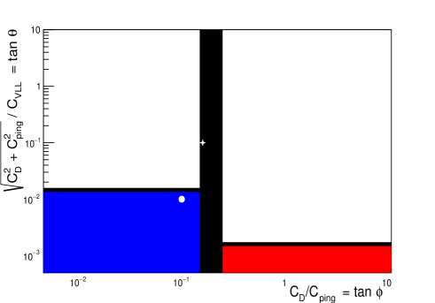
Figure 2: The white regions indicate ratios of operator coefficients that the type II seesaw cannot predict, as discussed after Eq. (2.8), where $\tan\theta$ and $\tan\phi$ are defined. Upcoming experiments are sensitive to the plotted ranges of the ratios. These estimates are independent of the neutrino mass hierarchy and mass scale; the star and circle are located respectively in the regions predicted in NH and IH for $m_{min}=0$ and specific choices of the Majorana phase (but the regions can be larger when the phase varies; the IH region has filaments).

3 Inverse Type I seesaw

In this section, we consider the inverse type I seesaw model Wyler:1982dd ; Mohapatra:1986aw ; Mohapatra:1986bd , which generates neutrino masses via the exchange of heavy gauge-singlet fermions. Like the type II seesaw, the model can generate LFV without Lepton Number Violation, so LFV rates are not suppressed by small neutrino masses. However, unlike the type II case, the flavour-changing couplings are disconnected from the neutrino mass matrix, and several heavy new particles are added, with potentially different masses.

We add to the SM $n$ pairs of gauge singlet fermions $N,S$ of opposite chirality, with the interactions

$$\delta\mathcal{L}_{NS}=i\overline{N}\not{\partial}N+i\overline{S}\not{\partial}S-\left(Y^{\alpha a}_{\nu}(\overline{\ell}_{\alpha}\tilde{H}N_{a})+M_{ab}\overline{S}_{a}N_{b}+\frac{1}{2}\mu_{ab}\overline{S_{a}}S^{c}_{b}+{\rm h.c}\right),$$ (3.1)

where $Y_{\nu}$ is a complex $3\times n$ dimensionless matrix and $M,\mu$ are $n\times n$ mass matrices. If Lepton Number is attributed to $\ell,N$ and $S$, then only $\mu$ is Lepton Number Violating. Upon the spontaneous breaking of the electroweak symmetry, the neutrino mass Lagrangian reads (suppressing flavour indices)

$$\mathcal{M}_{\nu N}=\overline{\begin{pmatrix}\nu_{L}&N^{c}&S\end{pmatrix}}\begin{pmatrix}0&m_{D}&0\\ m_{D}^{T}&0&M^{T}\\ 0&M&\mu\end{pmatrix}\begin{pmatrix}\nu^{c}_{L}\\ N\\ S^{c}\end{pmatrix}+{\rm h.c.}$$ (3.2)

which, in the seesaw limit ($Y_{\nu}v=m_{D}\ll M$), give the following active neutrino masses

$$m_{\nu}=m_{D}(M^{-1})\mu(M^{T})^{-1}m^{T}_{D}.$$ (3.3)

while for $M\gg\mu$ the $N,S$ pairs have pseudo-Dirac masses determined by the eigenvalues of $M$. Neutrino masses and oscillation parameters can be obtained by adjusting the lepton number breaking matrix $\mu$ for arbitrary choices of the Yukawa couplings $Y_{\nu}$ and sterile neutrino masses $M$. This contrasts with the “vanilla” type I seesaw expectation of GUT scale sterile neutrinos or suppressed Yukawa couplings Minkowski:1977sc ; Gell-Mann:1979vob ; Yanagida:1979as ; Glashow:1979nm ; Mohapatra:1979ia , which give negligible contributions to LFV observables.

In the following, we consider $M\sim$ TeV and allow $Y_{\nu}$ to vary in the parameter space allowed by current LFV searches and other experimental constraints. Low-scale type I seesaw models can be directly probed via the production of the heavy neutral leptons at colliders delAguila:2007qnc ; Atre:2009rg ; Deppisch:2015qwa ; Banerjee:2015gca ; Antusch:2016vyf ; Das:2018usr ; Mekala:2022cmm , or indirectly through the active-sterile neutrino mixing (or the associated non-unitarity of the effective $3\times 3$ lepton mixing matrix), which affect electroweak precision observables, universality ratios and lepton flavor violating processes Antusch:2014woa ; Fernandez-Martinez:2016lgt ; Chrzaszcz:2019inj ; Blennow:2023mqx .

3.1 $\mu\to e$ LFV

(a) $\mathcal{O}(Y_{\nu}Y^{\dagger}_{\nu})$ $Z,\gamma$ penguin diagram contributing to $\mu\to e$ four-vector operators.

(b) Penguin diagram proportional to four neutrino Yukawas contributing to the $\mu\to e$ four-fermion operators

(c) Box diagrams matching onto the $\mu\to e_{L}\overline{e_{L}}e_{L}$ vector

(d) Matching onto the $\mu\to e$ dipole operator

Figure 3: Matching contributions to $\mu\to e$ operators in the inverse seesaw. The diagrams illustrate the relevant interactions that are generated, but other diagrams may also contribute to the same operators 

Large lepton flavour violating transitions are among the distinctive features of the inverse seesaw Tommasini:1995ii ; Ilakovac:1994kj ; Ibarra:2011xn ; Dinh:2012bp ; Alonso:2012ji ; Abada:2015oba ; Coy:2018bxr ; Abada:2021zcm ; Zhang:2021jdf ; Coy:2021hyr ; Granelli:2022eru ; Crivellin:2022cve . In this paper, we focus on the contact interactions that are relevant for $\mu\to e$ observables and aim at determining the region of the EFT coefficient space that the model cannot reach.

The LFV transitions we are interested in occurs in this model via loops, as we illustrate in Fig. 3. The four-fermion operator coefficients are obtained in matching out the heavy singlets in penguin and box diagrams. The vector four-fermion coefficients $C^{e\mu ff}_{V,LX}$, receive contributions from penguin diagrams shown in Figs. 3(a) and 3(b), which are respectively ${\cal O}(Y_{\nu}Y_{\nu}^{\dagger})$ and ${\cal O}(Y_{\nu}Y_{\nu}^{\dagger}Y_{\nu}Y_{\nu}^{\dagger})$. We include the diagram in Fig. 3(b) following Ref. Crivellin:2022cve , who observed that the contributions $\propto Y^{4}_{\nu}$ could be relevant for $Y_{\nu}$ $\mathcal{O}(1)$. The box diagrams of Fig. 3(c) also match onto vector four-lepton operators, while the diagrams of Fig. (3(d)) match onto the $\mu\to e$ dipole. Similarly to the type II seesaw model of Section 2, the new states couple to the left-handed doublets, so the operators featuring LFV currents with electron singlets are suppressed by the electron Yukawa coupling. As a result, the model matches onto five of the operators in Eq. (1.1). Leaving aside the one associated with $\mu\to e$ conversion on heavy nuclei, since upcoming experiments will use light targets, we are left with the following four coefficients:

$$C^{e\mu ee}_{V,LR} \simeq v^{2}\frac{\alpha_{e}}{4\pi}\bigg{(}1.5[Y_{\nu}M_{a}^{-2}\left(\frac{11}{6}+\ln\left(\frac{m^{2}_{W}}{M_{a}^{2}}\right)\right)Y_{\nu}^{\dagger}]_{e\mu}-2.7[Y_{\nu}(Y^{\dagger}_{\nu}Y_{\nu})_{ab}\frac{1}{M^{2}_{a}-M^{2}_{b}}\ln\left(\frac{M^{2}_{a}}{M^{2}_{b}}\right)Y_{\nu}^{\dagger}]_{e\mu}$$

$$+ \mathcal{O}\left(\frac{\alpha_{e}}{4\pi}\right)\bigg{)}$$

$$C^{e\mu}_{Alight,L} \simeq v^{2}\frac{\alpha_{e}}{4\pi}\bigg{(}-0.6[Y_{\nu}M_{a}^{-2}\left(\frac{11}{6}+\ln\left(\frac{m^{2}_{W}}{M_{a}^{2}}\right)\right)Y_{\nu}^{\dagger}]_{e\mu}+1.1[Y_{\nu}(Y^{\dagger}_{\nu}Y_{\nu})_{ab}\frac{1}{M^{2}_{a}-M^{2}_{b}}\ln\left(\frac{M^{2}_{a}}{M^{2}_{b}}\right)Y_{\nu}^{\dagger}]_{e\mu}$$

$$+ \mathcal{O}\left(\frac{\alpha_{e}}{4\pi}\right)\bigg{)}$$

$$C^{e\mu ee}_{V,LL} \simeq v^{2}\frac{\alpha_{e}}{4\pi}\bigg{(}-1.8[Y_{\nu}M_{a}^{-2}\left(\frac{11}{6}+\ln\left(\frac{m^{2}_{W}}{M_{a}^{2}}\right)\right)Y_{\nu}^{\dagger}]_{e\mu}+2.7[Y_{\nu}(Y^{\dagger}_{\nu}Y_{\nu})_{ab}\frac{1}{M^{2}_{a}-M^{2}_{b}}\ln\left(\frac{M^{2}_{a}}{M^{2}_{b}}\right)Y_{\nu}^{\dagger}]_{e\mu}$$

$$+ 2.5Y^{ea}_{\nu}Y^{*\mu a}_{\nu}Y^{eb}_{\nu}Y^{*eb}_{\nu}\frac{1}{M^{2}_{a}-M^{2}_{b}}\ln\left(\frac{M^{2}_{a}}{M^{2}_{b}}\right)+\mathcal{O}\left(\frac{\alpha_{e}}{4\pi}\right)\bigg{)}$$

$$C^{e\mu}_{D,R} \simeq -\frac{v^{2}}{2}\left(\frac{\alpha_{e}}{4\pi e}\right)[Y_{\nu}M^{-2}Y_{\nu}^{\dagger}]_{e\mu},$$ (3.4)

where $a,b$ are summed over the number $n$ of sterile neutrinos. We include the finite part of the penguin diagrams shown in Fig. 3(a) because the ratios of sterile masses and the electroweak scale involved in the logarithms are not large (as we discuss in the introduction). Higher-order terms in the $\alpha_{e}/(4\pi)$ expansion are neglected because they are small and would require including some two-loop diagrams for a consistent treatment. Consequently, the results presented in Eq. (3.4) are reliable at the $\lesssim 10\%$ level.

The above coefficients, generated by the model and in principle observable, are linear combinations of four contractions of the Yukawa and sterile neutrino mass matrices (which we refer to as “invariants”). Since the number of coefficients equals the number of invariants, it seems that the model could predict any observation – i.e. any point in the 4-dimensional space of the operator coefficients – with suitable choices of the $Y_{\nu}$ and $M$ matrices. However, the number of invariants is reduced if the sterile neutrinos are nearly degenerate . In this limit, the combination entering the $\mathcal{O}(Y_{\nu}Y^{\dagger}_{\nu})$ penguin contributions aligns with the matrix elements parameterizing the dipole coefficient. Indeed, by expanding $M^{2}_{a}/M^{2}=1+x_{a}$ for small $x_{a}$ (where $M$ now denotes the average sterile neutrino mass), we have that

$$\frac{1}{M_{a}^{2}}\left(\frac{11}{6}+\ln\left(\frac{m_{W}^{2}}{M^{2}_{a}}\right)\right) =\frac{1}{M^{2}(1+x_{a})}\left(\frac{11}{6}+\ln\left(\frac{m_{W}^{2}}{M^{2}}\right)-\ln(1+x_{a})\right)$$

$$=\frac{1}{M^{2}}\left(\frac{11}{6}+\ln\left(\frac{m_{W}^{2}}{M^{2}}\right)+\mathcal{O}(x_{a})\right).$$ (3.5)

If the mass-splitting between the heavy singlets is $\lesssim v^{2}$, the error introduced by the degenerate approximation is a dimension eight $v^{2}/M^{2}$ suppressed contribution, that, for TeV scale sterile masses, would be approximately of the same order of the neglected $\mathcal{O}(\alpha_{e}/4\pi)$ corrections. Similarly, the leading order term in the $x_{a}$ expansion of the mass function that enters in the $\mathcal{O}(Y_{\nu}Y_{\nu}^{\dagger}Y_{\nu}Y_{\nu}^{\dagger})$ penguin and in the boxes is

$$\frac{1}{M^{2}_{a}-M^{2}_{b}}\ln\left(\frac{M^{2}_{a}}{M^{2}_{b}}\right)=\frac{1}{M^{2}}\left(1+\mathcal{O}(x_{a},x_{b})\right),$$ (3.6)

so that in the nearly degenerate limit, we find

$$C^{e\mu}_{D,R}(m_{\mu}) \simeq-10^{-3}\frac{v^{2}}{M^{2}}(Y_{\nu}Y^{\dagger}_{\nu})_{e\mu}$$

$$C^{e\mu}_{Alight,L}(m_{\mu}) \simeq\frac{v^{2}}{M^{2}}\left(10^{-3}(Y_{\nu}Y^{\dagger}_{\nu})_{e\mu}+6.6\times 10^{-4}(Y_{\nu}Y^{\dagger}_{\nu}Y_{\nu}Y^{\dagger}_{\nu})_{e\mu}\right)$$

$$C^{e\mu ee}_{V,LR}(m_{\mu}) \simeq\frac{v^{2}}{M^{2}}\left(-2.8\times 10^{-3}(Y_{\nu}Y^{\dagger}_{\nu})_{e\mu}-1.6\times 10^{-3}(Y_{\nu}Y^{\dagger}_{\nu}Y_{\nu}Y^{\dagger}_{\nu})_{e\mu}\right)$$

$$C^{e\mu ee}_{V,LL}(m_{\mu}) \simeq\frac{v^{2}}{M^{2}}\left(3.3\times 10^{-3}(Y_{\nu}Y^{\dagger}_{\nu})_{e\mu}(1+0.56(Y_{\nu}Y^{\dagger}_{\nu})_{ee})+1.55\times 10^{-3}(Y_{\nu}Y^{\dagger}_{\nu}Y_{\nu}Y^{\dagger}_{\nu})_{e\mu}\right)$$ (3.7)

Despite the large number of free parameters in the inverse seesaw model, even in the degenerate limit, the coefficients of the $\mu\to e$ operators can now be determined by just two invariant contractions of the neutrino Yukawa matrix. Being linear combinations of two invariants, the correlations of the operator coefficients that the model can predict are restricted: by measuring two (complex) coefficients, it would be possible to predict the others. Focusing on the first three operators of Eq. (3.7), we find that

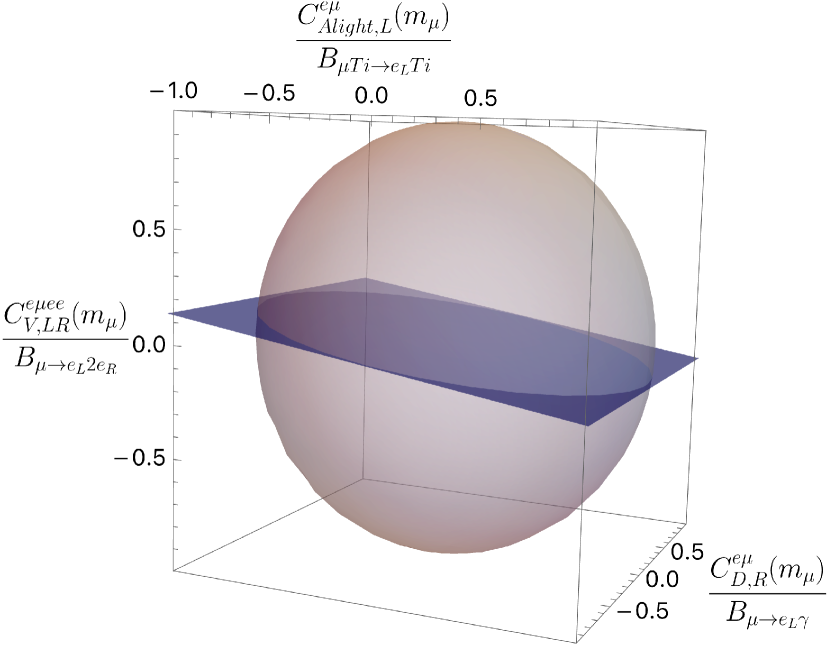
(a) The light-gray sphere illustrate the experimentally allowed ellipse in the $C^{e\mu}_{D,R}(m_{\mu}),C^{e\mu ee}_{Alight,L}(m_{\mu}),C^{e\mu ee}_{V,LR}(m_{\mu})$ space. We consider the real parts of the coefficients and normalise to the current upper bound. If the sterile neutrinos are nearly degenerate, the model can cover the region defined in Eq. (3.8), which correspond to the blue plane.

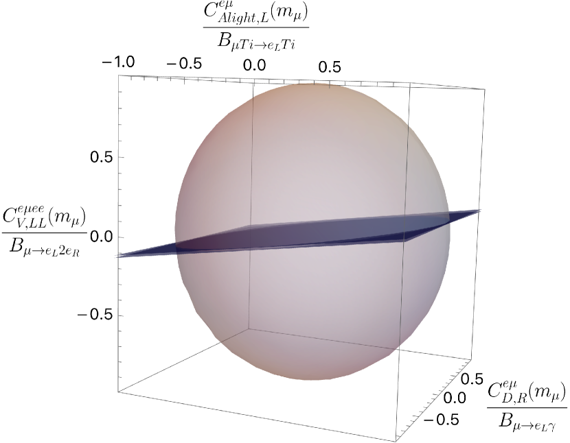
(b) The light-gray sphere illustrate the experimentally allowed ellipse in the $C^{e\mu}_{D,R}(m_{\mu}),C^{e\mu ee}_{Alight,L}(m_{\mu}),C^{e\mu ee}_{V,LL}(m_{\mu})$ space. We consider the real parts of the coefficients and normalise to the current upper bound. If the sterile neutrinos are nearly degenerate, the model can cover the region defined in Eq. (3.9) and correspond to the volume delimited by the two blue planes (see Fig. 4(c))

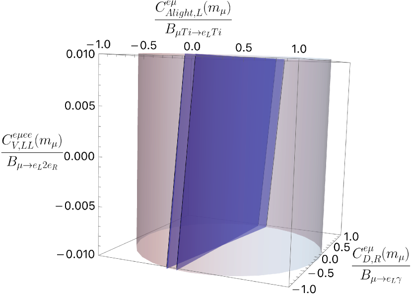
(c) Zoom of Fig. 4(b). The model can cover only the region enclosed by the two planes.

Figure 4: Parameter space covered by the inverse seesaw (with degenerate sterile neutrinos) in the low-energy operator coefficient space

$$C^{e\mu ee}_{V,LR}(m_{\mu})=-2.4C^{e\mu}_{Alight,L}(m_{\mu})+0.02C^{e\mu}_{D,R}(m_{\mu})$$ (3.8)

In the purely left-handed $\mu\to 3e$ vector the magnitude of the coefficient multiplying the matrix element $(Y_{\nu}Y^{\dagger}_{\nu})_{e\mu}$ is dependent on the real and positive parameter $(Y_{\nu}Y^{\dagger}_{\nu})_{ee}$ arising from the box diagram contribution. However, since the Yukawa couplings are assumed to be perturbative $(Y_{\nu}Y^{\dagger}_{\nu})_{ee}\lesssim 1$, we can similarly find that

$$C^{e\mu ee}_{V,LL}(m_{\mu})=2.4C^{e\mu}_{Alight,L}(m_{\mu})+c_{d}C^{e\mu}_{D,R}(m_{\mu})$$ (3.9)

where $-1.99\lesssim c_{d}\lesssim-0.57$. The correlations described by Eqs. (3.8) and (3.9) hold, within the accuracy of our calculations, for general complex coefficients. To visually represent the parameter space accessible to the inverse seesaw model, we consider the real parts of the coefficients and plot the corresponding planes in the 3D space of low-energy coefficients. By normalizing each coefficient to the upper limit imposed by current experimental searches, the allowed region of parameter space correspond to the interior of a sphere. The inverse seesaw model (with nearly degenerate sterile neutrinos) can sit in the intersection of this region with the planes defined by Eq. (3.8) and Eq. (3.9), as illustrated in Fig. 4. Since the dipole coefficient in Eq. (3.9) is unknown but bounded, the model can cover the volume enclosed by the two extreme planes

4 Leptoquark

This section studies the $\mu\!\to\!e$ predictions of an SU(2) singlet leptoquark of hypercharge $Y=1/3$ that could fit the the R_D anomaly BaBar:2012obs ; Belle:2015qfa ; Belle:2019rba ; LHCb:2023zxo ; LHCb:2023cjr ; Sakaki:2013bfa ; Cai:2017wry ; Angelescu:2018tyl ; Lee:2021jdr , which is an excess of $b\to c\bar{\tau}\nu$ events. Requiring the leptoquark to fit $R_{D}$ fixes the mass to be O(TeV) and restricts the quantum numbers, but our $\mu\!\to\!e$ interactions are independent of the couplings that contribute to $R_{D}$. Unlike the models of the previous sections, the leptoquark couples to both lepton doublets and singlets, and can mediate $\mu A\to\!eA$ at tree level – but does not generate neutrino masses.

The SU(2)-singlet leptoquark is denoted $S_{1}$ Buchmuller:1986zs (not to be confused with the singlet fermions $\{S_{a}\}$ of the previous section), with interactions:

$${\cal L}_{S} = (D_{\rho}S_{1})^{\dagger}D^{\rho}S_{1}-m_{LQ}^{2}S_{1}^{\dagger}S_{1}+(-\lambda^{\alpha j}_{L}\overline{\ell}_{\alpha}i\tau_{2}q_{j}^{c}+\lambda^{\alpha j}_{R}\overline{e}_{\alpha}u_{j}^{c})S_{1}+(\lambda^{\alpha j*}_{L}\overline{q^{c}}_{j}i\tau_{2}\ell_{\alpha}+\lambda^{\alpha j*}_{R}\overline{u^{c}}_{j}e_{\alpha})S_{1}^{\dagger}$$

$$+{\rm~{}Higgs~{}interactions}$$

where the leptoquark mass is $m_{LQ}\simeq$ TeV, the generation indices are $\alpha\in\{e,\mu,\tau\}$ and $j\in\{u,c,t\}$, and the sign of the doublet contraction is taken to give $+\lambda^{\alpha j}_{L}\overline{e_{L}}(u_{L})^{c}S_{1}$. Like in the type II model of Section 2, the leptoquark-Higgs interactions are neglected because their contributions to LFV observables are negligible assuming perturbative couplings.

Leptoquarks are strongly interacting, so can be readily produced at hadron colliders; the current LHC searches impose $m_{LQ}\mathrel{\vbox{\hbox{$>$}\nointerlineskip\hbox{$\sim$}}}$ 1-2 TeV ParticleDataGroup:2022pth . Also, their peculiar Yukawa interactions connecting quarks to leptons, can predict diverse quark and/or lepton flavour-changing processes Crivellin:2020mjs ; Lee:2021jdr ; Coy:2021hyr . For instance, non-zero $\lambda^{\mu u}_{X}$, $\lambda^{\mu c}_{X},\lambda^{eu}_{X}$ and $\lambda^{ec}_{X}$ induce $\mu\to e$ processes on a $u$ and $c$ quark currents – which we study here – and also induce LFV $D$ decays with $e^{\pm}\mu^{\mp}$ in the final state. In addition, $S_{1}$ will mediate $\Delta F=2$ four-quark operators via box diagrams which can contribute to meson-anti-meson mixing UTfit:2007eik . We did not find relevant constraints on the LFV interactions of $S_{1}$ from quark flavour physics, but will discuss in more detail the complementarity of quark and lepton observables in pl2 .

In matching the leptoquark onto the QCD$\times$QED-invariant EFT at $m_{LQ}$, vector ($\propto\lambda^{*}_{R}\lambda_{R}$, $\lambda^{*}_{L}\lambda_{L}$), and scalar/tensor ($\propto\lambda^{*}_{R}\lambda_{L}$, $\lambda^{*}_{L}\lambda_{R}$) operators are generated at tree-level. We only consider the subset which are quark flavour-diagonal and $\mu\!\to\!e$ flavour-changing. The model matches onto vector four-fermion operators of the form $(\bar{e}\gamma^{\rho}P_{X}\mu)(\bar{f}\gamma_{\rho}P_{Y}f)$ (where $X,Y\in\{L,R\}$ and $f$ any lepton or quark) via “penguin” diagrams (see Fig. 5(a)), and also can generate vector four lepton operators via box diagrams as in Fig. 5(b). Finally, the dipole operators can be generated via the last diagram of Fig. 5. This collection of operators at the leptoquark mass scale is schematically represented in Fig. 6 as the top row of boxes and ovals.

(a) Penguin diagram contributing to the $\mu\to e$ four-fermion operators.

(b) Example box diagram matching onto the $\mu\to e_{L}\overline{e_{L}}e_{L}$ vector

.

(c) Illustrative contribution matching to the dipole operator.

Figure 5: Representative diagrams for the matching of the leptoquark onto four-fermion operators, and the dipole. 

Several of the operators generated in matching out the leptoquark are present in the Lagrangian of Eq. (1.1). For instance, $S_{1}$ matches onto vector and/or scalar $\bar{e}$-$\mu$-$\bar{u}$-$u$ operators, which give large contributions to $\mu A\to\!eA$. In addition, the log-enhanced loops change the predictions significantly: the coefficients of scalar and tensor quark operators respectively grow and shrink due to QCD, and QED loops can cause some ${\cal O}(1)$ mixing, such as the top and charm tensors into the dipole, or the $u$-tensor into the $u$-scalar. The effect of the RGEs is represented by lines in Fig. 6.

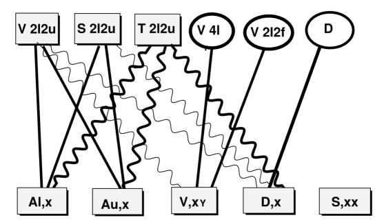
Figure 6: A schematic representation of how the leptoquark generates $\mu\to e\gamma$, $\mu\to e\bar{e}e$ and $\mu A\to\!eA$. The top row represents classes of coefficients, generated in matching out the leptoquark, of given Lorentz structure and particle type, for any flavours and chiralities. The boxes correspond to operators with coefficients of ${\cal O}(\lambda^{2}/m_{LQ}^{2})$, whereas the ovals have suppressed coefficients $\sim{\cal O}(\lambda^{2}/[16\pi^{2}m_{LQ}^{2}])$, or $\sim{\cal O}(\lambda^{4}/[16\pi^{2}m_{LQ}^{2}])$. The bottom row of boxes are the six observable coefficients (for fixed $e$ chirality in the $\mu\!\to\!e$ bilinear) of Eq. (1.1). Lines represent the transformation between the $m_{LQ}$ and experimental scale; a straight line means the observable coefficient can be directly obtained in matching. Operator mixing is represented as wavy lines: a thick line indicates an ${\cal O}(1)$ contribution of at least one operator from the class to the observable; a thin line indicates a more suppressed ${\cal O}(\alpha)$ contribution.

At the experimental scale, the $S_{1}$ leptoquark generates both $\mu\to e_{L}$ and $\mu\to e_{R}$ coefficients. For conciseness, we give results for $\mu\to e_{L}$; the $\mu\to e_{R}$ coefficients can be obtained by judiciously interchanging $R\leftrightarrow L$. The contribution to the dipole coefficients is

$$\frac{m_{LQ}^{2}}{v^{2}}C^{e\mu}_{D,R}(m_{\mu}) \simeq \frac{e[\lambda_{L}\lambda^{\dagger}_{L}]^{e\mu}}{128\pi^{2}}\left(1-16\frac{\alpha_{e}}{4\pi}\ln\frac{m_{LQ}}{m_{\mu}}\right)+\frac{2\alpha^{2}_{e}}{9\pi^{2}e}\left[\lambda_{L}\ln\frac{m_{LQ}}{m_{Q}}\lambda^{\dagger}_{L}\right]^{e\mu}$$ (4.1)

$$-\frac{\alpha_{e}}{2\pi ey_{\mu}}\left[\lambda_{L}Y_{u}\tilde{f}^{Q}\ln\frac{m_{LQ}}{m_{Q}}\lambda^{\dagger}_{R}\right]^{e\mu}~{}~{}~{}~{}~{}~{}~{}~{}~{}~{}~{}~{}~{}$$

where the first term is the matching contribution (times its QED running), the second term is the 2-loop mixing of tree vector operators into the dipole, the last term is the RG-mixing of tensor operators to dipoles, and the $m_{Q}$ serving as lower cutoff for the logarithms (here and further in the paper) is max$\{m_{Q},2~{}{\rm GeV}\}$ . For $C^{e\mu}_{D,L}$, one interchanges $R\leftrightarrow L$. The QCD running of the quark tensor operator is intricated with the QED mixing to the dipole Bellucci:1981bs ; Buchalla:1989we , so induces a quark-flavour-dependent rescaling $\tilde{f}^{Q}\simeq\{1,1.4\}$ for $\{t,c\}$ quarks.

The leptoquark also generates vector four-lepton operators (for $X\in\{L,R\}$)

$$\frac{m_{LQ}^{2}}{v^{2}}C_{V,LX}^{e\mu ee}(m_{\mu}) \simeq -\frac{N_{c}}{64\pi^{2}}[\lambda_{L}\lambda_{L}^{\dagger}]^{e\mu}[\lambda_{X}\lambda_{X}^{\dagger}]^{ee}\left(1\mp 12\frac{\alpha_{e}}{4\pi}\ln\frac{m_{LQ}}{m_{\mu}}\right){+}\frac{\alpha_{e}}{3\pi}\left[\lambda_{L}\ln\frac{m_{LQ}}{m_{Q}}\lambda_{L}^{\dagger}\right]^{e\mu}$$ (4.2)

$$-g^{e}_{X}\frac{N_{c}}{16\pi^{2}}\left[\lambda_{L}Y_{u}\ln\frac{m_{LQ}}{m_{Q}}Y_{u}^{\dagger}\lambda^{\dagger}_{L}\right]^{e\mu}$$

where $g^{e}_{L}=-1+2\sin^{2}\theta_{W}$, $g^{e}_{R}=2\sin^{2}\theta_{W}$, the first term represents the box diagram at $m_{LQ}$ (and its QED running to $m_{\mu}$, with $-$/$+$ for X=/$\neq$Y) which is represented as the $V,4l$ oval at the top of Fig. 6 connecting to the $V_{XY}$ box at the bottom, the second term is the log-enhanced photon penguin that mixes the tree operators ${\cal O}_{VLL}^{QQ}$ (for $Q\in\{u,c,t\}$) into 4-lepton operators (represented in Fig. 6 as a thin wavy line between the $V,2l2u$ and $V_{XY}$ boxes), and the last term is the contribution of the $Z$-penguins shown in Fig. 5(a) (the $V2l2f$ oval of Fig. 6), not including the negligible effect of the RGEs.

The scalar 4-lepton coefficient $C_{SXX}^{e\mu ee}$ can be generated via a box diagram, with Higgs insertions on the internal quark lines (so the coefficient can be significant for internal top quarks); however, the coupling constant combination that appears on the flavour-changing line is already strictly constrained by $\mu\to e\gamma$. So this coefficient has a very small contribution to $\mu\to e$ processes, and we neglect it.

A classic signature of leptoquarks is $\mu A\to\!eA$, which can be mediated at tree level via scalar or vector operators involving first generation quarks. The constraint from light targets like Titanium or Aluminium can be written (for outgoing $e_{L}$)

$$\sqrt{\frac{BR^{exp}_{Ti}}{250}} \mathrel{\vbox{\hbox{$>$}\nointerlineskip\hbox{$\sim$}}} {\Big{|}}0.250C_{D,R}(m_{\mu})+0.37\lambda^{eu}_{L}\lambda^{\mu u*}_{L}.\left(1{+}\frac{{2}\alpha}{\pi}\ln\right)+0.39\left(\frac{g^{2}}{64\pi^{2}}\lambda^{eu}_{L}\lambda^{\mu u*}_{L}\ln\frac{m_{LQ}}{m_{W}}\right)$$

$$-\frac{\alpha}{6\pi}\left[\lambda_{L}\ln\frac{m_{LQ}}{m_{Q}}\lambda^{\dagger}_{L}\right]^{e\mu}{-\frac{3}{{64}\pi^{2}}\left[\lambda_{L}Y_{u}\ln\frac{m_{LQ}}{m_{Q}}Y_{u}^{\dagger}\lambda^{\dagger}_{L}\right]^{e\mu}}$$

$$-\eta\left(1.95\lambda^{eu}_{L}\lambda^{\mu u*}_{R}+\frac{0.41m_{N}}{27m_{c}}\lambda^{ec}_{L}\lambda^{\mu c*}_{R}\right)+\eta(m_{t})\frac{1.07m_{N}}{27m_{t}}\lambda^{et}_{L}\lambda^{\mu t*}_{R}{\Big{|}}\times\frac{v^{2}}{m_{LQ}^{2}}\ ,$$

where in order, the terms are: the dipole coefficient given in Eq. (4.1), the tree vector coefficient on $u$ quarks with its QED running (represented as the upper left box of Fig. 6), the electroweak box contribution to the $d$ vector, the QED then $Z$ penguin (see Fig. 5(a)) contributions to the $u$ and $d$ vectors (where we took $V_{ud}=1,\sin^{2}\theta_{W}=1/4$), and the scalar $u$, $c$ and $t$ contributions. Most of the scalar top contribution comes from a loop-induced flavour changing Higgs coupling (in SMEFT, ${\cal O}^{e\mu tt}_{LEQU}$ mixing into ${\cal O}^{e\mu}_{EH}$), which generates scalar quark operators of all quark flavours. The tensor to scalar mixing is neglected, because the model generates tensor coefficients that are proportional to the scalars. The QCD and QED running of the scalars is contained in $\eta$:

$$\eta =\left[\frac{\alpha_{s}(m_{LQ})}{\alpha_{s}(2{\rm GeV})}\right]^{-12/23}\!\!\!\!\!\!\times(1+\frac{13\alpha}{6\pi}\ln\frac{m_{LQ}}{2{\rm GeV}})\approx 1.79,$$

$$\eta(m_{t}) =\left[\frac{\alpha_{s}(m_{LQ})}{\alpha_{s}(m_{t})}\right]^{-12/23}\!\!\!\!\!\!\times(1+\frac{13\alpha}{6\pi}\ln\frac{m_{LQ}}{m_{t}})\approx 1.11.$$ (4.4)

It is easy to see that the operator coefficients of Eq. (1.1) depend on more than 12 different combinations of the leptoquark couplings, so the only prediction of the leptoquark model is that the four-lepton scalar coefficients $C_{S,XX}^{e\mu ee}$ are negligible, as discussed after Eq. (4.2); the model could fit any observed values for the remaining 10 coefficients.

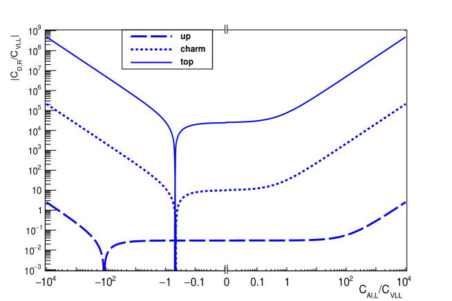
Figure 7: The $S_{1}$ leptoquark interacting only with one quark generation predicts relations among coefficients given in Appendix C: for large positive values of the four-fermion coefficient on light targets $C_{Alight,L}^{e\mu}/C_{V,LL}^{e\mu ee}$ (horizontal,in log), the ratio $C_{DR}^{e\mu}/C_{V,LL}^{e\mu ee}$ (magnitude on the vertical) is large and positive. The four-lepton coefficients are comparable for all quark generations.

However, the leptoquark has the interesting feature of predicting specific patterns of $\mu\!\to\!e$ LFV when this occurs with only one quark generation: in this case, all the four-lepton coefficients are of comparable magnitude, and knowing in addition the dipole allows to predict $C_{AL,X}$ (or vice versa). To illustrate this, we neglect the box contributions to 4-lepton operators (discussed in more detail in pl2 ), which are subdominant for internal $t$ quarks, but can give an ${\cal O}(1)$, same-sign contribution for internal $u$ and $c$ quarks when $\lambda_{X}^{eQ}\sim 1$. Without the boxes, all the coefficients are determined by four combinations of coupling constants: $\lambda^{eQ}_{X}\lambda^{\mu Q*}_{X}$ and $\lambda^{eQ}_{X}\lambda^{\mu Q*}_{Y}$ for $X,Y\in\{L,R\}$ and $Y\neq X$ (the expressions for the coefficients are given in Appendix C). This leads to correlations among operator coefficients, as occurred in the inverse seesaw. In Fig. 7, we illustrate this correlation by plotting ratios of coefficients, rather than the 3-$d$ plots of Section 3 (notice that the horizontal axis is in log₁₀ scale, but runs from negative to positive values, so small values of $C_{Al,X}$ have been deleted at the origin).

One sees that “generically”, a leptoquark coupled to the $t$ gives a large dipole, whereas a large $\mu A\to\!eA$ rate is expected for leptoquarks interacting with the up quark. However, neither of these expectations is an unambiguous footprint of the quark flavour dominantly coupled to the leptoquark, because $C_{Al,X}$ (resp. $C_{D,X}$) can vanish for leptoquarks interacting with $u$ (resp. $t$) quarks. Therefore, the observation of $\mu\to 3e$ without $\mu\to e\gamma$ would not exclude an $S_{1}$ leptoquark coupling mostly to top quarks; it would just exclude generic values of the parameters of that model (i.e., values of the parameters that do not lead to cancellation in some Wilson coefficients). Similarly, the observation of $\mu\to e\gamma$ but not $\mu\to e$ conversion on light nuclei would not exclude an $S_{1}$ leptoquark coupling only to up quarks.

5 Discussion and Summary

In this paper, we explored whether a bottom-up EFT analysis (outlined in Section 1) can give a perspective on LFV models that is complementary to top-down studies. We emphasize that in EFT, the data for $\mu\to e\gamma$, $\mu\to e\bar{e}e$ and $\mu A\to\!eA$ consists of twelve Wilson coefficients, given in Eq. (1.1), and not just three branching ratios. The current experimental null-results confine the coefficients to the interior of a 12-D ellipse centered at the origin, and the aim of this paper was to determine whether a future observation could exclude models. To address this question, we searched for the regions of coefficient space accessible-to-future-experiments that each model cannot reach, as an observation in that part of the ellipse would rule the model out.

We studied three TeV-scale models: the type II seesaw, the inverse type I seesaw and a singlet scalar leptoquark added to the SM. We chose the first two because they can explain neutrino masses (which are the best motivation for LFV), while we considered the scalar leptoquark in light of the charged current anomaly observed in $b\to cl\nu$ transitions. The model predictions depend on combinations of NP and SM parameters which we refer to as “invariants”, see e.g. Eqs. (3.4) and (3.7).

The type II and inverse seesaw models generate Majorana neutrino masses via the tree-level exchange of heavy new particles, respectively a scalar triplet and fermion singlets. Large lepton-flavour-changing rates are possible because the models can contain LFV without lepton number violation, avoiding any suppression by small neutrino masses. In both models the new particles interact with lepton doublets, so the coefficients of operators with flavour-changing currents involving singlet charged leptons are suppressed by the lepton Yukawa couplings and neglected here:

$$C_{D,L}\,,\,C^{e\mu ee}_{V,RR}\,,\,C^{e\mu ee}_{V,RL}\,,\,C^{e\mu ee}_{S,RR}\,,\,C^{e\mu}_{Alight,R}\,,\,C^{e\mu}_{Aheavy,R}\,,\,C^{e\mu ee}_{S,LL}\,\simeq\,0~{}~{}~{}~{}{\rm(type~{}II,~{}inverse~{}seesaw)}$$

So in the twelve-dimensional space that can be probed by experiment, these models can only occupy 5 dimensions: should one of the above coefficients be observed (in the absence of the unsuppressed ones), then these models would be excluded. In addition, these vanishing coefficients imply that $\mu A\to\!eA$ only occurs via the dipole and vector interactions.

Section 2 showed that in the type II model, three of the remaining coefficients, $C^{e\mu}_{Alight,L}$, $C^{e\mu}_{Aheavy,L}$ and $C^{e\mu ee}_{V,LR}$ (given in Eqs. 2.4, 2.5) arise from the same loop diagrams and are all proportional to the same combination of invariants. This implies that the model occupies a line in the three-dimensional space of these three coefficients, and that one of the three rates for $\mu\to e_{L}\gamma$, $\mu\to e_{L}\bar{e}_{R}e_{R}$ and $\mu A\to e_{L}A$ being predicted by the other two. The coefficients $C^{e\mu}_{D,R}$ and $C^{e\mu ee}_{V,LL}$ can be expressed in terms of two other invariants, all of which are constructed with the Yukawa matrix of the triplet scalar. This is proportional to the neutrino mass matrix, so known, up to the overall magnitude, the neutrino mass hierarchy, the lightest mass $m_{\rm min}$ and the Majorana Phases $\alpha_{1,2}$. So although the model generates $C^{e\mu ee}_{V,LL}$ at tree level, suggesting $\mu\to e\bar{e}e$ to discover the type II seesaw, this coefficient can vanish (for specific values of the Majorana phases and a range of $m_{min}$), as could $C^{e\mu}_{D,R}$ or $C^{e\mu ee}_{V,LR}$. When this occurs, the ratio of the remaining two coefficients is restricted, so there are combinations of observations that the type II seesaw cannot predict. This is illustrated in Fig. 2, where coefficient ratios (that correspond to angular coordinates in the three remaining dimensions of the original ellipse) are varied over the ranges accessible to upcoming experiments. We find that at least one of the four-fermion coefficients is always larger than the dipole, so that observing $\mu\to e\gamma$ with a branching ratio $Br(\mu\to e\gamma)\gtrsim 10^{-14}$ without detecting $\mu\to 3e$ in upcoming searches with $Br(\mu\to 3e)\gtrsim 10^{-16}$ can rule out the type II seesaw model studied here.

Section 3 studied the inverse seesaw model and showed that $C^{e\mu}_{D,R}$, $C^{e\mu ee}_{V,LL}$, $C^{e\mu ee}_{V,LR}$, $C^{e\mu}_{Alight,L}$ and $C^{e\mu}_{Aheavy,L}$ are functions of four invariants constructed from the neutrino Yukawa and sterile neutrino mass matrices, as given in Eq. (3.4). This implies that $Br(\mu Au\to e_{L}Au)$ could be predicted, given the rates for $\mu Al\to e_{L}Al$, $\mu\to e_{L}\bar{e}_{L}e_{L}$, $\mu\to e_{L}\bar{e}_{R}e_{R}$ and $\mu\to e_{L}\gamma$. The relevant contributions to these $\mu\to e$ coefficients arise via loop diagrams in matching (no four-SM-fermion operators are generated at tree-level), and are non-linear functions of the nondegenerate singlet masses. The RGEs of QED just renormalise these coefficients by a few percent, but do not generate additional invariants. So we observe that the number of invariants is reduced, if the sterile neutrino masses can be approximated as degenerate – as occurs for mass differences of $\mathcal{O}(v)$, see Eq. (3.5). In this limit, the five non-negligeable coefficients are controlled by two invariants constructed from the neutrino Yukawa matrices : $\mathcal{O}(Y_{\nu}Y_{\nu}^{\dagger})$ and $\mathcal{O}(Y_{\nu}Y_{\nu}^{\dagger}Y_{\nu}Y_{\nu}^{\dagger})$. This implies that when two coefficients are known, the remaining three are predicted, implying, eg, that the model predicts $Br(\mu A\to\!eA)$, from the rates for $\mu\to e\gamma$ and $\mu\to e\bar{e}e$. In the twelve-dimensional ellipse, our inverse seesaw model with degenerate sterile neutrinos therefore occupies a two-dimensional subspace (see Eqs. 3.8 and 3.9), which we illustrate in Fig. 4 by plotting the model prediction for the real part of three coefficients.

Finally, in Section 4, we investigated the $\mu\to e$ predictions of a singlet scalar leptoquark, selected to fit the excess of $b\to c\bar{\tau}\nu$ events observed in the $R_{D}$ ratio. The model contributes to all but two of the $\mu\to e$ observable coefficients with different coupling combinations, implying that it could entirely fill 10 dimensions of the 12-D ellipse. Only the observation of a non-zero $\mu\to 3e$ scalar coefficient $C^{e\mu ee}_{S,XX}$ could not be explained by the leptoquark. On the other hand, the model is more predictive when the leptoquark only interacts with one quark generation. In this case, all the invariants become $\propto\lambda_{X}^{eQ}\lambda_{L}^{\mu Q*}$ or $\lambda_{X}^{eQ}\lambda_{R}^{\mu Q*}$, so once four coefficients are measured, the remaining eight can be predicted. For a specific chirality of the outgoing electron in the LFV current, this resembles the degenerate inverse seesaw case, and the equations relating the coefficients are given in Appendix C. The relations between coefficient ratios that are expected when the leptoquark only interacts with one quark generation are illustrated in Fig. 7.

The results of this paper will be extended in a subsequent publication, where also some technical details of our EFT calculations will be discussed. We will explore the impact of complementary observables and the uses of invariants, and we will discuss the consequences of relative complex phases for the operator coefficients.

In summary, we find that there are observations of $\mu\to e$ processes that could rule out the three models we considered. The type II seesaw model predicts coefficients in part of a 3-dimensional subspace of the 12-d coefficient space accessible to experiments. The inverse seesaw maps onto a 4-d subspace of the 12-d space, in the case of non-dengenerate sterile neutrinos, but is more predictive for (nearly) degenerate steriles, where it is restricted to a 2-dimensional subspace. The singlet scalar leptoquark model does not generate sizable scalar four-lepton operators but can give arbitrary contributions to all other Wilson coefficients, thus completely filling 10 dimensions of the 12-d ellipse. However, if the leptoquark couplings to the electron and muon involve a single quark generation, the model predictions are restricted to a 4-dimensional subspace.

Acknowledgements

We thank Luca Silvestrini for a helpful suggestion, and Ann-Kathrin Perrevoort for helpful comments about observables in $\mu\to e\bar{e}e$. MA was supported by a doctoral fellowship from the IN2P3. The work of SL is supported in part by the European Union’s Horizon 2020 research and innovation programme under the Marie Sklodowska-Curie grant agreement No. 860881-HIDDeN.

Appendix A Appendix: Branching Ratios

For completeness, we list here the branching ratios for $\mu\to e\gamma$, and $\mu\to e\bar{e}e$:

$$BR(\mu\to e\gamma) = 384\pi^{2}(|C^{e\mu}_{DL}|^{2}+|C^{e\mu}_{DR}|^{2})~{}~{}~{},$$ (A.1)

$$BR(\mu\to e\bar{e}e) = \frac{|C^{e\mu ee}_{S,LL}|^{2}+|C^{e\mu ee}_{S,RR}|^{2}}{8}+(64\ln\frac{m_{\mu}}{m_{e}}-136)(|eC^{e\mu}_{D,R}|^{2}+|eC^{e\mu}_{D,L}|^{2})$$

$$+2|C^{e\mu ee}_{V,RR}+4eC^{e\mu}_{D,L}|^{2}+2|C^{e\mu ee}_{V,LL}+4eC^{e\mu}_{D,R}|^{2}$$

$$+|C^{e\mu ee}_{V,RL}+4eC^{e\mu}_{D,L}|^{2}+|C^{e\mu ee}_{V,LR}+4eC^{e\mu}_{D,R}|^{2}~{}~{}~{}.$$

Appendix B Appendix: the $\mu A\to\!eA$ operators

The Spin-Independent $\mu\to e$ conversion rate, normalised to the $\mu$ capture rate KKO ; Suzuki:1987jf can be written KKO

$${\rm BR}_{SI}(\mu A\to eA) = \frac{32G_{F}^{2}m_{\mu}^{5}}{\Gamma_{cap}}{\Big{[}}\big{|}\widetilde{C}^{pp}_{V,R}I_{A,V}^{(p)}+\widetilde{C}^{pp}_{S,L}I_{A,S}^{(p)}+\widetilde{C}^{nn}_{V,R}I_{A,V}^{(n)}+\widetilde{C}^{{}^{\prime}nn}_{S,L}I_{A,S}^{(n)}+C_{D,L}{\frac{I_{A,D}}{4}}\big{|}^{2}$$ (B.1)

$$+\{L\leftrightarrow R\}~{}{\Big{]}}~{}~{}~{},$$

where $I_{A,V}^{(N)}$, $I_{A,S}^{(N)}$ and $I_{A,D}$ are target($A$)-dependent “overlap integrals” inside the nucleus of the lepton wavefunctions and the appropriate nucleon density. This shows that a target probes a linear combination of coefficients identified by the overlap integrals. With current theoretical uncertainties on the overlap integrals, at least two independent combinations of the coefficients-on-nucleons $\{\tilde{C}\}$ could be constrained DKY . We will take these two combinations to correspond to light and heavy nuclei.

For light targets like Aluminium or Titanium, all the four-fermion overlap integrals are comparable, so the four-fermion operator that is probed is approximately

$$\mathcal{O}_{Alight,X}\approx\frac{1}{2}{\Big{(}}(\overline{e}P_{X}\mu)(\overline{p}p)+(\overline{e}\gamma^{\alpha}P_{X}\mu)(\overline{p}\gamma_{\alpha}p)+(\overline{e}P_{X}\mu)(\overline{n}n)+(\overline{e}\gamma^{\alpha}P_{X}\mu)(\overline{n}\gamma_{\alpha}n){\Big{)}}\hskip 14.22636pt$$ (B.2)

or more precisely, the KKO calculation says that the combination of coefficients probed by Aluminium is DKY

$$\tilde{C}_{Alight,X} = 0.455\widetilde{C}^{pp}_{S,X}+0.473\widetilde{C}^{pp}_{V,Y}+0.490\widetilde{C}^{nn}_{S,X}+0.508\widetilde{C}^{nn}_{V,Y})~{}~{}~{}.$$

For Gold, the coefficient combination is slightly misaligned:

$$\tilde{C}_{Aheavy,X} = 0.289\widetilde{C}^{pp}_{S,X}+0.458\widetilde{C}^{pp}_{V,Y}+0.432\widetilde{C}^{nn}_{S,X}+0.686\widetilde{C}^{nn}_{V,Y}~{}~{}~{},$$

indeed, the operator probed by heavy targets can be written as $\mathcal{O}_{Aheavy,X}=\cos\phi\mathcal{O}_{Alight,X}+\sin\phi\mathcal{O}_{Aheavy\perp,X}$. Measuring the coefficient of $\mathcal{O}_{Aheavy\perp,X}$ is the new information that can be obtained from heavy targets, but not light ones.

The definition of $\mathcal{O}_{Aheavy\perp,X}$ depends on whether it is constructed in the nucleon EFT, or the quark EFT relevant above a scale of 2 GeV. This is because there is information loss in matching nucleons to quarks, because the scalar densities of both $u$ and $d$ quarks in the neutron and proton are all comparable, so the scalar $u$ and $d$ coefficients $C_{SX}^{qq}$ are indistinguishable unless the scalar nucleon coefficients $\widetilde{C}^{NN}_{S,X}$ are accurately measured. In addition, there is a several-$\sigma$ discrepancy between the determinations of the scalar quark densities in the nucleon from the lattice and pion data.

So in this paper we focus on $\mu A\to\!eA$ on light targets, because only the leptoquark induces scalar quark coefficients, and we prefer to avoid the quark-scalar uncertainties associated with defining $\mathcal{O}_{Aheavy\perp,X}$ . We will consider the complementary information from heavy targets in pl2 .

Appendix C Appendix: If the leptoquark interacts only with one generation of quarks

In this appendix, we give formulae for the operator coefficients in the leptoquark model, for the case where the leptoquak interacts only with one generation of quarks.

If the leptoquark only interacts with top quarks, one obtains:

$$\frac{m_{LQ}^{2}}{v^{2}}C_{DR}(m_{\mu}) \simeq 2.3\times 10^{-4}[\lambda_{L}\lambda^{\dagger}_{L}]_{e\mu}-12[\lambda_{L}\lambda^{\dagger}_{R}]_{e\mu}$$ (C.1)

$$\frac{m_{LQ}^{2}}{v^{2}}C_{V,XY}^{e\mu ee}(m_{\mu}) \simeq -4.45\times 10^{-3}[\lambda_{X}\lambda_{X}^{\dagger}]_{e\mu}[\lambda_{Y}\lambda_{Y}^{\dagger}]_{ee}$$ (C.2)

$${+} (1.36\times 10^{-3}-g^{e}_{Y}0.033)[\lambda_{X}\lambda^{\dagger}_{X}]_{e\mu}$$

$$\frac{m_{LQ}^{2}}{v^{2}}C_{Alight,L} \simeq -6.8\times 10^{-4}\left[\lambda_{L}\lambda^{\dagger}_{L}\right]^{e\mu}-0.0084[\lambda_{L}\lambda^{\dagger}_{L}]^{e\mu}{+}2.4\times 10^{-4}\lambda^{et}_{L}\lambda^{\mu t*}_{R}$$

where $X,Y\in\{L,R\}$ for the vector four-lepton coefficients, for which the contributions due to boxes are included. The three terms of the four-fermion contribution to $\mu A\to\!eA$ are induced by the photon and $Z$ penguins, and the top-loop contribution to the $\mu\!\to\!e$ Yukawa coupling.

If the leptoquark only interacts with charm quarks, then:

$$\frac{m_{LQ}^{2}}{v^{2}}C_{DR}(m_{\mu}) \simeq 2.3\times 10^{-4}[\lambda_{L}\lambda^{\dagger}_{L}]_{e\mu}-0.42[\lambda_{L}\lambda^{\dagger}_{R}]_{e\mu}$$ (C.3)

$$\frac{m_{LQ}^{2}}{v^{2}}C_{V,XY}^{e\mu ee}(m_{\mu}) \simeq -4.5\times 10^{-3}[\lambda_{X}\lambda^{\dagger}_{X}]_{e\mu}[\lambda_{Y}\lambda_{Y}^{\dagger}]_{ee}{+}(4.8\times 10^{-3}-g^{e}_{Y}1.9\times 10^{-6})[\lambda_{X}\lambda^{\dagger}_{X}]_{e\mu}$$

$$\frac{m_{LQ}^{2}}{v^{2}}C_{Alight,L} \simeq -2.4\times 10^{-3}\left[\lambda_{L}\lambda^{\dagger}_{L}\right]^{e\mu}{-}0.02\lambda^{ec}_{L}\lambda^{\mu c*}_{R}$$

where $X,Y\in\{L,R\}$ in the vector four-lepton coefficients, for which the $Z$-penguin ( the last term) is suppressed $\propto m_{c}^{2}/v^{2}$, and any box can contribute because $(g-2)_{e}$ only constrains $\lambda^{ec}_{L}\lambda^{ec*}_{R}<0.7$.

And finally for a leptoquark that only has $\mu\!\to\!e$ interactions on $u$ quarks, one obtains:

$$\frac{m_{LQ}^{2}}{v^{2}}C_{DR}(m_{\mu}) \simeq 2.3\times 10^{-4}[\lambda_{L}\lambda^{\dagger}_{L}]_{e\mu}-7.3\times 10^{-4}[\lambda_{L}\lambda^{\dagger}_{R}]_{e\mu}$$ (C.4)

$$\frac{m_{LQ}^{2}}{v^{2}}C_{V,XY}^{e\mu ee}(m_{\mu}) \simeq -4.5\times 10^{-3}[\lambda_{X}\lambda^{\dagger}_{X}]_{e\mu}[\lambda_{Y}\lambda_{Y}^{\dagger}]_{ee}{+}4.8\times 10^{-3}[\lambda_{X}\lambda^{\dagger}_{X}]_{e\mu}$$

$$\frac{m_{LQ}^{2}}{v^{2}}C_{Alight,L} \simeq 0.38\lambda^{eu}_{L}\lambda^{\mu u*}_{L}-2.0\eta\lambda^{eu}_{L}\lambda^{\mu u*}_{R}$$ (C.5)

References

- (1) B. Abi et al. [Muon g-2], “Measurement of the Positive Muon Anomalous Magnetic Moment to 0.46 ppm,” Phys. Rev. Lett. 126 (2021) no.14, 141801 [arXiv:2104.03281 [hep-ex]].
- (2) J. P. Lees et al. [BaBar], “Evidence for an excess of decays,” Phys. Rev. Lett. 109 (2012), 101802 [arXiv:1205.5442 [hep-ex]].
- (3) M. Huschle et al. [Belle], “Measurement of the branching ratio of relative to decays with hadronic tagging at Belle,” Phys. Rev. D 92 (2015) no.7, 072014 [arXiv:1507.03233 [hep-ex]].
- (4) G. Caria et al. [Belle], “Measurement of and with a semileptonic tagging method,” Phys. Rev. Lett. 124 (2020) no.16, 161803 [arXiv:1910.05864 [hep-ex]].
- (5) [LHCb], “Measurement of the ratios of branching fractions and ,” arXiv:2302.02886 [hep-ex].
- (6) R. Aaij et al. [LHCb], “Test of lepton flavour universality using decays with hadronic channels,” [arXiv:2305.01463 [hep-ex]].
- (7) H. Georgi, “Effective field theory,” Ann. Rev. Nucl. Part. Sci. 43 (1993) 209-252; H. Georgi, “On-shell effective field theory,” Nucl. Phys. B361 (1991) 339-350.
- (8) A. J. Buras, “Weak Hamiltonian, CP violation and rare decays,” hep-ph/9806471.
- (9) Les Houches Lect. Notes 108 (2020): A. V. Manohar, “Introduction to Effective Field Theories,” [arXiv:1804.05863 [hep-ph]]; A. Pich, “Effective Field Theory with Nambu-Goldstone Modes,” [arXiv:1804.05664 [hep-ph]]; L. Silvestrini, “Effective Theories for Quark Flavour Physics,” [arXiv:1905.00798 [hep-ph]]; M. Balsiger, M. Bounakis, M. Drissi, J. Gargalionis, E. Gustafson, G. Jackson, M. Leak, C. Lepenik, S. Melville and D. Moreno, et al. “Solutions to Problems at Les Houches Summer School on EFT,” [arXiv:2005.08573 [hep-ph]].
- (10) S. Davidson, Y. Kuno and M. Yamanaka, “Selecting conversion targets to distinguish lepton flavour-changing operators,” Phys. Lett. B 790 (2019) 380 [arXiv:1810.01884 [hep-ph]].
- (11) A. M. Baldini et al. [MEG Collaboration], “Search for the lepton flavour violating decay with the full dataset of the MEG experiment,” Eur. Phys. J. C 76 (2016) no.8, 434 [arXiv:1605.05081 [hep-ex]].
- (12) A. M. Baldini et al. [MEG II Collaboration], “The design of the MEG II experiment,” Eur. Phys. J. C 78 (2018) no.5, 380 [arXiv:1801.04688 [physics.ins-det]];
- (13) U. Bellgardt et al. [SINDRUM Collaboration], “Search for the Decay mu+ -> e+ e+ e-,” Nucl. Phys. B 299 (1988) 1.
- (14) A. Blondel et al., “Research Proposal for an Experiment to Search for the Decay ,” arXiv:1301.6113 [physics.ins-det].
- (15) W. H. Bertl et al. [SINDRUM II Collaboration], “A Search for muon to electron conversion in muonic gold,” Eur. Phys. J. C 47 (2006) 337; C. Dohmen et al. [SINDRUM II Collaboration], “Test of lepton flavor conservation in mu -> e conversion on titanium,” Phys. Lett. B 317 (1993) 631.
- (16) Y. Kuno et al. (PRISM collaboration), ”An Experimental Search for a Conversion at Sensitivity of the Order of with a Highly Intense Muon Source: PRISM”, unpublished, J-PARC LOI, 2006.
- (17) M. Aoki et al. [C. Group], “A New Charged Lepton Flavor Violation Program at Fermilab,” [arXiv:2203.08278 [hep-ex]].
- (18) P. Wintz, “Results of the SINDRUM-II experiment,” Conf. Proc. C 980420 (1998), 534-546.
- (19) Y. G. Cui et al. [COMET Collaboration], “Conceptual design report for experimental search for lepton flavor violating mu- - e- conversion at sensitivity of 10**(-16) with a slow-extracted bunched proton beam (COMET),” KEK-2009-10; M. L. Wong [COMET Collaboration], “Overview of the COMET Phase-I experiment,” PoS FPCP 2015 (2015) 059.
- (20) R. M. Carey et al. [Mu2e Collaboration], “Proposal to search for with a single event sensitivity below ,” FERMILAB-PROPOSAL-0973.
- (21) B. Aubert et al. [BaBar], “Searches for Lepton Flavor Violation in the Decays tau+- — e+- gamma and tau+- — mu+- gamma,” Phys. Rev. Lett. 104 (2010), 021802 [arXiv:0908.2381 [hep-ex]].
- (22) Y. Miyazaki et al. [Belle], “Search for lepton flavor violating tau- decays into l- eta, l- eta-prime and l- pi0,” Phys. Lett. B 648 (2007), 341-350 [arXiv:hep-ex/0703009 [hep-ex]].
- (23) E. Kou et al. [Belle-II], “The Belle II Physics Book,” PTEP 2019 (2019) no.12, 123C01 [erratum: PTEP 2020 (2020) no.2, 029201] [arXiv:1808.10567 [hep-ex]].
- (24) J. Hisano, T. Moroi, K. Tobe and M. Yamaguchi, “Lepton flavor violation via right-handed neutrino Yukawa couplings in supersymmetric standard model,” Phys. Rev. D 53 (1996), 2442-2459 [arXiv:hep-ph/9510309 [hep-ph]].
- (25) S. Antusch, E. Arganda, M. J. Herrero and A. M. Teixeira, “Impact of theta(13) on lepton flavour violating processes within SUSY seesaw,” JHEP 11 (2006), 090 [arXiv:hep-ph/0607263 [hep-ph]].
- (26) A. Rossi, “Supersymmetric seesaw without singlet neutrinos: Neutrino masses and lepton flavor violation,” Phys. Rev. D 66 (2002), 075003 [arXiv:hep-ph/0207006 [hep-ph]].
- (27) W. Altmannshofer, A. J. Buras, S. Gori, P. Paradisi and D. M. Straub, “Anatomy and Phenomenology of FCNC and CPV Effects in SUSY Theories,” Nucl. Phys. B 830 (2010), 17-94 [arXiv:0909.1333 [hep-ph]].
- (28) V. Cirigliano, A. Kurylov, M. J. Ramsey-Musolf and P. Vogel, “Lepton flavor violation without supersymmetry,” Phys. Rev. D 70 (2004), 075007 [arXiv:hep-ph/0404233 [hep-ph]].
- (29) Y. Omura, E. Senaha and K. Tobe, “Lepton-flavor-violating Higgs decay and muon anomalous magnetic moment in a general two Higgs doublet model,” JHEP 05 (2015), 028 [arXiv:1502.07824 [hep-ph]].
- (30) E. Arganda, M. J. Herrero, X. Marcano and C. Weiland, “Imprints of massive inverse seesaw model neutrinos in lepton flavor violating Higgs boson decays,” Phys. Rev. D 91 (2015) no.1, 015001 [arXiv:1405.4300 [hep-ph]].
- (31) F. Deppisch and J. W. F. Valle, “Enhanced lepton flavor violation in the supersymmetric inverse seesaw model,” Phys. Rev. D 72 (2005), 036001 [arXiv:hep-ph/0406040 [hep-ph]].
- (32) K. Agashe, A. E. Blechman and F. Petriello, “Probing the Randall-Sundrum geometric origin of flavor with lepton flavor violation,” Phys. Rev. D 74 (2006), 053011 [arXiv:hep-ph/0606021 [hep-ph]].
- (33) M. Blanke, A. J. Buras, B. Duling, A. Poschenrieder and C. Tarantino, “Charged Lepton Flavour Violation and (g-2)(mu) in the Littlest Higgs Model with T-Parity: A Clear Distinction from Supersymmetry,” JHEP 05 (2007), 013 [arXiv:hep-ph/0702136 [hep-ph]].
- (34) T. M. Aliev, A. S. Cornell and N. Gaur, “Lepton flavour violation in unparticle physics,” Phys. Lett. B 657 (2007), 77-80 [arXiv:0705.1326 [hep-ph]].
- (35) Y. Cai, J. Herrero-García, M. A. Schmidt, A. Vicente and R. R. Volkas, “From the trees to the forest: a review of radiative neutrino mass models,” Front. in Phys. 5 (2017), 63 [arXiv:1706.08524 [hep-ph]].
- (36) P. Escribano, M. Hirsch, J. Nava and A. Vicente, “Observable flavor violation from spontaneous lepton number breaking,” JHEP 01 (2022), 098 [arXiv:2108.01101 [hep-ph]].
- (37) M. L. López-Ibáñez, A. Melis, M. J. Pérez, M. H. Rahat and O. Vives, “Constraining low-scale flavor models with (g-2) and lepton flavor violation,” Phys. Rev. D 105 (2022) no.3, 035021 [arXiv:2112.11455 [hep-ph]].
- (38) L. Calibbi and G. Signorelli, “Charged Lepton Flavour Violation: An Experimental and Theoretical Introduction,” Riv. Nuovo Cim. 41 (2018) no.2, 71-174 [arXiv:1709.00294 [hep-ph]].
- (39) M. Ardu and G. Pezzullo, “Introduction to Charged Lepton Flavor Violation,” Universe 8 (2022) no.6, 299 [arXiv:2204.08220 [hep-ph]].
- (40) M. Magg and C. Wetterich, “Neutrino Mass Problem and Gauge Hierarchy,” Phys. Lett. B 94 (1980), 61-64.
- (41) G. Lazarides, Q. Shafi and C. Wetterich, “Proton Lifetime and Fermion Masses in an SO(10) Model,” Nucl. Phys. B 181 (1981), 287-300.
- (42) J. Schechter and J. W. F. Valle, “Neutrino Masses in SU(2) x U(1) Theories,” Phys. Rev. D 22 (1980), 2227.
- (43) R. N. Mohapatra and G. Senjanovic, “Neutrino Masses and Mixings in Gauge Models with Spontaneous Parity Violation,” Phys. Rev. D 23 (1981), 165.
- (44) D. Wyler and L. Wolfenstein, “Massless Neutrinos in Left-Right Symmetric Models,” Nucl. Phys. B 218 (1983), 205-214.
- (45) R. N. Mohapatra, “Mechanism for Understanding Small Neutrino Mass in Superstring Theories,” Phys. Rev. Lett. 56 (1986), 561-563.
- (46) R. N. Mohapatra and J. W. F. Valle, “Neutrino Mass and Baryon Number Nonconservation in Superstring Models,” Phys. Rev. D 34 (1986), 1642.
- (47) E. J. Chun, K. Y. Lee and S. C. Park, “Testing Higgs triplet model and neutrino mass patterns,” Phys. Lett. B 566 (2003), 142-151 [arXiv:hep-ph/0304069 [hep-ph]].
- (48) M. Kakizaki, Y. Ogura and F. Shima, “Lepton flavor violation in the triplet Higgs model,” Phys. Lett. B 566, 210-216 (2003) [arXiv:hep-ph/0304254 [hep-ph]].
- (49) A. G. Akeroyd, M. Aoki and H. Sugiyama, “Lepton Flavour Violating Decays tau — anti-l ll and mu — e gamma in the Higgs Triplet Model,” Phys. Rev. D 79, 113010 (2009) [arXiv:0904.3640 [hep-ph]].
- (50) D. N. Dinh, A. Ibarra, E. Molinaro and S. T. Petcov, “The Conversion in Nuclei, Decays and TeV Scale See-Saw Scenarios of Neutrino Mass Generation,” JHEP 08, 125 (2012) [erratum: JHEP 09, 023 (2013)] [arXiv:1205.4671 [hep-ph]].
- (51) N. D. Barrie and S. T. Petcov, “Lepton Flavour Violation tests of Type II Seesaw Leptogenesis,” JHEP 01 (2023), 001 [arXiv:2210.02110 [hep-ph]].
- (52) D. Tommasini, G. Barenboim, J. Bernabeu and C. Jarlskog, “Nondecoupling of heavy neutrinos and lepton flavor violation,” Nucl. Phys. B 444 (1995), 451-467 [arXiv:hep-ph/9503228 [hep-ph]].
- (53) A. Ilakovac and A. Pilaftsis, “Flavor violating charged lepton decays in seesaw-type models,” Nucl. Phys. B 437 (1995), 491 [arXiv:hep-ph/9403398 [hep-ph]].
- (54) A. Ibarra, E. Molinaro and S. T. Petcov, “Low Energy Signatures of the TeV Scale See-Saw Mechanism,” Phys. Rev. D 84 (2011), 013005 [arXiv:1103.6217 [hep-ph]].
- (55) R. Alonso, M. Dhen, M. B. Gavela and T. Hambye, “Muon conversion to electron in nuclei in type-I seesaw models,” JHEP 01 (2013), 118 [arXiv:1209.2679 [hep-ph]].
- (56) A. Abada, V. De Romeri and A. M. Teixeira, “Impact of sterile neutrinos on nuclear-assisted cLFV processes,” JHEP 02 (2016), 083 [arXiv:1510.06657 [hep-ph]].
- (57) R. Coy and M. Frigerio, “Effective approach to lepton observables: the seesaw case,” Phys. Rev. D 99, no.9, 095040 (2019) [arXiv:1812.03165 [hep-ph]].
- (58) A. Abada, J. Kriewald and A. M. Teixeira, “On the role of leptonic CPV phases in cLFV observables,” Eur. Phys. J. C 81 (2021) no.11, 1016 [arXiv:2107.06313 [hep-ph]].
- (59) D. Zhang and S. Zhou, “Complete one-loop matching of the type-I seesaw model onto the Standard Model effective field theory,” JHEP 09, 163 (2021) [arXiv:2107.12133 [hep-ph]].
- (60) R. Coy and M. Frigerio, “Effective comparison of neutrino-mass models,” Phys. Rev. D 105, no.11, 115041 (2022) [arXiv:2110.09126 [hep-ph]].
- (61) A. Granelli, J. Klarić and S. T. Petcov, “Tests of low-scale leptogenesis in charged lepton flavour violation experiments,” Phys. Lett. B 837 (2023), 137643 [arXiv:2206.04342 [hep-ph]].
- (62) A. Crivellin, F. Kirk and C. A. Manzari, “Comprehensive analysis of charged lepton flavour violation in the symmetry protected type-I seesaw,” JHEP 12 (2022), 031 [arXiv:2208.00020 [hep-ph]].
- (63) M. Fukugita and T. Yanagida, “Baryogenesis Without Grand Unification,” Phys. Lett. B 174, 45-47 (1986).
- (64) S. Davidson, E. Nardi and Y. Nir, “Leptogenesis,” Phys. Rept. 466, 105-177 (2008) [arXiv:0802.2962 [hep-ph]].
- (65) T. Hambye, M. Raidal and A. Strumia, “Efficiency and maximal CP-asymmetry of scalar triplet leptogenesis,” Phys. Lett. B 632 (2006), 667-674 [arXiv:hep-ph/0510008 [hep-ph]].
- (66) D. Aristizabal Sierra, M. Dhen and T. Hambye, “Scalar triplet flavored leptogenesis: a systematic approach,” JCAP 08 (2014), 003 [arXiv:1401.4347 [hep-ph]].
- (67) S. Lavignac and B. Schmauch, “Flavour always matters in scalar triplet leptogenesis,” JHEP 05 (2015), 124 [arXiv:1503.00629 [hep-ph]].
- (68) N. D. Barrie, C. Han and H. Murayama, “Affleck-Dine Leptogenesis from Higgs Inflation,” Phys. Rev. Lett. 128 (2022) no.14, 141801 [arXiv:2106.03381 [hep-ph]].
- (69) I. Affleck and M. Dine, “A New Mechanism for Baryogenesis,” Nucl. Phys. B 249 (1985), 361-380.
- (70) A. Pilaftsis and T. E. J. Underwood, “Resonant leptogenesis,” Nucl. Phys. B 692 (2004), 303-345 [arXiv:hep-ph/0309342 [hep-ph]].
- (71) S. Blanchet, T. Hambye and F. X. Josse-Michaux, “Reconciling leptogenesis with observable mu — e gamma rates,” JHEP 04 (2010), 023 [arXiv:0912.3153 [hep-ph]].
- (72) P. S. Bhupal Dev, P. Millington, A. Pilaftsis and D. Teresi, “Flavour Covariant Transport Equations: an Application to Resonant Leptogenesis,” Nucl. Phys. B 886 (2014), 569-664 [arXiv:1404.1003 [hep-ph]].
- (73) P. C. da Silva, D. Karamitros, T. McKelvey and A. Pilaftsis, “Tri-resonant leptogenesis in a seesaw extension of the Standard Model,” JHEP 11 (2022), 065 [arXiv:2206.08352 [hep-ph]].
- (74) E. K. Akhmedov, V. A. Rubakov and A. Y. Smirnov, “Baryogenesis via neutrino oscillations,” Phys. Rev. Lett. 81 (1998), 1359-1362 [arXiv:hep-ph/9803255 [hep-ph]].
- (75) T. Asaka and M. Shaposhnikov, “The MSM, dark matter and baryon asymmetry of the universe,” Phys. Lett. B 620 (2005), 17-26 [arXiv:hep-ph/0505013 [hep-ph]].
- (76) J. Klarić, M. Shaposhnikov and I. Timiryasov, “Reconciling resonant leptogenesis and baryogenesis via neutrino oscillations,” Phys. Rev. D 104 (2021) no.5, 055010 [arXiv:2103.16545 [hep-ph]].
- (77) P. Hernandez, J. Lopez-Pavon, N. Rius and S. Sandner, “Bounds on right-handed neutrino parameters from observable leptogenesis,” JHEP 12 (2022), 012 [arXiv:2207.01651 [hep-ph]].
- (78) Y. Sakaki, M. Tanaka, A. Tayduganov and R. Watanabe, “Testing leptoquark models in ,” Phys. Rev. D 88 (2013) no.9, 094012 [arXiv:1309.0301 [hep-ph]].
- (79) Y. Cai, J. Gargalionis, M. A. Schmidt and R. R. Volkas, “Reconsidering the One Leptoquark solution: flavor anomalies and neutrino mass,” JHEP 10 (2017), 047 [arXiv:1704.05849 [hep-ph]].
- (80) A. Angelescu, D. Bečirević, D. A. Faroughy and O. Sumensari, “Closing the window on single leptoquark solutions to the -physics anomalies,” JHEP 10 (2018), 183 [arXiv:1808.08179 [hep-ph]].
- (81) H. M. Lee, “Leptoquark option for B-meson anomalies and leptonic signatures,” Phys. Rev. D 104 (2021) no.1, 015007 [arXiv:2104.02982 [hep-ph]].
- (82) S. Davidson, “Completeness and complementarity for and ,” JHEP 02 (2021), 172 [arXiv:2010.00317 [hep-ph]].
- (83) MA, SD and SL, work in progress (arXiv:2401.06214 [hep-ph]).
- (84) V. Cirigliano, S. Davidson and Y. Kuno, “Spin-dependent conversion,” Phys. Lett. B 771 (2017) 242 [arXiv:1703.02057 [hep-ph]]; S. Davidson, Y. Kuno and A. Saporta, “Spin-dependent conversion on light nuclei,” Eur. Phys. J. C 78 (2018) no.2, 109 [arXiv:1710.06787 [hep-ph]].
- (85) M. Hoferichter, J. Menéndez and F. Noël, “Improved limits on lepton-flavor-violating decays of light pseudoscalars via spin-dependent conversion in nuclei,” [arXiv:2204.06005 [hep-ph]].
- (86) Y. Kuno and Y. Okada, “Muon decay and physics beyond the standard model,” Rev. Mod. Phys. 73 (2001) 151 [hep-ph/9909265].
- (87) R. Kadono, J. Imazato, T. Ishikawa, K. Nishiyama, K. Nagamine, T. Yamazaki, A. Bosshard, M. Dobeli, L. van Elmbt and M. Schaad, et al. “Repolarization of Negative Muons by Polarized Bi-209 Nuclei,” Phys. Rev. Lett. 57 (1986), 1847-1850 [arXiv:1610.08238 [nucl-ex]].
- (88) Y. Kuno, K. Nagamine and T. Yamazaki, “Polarization Transfer From Polarized Nuclear Spin to Spin in Muonic Atom,” Nucl. Phys. A 475 (1987), 615-629.
- (89) Y. Okada, K. i. Okumura and Y. Shimizu, “Mu –> e gamma and mu –> 3 e processes with polarized muons and supersymmetric grand unified theories,” Phys. Rev. D 61 (2000) 094001 [hep-ph/9906446]; Y. Okada, K. i. Okumura and Y. Shimizu, “CP violation in the mu —> 3 e process and supersymmetric grand unified theory,” Phys. Rev. D 58 (1998) 051901 [hep-ph/9708446]; P. D. Bolton and S. T. Petcov, “Measurements of decay with polarised muons as a probe of new physics,” Phys. Lett. B 833 (2022), 137296 [arXiv:2204.03468 [hep-ph]].
- (90) R. Kitano, M. Koike and Y. Okada, “Detailed calculation of lepton flavor violating muon electron conversion rate for various nuclei,” Phys. Rev. D 66 (2002), 096002 [erratum: Phys. Rev. D 76 (2007), 059902] [arXiv:hep-ph/0203110 [hep-ph]].
- (91) W. C. Haxton, E. Rule, K. McElvain and M. J. Ramsey-Musolf, “Nuclear-level effective theory of →e conversion: Formalism and applications,” Phys. Rev. C 107 (2023) no.3, 035504 [arXiv:2208.07945 [nucl-th]].
- (92) S. Davidson and B. Echenard, “Reach and complementarity of searches,” Eur. Phys. J. C 82 (2022) no.9, 836 [arXiv:2204.00564 [hep-ph]].
- (93) A. Crivellin, S. Davidson, G. M. Pruna and A. Signer, “Renormalisation-group improved analysis of processes in a systematic effective-field-theory approach,” JHEP 05 (2017), 117 [arXiv:1702.03020 [hep-ph]].
- (94) A. G. Akeroyd and M. Aoki, “Single and pair production of doubly charged Higgs bosons at hadron colliders,” Phys. Rev. D 72, 035011 (2005) [arXiv:hep-ph/0506176 [hep-ph]].
- (95) P. Fileviez Perez, T. Han, G. y. Huang, T. Li and K. Wang, “Neutrino Masses and the CERN LHC: Testing Type II Seesaw,” Phys. Rev. D 78, 015018 (2008) [arXiv:0805.3536 [hep-ph]].
- (96) A. Melfo, M. Nemevsek, F. Nesti, G. Senjanovic and Y. Zhang, “Type II Seesaw at LHC: The Roadmap,” Phys. Rev. D 85, 055018 (2012) [arXiv:1108.4416 [hep-ph]].
- (97) F. F. Freitas, C. A. de S. Pires and P. S. Rodrigues da Silva, “Inverse type II seesaw mechanism and its signature at the LHC and ILC,” Phys. Lett. B 769, 48-56 (2017) [arXiv:1408.5878 [hep-ph]].
- (98) D. K. Ghosh, N. Ghosh, I. Saha and A. Shaw, “Revisiting the high-scale validity of the type II seesaw model with novel LHC signature,” Phys. Rev. D 97, no.11, 115022 (2018) [arXiv:1711.06062 [hep-ph]].
- (99) S. Antusch, O. Fischer, A. Hammad and C. Scherb, “Low scale type II seesaw: Present constraints and prospects for displaced vertex searches,” JHEP 02, 157 (2019) [arXiv:1811.03476 [hep-ph]].
- (100) A. Arhrib, R. Benbrik, M. Chabab, G. Moultaka, M. C. Peyranere, L. Rahili and J. Ramadan, “The Higgs Potential in the Type II Seesaw Model,” Phys. Rev. D 84 (2011), 095005 [arXiv:1105.1925 [hep-ph]].
- (101) A. Arhrib, R. Benbrik, M. Chabab, G. Moultaka and L. Rahili, “Higgs boson decay into 2 photons in the type II Seesaw Model,” JHEP 04 (2012), 136 [arXiv:1112.5453 [hep-ph]].
- (102) T. Aaltonen et al. [CDF], “High-precision measurement of the boson mass with the CDF II detector,” Science 376 (2022) no.6589, 170-176.
- (103) R. L. Workman et al. [Particle Data Group], “Review of Particle Physics,” PTEP 2022 (2022), 083C01.
- (104) M. A. Ramírez et al. [T2K], “Measurements of neutrino oscillation parameters from the T2K experiment using protons on target,” [arXiv:2303.03222 [hep-ex]].
- (105) M. Ciuchini, E. Franco, L. Reina and L. Silvestrini, “Leading order QCD corrections to b —> s gamma and b —> s g decays in three regularization schemes,” Nucl. Phys. B 421 (1994) 41 [hep-ph/9311357].
- (106) G. Degrassi and G. F. Giudice, “QED logarithms in the electroweak corrections to the muon anomalous magnetic moment,” Phys. Rev. D 58 (1998) 053007 [hep-ph/9803384].
- (107) A. Czarnecki, W. J. Marciano and A. Vainshtein, “Refinements in electroweak contributions to the muon anomalous magnetic moment,” Phys. Rev. D 67 (2003) 073006 Erratum: [Phys. Rev. D 73 (2006) 119901] [hep-ph/0212229].
- (108) P. Minkowski, “ at a Rate of One Out of Muon Decays?,” Phys. Lett. B 67 (1977), 421-428.
- (109) M. Gell-Mann, P. Ramond and R. Slansky, “Complex Spinors and Unified Theories,” Conf. Proc. C 790927 (1979), 315-321 [arXiv:1306.4669 [hep-th]].
- (110) T. Yanagida, “Horizontal gauge symmetry and masses of neutrinos,” Conf. Proc. C 7902131 (1979), 95-99 KEK-79-18-95.
- (111) S. L. Glashow, “The Future of Elementary Particle Physics,” NATO Sci. Ser. B 61 (1980), 687.
- (112) R. N. Mohapatra and G. Senjanovic, “Neutrino Mass and Spontaneous Parity Nonconservation,” Phys. Rev. Lett. 44 (1980), 912.
- (113) F. del Aguila, J. A. Aguilar-Saavedra and R. Pittau, “Heavy neutrino signals at large hadron colliders,” JHEP 10, 047 (2007) [arXiv:hep-ph/0703261 [hep-ph]].
- (114) A. Atre, T. Han, S. Pascoli and B. Zhang, “The Search for Heavy Majorana Neutrinos,” JHEP 05, 030 (2009) [arXiv:0901.3589 [hep-ph]].
- (115) F. F. Deppisch, P. S. Bhupal Dev and A. Pilaftsis, “Neutrinos and Collider Physics,” New J. Phys. 17, no.7, 075019 (2015) [arXiv:1502.06541 [hep-ph]].
- (116) S. Banerjee, P. S. B. Dev, A. Ibarra, T. Mandal and M. Mitra, “Prospects of Heavy Neutrino Searches at Future Lepton Colliders,” Phys. Rev. D 92, 075002 (2015) [arXiv:1503.05491 [hep-ph]].
- (117) S. Antusch, E. Cazzato and O. Fischer, “Displaced vertex searches for sterile neutrinos at future lepton colliders,” JHEP 12, 007 (2016) [arXiv:1604.02420 [hep-ph]].
- (118) A. Das, S. Jana, S. Mandal and S. Nandi, “Probing right handed neutrinos at the LHeC and lepton colliders using fat jet signatures,” Phys. Rev. D 99, no.5, 055030 (2019) [arXiv:1811.04291 [hep-ph]].
- (119) K. Mękała, J. Reuter and A. F. Żarnecki, “Heavy neutrinos at future linear e+e? colliders,” JHEP 06 (2022), 010 [arXiv:2202.06703 [hep-ph]].
- (120) S. Antusch and O. Fischer, “Non-unitarity of the leptonic mixing matrix: Present bounds and future sensitivities,” JHEP 10, 094 (2014) [arXiv:1407.6607 [hep-ph]].
- (121) E. Fernandez-Martinez, J. Hernandez-Garcia and J. Lopez-Pavon, “Global constraints on heavy neutrino mixing,” JHEP 08, 033 (2016) [arXiv:1605.08774 [hep-ph]].
- (122) M. Chrzaszcz, M. Drewes, T. E. Gonzalo, J. Harz, S. Krishnamurthy and C. Weniger, “A frequentist analysis of three right-handed neutrinos with GAMBIT,” Eur. Phys. J. C 80, no.6, 569 (2020) [arXiv:1908.02302 [hep-ph]].
- (123) M. Blennow, E. Fernández-Martínez, J. Hernández-García, J. López-Pavón, X. Marcano and D. Naredo-Tuero, “Bounds on lepton non-unitarity and heavy neutrino mixing,” [arXiv:2306.01040 [hep-ph]].
- (124) W. Buchmuller, R. Ruckl and D. Wyler, “Leptoquarks in Lepton - Quark Collisions,” Phys. Lett. B 191 (1987), 442-448 [erratum: Phys. Lett. B 448 (1999), 320-320].
- (125) A. Crivellin, C. Greub, D. Müller and F. Saturnino, “Scalar Leptoquarks in Leptonic Processes,” JHEP 02 (2021), 182 [arXiv:2010.06593 [hep-ph]].
- (126) M. Bona et al. [UTfit], “Model-independent constraints on operators and the scale of new physics,” JHEP 03 (2008), 049 [arXiv:0707.0636 [hep-ph]].
- (127) W. Dekens, E. E. Jenkins, A. V. Manohar and P. Stoffer, “Non-perturbative effects in ,” JHEP 01 (2019), 088 [arXiv:1810.05675 [hep-ph]].
- (128) S. Bellucci, M. Lusignoli and L. Maiani, “Leading Logarithmic Corrections to the Weak Leptonic and Semileptonic Low-energy Hamiltonian,” Nucl. Phys. B 189 (1981), 329-346.
- (129) G. Buchalla, A. J. Buras and M. K. Harlander, “The Anatomy of Epsilon-prime / Epsilon in the Standard Model,” Nucl. Phys. B 337 (1990), 313-362.
- (130) T. Suzuki, D. F. Measday and J. P. Roalsvig, “Total Nuclear Capture Rates for Negative Muons,” Phys. Rev. C 35 (1987), 2212.