[1]\fnmTuwe \surLöfström
[1]\orgdivDepartment of Computing, \orgnameJönköping University, \orgaddress\streetBox 1026, \cityJönköping, \postcode55111, \countrySweden
2]\orgdivJönköping International Business School, \orgnameJönköping University, \orgaddress\streetBox 1026, \cityJönköping, \postcode551 11, \countrySweden
3]\orgdivDepartment of Information Technology, \orgnameUniversity of Borås, \orgaddress\cityBorås, \postcode501 90, \countrySweden
Calibrated Explanations for Regression
Abstract
Artificial Intelligence (AI) is often an integral part of modern decision support systems (DSSs). The best-performing predictive models used in AI-based DSSs lack transparency. Explainable Artificial Intelligence (XAI) aims to create AI systems that can explain their rationale to human users. Local explanations in XAI can provide information about the causes of individual predictions in terms of feature importance. However, a critical drawback of existing local explanation methods is their inability to quantify the uncertainty associated with a feature’s importance. This paper introduces an extension of a feature importance explanation method, Calibrated Explanations (CE), previously only supporting classification, with support for standard regression and probabilistic regression, i.e., the probability that the target is above an arbitrary threshold. The extension for regression keeps all the benefits of CE, such as calibration of the prediction from the underlying model with confidence intervals, uncertainty quantification of feature importance, and allows both factual and counterfactual explanations. CE for standard regression provides fast, reliable, stable, and robust explanations. CE for probabilistic regression provides an entirely new way of creating probabilistic explanations from any ordinary regression model and with a dynamic selection of thresholds. The performance of CE for probabilistic regression regarding stability and speed is comparable to LIME. The method is model agnostic with easily understood conditional rules. An implementation in Python is freely available on GitHub and for installation using pip making the results in this paper easily replicable.
keywords:
Explainable AI, Feature Importance, Calibrated Explanations, Conformal Predictive Systems, Uncertainty Quantification, Regression, Probabilistic Regression, Counterfactual Explanations1 Introduction
In recent times, Decision Support Systems (DSSs) in various domains such as retail, sport, or defence have been incorporating Artificial Intelligence (AI) extensively [1]. However, the predictive models used in AI-based DSSs generally lack transparency and only provide probable results [2, 3]. This can result in misuse (when users rely on it excessively) or disuse (when users do not rely on it enough) [4, 5].
The lack of transparency has led to the development of explainable artificial intelligence (XAI), which aims to create AI systems capable of explaining their reasoning to human users. The goal of explanations is to support users in identifying incorrect predictions, especially in critical areas such as medical diagnosis [6]. An explanation provided by XAI should highlight the underlying model’s strengths and weaknesses and predict how it will perform in the future [2, 7].
Regarding explanations in XAI, there are two types: local and global. Local explanations focus on the reasons behind individual predictions, while global explanations provide information about the entire model [8, 9, 10]. Despite the apparent strength stemming from the possibility of providing explanations for each instance, local explanations typically have some drawbacks. For example, they can lack robustness, meaning that minor differences in the instance can lead to significantly different explanations, or be instable, meaning that the same model and instance may result in different explanations [11, 12]. Lack of robustness and instability create issues when evaluating the quality of the explanations. Metrics like fidelity, which measure how well an explanation captures the behaviour of the underlying model, do not give an accurate picture of explanation quality since they depend heavily on the details of the explanation method [11, 9, 13, 14, 15, 16, 17, 18]. Furthermore, even the best explanation techniques offer limited insight into model uncertainty and reliability. Recent research has emphasized uncertainty estimation’s role in enhancing the transparency of underlying models [19, 11]. Although achieving well-calibrated uncertainty has been underscored as a critical factor in fostering transparent decision-making, [19] points out the challenges and complexities of obtaining accurately calibrated uncertainty estimates for complex problems. Moreover, as indicated by [11], the focus has predominantly leaned towards adopting a well-calibrated underlying model (such as Bayesian) rather than relying on calibration techniques.
The probability estimate that most classifiers output is commonly used as an indicator of the likelihood of each class in local explanation methods for classification. However, it is widely recognized that these classifiers are often poorly calibrated, resulting in probability estimates that do not faithfully represent the actual probability of correctness [20]. Specialized calibration techniques such as Platt Scaling [21] and Venn-Abers (VA) [22] have been proposed to tackle these shortcomings. The VA method generates a probability range associated with each prediction, which can be refined into a properly calibrated probability estimate utilizing regularisation.
When employing the VA approach for decision-making, it is essential to recognize that the technique provides intervals for individual classes. These intervals quantify the uncertainty within the probability estimate, offering valuable insights from an explanatory standpoint. The breadth of the interval directly corresponds to the model’s level of uncertainty, with a narrower interval signifying heightened confidence in the probability estimate. In comparison, a broader interval indicates more substantial uncertainty in said estimates. Furthermore, this uncertainty information can be extended to the features, given that the feature weights are informed by the prediction’s probability estimate. Being able to quantify the uncertainty can improve the quality and usefulness of explanations in XAI. Recently, a local explanation method, Calibrated Explanations (CE), utilizing the intervals provided by VA to estimate feature uncertainty was introduced for classification [23].
Existing explanation methods most commonly focus on explaining decisions from classifiers, despite the fact that regression is widely used in highly critical situations. Due to the lack of specialized explanation techniques for regression, applying methods designed for classification on regression problems is not unusual, highlighting the need for well-founded explanations methods for regression [24].
The aim of this study is to propose an explanation method - with the same possibility of quantifying uncertainty of feature weights as VA, through CE, provides for classification - for a regression context. The conformal prediction framework [25] provides several different techniques for quantifying uncertainty in a regression context. In this paper, the Conformal Predictive Systems (CPSs) technique [26] for uncertainty estimation is used in CE to allow creation of calibrated explanations with uncertainty estimation for regression. Using CPS is not only a very flexible technique, providing a rich toolbox to be used for uncertainty quantification, but it also allows for estimating the probability that the target is above any user-defined threshold. Based on this, a new form of probabilistic explanation for regression is also proposed in this paper. These approaches are user-friendly and model-agnostic, making them easy to use and applicable to diverse underlying models.
In summary, this paper introduces extensions of CE aimed at regression, with the following characteristics:
-
•
Fast, reliable, stable and robust feature importance explanations for regression.
-
•
Calibration of the predictions from the underlying model through the application of CPSs.
-
•
Arbitrary forms of uncertainty quantification of the predictions from the underlying model and the feature importance weights through querying of the conformal predictive distribution (CPD) derived from the CPS.
-
•
Possibility of creating explanations on the probability of the prediction exceeding a user-defined threshold.
-
•
Rules with straightforward interpretation in relation to the feature values and the target.
-
•
Possibility to generate counterfactual rules with uncertainty quantification of the expected predictions (or probability of exceeding a threshold).
2 Background
2.1 Post-Hoc Explanation Methods
The research area of XAI research can be broadly categorised into two main types: developing inherently interpretable and transparent models and utilising post-hoc methods to explain opaque models. Post-hoc explanation techniques seek to construct simplified and interpretable models that reveal the relationship between feature values and the model’s predictions. These explanations, which can be either local or global, often leverage visual aids such as pixel representations, feature importance plots, or word clouds. These visuals emphasise the features, pixels, or words accountable for causing the model’s predictions [27, 9].
Two distinct approaches of explanations exist: factual explanations, where a feature value directly influences the prediction outcome, and counterfactual explanations, which explore the potential impact on predictions when altering a feature’s values [28, 29, 30]. Importantly, counterfactual explanations are intrinsically local. They are particularly human-friendly, mirroring how human reasoning operates [27].
2.2 Essential Characteristics of Explanations
Creating high-quality explanations in XAI requires a multidisciplinary approach that draws knowledge from both Human-Computer Interaction (HCI) and Machine Learning (ML) fields. The quality of an explanation method depends on the goals it addresses, which may vary. For instance, assessing how users appreciate the explanation interface differs from evaluating if the explanation accurately mirrors the underlying model [31]. However, specific characteristics are universally desirable for post-hoc explanation methods. It is crucial that an explanation method accurately reflects the underlying model, which is closely related to the concept that an explanation method should have a high level of fidelity to the underlying model [11]. Therefore, a reliable explanation must have feature weights that correspond accurately to the actual impact on the estimates to correctly reflect the model’s behaviour. In other words, it should be well-calibrated [19].
Stability and robustness are two additional critical features of explanation methods [7, 18, 32]. Stability refers to the consistency of the explanations [11, 14]; the same instance and model should produce identical explanations across multiple runs. On the other hand, robustness refers to the ability of an explanation method to produce consistent results even when an instance undergoes small perturbations [7] or other circumstances change. Therefore, the essential characteristics of an explanation method in XAI are that it should be reliable, stable, and robust.
2.3 Explanations for classification and regression
Distinguishing between explanations for classification and regression lies in the nature of the insights they offer. In classification, the task involves predicting the specific class an instance belongs to from a set of predefined classes. The accompanying probability estimates reflect the model’s confidence level for each class. Various explanation techniques have been developed for classifiers to clarify the rationale behind the class predictions. Notable methods include SHAP [33], LIME [34], and Anchor [35]. These techniques delve into the factors that contribute to the assignment of a particular class label. Typically, the explanations leverage the concept of feature importance, e.g., words in textual data or pixels in images.
In regression, the paradigm shifts as there are no predetermined classes or categorical values. Instead, each instance is associated with a numerical value, and the prediction strives to approximate this value. Consequently, explanations for regression models cannot rely on the framework of predefined classes. Nevertheless, explanation techniques designed for classifiers, as mentioned above, can often be applied to regression problems, provided these methods concentrate on attributing features to the predicted instance’s output.
2.4 Calibrated Explanations for Classification (CEC)
Below is an introduction to CEC [23], which provides the foundation upon which this paper is contributing111The Python implementation can be accessed at github.com/Moffran/calibrated_explanations or installed through: pip install calibrated-explanations. In the following descriptions, a factual explanation is composed of a calibrated prediction from the underlying model accompanied by an uncertainty interval and a collection of factual feature rules, each composed of a feature weight with an uncertainty interval and a factual condition, covering that feature’s instance value. Counterfactual explanations only contain a collection of counterfactual feature rules, each composed of a prediction estimate with an uncertainty interval and a counterfactual condition, covering alternative instance values for the feature. The prediction estimate represents a probability estimate for classification, whereas for regression, the prediction estimate will be expressed as a potential prediction.
2.4.1 Venn-Abers predictors
Probabilistic predictors offer class labels and associated probability distributions. Validating these predictions is challenging, but calibration focuses on aligning predicted and observed probabilities [25]. The goal is well-calibrated models where predicted probabilities match actual accuracy. Venn predictors [36] produce multi-probabilistic predictions, converted to confidence-based probability intervals.
Inductive Venn prediction [37] involves a Venn taxonomy, categorizing calibration data for probability estimation. Within each category, the estimated probability for test instances falling into a category is the relative frequency of each class label among all calibration instances in that category.
Venn-Abers predictors (VA) [22] offer automated taxonomy optimization via isotonic regression, thus introducing dynamic probability intervals. A two-class scoring classifier assigns a prediction score to a test object . A higher score implies higher belief in the positive class. In order to calibrate a model, some data must be set aside and used as a calibration set. Consequently, split the training set , with objects and labels , into a proper training set and a calibration set . Train a scoring classifier on to compute for . Inductive VA prediction follows these steps:
-
1.
Derive isotonic calibrators and using and , respectively.
-
2.
The probability interval for is (henceforth referred to as , representing the lower and higher bounds of the interval).
-
3.
Obtain a regularized probability estimate for using the recommendation by [22]:
In summary, VA produce a calibrated (regularized) probability estimate together with a probability interval with a lower and upper bound .
2.4.2 Factual Explanations for Classification
Assuming we have a scoring classifier trained with the appropriate training set , and we want to generate a local explanation for a test instance . We classify the set of features into two categories: categorical features and numerical features . Let denote all feature values for a feature let and denote the index of value for feature . The feature value held by the test instance for a particular feature is denoted . Using VA as calibrator, producing a probability interval and a calibrated probability estimate for the test instance , the explanation process follows these steps:
-
1.
Define a discretizer for numerical features that sets thresholds and conditions for features in . LIME discretizers or their sub-classes described below are used as discretizers. For categorical features, rules are based on identity conditions .
-
2.
For each feature :
-
•
If
-
a)
Iterate through all possible categorical values . Create one perturbed instance per feature value except the original value by replacing the original value , resulting in a perturbed instance . Here, denotes the index of value for feature .
-
b)
Calculate and record the probability intervals and the calibrated probability estimate for the perturbed instances.
-
c)
Form a factual condition covering the instance value as
f = v.
- •
If
-
a)
Utilize the discretizer’s thresholds to identify the nearest lower or upper threshold around the feature value . Divide all possible feature values in the calibration set for feature into two groups , separated by the lower or upper condition threshold222When creating counterfactual rules, both a lower and an upper condition threshold may be used to enable counterfactual rules representing the possibility of both smaller and larger values..
-
b)
Extract the , , and percentiles within each group to get percentile values .
-
c)
For each group, iterate over the percentile values and create a perturbed instance by substituting the feature value with one value at a time, yielding the perturbed instance . Apply the calibrator to the perturbed instance and record the probability intervals and the calibrated probability estimate .
-
d)
Before proceeding to the next group, calculate an average over all percentile values within the group. This yields a probability interval and a calibrated probability estimate for each group.
-
e)
Let denote the index of the group containing the feature value from the test instance.
-
f)
Form a factual condition covering the instance value based on the
Discretizerused. The rule will be eitherfvorf > v.
Finalize Step 2: Form a feature rule for feature composed of a factual condition covering the instance value and the feature weight. Calculate the feature weight (and interval weights) for feature as the difference between and the average of all (and ) except for index . This is because . The weights for the calibrated prediction and the lower and upper bounds are computed as follows:
(1) (2) (3) -
a)
-
•
Since feature weights are derived from calibrated probabilities, they would lose clarity if feature rules allowed interval formats like . The reason is that probabilities for values below the interval () may differ significantly from probabilities for values above the interval (feature f ), making averages hard to interpret. Hence, the discretizer is typically binary for normal use of CE. Two binary discretizers are implemented to complement the discretizers existing in LIME:
-
•
A simple binary discretizer (
BinaryDiscretizer) that uses the median of all calibration set values for any numerical feature. It’s likeQuartileDiscretizerandDecileDiscretizerin LIME, but uses only the median. -
•
A binary entropy discretizer (
BinaryEntropyDiscretizer) is similar to LIME’sEntropyDiscretizer, except it employs a decision tree with depth limited to 1, forcing a binary split based on a threshold from the calibration set.
When using a binary discretizer on numeric features, two groups are formed with one representing . This simplifies equation (1) to , along with corresponding adjustments to equations (2) and (3).
Each individual rule only conveys the contribution of an individual feature. To counteract this shortcoming, conjoined rules can be derived to estimate the joint contribution between combinations of features. This is done separately from the generation of the feature rules.
2.4.3 Counterfactual Explanations for Classification
Using the CE definition above, generating counterfactual rules becomes straightforward. When employing Counterfactual Calibrated Explanations for classification (CCEC), it is advisable to use non-binary discretizers for numeric features. Thus, formation of both -rules and -rules will be allowed. For categorical features, one rule per alternative categorical value will be formed. The EntropyDiscretizer in LIME is the recommended choice for CCEC. Each feature rule’s expected probability interval is already established as , following the CE process in step 2, defining one feature rule for each alternative instance value. The condition will be similar as in Step 2, but for the alternative instance value . Equation (1)’s feature weights are mainly employed to sort counterfactual rules by impact. The calibrated probability estimate is normally neglected in counterfactual rules for classification.
3 Calibrated Explanations for Regression
The basic idea in CEC is that each factual and counterfactual explanation is derived using three calibrated values: The calibrated probability and the probability interval represented by the lower and upper bound.
For regression, there are two natural use cases that are commonly occurring. The most obvious is predicting the continues target value directly, i.e., standard regression, and another common use case is predicting the probability of the target being below (or above) a given threshold, basically viewing the problem as a binary classification problem.
CPSs produce CPDs, which are cumulative distribution functions. These distributions can be used for various purposes, such as deriving prediction intervals for specified confidence levels or obtaining the probability of the true target falling below or above any threshold. CPSs are extending conformal regression.
3.1 Conformal Regression
Conformal predictors (CPs) [25] offer predictive confidence by generating prediction regions, which encompass the true target with a specified probability. These regions are sets of class labels for classification or prediction intervals for regression.
Errors arise when the true target falls outside the region, yet CPs are automatically valid under exchangeability, yielding an error rate of over time. Thus, the key evaluation criterion is efficiency, gauged by the region’s size and sharpness for greater insight. Conformal regressors (CRs), specifically an inductive (split) CR, follows these steps:
-
1.
Divide the data into a proper training set and a calibration set .
-
2.
Fit an underlying regression model to .
-
3.
Define nonconformity as the absolute error .
-
4.
Compute nonconformity scores for and sort them in descending order to obtain .
-
5.
Assign an , e.g., 0.01, 0.05, or 0.1.
-
6.
Calculate the -percentile nonconformity score, , where index .
-
7.
For a new instance , the prediction interval is .
To individualize intervals, the normalized nonconformity function augments nonconformity with and . These adapt intervals based on predicted difficulty for each . Normalized nonconformity is , and the interval is . This approach yields individualized prediction intervals, accommodating prediction difficulty and enhancing region informativeness.
3.2 Conformal Predictive Systems
The process of creating (normalized) inductive CPSs closely resembles the formation of inductive conformal regressors. The primary distinction lies in calculating nonconformity scores using actual errors, defined as:
| (4) |
or normalized errors:
| (5) |
where , , and retain their prior definitions. The prediction for a test instance (potentially with an estimated difficulty ) then becomes the following CPD:
| (6) |
where are obtained from the calibration scores , sorted in increasing order:
or, when using normalization:
with and . is sampled from the uniform distribution and its role is to allow the -values of target values to be uniformly distributed. is the highest index such that , while is the lowest index such that (in case of ties). For a specific value , the function returns the estimated probability , where is a random variable corresponding to the true target.
Given a CPD, a two-sided prediction interval for a chosen significance level can be obtained by . One-sided prediction intervals can be obtained by for a lower-bounded interval, and by for an upper-bounded interval. Similarly, a point prediction corresponding to the median of the distribution can be obtained by . The median prediction can be seen as a calibration of the underlying models prediction. Unless the model is biased, the median will tend to be very close to the prediction of the underlying model.
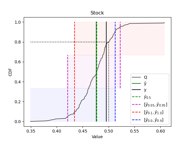
Figure 1 illustrates how the CPD can form one-sided and two-sided confidence intervals. It also illustrates how the probability of the true target falling below a given threshold can be determined. Or, conversely, it illustrates what threshold a specific probability does correspond to.
Compared to a CR, also able to provide valid confidence intervals from the underlying model, a CPS offers richer opportunities to define intervals and probabilities through querying of the CPD.
There are several different ways that difficulty () can be estimated, such as:
-
•
The (Euclidean) distances to the k nearest neighbors.
-
•
The standard deviation of the targets of the k nearest neighbors.
-
•
The absolute errors of the k nearest neighbors.
-
•
The variance of the predictions of the constituent models, in case the underlying model is an ensemble.
3.3 Factual and Counterfactual Explanations for Regression (CER and CCER)
In order to get CER, the probability intervals and a calibrated probability estimate from VA are exchanged for a confidence interval and the median which are derived from the CPD. The confidence interval is defined by user-selected lower and upper percentiles and allows dynamic selection of arbitrary confidence intervals.
Thus, for the algorithm to produce factual and counterfactual rules in the same way as for classification, the only thing that needs to be adjusted in the algorithm described in section 2.4.2 is to exchange the calibrator from VA to CPS. Since the confidence interval from CPS is based on the user-provided percentiles, the lower and upper percentiles are two necessary additional parameters. By default, the lower and upper percentiles are , resulting in a two-sided confidence interval derived from the CPD. One-sided intervals can in practice be handled as a two-sided interval with either or assigned as lower or upper percentiles. The calibrated probability estimate used in classification is exchanged for the median from the CPD, which in practice represents a calibration of the underlying model’s prediction, neutralizing any systematic bias in the underlying model. Consequently, using a CPS effectively enables CER with uncertainty quantification of both the prediction from the underlying model and each feature rule.
More formally, the confidence interval and the median is derived as follows:
-
1.
Use the calibration set to calculate the calibration residuals
-
2.
Fit a
ConformalPredictiveSystemmodel using the residuals. -
3.
Obtain the median and interval values
using the , the lower and the higher percentiles.
-
4.
To create CER following the procedure described in section 2.4.2 above, substitute and from the VA calibrator with and from the CPS.
- 5.
It is important to realize that since the input to the CER differ from CEC, not being probability estimates but instead actual predicted values, the CER will result in feature weights indicating changes in prediction rather than changes in probabilities.
If a difficulty estimator is used to get explanations based on normalized CPDs, is calculated using DifficultyEstimator in crepes.extras and passed along to both when fitting and obtaining median and interval values.
A minor difference between classification and regression is related to the discretizers that can be used. As both the BinaryEntropyDiscretizer and the EntropyDiscretizer require categorical target values for the calibration set, the BinaryDiscretizer and the DecileDiscretizer are recommended instead. These are automatically assigned based on the kind of problem and explanation that is extracted.
3.4 Factual and Counterfactual Probabilistic Calibrated Explanations for Regression (PCER and CPCER)
The simplest approach when trying to predict the probability that a target value is below (or above) a threshold is to treat the problem as a binary classification problem, with the target defined as
| (10) |
where are the regression targets, the threshold, and the binary classification target. To obtain the probability, some form of probabilistic classifier is used. If several different thresholds are of interest, or if each test instance needs a dynamic threshold based on some contextual information, this approach is infeasible.
The CPS makes it possible to query any regular regression model for the probability of the target falling below any given threshold. This effectively eliminates the need to treat the problem as a classification problem.
Utilizing this strength to create explanations is straightforward if it is only the probability that is of interest. However, achieving a calibrated explanation with uncertainty quantification for this scenario is not as straightforward as creating factual and counterfactual explanations for classification or regression. There is no obvious equivalent to the probability interval created by VA in classification or the confidence interval derived from a CPS in regression.
The fact that probabilistic predictions for regression can be achieved by viewing it as a classification problem holds a key to a solution. VA need a score for both the calibration and the test instances. By using a CPS as a probabilistic scoring function for both calibration and test instances, it becomes possible to use VA to calibrate the probability and provide a probability interval. The score used is the probability (from a CPD) of calibration and test instances being above the given threshold. The isotonic regressors used by VA also need a binary target for the calibration set, which is defined using equation (10).
Since the CPS is defined using the calibration set, the probabilities achieved on the same calibration set will be biased and consequently not be entirely trustworthy. To counteract that, the probability for each calibration instance is achieved by defining a CPS with all other calibration instances. More formally, the scores are derived as follows:
-
1.
Use the calibration set to calculate the calibration residuals where
-
2.
Fit a
ConformalPredictiveSystemmodel using the residuals . -
3.
Define the score for the test instance as .
-
4.
For each calibration instance :
-
a)
Use the residuals , i.e., the residuals for all calibration instances except instance , to fit a
ConformalPredictiveSystemmodel . -
b)
Calculate the score representing the probability of .
-
c)
Let represent the categorical target for calibration instance
-
a)
-
5.
Use as scores and as targets to define a VA calibrator, producing probability intervals and a calibrated probability estimate for and create a calibrated explanation using the description in section 2.4.2.
The solution presented above is preferable since it avoids bias when calculating the scores for the calibration set. However, it is also very computationally expensive. A much faster but somewhat biased solution would be to use the same to get the scores for both the calibration and test instances. This solution is used for normalized PCER and CPCER, to achieve reasonable computational performance.
The same discretizers as used for CER and CCER (see section 3.3) needs to be applied for PCER and CPCER, as it is motivated by the problem type. Furthermore, if normalized CPSs are to be used, is calculated using DifficultyEstimator in crepes.extras and passed along to and both when fitting and obtaining probability scores.
3.5 Summary of Calibrated Explanations
With the two solutions proposed here, Calibrated Explanations provide a number of possible use cases, which are summarized in Table 1. The general structure of factual and counterfactual explanations composed of lists of feature rules with conditions and feature weights or feature prediction estimates with confidence intervals (as described in Section 2.4) is general.
| Probabilistic | ||||
|---|---|---|---|---|
| Explanation | Characteristics | Classification | Regression | Regression |
| Regular Factual | Only prediction CI | TI | 5TI + 5LI + 5UI | 5TI |
| Uncertainty Factual | Rule + prediction CI | TI | 5TI | 5TI |
| Counterfactual | Only rule CI | TI | 5TI + 5LI + 5UI | 5TI |
3.6 Quality of Calibrated Explanations for Regression
The median from a CPD based on the calibration data can be seen as a form of calibration of the underlying model’s prediction, since it may adjust the prediction on the test instance to match what has previously been seen on the calibration set. The calibration will primarily affect systematic bias in the underlying model. Consequently, since CE calibrates the underlying model, it will create calibrated predictions and explanations. In addition, VA provides uncertainty quantification of both the probability estimates from the underlying model and the feature importance weights through the intervals for PCER. By using equality rules for categorical features and binary rules for numerical features (as recommended above), interpreting the meaning of a rule with a corresponding feature weight in relation to the target and instance value is straightforward and unambiguous and follows the same logic as for classification.
The explanations are reliable because the rules straightforwardly define the relationship between the calibrated outcome and the feature weight (for CER and PCER) or feature prediction estimate (for CCER and CPCER). The explanations are robust, i.e., consistent, as long as the feature rules cover any perturbations in feature values. Variation in predictions, e.g. when training using different training sets, can be expected to result in some variation in feature rules, corresponding to the variation in predictions. Obviously, the method does not guarantee robustness for perturbations violating a feature rule condition. The CER and CCER explanations are stable as long as the same calibration set and model are used. Finally, depending on the size of the calibration set which is used to define a CPS, the generation of CER is, in most cases, faster than or at least comparable to existing solutions such as LIME and SHAP. Generating a PCER will be slower than CEC since both require a VA to be trained. Compared to CEC, PCER will have some additional overhead from using a CPS on each calibration instance as well.
Finally, the calibrated predictions and their confidence intervals, which are an integral part of factual CE, provide the same guarantees as the calibration model used, i.e., the same guarantees as VA for classification and CPSs for regression (or a combination of both for probabilistic regression). However, even if the uncertainty quantification in the form of intervals for the feature rules are also derived from the same calibration model, these feature rule intervals do not necessarily provide the same guarantees. The reason is that the perturbed instances used in Step 2 in Section 2.4.2 are artificial and the combination of feature values may not always exist naturally in the problem domain. Whenever that happens, the underlying model and the calibration model will indicate that it is a strange instance but may not estimate the degree of strangeness correctly as there is no evidence in the data to base a correct estimate on.
4 Method
The implementation of both the regression and the probabilistic regression solutions is expanding the calibrated-explanations Python package [23] and relies on the ConformalPredictiveSystem from the crepes package [38]. By default, ConformalPredictiveSystem is used without normalization but DifficultyEstimator provided by crepes.extras is fully supported by calibrated-explanations, with normalization options corresponding to the list given at the end of Section 3.2.
4.1 Presentation of Calibrated Explanations trough Plots
In this paper, three different kinds of plots for CE are presented. The first two are used when visualizing CER. These plots are inspired by LIME, especially the rules in LIME have been seen as providing valuable information in the explanations.
-
•
Regular explanations, providing CE without any uncertainty information. These explanations are directly comparable to other feature importance explanation techniques like LIME.
-
•
Uncertainty explanations, providing CE including uncertainty intervals to highlight both the importance of a feature and the amount of uncertainty connected with its estimated importance.
For the reasons given in previous sections, CE is meant to use binary rules with factual explanations (even if all discretizers used by LIME can also be used by CE). One noteworthy aspect of CE is that the feature weights only show how each feature separately affects the outcome. It is possible to see pairwise combined weights through conjoined conjunctions of features (combining two or three different rules into a conjunctive feature rule). It is important to clarify that the feature weights do not convey the same meaning as in attribution-based explanations, like SHAP.
The third kind of plot is a counterfactual plot showing preliminary prediction estimates for each feature when alternative feature values are used.
Features rules are always ordered based on feature weight, starting with the most impactful rules. When plotting CE explanations, the user can choose to limit the number of rules to show. Factual explanations have one rule per feature. Counterfactual explanations, where CE creates as many counterfactual rules as possible, may result in a much larger number of rules, especially for categorical with many categories.
Internally, CE uses the same representation for both classification and regression. However, the plots visualizing the explanations have been adapted to suit the CER and PCER.
4.1.1 Calibrated Explanations Plots
The same kind of plots exists for regression as for classification. Compared to the plots used for classification, the regression plots differ in two essential aspects.
A common difference for both CER and CCER is that the feature weights represent changes in actual target values. For CER, this means that a feature importance of means that the actual feature value contributes with to the prediction. For a CCER, showing the prediction estimates with uncertainty intervals, the plot shows what the prediction is estimated to have been if the counterfactual condition would be fulfilled.
A difference that only applies to the factual plots is that the top of the plot omits the probabilities for the different classes and instead shows the median and the confidence interval as the prediction.
4.1.2 Probabilistic Calibrated Explanations Plots
Since the PCER represents feature importances as probabilities, just like CEC. The only difference needed for the plots for PCER compared to classification is to change the probabilities for a class label into probabilities for being below () or above () the given threshold.
4.2 Experimental Setup
The evaluation is divided into an introduction to CER, CCER, PCER, and CPCER through plots and an evaluation of performance. All plots are from the California Housing data set [39]. The underlying model in all experiments is a RandomForestRegressor from the sklearn package.
Our proposed algorithm is claimed to be fast, reliable, stable, and robust. These claims requires validation in an evaluation of performance. The explanations are reliable due to the validity of the uncertainty estimates used, i.e., the results achieved by querying the CPD, and from the uncertainty quantification of the feature weights or feature prediction estimates. Speed, stability and robustness will be evaluated in an experiment using the California Housing data set on a fixed set of test instances. Each experiment is repeated times using instances as a calibration set and test instances. The target values were normalized, i.e., . The following setups are evaluated:
-
•
CER: Factual explanation without normalization.
-
•
CER Var.: Factual explanation, with normalization based on the variance of the predictions of the constituent models in the underlying random forest regressor.
-
•
CCER: Counterfactual explanation without normalization.
-
•
PCER: Probabilistic factual explanation without normalization. The threshold is for all instances, i.e., the mid-point of the interval of possible target values.
-
•
LIME: LIME explanation.
-
•
LIME CPS: LIME explanation using the median from a CPD as prediction. The CPS was based on the underlying random forest regressor.
-
•
Tree SHAP: SHAP explanation. The
TreeExplainerclass is used, which is implemented in C++ and optimized for tree-based models, such as the underlying random forest regressor. -
•
SHAP CPS: SHAP explanation using the median from a CPD as prediction. The CPS was based on the underlying random forest regressor. Here, the
Explainerclass was used.
The evaluated metrics are:
-
•
Stability means that multiple runs on the same instance and model should produce consistent results. Stability is evaluated by generating explanations for the same predicted instances a 100 times with different random seeds. The largest variance in feature weight (or feature prediction estimate) can be expected among the most important features (by definition having higher absolute weights). The top feature for each test instance is identified as the feature being most important most often in the 100 runs (i.e., the mode of the feature ranks defined by the absolute feature weight). The variance for the top feature is measured over the 100 runs and the mean variance among the test instances is reported.
-
•
Robustness means that small variations in the input should not result in large variations in the explanations. Robustness is measured in a similar way as stability, but with the training and calibration set being randomly drawn and a new model being fitted for each run, creating a natural variation in the predictions of the same instances without having to construct artificial instances. Again, the variance of the top feature is used to measure robustness. The same setups as for stability are used except that each run use a new model and calibration set and that the random seed was set to in all experiments.
-
•
Computational speed is compared between the setups regarding explanation generation times (in seconds per instance). It was only the method call resulting in an explanation that was measured. Any overhead in initiating the explainer class has not been considered (it is assumed to be negligible). The closest equivalent to PCER would be to apply LIME and SHAP for classification to a thresholded classification model, as described in section 3.4. Since VA is comparably slow and PCER combines both CPSs and VA, with fitting and calls to a CPS for each calibration instance, it can be expected to be slow.
5 Results
The results are divided into two parts: 1) a presentation of CE through plots, explaining and showcasing a number of different available ways CE can be used and viewed; and 2) an evaluation of performance with comparisons to LIME and SHAP.
5.1 Presentation of Calibrated Explanations through Plots
In the following subsections, a number of introductory examples of CE are given for regression. First, factual and counterfactual explanations for regression are shown, followed by factual and counterfactual explanations for probabilistic regression.
5.1.1 Factual Calibrated Explanations for Regression
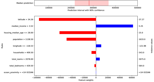
The regular CER plot in Fig. 2 illustrates the calibrated prediction of the underlying model as the solid red line at the top bar together with the confidence interval in light red. As can be seen, the house price is predicted to be $285K and with confidence, the price can be expected to be between [$215K-$370K]. Turning to the feature rules, the solid black line represents the median in the top-bar. The rule condition is shown to the left and the actual instance value is shown to the right of the lower plot area. The fact that this house is located more northbound (latitude > 34.26) has a large negative impact on the price (reducing it with $95K). On the other hand, since the median income is a bit higher (median income > 3.52), the price is pressed upwards with about $60K. Housing median age and population are two more features that clearly impact the price negatively.
When one-sided intervals are used instead, it is only the top-bar that is affected when using a regular CER plots. Figures 3(a) and 3(b) illustrate an upper bounded and a lower bounded explanation for the same instance, with the identical feature rule subplot omitted. As can be seen, the median (solid red line) is the same as before, while the confidence interval stretches one entire side of the bar. The upper bound ($330K in Fig. 3(a)) is lower and the lower bound ($240K in Fig. 3(b)) is higher compared to the two-sided CER plot in Fig. 2.


Fig. 4 illustrates an uncertainty plot for the same instance as before333Uncertainty plots are not available for one-sided explanations, as the visualization becomes obscured and hard to interpret. However, the one-sided uncertainty interval for each feature rule is calculated and can be accessed and used if needed.. When including uncertainty quantification in the CER plot, the feature importance has a light colored area corresponding to the span of possible contribution within the confidence used. The grey area surrounding the solid black line represents the same confidence interval as seen in the top bar. As can be seen, the northbound location still has a large negative impact but the span of uncertainty about exactly how large the impact covers about $150K, falling approximately within the interval [-$180K, -$30K]. The fact that part of the line is solid in color indicates that we can expect this feature to impact the price at least with -$30K, given the selected confidence level.
Looking at the other features, we can see that all of them include the median in the uncertainty interval, meaning that with 90% confidence, these features may impact the price in both directions. Obviously, both median income and in particular housing median age are more likely to have a positive and negative impact, respectively. Since no normalization have been used with this example, all the intervals are similar in width.
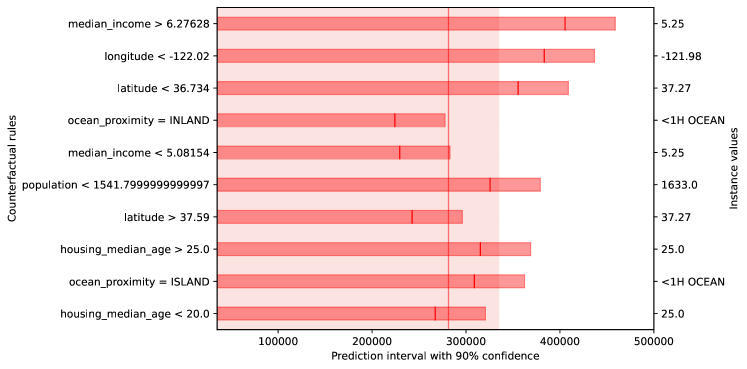
5.1.2 Counterfactual Calibrated Explanations for Regression
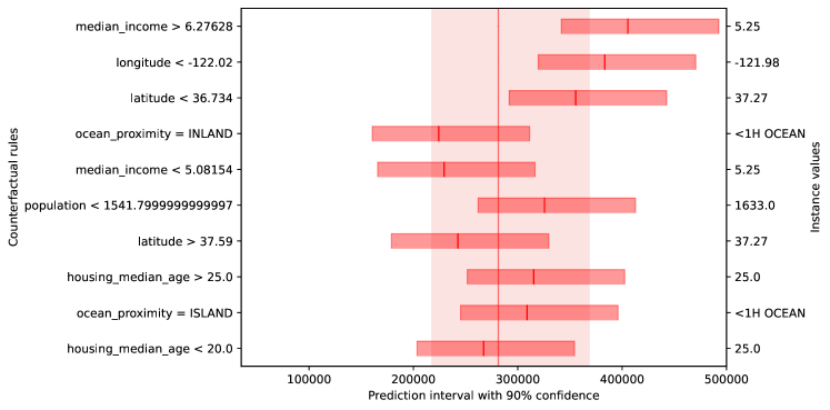
Turning to CCER, Fig. 5 shows a CCER plot for the same instance as before. Here, the solid line and the very light area behind it represent the median and the confidence interval of the calibrated prediction of the underlying model (i.e., the same as in Fig. 2). This is the ground truth that all the counterfactual feature rules should be contrasted against.
Contrary to CER, none of the rules cover the instance values in the CCER plot. Instead, there are several examples of the same feature being present in multiple rules. Here the interpretation is that the solid line and lighter red bar for each rule is the expected median and confidence interval achieved if the instance would have had values according to the rule. As an example, with everything else the same but median income > 6.28, then the expected price would be $405K with a confidence interval of [$340K, $490K]. It is also clear that if the house would have been located further south (latitude < 36.7), the price would go up, and if it would have been even further north (latitude > 37.6), the price would have gone down even further.
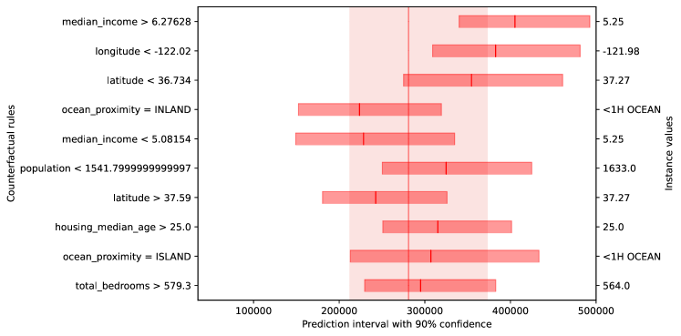
So far, all examples have used a standard CPS to construct the explanations (both CER and CCER), with the result that all confidence intervals are almost equal-sized. In Fig. 6, a difficulty estimator based on the standard deviation of the targets of the k nearest neighbors is used. The normalization will both affect the calibration of the underlying model, creating confidence intervals with varying sizes between instances, and the feature intervals. A crude assumption regarding the width of the feature intervals is that when the calibration set contains fewer instances covering an alternative feature value, the feature intervals will tend to be larger due to less information, and vice versa. This does not have to be the whole truth, as difficulty in this example is defined based on the standard deviation of the neighboring instances target values. As can be seen in Fig. 6, normalized CCER may generate rules resulting in both smaller and wider confidence intervals then the non-normalized rules.
Similarly to CER, CCER can also be one-sided. Fig. 7 shows an upper-bounded explanation with confidence. The interpretation of the first rule is that, with everything else as before, but median income > 6.28 the price will be below $450K with 90% certainty. Since the same CPS is used, the median is still the same as for a two-sided explanation.
5.1.3 Factual Probabilistic Calibrated Explanations for Regression
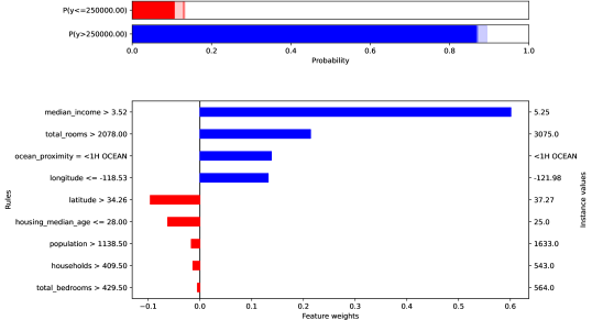
Fig. 8 shows a regular PCER plot for the same instance as above. In this plot, the possibility of querying the CPD about the probability of being below or above a given threshold is utilized. In this case, the threshold is set to a house price of $250K. Here, median income > 3.52 contributes strongly to the probability that the target is above $250K.
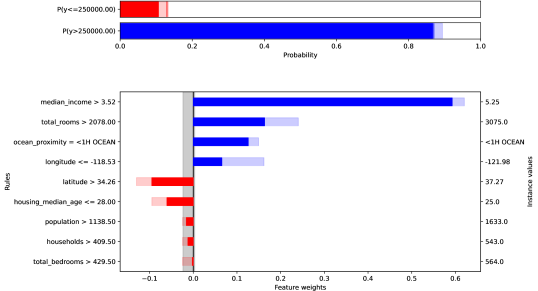
In Fig. 9, the same explanation is shown with uncertainties. As can be seen, the size of the uncertainty varies a lot between features, depending on the calibration of the VA calibrator.
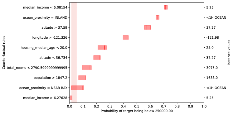
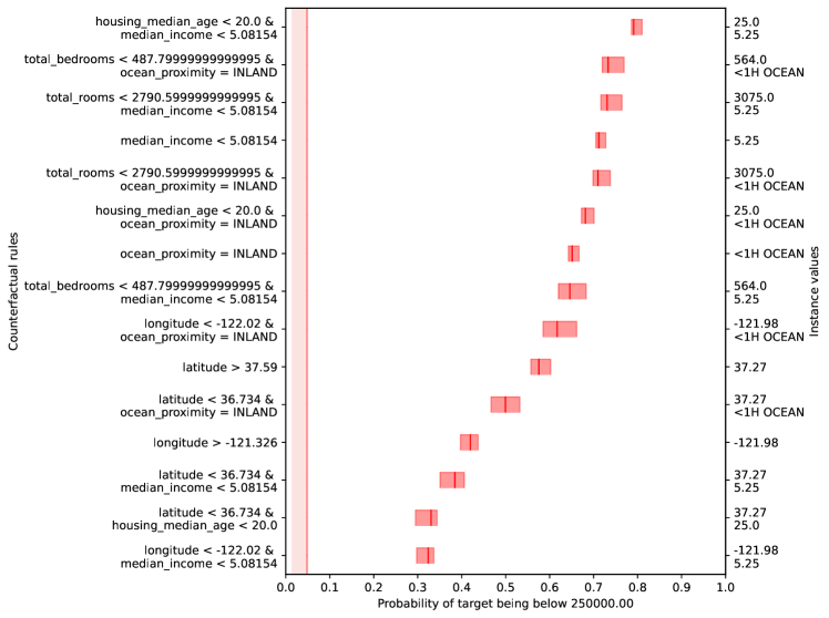
5.1.4 Counterfactual Probabilistic Calibrated Explanations for Regression
Fig. 10 shows a normalized CPCER plot for the same instance. In this case, the normalization used was based on the variance of the predictions of the trees in the random forest. The most influential rule relates to median income, with a lower income increasing the probability for a lower price. The normalization will affect the feature probability estimates and confidence intervals and may consequently also result in a different ordering of rules.
.
The final example, shown in Fig. 11, illustrates both conjunctive rules, combining two feature conditions in one rule, and normalization using the variance of the predictions of the trees in the random forest. Here, the number of rules to plot has been increased to 15. Here we see that conjunctive rules often result in more influential rules than single condition rules, illustrated by the majority of rules being conjunctive.
.
Factual or counterfactual rules can be generated without normalization or with any of the normalization options available in DifficultEstimator in crepes.extras. Conjunctive rules can be added at any time after the explanations are generated. All the examples shown here are from the same instance and the same underlying model, to showcase a subset of available ways the proposed solutions can be used. Further examples can be found in the code repository.
5.2 Performance Evaluation
Table 2 shows the results achieved regarding stability, robustness, and computational speed. Stability is measured using the mean variance when constructing explanations on the same instance using different random seeds, with lower values representing more stability. It is evident that both SHAP setups and all CE setups but PCER must be considered stable, since the mean variance is 0 (i.e., less than ). LIME and PCER, on the other hand, has a non-negligible mean variance, meaning that they are not, in comparison, as stable. The reason for why PCER is less stable is related to the sensibility of the probabilities derived from the CPD. The reason for the sensibility is that a relatively small change in prediction can easily result in a comparably much larger change in probability for exceeding the threshold, especially if the target is close to the threshold (which is set to , i.e., the mid-point in the interval of possible target values). Explanations using the median from a CPD and explanations using the underlying model result in similar stability levels.
Robustness is measured in a similar way as stability, but with a new model trained using different distributions of training and calibration instances between each run. The results achieved on robustness should be seen in relation to the variance in predictions from the underlying model on the same instances. The reason is that if the predictions that the explanations are based on fluctuate, then we can expect a somewhat similar degree of fluctuation in the feature weights as well, since they are defined using the predictions. The mean prediction variance is . Even if all the CE setups have higher mean variance compared to LIME and SHAP (i.e., are being less robust), it is still lower compared to the mean prediction variance. Furthermore, the explanations produced by the CE setups do not only rely on the crisp feature weight used to measure the mean variance but also include the uncertainty interval, highlighting the degree of uncertainty associated with each feature weight.
| CER | CER | CCER | PCER | LIME | LIME | Tree | SHAP | |
| Metric | Var. | CPS | SHAP | CPS | ||||
| Stability | 0 | 0 | 0 | 1.9e-5 | 3.9e-5 | 3.2e-5 | 0 | 0 |
| Robustness | 4.2e-4 | 3.7e-4 | 1.9e-3 | 3.9e-3 | 8.2e-5 | 8.6e-5 | 1.4e-4 | 1.4e-4 |
| Speed | 0.37 | 0.66 | 0.51 | 4.20 | 3.08 | 3.11 | 0.06 | 0.56 |
Regarding the computational speed, it should come as no surprise that Tree SHAP (TreeExplainer), implemented in C++, is fast when applied to a tree-based model like the random forest regressor. It is about times faster than when SHAP (Explainer) is applied on the median from CPD. In comparison, CER is slightly faster than SHAP CPS but clearly slower than Tree SHAP. CER is in turn about times faster than LIME which takes on average around seconds per instance. CER Var. (i.e., with normalization) should be expected to be slightly slower than CER, as the difficulty estimation requires some calculation. Also CCER, normally creating more rules than CER, is somewhat slower than CER. The slowest solution is PCER, having to calculate probabilities for all calibration instances as well as training two isotonic calibrators for each test instance. It is worth pointing out that PCER with normalization (not evaluated) becomes very much slower, as each calibration instance must apply a CPS. However, in the current implementation, the biased but faster solution discussed above are used for normalized PCER and CPCER.
6 Concluding Discussion
This paper extends Calibrated Explanations (CE), previously introduced for classification, with support for regression. Two primary use cases are identified: standard regression and probabilistic regression, i.e., measuring the probability of exceeding a threshold. The proposed solution relies on Conformal Predictive Systems (CPS), making it possible to meet the different requirements of the two identified use cases. The proposed solutions provide access to factual and counterfactual explanations with the possibility of conveying uncertainty quantification for the feature rules, just like CE for classification.
In the paper, the solutions have been demonstrated using several plots, showcasing some of the many ways that the proposed solutions can be used. Furthermore, the paper also includes a comparison with some of the best-known state-of-the-art explanation methods (LIME and SHAP). The results demonstrate that the proposed solution for standard regression is both stable and robust. Furthermore, it is reasonably fast, even if it cannot compete with the SHAP implementation in C++, optimized for tree models. The suggested solution is considered reliable for two reasons: 1) The calibration of the underlying model and 2) the uncertainty quantification, highlighting the degree of uncertainty of both prediction and feature weights.
The solution proposed to build probabilistic explanations for regression does not share all the benefits seen for standard regression. The solution has comparable performance as LIME, even if it is somewhat slower than LIME. The main strength of this solution is that it provides the possibility of getting probabilistic explanations in relation to an arbitrary threshold from any standard regression model without having to impose any restrictions on the regression model.
A Python implementation of the CE solution described in this paper is freely available with a BSD3-style license from:
-
•
Code repository: https://github.com/Moffran/calibrated_explanations
-
•
PyPi package: https://pypi.org/project/calibrated-explanations/
-
•
Documentation: https://calibrated-explanations.readthedocs.io/
Since it is on PyPI, it can be installed with pip install calibrated-explanations. The GitHub repository includes Python scripts to run the examples in this paper, making the results here easily replicable. The repository also includes several notebooks with additional examples. This paper details calibrated-explanations as of version 0.0.24.
6.1 Future Work
There are several directions for future work. Incorporating support for Mondrian CPSs, already supported by the crepes package, would be a natural first endeavor. One motivation for this is that Mondrian CPSs have been shown to remedy heteroscedasticity in the underlying model (e.g., often happening with ensemble models due to averaging affecting the boundery cases differently from the main mass of instances).
There are room for improvement regarding the plot layout and providing additional ways of visualization is a natural development in the future. This involves implementing support for explanations within image and text prediction, even if these improvements are more closely connected to classification problems.
An interesting area to look into is how this technique can be adapted to explanations of time-series problems. How to capture and convey the dependency between different time steps pose an interesting challenge.
Finally, the computational speed can probably be increased if implementing the core in C++ or by relying on fast languages being able to run Python code more efficiently, e.g., Mojo. The computational speed of probabilistic calibrated explanations can be dramatically improved by allowing the probability estimates of the calibration set to be biased. Further evaluation of the practical impact of such a change is warranted, to better understand the implications of making that trade-off.
Acknowledgments
The authors acknowledge the Swedish Knowledge Foundation and industrial partners for financially supporting the research and education environment on Knowledge Intensive Product Realization SPARK at Jönköping University, Sweden. Projects: AFAIR grant no. 20200223 and PREMACOP grant no. 20220187. Helena Löfström is a PhD student in the Industrial Graduate School in Digital Retailing (INSiDR) at the University of Borås, funded by the Swedish Knowledge Foundation, grant no. 20160035.
References
- \bibcommenthead
- Zhou et al. [2021] Zhou, J., Gandomi, A.H., Chen, F., Holzinger, A.: Evaluating the quality of machine learning explanations: A survey on methods and metrics. Electronics 10(5), 593 (2021)
- David Gunning [2017] David Gunning: Explainable Artificial Intelligence. Web. DARPA (2017). https://www.darpa.mil/attachments/XAIProgramUpdate.pdf Accessed 2019-08-29
- Ribeiro et al. [2016] Ribeiro, M.T., Singh, S., Guestrin, C.: ”Why Should I Trust You?”: Explaining the Predictions of Any Classifier. In: Proceedings of the 22nd ACM SIGKDD International Conference on Knowledge Discovery and Data Mining. KDD ’16, pp. 1135–1144. Association for Computing Machinery, New York, NY, USA (2016). https://doi.org/10.1145/2939672.2939778
- Alvarado-Valencia and Barrero [2014] Alvarado-Valencia, J.A., Barrero, L.H.: Reliance, trust and heuristics in judgmental forecasting. Computers in human behavior 36, 102–113 (2014)
- Buçinca et al. [2020] Buçinca, Z., Lin, P., Gajos, K.Z., Glassman, E.L.: Proxy tasks and subjective measures can be misleading in evaluating explainable ai systems. In: Proceedings of the 25th International Conference on Intelligent User Interfaces, pp. 454–464 (2020)
- Gunning and Aha [2019] Gunning, D., Aha, D.W.: Darpa’s explainable artificial intelligence program. AI Magazine 40(2), 44–58 (2019)
- Dimanov et al. [2020] Dimanov, B., Bhatt, U., Jamnik, M., Weller, A.: You shouldn’t trust me: Learning models which conceal unfairness from multiple explanation methods. Frontiers in Artificial Intelligence and Applications: ECAI 2020 (2020)
- Guidotti et al. [2018] Guidotti, R., Monreale, A., Ruggieri, S., Turini, F., Giannotti, F., Pedreschi, D.: A survey of methods for explaining black box models. ACM computing surveys (CSUR) 51(5), 1–42 (2018)
- Moradi and Samwald [2021] Moradi, M., Samwald, M.: Post-hoc explanation of black-box classifiers using confident itemsets. Expert Systems with Applications 165, 113941 (2021)
- Martens and Foster [2014] Martens, D., Foster, P.: Explaining data-driven document classifications. MIS Quaterly 38(1), 73–100 (2014)
- Slack et al. [2021] Slack, D., Hilgard, A., Singh, S., Lakkaraju, H.: Reliable post hoc explanations: Modeling uncertainty in explainability. Advances in neural information processing systems 34, 9391–9404 (2021)
- Rahnama and Boström [2019] Rahnama, A.H.A., Boström, H.: A study of data and label shift in the lime framework. arXiv preprint arXiv:1910.14421 (2019)
- Hoffman et al. [2018] Hoffman, R.R., Mueller, S.T., Klein, G., Litman, J.: Metrics for explainable ai: Challenges and prospects. Technical report, DARPA Explainable AI Program (2018)
- Carvalho et al. [2019] Carvalho, D.V., Pereira, E.M., Cardoso, J.S.: Machine learning interpretability: A survey on methods and metrics. Electronics 8(8), 832 (2019)
- Adadi and Berrada [2018] Adadi, A., Berrada, M.: Peeking inside the black-box: A survey on explainable artificial intelligence (xai). IEEE Access 6, 52138–52160 (2018)
- Wang et al. [2019] Wang, D., Yang, Q., Abdul, A., Lim, B.Y.: Designing theory-driven user-centric explainable ai. In: Proceedings of the 2019 CHI Conference on Human Factors in Computing Systems. CHI ’19, pp. 1–15. Association for Computing Machinery, New York, NY, USA (2019). https://doi.org/10.1145/3290605.3300831 . https://doi.org/10.1145/3290605.3300831
- Mueller et al. [2019] Mueller, S.T., Hoffman, R.R., Clancey, W., Emrey, A., Klein, G.: Explanation in human-ai systems: A literature meta-review, synopsis of key ideas and publications, and bibliography for explainable ai. Technical report, DARPA Explainable AI Program (2019)
- Agarwal et al. [2022] Agarwal, C., Krishna, S., Saxena, E., Pawelczyk, M., Johnson, N., Puri, I., Zitnik, M., Lakkaraju, H.: Openxai: Towards a transparent evaluation of model explanations. Advances in Neural Information Processing Systems 35, 15784–15799 (2022)
- Bhatt et al. [2021] Bhatt, U., Antorán, J., Zhang, Y., Liao, Q.V., Sattigeri, P., Fogliato, R., Melançon, G., Krishnan, R., Stanley, J., Tickoo, O., et al.: Uncertainty as a form of transparency: Measuring, communicating, and using uncertainty. In: Proceedings of the 2021 AAAI/ACM Conference on AI, Ethics, and Society, pp. 401–413 (2021)
- Vovk [2015] Vovk, V.: Cross-conformal predictors. Annals of Mathematics and Artificial Intelligence 74, 9–28 (2015)
- Platt et al. [1999] Platt, J., et al.: Probabilistic outputs for support vector machines and comparisons to regularized likelihood methods. Advances in large margin classifiers 10(3), 61–74 (1999)
- Vovk and Petej [2012] Vovk, V., Petej, I.: Venn-Abers predictors. arXiv preprint arXiv:1211.0025 (2012)
- Löfström et al. [2023] Löfström, H., Löfström, T., Johansson, U., Sönströd, C.: Calibrated Explanations: with Uncertainty Information and Counterfactuals (2023)
- Letzgus et al. [2022] Letzgus, S., Wagner, P., Lederer, J., Samek, W., Müller, K.-R., Montavon, G.: Toward explainable artificial intelligence for regression models: A methodological perspective. IEEE Signal Processing Magazine 39(4), 40–58 (2022)
- Vovk et al. [2005] Vovk, V., Gammerman, A., Shafer, G.: Algorithmic Learning in a Random World. Springer, Berlin, Heidelberg (2005)
- Vovk et al. [2019] Vovk, V., Shen, J., Manokhin, V., Xie, M.: Nonparametric predictive distributions based on conformal prediction. Mach. Learn. 108(3), 445–474 (2019)
- Molnar [2022] Molnar, C.: Interpretable Machine Learning, 2nd edn. Leanpub, ??? (2022). https://christophm.github.io/interpretable-ml-book
- Mothilal et al. [2020] Mothilal, R.K., Sharma, A., Tan, C.: Explaining machine learning classifiers through diverse counterfactual explanations. In: Proceedings of the 2020 Conference on Fairness, Accountability, and Transparency, pp. 607–617 (2020)
- Guidotti [2022] Guidotti, R.: Counterfactual explanations and how to find them: literature review and benchmarking. Data Mining and Knowledge Discovery, 1–55 (2022)
- Wachter et al. [2017] Wachter, S., Mittelstadt, B., Russell, C.: Counterfactual explanations without opening the black box: Automated decisions and the gdpr. Harv. JL & Tech. 31, 841 (2017)
- Löfström et al. [2022] Löfström, H., Hammar, K., Johansson, U.: A meta survey of quality evaluation criteria in explanation methods. In: De Weerdt, J., Polyvyanyy, A. (eds.) Intelligent Information Systems, pp. 55–63. Springer, Cham (2022)
- Alvarez-Melis and Jaakkola [2018] Alvarez-Melis, D., Jaakkola, T.S.: On the robustness of interpretability methods. arXiv preprint arXiv:1806.08049 (2018)
- Lundberg and Lee [2017] Lundberg, S.M., Lee, S.-I.: A unified approach to interpreting model predictions. In: Proceedings of the 31st International Conference on Neural Information Processing Systems, pp. 4768–4777 (2017)
- Ribeiro et al. [2016] Ribeiro, M.T., Singh, S., Guestrin, C.: ”why should i trust you?” explaining the predictions of any classifier. In: Proceedings of the 22nd ACM SIGKDD International Conference on Knowledge Discovery and Data Mining, pp. 1135–1144 (2016)
- Ribeiro et al. [2018] Ribeiro, M.T., Singh, S., Guestrin, C.: Anchors: High-precision model-agnostic explanations. In: Proceedings of the AAAI Conference on Artificial Intelligence, vol. 32 (2018)
- Vovk et al. [2004] Vovk, V., Shafer, G., Nouretdinov, I.: Self-calibrating probability forecasting. In: Advances in Neural Information Processing Systems, pp. 1133–1140 (2004)
- Lambrou et al. [2015] Lambrou, A., Nouretdinov, I., Papadopoulos, H.: Inductive venn prediction. Annals of Mathematics and Artificial Intelligence 74(1), 181–201 (2015)
- Boström [2022] Boström, H.: crepes: a python package for generating conformal regressors and predictive systems. In: Johansson, U., Boström, H., An Nguyen, K., Luo, Z., Carlsson, L. (eds.) Proceedings of the Eleventh Symposium on Conformal and Probabilistic Prediction and Applications. Proceedings of Machine Learning Research, vol. 179. PMLR, ??? (2022)
- Pace and Barry [1997] Pace, R.K., Barry, R.: Sparse spatial autoregressions. Statistics & Probability Letters 33(3), 291–297 (1997)