Medium Induced Mixing and Critical Modes in QCD

Abstract

The chiral crossover of QCD is expected to turn into a critical point at finite density. This is signaled by the emergence of an exactly massless critical mode which drives the critical behavior of the system. Based on phenomenological arguments, this mode is expected to be a mixture of chiral condensate and baryon number density fluctuations. We clarify the microscopic nature of this critical mode. Due to mixing induced at finite temperature and density, it turns out that this massless mode is composed of fluctuations in the chiral condensate, the neutral isoscalar omega vector-meson channel and the Polyakov loops. This is established using general arguments based on the analytic structure of the quark determinant at a critical point, and illustrated through explicit model calculations. Due to charge-conjugation symmetry breaking at finite density, the Hessian of the QCD effective action is non-Hermitian, but retains a symmetry under combined charge- and complex conjugation. This can give rise to a rich structure, potentially involving disorder lines, regimes with spatial modulations and instabilities in the phase diagram.

I Introduction

It is by now well established that QCD features a chiral crossover at small baryon chemical potential [1, 2, 3]. Model studies suggest that this crossover might turn into a critical endpoint (CEP) at larger chemical potential, where the transition is of second order [4, 5]. This expectation is supported by recent results of functional continuum methods, which have established that the chiral crossover becomes steeper as the chemical potential is increased [6, 7, 8, 9]. Assuming that no other phases emerge, these works indeed predict a CEP roughly around temperatures $T\approx 100$  MeV and baryon chemical potentials $\mu_{B}\approx 600$ MeV. While this does not exclude the possibility that other phases appear in this region which could wash-out the CEP, as discussed, e.g., in Refs. [10, 11], the overall indications of its existence by now are nevertheless rather strong.

The potential existence of a CEP has motivated experimental searches with ultrarelativistic heavy-ion collisions [12, 13, 14]. Many of these searches rely on the sensitivity of fluctuations in net-baryon multiplicities on the critical physics in the vicinity of the CEP [15, 16, 17, 18]. A non-monotonic beam-energy dependence has been proposed as a signature of a CEP in these works. Although it is now known that this is not a smoking-gun since this behavior can also arise from a steep crossover [19], there is little doubt that a system created in a heavy-ion collision is affected by critical physics if it evolves close enough to a CEP. Most notably, critical long-range correlations lead to equilibration times that exceed the timescales related to the expansion and cooling of matter in a heavy-ion collision [20, 21]. Due to this critical slowing down, the system will fall out of equilibrium. In addition to the symmetries and the dimensionality of the system which determine the static universal properties, additional conserved charges and hydrodynamic modes need to be taken into account [22] in order to describe the resulting dynamic universal behavior near the CEP [23].

At the CEP, the response of the system to certain static external perturbations, such as variations in the chemical potential, is singular. This is quantified by the divergence of the susceptibilities corresponding to these perturbations. In QCD, variations in the quark mass $m$ give rise to the chiral susceptibility $\chi_{m}$. It quantifies how the chiral condensate $\langle\bar{\psi}\psi\rangle$ changes as the quark mass changes. Since the chiral condensate is the order parameter of chiral symmetry breaking, $\chi_{m}$ diverges at the CEP. The chiral condensate is defined in the scalar quark-antiquark channel and it is therefore directly related to the vacuum expectation value of the scalar $\sigma$ meson. In typical low-energy effective model setups, as first shown in Ref. [24], a massless mode appears in the spacelike region of the $\sigma$ spectral function. This corresponds to the vanishing screening mass of the $\sigma$ which, in turn, is inversely proportional to the divergent correlation length at the CEP. This massless mode triggers singular behavior also in other susceptibilities, in particular the density and energy susceptibilities, which quantify the response of the baryon and energy densities to changes in the chemical potential and the temperature, respectively.

These insights have been used in Ref. [25] to argue that the actual critical mode should be a combination of the chiral condensate, the baryon number density and the entropy density. Including the dynamics of the coupled dissipative and diffusive fluctuations of chiral order parameter and conserved baryon density in an otherwise static medium, it has been shown that only one hydrodynamic mode is provided by the slow diffusive fluctuations of the latter [23], leading to the dynamic universality class of Model B [22]. If the motion of the medium is considered as well, coupling this mode to the energy-momentum tensor, from the potentially four additional hydrodynamic modes, only the two transverse components of the conserved momentum density lead to additional slow modes. Non-trivial reversible mode-mode couplings between these hydrodynamic modes then put the QCD CEP in the dynamic universality class of Model H [23], which is that of a liquid-gas transition in a pure fluid [22].

The central aspect of the preceding arguments, however, is the direct coupling between the chiral condensate and the baryon number density, which is usually taken into account in form of a phenomenological Ginzburg-Landau analysis. In this work we clarify the microscopic origin of this coupling. In particular, we show that at finite density a mixing between chiral condensate and baryon density, which can be identified with the temporal $\omega_{0}$ in the mesonic isoscalar vector channel, is induced on the level of the QCD path integral through the functional quark determinant. This is perhaps not surprising, but as it turns out, the underlying mechanism is more general, and in particular applies whenever a field or composite operator couples to the quarks in a way similar to the chemical potential. Interestingly, this is also the case for the Polyakov loop $\Phi$ and its conjugate $\bar{\Phi}$, which is used as an order parameter for confinement in the pure gauge theory and serves as a measure for nontrivial electric gluon correlations in finite temperature QCD as well. The existence of such a mixing has been noted previously [26], but its consequences have, to our knowledge, not been explored yet. Employing arguments based on the analytic structure of the free energy at the CEP, we use this to show that the true static critical mode is composed of $\langle\bar{\psi}\psi\rangle$, $\omega_{0}$, $\Phi$ and $\bar{\Phi}$. Possible implications on the critical dynamics are beyond the scope of our present work.

As already mentioned, scenarios alternative to a CEP at finite density cannot be excluded. In fact, most studies that find a CEP assume a homogeneous ground state. This includes state-of-the-art first-principles results from functional methods [6, 7, 8, 27]. An intriguing alternative is the emergence of inhomogeneous or crystalline phases with spatial modulations [5, 10]. Instead of a CEP, there could be a Lifshitz point in the phase diagram. A precursor for such phases, a moat regime where the particle energy is minimized at nonzero momentum [28, 29, 30], has recently been discovered in QCD in Ref. [7]. This is also relevant for heavy-ion collisions, where these regimes might leave observable signatures [29, 31, 32]. An efficient strategy to check if ground states other than a homogeneous one are favored is to test the stability of the system against small inhomogeneous fluctuations, see, e.g., Refs. [10, 33, 34, 35, 36, 37]. As pointed out in Refs. [38, 39] in the context of $\mathcal{PT}$-symmetric Euclidean field theories, mixing of fields can itself induce instabilities and spatially modulated structures. Consequently, in-medium mixing in QCD can quite naturally lead to these phenomena. We will explore this here in the vicinity of a CEP using low-energy models of QCD.

This paper is organized as follow. In Secs. II.1 and II.2 we derive the medium-induced mixing in QCD using a saddle-point expansion of the quark determinant. We then exploit the existence of a Yang-Lee edge singularity at the CEP to show that this mixing leads to a nontrivial modification of the critical mode, involving the chiral condensate, the isoscalar density and the Polyakov loops in Sec. II.3. In these sections, we also emphasize the relation of this mixing to the breaking of charge conjugation symmetry at finite density and discuss further possible physical implications. In Sec. III we illustrate our general arguments first with a Polyakov–Quark-Meson model in mean-field approximation in Sec. III.1, which effectively captures basic features of the QCD phase transition at low energies. After introducing the model and our approximations, we explicitly demonstrate that the soft mode at the CEP of this model is not carried by the $\sigma$ meson associated with the chiral condensate, but by a mixture of $\sigma$, $\Phi$ and $\bar{\Phi}$. In Sec. III.2 we add vector repulsion and vacuum fluctuations to this model. As anticipated, the critical mode then turns out to be a mixture of $\sigma$, $\omega_{0}$, $\Phi$ and $\bar{\Phi}$. Finally, before we conclude in Sec. V, we discuss the implications of in-medium mixing for the stability of the ground state in Sec. IV.

II Critical Mode

II.1 Induced mixing

We start by discussing how mixing through linear couplings to the chiral condensate arise in QCD at finite chemical potential. To this end, we note that fundamental interactions in QCD give rise to a Yukawa-type interaction between quarks and $\omega$ mesons, $\bar{\psi}\gamma^{\mu}\omega_{\mu}\psi$. This interaction arises from the resonance of a four-quark interaction in the isoscalar vector channel, $(\bar{\psi}\gamma^{\mu}\psi)^{2}$ and can be derived from first principles using, e.g., dynamical hadronization [40, 41, 7, 42]. For the present argument, we focus on the coupling between the quarks and $\omega_{0}$,

$$ih_{\omega}\bar{\psi}\gamma^{0}\omega_{0}\psi\,,$$ (1)

where $h_{\omega}$ is the relevant Yukawa coupling. Although this restriction is not necessary for the following arguments, we assume a repulsive vector interaction, so $ih_{\omega}$ has to be imaginary. This assumption is supported by nuclear matter phenomenology [43]. $\omega_{0}$ couples to the quark density in the same way as the quark chemical potential. Its equations of motion (EoM) can have nontrivial solutions in QCD, i.e. $\omega_{0}$ can acquire a vacuum expectation value (VEV). This VEV is necessarily related to the quark density $n_{q}$, so that

$$-i\bar{\omega}_{0}=\langle\omega_{0}\rangle\sim n_{q}\,.$$ (2)

We note that $\bar{\omega}_{0}$ is purely imaginary. Furthermore, we introduce a scalar field, $\sigma$, whose VEV is directly related to the chiral condensate,

$$\bar{\sigma}\sim\langle\bar{\psi}\psi\rangle\,.$$ (3)

It couples to the quarks through a Yukawa interaction,

$$h_{\sigma}\bar{\psi}\sigma\psi\,.$$ (4)

Chiral symmetry dictates that other fields, in particular pseudo-scalars, couple to the quarks in a similar way. But the details are irrelevant for the present discussion. The Dirac operator at finite chemical potential has the following form then:

$$\mathcal{M}=\gamma^{\mu}D_{\mu}+m+h_{\sigma}\sigma+\gamma^{0}(\mu+ih_{\omega}\omega_{0})\,,$$ (5)

where $m$ is the current quark mass and the covariant derivative in the fundamental representation is

$$D_{\mu}=\partial_{\mu}-igA_{\mu}\,,$$ (6)

with $A_{\mu}=A_{\mu}^{a}T_{a}$ with the $SU(N_{c})$ generators $T_{a}$, $a=1,\dots,N_{c}^{2}-1$. For now it is sufficient to work in Euclidean space. The logarithm of the functional determinant of $\mathcal{M}$ determines the contribution of quarks to the effective action, i.e. the generating functional of one-particle irreducible diagrams, of QCD. We are interested in finite temperature and density, where this determinant can be worked out by standard means of thermal field theory, see, e.g., Ref. [44]. It reads in the Matsubara formalism

$$\begin{split}\ln{\mathrm{det}}\mathcal{M}=T\sum_{n\in\mathbb{Z}}\int_{\mathbb{p}}\mathrm{tr}\ln M(\nu_{n},p)\,,\end{split}$$ (7)

with the operator

$$\begin{split}M(\nu_{n},p)&=i\gamma^{0}(\nu_{n}-gA_{0}+h_{\omega}\omega_{0}-i\mu)\\ &\quad+i\gamma^{j}(p_{j}-gA_{j})+m+h_{\sigma}\sigma\,.\end{split}$$ (8)

$\nu_{n}=\pi T(2n+1)$ are the fermionic Matsubara frequencies. The trace in this expression is over color-, flavor- and spinor-indices.

In a thermal medium the temporal gluon fields can have a nonzero VEV $\bar{A}_{0}=\langle A_{0}\rangle$ which is directly related to nontrivial VEV of the Polyakov loop [45]. Such a background field can always be rotated into the Cartan subalgebra of the gauge group and is thus assumed to be diagonal,

$$\bar{A}_{0}=\bar{A}_{0}^{(3)}T_{3}+\bar{A}_{0}^{(8)}T_{8}\,,$$ (9)

with $T_{a}=\frac{\lambda_{a}}{2}$ and the Gell-Mann matrices $\lambda_{a}$. In contrast, we can assume that the spatial gluon field has no VEV. On such a background, the quark propagator is given by

$$G_{\psi}(\nu_{n},\mathbb{p})=\frac{-i\gamma^{0}(\nu_{n}-g\bar{A}_{0}-i\bar{\mu})-i\gamma^{j}p_{j}+m_{q}}{(\nu_{n}-g\bar{A}_{0}-i\bar{\mu})^{2}+\mathbb{p}^{2}+m_{q}^{2}}\,,$$ (10)

where this is understood to be a diagonal matrix in color space with the diagonal elements of the gauge field background $\bar{A}_{0}$. We defined the constituent quark mass

$$m_{q}=m+h_{\sigma}\bar{\sigma}\,,$$ (11)

and the effective chemical potential

$$\begin{split}\bar{\mu}=\mu+ih_{\omega}\bar{\omega}_{0}\,.\end{split}$$ (12)

To see how mixing arises, it is instructive to consider a diagrammatic expansion first. To this end, we define the vertices

$$\Gamma_{\bar{\psi}\phi_{i}\psi}=\frac{\delta M}{\delta\phi_{i}(0)}\bigg{|}_{\rm EoM}\,.$$ (13)

Since we are interested in the soft modes relevant for criticality, we can restrict our analysis to zero momentum exchange. Hence, the functional derivatives are carried out at zero momentum and the delta distributions are omitted in favor of explicitly enforcing momentum conservation for all diagrams. The direct coupling between any two fields or operators $\phi_{i}$ and $\phi_{j}$ at zero momentum exchange generated from the quark determinant is then given by

$$\begin{split}\Gamma_{\phi_{i}\phi_{j}}&=\frac{\delta^{2}\ln{\mathrm{det}}\mathcal{M}}{\delta\phi_{i}(0)\delta\phi_{j}(0)}\bigg{|}_{\rm EoM}\\ &=T\sum_{n\in\mathbb{Z}}\int_{\mathbb{p}}\mathrm{tr}\,\Gamma_{\bar{\psi}\phi_{i}\psi}G_{\psi}(\nu_{n},\mathbb{p})\Gamma_{\bar{\psi}\phi_{j}\psi}G_{\psi}(\nu_{n},\mathbb{p})\,.\end{split}$$ (14)

From this expression we already see that certain linear couplings cannot be generated. This includes a mixing of the spatial gluons and the chiral condensate, $\Gamma_{\sigma A_{j}}=0$: With the vertices $\Gamma_{\bar{\psi}\sigma\psi}=h_{\sigma}$, $\Gamma_{\bar{\psi}A_{j}^{a}\psi}=-igT^{a}\gamma^{j}$ and the propagator in Eq. (10) it is evident that either the color or the spinor trace in Eq. (14) vanishes. The same reasoning leads to the absence of mixing between the $\omega_{0}$ and spatial gluon fields. Also the coupling between the chiral condensate and pions, $\Gamma_{\sigma\pi}$, vanishes since scalars cannot be transformed into pseudoscalars by quark exchange. Lastly, the mixing with spatial isoscalar vector mesons, $\Gamma_{\sigma\omega_{i}}$, can only occur at finite spatial momentum exchange.

In contrast, fields that couple to quarks similar to a chemical potential with a vertex $\sim\gamma_{0}$ can mix with the chiral condensate at vanishing spatial momentum. After the spinor trace, the integrand of Eq. (14) then is proportional to $(\nu_{n}-g\bar{A}_{0}-i\bar{\mu})$, which can lead to mixing in a medium.

Since the mixing we are considering here involves composite operators, a saddle point approximation is most convenient to extract the relevant linear couplings. It is sufficient to consider the contributions to the effective action from the quark determinant that arise from fluctuations $\delta\sigma$, $\delta\omega_{0}$ and $\delta A_{0}$ around the background fields $\bar{\sigma}$, $\bar{\omega}_{0}$ and $\bar{A}_{0}$. To leading order, the quark determinant then is

$$\begin{split}\frac{T}{\mathcal{V}}\ln{\mathrm{det}}\mathcal{\bar{M}}&=-2TN_{f}\int_{\mathbb{p}}\bigg{\{}\ln\Big{[}1+N_{c}\Phi e^{-(E_{\mathbb{p}}(\bar{\sigma})-\bar{\mu})/T}\\ &\quad+N_{c}\bar{\Phi}e^{-2(E_{\mathbb{p}}(\bar{\sigma})-\bar{\mu})/T}+e^{-3(E_{\mathbb{p}}(\bar{\sigma})-\bar{\mu})/T}\Big{]}\\ &\quad+\ln\Big{[}1+N_{c}\bar{\Phi}e^{-(E_{\mathbb{p}}(\bar{\sigma})+\bar{\mu})/T}\\ &\quad+N_{c}\Phi e^{-2(E_{\mathbb{p}}(\bar{\sigma})+\bar{\mu})/T}+e^{-3(E_{\mathbb{p}}(\bar{\sigma})+\bar{\mu})/T}\Big{]}\bigg{\}}\,,\end{split}$$ (15)

where $\mathcal{V}$ is the spatial volume. We neglected a vacuum contribution as it is irrelevant for our argument. Instead of the components of $\bar{A}_{0}$, it can be advantageous to use the temporal Wilson line,

$$P(\mathbb{x})=\mathcal{P}\exp\Bigg{[}ig\!\int_{0}^{\beta}\!dx_{0}\,A_{0}(x_{0},\mathbb{x})\Bigg{]}\,,$$ (16)

where $x_{0}$ is the Euclidean (imaginary) time coordinate and $\mathcal{P}$ denotes path ordering. The Polyakov loops are defined as

$$\begin{split}\Phi=\frac{1}{N_{c}}\langle\mathrm{tr}\,P\rangle\,,\quad\bar{\Phi}=\frac{1}{N_{c}}\langle\mathrm{tr}\,P^{\dagger}\rangle\,.\end{split}$$ (17)

For details see, e.g., Ref. [45]. The color trace on the $A_{0}$ background in the Cartan-subalgebra leads to the Polyakov loops in Eq. (15). Due to charge conjugation symmetry breaking, one has $\Phi\neq\bar{\Phi}$ at finite chemical potential.

By replacing $\bar{\phi}\rightarrow\bar{\phi}+\delta\phi$ with $\phi=(\sigma,\omega_{0},\Phi,\bar{\Phi})$, taking derivatives with respect to $\delta\phi$ and $\delta\tilde{\phi}$, where $\tilde{\phi}=(\sigma,\omega_{0},\bar{\Phi},\Phi)$, and then setting the fluctuating fields to zero, we can extract all the linear couplings between these operators at zero momentum exchange.

Treating the fluctuations requires some caution here. For the saddle point approximation to be well-defined, fluctuations must be in the direction of the steepest descent of the effective action. Put differently, the fluctuations $\delta\phi$ have to be along the stable Lefshetz thimble connected to $\bar{\phi}$ in field space, see, e.g., [46, 47]. The chiral condensate determines the constituent quark masses, so it is real. The scalar field fluctuations around it must be real as well. Similarly, a real free energy requires the Polyakov loops to be real for real chemical potentials. Note that the underlying eigenvalues of the gluon background field need to be complex in this case, see [48, 49, 50, 51] for related discussions. Regarding the vector meson, we have argued that the background field $\bar{\omega}_{0}$ needs to be pure imaginary in order for the density to be real. Since $\omega_{0}$ acts like a chemical potential, the effective action stays real for fluctuations $\delta\omega_{0}$ in either imaginary or real direction. Inspection of the quark determinant in Eq. (15) reveals that the dual (or unstable) thimble related to $\bar{\omega}_{0}$ is along the imaginary axis, while the stable thimble goes through $\bar{\omega}_{0}$ parallel to the real axis. Thus, we need to consider fluctuations of $\omega_{0}$ in real direction around an imaginary background.

Proceeding with the saddle point approximation, we find for the mixing between the chiral condensate and $\omega_{0}$,

$$\begin{split}\Gamma_{\sigma\omega_{0}}&=-4N_{f}T\sum_{n\in\mathbb{Z}}\int_{\mathbb{p}}\mathrm{tr}_{c}\frac{(\nu_{n}-g\bar{A}_{0}-i\bar{\mu})\,ih_{\omega}h_{\sigma}m_{q}}{\big{[}(\nu_{n}-g\bar{A}_{0}-i\bar{\mu})^{2}+\mathbb{p}^{2}+m_{q}^{2}\big{]}^{2}}\\ &=-4iN_{f}N_{c}h_{\omega}h_{\sigma}m_{q}\int_{\mathbb{p}}\frac{\partial}{\partial E_{\mathbb{p}}^{2}}\Big{[}N_{F}(E_{\mathbb{p}})-\bar{N}_{F}(E_{\mathbb{p}})\Big{]}\,,\end{split}$$ (18)

where $\mathrm{tr}_{c}$ denotes the color trace. We have furthermore introduced the modified distribution functions

$$\begin{split}N_{F}(E)&=\frac{1}{N_{c}}\mathrm{tr}_{c}n_{F}(E-\bar{\mu}+i\bar{A}_{0})\\ &=\frac{1+2\bar{\Phi}e^{(E-\bar{\mu})/T}+\Phi e^{2(E-\bar{\mu})/T}}{1+N_{c}\bar{\Phi}e^{(E-\bar{\mu})/T}+N_{c}\Phi e^{2(E-\bar{\mu})/T}+e^{3(E-\bar{\mu})/T}}\,,\\ \bar{N}_{F}(E)&=\frac{1}{N_{c}}\mathrm{tr}_{c}n_{F}(E+\bar{\mu}-i\bar{A}_{0})\\ &=\frac{1+2\Phi e^{(E+\bar{\mu})/T}+\bar{\Phi}e^{2(E+\bar{\mu})/T}}{1+N_{c}\Phi e^{(E+\bar{\mu})/T}+N_{c}\bar{\Phi}e^{2(E+\bar{\mu})/T}+e^{3(E+\bar{\mu})/T}}\,,\end{split}$$ (19)

where $n_{F}(x)=(e^{x/T}+1)^{-1}$ is the Fermi-Dirac distribution, and we have defined the quark energy $E_{\mathbb{p}}=\sqrt{\mathbb{p}^{2}+m_{q}^{2}}$. At $\bar{\mu}=0$, Polyakov loop and anti-loop are identical, $\Phi=\bar{\Phi}$, and $\Gamma_{\sigma\omega_{0}}$ vanishes for all temperatures. At $T=0$, this can already be inferred from the first line in Eq. (18) which then becomes an odd function of frequency for $\mu=0$. At finite density the degeneracy between $\Phi$ and $\bar{\Phi}$ is lifted and we conclude that $\Gamma_{\sigma\omega_{0}}\neq 0$, if $\mu\neq 0$. As a consequence of the repulsive nature of the vector interaction, this coupling is imaginary. We will comment on the physical consequences of this in the next section.

Next, we investigate the linear coupling between the Polyakov loops and the chiral condensate, $\Gamma_{\sigma\Phi}$ and $\Gamma_{\sigma\bar{\Phi}}$. This is related to fluctuations of $A_{0}$. Because the quark propagator in Eq. (10) is diagonal in color, only temporal gluons with nonzero diagonal elements can contribute. Without loss of generality, we can therefore assume that $A_{0}$ stays in the Cartan-subalgebra, and consider fluctuations in the Polyakov loops for simplicity instead. These lead to

$$\begin{split}\Gamma_{\sigma\Phi}&=2N_{f}N_{c}h_{\sigma}m_{q}\int_{\mathbb{p}}\frac{1}{E_{\mathbb{p}}}\bigg{\{}e^{2(E_{\mathbb{p}}-\bar{\mu})/T}\,K(\Phi,\bar{\Phi})\\ &\quad\times\Big{[}N_{F}(E_{\mathbb{p}})-N_{c}N_{F}(E_{\mathbb{p}})^{2}\Big{]}\\ &\quad+e^{(E_{\mathbb{p}}+\bar{\mu})/T}\,K\big{(}\bar{\Phi},\Phi\big{)}\,\Big{[}2\bar{N}_{F}(E_{\mathbb{p}})-N_{c}\bar{N}_{F}(E_{\mathbb{p}})^{2}\Big{]}\bigg{\}}\,,\end{split}$$ (20)

where we have defined

$$K(\Phi,\bar{\Phi})=\frac{1}{1+2\bar{\Phi}e^{(E_{\mathbb{p}}-\bar{\mu})/T}+\Phi e^{2(E_{\mathbb{p}}-\bar{\mu})/T}}\,.$$ (21)

The corresponding coupling between the anti-loop and the chiral condensate is analogously given by

$$\begin{split}\Gamma_{\sigma\bar{\Phi}}&=2N_{f}N_{c}h_{\sigma}m_{q}\int_{\mathbb{p}}\frac{1}{E_{\mathbb{p}}}\bigg{\{}e^{2(E_{\mathbb{p}}-\bar{\mu})/T}\,K(\Phi,\bar{\Phi})\\ &\quad\times\Big{[}2N_{F}(E_{\mathbb{p}})-N_{c}N_{F}(E_{\mathbb{p}})^{2}\Big{]}\\ &\quad+e^{(E_{\mathbb{p}}+\bar{\mu})/T}\,K(\bar{\Phi},\Phi)\,\Big{[}\bar{N}_{F}(E_{\mathbb{p}})-N_{c}\bar{N}_{F}\big{(}E_{\mathbb{p}})^{2}\Big{]}\bigg{\}}\,.\end{split}$$ (22)

This shows that chiral condensate and temporal gluon fields mix at finite temperature. The argument is sufficiently general to apply to QCD. Note that the two mixing terms in (20) and (22) are different at finite $\mu$.

We also find a nontrivial mixing between $\omega_{0}$ and the Polyakov loops,

$$\begin{split}\Gamma_{\omega_{0}\Phi}&=-2iN_{f}N_{c}h_{\omega}\int_{\mathbb{p}}\bigg{\{}e^{(E_{\mathbb{p}}-\bar{\mu})/T}\,K(\Phi,\bar{\Phi})\\ &\quad\times\Big{[}N_{F}(E_{\mathbb{p}})-N_{c}N_{F}(E_{\mathbb{p}})^{2}\Big{]}\\ &\quad-e^{2(E_{\mathbb{p}}+\bar{\mu})/T}\,K(\bar{\Phi},\Phi)\,\Big{[}2\bar{N}_{F}(E_{\mathbb{p}})-N_{c}\bar{N}_{F}(E_{\mathbb{p}})^{2}\Big{]}\bigg{\}}\,,\end{split}$$ (23)

and

$$\begin{split}\Gamma_{\omega_{0}\bar{\Phi}}&=-2iN_{f}N_{c}h_{\omega}\int_{\mathbb{p}}\bigg{\{}e^{2(E_{\mathbb{p}}-\bar{\mu})/T}\,K(\Phi,\bar{\Phi})\\ &\quad\times\Big{[}2N_{F}(E_{\mathbb{p}})-N_{c}N_{F}(E_{\mathbb{p}})^{2}\Big{]}\\ &\quad-e^{(E_{\mathbb{p}}+\bar{\mu})/T}\,K(\bar{\Phi},\Phi)\,\Big{[}\bar{N}_{F}(E_{\mathbb{p}})-N_{c}\bar{N}_{F}\big{(}E_{\mathbb{p}})^{2}\Big{]}\bigg{\}}\,.\end{split}$$ (24)

Note that these two couplings are pure imaginary and unequal at finite $\mu$ as well.

Finally, there are "off-diagonal" couplings between the Polyakov loops themselves, as well,

$$\begin{split}\Gamma_{\Phi\Phi}&=2N_{f}N_{c}^{2}T\int_{\mathbb{p}}\bigg{\{}e^{4(E_{\mathbb{p}}-\bar{\mu})/T}\,K(\Phi,\bar{\Phi})^{2}\,N_{F}(E_{\mathbb{p}}\big{)}^{2}\\ &\quad+e^{2(E_{\mathbb{p}}+\bar{\mu})/T}\,K(\bar{\Phi},\Phi)^{2}\,\bar{N}_{F}(E_{\mathbb{p}})^{2}\bigg{\}}\,,\end{split}$$ (25)

and

$$\begin{split}\Gamma_{\bar{\Phi}\bar{\Phi}}&=2N_{f}N_{c}^{2}T\int_{\mathbb{p}}\bigg{\{}e^{2(E_{\mathbb{p}}-\bar{\mu})/T}\,K(\Phi,\bar{\Phi})^{2}\,N_{F}(E_{\mathbb{p}})^{2}\\ &\quad+e^{4(E_{\mathbb{p}}+\bar{\mu})/T}\,K(\bar{\Phi},\Phi)^{2}\,\bar{N}_{F}(E_{\mathbb{p}})^{2}\bigg{\}}\,.\end{split}$$ (26)

Again, these two couplings are identical at $\mu=0$, but this degeneracy is lifted at nonzero $\mu$. This exhausts all mixing terms considered here.

The diagonal elements of the two-point function, $\Gamma_{\sigma\sigma}$, $\Gamma_{\omega_{0}\omega_{0}}$ and $\Gamma_{\Phi\bar{\Phi}}$, are also nontrivial and we list them here for completeness:

$$\Gamma_{\sigma\sigma} =2N_{f}N_{c}h_{\sigma}^{2}\int_{\mathbb{p}}\Bigg{\{}\Bigg{(}\frac{1}{E_{\mathbb{p}}}-\frac{m_{q}^{2}}{E_{\mathbb{p}}^{3}}+\frac{m_{q}^{2}}{E_{\mathbb{p}}^{2}}\frac{\partial}{\partial E_{\mathbb{p}}}\Bigg{)}$$

$$\quad\times\Big{[}N_{F}(E_{\mathbb{p}})+\bar{N}_{F}(E_{\mathbb{p}})\Big{]}\Bigg{\}}\,,$$

$$\Gamma_{\omega_{0}\omega_{0}} =-2N_{f}N_{c}h_{\omega}^{2}\int_{\mathbb{p}}\frac{\partial}{\partial E_{\mathbb{p}}}\Big{[}N_{F}(E_{\mathbb{p}})+\bar{N}_{F}(E_{\mathbb{p}})\Big{]}\,,$$

$$\Gamma_{\Phi\bar{\Phi}} =2N_{f}N_{c}^{2}T\int_{\mathbb{p}}\bigg{\{}e^{3(E_{\mathbb{p}}-\bar{\mu})/T}\,K(\Phi,\bar{\Phi})^{2}\,N_{F}(E_{\mathbb{p}})^{2}$$

$$\quad+e^{3(E_{\mathbb{p}}+\bar{\mu})/T}\,K(\bar{\Phi},\Phi)^{2}\,\bar{N}_{F}(E_{\mathbb{p}})^{2}\bigg{\}}\,.$$ (27)

In summary, we have shown that QCD in a dense medium features a mixing of the chiral condensate, the quark density and the Polyakov loops. Hence, the physical degrees of freedom have to be mixtures of these (composite) fields. The physical relevance of this observation is discussed in the remainder of this work.

As discussed above, the VEV of $\omega_{0}$ is directly related to the density of the system, see Eq. (2). Thus, with $\Gamma_{\sigma\omega_{0}}$ in Eq. (18) we have provided a microscopic derivation of the mixing between the chiral condensate and the density. The relevance of this mixing for the physics of the QCD critical point has previously been discussed based on phenomenological arguments [25, 23]. Our analysis shows that this might not be the whole story, however, as further linear couplings to the chiral condensate emerge in QCD.

In-medium mixing in QCD is of course well known. For example the mixing between the vector and axial vector mesons due to interactions with pions in the heat bath [52], or the mixing between different Goldstone bosons at large baryon-, isospin- and strangeness chemical potentials [53]. In addition, our discussion is limited to the case of two degenerate quark flavors applied to critical physics. Following the same line of reasoning as above, it is straightforward to see that in general mixing in QCD is considerably more extensive. For example, taking into account the strange quark gives rise to additional mixing with the strange chiral condensate, or, in terms of mesons, a combination of $f_{0}(500)$ and $f_{0}(980)$. At finite spatial momentum, also the spatial components of $\omega_{\mu}$ contribute. If flavor symmetries are relaxed, e.g., through different chemical potentials, and also excited states are taken into account, the mixing proliferates further.

II.2 Induced Hessian

We have derived the medium induced mixing in terms of fundamental objects in QCD. But while the chiral condensate and the quark density can be identified with the vacuum expectation values of mesonic operators, the Polyakov loop itself cannot be interpreted as some sort of field. However, since it is the trace of an exponential of an $SU(N_{c})$ matrix, cf. Eqs. (16) and (17), we may express it in terms of the eigenvalues $\theta_{c}$ of this matrix,

$$\Phi=\frac{1}{N_{c}}\sum_{c=1}^{N_{c}}\Big{\langle}e^{ig\theta_{c}/T}\Big{\rangle}\,.$$ (28)

The eigenvalues obey $\sum_{c}\theta_{c}=0$, so there are $N_{c}-1$ independent eigenvalues. We use the following parametrization for QCD,

$$\theta_{1}=\frac{a_{3}}{2}+\frac{a_{8}}{2\sqrt{3}}\,,\quad\theta_{2}=-\frac{a_{3}}{2}+\frac{a_{8}}{2\sqrt{3}}\,,\quad\theta_{3}=-\frac{a_{8}}{\sqrt{3}}\,,$$ (29)

which leads to

$$\begin{split}\Phi&=\frac{1}{3}e^{\frac{ia_{8}}{2\sqrt{3}T}}\bigg{[}2\cos\bigg{(}\frac{a_{3}}{2T}\bigg{)}+e^{-\frac{3ia_{8}}{2\sqrt{3}T}}\bigg{]}\,,\\ \bar{\Phi}&=\frac{1}{3}e^{\frac{-ia_{8}}{2\sqrt{3}T}}\bigg{[}2\cos\bigg{(}\frac{a_{3}}{2T}\bigg{)}+e^{\frac{3ia_{8}}{2\sqrt{3}T}}\bigg{]}\,.\end{split}$$ (30)

This parametrization can be motivated by using that the Polyakov loop is related to a nonvanishing temporal gluon background field $\bar{A}_{0}$. This field can be rotated into the Cartan subalgebra, see Eq. (9), and we can identify the components of $\bar{A}_{0}$ with our parameters, $g\bar{A}_{0}^{(3)}=a_{3}$ and $g\bar{A}_{0}^{(8)}=a_{8}$. Hence, $a_{3}$ and $a_{8}$ can loosely be interpeted as eigenvalues of a temporal gluon background field. As has been noted previously, real Polyakov loops require a purely imaginary $a_{8}$ at finite density [48, 49, 50, 51]. We emphasize that the Polyakov loop is not the same as the exponential of $\bar{A}_{0}$, although both are linked to the confinig properties of QCD and can serve as order parameters for confinement in the pure gauge theory [54].

Most importantly, the parametrization Eq. (30) provides a natural way to express the Polyakov loops in terms of field-like variables $a_{3}$ and $a_{8}$. We can use this to define the Hessian, or mass matrix, of the QCD effective action,

$$H=\big{(}\Gamma_{\phi_{i}\phi_{j}}\big{)}\,,$$ (31)

which is understood to be a $4\!\times\!4$ matrix with $\phi=(\sigma,\omega_{0},a_{3},a_{8})$. The entries involving $a_{3}$ and $a_{8}$ are directly related to the couplings involving $\Phi$ and $\bar{\Phi}$ via

$$\Gamma_{\phi_{i}a_{3/8}}=\bigg{(}\frac{\partial\Phi}{\partial a_{3/8}}\bigg{)}\,\Gamma_{\phi_{i}\Phi}+\bigg{(}\frac{\partial\bar{\Phi}}{\partial a_{3/8}}\bigg{)}\,\Gamma_{\phi_{i}\bar{\Phi}}\,.$$ (32)

With this, the Hessian in Eq. (31) is, to leading order in the saddle point approximation, determined by the linear couplings derived in Sec. II.1. It follows from the analysis of the previous section that $H$ has nonzero off-diagonal elements in a medium. This implies that diagonalization is required and the physical degrees of freedom are linear combinations of these fields.

The nontrivial mixing found here is directly related to the breaking of charge conjugation symmetry, $\mathcal{C}$, at finite density. Since $\omega_{0}$ is a component of a vector field, under charge conjugation it transforms as $\mathcal{C}\omega_{0}=-\omega_{0}$. Because gauge fields transform as $\mathcal{C}A_{\mu}=-A_{\mu}^{t}$, under $\mathcal{C}$ the parameter $a_{8}$ changes sign and $\Phi$ and $\bar{\Phi}$ are exchanged. Nonzero $\Gamma_{\sigma\omega_{0}}$, $\Gamma_{\omega_{0}\Phi}$ and $\Gamma_{\omega_{0}\bar{\Phi}}$ therefore break $\mathcal{C}$-symmetry, reflecting the $\mathcal{C}$-symmetry breaking at finite density. $\mathcal{C}$ symmetry breaking also leads to $\Phi\neq\bar{\Phi}$. For the mixing terms this implies $\Gamma_{\sigma\Phi}\neq\Gamma_{\sigma\bar{\Phi}}$, $\Gamma_{\omega_{0}\Phi}\neq\Gamma_{\omega_{0}\bar{\Phi}}$ and $\Gamma_{\Phi\Phi}\neq\Gamma_{\bar{\Phi}\bar{\Phi}}$. This also implies that $a_{8}$ in Eq. (30) must be nonzero and imaginary at finite density, because the Polyakov loops are real. Hence, all off-diagonal terms of the Hessian in Eq. (31) involving either a repulsive $\omega_{0}$ or $a_{8}$ are purely imaginary at finite density and change sign under $\mathcal{C}$.

This shows that the Hessian becomes non-Hermitian if charge conjugation symmetry is broken. However, complex conjugation $\mathcal{K}$ exchanges $\Phi$ and $\bar{\Phi}$ by definition. The Polyakov loops therefore transform into themselves under $\mathcal{CK}$. Since all couplings with either a single $\omega_{0}$ or a single $a_{8}$ are imaginary, they change sign under $\mathcal{K}$. Putting all this together, we see that the system retains an antilinear $\mathcal{C}\mathcal{K}$ symmetry at finite density [55]. We will get back to this point at the end of the next section.

II.3 Criticality

If the order parameter is known, like the chiral condensate $\bar{\sigma}$ for the chiral phase transition, the second-order critical point can be identified, e.g., through the divergence of the slope of $\bar{\sigma}(T)$. While this is sufficient to locate the critical point, it says nothing about its nature. In order to identify the critical mode, we use that, following the work of Lee and Yang, a branch point of the thermodynamic potential $\bar{\Omega}(\mu)$, where we omit other arguments such as $T$ since they are irrelevant here, is expected to pinch the real chemical potential axis at the CEP [56, 57]. This branch point is called the Yang-Lee edge singularity (YLE). Away from the phase transition, e.g., at small $\mu$ in QCD, the YLE is the singularity in the complex $\mu$ plane closest to the real $\mu$ axis. In QCD, we identify the YLE as follows: We assume that the effective potential $\Omega(\phi)$ is continuously differentiable and the EoM,

$$\frac{\partial\Omega(\phi)}{\partial\phi_{i}}\bigg{|}_{\phi_{i}=\bar{\phi}_{i}}=0\,,$$ (33)

has solutions for all positive $T$ and complex $\mu$. The effective potential evaluated on the solution of the EoM defines the thermodynamic potential,

$$\bar{\Omega}(\mu)=\Omega\big{(}\bar{\phi}(\mu)\big{)}\,.$$ (34)

The implicit function theorem states that Eq. (33) can locally be inverted to give unique continuously differentiable functions $\bar{\phi}_{i}(\mu)$ as long as the Hessian

$$H(\mu)=\Bigg{(}\frac{\partial^{2}\Omega}{\partial\phi_{i}\partial\phi_{j}}\Bigg{)}\bigg{|}_{\rm EoM}$$ (35)

is invertible. Conversely, if $H(\mu)$ has at least one vanishing eigenvalue at $\mu_{\rm YLE}\in\mathbb{C}$, then $\bar{\phi}_{i}(\mu)$ is not differentiable at $\mu_{\rm YLE}$. In presence of a branch cut, this singularity corresponds to the branch point. Thus, the YLE is identified as the (complex) chemical potential, $\mu_{\rm YLE}$, where at least one of the eigenvalues of the Hessian becomes zero.

The mixing discussed in the previous section gives rise to a nontrivial Hessian which, for two degenerate quark flavors at vanishing momentum, is a $4\times 4$ matrix. Since we have shown that the off-diagonal entries are in general nonzero in the medium, it follows that neither the chiral condensate $\sigma\sim\langle\bar{\psi}\psi\rangle$ alone, nor a linear combination between only the condensate and the baryon density $\sim\omega_{0}$ can be the true critical mode of the CEP in QCD. It should rather be a mixture of the $\sigma$ field, the conserved isoscalar density $\omega_{0}$, and the Polyakov loops here representing the nontrivial electric gluon correlations at finite temperature in QCD.

Since the couplings $\Gamma_{\sigma\Phi}$ and $\Gamma_{\sigma\bar{\Phi}}$, or, equivalently, $\Gamma_{\sigma a_{3}}$ and $\Gamma_{\sigma a_{8}}$, are nonzero at $\mu=0$ as long as $T>0$, also the critical mode(s) of the chiral transition at small (or vanishing) quark mass has an admixture of the Polyakov loop. If the second order transition happens to be at zero current quark mass, it is likely of $O(4)$ universality and pions are additional critical modes. Since the pions cannot mix with the Polyakov loops, only the radial component of the static critical mode is affected by our argument.

The response of the system to changes in external parameters, such as $T$, $\mu$ or the current quark mass $m$, is characterized by the susceptibilities. They inherit the singular behavior at the CEP from the YLE. To see this, we note that if $\Omega(\phi)$ is the effective potential and we denote $X=(T,\mu,m)$, the EoM leads to

$$\frac{\partial\bar{\phi}_{i}}{\partial X_{a}}=-H_{ij}^{-1}\frac{\partial^{2}\Omega}{\partial\phi_{j}\partial X_{a}}\bigg{|}_{\rm EoM}\,.$$ (36)

Using this relation, we can derive for the static susceptibilities,

$$\chi_{ab}=\frac{d^{2}\bar{\Omega}}{dX_{a}dX_{b}}\,,$$ (37)

the identity

$$\chi_{ab}=\frac{\partial^{2}\bar{\Omega}}{\partial X_{a}\partial X_{b}}+\frac{\partial^{2}\Omega}{\partial X_{a}\partial\phi_{i}}H_{ij}^{-1}\frac{\partial^{2}\Omega}{\partial\phi_{j}\partial X_{b}}\bigg{|}_{\rm EoM}\,,$$ (38)

see also, e.g., Refs. [62, 51, 63]. The susceptibilities diverge at the CEP as a result of the YLE, because ${\mathrm{det}}\,H=0$ at the YLE and $H^{-1}\sim({\mathrm{det}}\,H)^{-1}$. Since the susceptibilities are only sensitive to ${\mathrm{det}}\,H$, not the individual eigenvalues, they in general cannot reveal the nature of the critical mode.

We close this section by further discussing the observation that the Hessian is not Hermitian if charge conjugation symmetry is broken, and its important consequences for the eigenvalues. As noted above, in this case an antilinear $\mathcal{C}\mathcal{K}$ symmetry remains. The Hessian and its complex conjugate then obey the relation

$$H=CH^{*}C\,,$$ (39)

where $C$ is a diagonal matrix with entries $-1$ for the components corresponding to the fields that lead to imaginary mixing and $+1$ everywhere else. In the notation of Eq. (31), we have

$$C={\rm diag}(1,-1,1,-1)\,.$$ (40)

This relation implies that $H$ and $H^{*}$ have the same set of eigenvalues. The eigenvalues of the Hessian are therefore either real or come in complex conjugate pairs. This can be induced by the competition between repulsive and attractive bosonic interactions or the lifted degeneracy between the Polyakov loop $\Phi$ and its conjugate $\bar{\Phi}$ at nonzero real baryon chemical potential [55, 49, 64, 65, 38]. The former can be deduced from the imaginary mixing $\Gamma_{\sigma\omega_{0}}\neq 0$ in Eq. (18), and the latter from $\Gamma_{\sigma\Phi}\neq\Gamma_{\sigma\bar{\Phi}}$ and $\Gamma_{\Phi\Phi}\neq\Gamma_{\bar{\Phi}\bar{\Phi}}$, cf. Eqs. (20), (22) and (25), (26). A combination of these effects emerge in the mixing $\Gamma_{\omega_{0}\Phi}\neq\Gamma_{\omega_{0}\bar{\Phi}}\neq 0$ in Eqs. (23) and (24). All this arises from the breaking of charge conjugation symmetry at $\mu>0$. If the eigenvalues happen to come in complex conjugate pairs, this indicates the existence of a disorder line in the phase diagram beyond which correlations feature spatial modulations [49, 38, 66].

III Model Studies

In order to understand the mixing in QCD and illustrate its consequences for the critical mode in more detail, it is instructive to do explicit calculations. To this end, we use well-established low-energy models based on the coupling between quarks, mesons and gluon background fields. We first employ a standard Polyakov–Quark-Meson (PQM) model as the simplest example of the main effect in Sec. III.1, and then consider a more complete model, which in addition features the repulsive vector interaction, in Sec. III.2.

PQM models are widely used as they describe various features of QCD at low energies, especially regarding thermodynamics and the phase structure, see [45] and references therein.

III.1 Polyakov–Quark-Meson model

Since the admixture of the Polyakov loops in the critical mode is perhaps the most surprising finding of this work, we first study a two-flavor PQM model which describes the low-energy dynamics of quarks, $\sigma$, pions and the Polyakov loops. The Euclidean action of this simple PQM model is

$$\begin{split}S_{\rm PQM}&=\int_{0}^{\beta}\!dx_{0}\int\!d^{3}x\,\Bigg{\{}\bar{\psi}\big{[}\gamma^{\mu}\partial_{\mu}+\gamma^{0}(\mu+iA_{0})\big{]}\psi\\ &\quad+\frac{h_{\sigma}}{2}\bar{\psi}\big{(}\sigma+i\gamma_{5}\boldsymbol{\pi}\cdot\boldsymbol{\tau}\big{)}\psi+\frac{1}{2}(\partial_{\mu}\sigma)^{2}+\frac{1}{2}(\partial_{\mu}\boldsymbol{\pi})^{2}\\ &\quad+V(\sigma,\boldsymbol{\pi})+U(\Phi,\bar{\Phi})\Bigg{\}}\,,\end{split}$$ (41)

where $x_{0}$ is imaginary time, $\beta=1/T$ and $\boldsymbol{\tau}$ are the Pauli matrices. Quarks and mesons are coupled with the Yukawa coupling $h$. The meson effective potential,

$$V(\sigma,\boldsymbol{\pi})=\frac{\lambda}{4}\big{(}\sigma^{2}+\boldsymbol{\pi}^{2}-\nu^{2}\big{)}^{2}-j\sigma\,,$$ (42)

consists of a chiral $O(4)$-symmetric part $\sim\lambda$ and a current $j$ that explicitly breaks this symmetry down to $O(3)$, reflecting the finite current quark mass and, consequently, a nonzero pion mass in the phase with spontaneously broken chiral symmetry, $j=f_{\pi}m_{\pi}^{2}$, with pion mass and decay constant $m_{\pi}$ and $f_{\pi}$. For the Polyakov-loop potential $U(\Phi,\bar{\Phi})$, we use a simple $Z(3)$ center-symmetric polynomial,

$$\frac{1}{T^{4}}U(\Phi,\bar{\Phi})=-\frac{b_{2}(T)}{2}\Phi\bar{\Phi}-\frac{b_{3}}{3}\big{(}\Phi^{3}+\bar{\Phi}^{3}\big{)}+\frac{b_{4}}{4}(\Phi\bar{\Phi})^{2}\,,$$ (43)

with the following Ansatz for the temperature dependent coefficient

$$b_{2}(T)=\sum_{n=0}^{3}a_{n}\,\bigg{(}\frac{T_{0}}{T}\bigg{)}^{n}\,.$$ (44)

This parametrization of the potential has been established in [67], where the parameters were fixed to reproduce the thermodynamics of the pure gauge theory. In particular, $T_{0}=270$ MeV is the corresponding critical temperature of the first-order deconfinement phase transition in $SU(3)$ pure Yang-Mills theory.

The free energy functional of the PQM model is

$$\begin{split}F&=\ln\int\!\mathcal{D}\phi\,\exp\Big{\{}-S_{\rm PQM}[\phi]\Big{\}}\\ &=\ln\int\!\mathcal{D}(A_{0},\sigma,\boldsymbol{\pi})\,\exp\Bigg{\{}-\int_{x}\bigg{[}\frac{1}{2}(\partial_{\mu}\sigma)^{2}+\frac{1}{2}(\partial_{\mu}\boldsymbol{\pi})^{2}\\ &\quad+V(\sigma,\boldsymbol{\pi})+U(\Phi,\bar{\Phi})\bigg{]}+\ln{\mathrm{det}}\,\mathcal{M}\big{(}A_{0},\sigma,\boldsymbol{\pi}\big{)}\Bigg{\}}\,,\end{split}$$ (45)

with $\phi=(\psi,\bar{\psi},A_{0},\sigma,\boldsymbol{\pi})$. We have integrated out the quarks in the second line, which gives rise to the functional determinant of the Dirac operator,

$$\begin{split}\mathcal{M}\big{(}A_{0},\sigma,\boldsymbol{\pi}\big{)}&=\gamma^{\mu}\partial_{\mu}+\gamma^{0}\big{(}\mu+iA_{0}\big{)}+\frac{h_{\sigma}}{2}\big{(}\sigma+i\gamma_{5}\boldsymbol{\pi}\cdot\boldsymbol{\tau}\big{)}\,.\end{split}$$ (46)

In mean-field approximation, assuming a homogeneous VEV $\bar{\phi}=(0,0,\bar{A}_{0},\bar{\sigma},0)$ and the gluon background is in the Cartan-subalgebra, the effective potential $\Omega=-TF/\mathcal{V}$ becomes

$$\begin{split}\Omega(\sigma,\Phi,\bar{\Phi})&=V(\sigma)+U(\Phi,\bar{\Phi})-\frac{T}{\mathcal{V}}\ln{\mathrm{det}}\,\mathcal{M}\big{(}A_{0},\sigma\big{)}\,.\end{split}$$ (47)

The functional determinant is identical to the one in Eq. (15) with the replacement $\bar{\mu}\rightarrow\mu$, since our model does not have vector mesons.

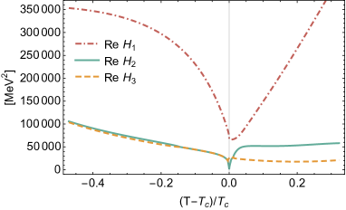
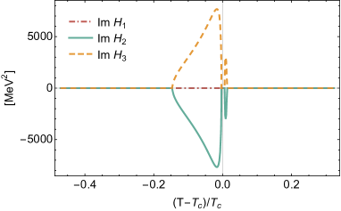
Figure 1: Eigenvalues $H_{1}$, $H_{2}$ and $H_{3}$ of the Hessian of the PQM model at the critical chemical potential as functions of $T$. The real and imaginary parts of these eigenvalues are shown in the left and right plot respectively.

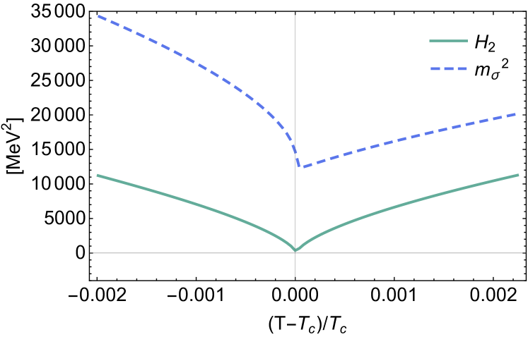
Figure 2: Scalar meson mass (dashed) and the eigenvalue $H_{2}$ of the Hessian (solid) as functions of $T$ close to the CEP. While the scalar meson mass stays finite at the CEP, the eigenvalue vanishes.

We fix the free parameters of the model as follows. The pion decay constant $f_{\pi}=93$ MeV is identified with $\bar{\sigma}$. We choose the explicit symmetry breaking such that in vacuum $m_{\pi}=138$ MeV. This fixes the value of the source $j$. The constituent quark mass in vacuum is set to $m_{q}=\frac{1}{2}h_{\sigma}f_{\pi}=300$ MeV, which fixes $h_{\sigma}$. The remaining model parameters are related to the physical quantities as follows: $\nu^{2}=f_{\pi}^{2}-m_{\pi}^{2}/\lambda$ and $\lambda=(m_{\sigma}^{2}-m_{\pi}^{2})/(2f_{\pi}^{2})$. We choose $m_{\sigma}=600$ MeV, so the remaining parameters are fixed. We emphasize that the latter two relations are strictly mean-field and only valid because we neglect the vacuum contribution of the quark determinant. Using dimensional regularization, this contribution renormalized the quartic meson coupling in vacuum with a term $\sim\phi^{4}\ln(\phi)$. However, since this term has no influence on the mixing, it is irrelevant for our qualitative discussion here. It will be taken into account for completeness in the next section.

The mixing between $\sigma$ and the Polyakov loops is identical to the one in Eqs. (20) and (22), as it is solely induced by the quark determinant in the PQM. The PQM has the Hessian

$$H_{\rm PQM}=\begin{pmatrix}\Omega_{\sigma\sigma}&\Omega_{\sigma a_{3}}&\Omega_{\sigma a_{8}}\\ \Omega_{\sigma a_{3}}&\Omega_{a_{3}a_{3}}&\Omega_{a_{3}a_{8}}\\ \Omega_{\sigma a_{8}}&\Omega_{a_{3}a_{8}}&\Omega_{a_{8}a_{8}}\end{pmatrix}\,,$$ (48)

with the entries $\Omega_{\phi_{i}\phi_{j}}=\frac{\partial^{2}\Omega}{\partial\phi_{i}\partial\phi_{j}}\big{|}_{\rm EoM}=\Gamma_{\phi_{i}\phi_{j}}$ given in Sec. II.1. The conversion from $\Phi$, $\bar{\Phi}$ to $a_{3}$, $a_{8}$ is done using Eqs. (30) and (32). Since $\Omega_{\sigma a_{8}}$ and $\Omega_{a_{3}a_{8}}$ are imaginary at $\mu\neq 0$, $H_{\rm PQM}$ is not Hermitian, but $\mathcal{C}\mathcal{K}$ symmetric. Thus, complex eigenvalues are allowed as long as they come in conjugate pairs. The existence of a disorder line is therefore possible in this model, cf. [49].

III.1.1 Screening masses and the critical mode

We now consider the static properties of the model. In order to identify the critical mode, it is important to clarify what the relevant mass is. For a general Euclidean propagator $G_{\chi}(p_{0},\mathbb{p})$ of a scalar field $\chi$, we can define two masses:

• pole mass: $G_{\chi}^{-1}(im_{\rm pole},\mathbb{0})=0$

• screening mass: $G_{\chi}^{-1}(0,im_{\rm scr}\,\mathbb{\hat{p}})=0$

The former is the mass of the particle that is relevant, e.g., for scattering processes. It represents the pole in the propagator of a stable particle at timelike momenta. The latter formally corresponds to a pole in the propagator at the spatial momentum variable $\mathbb{p}^{2}=-m_{\rm scr}^{2}$ and determines the large-distance behavior of the correlations in spatial directions. In fact [68], the screening mass

$$m_{\rm scr}={1}/{\xi}$$ (49)

is the inverse correlation length $\xi$ defined via

$$\lim_{|\mathbb{x}_{1}-\mathbb{x}_{2}|\rightarrow\infty}\big{\langle}\chi(t,\mathbb{x}_{1})\chi(t,\mathbb{x}_{2})\big{\rangle}\sim e^{-|\mathbb{x}_{1}-\mathbb{x}_{2}|/\xi}\,.$$ (50)

If $\chi$ is the critical mode, then its correlation length diverges at the CEP. Conversely, its screening mass vanishes. In this case, the order of the limits of temporal and spatial momenta going to zero is crucial. From the definition of the screening mass follows that at the CEP, if $\chi$ is the critical mode,

$$\lim_{|\mathbb{p}|\rightarrow 0}\,\lim_{p_{0}\rightarrow 0}G_{\chi}^{-1}(p_{0},\mathbb{p})=0\,.$$ (51)

Due to Landau damping in a thermal medium, these limits in general do not commute [69]. In order to extract the screening mass of the critical mode, the $p_{0}\rightarrow 0$ limit has to be taken first. This entails that we can extract the screening mass in Euclidean space, as it occurs for spacelike momenta. We can express the inverse propagator at $p_{0}=0$ as the sum of the tree-level contribution and self-energy corrections $\Pi(p_{0},\mathbb{p}^{2})$,

$$G_{\chi}^{-1}(0,\mathbb{p})=\mathbb{p}^{2}+m_{\chi}^{2}+\Pi(0,\mathbb{p}^{2})\,,$$ (52)

where we assumed symmetry of the system under spatial rotations. For the critical mode it is therefore sufficient to consider the renormalized mass

$$\bar{m}_{\chi}^{2}=m_{\chi}^{2}+\lim_{|\mathbb{p}|\rightarrow 0}\Pi(0,\mathbb{p}^{2})\,,$$ (53)

as it coincides with the screening mass at the CEP. This mass is also known as the curavture mass. This means that we can directly study the Hessian in Eq. (48). The mass of the critical mode, $\bar{m}_{\chi}$, is given by the eigenvalue of $H_{\rm PQM}$ which vanishes at the CEP.

To proceed, we solve the EoM for the effective potential in Eq. (47). By evaluating the second derivatives of the effective potential on the solutions $\bar{\phi}(T,\mu)$ we obtain he Hessian in Eq. (48). We identify the CEP through the YLE, i.e. through a vanishing eigenvalue of the Hessian at real chemical potential. With the parameters discussed above, we find

$$(T_{\rm CEP},\mu_{\rm CEP})\big{|}_{\rm PQM}\approx(189,164.5)\,{\rm MeV}\,,$$ (54)

where we emphasize that $\mu$ is the quark chemical potential.

In Fig. 1 we show the three eigenvalues $H_{1}$, $H_{2}$ and $H_{3}$ at $\mu=\mu_{\rm CEP}$ as a function of $T$. Their lengthy explicit expressions are not illuminating and hence not shown here. The first eigenvalue, $H_{1}$, coincides with the naive scalar meson (curvature) mass, $m_{\sigma}^{2}=\Omega_{\sigma\sigma}$, in vacuum. It is nonzero, also at the CEP. The eigenvalues $H_{2}$ and $H_{3}$ are associated with $\Omega_{a_{3}a_{3}}$ and $\Omega_{a_{4}a_{4}}$ in vacuum. We find extended regions around the CEP where the real parts of these eigenvalues, shown in the left plot of Fig. 1, are degenerate. In these regions they have imaginary parts with opposite signs but equal magnitude, see the right plot of Fig. 1. This is an explicit realization of the possibility of the $\mathcal{CK}$-symmetric Hessian to have complex conjugate pairs of eigenvalues, $H_{2}=H_{3}^{*}$. Thus, matter is in the complex regime of Ref. [38], where correlations exhibit spatial modulations. We return to this point in Sec. IV.

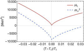
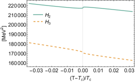
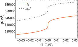
Figure 3: Eigenvalues $H_{1}$, $H_{2}$, $H_{3}$ and $H_{4}$ of the Hessian of the ${\rm PQM_{V}}$ at the critical chemical potential as functions of $T$. The first eigenvalue is compared to the naive $\sigma$ meson mass (dashed blue line in the left plot) and the fourth eigenvalue to the naive $\omega$ meson mass (dashed gray line in the right plot). Without mixing, i.e. in vacuum, $H_{1}$ corresponds to the squared $\sigma$ meson mass, $H_{4}$ to the squared $\omega$ mass and $H_{2}$ and $H_{3}$ to temporal gluon correlations at zero momentum.

Furthermore, $H_{2}$ shows a sharp drop at the CEP. In order to see the behavior near the CEP more clearly, we zoom in on $H_{2}$ in its vicinity in Fig. 2. We also show $m_{\sigma}^{2}$ in this region for comparison. Importantly, we observe that $m_{\sigma}^{2}$ does not vanish at the CEP. Thus, the naive scalar meson is not the critical mode. Its true nature is a mixture of the scalar meson and the Polyakov loops, or, loosely speaking, the eigenvalues of a temporal gluon background field. This is clearly demonstrated by the vanishing of $H_{2}$ at the CEP. We conclude that neither the curvature mass nor the screening mass of the sigma meson vanish at the CEP, but $\bar{m}_{\chi}^{2}=H_{2}$ does.

This confirms through an explicit example the general argument given in the previous section: In the presence of mixing, the YLE manifests itself in the eigenvalues of the resulting Hessian. As a consequence, the critical mode must be a mixture of the involved fields/operators, which are the scalar meson and the Polyakov loops in the PQM.

It is interesting to observe that the complex phase appears to be interrupted by the CEP. As seen in Fig. 1, $H_{2}$ is complex right before and after the CEP, but real in its immediate vicinity. This indicates that a CEP and the complex phase are mutually exclusive. While this is a conjecture at this point, it is physically sensible. In the complex phase, the correlation functions associated with the complex eigenvalues show exponentially damped oscillatory behavior at large distances [66]. The real part of the eigenvalue determines the inverse correlation length of these correlations, while the wave number of the oscillation is given by the imaginary part. At the CEP the correlation length diverges. If this were to happen in the complex phase, the correlation function would be an oscillatory function with infinite range. This is characteristic for an inhomogeneous phase and therefore contradicts the assumption of homogeneous solutions of the EoM that has been made to find the CEP in the first place.

We emphasize that the fact that only one eigenvalue vanishes implies that the CEP still belongs to the universality class of the $3d$ Ising model. So while the nature of the critical mode of the QCD critical point is different than expected, its static universality is unchanged. We expect that this conclusion does not change in the realistic case, where the $\omega_{0}$ is added to the mix as well. This is verified next.

III.2 Polyakov–Quark-Meson model with vector repulsion

As we have explicitly demonstrated in Sec. II.1 there is also a medium-induced mixing to the isoscalar density $\omega_{0}$ in the vector channel. We therefore add a repulsive vector interaction to the PQM of the previous section for completeness. This is achieved by adding the following corrections to the effective action shown in Eq. (41),

$$\begin{split}\Delta S&=\int_{0}^{\beta}\!dx_{0}\int\!d^{3}x\Bigg{\{}ih_{\omega}\bar{\psi}\gamma^{0}\omega_{0}\psi+\frac{1}{2}m_{\omega}^{2}\omega_{0}^{2}\Bigg{\}}\,,\end{split}$$ (55)

so that the effective action of the PQM with a repulsive vector interaction (${\rm PQM_{V}}$) is

$$S_{\rm PQM_{V}}=S_{\rm PQM}+\Delta S\,.$$ (56)

This is the minimal extension of the PQM to capture the mean-field effects of $\omega_{0}$. It can be derived from microscopic interactions by performing a Hubbard-Stratonovich transformation of an effective, point-like four-quark interaction in the repulsive temporal vector channel $\sim(\bar{\psi}\gamma^{0}\psi)^{2}$ . Of course, higher-order vector self-couplings and interactions between $\sigma$ and $\omega_{0}$ are also possible, but irrelevant for the present analysis. The thermodynamics of a similar model with an attractive $\omega_{0}$ interaction has been studied in [70].

Using that $\omega_{0}$ condenses at nonzero density, the resulting effective potential is

$$\begin{split}\Omega(\sigma,\omega_{0},\Phi,\bar{\Phi})&=V(\sigma)+\frac{1}{2}m_{\omega}^{2}\omega_{0}^{2}+U(\Phi,\bar{\Phi})\\ &\quad-\frac{T}{\mathcal{V}}\Big{[}\ln{\mathrm{det}}\,\mathcal{M}\big{(}A_{0},\sigma,\omega_{0}\big{)}\\ &\quad+\ln{\mathrm{det}}\,\mathcal{M}_{\rm vac}\big{(}\sigma\big{)}\Big{]}\,.\end{split}$$ (57)

The thermal part of the quark determinant is now identical to the one obtained from the leading order saddle point approximation in Eq. (15). In the spirit of a more complete model, we also take the renormalized vacuum contribution of the quark determinant into account. Following, e.g., [71, 72], and using that the $\omega_{0}$ mean-field acts like a chemical potential, it reads after dimensional regularization and minimal subtraction of the divergent piece,

$$\frac{T}{\mathcal{V}}\ln{\mathrm{det}}\,\mathcal{M}_{\rm vac}\big{(}\sigma\big{)}=N_{f}N_{c}\frac{h_{\sigma}^{4}\sigma^{4}}{2^{8}\pi^{2}}\ln\Bigg{(}\frac{h_{\sigma}^{2}\sigma^{2}}{4\Lambda^{2}}\Bigg{)}\,.$$ (58)

$\Lambda$ is the renormalization scale. This contribution renormalizes the quartic meson coupling $\lambda$ in Eq. (42) and as such affects the EoM of $\sigma$ and the scalar and pseudoscalar meson masses. This affects the parameters of the bosonic potential, for which we now choose $\nu=107$ MeV and $\lambda=20$. This yields $f_{\pi}=93.3$ MeV and $m_{\sigma}=477.7$ MeV. In addition, we fix the $\omega$ mass parameter as commonly done to $m_{\omega}=782$ MeV and set the vector Yukawa coupling to $h_{\omega}=1$. We note, however, that the only independent new parameter from the vector interaction is the ratio $m_{\omega}/h_{\omega}$, and that this parameter is not really related to the mass of the physical isoscalar vector meson. We refer to [73] for a related discussion. All other parameters are unchanged from above. We furthermore note that the vacuum fluctuations move the CEP to significantly smaller $T$ and larger $\mu$. We counteract this effect to some extent by choosing a smaller $m_{\sigma}$ as compared to the previous section. The resulting CEP is then at

$$(T_{\rm CEP},\mu_{\rm CEP})\big{|}_{\rm PQM_{V}}\approx(60.1,302)\,{\rm MeV}\,.$$ (59)

The Hessian is a $4\!\times\!4$ matrix,

$$H_{\rm PQM_{V}}=\begin{pmatrix}\Omega_{\sigma\sigma}&\Omega_{\sigma\omega_{0}}&\Omega_{\sigma a_{3}}&\Omega_{\sigma a_{8}}\\ \Omega_{\sigma\omega_{0}}&\Omega_{\omega_{0}\omega_{0}}&\Omega_{\omega_{0}a_{3}}&\Omega_{\omega_{0}a_{8}}\\ \Omega_{\sigma a_{3}}&\Omega_{\omega_{0}a_{3}}&\Omega_{a_{3}a_{3}}&\Omega_{a_{3}a_{8}}\\ \Omega_{\sigma a_{8}}&\Omega_{\omega_{0}a_{8}}&\Omega_{a_{3}a_{8}}&\Omega_{a_{8}a_{8}}\end{pmatrix}\,.$$ (60)

Contributions of the quark determinant to the entries of the Hessian are given by the expressions in Sec. II.1 plus a corresponding second derivative of the vacuum term in Eq. (58). The contributions from the purely bosonic part of the effective potential can be read off from Eqs. (42), (43) and (55). Again, the conversion from Polyakov loops to $\bar{A}_{0}$ eigenvalues is done by Eqs. (30) and (32).

We repeat the analysis of the eigenvalues of the Hessian near the CEP of this model as in the previous section. The results for the four eigenvalues of $H_{\rm PQM_{V}}$ at the critical chemical potential are shown in Fig. 3. In the small region around the CEP shown here, all eigenvalues are real and there is no complex regime. We note, however, that a complex regime arises, e.g., at larger temperature also in this model.

We compare the eigenvalues $H_{1}$ and $H_{4}$ in the left and right plot to the naive $\sigma$ and $\omega$ curvature masses, $m_{\sigma}^{2}=\Omega_{\sigma\sigma}$ and $m_{\omega}^{2}=\Omega_{\omega_{0}\omega_{0}}$. Again, due to the in-medium mixing the eigenvalues and these naive masses are not the same. Furthermore, analogous to the above, we find that the critical mode now is a mixture of $\sigma$, $\omega$ and the Polyakov loops. This is most clearly seen by the vanishing of $H_{1}$ at the CEP in the left plot of Fig. 3. Note that, as opposed to the result in the previous section, the critical mode is now in the direction which coincides with $\Omega_{\sigma\sigma}$ in the vacuum. For the present model it is also apparent that the naive curvature mass $\Omega_{\sigma\sigma}$ is in general unphysical, as it becomes negative close to the CEP. A similar observation has been made in models for nuclear matter with a repulsive vector interaction [65]. We emphasize that the CEP is signaled by the diverging susceptibility in Eq. (38). This is triggered by the vanishing of (at least) one eigenvalue of the Hessian. Some zero entry in the Hessian alone, e.g., $\Omega_{\sigma\sigma}=0$ as seen in the left plot of Fig. 3, is of no physical meaning in the presence of mixing.

IV Stability and Mixing

In order to determine the phase structure and thermodynamics of any system, the ground state has to be known. This is in general difficult to do and explicit solutions rely on assumptions about the structure of the ground state. For example, in the present case we have always assumed static, homogeneous ground states, i.e. $\bar{\sigma}$, $\bar{\omega}_{0}$, $\Phi$ and $\bar{\Phi}$ depend neither on time nor space. With very few exceptions in specific models, e.g., [74, 75], even the simplest gap equations that in principle allow for more complicated solution are impossible to solve exactly without relying on such assumptions. An efficient strategy to test whether the assumptions are correct is to perform a stability analysis. The general idea is to perturb the alleged ground state, e.g., by inhomogeneous fluctuations. If the perturbations decrease the free energy of the system, the assumptions that led to this ground state must be invalid and another ground state is favored. This strategy is, to some extent, agnostic to the true ground state, as it can only tell us that a given ground state is not the true ground state.

In case of models with only local interactions, an instability in mean-field approximation is equivalent to the static bosonic propagator having poles at real momenta, see, e.g., [10, 33, 34, 35, 36]. A generalization of this procedure based on the 2PI effective action, which is in principle not limited to mean-fields and able to handle non-localities that arise in realistic theories such as QCD, has recently been proposed in [37].

In any case, such a stability analysis in general relies on the knowledge of the momentum dependence of the self-energy corrections that arise from fluctuations. While this is sufficient to detect instabilities, it is not always necessary. To see this, recall from our discussion in Sec. III.1.1 that the Hessian corresponds to the static self-energy corrections at zero momentum. Hence, taking only these corrections into account, the inverse static propagator matrix is

$$G^{-1}(\mathbb{p})=\mathbb{p}^{2}+H\,,$$ (61)

where $H$ the $n\!\times\!n$ Hessian matrix. As already mentioned, the stability of the theory can be tested by studying the poles of the propagator in $\mathbb{p}^{2}$. They can be read off from the zeros of the equation

$${\mathrm{det}}(\mathbb{p}^{2}+H)=0\,.$$ (62)

This is a characteristic equation of $H$ with solutions $\mathbb{p}^{2}_{i}=-H_{i}$, where $i=1,\dots,n$ and $H_{i}$ are the eigenvalues of $H$. To be specific, these solutions tell us about the stability against small fluctuations around the bosonic ground state. The reason is that the one-loop corrections to the free energy from such fluctuations are given by $\sim\ln{\mathrm{det}}(\mathbb{p}^{2}+H)$. If the determinant becomes negative, the free energy becomes complex and the system is unstable [76]. We can therefore directly use the eigenvalues of the Hessian to perform a stability analysis. Since this does not take into account momentum-dependent self-energy corrections, such an analysis cannot detect all possible instabilities. However, owing to the nontrivial structure of the Hessian in the presence of mixing, certain instabilities can be detected with much less computational effort. This idea of doing a stability analysis based on mixing has been put forward in Ref. [38, 39] in the context of $\mathcal{PT}$-symmetric Euclidean scalar field theories.

In Euclidean space, ordinary screening poles are located at $\mathbb{p}_{i}^{2}\leq 0$. In this case the propagator decays exponentially and the correlation length is given by the screening masses, cf. Sec. III.1.1. These solutions correspond to real, positive eigenvalues $H_{i}$. If the solution contains complex conjugate pairs, as found in the PQM in Sec. III.1, the corresponding spatial correlator decays exponentially with a periodic oscillation indicative of a liquid-like behavior [66]. The correlation length in this case is determined by the real part of the eigenvalue, while the imaginary part fixes the wave number of the oscillation. This has been coined the complex regime in Ref. [38]. Both cases, real, positive $H_{i}$ and complex conjugate pairs, represent stable solutions. The free energy is real for any real spatial momentum.

Instabilities occur if at least one eigenvalue is negative. Then the static Euclidean propagator has a pole at $\mathbb{p}_{i}^{2}>0$ and the determinant in Eq. (62) is negative for some $\mathbb{p}^{2}\leq 0$. This typically entails that an inhomogeneous ground state with a wave number related to the pole position is favored. Following Ref. [39], these instabilities can be classified further: If there is an even number of negative eigenvalues, the propagator is positive at $\mathbb{p}^{2}=0$ but negative at nonzero momentum. Thus, the system is stable against homogeneous fluctuations, but has an inhomogeneous instability. For an odd number of negative eigenvalues, the propagator is already negative at $\mathbb{p}^{2}=0$ and the system is unstable against both homogeneous and inhomogeneous fluctuations. These two cases have been called patterned and unstable in Ref. [39], respectively.

We emphasize again that the underlying principle of this stability analysis is identical to the one of ordinary stability analyses. The difference is that medium-induced mixing itself can give rise to instabilities, even without nontrivial momentum-dependencies.

We can apply these ideas directly to the models investigated here. In the PQM model studied in Sec. III.1, we find either three positive or one positive and a pair of complex conjugate eigenvalues in the vicinity of the CEP. Hence, there are both an ordinary homogeneous and a complex phase around the CEP in the PQM at mean-field. In the ${\rm PQM_{V}}$ studied in Sec. III.2, we find four positive eigenvalues around the CEP and note that a complex phase arises at larger $T$ at the critical chemical potential. Hence, both models do not feature instabilities in the very narrow region of the phase diagram we considered here, but complex phases indeed arise. As discussed in Sec. III.1.1, a complex phase and a CEP could turn out to be mutually exclusive. However, further investigations are necessary to corroborate this.

V Conclusion

We have shown that the breaking of charge conjugation symmetry in a dense medium leads to an intricate mixing that directly affects the nature of the QCD critical point. This is established by exploiting that the CEP corresponds to a branch point, the Yang-Lee edge singularity, at real chemical potential. The medium-induced mixing between the chiral condensate, the $\omega_{0}$ and the Polyakov loops gives rise to a nontrivial Hessian. The branch point underlying the critical point leads to a vanishing eigenvalue of this matrix, while the naive screening masses remain nonzero in the presence of mixing. Thus, the critical mode is the eigenmode with vanishing eigenvalue at the CEP, involving a combination of the chiral condensate, the $\omega_{0}$ and Polyakov loops.

A side effect of $\mathcal{C}$ symmetry breaking is that the Hessian is not Hermitian anymore. This is induced in particular by a repulsive vector interaction and the lifted degeneracy between the expectation values of the Polyakov loop $\Phi$ and its conjugate $\bar{\Phi}$. Instead, there is a residual $\mathcal{C}\mathcal{K}$ symmetry and the Hessian can either have purely real eigenvalues or they come in complex conjugate pairs. This can give rise to a rich structure of the theory. In addition to an ordinary homogeneous phase, a disorder line can arise beyond which correlations feature spatial oscillations as in a liquid. The former is signaled by positive real eigenvalues of the Hessian, and the latter by complex conjugate pairs. Furthermore, even negative eigenvalues could occur which indicate the presence of an instability towards a different, possibly inhomogeneous phase.

We have studied the static eigenmodes near the CEP in different variations of the PQM model which exhibit these features in mean-field approximation. This allowed us to illustrate the physical consequences of medium-induced mixing using phenomenologically successful low-energy models of QCD. An exhaustive study of the parameter dependence and the full phase structure of these models in the presence of mixing is deferred to future work.

We emphasize that our analysis is not only valid for the CEP of QCD. It reveals the general structure of critical modes in the presence of mixing. For example, the same conclusions drawn here also apply to the liquid-gas transition of nuclear matter. While we focussed on the microscopic nature of the critical mode, in-medium mixing can also affect the universal properties of the system. Static universality is fully characterized by the susceptibilities which are, as we have argued, agnostic to the microscopic nature of the critical mode. This is different for dynamic universality. For example, the admixture of the $\omega_{0}$ to the critical mode modifies the dynamic universality class of the CEP since the $\omega_{0}$ condensate is in one-to-one correspondence with the conserved baryon density. This has been known on a phenomenological level for a long time, of course, and the present work only offers a more microscopic understanding in this regard. However, the strategy put forward here can readily be applied to other situations involving, e.g., different chemical potentials and conserved quantities.