Active Neural Mapping

Abstract

We address the problem of active mapping with a continually-learned neural scene representation, namely Active Neural Mapping. The key lies in actively finding the target space to be explored with efficient agent movement, thus minimizing the map uncertainty on-the-fly within a previously unseen environment. In this paper, we examine the weight space of the continually-learned neural field, and show empirically that the neural variability, the prediction robustness against random weight perturbation, can be directly utilized to measure the instant uncertainty of the neural map. Together with the continuous geometric information inherited in the neural map, the agent can be guided to find a traversable path to gradually gain knowledge of the environment. We present for the first time an active mapping system with a coordinate-based implicit neural representation for online scene reconstruction. Experiments in the visually-realistic Gibson and Matterport3D environment demonstrate the efficacy of the proposed method.

1 Introduction

How we represent a 3D environment accurately and efficiently is of tremendous importance for vision, robotics, and graphics communities. Recent advances in implicit neural representations (INRs) cast the issue as a low-dimensional function regression problem. Parameterized by a single network ${\bm{\theta}}$, the quantity of interest ${\bm{y}}$ such as color, occupancy, and semantics can be efficiently queried with the spatial coordinates ${\bm{x}}$ through a feedforward pass ${\bm{y}}=f({\bm{x}};{\bm{\theta}})$. Unlike traditional representations that discretize the entire space and explicitly store a set of the input-output samples $\{{\bm{x}}_{i},{\bm{y}}_{i}\}_{N}$ in manually-designed data structures such as voxel grid, surfel, and triangle mesh, the implicit neural representation is proved to have great capacity [71, 20, 81] that recovers complex signals at a constant small size, guaranteeing high-fidelity view synthesis [44, 4, 43] and accurate geometry reconstruction [67, 38, 3]. Nonetheless, the quality of the learned implicit neural representation is highly data-dependent: as implicit neural representations are trained through self-supervision given discrete training samples, insufficient sampling frequency leads to geometric and texturing artifacts [63, 80, 81, 62].

Figure 1: An overview of the proposed active neural mapping system. Guided by the continually-updated neural map (visualized as the SDF values through a forward pass), the mobile agent explores the environment actively to minimize the prediction uncertainty (visualized as the prediction error given the truth surface points).

Unlike conventional methods that rely on passive data acquisition, we address the problem of active neural mapping, where a 3D neural field is constructed on the fly with an actively-exploring mobile agent to best represent the scene. The target is to find efficient agent movement within the previously-unknown environment to gradually minimize the map uncertainty. Similar problems such as autonomous exploration and next-best-view planning are well-studied [13, 40, 77, 73, 52] by exploiting discretized scene representations to achieve the best coverage and reconstruction accuracy (see Sec. 2 for a detailed discussion). Though the implicit neural representation has its own merits, e.g. promising representation power and continuous/differentiable properties, this problem setting poses new challenges to the INRs: new knowledge of the environment is actively captured and constantly distilled to the neural map, where the neural map is expected to 1) specify the uncertain areas to be explored; 2) provide reliable geometric information for reconstruction; 3) allow for incremental updating given constantly observed data.

In this paper, we show for the first time a continual learning perspective of online active mapping based on the coordinate-based implicit neural representation. Inspired by the seminal works of [69, 78], we adopt the incremental updating of a continuous neural signed distance field. The key to our active mapping solution lies in a novel uncertainty quantification manner of the learned neural map through weight perturbation. We show empirically that the replayed buffer during continual learning forces the neural network to land in a low-loss basin given previously observed data to avoid forgetting, while resulting in a sharp ridge given erroneously-generated zero-crossings from not-well-explored areas to ensure transferability. That is to say, as the weight changes constantly during continual learning, the robustness of the predicted signed distance values exhibit distinguishable behaviors against weight perturbations for explored and unexplored surface samples. These findings share similar spirits with recent studies in neuroscience [39, 46, 21] and learning theory [76, 66], allowing us to explicitly reason the uncertain areas within the neural field and guide the mobile agent for actively capturing new information.

Our active mapping system adopts ideas from both frontier-based and sampling-based exploration strategies. The neural variabilities of zero-crossing samples are examined under random weight perturbations, where samples with high variation are viewed as target areas to be explored. Along with the continually-learned geometric information, the neural map guides the agent to explore the environment actively. The key contributions can be summarized as follows:

$\bullet$ We provide a new perspective of active mapping from the optimization dynamics of map parameters.

$\bullet$ We introduce an effective online active mapping system in a continual learning fashion.

$\bullet$ We propose a novel uncertainty quantification manner through weight perturbation for goal location identification.

2 Related Work

Active mapping.

Active mapping aims to find the optimal sensor movements to capture observations that best represent a scene, thus minimizing the uncertainty of the environment through exploration. Typical approaches can be categorized into frontier-based and sampling-based ones from a goal location identification perspective. Frontier-based methods explore by approaching the selected frontier (regions on the boundary between the explored free space and the unexplored space [77]), aiming to push the boundary of the explored areas until the entire space is observed. The major differences lie in the frontier detection strategies [85, 19, 65, 84, 6] and the best frontier selection strategies [14, 12, 27, 79].

On the other hand, sampling-based methods adopt random or guided sampling of potential viewpoints in the workspace and incrementally grow a Rapidly-exploring Random Tree (RRT) [35] or a Rapidly-exploring Random Graph (RRG) [30] to find the traversable paths. The next best view is repeatedly selected along the best branch in a receding horizon fashion [7] to maximize a given objective function. Unlike frontier-based methods that focus more on the map coverage, sampling-based methods allow different objectiveness, e.g., localization uncertainty [50], geometric uncertainty [59, 57, 24], visual saliency [15], and vehicle dynamics [18], to be taken into account.

To take advantage of both frontier-based and sampling-based methods, new strategies are employed in a hybrid or an informed sampling-based fashion. The hybrid method [60] adopts a sampling-based manner for local planning, while utilizing a frontier-based method for global planning to handle the dead-end case as sampling-based methods can easily get stuck locally. Meanwhile, as most computational resources are wasted on the redundant utility computation of non-selected samples [68, 5], the informed sampling based methods [32, 41, 56] are proposed that sample candidates around frontiers to ensure faster exploration.

Dense metric representations.

Dense metric representations play important roles in path planning as they provide complete geometric information for any queried location within the workspace. Existing active mapping methods mainly rely on the volumetric representation that discretizes the space into voxel grids. Occupancy grid map, for example, allows distinguishing between free, occupied, and unknown space. Most occupancy grid based methods are deployed in 2D [77, 10, 25] for tractable computation as a mobile device typically moves at a constant height [31]. There are also 3D extensions [7, 19, 6] that exploit an Octomap structure [28] for recursive updating of the occupancy status. Meanwhile, it is noted that merely occupancy information may be insufficient for certain gradient-based planners, CHOMP [87] for instance. Therefore, the Euclidean signed distance field (ESDF) is introduced to be updated incrementally from a truncated signed distance field (TSDF) [45, 49] or a 3D occupancy grid map [26] using Breadth-First Search (BFS), allowing online planning on a CPU-only platform.

Recent advances in implicit neural representations (INRs) [44, 51, 42, 11] facilitate multiple robotics-related downstream tasks. By encoding the coordinate-based scene properties in weights of a neural network, INRs are able to recover fine-grained scene properties with light-weight parameters [67, 71, 20, 81]. Hence, accurate scene geometry can be recovered with a single network [3, 38]. On the other hand, the gradient can be efficiently extracted from the continuous neural field through automatic differentiation. Together with the geometric information, a smooth trajectory can be optimized for collision avoidance [2, 33]. Recently, [36, 48]share a similar idea of refining a coarsely-trained NeRF by actively selecting new viewpoints for batch retraining. Inspired by the continual learning fashion of online neural field updating [78, 69, 86, 47], we extend the works to an online active mapping framework, where the implicit neural field is updated on the fly to guide the exploration for complete coverage and constant uncertainty reduction. There are also two concurrent works [55, 82] that are most related to ours, tackling the inward view selection and path planning for object reconstruction.

3 Preliminaries

Given an indoor environment as the workspace ${\mathcal{X}}\in{\mathbb{R}}^{3}$ that is unknown a prior, we aim to best represent the scene property of interest ${\mathcal{Y}}\in{\mathbb{R}}^{m}$ with a continuous function parameterized by a single MLP ${\bm{\theta}}$, establishing the mapping $f({\bm{x}};{\bm{\theta}}):{\mathcal{X}}\to{\mathcal{Y}}$ between spatial coordinates ${\bm{x}}\in{\mathcal{X}}$ and the corresponding scene property ${\bm{y}}\in{\mathcal{Y}}$. To obtain an optimal map representation, a mobile agent is deployed to actively capture sensory data $\{{\bm{x}}_{i},{\bm{y}}_{i}\}^{t}\sim{\bm{z}}^{t}\subset{\mathcal{D}}$ sampled from the scene surfaces ${\mathcal{D}}$ (depth sequence in our case) with self-decided control ${\bm{a}}^{t}$ at each time, and the map parameters ${\bm{\theta}}$ is updated incrementally with incoming observations.

From a global optimum view, the map can be optimized through empirical risk minimization given a pre-defined penalty function $\mathcal{L}$ and sufficient samples from the true distribution of ${\mathcal{D}}$ as:

$${\bm{\theta}}^{*}=\arg\min\mathbb{E}_{({\bm{x}},{\bm{y}})\sim{\mathcal{D}}}(\mathcal{L}({\bm{x}},{\bm{y}};{\bm{\theta}})).$$ (1)

In our case of an online setting, the continual learning of the map can be cast as minimizing a cumulative loss [54] within a time interval $[t,t+k]$ in the following steps as:

$${\bm{\theta}}^{t}=\arg\min\sum_{\tau=t}^{t+k}\lambda^{\tau}\mathbb{E}_{({\bm{x}}^{t},{\bm{y}}^{t})\sim{\bm{z}}^{1:\tau}}(\mathcal{L}({\bm{x}}^{t},{\bm{y}}^{t};{\bm{\theta}}^{t})),$$ (2)

where the observation ${\bm{z}}^{t}$ is conditioned on past controls ${\bm{a}}^{1:t}$, and $k\rightarrow\infty$ equals an unending exploration setting.

From Eq. 2, we can see that the overarching goal of an optimal map is intractable to be achieved as future observations ${\bm{z}}^{t:t+k}$ are not available. This issue is formalized by Raghavan and Balaprakash [54] from a generalization-forgetting perspective. They point out that the penalty ${\mathcal{L}}$ is needed to not only prevent catastrophic forgetting of previous observations, but improve generalization to new data. As proved in [54], the dynamics of continual learning are affected by three factors: the cost of prediction error over all past observations $\mathbb{E}_{({\bm{x}},{\bm{y}})\sim{\bm{z}}^{1:t}}(\mathcal{L}({\bm{x}},{\bm{y}};{\bm{\theta}}^{t}))$, the cost variation arising from the data distribution shift $\Delta{\bm{x}}^{t}$, and the cost variation arising from the parameter changes $\Delta{\bm{\theta}}^{t}$:

$$H(\delta{\bm{z}},{\bm{\theta}}^{t}) \approx\beta L({\bm{\theta}}^{t},{\bm{z}}^{1:t})$$ (3)

$$+\sum_{\tau=t}^{t+k}(L({\bm{\theta}}^{\tau},{\bm{z}}^{1:\tau}\cap\delta{\bm{z}})-L({\bm{\theta}}^{\tau},{\bm{z}}^{1:\tau}))$$

$$+\sum_{\tau=t}^{t+k}(L({\bm{\theta}}^{\tau}+\delta{\bm{\theta}},{\bm{z}}^{1:\tau})-L({\bm{\theta}}^{\tau},{\bm{z}}^{1:\tau})),$$

where $L({\bm{\theta}}^{i},{\bm{z}}^{j})=\mathbb{E}_{({\bm{x}}^{j},{\bm{y}}^{j})\sim{\bm{z}}^{j}}(\mathcal{L}({\bm{x}}^{j},{\bm{y}}^{j};{\bm{\theta}}^{i}))$.

Intuitively, minimal $H(\delta{\bm{z}},{\bm{\theta}}^{t})$ induced by distribution shift $\delta{\bm{z}}$ and parameter changes $\delta{\bm{\theta}}$ indicates that the arrival of a new observation does not affect the current optimal solution ${\bm{\theta}}^{t}$, thus achieving the global optimum. Even though such an optimum cannot be guaranteed, a saddle point can be found. In [54], the discrepancy between two subsequent tasks is maximized, followed by the minimization of forgetting under the maximum generalization. This manner lays the theoretic foundation for us to solve the active mapping problem: if we iteratively find the most distribution shift of $\delta{\bm{z}}$ and update the map parameters ${\bm{\theta}}$ given a new observation, we converge to a local equilibrium point within the small time interval $k$ according to Eq. 3.

The optimization perspective of Eqs. 2 and 3 well distinguishes the proposed problem setting, namely active neural mapping, from previous research. Recent INR-based passive SLAM systems [69, 86, 47] or multi-view stereopsis methods [44, 3, 83] merely minimize the first term in Eq. 3, while we further take the agent action optimization into account to serve as a local generalization maximizer. Consequently, the actively captured training samples can better mimic the actual distribution ${\mathcal{D}}$ compared to the passive observations ${\bm{z}}^{1:t}$. Compared to traditional active mapping methods, we explicitly conduct map optimization through back-propagation instead of the heuristically-designed fusion techniques. The goal location is decided in a data-driven manner (see Sec. 4 for details) instead of the ad-hoc goal location identification strategies. The objectiveness of active mapping in Eq. 3 allows for continual and lifelong ($t\to\infty$) optimization even when the agent stops, while INR-based planners [2, 33, 36] target navigating to the specified location in a pre-built or batch-optimized map. Finally, compared to recent works of object reconstruction [36, 48] that autonomously refine a pre-built coarse map ${\bm{\theta}}^{0}$ through inward-facing view selection and planning, we target a more challenging case to incrementally optimize the map ${\bm{\theta}}$ in a scene-level from scratch.

4 Active Neural Mapping

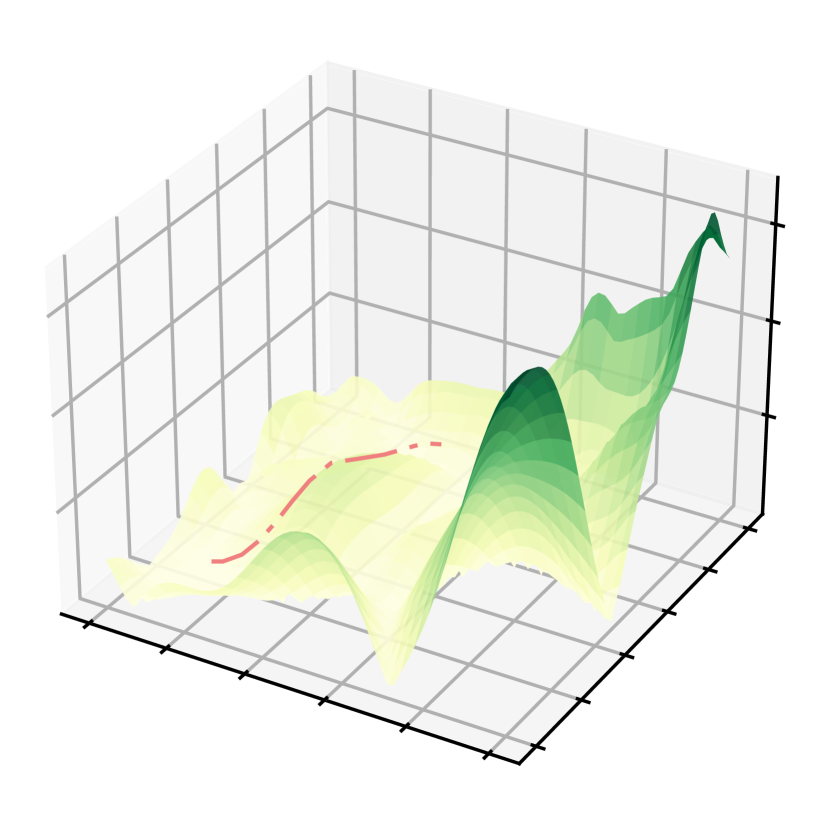
(a) $|f({\bm{x}}^{+};{\bm{\theta}})|$

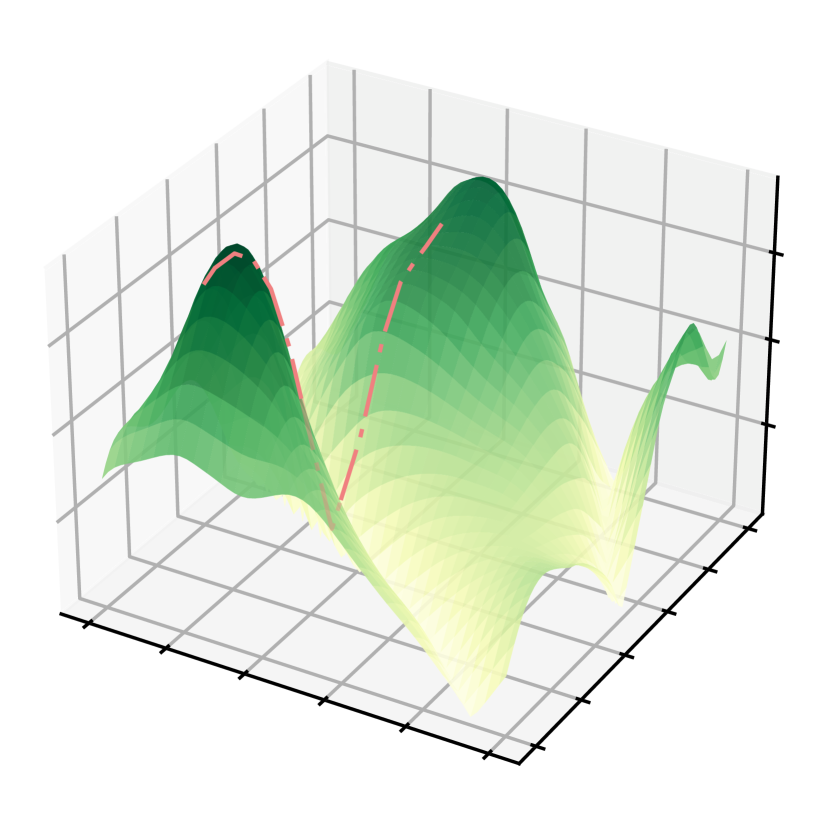
(b) $|f({\bm{x}}^{-};{\bm{\theta}})|$

Figure 2: The loss landscape $|f({\bm{x}};{\bm{\theta}}(u,v))|$ evaluated on a true surface point ${\bm{x}}^{+}$ and a false-positive point ${\bm{x}}^{-}$. The pink dotted lines indicate the actual loss variation along the continually learned ${\bm{\theta}}^{1:T}$. It is clear that the landscape of the true surface point stays in a low-loss basin, while that of the false-positive point falls along a sharp ridge that reaches the low-loss valley once.

As noticed in Sec. 3, central to our method is the identification of the next target view that brings a significant distribution shift $\delta{\bm{z}}^{*}$. A local planner is then deployed as a generalization maximizer that decides the following agent movement ${\bm{a}}^{t:t+k}$ to the target location and captures the corresponding data. Given the locally upper-bounded $H(\delta{\bm{z}}^{*},{\bm{\theta}}^{t})$, the map parameters are optimized with the new observation, thus achieving a local equilibrium point of $H(\delta{\bm{z}}^{*},{\bm{\theta}}^{*})$. The process is iteratively conducted that drives the mobile agent to actively explore the environment. In this section, we begin with an empirical analysis of how $\delta{\bm{z}}^{*}$ can be found. The implementation of the active neural mapping system is introduced afterward.

4.1 Through the lens of loss landscape

Eq. 3 motivates us to understand the behavior of the loss $L({\bm{\theta}},{\bm{z}})$ during continual learning: the equilibrium point of $\{\delta{\bm{z}}^{*},{\bm{\theta}}^{*}\}$ indicates the requirement of a flat low-loss landscape for surface points to avoid forgetting (the minimization of the first and third terms in Eq. 3) and an evident loss discrepancy for finding $\delta{\bm{z}}$ so the generalization is maximized. Following [37, 72], we define a hyperplane by two orthonormal vectors $\{{\bm{u}},{\bm{v}}\}$, where any sample ${\bm{\theta}}$ in the weight space can be represented by the linear combination of the two vectors as ${\bm{\theta}}(u,v)=u{\bm{u}}+v{\bm{v}}$. We can then estimate the prediction $f({\bm{x}};{\bm{\theta}}(u,v))$ given any queried location ${\bm{x}}$ through a single forward pass and obtain the magnitude of the loss landscape $L({\bm{\theta}},{\bm{z}})$.

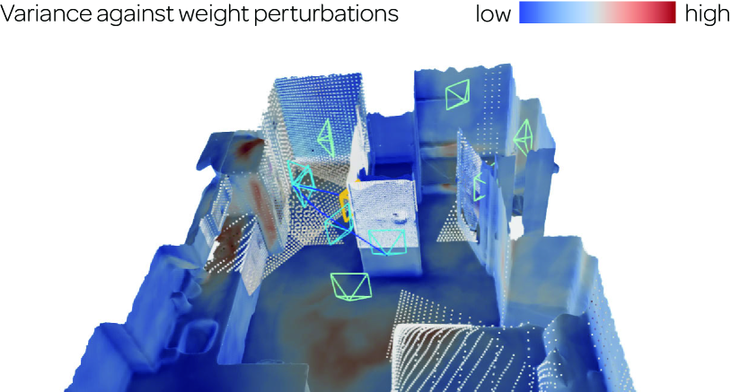
Figure 3: The functionality changes due to weight perturbations given the ground truth surface points ${\bm{x}}\in{\mathcal{D}}$. It can be noted that most high-variance regions (with warm colors) locate near the boundaries of space between explored (colored point cloud) and unexplored areas.

We randomly pick a true surface point ${\bm{x}}^{+}$ observed at $t=1$ and a false-positive zero-crossing point ${\bm{x}}^{-}$ generated at $t=200$ due to the continuous nature of the neural map. The prediction over the entire weight space is then calculated through forward passes given ${\bm{\theta}}(u,v)$. As presented in Fig. 2, by projecting the high-dimensional weight space onto the hyperplane, we can easily visualize the loss changes along the optimization path. Empirically, we observe evidently-different geometries for the true surface point and the false-positive one: the loss of the true surface point will be constrained in a low-loss basin, while the loss of the false-positive one stays along a sharp ridge that once jumps over a high-loss ridge into the valley at $t=200$ and then keeps ascending.

The reason behind this phenomenon is straightforward. During continual learning, the parameters of the neural map undergo constant changes. The functionality of $f({\bm{x}};{\bm{\theta}}^{t})$ will only remain stable in previously-observed areas with constant self-supervision (as verified in [78, 69, 47] through a simple experience replay strategy). In not-well-explored areas, the functionality can easily change due to a lack of constraints. That is to say, the neural map is more susceptible to areas where the functionality changes the most against parameter perturbations:

$${\bm{x}}=\arg\max\mathbb{V}_{\hat{{\bm{\theta}}}\sim\mathit{N}({\bm{\theta}},b^{2}\mathit{I})}[f(\mathbf{x};\hat{{\bm{\theta}}})].$$ (4)

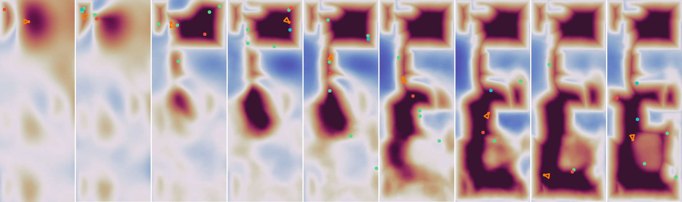
Figure 4: The evolution of the learned signed distance field through active neural mapping in 1000 steps. The proposed system is conducted in a receding horizon fashion. The target locations (green dots) are constantly pushed to the not-well-explored or not-well-trained regions for reaching a local equilibrium point. See the supplementary video for better visualization.

The term in Eq. 4 is referred to as the artificial neural variability [76] that shares similar concepts with the neural variability in neuroscience [46, 39, 21]: neuronal activity fluctuates over time given the same inputs, indicating the uncertainty of perceptual inference. By evaluating the prediction variability given points on the zero-crossing surfaces through weight perturbation, the false-positive ones and the true-positive ones can be evidently distinguished due to variable behaviors, and observations around the false-positive ones indicate high generalization cost (the second term of Eq. 3) as they land in sharp and unstable minima.

As illustrated in Fig. 3, the functional sensitivity of Eq. 4 is directly linked with the data distribution of past observations that supervise the neural map, and explicitly indicates the prediction quality and uncertainty. High-variance regions are usually around the boundaries of space between explored and unexplored areas (where false-positive zero-crossing surfaces are generated). This is in common with the prevalent concept of the frontier. The differences lie in that the high-variance regions are naturally indicated by the neural map in a data-driven fashion instead of the heuristic design. Besides, unlike frontiers that rely mainly on adjacent occupancy status, regions with scarce data or with thin structures may also fall into a high-variance region in our case as they struggle to converge. Hence, all areas that are not accurately represented are taken into account. We refer readers to the supplementary video for a better understanding.

4.2 An online active neural mapping system

In this paper, we target a continuous signed distance function (SDF) of $f({\bm{x}};{\bm{\theta}}):{\mathbb{R}}^{3}\to{\mathbb{R}}$ as the scene geometry representation, where the neural map ${\bm{\theta}}$ is continually optimized and guides the mobile agent to not-well-explored areas. The system is implemented as four steps: 1) identifying the target viewpoints; 2) selecting the best target viewpoint; 3) navigating to the target location; 4) and optimizing the neural map parameters given newly-captured data.

The target view identification serves as finding the most distribution shift $\delta{\bm{z}}^{*}$. A zero-mean Gaussian perturbation around the instant map parameters ${\bm{\theta}}^{t}$ is performed every time a keyframe is selected, where the variance $\mathit{I}$ is set as the norm of recent parameter changes $|{\bm{\theta}}^{t}-{\bm{\theta}}^{t-1}|$. We sample points on the predicted zero-crossing surface to distinguish between the real surface points and the false-positive ones. This is close in spirit to the frontier-based method in a sample-based fashion. In practice, the top 10% points with the highest variance $\mathbb{V}_{\hat{{\bm{\theta}}}\sim\mathit{N}({\bm{\theta}},b^{2}\mathit{I})}[f(\mathbf{x};\hat{{\bm{\theta}}})]$ are selected and then clustered based on the geometrical similarity. To make the selected samples in sight, we place the target locations (green dots in Fig. 4) at a fixed distance along the surface normal $\nabla f({\bm{x}};{\bm{\theta}}^{t})$, where the continuous and differentiable neural representation allows for convenient gradient computation through auto-differentiation. To determine the best view (the red dot in Fig. 4) among the target location candidates, we evaluate each cluster with three criteria: the maximum variance against parameter perturbations, the number of points within the cluster, and the distance between the cluster center and the current agent position. As illustrated in Fig. 4, the red dot and cyan dot are selected based on different criteria. Besides, a local planning horizon [8, 84, 6] is adopted that prioritizes the target viewpoint candidates within the frustum bounding box. Therefore, the agent (the orange arrow in Fig. 4) will choose the best candidate in sight as the target view.

Within each receding horizon loop $[t,t+k]$, the point-goal navigation for deciding the agent actions ${\bm{a}}^{t:t+k}$ and the continual learning for updating the map parameters ${\bm{\theta}}^{t:t+k}$ are exactly the optimization process for maximizing generalization and minimizing forgetting, indicating the dynamics of ${\bm{a}}$ and ${\bm{\theta}}$ to reach the equilibrium point of $\{\delta{\bm{z}}^{*},{\bm{\theta}}^{*}\}$ within a local horizon. For point-goal navigation, we adopt the reinforcement-learning-based DD-PPO [74] to reach the next target viewpoint. For incrementally updating the neural map, we adopt the experience-replay-based strategy of iSDF [47] with similar architecture and loss functions. It should be noted that other planner [2, 33, 36] and continual learning strategies [78, 69] can be naturally incorporated as optimizers that decide the optimization path to reach the local equilibrium point of $\delta^{*}$ and ${\bm{\theta}}^{*}$.

5 Experiments

Central to the paper is a novel target view identification module through weight perturbations and an online active mapping system with a 3D implicit neural representation. In this section, we evaluate the performance of the system through comprehensive experiments.

5.1 Experimental Setup

The experiments are conducted on a desktop PC with an Intel Core i7-8700 (12 cores @ 3.2 GHz), 32GB of RAM, and a single NVIDIA GeForce RTX 2080Ti.

Data acquisition. Our algorithm is conducted with the Habitat simulator [58] and evaluated on the visually-realistic Gibson [75] and Matterport3D datasets [9]. The experiments are conducted in 1000/2000 steps depending on the scene scale. The system takes posed depth images at the resolution of $256\times 256$ as inputs and outputs discrete action at each step. The action space consists of MOVE_FORWARD by $6.5$$cm$, TURN_LEFT and TURN_RIGHT by $10^{\circ}$, and STOP. The mobile agent is randomly initialized in the traversable space at the height of $1.25$m. The field of view (FOV) is set to $90^{\circ}$ vertically and horizontally.

Neural map architecture. Our neural map is a single multi-layer perceptron (MLP) with 4 hidden layers and 256 units per layer. Following [47], a softplus activation and a positional embedding are adopted, where the positional embedding is concatenated to the third layer of the network. The neural map is optimized using the Adam optimizer with a learning rate of $0.0013$.

5.2 Evaluation metrics

We adopt the following metrics for evaluating the incrementally-updated neural map:

MAD ($cm$). The mean absolute distance is evaluated by estimating the distance prediction through a forward pass on all vertices from the ground truth mesh. This metric defines the accuracy of the learned 3D neural distance field.

FPR (%). The false-positive rate is calculated as the percentage of samples from the reconstructed mesh whose nearest distance to the ground truth mesh exceeds $5$$cm$. This metric defines the quality of the mesh extracted from the 3D continuous neural map.

Comp.. The completeness metrics are calculated from the ground truth vertices to the entire observations that are actively captured. By estimating per-vertex nearest distance to the past observations ${\bm{z}}^{1:t}$, the percentage of points whose nearest distance is within 5cm (Comp. (%)) and the mean nearest distance (Comp. ($cm$)) can be calculated to measure the active exploration coverage in 3D space.

5.3 Comparisons against other methods

Table 1: The coverage of the actively-captured data. See supplementary material for results on each scene for details.

	Gibson		MP3D
	Comp. ↑	Comp. ↓	Comp. ↑	Comp. ↓
	(%)	($cm$)	(%)	($cm$)
Random	45.80	34.48	45.67	26.53
FBE	68.91	14.42	71.18	9.78
UPEN	63.30	21.09	69.06	10.60
OccAnt	61.88	23.25	71.72	9.40
Ours	80.45	7.44	73.15	9.11

We compare the proposed method against three relevant methods: FBE [77] aims to push the boundaries between unknown and known space for exploration; OccAnt [57] anticipates the occupancy status in unseen areas and rewards the agent with accurate anticipation; UPEN [24] tries to select the most uncertain path via the ensemble of occupancy prediction models. As the three methods utilize the 2D grid-based map representation, we evaluate the completeness of the actively-captured observations along the trajectory using the Comp. (%) and the Comp. ($cm$) metrics.

As presented in Tab. 1, the proposed active mapping system consistently outperforms the three competitors. It should be noted that FBE and UPEN adopt the same DD-PPO planner as ours for target goal navigation. Therefore, the efficacy of the proposed goal location identification strategy can be fairly evaluated. FBE relies purely on the voxel-based geometric information for identifying the frontiers, whereas the selection mechanism is manually designed that can easily ignore areas that have been explored with insufficient data. In contrast, the proposed method well quantifies the map uncertainty to achieve better performance. In terms of OccAnt, the agent occasionally moves back and forth as the goal location identification is trained through a rewarded mechanism, while the proposed goal location identification strategy and the local planning horizon guarantee stable exploration routes. UPEN adopts a deep ensemble based manner [34] to quantify the prediction uncertainty, which shares a similar idea with the proposed method regarding epistemic uncertainty reasoning. Nevertheless, UPEN simply generates multiple traversable path candidates towards a pre-defined unreachable goal location with a global RRT planner, where the map uncertainty merely ranks the path candidates to achieve the best information gain, while the proposed method better explores the environment by explicitly exploiting the neural variability for goal location identification and selection.

5.4 Ablation study and system performance

Table 2: Ablation study of the map quality regarding the SDF prediction (MAD), the reconstructed mesh (FPR), and the observation completeness (Comp.).

		MAD ↓	FPR ↓	Comp. ↑
		($cm$)	(%)	(%)
	Random	8.49	36.57	45.80
Gibson	Module 1	5.68	34.65	79.48
	Module 3	5.44	25.09	76.19
	Module 4	6.11	32.86	73.70
	Ours	5.10	28.04	80.45
	Random	8.87	51.88	45.67
MP3D	Module 1	4.65	43.03	71.41
	Module 3	6.06	39.05	74.63
	Module 4	4.30	47.99	67.75
	Ours	4.29	40.07	73.15

As mentioned in Sec. 4.2, the proposed active neural mapping system allows drop-in substitutes to replace the existing modules. We provide detailed ablation studies to justify the reasonable design of each module.

Module 1: target view identification. We replace the proposed weight perturbation module with MC-Dropout [22] (p=0.05) and a BALD [29] score to quantify the prediction uncertainty. The output is sampled five times in our experiments. As demonstrated in Tab. 2, the proposed goal location identification strategy achieves better results compared to the substitute. Although the uncertainty quantification method leads to comparable exploration efficiency, the involvement of Dropout layers leads to noisy and coarse geometry and inefficient inference.

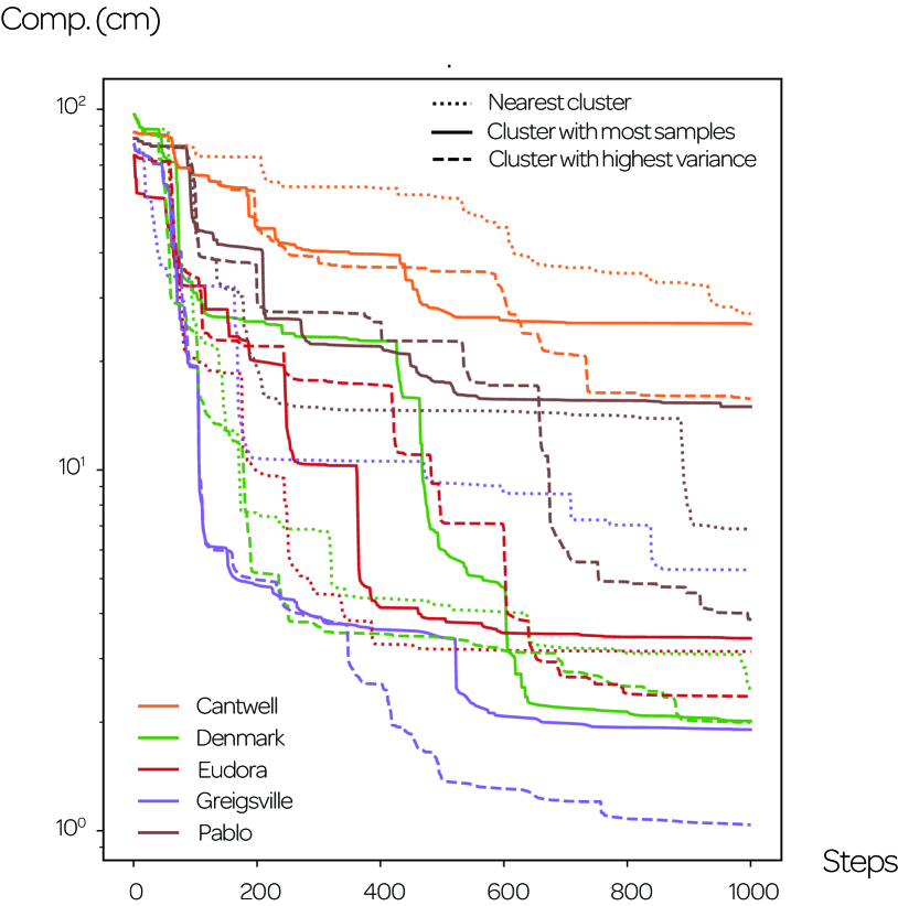
Figure 5: The effect of different candidate selection criteria (Module 2) on the Comp. ($cm$) ↓ metric in 1000 steps. Best viewed in color to see results on different scenes.

Module 2: best candidate selection. As illustrated in Fig. 5, we evaluate the performance of the three different selection criteria mentioned in Sec. 4.2. Results on different scenes share a similar conclusion: selecting the highest variance regions will lead to the best performance. This result meets the arguments in Sec. 3 and 4 to obtain the equilibrium point by maximizing generalization, or in other words, moving to the highest variance areas as Eq. 4.

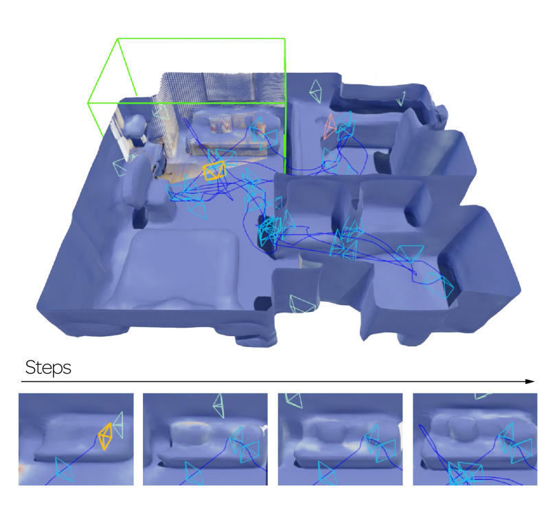
Figure 6: Continual learning of the scene geometry.

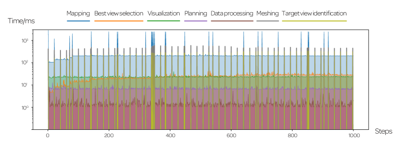
Figure 7: The runtime for each module. The impulse of the runtime is caused by a keyframe-based or windowed execution.

Module 3: local planner. In our final setting (Ours) and for evaluating FBE/UPEN, we choose the DD-PPO⁺ model trained on Gibson4+ and Matterport3D (train/val/test) for evaluating the Gibson validation sequences, and choose the DD-PPO^⋆ model trained on Gibson2+ for evaluating the Matterport3D test sets to avoid the over-fitting issue. We here alter the model choice to further evaluate the performance on Gibson with the DD-PPO^⋆ and on Matterport3D with DD-PPO⁺. Without pretrained data from Matterport3D, DD-PPO^⋆ results in degradation on large scenes and improvement in small ones, while DD-PPO⁺ leads to more robust and balanced results. We refer readers to the supplementary material for a more detailed per-scene analysis. The results further verify the efficacy of the proposed goal location identification strategy: a more powerful planner will bring better exploration results only if the goal location is properly decided.

Module 4: learning of the neural map. Different network architectures affect the convergence rate and the generation of false-positive zero-crossing surfaces. We further evaluate the active neural mapping system with a different network architecture: a single MLP with positional encoding [44] and ReLU activations. As the substitute architecture converges slower for high-frequency components [71], the reconstruction accuracy deteriorates compared to our final setting (Ours). Meanwhile, the exploration is slightly affected as the prediction in visited areas may still be inaccurate. Nevertheless, the system still works effectively given a different network architecture, suggesting the applicability to embracing the latest advances in implicit neural representations.

System performance. In general, our system achieves promising reconstruction accuracy and completeness given limited steps. The computational cost for each module is illustrated in Fig. 7, where the runtime per step is 0.33s on average. The system is real-time capable and can be accelerated by reducing the per-frame iteration during continual learning. As illustrated in Fig. 6, the prediction of scene geometry over previously seen areas is continually improved during exploration, and the coverage of space continues to grow. The continual learning fashion allows for constant map optimization and lifelong learning of the scene.

6 Conclusion

In this paper, we introduce a novel active mapping system based on implicit neural representations. The key to the solution is a goal location identification strategy through weight perturbation that drives the mobile agent to the areas with the most distribution discrepancy. The active mapping is achieved by alternatively performing action decisions to reach the goal location, and map parameter updating given incoming observations. The iterative process can be viewed as a joint optimization to reach an equilibrium point within the receding local horizon, guaranteeing a promising scene geometry recovery through autonomous exploration. The proposed strategy and the overall design of the system are justified through experiments and ablation studies.

6.1 Limitations and future potentials

Though the weight perturbation provides a convenient way to find the next best view, the action decision of the system is dependent on the map-free local planner, which may occasionally get stuck by objects out of view or in narrow areas. Better exploiting the information inherited in the neural map for online navigation and replanning is one natural extension of the proposed system. Possible solutions include optimization-based planners [2, 33] and INR-guided reinforcement learning to replace the existing planner trained with a 2D top-down map or raw observations. Meanwhile, the target view selection module simply discards other goal location candidates. Without exploiting temporal and historical cues, the agent may move back to visited areas where the complicated geometry is hard to converge. This issue may be handled by a graph model [79] for candidate organization and assignment or a decomposed and hierarchical representation for object-wise or room-wise exploration.

Enabling the mobile agent to behave autonomously in an unknown space is one straight path towards spatial intelligence [16, 17]. The implicit neural representation has shown great potential to distill knowledge from pre-trained model [61, 53] for a globally consistent and informative representation. Best exploiting the information inherited in the prior and streaming data to construct a decodable and task-agnostic scene representation may lead to an innovative map-centric paradigm for the vision, graphics, and robotics communities.

Acknowledgements

We thank anonymous reviewers for their fruitful comments and suggestions. This work is supported by the Joint Funds of the National Natural Science Foundation of China (U22A2061) and National Natural Science Foundation of China (62176010).

Supplementary Materials

I Runtime

Supplementary to Fig. 7 of the main paper, we estimate the average portion of the computational cost induced by each module in Fig. S1. The majority of the runtime is distributed to the continual learning of the neural map (71%), while best view selection and identification, visualization, and meshing take most of the rest computational resources.

II Discussion on uncertainty quantification

We refer readers to [1] for a more comprehensive review of uncertainty quantification methods. For active mapping, we are interested in the epistemic uncertainty that characterizes the incomplete knowledge of ${\mathcal{D}}$ given existing training samples. In the field of implicit neural representation and learning-based active mapping, a few uncertainty quantification methods are adopted, e.g., variational inference [64, 62], distribution analysis of the output space [36, 48], or ensemble technique [24, 70]. Variational inference based approaches reformulate the architecture and the training process, hence limiting its application to existing neural representations. Ensemble methods require random initialization for each ensemble to induce prediction variance, which is impractical for our continual learning setting. In contrast to the distribution analysis of the output space, we examine the parameter space of the implicit neural representations and formulate active mapping from a continual learning perspective. The proposed method is simple and can be easily applied to different architectures and training paradigms. The proposed problem setting is also similar to Bayesian active learning [23]. Hence, we also adopt the MC-Dropout layers with a BALD score as the substitute for Module 1. Compared to the proposed method, the involvement of Dropout leads to slow inference as a single forward pass leads to noisy prediction. Even though the exploration efficiency is comparable (Tab. S4), the reconstructed mesh from averaged SDF prediction is still noisy (Fig. 4(a)) even after 5 runs. Note that most modules with 98% of the computational time in Fig. S1 require a noise-free prediction. Increasing the number of feedforward passes would be computationally burdensome for an online system.

Figure S1: The runtime distribution of each module.

III More experimental results

In this section, more results on the Gibson [75] and Matterport3D datasets [9] are provided as supplementary evaluations to Tab. 1 and 2 of the main paper.

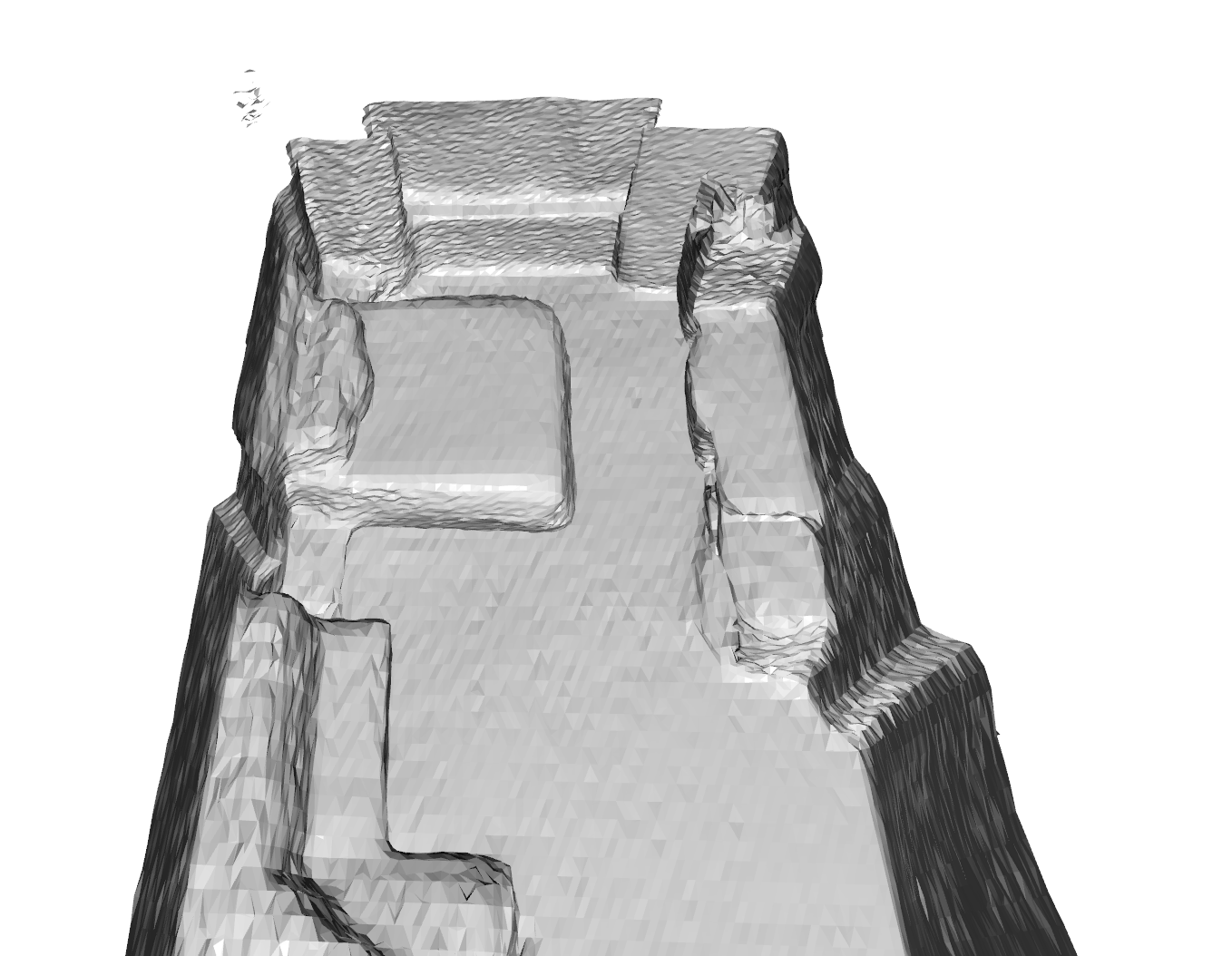
(a) Module 1 (Dropout)

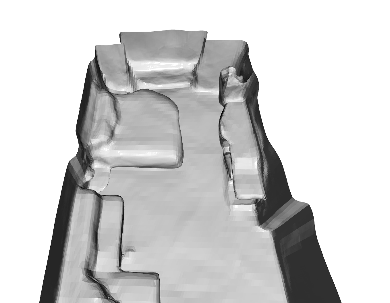
(b) Module 3 (ReLU)

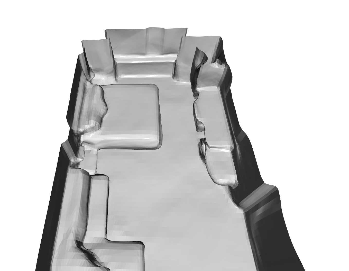
(c) Final

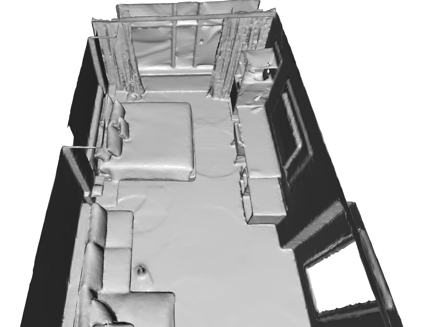
(d) GT

Figure S2: Extracted meshes from different baselines.

III.1 Per-scene evaluation

We conduct experiments on single-floor scenes with less than 10 rooms. Scenes in Matterport3D are consistently larger and more complex than in Gibson (see the number of keyframes (Kfs) in Tab. S1). The keyframes are automatically selected as frames with high prediction losses. Both a large scene that requires a long trajectory for exploration and a complex scene that can not be easily recovered lead to a large number of keyframes, hence indicating the scene complexity. For small scenes (num_room $<=$ 5), the active mapping is conducted in 1000 steps; While for large scenes (num_room $>$ 5), we run 2000 steps for better coverage. $<$ 5cm (%) is defined as the ratio of ground truth mesh vertices whose predicted distance value is within 5cm. Acc. is defined as the mesh-wise mean distance between the estimated one and the ground truth.

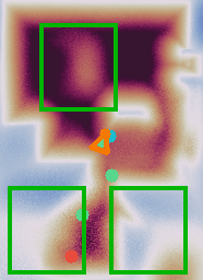
(a) Module 1

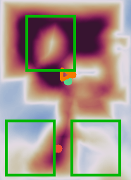
(b) Module 3

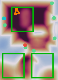
(c) Final

Figure S3: Learned SDF from different baselines.

From the per-scene evaluation, we can obtain a better understanding of the proposed method. When comparing to the relevant methods in Tab. S1, we can find a typical failure case of HxpkQ, which will be further explained in Sec. III.2. The major reason for the failure is the local planner that gets stuck in the narrow area. Meanwhile, the evaluations on different module substitutes in Tab. S2-S4 uncover several important insights:

$\bullet$ Trade-offs between mapping accuracy and area coverage. As a surface-based exploration method, the choice of different network architectures and penalty functions may lead to diverse performance. For instance, the ReLU activations without skip-connection lead to inferior accuracy in high-frequency areas (see Fig. 2(b)), hence the target view identification module may guide the agent to visited areas as the high-frequency geometric details are not recovered well. Consequently, the mesh quality and the exploration completeness decline (See Tab. S3 and S4).

Table S1: Comparison against relevant methods regarding the completeness of actively-captured observations.

			Comp. (%) ↑
	Rooms	Kfs	Random	FBE	UPEN	OccAnt	Ours
Gibson-Cantwell*	8	38	24.43	40.93	39.42	37.96	61.36
Gibson-Denmark	2	18	27.83	70.28	66.41	65.07	85.86
Gibson-Eastville*	6	34	14.32	58.49	51.51	27.03	74.21
Gibson-Elmira	3	14	66.29	72.69	82.14	84.37	91.65
Gibson-Eudora	3	13	53.89	76.65	75.74	74.07	90.12
Gibson-Greigsville	2	23	75.44	90.34	73.72	88.27	92.47
Gibson-Pablo	4	14	46.87	76.06	54.16	64.50	72.88
Gibson-Ribera	3	14	44.29	79.26	81.21	66.97	88.62
Gibson-Swormville*	7	31	58.81	55.46	45.43	48.64	66.86
Gibson-mean	4	22	45.80	68.30	63.30	61.88	80.45
MP3D-GdvgF*	6	32	68.45	81.78	82.39	80.24	80.99
MP3D-gZ6f7	1	48	29.81	81.01	82.96	82.02	80.68
MP3D-HxpKQ*	8	32	46.93	58.71	52.70	60.50	48.34
MP3D-pLe4w	2	52	32.92	66.09	66.76	67.13	76.41
MP3D-YmJkq	4	68	50.26	68.32	60.47	68.70	79.35
MP3D-mean	4	46	45.67	68.53	69.09	71.72	73.15

	Comp. (cm)↓
Random	FBE ↑	UPEN	OccAnt	Ours
59.59	37.03	42.12	43.27	17.67
50.42	12.40	17.34	16.96	3.78
72.39	24.08	28.16	60.67	11.36
11.63	10.40	5.35	4.35	2.57
23.24	8.11	9.18	9.27	2.27
6.97	2.62	16.34	3.25	1.78
34.70	6.38	31.81	20.49	9.96
33.27	6.53	5.74	18.67	4.13
18.10	22.19	33.78	32.34	13.43
34.48	14.42	21.09	23.25	7.44
11.67	5.48	5.14	5.66	5.69
46.48	7.06	6.14	6.19	7.43
19.10	11.75	14.11	11.75	15.96
30.79	12.78	11.82	11.51	8.03
24.61	11.85	15.77	11.90	8.46
26.53	9.78	10.60	9.40	9.11

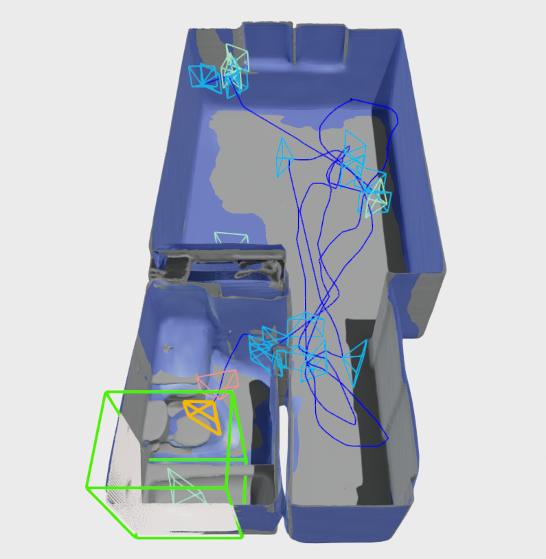
(a) Edgemere

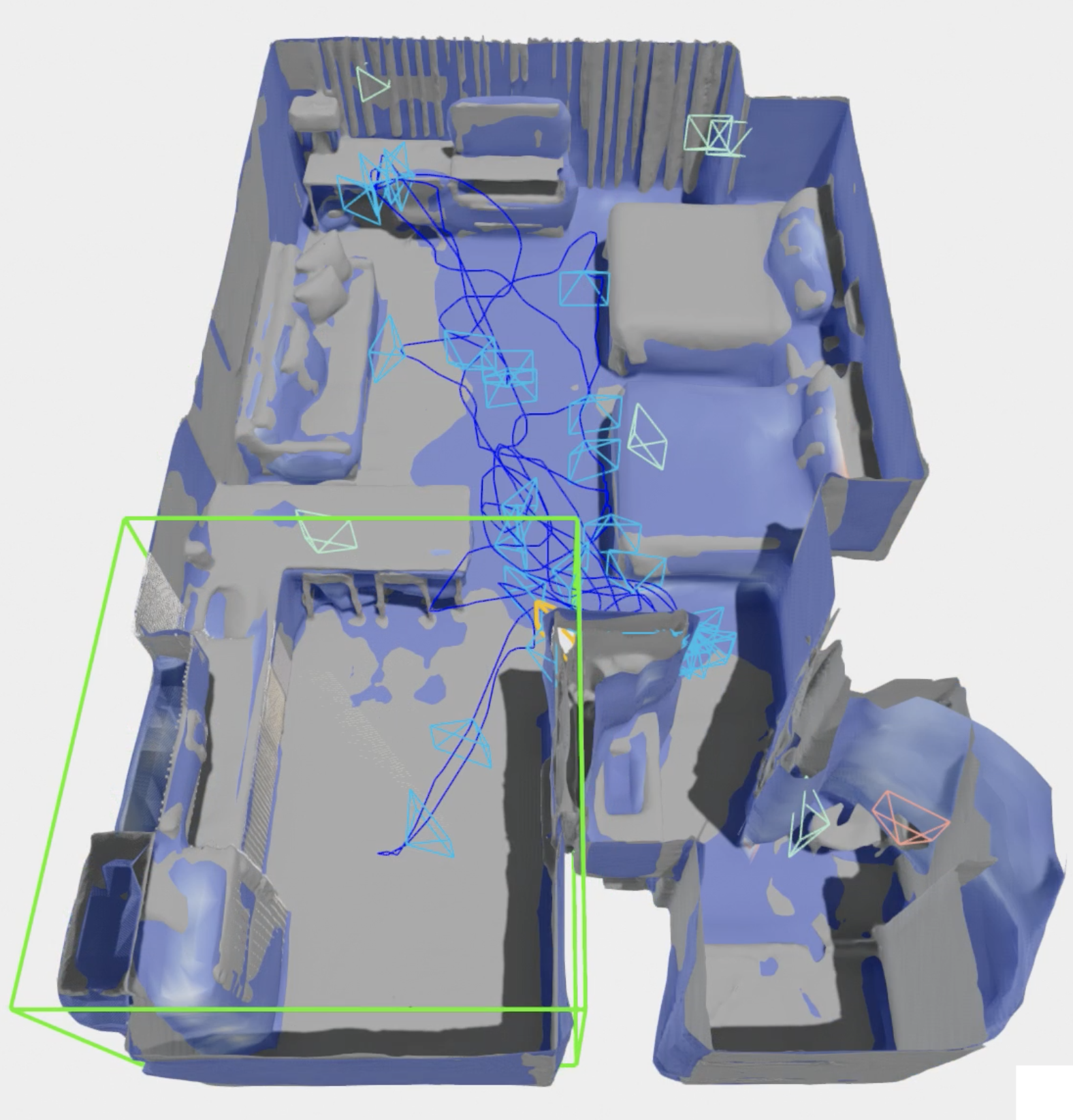
(b) Elmira

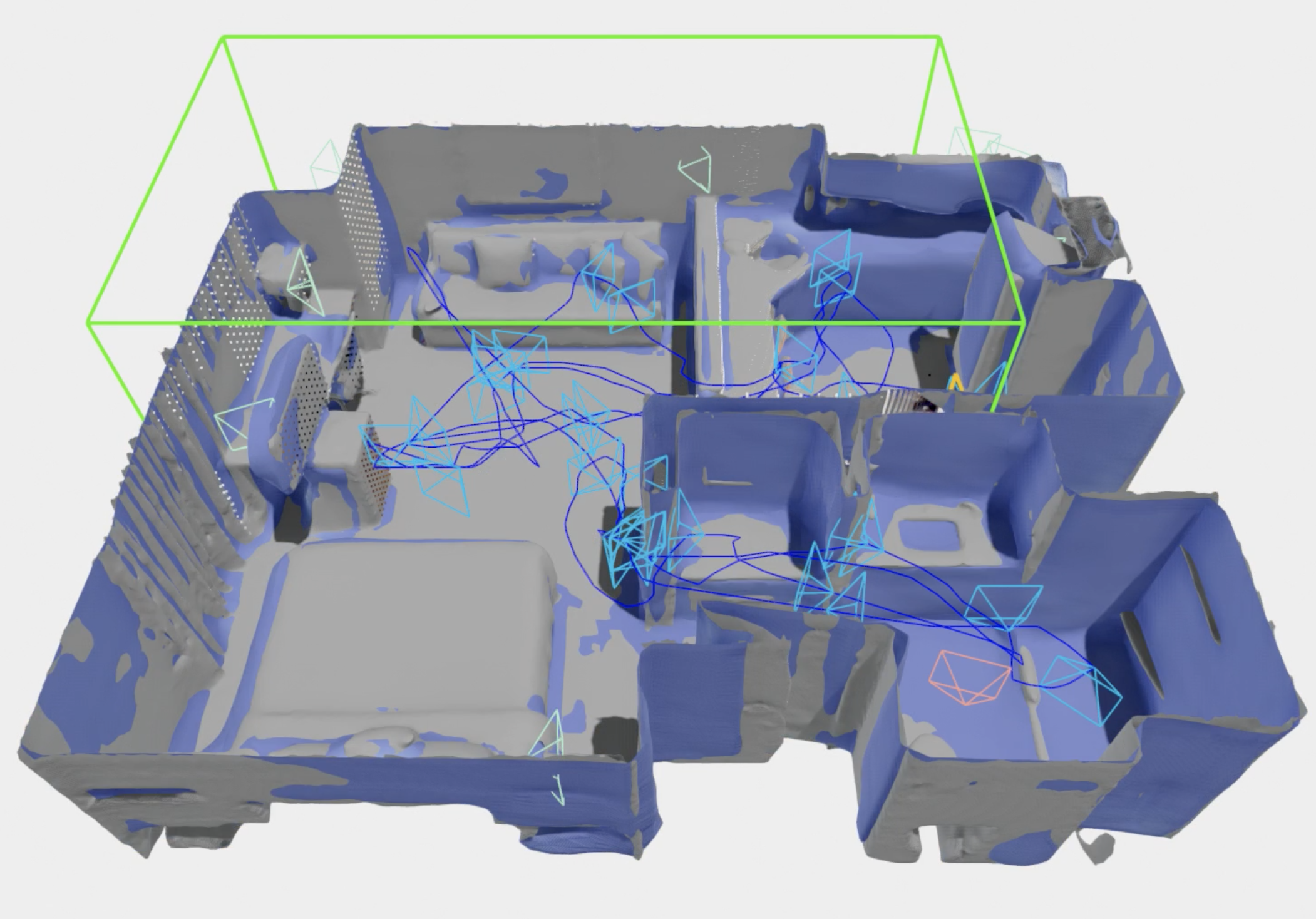
(c) Eudora

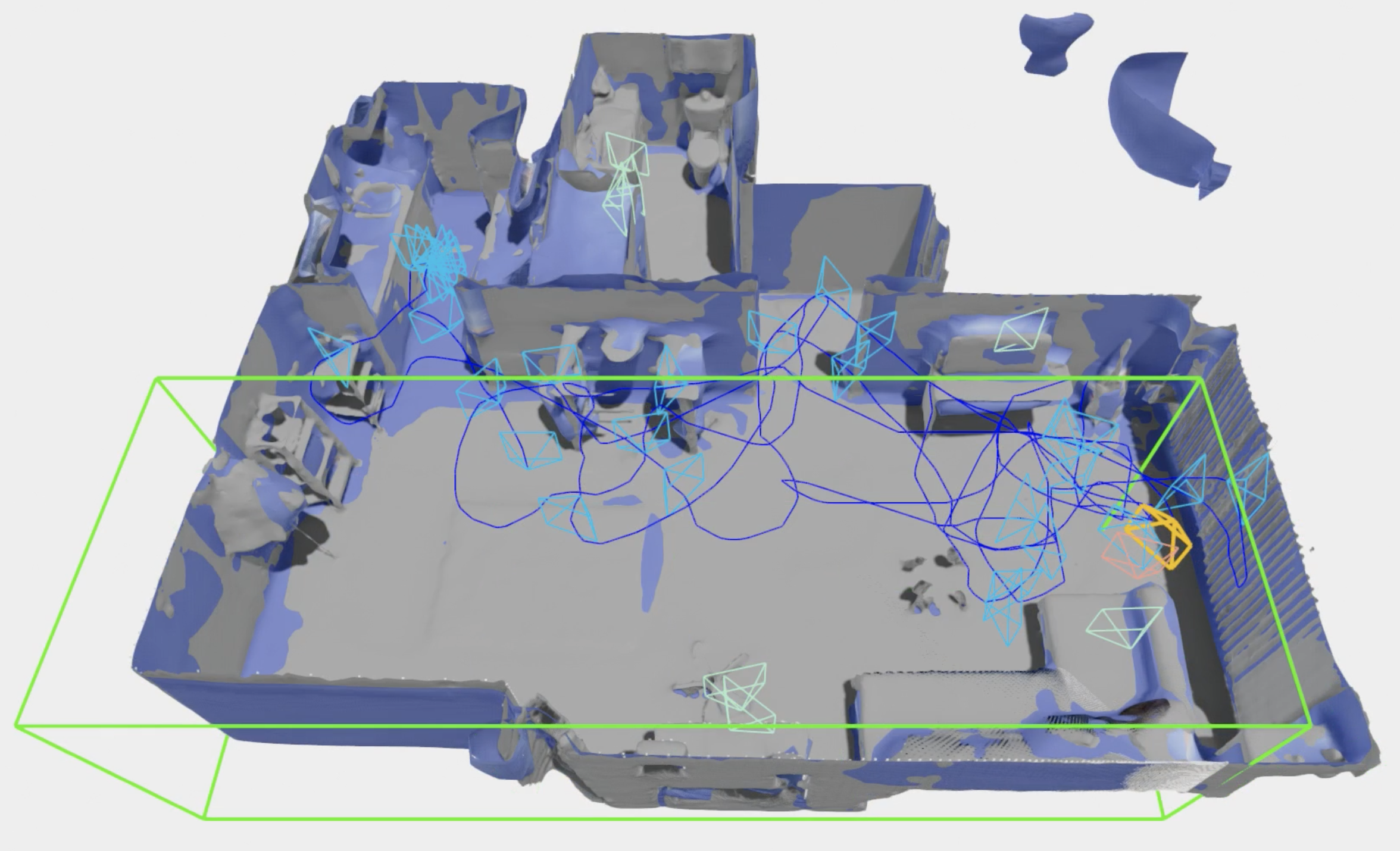
(d) Greigsville

Figure S4: Examples of well-explored scenes. The ground truth mesh is in grey while the estimated one is in blue.

(a) Gibson-Swormville

(b) MP3D-HxpKQ

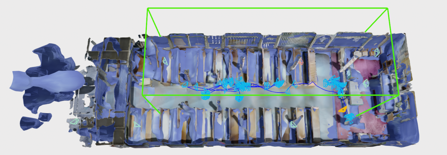
(c) MP3D-YmJkq

Figure S5: Typical challenges: (a) low $<$5cm(%) due to incomplete exploration; (b) low Comp. as the agent gets stuck; (c) high FPR due to extreme occlusions.

$\bullet$ Generalization ability matters. Meanwhile, there are also different prediction behaviors in unobserved areas when deployed under different architectures/penalties, leading to different generalization abilities. As illustrated in Fig. S3, the predicted distance values in unexplored areas (within the green bounding box) are smaller for module 3 baseline (PosEnc+ReLU) than the module 1 (PosEnc+SoftPlus+Dropout) and final baselines (PosEnc+SoftPlus). This may affect the generation of false-positive zero-crossing surfaces and the convergence rate when new data come, thus affecting the active mapping performance. That’s also the reason why module 4 achieves higher $<$5cm (%) in Tab. S2 even if it explores fewer areas (Tab. S4) with a worse mesh model (Tab. S3).

III.2 Limitations and typical challenges

As illustrated in Fig. S4, the proposed method can recover high-fidelity scene geometry through autonomous exploration. All rooms are well-explored, thus achieving high Comp. in Tab. S1. Compared to other baselines, the proposed method achieves much better coverage. It should be noted that the Comp. metrics are only affected by the action (trajectory). The results clearly verify the efficacy of the proposed method.

We here emphasize the typical challenges that lead to unsatisfactory results. As illustrated in Fig. 5(a), the bad SDF prediction results mainly contribute to incomplete exploration. On the other hand, the mesh quality is highly relevant to the complexity of the scene geometry. As illustrated in Fig. 5(c), although a straight path leads to efficient exploration, the church scenario is full of occlusions that make accurate reconstruction non-trivial. Finally, as illustrated in Fig. 5(b), as the agent gets stuck all the time, all metrics are unpleasant for HxpKQ even if the environment is open without occlusions.

We can also find that the major reason for the failure cases is the unsatisfactory trajectory/navigation. Even though target location candidates exist in the unexplored rooms (see Fig. 5(a)), entering a narrow door/corridor or even going upstairs brings little information gain sometimes due to a limited field of view. If the agent gets stuck easily in nearby areas, the target candidate may never be chosen as the optimal one. For future extensions, better local planning strategies should be deployed to handle the challenges as discussed in Sec. 6.1 of the main paper.

Table S2: Comparison against baselines regarding the SDF prediction accuracy of the zero-crossing surface.

			MAD (cm) ↓
	Rooms	Kfs	Random	Module 1	Module 3	Module 4	Final
Gibson-Cantwell*	8	38	8.83	6.10	8.12	8.28	5.20
Gibson-Denmark	2	18	9.06	4.59	4.74	4.92	4.32
Gibson-Eastville*	6	34	16.66	6.65	5.19	6.96	6.64
Gibson-Elmira	3	14	4.72	5.01	3.89	3.89	4.01
Gibson-Eudora	3	13	8.03	4.22	4.62	7.08	4.02
Gibson-Greigsville	2	23	4.55	4.10	4.35	3.87	4.18
Gibson-Pablo	4	14	7.48	4.87	6.66	7.96	5.23
Gibson-Ribera	3	14	6.29	5.27	4.95	5.79	5.13
Gibson-Swormville*	7	31	10.80	10.29	6.46	6.22	7.17
Gibson-mean	4	22	8.49	5.68	5.42	6.10	5.10
MP3D-GdvgF*	6	32	6.78	6.67	7.53	5.97	3.77
MP3D-gZ6f7	1	48	23.12	4.12	5.37	4.46	3.18
MP3D-HxpKQ*	8	32	4.60	5.69	7.31	4.99	7.03
MP3D-pLe4w	2	52	6.22	3.14	4.48	2.83	3.25
MP3D-YmJkq	4	68	3.65	3.61	5.60	3.25	4.22
MP3D-mean	4	46	8.87	4.65	6.06	4.30	4.29

	$<$5cm (%) ↑
Random	Module 1	Module 3	Module 4	Final
39.07	51.23	46.52	45.95	59.93
45.68	68.47	66.98	65.22	70.14
15.50	46.72	56.95	42.95	51.33
64.65	63.04	70.84	71.42	72.27
51.20	66.48	66.88	55.68	71.98
66.52	71.61	68.38	71.10	74.95
50.49	62.16	45.36	55.35	60.41
59.59	58.42	63.51	58.66	65.37
28.40	32.60	49.16	53.29	44.16
46.79	57.86	59.40	57.74	63.39
67.27	70.23	63.39	76.74	77.05
28.01	77.59	64.42	75.42	75.03
67.80	61.47	49.52	66.97	53.72
63.60	78.79	64.47	82.78	75.22
72.44	74.59	55.56	82.12	72.67
59.82	72.53	59.47	76.81	70.74

Table S3: Comparison against baselines regarding the reconstructed mesh quality.

			FPR (%) ↓
	Rooms	Kfs	Random	Module 1	Module 3	Module 4	Final
Gibson-Cantwell*	8	38	51.32	60.80	37.37	51.95	45.41
Gibson-Denmark	2	18	40.43	17.13	15.83	22.96	22.31
Gibson-Eastville*	6	34	68.04	54.89	44.86	61.70	46.33
Gibson-Elmira	3	14	25.02	33.54	16.71	24.54	15.94
Gibson-Eudora	3	13	22.47	17.69	17.56	23.57	18.06
Gibson-Greigsville	2	23	26.63	27.80	24.18	26.12	23.07
Gibson-Pablo	4	14	28.82	24.43	21.99	20.31	22.51
Gibson-Ribera	3	14	27.25	20.53	23.08	28.88	34.51
Gibson-Swormville*	7	31	39.17	55.04	24.21	35.72	24.26
Gibson-mean	4	22	36.57	34.65	25.09	32.86	28.04
MP3D-GdvgF*	6	32	25.55	27.32	22.74	32.09	22.68
MP3D-gZ6f7	1	48	69.45	33.12	36.68	40.37	33.53
MP3D-HxpKQ*	8	32	48.67	46.31	47.78	60.29	45.83
MP3D-pLe4w	2	52	50.02	36.54	31.69	35.00	35.76
MP3D-YmJkq	4	68	65.70	71.86	56.34	72.20	62.54
MP3D-mean	4	46	51.88	43.03	39.05	47.99	40.07

	Acc. (cm)↓
Random	Module 1	Module 3	Module 4	Final
13.83	17.24	7.97	13.67	9.70
8.37	3.63	3.91	4.56	4.76
34.60	29.33	24.54	34.96	20.39
5.19	6.56	3.77	5.27	3.74
4.67	3.58	3.84	5.26	3.99
12.44	14.09	8.50	6.35	9.63
8.39	5.86	4.78	4.71	6.34
6.02	5.52	5.77	11.26	11.52
10.69	29.16	6.11	15.73	5.10
11.58	12.77	7.69	11.31	8.35
6.55	6.45	5.93	8.12	5.09
19.57	7.89	10.00	9.13	4.15
12.43	16.13	12.28	16.70	15.60
11.15	8.01	6.66	7.39	5.56
37.58	42.12	28.28	53.24	8.61
17.46	16.12	12.63	18.92	7.80

Table S4: Comparison against baselines regarding the completeness of actively-captured observations.

			Comp. (cm) ↓
	Rooms	Kfs	Random	Module 1	Module 3	Module 4	Final
Gibson-Cantwell*	8	38	59.59	13.96	66.23	41.84	17.67
Gibson-Denmark	2	18	50.42	1.86	2.70	3.00	3.78
Gibson-Eastville*	6	34	72.39	14.32	21.44	11.28	11.36
Gibson-Elmira	3	14	11.63	2.87	1.38	3.97	2.57
Gibson-Eudora	3	13	23.24	2.05	2.62	2.43	2.27
Gibson-Greigsville	2	23	6.97	1.87	0.86	1.37	1.78
Gibson-Pablo	4	14	34.70	5.47	13.92	22.16	9.96
Gibson-Ribera	3	14	33.27	4.97	4.32	15.99	4.13
Gibson-Swormville*	7	31	18.10	20.92	12.85	17.50	13.43
Gibson-mean	4	22	34.48	7.59	14.04	13.28	7.44
MP3D-GdvgF*	6	32	11.67	5.13	4.92	7.67	5.69
MP3D-gZ6f7	1	48	46.48	7.53	8.94	8.63	7.43
MP3D-HxpKQ*	8	32	19.10	13.85	14.69	30.37	15.96
MP3D-pLe4w	2	52	30.79	7.51	6.14	5.15	8.03
MP3D-YmJkq	4	68	24.61	15.05	8.41	12.01	8.46
MP3D-mean	4	46	26.53	9.78	8.62	12.77	9.11

	Comp. (%) ↑
Random	Module 1	Module 3	Module 4	Final
24.43	68.77	23.07	39.19	61.36
27.83	93.46	88.90	88.00	85.86
14.32	57.67	66.21	73.67	74.21
66.29	89.03	95.04	86.04	91.65
53.89	91.57	90.29	90.06	90.12
75.44	91.32	97.79	94.70	92.47
46.87	79.74	70.50	63.97	72.88
44.29	85.86	87.01	67.98	88.62
58.81	57.92	66.88	59.73	66.86
45.80	79.48	76.19	73.70	80.45
68.45	82.14	82.51	76.75	80.99
29.81	80.99	79.06	76.75	80.68
46.93	49.71	51.26	34.32	48.34
32.92	78.91	83.02	86.10	76.41
50.26	65.32	77.29	64.85	79.35
45.67	71.41	74.63	67.75	73.15

References

- [1] Moloud Abdar, Farhad Pourpanah, Sadiq Hussain, Dana Rezazadegan, Li Liu, Mohammad Ghavamzadeh, Paul Fieguth, Xiaochun Cao, Abbas Khosravi, U Rajendra Acharya, et al. A review of uncertainty quantification in deep learning: Techniques, applications and challenges. Information Fusion, 76:243–297, 2021.
- [2] Michal Adamkiewicz, Timothy Chen, Adam Caccavale, Rachel Gardner, Preston Culbertson, Jeannette Bohg, and Mac Schwager. Vision-only robot navigation in a neural radiance world. IEEE Robotics and Automation Letters, 7(2):4606–4613, 2022.
- [3] Dejan Azinović, Ricardo Martin-Brualla, Dan B Goldman, Matthias Nießner, and Justus Thies. Neural rgb-d surface reconstruction. In IEEE/CVF Conf. on Computer Vision and Pattern Recognition (CVPR), pages 6290–6301, 2022.
- [4] Jonathan T Barron, Ben Mildenhall, Matthew Tancik, Peter Hedman, Ricardo Martin-Brualla, and Pratul P Srinivasan. Mip-nerf: A multiscale representation for anti-aliasing neural radiance fields. In Intl. Conf. on Computer Vision (ICCV), pages 5855–5864, 2021.
- [5] Ana Batinovic, Antun Ivanovic, Tamara Petrovic, and Stjepan Bogdan. A shadowcasting-based next-best-view planner for autonomous 3d exploration. IEEE Robotics and Automation Letters, 7(2):2969–2976, 2022.
- [6] Ana Batinovic, Tamara Petrovic, Antun Ivanovic, Frano Petric, and Stjepan Bogdan. A multi-resolution frontier-based planner for autonomous 3d exploration. IEEE Robotics and Automation Letters, 6(3):4528–4535, 2021.
- [7] Andreas Bircher, Mina Kamel, Kostas Alexis, Helen Oleynikova, and Roland Siegwart. Receding horizon ”next-best-view” planner for 3d exploration. In IEEE Intl. Conf. on Robotics and Automation (ICRA), pages 1462–1468. IEEE, 2016.
- [8] Chao Cao, Hongbiao Zhu, Howie Choset, and Ji Zhang. Tare: A hierarchical framework for efficiently exploring complex 3d environments. In Robotics: Science and Systems (RSS), 2021.
- [9] Angel Chang, Angela Dai, Thomas Funkhouser, Maciej Halber, Matthias Niebner, Manolis Savva, Shuran Song, Andy Zeng, and Yinda Zhang. Matterport3d: Learning from rgb-d data in indoor environments. In Intl. Conf. on 3D Vision (3DV), pages 667–676. IEEE, 2017.
- [10] Devendra Singh Chaplot, Dhiraj Gandhi, Saurabh Gupta, Abhinav Gupta, and Ruslan Salakhutdinov. Learning to explore using active neural slam. In Intl. Conf. on Learning Representations (ICLR), 2019.
- [11] Zhiqin Chen and Hao Zhang. Learning implicit fields for generative shape modeling. In IEEE/CVF Conf. on Computer Vision and Pattern Recognition (CVPR), 2019.
- [12] Titus Cieslewski, Elia Kaufmann, and Davide Scaramuzza. Rapid exploration with multi-rotors: A frontier selection method for high speed flight. In IEEE/RSJ Intl. Conf. on Intelligent Robots and Systems (IROS), pages 2135–2142. IEEE, 2017.
- [13] Cl Connolly. The determination of next best views. In IEEE Intl. Conf. on Robotics and Automation (ICRA), volume 2, pages 432–435. IEEE, 1985.
- [14] Anna Dai, Sotiris Papatheodorou, Nils Funk, Dimos Tzoumanikas, and Stefan Leutenegger. Fast frontier-based information-driven autonomous exploration with an mav. In IEEE Intl. Conf. on Robotics and Automation (ICRA), pages 9570–9576. IEEE, 2020.
- [15] Tung Dang, Christos Papachristos, and Kostas Alexis. Visual saliency-aware receding horizon autonomous exploration with application to aerial robotics. In IEEE Intl. Conf. on Robotics and Automation (ICRA), pages 2526–2533. IEEE, 2018.
- [16] Andrew J Davison. Futuremapping: The computational structure of spatial ai systems. arXiv preprint arXiv:1803.11288, 2018.
- [17] Andrew J Davison and Joseph Ortiz. Futuremapping 2: Gaussian belief propagation for spatial ai. arXiv preprint arXiv:1910.14139, 2019.
- [18] Mihir Dharmadhikari, Tung Dang, Lukas Solanka, Johannes Loje, Huan Nguyen, Nikhil Khedekar, and Kostas Alexis. Motion primitives-based path planning for fast and agile exploration using aerial robots. In IEEE Intl. Conf. on Robotics and Automation (ICRA), pages 179–185. IEEE, 2020.
- [19] Christian Dornhege and Alexander Kleiner. A frontier-void-based approach for autonomous exploration in 3d. Advanced Robotics, 27(6):459–468, 2013.
- [20] Rizal Fathony, Anit Kumar Sahu, Devin Willmott, and J Zico Kolter. Multiplicative filter networks. In Intl. Conf. on Learning Representations (ICLR), 2020.
- [21] Dylan Festa, Amir Aschner, Aida Davila, Adam Kohn, and Ruben Coen-Cagli. Neuronal variability reflects probabilistic inference tuned to natural image statistics. Nature Communications, 12(1):1–11, 2021.
- [22] Yarin Gal and Zoubin Ghahramani. Dropout as a bayesian approximation: Representing model uncertainty in deep learning. In Intl. Conf. on Machine Learning (ICML), pages 1050–1059. PMLR, 2016.
- [23] Yarin Gal, Riashat Islam, and Zoubin Ghahramani. Deep bayesian active learning with image data. In Intl. Conf. on Machine Learning (ICML), pages 1183–1192. PMLR, 2017.
- [24] Georgios Georgakis, Bernadette Bucher, Anton Arapin, Karl Schmeckpeper, Nikolai Matni, and Kostas Daniilidis. Uncertainty-driven planner for exploration and navigation. In IEEE Intl. Conf. on Robotics and Automation (ICRA), 2022.
- [25] Saurabh Gupta, James Davidson, Sergey Levine, Rahul Sukthankar, and Jitendra Malik. Cognitive mapping and planning for visual navigation. In IEEE/CVF Conf. on Computer Vision and Pattern Recognition (CVPR), pages 2616–2625, 2017.
- [26] Luxin Han, Fei Gao, Boyu Zhou, and Shaojie Shen. Fiesta: Fast incremental euclidean distance fields for online motion planning of aerial robots. In IEEE/RSJ Intl. Conf. on Intelligent Robots and Systems (IROS), pages 4423–4430. IEEE, 2019.
- [27] Dirk Holz, Nicola Basilico, Francesco Amigoni, and Sven Behnke. Evaluating the efficiency of frontier-based exploration strategies. In Intl. Sym. on Robotics (ISR) and German Conf. on Robotics (ROBOTIK), pages 1–8, 2010.
- [28] Armin Hornung, Kai M Wurm, Maren Bennewitz, Cyrill Stachniss, and Wolfram Burgard. Octomap: An efficient probabilistic 3d mapping framework based on octrees. Autonomous robots, 34(3):189–206, 2013.
- [29] Neil Houlsby, Ferenc Huszár, Zoubin Ghahramani, and Máté Lengyel. Bayesian active learning for classification and preference learning. arXiv preprint arXiv:1112.5745, 2011.
- [30] Sertac Karaman and Emilio Frazzoli. Incremental sampling-based algorithms for optimal motion planning. In Robotics: Science and Systems (RSS), volume 104, 2010.
- [31] Evan Kaufman, Kuya Takami, Zhuming Ai, and Taeyoung Lee. Autonomous quadrotor 3d mapping and exploration using exact occupancy probabilities. In Intl. Conf. on Robotic Computing (IRC), pages 49–55. IEEE, 2018.
- [32] Yves Kompis, Luca Bartolomei, Ruben Mascaro, Lucas Teixeira, and Margarita Chli. Informed sampling exploration path planner for 3d reconstruction of large scenes. IEEE Robotics and Automation Letters, 6(4):7893–7900, 2021.
- [33] Mikhail Kurenkov, Andrei Potapov, Alena Savinykh, Evgeny Yudin, Evgeny Kruzhkov, Pavel Karpyshev, and Dzmitry Tsetserukou. Nfomp: Neural field for optimal motion planner of differential drive robots with nonholonomic constraints. IEEE Robotics and Automation Letters, 7(4):10991–10998, 2022.
- [34] Balaji Lakshminarayanan, Alexander Pritzel, and Charles Blundell. Simple and scalable predictive uncertainty estimation using deep ensembles. In Advances in Neural Information Processing Systems (NIPS), volume 30, 2017.
- [35] Steven LaValle. Rapidly-exploring random trees: A new tool for path planning. Research Report 9811, 1998.
- [36] Soomin Lee, Chen Le, Wang Jiahao, Alexender Liniger, Suryansh Kumar, and Fisher Yu. Uncertainty guided policy for active robotic 3d reconstruction using neural radiance fields. IEEE Robotics and Automation Letters, 2022.
- [37] Hao Li, Zheng Xu, Gavin Taylor, Christoph Studer, and Tom Goldstein. Visualizing the loss landscape of neural nets. In Advances in Neural Information Processing Systems (NIPS), 2018.
- [38] David B Lindell, Dave Van Veen, Jeong Joon Park, and Gordon Wetzstein. Bacon: Band-limited coordinate networks for multiscale scene representation. In IEEE/CVF Conf. on Computer Vision and Pattern Recognition (CVPR), pages 16252–16262, 2022.
- [39] Wei Ji Ma, Jeffrey M Beck, Peter E Latham, and Alexandre Pouget. Bayesian inference with probabilistic population codes. Nature neuroscience, 9(11):1432–1438, 2006.
- [40] Jasna Maver and Ruzena Bajcsy. Occlusions as a guide for planning the next view. IEEE Trans. Pattern Anal. Machine Intell., 15(5):417–433, 1993.
- [41] Zehui Meng, Hailong Qin, Ziyue Chen, Xudong Chen, Hao Sun, Feng Lin, and Marcelo H Ang. A two-stage optimized next-view planning framework for 3d unknown environment exploration, and structural reconstruction. IEEE Robotics and Automation Letters, 2(3):1680–1687, 2017.
- [42] Lars Mescheder, Michael Oechsle, Michael Niemeyer, Sebastian Nowozin, and Andreas Geiger. Occupancy networks: Learning 3d reconstruction in function space. In IEEE/CVF Conf. on Computer Vision and Pattern Recognition (CVPR), 2019.
- [43] Ben Mildenhall, Peter Hedman, Ricardo Martin-Brualla, Pratul P Srinivasan, and Jonathan T Barron. Nerf in the dark: High dynamic range view synthesis from noisy raw images. In IEEE/CVF Conf. on Computer Vision and Pattern Recognition (CVPR), pages 16190–16199, 2022.
- [44] Ben Mildenhall, Pratul P. Srinivasan, Matthew Tancik, Jonathan T. Barron, Ravi Ramamoorthi, and Ren Ng. Nerf: Representing scenes as neural radiance fields for view synthesis. In European Conf. on Computer Vision (ECCV), pages 405–421, 2020.
- [45] Helen Oleynikova, Zachary Taylor, Marius Fehr, Roland Siegwart, and Juan Nieto. Voxblox: Incremental 3d euclidean signed distance fields for on-board mav planning. In IEEE/RSJ Intl. Conf. on Intelligent Robots and Systems (IROS), pages 1366–1373. IEEE, 2017.
- [46] Gergő Orbán, Pietro Berkes, József Fiser, and Máté Lengyel. Neural variability and sampling-based probabilistic representations in the visual cortex. Neuron, 92(2):530–543, 2016.
- [47] Joseph Ortiz, Alexander Clegg, Jing Dong, Edgar Sucar, David Novotny, Michael Zollhoefer, and Mustafa Mukadam. isdf: Real-time neural signed distance fields for robot perception. In Robotics: Science and Systems (RSS), 2022.
- [48] Xuran Pan, Zihang Lai, Shiji Song, and Gao Huang. Activenerf: Learning where to see with uncertainty estimation. In European Conf. on Computer Vision (ECCV), pages 230–246. Springer, 2022.
- [49] Yue Pan, Yves Kompis, Luca Bartolomei, Ruben Mascaro, Cyrill Stachniss, and Margarita Chli. Voxfield: Non-projective signed distance fields for online planning and 3d reconstruction. In IEEE/RSJ Intl. Conf. on Intelligent Robots and Systems (IROS), 2022.
- [50] Christos Papachristos, Shehryar Khattak, and Kostas Alexis. Uncertainty-aware receding horizon exploration and mapping using aerial robots. In IEEE Intl. Conf. on Robotics and Automation (ICRA), pages 4568–4575. IEEE, 2017.
- [51] Jeong Joon Park, Peter Florence, Julian Straub, Richard Newcombe, and Steven Lovegrove. Deepsdf: Learning continuous signed distance functions for shape representation. In IEEE/CVF Conf. on Computer Vision and Pattern Recognition (CVPR), 2019.
- [52] Julio A Placed, Jared Strader, Henry Carrillo, Nikolay Atanasov, Vadim Indelman, Luca Carlone, and José A Castellanos. A survey on active simultaneous localization and mapping: State of the art and new frontiers. IEEE Trans. Robotics, 2023.
- [53] Ben Poole, Ajay Jain, Jonathan T Barron, and Ben Mildenhall. Dreamfusion: Text-to-3d using 2d diffusion. In Intl. Conf. on Learning Representations (ICLR), 2023.
- [54] Krishnan Raghavan and Prasanna Balaprakash. Formalizing the generalization-forgetting trade-off in continual learning. In Advances in Neural Information Processing Systems (NIPS), 2021.
- [55] Yunlong Ran, Jing Zeng, Shibo He, Jiming Chen, Lincheng Li, Yingfeng Chen, Gimhee Lee, and Qi Ye. Neurar: Neural uncertainty for autonomous 3d reconstruction with implicit neural representations. IEEE Robotics and Automation Letters, 8(2):1125–1132, 2023.
- [56] Victor Massagué Respall, Dmitry Devitt, Roman Fedorenko, and Alexandr Klimchik. Fast sampling-based next-best-view exploration algorithm for a mav. In IEEE Intl. Conf. on Robotics and Automation (ICRA), pages 89–95. IEEE, 2021.
- [57] Ziad Al-Halah Santhosh Kumar Ramakrishnan and Kristen Grauman. Occupancy anticipation for efficient exploration and navigation. In European Conf. on Computer Vision (ECCV), 2020.
- [58] Manolis Savva, Abhishek Kadian, Oleksandr Maksymets, Yili Zhao, Erik Wijmans, Bhavana Jain, Julian Straub, Jia Liu, Vladlen Koltun, Jitendra Malik, Devi Parikh, and Dhruv Batra. Habitat: A platform for embodied AI research. In Intl. Conf. on Computer Vision (ICCV), 2019.
- [59] Lukas Schmid, Michael Pantic, Raghav Khanna, Lionel Ott, Roland Siegwart, and Juan Nieto. An efficient sampling-based method for online informative path planning in unknown environments. IEEE Robotics and Automation Letters, 5(2):1500–1507, 2020.
- [60] Magnus Selin, Mattias Tiger, Daniel Duberg, Fredrik Heintz, and Patric Jensfelt. Efficient autonomous exploration planning of large-scale 3d environments. IEEE Robotics and Automation Letters, 4(2):1699–1706, 2019.
- [61] Nur Muhammad Mahi Shafiullah, Chris Paxton, Lerrel Pinto, Soumith Chintala, and Arthur Szlam. Clip-fields: Weakly supervised semantic fields for robotic memory. arXiv preprint arXiv: Arxiv-2210.05663, 2022.
- [62] Jianxiong Shen, Antonio Agudo, Francesc Moreno-Noguer, and Adria Ruiz. Conditional-flow nerf: Accurate 3d modelling with reliable uncertainty quantification. In European Conf. on Computer Vision (ECCV), 2022.
- [63] Jianxiong Shen, Adria Ruiz, Antonio Agudo, and Francesc Moreno-Noguer. Stochastic neural radiance fields: Quantifying uncertainty in implicit 3d representations. In Intl. Conf. on 3D Vision (3DV), pages 972–981. IEEE, 2021.
- [64] Jianxiong Shen, Adria Ruiz, Antonio Agudo, and Francesc Moreno-Noguer. Stochastic neural radiance fields: Quantifying uncertainty in implicit 3d representations. In Intl. Conf. on 3D Vision (3DV), pages 972–981. IEEE, 2021.
- [65] Shaojie Shen, Nathan Michael, and Vijay Kumar. Autonomous indoor 3d exploration with a micro-aerial vehicle. In IEEE Intl. Conf. on Robotics and Automation (ICRA), pages 9–15, 2012.
- [66] Guangyuan Shi, Jiaxin Chen, Wenlong Zhang, Li-Ming Zhan, and Xiao-Ming Wu. Overcoming catastrophic forgetting in incremental few-shot learning by finding flat minima. In 34, pages 6747–6761, 2021.
- [67] Vincent Sitzmann, Julien Martel, Alexander Bergman, David Lindell, and Gordon Wetzstein. Implicit neural representations with periodic activation functions. In Advances in Neural Information Processing Systems (NIPS), volume 33, pages 7462–7473, 2020.
- [68] Soohwan Song and Sungho Jo. Surface-based exploration for autonomous 3d modeling. In IEEE Intl. Conf. on Robotics and Automation (ICRA), pages 4319–4326. IEEE, 2018.
- [69] Edgar Sucar, Shikun Liu, Joseph Ortiz, and Andrew J Davison. imap: Implicit mapping and positioning in real-time. In Intl. Conf. on Computer Vision (ICCV), pages 6229–6238, 2021.
- [70] Niko Sünderhauf, Jad Abou-Chakra, and Dimity Miller. Density-aware nerf ensembles: Quantifying predictive uncertainty in neural radiance fields. arXiv preprint arXiv:2209.08718, 2022.
- [71] Matthew Tancik, Pratul Srinivasan, Ben Mildenhall, Sara Fridovich-Keil, Nithin Raghavan, Utkarsh Singhal, Ravi Ramamoorthi, Jonathan Barron, and Ren Ng. Fourier features let networks learn high frequency functions in low dimensional domains. In Advances in Neural Information Processing Systems (NIPS), volume 33, pages 7537–7547, 2020.
- [72] Eli Verwimp, Matthias De Lange, and Tinne Tuytelaars. Rehearsal revealed: The limits and merits of revisiting samples in continual learning. In Intl. Conf. on Computer Vision (ICCV), 2021.
- [73] Peter Whaite and Frank P Ferrie. Autonomous exploration: Driven by uncertainty. IEEE Trans. Pattern Anal. Machine Intell., 19(3):193–205, 1997.
- [74] Erik Wijmans, Abhishek Kadian, Ari Morcos, Stefan Lee, Irfan Essa, Devi Parikh, Manolis Savva, and Dhruv Batra. Dd-ppo: Learning near-perfect pointgoal navigators from 2.5 billion frames. In Intl. Conf. on Learning Representations (ICLR), 2019.
- [75] Fei Xia, Amir R Zamir, Zhiyang He, Alexander Sax, Jitendra Malik, and Silvio Savarese. Gibson env: Real-world perception for embodied agents. In IEEE/CVF Conf. on Computer Vision and Pattern Recognition (CVPR), pages 9068–9079, 2018.
- [76] Zeke Xie, Fengxiang He, Shaopeng Fu, Issei Sato, Dacheng Tao, and Masashi Sugiyama. Artificial neural variability for deep learning: On overfitting, noise memorization, and catastrophic forgetting. Neural Computation, 33(8):2163–2192, 2021.
- [77] Brian Yamauchi. A frontier-based approach for autonomous exploration. In IEEE Intl. Sym. on Computational Intelligence in Robotics and Automation (CIRA), pages 146–151, 1997.
- [78] Zike Yan, Yuxin Tian, Xuesong Shi, Ping Guo, Peng Wang, and Hongbin Zha. Continual neural mapping: Learning an implicit scene representation from sequential observations. In IEEE/CVF Conf. on Computer Vision and Pattern Recognition (CVPR), pages 15782–15792, 2021.
- [79] Kai Ye, Siyan Dong, Qingnan Fan, He Wang, Li Yi, Fei Xia, Jue Wang, and Baoquan Chen. Multi-robot active mapping via neural bipartite graph matching. In IEEE/CVF Conf. on Computer Vision and Pattern Recognition (CVPR), pages 14839–14848, 2022.
- [80] Alex Yu, Vickie Ye, Matthew Tancik, and Angjoo Kanazawa. Pixelnerf: Neural radiance fields from one or few images. In IEEE/CVF Conf. on Computer Vision and Pattern Recognition (CVPR), pages 4578–4587, 2021.
- [81] Gizem Yüce, Guillermo Ortiz-Jiménez, Beril Besbinar, and Pascal Frossard. A structured dictionary perspective on implicit neural representations. In IEEE/CVF Conf. on Computer Vision and Pattern Recognition (CVPR), pages 19228–19238, 2022.
- [82] Jing Zeng, Yanxu Li, Yunlong Ran, Shuo Li, Fei Gao, Lincheng Li, Shibo He, Jiming Chen, and Qi Ye. Efficient view path planning for autonomous implicit reconstruction. In IEEE Intl. Conf. on Robotics and Automation (ICRA), pages 4063–4069. IEEE, 2023.
- [83] Shuaifeng Zhi, Tristan Laidlow, Stefan Leutenegger, and Andrew J Davison. In-place scene labelling and understanding with implicit scene representation. In IEEE/CVF Conf. on Computer Vision and Pattern Recognition (CVPR), pages 15838–15847, 2021.
- [84] Boyu Zhou, Yichen Zhang, Xinyi Chen, and Shaojie Shen. Fuel: Fast uav exploration using incremental frontier structure and hierarchical planning. IEEE Robotics and Automation Letters, 6(2):779–786, 2021.
- [85] Cheng Zhu, Rong Ding, Mengxiang Lin, and Yuanyuan Wu. A 3d frontier-based exploration tool for mavs. In IEEE Intl. Conf. on Tools with Artificial Intelligence (ICTAI), pages 348–352, 2015.
- [86] Zihan Zhu, Songyou Peng, Viktor Larsson, Weiwei Xu, Hujun Bao, Zhaopeng Cui, Martin R Oswald, and Marc Pollefeys. Nice-slam: Neural implicit scalable encoding for slam. In IEEE/CVF Conf. on Computer Vision and Pattern Recognition (CVPR), pages 12786–12796, 2022.
- [87] Matt Zucker, Nathan Ratliff, Anca D Dragan, Mihail Pivtoraiko, Matthew Klingensmith, Christopher M Dellin, J Andrew Bagnell, and Siddhartha S Srinivasa. Chomp: Covariant hamiltonian optimization for motion planning. Intl. J. of Robotics Research, 32(9-10):1164–1193, 2013.