capbtabboxtable[][\FBwidth]
Likelihood-based inference and forecasting for trawl processes: a stochastic optimization approach
Abstract
We consider trawl processes, which are stationary and infinitely divisible stochastic processes and can describe a wide range of statistical properties, such as heavy tails and long memory. In this paper, we develop the first likelihood-based methodology for the inference of real-valued trawl processes and introduce novel deterministic and probabilistic forecasting methods. Being non-Markovian, with a highly intractable likelihood function, trawl processes require the use of composite likelihood functions to parsimoniously capture their statistical properties. We formulate the composite likelihood estimation as a stochastic optimization problem for which it is feasible to implement iterative gradient descent methods. We derive novel gradient estimators with variances that are reduced by several orders of magnitude. We analyze both the theoretical properties and practical implementation details of these estimators and release a Python library which can be used to fit a large class of trawl processes. In a simulation study, we demonstrate that our estimators outperform the generalized method of moments estimators in terms of both parameter estimation error and out-of-sample forecasting error. Finally, we formalize a stochastic chain rule for our gradient estimators. We apply the new theory to trawl processes and provide a unified likelihood-based methodology for the inference of both real-valued and integer-valued trawl processes.
Key words: Lévy bases; Monte Carlo gradient estimation; sensitivity analysis; trawl processes; variance reduction; forecasting of stochastic processes
MSC codes: 60G10; 60G25; 60G57; 65C05; 90C31
1 Introduction
In many real-world settings, traditional statistical models assuming normality and independence may not adequately capture the complex and persistent dynamics of the system of interest. For example, time series with long memory can be observed in astronomy, agriculture and geophysics (Robinson, 2003). Similarly, time series with skewed and heavy-tailed distributions can be observed in macroeconomics, e.g. in financial asset returns (Bradley & Taqqu, 2003) and in geology, e.g. in natural phenomena such as earthquakes and floods (Caers et al., 1999). Such statistical properties can be modelled directly under the framework of trawl processes, which was independently developed by Barndorff-Nielsen (2011) to model turbulence and Wolpert & Taqqu (2005) to model workloads for network communications. The versatility of trawl processes within the class of stochastic processes comes from their flexibility. Indeed, trawl processes can produce any infinitely divisible marginal distribution, as well as very flexible autocorrelation structures; further, the marginal distribution and autocorrelation structure can be modelled independently of one another. Since their introduction, trawl processes and their extensions have been successfully employed for theoretical study in other settings as well, such as spatio-temporal statistics (Nguyen & Veraart, 2017), brain imaging (Jónsdóttir et al., 2013) and finance (Barndorff-Nielsen et al., 2014). In spite of their early success, trawl processes have only been applied to practical settings in which analytic expressions were available to fit the parameters of the process (Noven, 2016; Bennedsen et al., 2023).
In this paper, we develop the first likelihood-based methodology for the inference of continuous-time, real-valued trawl processes and demonstrate in a simulation study the superior finite sample properties of our estimator compared to the existing generalized method of moments (GMM) estimator. Trawl processes are particular cases of moving averages, hence stationary and ergodic (see Barndorff-Nielsen et al. (2014)) and moment-based estimation is consistent (Mátyás, 1999). Nevertheless, previous simulation studies for integer-valued trawl processes (Barndorff-Nielsen et al., 2014) show that empirical moments and GMM estimators can be slow to convergence. Our experiments suggest convergence is even slower for long-memory trawl processes, which are weakly mixing. The next step is maximum likelihood estimation, yet trawl processes are not Markovian and have a highly intractable likelikood function. For integer-valued trawl processes, Bennedsen et al. (2023) propose the use of the pairwise likelihood (PL) as a composite likelihood function which captures information about both the dependence structure and the marginal distribution. Although this method improves on the finite sample properties of the GMM estimator, its applicability can not be easily extended to real-valued trawl processes. Indeed, in the integer-valued case, the PL function and its gradients are given by finite sums, which can be easily computed on a computer. In contrast, in the real-valued case, the PL function is given by integrals; even in simple cases, the integrands are ill-behaved. Noven (2016) tries to use numerical integration to approximate the PL function for trawl processes in a latent variable model, but finds that the likelihood maximization procedure fails to converge due to loss of precision and, further, that other methods aiming to improve accuracy are not computationally feasible. In the Gaussian case, the author finds that the optimization procedure can be performed with the closed-form expression for the PL function, but not with the approximation. Thus, the issue lies with the accurate estimation of the objective function, and not with the PL approach. With this in mind, we propose a novel approach to estimate the PL function and its gradients using Monte Carlo (MC) methods and solve the likelihood maximization problem with simulation-based optimization techniques. The task is then to formulate the PL function of the trawl process and its gradients as expectations, which can then be approximated by simulation inside an iterative, gradient-based optimization scheme.
Let be the parameters of the trawl process and the PL function. By properties of the trawl processes discussed in the paper, we have that
where is a smooth function and the law of is given by the probability measure , which is parameterized by . Notice the atypical setting in which the integrator, and not just the integrand, depends on . This prevents the use of the usual differentiation under the integral sign to construct an MC estimator for . One could estimate with samples and plug this estimate in a finite difference approximation, or use the score function (SF) trick (Rubinstein, 1969), but we find empirically that the resulting estimators are not feasible due to high variance. This is a known issue in sensitivity analysis (Rubinstein, 1992) and deep learning (Mohamed et al., 2020). To derive lower-variance estimators, we leverage the pathwise gradients (PG) and measure-valued gradients (MVG) methodologies introduced in Ho & Cao (1983) and Pflug (1996), respectively. For real-valued trawl processes, we extensively use PG which aim to remove the dependency of the integrator on and ‘push’ it into to obtain Then by the chain rule
| (1) |
where the two terms in (LABEL:eq:intro_1) account for the dependency of on through the first and second arguments, and , respectively. The gradient can then be estimated using MC samples as in (1). We also extend our methodology to deal with integer-valued trawl processes by using the MVG technique, which interprets as a signed measure and allows differentiation under the integral sign. Our contributions to the parameter inference of trawl processes are as follows.
We provide extensive theoretical and practical analyses for our MC estimators and combine the PG and MVG techniques with other variance reduction methods, e.g. control variates and coupling. We demonstrate in a simulation study that our estimators have their variance reduced by one to two orders of magnitude and that PL inference for real-valued trawl processes is both accurate and computationally efficient. Further, we provide just-in-time, compiled Python implementations using the JAX framework at Leonte (2023) and integrate our methodology within the Autograd automatic differentiation engine. This not only greatly improves code performance, but also makes our implementations easy to adapt to fit the parameters of a wide range of real-valued trawl processes, with minimal changes. It is noteworthy that our implementation eliminates the need to compute the gradients by hand, for each trawl process, as was required in Bennedsen et al. (2023).
Having established that PL is feasible, we derive a novel conditional mean forecasting formula and present the first methodology for the probabilistic forecasting of continuous-time, real-valued trawl processes. We demonstrate in a simulation study that the PL estimator outperforms the GMM estimator in both parameter estimation and out-of-sample forecasting error, regardless of the metric used to evaluate the results: mean squared or absolute error, median absolute error or KL divergence.
The rest of the paper is structured as follows. Section 2 defines Lévy bases, sets the notation and theoretical framework for trawl processes and discusses the joint structure of both integer-valued and real-valued trawl processes. Section 3 introduces the GMM and PL methodologies and outlines the challenges associated with PL inference for real-valued trawl processes. We also discuss the formulation of the pairwise density as an MC estimator and illustrate the pathwise gradient (PG) and measure-valued gradient (MVG) methodologies for approximating the gradients with low-variance MC estimators. Next, Subsection 4.1 shows that PG can be easily, accurately and efficiently implemented on a computer and Subsection 4.2 explores further variance reduction with control variates, which we use in conjunction with PG. Section 6 derives a novel conditional mean forecasting formula and presents the first methodology for probabilistic forecasting of continuous-time, real-valued trawl processes. Section 5 demonstrates in a simulation study that the PL estimator outperforms the GMM estimator in both parameter inference and out-of-sample forecasting errors. Additional details on the technical derivations, as well as the practical implementation details and an extended simulation study are available in the supplementary material.
2 Trawl processes: Background
We give an overview of Lévy bases, which can be viewed as non-Gaussian extensions of Gaussian white noise and discuss their elementary properties. Following Barndorff-Nielsen (2011), we define the trawl process as the Lévy basis evaluated over a collection of time-indexed sets and discuss its autocorrelation structure, marginal and joint distributions.
Notation and preliminaries
Let denote the collection of Borel measurable subsets of with finite Lebesgue measure. We say that the measure is finite if and infinite otherwise. By a Lévy measure on we mean a (possibly infinite) Borel measure with and We write if and have the same law. We use the term density for both the probability mass function and probability density function when there is no risk of confusion. ∎
Lévy bases
Definition 2.1 (Lévy basis).
A Lévy basis is a collection of infinitely-divisible, real-valued random variables such that for any countable sequence of disjoint sets the random variables are independent and further, if , then a.s.
We restrict our attention to homogeneous Lévy bases, i.e. Lévy bases for which there exist , and a Lévy measure on such that for any the following holds
| (2) |
We say a real-valued random variable is a Lévy seed of if
We can then associate to each Lévy basis the Lévy-Khintchine triplet of , which fully determines the distributional properties of . In the above triplet, denotes the drift term, the variance of the Gaussian component and the Lévy measure of the jump part (cf. Sato, 1999, p. 37). For a detailed discussion of the homogeneity property of Lévy bases, see Chapter 5.1 of Barndorff-Nielsen et al. (2018). Differentiating (2) once, respectively twice with respect to , we obtain that and . By taking higher derivatives, the moments of can be expressed in terms of and the moments of . Finally, to construct a trawl process, we need to choose the trawl sets. We restrict our attention to monotonic trawls in dimensions, i.e. trawl processes with trawl sets of the form
where is a smooth, increasing function. Define the trawl process by the Lévy basis evaluated over the trawl set We note that, while the trawl process is defined to take values in the trawl set is chosen as a subset of i.e. it includes an abstract spatial dimension in addition to the temporal dimension.
Trawl processes form a rich class within that of stationary, infinitely divisible stochastic processes. An advantage from the statistical modelling perspective is that trawl processes can realize any positive, decreasing and differentiable autocorrelation function and any infinitely divisible marginal distribution, and that the autocorrelation structure and marginal distribution can be chosen independently. We illustrate this flexibility with examples.
Correlation structure
The shape of the trawl set , specified by the trawl function , determines the autocorrelation structure of . Trawl processes are stationary and, as shown in Proposition of Barndorff-Nielsen et al. (2018), the following holds
We present several examples, which interpolate between short and long term memory.
Example 2.2 (Exponential trawl function).
If for and , then for . A more flexible autocorrelation structure is given by the superposition of exponentials for with and , . Then and .
To extend beyond finite superpositions of exponentials, consider for , where is a probability measure on . Then can be interpreted as a randomized mixture of exponentials, where the exponential rate of decay is chosen according to . The previous examples are obtained when is the Dirac delta measure , respectively . The next two examples give sub-exponential and polynomial decay of the autocorrelation function; full derivations can be found in Section S3 of Bennedsen et al. (2023).
Example 2.3 (Inverse Gaussian trawl function).
If follows an Inverse Gaussian distribution, i.e. , then for and , then for .
Example 2.4 (Gamma trawl function).
If follows a distribution, i.e. for and , then for and for .
Marginal distribution
Trawl processes can have any infinitely divisible marginal distribution. In the following, we concentrate on distributions for which the density is available analytically and the marginal distribution of is in the same named family as that of . These include the integer-valued Lévy bases from Examples 2.5 - 2.7, the positive-valued Lévy bases from Examples 2.8 and 2.9 and the real-valued Lévy bases from Examples 2.10 and 2.11. The list of parameterizations for the probability distributions used below is available in the Appendix.
Example 2.5 (Poisson Lévy basis).
Let with . Then
Example 2.6 (Negative Binomial Lévy basis).
Let with . Then .
Example 2.7 (Skellam Lévy basis).
Let i.e. with independent and Poisson distributed with intensities . Then
Example 2.8 (Gamma Lévy basis).
Let with . Then
Example 2.9 (Inverse Gaussian Lévy basis).
Let with . Then .
Example 2.10 (Gaussian Lévy basis).
Let with . Then
An important class of infinitely divisible distributions is that of Normal variance-mean mixtures (see Definition A.1), which include the following example.
Example 2.11 (Normal-inverse Gaussian Lévy basis).
Let with . Then
In general, there are ID distributions for which the density is not available in closed form, e.g. Lévy -stable distributions, for which the density is estimated by inverting the characteristic function. Even if is from a named family of distributions with known density, the marginal distribution of might not be in the same family, e.g. if has a generalized hyperbolic distribution (see Podgórski & Wallin (2016)).
Joint structure
Trawl processes are in general not Markovian. By taking the slice partition
as considered in Noven (2016); Leonte & Veraart (2023) and displayed in Figure 1(a), we obtain an integral representation of the finite marginal distributions
| (3) |
where the variables corresponding to the slices and where
The random variables have infinitely divisible distributions with Lévy-Khintchine triplets given by , which only depends on the slices through their areas. Thus the joint distributions are determined by the autocorrelation function of the trawl process and by the Lévy-Khintchine triplet of .


Calculating the joint densities is computationally expensive, as it requires evaluating multiple integrals. Thus maximum likelihood estimation is not feasible. By comparison, the expression for the bivariate densities contains only one integral (see Figure 1(b))
| (4) |
making it a more numerically tractable approximation, which can be used for parameter inference. Note that if the Lévy seed is discretely supported, the integrals from (3) and (4) are replaced by summations. For example, for a Poisson Lévy basis with , is given by
where are the Lebesgue measures of the slices ; for a Skellam Lévy basis with , is given by
| (5) |
The summation is taken over a finite set if is supported on the positive integers and over a countable set if is supported on the integers. In the following we compare and contrast with the discrete case, but concentrate on parameter inference for Lévy bases with continuously supported marginal distributions.
3 Parameter inference for trawl processes
We want to perform parameter inference given observations of the trawl process at times for . The parameters to be inferred are the parameters which specify the law of the Lévy seed , together with the parameters of the trawl function . Let . Since trawl processes are in general not Markovian, the likelihood function is intractable and maximum likelihood estimation is infeasible. Two alternative methodologies have been explored in the literature: generalised method of moments (GMM) and pairwise likelihood (PL).
3.1 Inference by GMM and PL
The first approach, used in Barndorff-Nielsen et al. (2014), is motivated by the fact that trawl processes are stationary and ergodic (see Barndorff-Nielsen et al. (2014)), hence moment-based estimation is consistent (Mátyás, 1999). The parameters can be estimated from the empirical moments of ; the parameters can be estimated by matching the empirical autocorrelation function at lags
where is to be chosen, is the autocorrelation function and is the empirical autocorrelation function of at lag based on observations . A summary of the GMM applied to trawl processes can be found in Section S3 of Bennedsen et al. (2023). Despite the asymptotic properties of the GMM estimator, empirical moments can converge slowly and result in poor finite sample properties of the GMM estimators, especially in the weakly-mixing case of long memory trawl processes. Various simulation studies invesigating the finite sample performance of the GMM estimator for trawl processes have been carried out in Barndorff-Nielsen et al. (2014); Bennedsen et al. (2023) and Sauri & Veraart (2022).
The second approach, studied in Bennedsen et al. (2023) for positive, integer-valued trawl processes, proposes the use of the pairwise likelihood as a composite likelihood function which captures information about both the dependence structure and marginal distribution. This method has better finite sample properties, but comes with an increased computational cost. To emphasize the dependency of the pairwise densities on the parameters of the trawl process , we write for ; when there is no risk of confusion, we abridge this to . Define the pairwise likelihood function at lag by
and the pairwise likelihood function by
where is the number of lags to be included. The PL estimator is then given by
In practice, for numerical stability on finite precision machines, we work with the log-likelihood and its gradients. The problem is then to estimate and , which in turn reduces to estimating and . The difficulty in applying the pairwise-likelihood (PL) methodology to real-valued trawl processes lies in accurately and efficiently estimating these two quantities, which are to be used in an iterative, gradient-based optimisation scheme.
Unlike in the case of the positive, integer-valued trawl processes studied in Bennedsen et al. (2023), the pairwise densities are given by the integral in (4) and not finite sums, hence are not generally available analytically. Further, the integrand can be ill-behaved, even for common distributions (see Example 3.1 with ), rendering off-the-shelf numerical integration inefficient. Noven (2016) attempts to use numerical integration in the Fourier space to approximate the pairwise densities for latent trawl processes, as the Fourier transform of the trawl process is often known analytically, but finds that the likelihood maximization procedure does not converge. Other approaches to improve the accuracy of the PL approximation are investigated, amongst which lowering the error tolerance level of the numerical integration and using spline bases functions. These methods prove to be too computationally expensive. We have also failed to accurately approximate the likelihood function with the quadrature methods available in Scipy, the scientific computing library of Python. Noven (2016) further analyzes the Gaussian case, for which pairwise densities are available in closed form and notices significant improvements in the convergence properties. We conclude that the lack of convergence in the likelihood optimization procedure is due to errors in the numerical integration and not the loss of efficiency from replacing the likelihood with the pairwise likelihood function.
3.2 Adapting inference by PL to real-valued trawls using Monte Carlo methods
We propose a novel approach and show that the pairwise likelihood function and its gradient can be accurately estimated with Monte Carlo (MC) samples. We discuss the formulation of the pairwise density as an MC estimator and provide a bias-variance analysis. Subsequently, we exploit the structure of this MC estimator to derive low variance gradient estimators in Subsection 3.3.
By taking an expectation over , the pairwise density can be expressed in the following general form
| (6) |
where the function depends implicitly on and . Similar expressions are obtained if instead we take expectations over or . For some Lévy bases, contains terms that cancel out, allowing for simplification. We discuss one such example. Recall that parameterizes the trawl function of the trawl process .
Example 3.1 (Gamma Lévy basis).
Let and be the autocorrelation function parameterized by . Let and and further define and , where . With , we have that
| (7) | ||||
| (8) |
where and .
The key aspect is that the density of , call it , depends on , hence interchanging differentiation and integration in (6) does not immediately produce an MC estimator for the gradient . More precisely, we have that is equal to
Nevertheless, having written as an expectation, we can also estimate with MC samples, e.g. by using an MC approximation of inside a finite difference approximation. Unfortunately, we find empirically that the gradient estimators constructed by finite differences have large bias and variances, making gradient descent optimization routines diverge. We note that increasing the number of samples used in the estimation of each pairwise density is computationally expensive, as the MC procedure is repeated for each of the pairs and for each . This is impractical when either or is large, i.e. when a long path is available, or when we observe a long memory trawl process, for which a large must be chosen to capture the slowly decaying autocorrelation. These are important limitations, as we seek a parameter inference method which scales well with more data and which can be applied to various settings, such as long memory processes. To understand the issue, we do a bias-variance analysis for our estimators.
Assume that and are vectors with iid entries of consistent and unbiased estimators for , respectively and that . We do not require vectors and to be independent. Let and . Then the log and ratio estimators
are consistent, yet only asymptotically unbiased, with skewed distributions for which closed-form densities are not available. Fix and . The bias and variance for are given by
| (9) |
similarly, the bias and variance for are given by
respectively (see the Appendix for non-asymptotic, probabilistic bounds on the estimation error).
It is tempting to conjecture that the loss of accuracy from the previous paragraph is mainly due to , as we take the log of and also divide by , which is numerically unstable for triplets with close to . Nevertheless, we find empirically that when constructed via finite differences, the estimator has much higher variance than or , hence the dominant terms in the bias and variance of the ratio estimator are
| (10) |
respectively. We derive some insights which motivate the techniques employed later in the paper. Firstly, by the empirical observation above and for large , we have that
and the most important task is to employ a new methodology to estimate . Secondly, the dominant terms in the biases and variances of the log and ratio estimators are proportional to and , hence reducing the variances of and also reduces the dominant terms in the bias and variances of the log and ratio estimators by the same factor. We address the high variance of and separately and start with the latter. We use techniques from sensitivity analysis to derive better estimators of .
3.3 Parameter inference as a simulation-based stochastic optimization problem
In the following, is a function and a density parameterized by a vector of parameters such that exists and is continuous at each . We write and to emphasize as a function of two variables and as a density in , parameterized by . Throughout this paper, the random variable has density and we write and interchangeably; we use the former when the dependency of on needs to be explicitly stated and the latter otherwise. If also depends on , we write the total derivative (TD) of with respect to as . Finally, for a family of distributions parameterized by we denote by the density of the distribution with parameters . For example, is the density of the normal distribution with mean and variance , evaluated at , where .
As seen before, the pairwise density can be expressed in the following general form
| (11) |
where has density and . Assuming there are no obvious cancellations, such as the ones in Example 2.8, there are two cases: if is supported on the real line, the distribution under which we take expectations in (11) is that of for some set ; if is supported on the positive real line, is supported on and thus is the truncation to of the distribution of for some set .
We next study the estimation of by MC methods for the class of distributions specified above. By interchanging integration and differentiation, we obtain
| (12) |
The two terms correspond to the dependency on of the sampling measure and function , respectively. There are at least three different methodologies for estimating the first term from the above equation with samples: the score function (SF), measure-valued gradients (MVG) and the pathwise gradients (PG), where we follow the terminology from Mohamed et al. (2020). We first present the three methods and illustrate each in the Gaussian case , where , as in this case the necessary formulae are available analytically. We then provide an extensive analysis of the properties and practical implementations of these methodologies.
Score function (SF) The first method is the most general one, only requiring access to the SF
In the Gaussian case , the gradient is given by
| (13) |
Measure-valued gradients (MVG) Alternatively, the MVG method uses the decomposition of the signed measure induced by the unnormalized density into , where are positive constants, are probability measures parameterized by for . In shorthand, we have
where and are -dimensional vectors with positive entries, and are -dimensional vectors of probability measures and the products are componentwise. We then have that
In the Gaussian case , by (12), the partial derivative with respect to is given by
where the first term can be written as
| (14) |
where is the density of a doubled-sided Maxwell distribution (see the Appendix). Then the constants in the MVG formulation are and the two sampling measures are double-sided Maxwell and Gaussian. We leave to the reader the similar and more tedious derivation for the partial derivative with respect to .
Note that MVG can be applied even when is not differentiable. Then is understood as a weak derivative and a decomposition into positive and negative parts exists by the Hahn-Jordan theorem. Multiple decompositions exists even in simple cases (see Pflug (1996) for an example and for a rigorous treatment of calculus with weak derivatives). As with the SF, the MVG does not require a smooth .
Pathwise gradients (PG) By comparison, the PG method requires to be differentiable with respect to . The idea is to replace with , by removing the dependency of on and ’pushing’ it into , where is a pathwise vector-valued gradient to be defined. Rubinstein (1992) calls this the push-in method. Then
In the Gaussian case , we take advantage of the location-scale property to compute the pathwise gradient . Define . By the chain rule and by taking the total derivative with respect to , we obtain that
Finally, by the change of variable formula,
| (15) |
and the pathwise gradient is equal to . By considering the deterministic and differentiable mapping
we were able to transform a sample from into a sample from , which does not depend on . Let be the inverse of with respect to its first argument. Then implies and . In general, the trick lies in determining a base distribution which does not depend on , which can be differentiably transformed into the required distribution and for which the pathwise gradient can be computed efficiently.
Comparison of gradient estimation methodologies
According to Kleijnen & Rubinstein (1996), the use of the SF to account for the gradient of the sampling measure with respect to the design parameters was pioneered independently by different researchers in the late 1960s, amongst which we mention Miller (1967), Mikhailov (1967) and Rubinstein (1969). Nevertheless, we determine in a simulation study that, in the context of inference for trawl processes, the estimator for has high variance, just as the finite difference estimator, rendering gradient-based optimization practically unfeasible. Although there is no universal ranking of the three estimators, as shown in the simulation studies from Pflug (1996); Fu (2006); Mohamed et al. (2020), MVG and PG tend to perform better. We compare the latter two methods based on the range of distributions for which they can be used, degree of variance reduction reported in the literature, compatibility with other variance reduction methods and computational cost and ease of implementation.
There are multiple difficulties in the practical implementation of MVG. Firstly, this method requires knowledge of the decomposition of into and , limiting its applicability in the real-valued case to few Lévy seeds. The variance of the resulting estimator depends on the chosen decomposition and finding the optimal one is usually not possible. One approach is to use the Hahn-Jordan decomposition when available, for which and have disjoint supports, yet this is not optimal in general (cf. Pflug, 1996, Examples 4.21 and 4.28). Finally, note that we require twice as many samples to estimate the gradients and that although MVG can provide low variance gradients, a case-by-case implementation is required.
These difficulties can be circumvented in the real-valued case with the PG method, which exploits the differentiability of in to remove the dependency of on . The PG estimator has the simplest form (see (13), (14) and (15)) and performs significantly better than the SF in a variety of stochastic optimization tasks, such as training variational autoencoders (Kingma & Welling, 2013) and Bayesian logistic regression (Fan et al., 2015). In the following section, we show that PG can be efficiently implemented on a computer for a large class of real-valued distributions and that the method can be incorporated in Automatic Differentiation (AD) engines, thus avoiding tedious differentiation by hand. Further, we show that PG can be used in conjunction with control variates, and that even using a Taylor polynomial of degree as control variate removes the bias and provides significant variance reduction. Based on the above, we select PG as our candidate methodology for estimating the gradients of the pairwise densities of real-valued trawl processes and demonstrate the major improvement over the SF methodology in a simulation study. Nevertheless, PG are generally not available for discretely supported distributions, such as those of integer-valued trawl processes. We address this case in the supplementary material and develop the theory for hybrid gradient estimators, which combines PG and MVG. We formalize a chain rule for stochastic transformations for which at least one of PG and MVG are available and develop a unified composite likelihood inference for both integer-valued and real-valued trawl processes in Section S.2.
4 Variance reduction methods
In the following, we formally define, then efficiently and accurately compute the pathwise gradients , which are to be used inside an iterative, gradient-based optimization scheme. We then discuss the use of control variates for the estimation of both the pairwise density and its gradient, thus combining two variance reduction methods for the estimation of the gradient. Finally, we discuss the computer implementation and describe the limitations of PG and control variates in the real-valued case. A simulation study demonstrating the effectiveness of our methods is presented in Subsection 5.1.
We use the and interchangeably (recall the notation at the beginning of Subsection 3.3). In the former notation, the dependency of on is explicit, whereas in the latter the dependency is implicit.
4.1 Pathwise gradients
The PG methodology was initially introduced under the name ‘infinitesimal perturbation analysis’ by Ho & Cao (1983) for the optimization of discrete queuing models and later expanded upon by Pflug (1996) and Glasserman (2004). Recently, it has become more widely used in the deep learning community, under different names: reparameterization trick in Kingma & Welling (2013), stochastic back-propagation rule in Rezende et al. (2014) and implicit reparameterization gradients in Figurnov et al. (2018). As noted before, by interchanging differentiation and integration, we obtain that
The term only accounts for the dependency of the sampling measure on , and not that of on . Thus, to deal with this term, it is enough to obtain low variance gradients for , where is solely a function of . In the following, we define the pathwise gradient by defining as a deterministic, differentiable function of the parameters and of a sample from the uniform distribution on , which does not depend on . We first compute the pathwise gradients for the class of distributions with tractable probability density and cumulative distribution functions and then extend to the class of certain transformations of tractable distributions.
To begin with, let be the cumulative distribution function corresponding to and the density of the uniform distribution on . By interchanging differentiation and integration and by the chain rule, we obtain that
| (16) |
where . Note that the samples from do not have to be generated via inversion. Although initially coupled through the quantile function in the left-hand side of (16), the sampling and differentiation are decoupled in the right-hand side of the same equation, i.e. in . We can use the same pathwise gradient regardless of the sampling method. Next, we explain how to accurately and efficiently compute the pathwise gradient for distributions with tractable density and cumulative distribution function .
The quantile function is often not available in closed form and is calculated by root-finding methods. Knowles (2015) uses this inside a finite difference quotient to approximate . Pflug (1996) shows in Chapter 3.2.3 that which only requires knowledge of the density and of the gradient of the cumulative distribution function. When the latter is not available, Jankowiak & Obermeyer (2018) uses closed-formed expressions such as Taylor expansions, Lugannani-Rice saddlepoint expansions and rational polynomial approximations. Concurrently, Figurnov et al. (2018) applies forward-mode automatic differentiation to the numerical procedure which approximates the cumulative distribution function, therefore extending the above method to any distribution with numerically tractable cumulative distribution function. Both Jankowiak & Obermeyer (2018) and Figurnov et al. (2018) improve significantly on the computational time and accuracy of Knowles (2015). We work with the last two methodologies when inferring the parameters of the trawl processes, as their implementations are already available in Jax and TensorFlow. To derive the formula from Pflug (1996), we remind the reader of the notation . By keeping track of the dependency of on when taking the gradient of the equation with respect to , we obtain that
Finally, our estimator is
where . The variance properties of this estimator are analyzed in Fan et al. (2015) and Gal (2016) in the Gaussian case, while Glasserman (2004) and Cui et al. (2022) extend the study to other distributions. In particular, Chapter of Glasserman (2004) provides a bound on the variance of the estimator in terms of the Lipschitz constant of and Cui et al. (2022) provides sufficient conditions under which the pathwise estimator has a lower variance, although these conditions are hard to check in practice. Despite the limited theoretical analysis, the PG method has already been successfully employed in a variety of stochastic optimisation tasks such as estimation of the greeks in finance (Glasserman, 2004, Chapter 7.4) and policy learning in reinforcement learning (Williams, 1992). An extensive list of applications can be found in Mohamed et al. (2020).
Remark 4.1.
The PG method is applicable even if is replaced with , which also depends on . Indeed, we have that
where .
We discuss some particular cases which are relevant to the parameter inference of trawl process: Examples 4.2-4.4 give pathwise gradients for random variables with numerically tractable density and cumulative distribution functions; Examples 4.5 and 4.6 extend the pathwise gradient to deterministic mappings of such random variables; finally, Example 4.9 extends the above theory to certain stochastic transformations of tractable distributions through a chain rule for the pathwise gradients of conditional samples.
Example 4.2 (Gaussian distribution).
If , , which agrees with the pathwise gradient given by the location-scale transformation from (15).
Example 4.3 (Inverse Gaussian distribution).
If , then , where is the cdf of . Then both and are available in closed form.
Example 4.4 (Gamma distribution).
Example 4.5 (Beta distribution).
If and are independent, then . Hence gradients for the Beta distribution can be obtained from these of the Gamma distribution, by the usual product and chain rules from calculus.
Note that if is supported on the positive-real line, such as in the two previous examples, the sampling measure is actually the truncation of the distribution of for some set to the interval , where . This can easily be handled, as long as is available numerically.
Example 4.6 (Truncated distributions).
Consider a distribution supported on the positive real line for which the density , cdf and gradient are available and let be the corresponding restrictions to Then
Based on the above building blocks, we can develop calculus rules to determine for more general distributions, even without numerically tractable expressions for the density and cdf. The key property to generalizing the method of pathwise gradients is the existence of smooth, invertible functions such as the quantile or the location-scale transformations, which sequentially remove the dependency of on .
Definition 4.7 (Standardization functions).
We say is a standardization function for the density of if the law of has density which does not depend on , if is invertible with respect to its first argument and further if both and are in both the argument and parameter , where is the inverse with respect to the first argument. We then have
| (17) | ||||
Lemma 4.8 (Chain rule for pathwise gradients).
Let be invertible with respect to the first argument and as above and be random random variables with densities which do not depend on . Further let be a random variable with density and define , and . Then is a standardization function and
| (18) |
where is the joint density of and , for .
Note that the cumulative distribution function is a standardization function for any continuous random variable, hence it satisfies Definition 4.7 and generalizes (16). Further, Lemma 4.8 can be extended to allow for standardization functions which depend explicitly on ,i.e. for by adding some extra terms to (18). The applicability of the result is immediate: if can be generated by sequential conditional sampling and each of these samples has numerically tractable pathwise gradients, then the pathwise gradient for is also numerically tractable.
Example 4.9 (Normal-inverse Gaussian distribution).
If , then has a law, where . Hence gradients for the NIG distribution can be obtained from these of the Inverse Gaussian and Gaussian distributions, by the chain rule.
In general, we can reparameterize any distribution from the class of normal variance-mean mixtures, by the chain rule, as long as we have pathwise gradients for the mixing distribution (see Definition A.1).
Remark 4.10 (Beyond the quantile function).
Finding standardization functions other than the ones above is not trivial. To interchange differentiation and expectations in (17), we require two critical assumptions: and are differentiable and further does not depend on . Relaxing these assumptions allows us to move past the obvious use of the quantile functions, or of a sequence of conditional quantile functions, as standardization functions. We mention two such extensions. Naesseth et al. (2017) proposes reparameterization gradients through acceptance-rejection sampling algorithms, in which is not smooth. Ruiz et al. (2016) proposes generalized reparameterization gradients, in which depends weakly on , i.e. the first moment of does not depend on . These methods extend the applicability of pathwise gradients to an even wider class of distributions.
In the real-valued case, the limitations of the composite likelihood approach stem from the lack of a numerically tractable density for the marginal distribution of the trawl process (for example if has a generalized inverse Gaussian distribution), and more generally from or being difficult to compute, and not from the lack of pathwise gradients. In the discrete case, there are distributions for which does not exist (e.g. Poisson). For such cases, we use MVG and, more generally, hybrid estimators which combine MVG and PG (see Section S.2). Further, we extend the stochastic chain rule from Lemma 4.8 to the setting where each conditional sample has either MVG or PG, providing a unified approach to gradient estimation.
4.2 Linear control variates
We present the general theory of linear control variates and apply it to derive low-variance MC estimators for the pairwise density , where has density and depends implicitly on the values of and , which are fixed. We extend the methodology to the estimation of the gradients and discuss how the optimal constant should be chosen. We illustrate the effectiveness of the method in a simulation study in the next section.
The idea of linear control variates is to construct a function such that and . A common approach is to rely on a function for which is known analytically. Assuming we have such an , define
where is a constant to be determined. Then , the quadratic function
is minimized for and the variance reduction when is used is given by . In general, and are not known analytically and have to be estimated from samples, in a pilot study.
We specify as a Taylor polynomial and carry out the variance analysis in this case. Fix a positive integer and . In the following, assume that can be continuously differentiated times in and once in and that the moments and their gradients exist and are known analytically for all . Let
and set . We omit when there is no risk of confusion. Then
with optimal
| (19) |
Intuitively, for fixed and large , the graphs of the functions and are similar, hence the random variables and are correlated and . This argument is formal when is compactly supported, for which as . The caveat is that a very large might be needed if the partial derivatives are large (for example, take large in (8)), if is large or is not compactly supported. We turn our attention to the estimation of the gradients. We have
| (20) |
In the following, is the vector of univariate Taylor polynomials associated to the partial derivatives of with respect to . The first term from (20) can be dealt with as before
Noting that partial derivatives commute and , the optimal vector is
| (21) |
Note that can be computed explicitly if we have analytic expressions for the first moments . Combining control variates with PG, the second term in (20) becomes
with optimal vector
| (22) |
and where
| (23) | ||||
Combining the control variate estimators for and , we have that
where
can be computed analytically if the first moments are available.
Remark 4.11.
Theoretical considerations in the implementation of control variates
We discuss two key theoretical aspects: the biases incurred by using estimates instead of the optimal constants and and the availability of the moments in closed form.
The optimal constants and can be approximated from samples by estimating the corresponding numerators and denominators from Equations (19), (21) and (22). The ratio estimators and are consistent and biased; if the same number of samples is used for both the numerator and denominator, the bias and variance are of order (see Subsection S.1.1 of the Supplementary material). We notice significant variance reductions even for small values of , e.g. in the range . This is not the only biased quantity in control variates. To this end, let be the optimal constant as estimated from . Then the estimator
is biased, i.e. its expectation is not . Glasserman (2004) concludes in Chapter 4.1.3 that the bias is typically small and that the cost of estimating the optimal coefficient in a pilot study is unattractive. The same comments apply to the bias induced by the estimation of and .
Using the Taylor polynomial as a control variate requires knowledge of analytic expressions for the moments , which is equivalent to knowing the non-central moments . This is often the case for the distributions encountered in the composite likelihood optimization of real-valued trawl processes. If is supported on and its characteristic function is available analytically (e.g. Gaussian, Normal-inverse Gaussian, Variance-gamma), the distribution is from the same family as that of hence the characteristic function and moments of all orders for are known analytically. However if is supported on , we are not aware of analytic expression for the moments of , apart from particular cases in which terms cancel in the integral expression of (see Example 3.1). If there are no such cancellations, is the truncation of an infinitely divisible distribution and moments are not immediately available.
5 Simulation study
We start by demonstrating the effectiveness of our variance reduction methodologies in a simulation study in Subsection 5.1. Having established that the PL function and its gradients can be efficiently and accurately approximated with MC samples, we demonstrate that the PL estimator significantly outperforms the GMM estimator in terms of parameter estimation error in Subsection 5.2.
5.1 Variance reduction
We conduct our experiments in the setting of the trawl process with Gamma Lévy seed from Example 3.1. We remind the reader of the notation. Let be a trawl process with and recall that parameterizes the trawl function of . Let be the autocorrelation of , let and . Further define and , where . With , we have that
| (24) | ||||
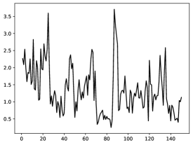
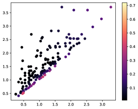
where has density and depends implicitly on and . For most of the Subsection 5.1, we perform our analysis on the realization displayed in Figure 2(a) of the trawl process with autocorrelation function and with simulation parameters and . The next step is to choose a value for which is representative of the values encountered in the iterations of the composite likelihood optimization procedure. We consider the pairwise densities at lag and their gradients for , where is estimated by GMM from . The two main reasons for studying the gradient estimators at are as follows. Firstly, the composite likelihood procedure requires a starting point, which we take to be in our experiments. Secondly, when is large, which ensures that is in the parameter region of interest and further motivates our choice. Next, we show in a simulation study that the PG methodology provides lower variance estimators than the SF one for the gradient of the pairwise densities. Afterwards, we perform a similar simulation study for the control variate methodology.
5.1.1 Pathwise gradients simulation results
Let and for . From (24), we see that for trawl processes with Gamma marginal distribution, the PG and SF methodologies give the following expressions for the gradient
for . Considering only the first term in the above equations allows us to isolate the part of the gradient which accounts for the dependency of the sampling measure on . Note that and do not depend on and we report just the partial derivatives with respect to and of the first term in the expression for the pairwise density. Let us settle the notation. With , define
Further define the gradients , the gradient estimators and , their standard deviations and and ratio of standard deviations
| (25) |
where the expectation is taken over with density and where we make the dependency of on the pairs is explicit.
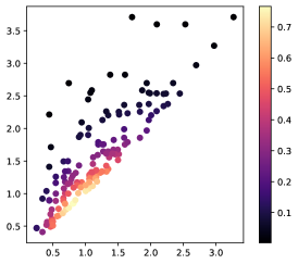
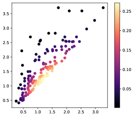
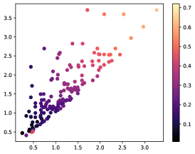
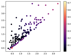
In the following, we display the values for the gradients of the pairwise densities, as well as the standard deviations of the corresponding MC estimators. We represent the pair as the pair and the corresponding quantity of interest through a color scheme, with a linear or log-scale color bar. Since the trawl process is stationary, we have that and for any value of . Thus sorting the pairs allows for an easier visual representation in the upper-triangular corner of the figures while making no theoretical difference in the gradient analysis. Figures 2(b) and 2(c) display the values of the partial derivatives and for . Figures 2(d) and 2(g) show the standard deviations of the SF estimators and for Note that the standard deviation of the SF estimators can even be two orders of magnitude higher than the corresponding values of the gradients, making accurate gradient calculations computationally expensive. Figures 2(e) and 2(h) show the ratios of the standard deviations of the PG and SF estimators and , as defined in (25); a value below favors the PG estimator over the SF one. Notice that the PG estimator always performs better and that it has a standard deviation which is reduced by a factor between and as compared to the standard deviation of the SF estimator; this improvement comes without an increase in the computation time. Finally, we show in Figures 2(f) and 2(i) that this improvement is maintained across a wide range of parameter regimes. To this end, we draw random samples from the priors . For each replication, we simulate a realisation of the trawl process with parameters and . From each , we compute the ratios of the standard deviations of the gradient estimators and ; we summarize the distributions of the two ratios above by computing the empirical and quantiles.
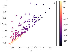
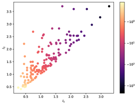
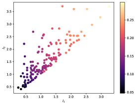


We then display the variability of these empirical quantiles across the simulations with boxplots in Figures 2(f) and 2(i) respectively. This allows us to study the variability in the distribution of the ratio of the standard deviations. For example, Figure 2(f) shows that in the vast majority of the simulations, the median of the ratio of standard deviations is about , as displayed in the boxplot for the quantile. This gives a variance reduction by a factor of . We also note that the PG estimator increases the variance of the estimator only in very few simulations, as can be seen from the boxplot outliers. We conclude that PG is an effective variance reduction method.
5.1.2 Control variate simulation results
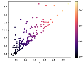
We show empirically that the control variates methodology can be employed to significantly reduce the variance of the estimators for both the pairwise densities and their gradients and that only a Taylor polynomial of a low degree is required. This also leads to a large reduction in the bias of the estimators for the log pairwise likelihood and its gradient . We display the quantities of interest via a color bar, as in Figure 2, first using the trawl path from Figure 2(a) for Figures 3(a)-3(f) and then with a simulation study in Figure 3(g). We define the standard deviation of the pairwise density estimators , the standard deviation of the same estimator with a Taylor polynomial of degree as control variate and the corresponding standard deviation ratio as follows
| (26) | ||||
where is from Example 3.1 and where we make explicit the dependency of the optimal constant on . The definition from (26) is ambiguous without specifying how is estimated. When employing this notation, we use the same samples to estimate the pairwise densities and the optimal constant and we specify how many samples we use.
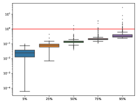
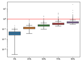
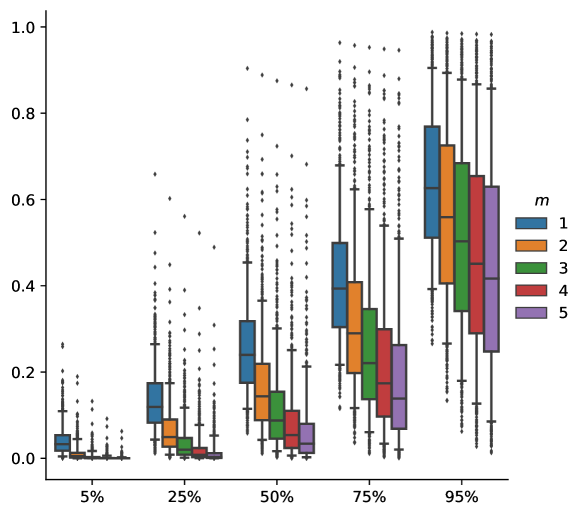
Figures 3(a) and 3(b) show the pairwise densities and the standard deviations of the corresponding estimators for , where is the GMM estimator. Figure 3(c) shows kernel density estimates of the estimators for with no control variate, i.e. , and with Taylor polynomials of degrees applied as control variates to each pair . To produce the plot, we use independent samples for each pair, from which we estimate both the pairwise density and . The kernel density estimate is based on replications, in each of which we use independent samples from , for each pair. The true value of , as estimated from samples with , is displayed through a vertical line. We note substantial bias and standard deviation reductions as we increase , even when we only use samples to calibrate . This further shows that in our setting, the performance of control variates is not sensitive to the miscalibration of the optimal constants. Finally, we show that the improvements are significant for a wide range of parameter regimes. We proceed as for Figures 2(f) and 2(i). To this end, we draw random samples from the prior . For each replication, we simulate a realisation of the trawl process processes with parameters and . From each we compute the empirical and quantiles of ; we then display the variability of these empirical quantiles across the simulations with a boxplot in Figure 3(g). We notice excellent variance reduction properties. In particular, even for , for over of the simulated paths, the median of the standard deviation ratio, i.e. the median of is below . For , in over of the simulated paths, the median of the standard deviation ratio drops below , reducing the number of samples required to achieve the same performance as the estimator by a factor of . We note that higher gives a higher variance reduction.
We turn our attention to the combined variance reduction properties of control variates and pathwise gradients for the estimation of the gradients and show that the improvements over the SF methodology are maintained even for long-memory trawl processes. To this end, let be a trawl process with and autocorrelation function , for , where and . Let be a realisation of the trawl process described above for and simulation parameters . Consider lags , let be the GMM estimators for and further
To obtain an estimator for , we use samples for each pair , where and ; we use the same samples to estimate both and . We repeat this computation times while keeping fixed to estimate the bias and variance of our SF and PG gradient estimators with Taylor polynomials of degree as control variates and show the results in Table 1. Note again that does not depend on , hence the SF and PG results are the same for this variable. We first analyze the case , which corresponds to not using control variates; as discussed in Subsection 4.2, the moments of are not always available in closed form. We see that the PG significantly outperforms SF for all parameters; for and , the bias and standard deviation are reduced by more than , respectively times. With control variates, the higher the , the better the bias and standard deviation properties and we see the same pattern as for . The PG methodology improves significantly over the SF one for and ; regarding the gradients with respect to for , PG has a slightly higher bias, although the standard deviation is significantly smaller than for the SF. We conclude that PG together with or removes the bias and decreases the variance enough to carry a gradient descent optimization procedure. We provide further tables with more evaluation metrics, e.g. mean absolute error (MAE), root-mean-square error (rMSE) and median absolute error (medAE) in Table 3 of Subsection S.3. For example, we see that the PG estimator has a much smaller MAE than the SF one. Thus the lower bias of SF for the partial derivative with respect to comes from larger errors that cancel out, as opposed to smaller errors that do not cancel for PG.
Remark 5.1.
In Table 1 we display the results only for one chosen value and do not provide simulation studies as in Figures 2(f), 2(i) and 3(g). The SF estimator becomes numerically unstable and returns infinite or non-numeric values when at least one of the parameters of is close to , where is the lag used and is the spacing between trawl sets. This issue often occurs for small or for small or large , i.e. when the autocorrelation or . Thus comparing the two methods in a simulation study is difficult, although it is worth noting that the PG is stable for a wide range of parameter regimes.
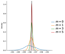
bias st. dev. bias st. dev. bias st. dev. bias st. dev. SF 4.19 5.25 0.27 1.92 0.07 1.43 0.00 1.20 -3.59 3.16 -0.58 1.80 -0.20 1.44 -0.04 1.15 7.88 9.11 0.61 2.11 0.22 1.44 0.10 1.14 -5.07 5.33 -0.39 1.44 -0.14 1.02 -0.06 0.81 PG 3.03 2.79 0.44 1.43 0.15 1.14 0.03 0.94 -3.59 3.16 -0.58 1.80 -0.20 1.44 -0.04 1.15 0.70 1.25 0.02 1.18 0.00 0.84 -0.03 0.67 -0.39 0.75 0.00 0.82 0.00 0.63 0.01 0.50
Practical considerations in the implementation of control variates
Our application of the control variates methodology to composite likelihood inference for trawl processes differs from the approach typically found in the modern stochastic optimization literature. Rather than utilizing reverse-mode automatic differentiation (AD) to compute the first-order derivatives of a mapping from high to low dimensional space, as commonly done in machine learning and deep learning, we require efficient computation of higher-order derivatives of a mapping from low to high dimensional, which can only be done using forward-mode AD. In spite of these computational challenges, we demonstrate that efficient implementations are possible and that our methodology is feasible. Additionally, we provide an overview of techniques that can be employed to accelerate the current numerical implementation. As before, let be the discretely observed path of the trawl process at times , the parameters which specify the distribution and autocorrelation structure of , the degree of the Taylor polynomial used as control variate and the lags used in the PL estimator. Then there are pairwise densities to approximate. Assume we use sets of i.i.d. samples to estimate each of the pairwise densities. Finally, let be the functions used to estimate each of the pairwise densities.
Firstly, the estimation of the optimal constants and turns out to involve the differentiation of a mapping from low to high dimensional space. For example, to estimate
we need to compute the gradient with respect to of the following two mappings
where . In this case, forward-mode and reverse-mode AD have computational complexity and , respectively. In general, is orders of magnitude lower than ; in our experiments, forward-mode AD works well, whereas reverse-mode AD fails due to the high complexity of the algorithm. The speed-up boils down to parenthesizing the Jacobian multiplications in the order which requires matrix-vector rather than matrix-matrix multiplications, as in the adjoint methods in design (see Chapter 8.7 of Strang (2007)). This step can be accelerated even further. Indeed, the optimal constants can be accurately estimated with a fraction of the samples used in the PL procedure; moreover, the optimal constants can be reused in consecutive iterations of gradient descent for an even lower computational cost.
Secondly, the control variates methodology heavily relies on the efficient computation of the higher order partial derivatives , for . Although atypical for modern frameworks such as Tensorflow and Torch, this has been studied extensively in previous works (Karczmarczuk, 1998; Pearlmutter & Siskind, 2008). In general, there is no formula for the complexity of calculating the first derivatives of in terms of the complexity of calculating , as this depends explicitly on the exact operations which put together define . It is thus difficult to define an effective sample size for the control variate methodology when taking into account the extra computational time. Although the simulation studies from Figure 3 and Table 1 display significant improvements with only a negligible increase in computational time for , using proved computationally expensive and the simulation study from Subsection 5.2 was carried out with . We argue or are generally good hyperparameter choices, as they already provide low-variance estimators which are essentially unbiased.
Remark 5.2.
It is not clear if the difficulty we face for large is due to theoretical reasons or sub-optimal implementations. For example, when applying the chain rule to compute the derivative of a composition of functions , one can group terms according to Faà di Bruno’s formula to avoid recomputing terms, similarly to the product rule for higher order derivatives. Our implementation in JAX does recompute terms, although new approaches to implement Faà di Bruno’s formula in JAX are now available (Bettencourt et al., 2019). We suspect this makes up most of the computational time. A task for further research is to see if removing the inefficiencies described above does indeed significantly lower the computational time, which in turn would allow to use little to no MC samples and approximate the pairwise densities by high-degree Taylor polynomials when the moments of are available analytically.
5.2 Parameter inference results
We demonstrate in a simulation study that the PL estimator achieves a lower estimation error than the GMM estimator outside of the Gaussian case. We note that in the Gaussian case, the two estimators are almost identical. To this end, we conduct a simulation study and consider the trawl processes with and multiple trawl functions. We set for Figures 4(a)-4(f) and for Figures 4(g)-4(i) and use the following parametric forms for the trawl function
For 4(a)-4(c) we infer , for 4(d)-4(f) we infer and for 4(g)-4(i) we infer . We compute the PL and GMM estimators from the discretely observed paths of the trawl processes described above, where . It remains to compare the two estimators. We remind the reader that the distributional properties of the trawl process are fully determined by its marginal distribution and autocorrelation function, which we can compare to assess the relative performance of the two estimators. For the marginal distribution, we compare the root-mean-square estimation error (rMSE) of and , as well as the mean Kullback–Leibler divergence (KL) between the marginal distributions of the trawl process, as inferred by PL and GMM. For the autocorrelation structure, comparing the estimation error of each parameter is only meaningful for trawl functions with a single parameter, e.g. in 4(a)-4(c) and in Figures 4(d)-4(f). For the two-parameter trawl function from Figures 4(g)-4(i), we can have very different values of giving similar shapes for the autocorrelation functions and comparing the per parameter estimation error is not meaningful. Instead, if and are the infered autocorrelation functions, we compare the weighted distance given by
where we set . We require a weighting function as and are not necessarily square-integrable, but note that the results are robust to varying . We display the ratio of these quantities (rMSE, mean KL divergence and mean weighted distance) in Figure 4; a ratio below favors the PL estimator and a ratio above favors the GMM estimator. Apart from Figure 4(g), where the autocorrelation (acf) and KL ratios show opposite trends, the PL significantly outperforms the GMM estimator. Similar results are displayed for the mean absolute error (MAE) and median absolute error (MedAE) in Figures 6 and 7 and in Tables 4a-4i in the Supplementary material. To understand the results better, we delve into the details of the numerical optimization routine.
Practical considerations in the optimization procedure
We carried out both the GMM and PL estimation procedures with the BFGS implementation from Python’s Scipy library, which requires starting points. For the GMM procedure, and were initialized at the method of the moments estimator, using the first two moments; , and were initialized at and finally, the PL procedure was initialized at the GMM estimator. For the long memory regime displayed in Figures 4(d)-4(i), the GMM procedure often diverged for , i.e. when the discretely observed path of the trawl process was too short; thus we display results starting at in these figures. Besides long memory, the optimization landscape is more complicated for trawl functions with more than one parameter, e.g. Figures 4(g)-4(i), where multiple local maxima exist. We found that in some of these simulations, e.g. when the GMM estimator is far away from the true value, the PL routine does not move much from the starting point. A task for further research is to see if running the optimization with multiple starting points or using a gradient descent procedure specifically designed for stochastically estimated gradients improves the result.
Both procedures need a set of lags . We found that both the PL and GMM procedures are robust in the sense that the choice of the hyperparameter does not influence the results considerably.
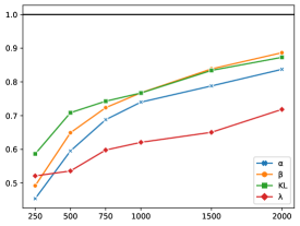
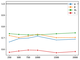
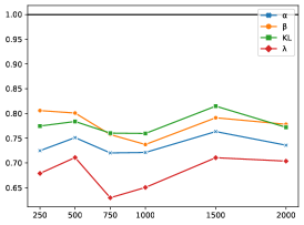
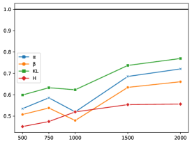
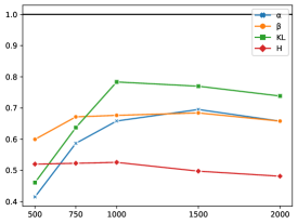
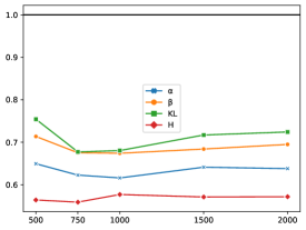
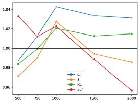
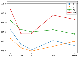
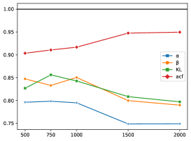
For Figure 4, we used in 4(d) and 4(g), in 4(a) and 4(e), in 4(a) and 4(f), in 4(h), in 4(i) and in 4(c).
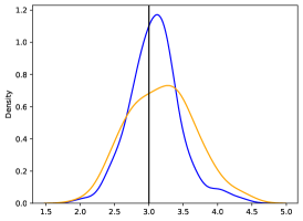
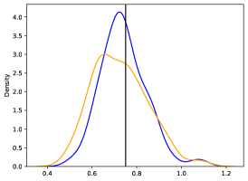
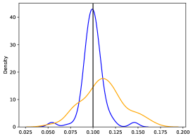
Finally, in Figure 5 we display kernel density estimates of the parameters and inferred with the PL and GMM methodologies for the simulation study from Figure 4(a) and . Similar patterns in which the PL performs better can be observed for a wide range of simulation parameters.
6 Applications to the forecasting of trawl processes
Let be the -algebra generated by the trawl process up to time and . In general, is not Markovian and is intractable, but we nevertheless approximate the distribution of by that of . Based on this idea, we introduce the first methodology for deterministic and probabilistic forecasting of real-valued trawl processes. For deterministic forecasting, we derive a novel conditional mean formula, which is optimal in the rMSE sense; we show that when used for forecasting, the parameters inferred by the PL methodology incur a smaller forecasting error than the ones inferred by the GMM methodology. For probabilistic forecasting, we discuss several methods to sample from the conditional distribution of . These samples can be also used for other types of deterministic forecasting, such as conditional median forecast, which is optimal in the sense of Mean Absolute Error (MAE). Finally, we discuss the integer-valued case at the end of the section.
We start with the conditional mean formula for deterministic forecasting.
Theorem 6.1.
Assume that the Lévy seed is integrable. Then
The above expression is a weighted average of the last observed value and of the mean, with . We carry out a simulation study in the setting of the Gamma trawl process with exponential trawl function from Figure 4(a). We use the PL and GMM methodologies to infer the parameter and from discretely observed paths of the trawl process of length . We further estimate and and then use the forecasting formula from Theorem 6.1. We approximate the PL and GMM out-of-sample forecasting errors (rMSE, MAE and MedAE) from simulated paths of the trawl process, each of length . We display in Table 2 the percentage change, i.e. , as a function of . We stress that the forecasting error is approximated on newly simulated paths of the trawl process, hence it is an out-of-sample error. We note that regardless of the lag at which we forecast, PL performs better than GMM, and that the improvement is bigger at smaller lags.
MAE MedAE rMSE MAE MedAE rMSE MAE MedAE rMSE MAE MedAE rMSE 1 -4.38 -13.48 -0.95 -1.44 -5.26 -0.19 -1.21 -4.46 -0.15 -0.47 -2.08 -0.04 2 -3.80 -9.13 -1.51 -1.19 -3.43 -0.34 -1.00 -2.77 -0.26 -0.37 -1.15 -0.06 3 -3.49 -7.39 -1.83 -1.09 -2.77 -0.45 -0.91 -2.29 -0.36 -0.32 -1.01 -0.09 4 -3.23 -6.32 -1.98 -1.01 -2.40 -0.53 -0.82 -1.97 -0.42 -0.29 -0.86 -0.10 5 -2.95 -5.39 -2.02 -0.94 -2.10 -0.58 -0.77 -1.77 -0.46 -0.26 -0.57 -0.11 6 -2.68 -4.79 -1.98 -0.88 -1.84 -0.61 -0.70 -1.54 -0.49 -0.24 -0.52 -0.12 8 -2.30 -3.75 -1.81 -0.77 -1.33 -0.62 -0.61 -0.93 -0.49 -0.21 -0.49 -0.12 10 -1.93 -3.02 -1.56 -0.65 -1.06 -0.56 -0.51 -0.75 -0.44 -0.18 -0.34 -0.10 12 -1.63 -2.44 -1.32 -0.54 -0.92 -0.49 -0.40 -0.78 -0.37 -0.13 -0.44 -0.08 15 -1.20 -1.80 -1.01 -0.39 -0.68 -0.38 -0.29 -0.48 -0.28 -0.08 -0.18 -0.05
For probabilistic forecasting, note that and that is independent of . The distribution of is given by the convolution of the distributions of and and, to sample from , it is enough to sample from and from . Assume we have a sampler for , which is the case for all the examples considered in this paper. If is Gaussian or Gamma distributed, then is Gaussian, respectively Beta distributed. In general, the conditional distribution of does not belong to named families, and we discuss two exact sampling techniques which generate independent samples. Note that the conditional density can be computed explicitly, as a product of known densities and a known normalizing constant.
Marrelec & Benali (2004) provides an exact sampling algorithm for the case where the density which requires sampling is proportional to a product of densities for which exact sampling methods are available. The authors perform rejection sampling and automate the choice of both the envelope function and upper bound constant. The algorithm is efficient even when dealing with a product of two heavy-tailed distributions, such as Cauchy, and does not require any extra information on the densities. The algorithm is inefficient and gives small acceptance rates when the two densities are peaked around two different values, e.g. and . In this case, we require further information on the densities. If for example we have a concave or log-concave density, we can perform efficient rejection sampling with a piecewise-linear, respectively piecewise-exponential envelope (Görür & Teh, 2012). The method can also be applied if we have access to the decomposition of the density or of its logarithm into convex and concave components. The above sampling techniques can further be combined with MCMC methods, such as in Adaptive Rejection Metropolis-Hastings, although these extensions only produce dependent, asymptotic samples from the target density.
For Integer-valued trawl processes (IVT), the conditional mean forecast from Theorem 6.1 is not integer-valued, hence it is not data-coherent. Instead, the conditional median or mode can be used, and, the conditional distributions are often part of named distributions (see Section 4 of Bennedsen et al. (2023)). Even when this is not the case, the conditional probabilities are given by finite or countable sums, which can be calculated exactly or approximated by truncation. In both the real-valued and integer-valued cases and for both deterministic and probabilistic forecasting, the forecasting error only shows minimal improvements in spite of the significantly improved parameter fit. One potential explanation is the simplicity of our forecasting formula, which only allows conditioning on the last lag. A task for further research is to derive a forecasting formula conditional on more lags and investigate the associated forecasting error. We expect that with more lags involved, the improved PL parameter fit, together with the non-Markovianity of trawl processes will result in further improvements in the forecasting error.
7 Conclusion
This paper develops the first likelihood-based methodology for the inference of continuous-time, real-valued trawl processes and introduces a novel deterministic forecasting formula for these processes. The contributions are threefold.
Firstly, we reduce the variance of the estimators for the pairwise likelihood (PL) and its gradients by several orders of magnitude and show that PL inference for trawl processes is accurate and computationally efficient. We provide Python implementations at Leonte (2023) which integrate our methodology with automatic differentiation engines, eliminating the need for manual calculations and enabling easy adaptation to fit trawl processes with other marginal distributions and trawl functions.
Secondly, we demonstrate the excellent finite sample properties of the PL estimator in a simulation study, showing a large reduction in estimation error compared to the generalized method of moments (GMM) estimator. The PL estimator consistently and significantly outperforms the GMM estimator, regardless of the number of lags used, length of the discretely observed path of the trawl process, or metric employed to evaluate the parameter fit: mean squared or absolute error, median absolute error or KL divergence.
Thirdly, we derive a novel conditional mean forecasting formula and present the first methodology for the probabilistic forecasting of continuous-time, real-valued trawl processes. In a simulation study, we demonstrate that the PL estimator outperforms the GMM estimator in out-of-sample forecasting errors.
Finally, our work begins to bridge the gap between theoretical studies of trawl processes and ambit fields and the use of deep learning techniques to fit the model parameters. We hope that this article will contribute towards both the methodological development of the field of Ambit Stochastics and its integration into routine statistical modelling toolkits.
Acknowledgements
We would like to thank Dan Crisan and Tony Wang for constructive discussions and comments on earlier versions of the manuscript. Dan Leonte acknowledges support from the EPSRC Centre for Doctoral Training in Mathematics of Random Systems: Analysis, Modelling and Simulation (EP/S023925/1).
References
- (1)
-
Barndorff-Nielsen (2011)
Barndorff-Nielsen, O. E. (2011), ‘Stationary
infinitely divisible processes’, Brazilian Journal of Probability and
Statistics 25(3), 294 – 322.
https://doi.org/10.1214/11-BJPS140 -
Barndorff-Nielsen et al. (2018)
Barndorff-Nielsen, O. E., Benth, F. E. & Veraart, A. E.
(2018), Ambit Stochastics,
Springer-Verlag, Berlin.
https://doi.org/10.1007/978-3-319-94129-5 -
Barndorff-Nielsen et al. (2014)
Barndorff-Nielsen, O. E., Lunde, A., Shephard, N. & Veraart, A. E.
(2014), ‘Integer-valued trawl processes: A
class of stationary infinitely divisible processes’, Scandinavian
Journal of Statistics 41(3), 693–724.
https://doi.org/10.1111/sjos.12056 -
Bennedsen et al. (2023)
Bennedsen, M., Lunde, A., Shephard, N. & Veraart, A. E.
(2023), ‘Inference and forecasting for
continuous-time integer-valued trawl processes’, Journal of
Econometrics 236(2), 105476.
https://doi.org/10.1016/j.jeconom.2023.105476 -
Bettencourt et al. (2019)
Bettencourt, J., Johnson, M. J. & Duvenaud, D. (2019), Taylor-mode automatic differentiation for
higher-order derivatives in Jax, in ‘Program Transformations for ML
Workshop at NeurIPS 2019’.
https://openreview.net/forum?id=SkxEF3FNPH - Bradley & Taqqu (2003) Bradley, B. O. & Taqqu, M. S. (2003), Financial risk and heavy tails, in ‘Handbook of heavy tailed distributions in finance’, Elsevier, pp. 35–103.
- Caers et al. (1999) Caers, J., Beirlant, J. & Maes, M. A. (1999), ‘Statistics for modeling heavy tailed distributions in geology: Part i. methodology’, Mathematical Geology 31, 391–410.
-
Cui et al. (2022)
Cui, Z., Liu, Y. & Wang, R. (2022), ‘Variance comparison between infinitesimal perturbation analysis and
likelihood ratio estimators to stochastic gradient’, Operations Research
Letters 50(2), 199–204.
https://doi.org/10.1016/j.orl.2022.01.012 - Fan et al. (2015) Fan, K., Wang, Z., Beck, J., Kwok, J. & Heller, K. A. (2015), ‘Fast second order stochastic backpropagation for variational inference’, Advances in Neural Information Processing Systems 28.
-
Figurnov et al. (2018)
Figurnov, M., Mohamed, S. & Mnih, A. (2018), Implicit reparameterization gradients, in
S. Bengio, H. Wallach, H. Larochelle, K. Grauman, N. Cesa-Bianchi
& R. Garnett, eds, ‘Advances in Neural Information Processing
Systems’, Vol. 31, Curran Associates, Inc.
https://proceedings.neurips.cc/paper/2018/file/92c8c96e4c37100777c7190b76d28233-Paper.pdf - Fu (2006) Fu, M. C. (2006), Chapter 19 gradient estimation, in S. G. Henderson & B. L. Nelson, eds, ‘Simulation’, Vol. 13 of Handbooks in Operations Research and Management Science, Elsevier, pp. 575–616.
- Gal (2016) Gal, Y. (2016), Uncertainty in Deep Learning, PhD thesis, University of Cambridge.
- Glasserman (2004) Glasserman, P. (2004), Monte Carlo methods in financial engineering, Vol. 53 of Applications of Mathematics (New York), Springer-Verlag, New York. Stochastic Modelling and Applied Probability.
-
Görür & Teh (2012)
Görür, D. & Teh, Y. (2012),
‘Concave-convex adaptive rejection sampling’, Journal of Computational
and Graphical Statistics 20, 670–691.
https://doi.org/10.1198/jcgs.2011.09058 -
Ho & Cao (1983)
Ho, Y. & Cao, X. (1983),
‘Perturbation analysis and optimization of queueing networks’, Journal
of Optimization Theory and Applications 40(4), 559–582.
https://doi.org/10.1007/BF00933971 -
Jankowiak & Obermeyer (2018)
Jankowiak, M. & Obermeyer, F. (2018), Pathwise derivatives beyond the reparameterization
trick, in J. G. Dy & A. Krause, eds, ‘Proceedings of the
35th International Conference on Machine Learning, ICML 2018,
Stockholmsmässan, Stockholm, Sweden, July 10-15, 2018’, Vol. 80 of Proceedings of Machine Learning Research, PMLR, pp. 2240–2249.
http://proceedings.mlr.press/v80/jankowiak18a.html -
Jónsdóttir et al. (2013)
Jónsdóttir, K. Y., Rønn-Nielsen, A., Mouridsen, K. & Vedel Jensen, E. B. (2013), ‘Lévy-based
modelling in brain imaging’, Scandinavian Journal of Statistics 40(3), 511–529.
https://doi.org/10.1002/sjos.12000 -
Karczmarczuk (1998)
Karczmarczuk, J. (1998), ‘Functional
differentiation of computer programs’, SIGPLAN Not. 34(1), 195–203.
https://doi.org/10.1145/291251.289442 - Kingma & Welling (2013) Kingma, D. P. & Welling, M. (2013), ‘Auto-encoding variational bayes’, arXiv preprint arXiv:1312.6114 .
- Kleijnen & Rubinstein (1996) Kleijnen, J. P. & Rubinstein, R. Y. (1996), ‘Optimization and sensitivity analysis of computer simulation models by the score function method’, European Journal of Operational Research 88(3), 413–427.
- Knowles (2015) Knowles, D. A. (2015), ‘Stochastic gradient variational bayes for gamma approximating distributions’, arXiv: Machine Learning .
-
Leonte (2023)
Leonte, D. (2023), ‘Ambit stochastics’,
https://github.com/danleonte/Ambit_Stochastics.
GitHub repository.
https://doi.org/10.5281/zenodo.7081978 -
Leonte & Veraart (2023)
Leonte, D. & Veraart, A. E. (2023), ‘Simulation methods and error analysis for trawl processes and ambit
fields’, Mathematics and Computers in Simulation .
https://doi.org/10.1016/j.matcom.2023.07.018 -
Marrelec & Benali (2004)
Marrelec, G. & Benali, H. (2004),
‘Automated rejection sampling from product of distributions’, Comput.
Statist. 19(2), 301–315.
https://doi.org/10.1007/BF02892062 -
Mátyás (1999)
Mátyás, L., ed. (1999), Generalized Method of Moments Estimation, Vol. 5 of Themes in Modern
Econometrics, Cambridge University Press.
https://doi.org/10.1017/CBO9780511625848 - Mikhailov (1967) Mikhailov, G. A. (1967), ‘Calculation of derivatives of the functionals of the transport equation solution over system parameters by monte carlo method’, Zh.Vychisl.Mat.Mat.Fiz. 7(4), 915–919.
- Miller (1967) Miller, L. B. (1967), Monte carlo analysis of reactivity coefficients in fast reactors general theory and applications, Technical report, Argonne National Lab.(ANL), Argonne, IL (United States).
-
Mohamed et al. (2020)
Mohamed, S., Rosca, M., Figurnov, M. & Mnih, A. (2020), ‘Monte Carlo gradient estimation in machine
learning’, J. Mach. Learn. Res. 21, Paper No. 132, 62.
http://jmlr.org/papers/v21/19-346.html - Naesseth et al. (2017) Naesseth, C., Ruiz, F., Linderman, S. & Blei, D. (2017), Reparameterization gradients through acceptance-rejection sampling algorithms, in ‘Artificial Intelligence and Statistics’, PMLR, pp. 489–498.
-
Nguyen & Veraart (2017)
Nguyen, M. & Veraart, A. E. D. (2017), ‘Spatio-temporal Ornstein–Uhlenbeck processes:
Theory, simulation and statistical inference’, Scandinavian Journal of
Statistics 44(1), 46–80.
https://doi.org/10.1111/sjos.12241 - Nørvang Andersen & Asmussen (2011) Nørvang Andersen, L. & Asmussen, S. (2011), ‘Local time asymptotics for centered lévy processes with two-sided reflection’, Stochastic models 27(2), 202–219.
-
Noven (2016)
Noven, R. C. (2016), Statistical Models for
Spatio-Temporal Extrema and Dependencies, PhD thesis, Imperial College
London.
https://doi.org/10.25560/48048 - Pearlmutter & Siskind (2008) Pearlmutter, B. A. & Siskind, J. M. (2008), Using programming language theory to make automatic differentiation sound and efficient, in C. H. Bischof, H. M. Bücker, P. Hovland, U. Naumann & J. Utke, eds, ‘Advances in Automatic Differentiation’, Springer Berlin Heidelberg, Berlin, Heidelberg, pp. 79–90.
- Pflug (1996) Pflug, G. C. (1996), Optimization of stochastic models: the interface between simulation and optimization, Kluwer Academic Publishers.
-
Podgórski & Wallin (2016)
Podgórski, K. & Wallin, J. (2016), ‘Convolution-invariant subclasses of generalized hyperbolic distributions’,
Communications in Statistics - Theory and Methods 45(1), 98–103.
https://doi.org/10.1080/03610926.2013.821489 -
Rezende et al. (2014)
Rezende, D. J., Mohamed, S. & Wierstra, D. (2014), Stochastic backpropagation and approximate inference
in deep generative models, in ‘International conference on machine
learning’, PMLR, pp. 1278–1286.
https://proceedings.mlr.press/v32/rezende14.html - Robinson (2003) Robinson, P. M. (2003), Time series with long memory, Advanced Texts in Econometrics.
- Rubinstein (1969) Rubinstein, R. Y. (1969), Some problems in Monte Carlo optimization, PhD thesis, University of Riga, Latvia.
-
Rubinstein (1992)
Rubinstein, R. Y. (1992), ‘Sensitivity
analysis of discrete event systems by the “push out” method’, Annals
of Operations Research 39(1), 229–250.
https://doi.org/10.1007/BF02060943 - Ruiz et al. (2016) Ruiz, F., Titsias, M. & Blei, D. (2016), ‘The generalized reparameterization gradient’, Advances in Neural Information Processing Systems 0, 460–468.
- Sato (1999) Sato, K. (1999), Lévy processes and infinitely divisible distributions, Vol. 68 of Cambridge Studies in Advanced Mathematics, Cambridge University Press, Cambridge. Translated from the 1990 Japanese original, Revised by the author.
-
Sauri & Veraart (2022)
Sauri, O. & Veraart, A. E. D. (2022), ‘Nonparametric estimation of trawl processes: Theory
and applications’.
https://arxiv.org/abs/2209.05894 - Strang (2007) Strang, G. (2007), Computational science and engineering, Vol. 791, Wellesley-Cambridge Press Wellesley.
-
Vershynin (2018)
Vershynin, R. (2018), High-dimensional
probability, Vol. 47 of Cambridge Series in Statistical and
Probabilistic Mathematics, Cambridge University Press, Cambridge.
An introduction with applications in data science, With a foreword by
Sara van de Geer.
https://doi.org/10.1017/9781108231596 -
Williams (1992)
Williams, R. J. (1992), ‘Simple statistical
gradient-following algorithms for connectionist reinforcement learning’, Machine learning 8(3), 229–256.
https://doi.org/10.1007/BF00992696 -
Wolpert & Taqqu (2005)
Wolpert, R. & Taqqu, M. (2005),
‘Fractional Ornstein-Uhlenbeck Lévy processes and the Telecom
process: Upstairs and downstairs’, Signal Processing 85, 1523–1545.
https://doi.org/10.1016/j.sigpro.2004.09.016
Appendix
The appendix contains a list of the parameterizations of all the probability distributions used in this paper: Poisson, Negative binomial (NB), Skellam, Uniform, Beta, Gamma, inverse Gaussian (IG), Gaussian (), double-sided Maxwell (), Normal-inverse Gaussian (NIG), and Variance-gamma (VG).We denote by and by . Let and be the modified Bessel function of the first, respectively second kind.
| Discrete Distributions | |||||
|---|---|---|---|---|---|
| Distribution | Range | Parameters | PMF | ||
|
|
|||||
| Continuous Distributions | |||||
| Distribution | Range | Parameters | |||
|
|
|||||
|
|
|||||
|
|
|||||
Definition A.1 (Normal variance-mean mixture).
We say follows a normal variance-mean mixture distribution with mixing density if
where has pdf , and and are independent. Then . We discuss two particular cases.
If the constants are and the mixing density is given by , where , then . We obtain the the Normal-inverse Gaussian distribution, and .
Supplementary material
Likelihood-based inference and forecasting for trawl processes: a stochastic optimization approach
| Dan Leonte and Almut E. D. Veraart |
| Department of Mathematics, Imperial College London |
The supplementary material is structured as follows.
-
•
Section S.1 contains technical derivations and proofs. Subsection S.1.1 discusses the bias, variance and probabilistic bounds for the estimators of the pairwise density and its gradient. We derive expressions for the asymptotic bias and variance of these estimators and establish the corresponding convergence rates. Subsection S.1.2 gives the proof of the novel deterministic forecasting formula.
-
•
Section S.2 derives a novel chain rule for stochastic transformations and introduces hybrid estimators, which combine PG and MVG and greatly extends the applicability of our methodology; in particular, it allows for PL inference of integer-valued trawl processes.
- •
S.1 Proofs
In this section we present the proofs which were omitted from the main body of the paper.
S.1.1 Asymptotic bias, variance and probabilistic bounds
Fix and let for . We have seen in Subsection 3.3 that both the pairwise density and its gradient can be written as Monte Carlo (MC) estimators, i.e. and for some functions , and density parameterized by . The function is the product of marginal densities of the trawl process (see (20)), hence strictly positive; is given by in the SF estimator and by in the PG estimator. Finally, is either the density of for some set , if is real-valued, or the truncation of such a density to if is positive real-valued. We show next that the properties of determine the rate of convergence of the MC estimators.
Likelihood estimation and the Jensen gap
Let be a sequence of iid random variables with density . Then the random variables given by for are strictly positive, iid, unbiased and consistent estimators for . Let . By Jensen’s inequality, the estimator overestimates . To quantify the properties of this estimator, we derive its asymptotic bias and variance. By applying the Taylor expansion , we have that
By taking the expectation and variance of both sides and neglecting higher-order terms, we obtain that
hence the asymptotic bias and variance for are given by
This highlights the importance of having low variance estimators, not only to reduce the variability, but also the bias of . Further, the estimated value of can be used for an adaptive procedure, to calibrate the number of required samples for each pair . We can also provide non-asymptotic, probabilistic bounds. By the mean value theorem, we have that for some random variable in between and a.s. Further
For , we have that implies that , hence
and
where . The rate of decay in the above inequality depends on the distribution of , where is distributed according to . If for example is compactly supported, as in Example 3.1, then Lemma S.2 applies and the convergence of to is exponential in the number of samples , with an exponential rate depending on the pair . The exponential convergence also holds if is sub-Gaussian, as in the case of the Gaussian Lévy seed, or sub-exponential, as in the case of the IG and NIG Lévy seeds. The exponential rates of convergence depend again on and can be deduced from Lemma S.1. If has a heavy tailed distribution, as is the case for Cauchy Lévy seeds, the convergence is polynomial and not exponential. A detailed analysis of concentration inequalities can be found in Vershynin (2018).
Concentration inequalities
Lemma S.1 (Chernoff bounds).
Let be a real-valued random variable. Then
A similar bound can be obtained for by replacing with in the above inequality. We specialize the above to sub-Gaussian and sub-exponential distributions. In the following, are iid with mean and .
We say is sub-Gaussian if for any . If are iid, sub-Gaussian random variables with mean , then is sub-Gaussian and
Alternatively, we say is sub-Exponential if for . Then
If are compactly supported, we can further refine the above Chernoff bounds.
Lemma S.2 (Hoeffding’s inequality).
Let be iid random variables with mean such that a.s. for . Let . Then
Gradient estimation
As before, let be a sequence of iid random variables with density , and further . Although the sequences and have independent terms, and are dependent. By taking the Taylor expansion of
at and where , we obtain that
By taking the expectation and variance of both sides and neglecting higher-order terms, we obtain that
| (27) | ||||
| (28) |
where to obtain (27) and (28), we expand the variance and covariance terms and use that and are independent when . Note that Jensen’s inequality does not apply to the map , as and are dependant, and the ratio estimator can have both positive and negative asymptotic bias. The asymptotic bias and variance of are then given by
respectively. Non-asymptotic bounds on the deviation of the gradient estimators from the gradient of the log-likelihood can be produced individually for each family of distributions , by analyzing the asymptotic growth or decay of as .
S.1.2 Forecasting formula proof
We now prove Theorem 6.1, for which we need the following two results.
Lemma S.3.
Let be integrable and exchangeable real-valued random variables. Then
Lemma S.4.
Let be a sequence of weakly convergent infinitely divisible random variables, with Lévy-Khintchine triplets . Then for :
Lemma S.3 is well known; the proof for Lemma S.4 can be found in Nørvang Andersen & Asmussen (2011).
Proof of Theorem 6.1.
By the independence of and , we have that
hence it is enough to prove that
| (29) |
We prove (29) by analysing two cases.
Case I: If for some positive integers and , let
and partition into disjoint subsets of area and into disjoint subsets of area Then are iid and integrable and by Lemma S.3, we obtain that
Case II: If let with Consider a nested sequences of sets such that
By the proof of Case I, we have that . Since we have that a.s. By the uniqueness of the limit, it is enough to prove that in , or equivalently in . We show that the sequence convergence in probability to and is uniformly integrable. We have that
Thus in distribution and in probability. It remains to prove the uniform integrability property. Let be the Lévy-Khintchine triplet of the Lévy seed Then the Lévy-Khintchine triplets of are given by , where as . We obtain that
Since is integrable, it follows that is finite (cf. Sato 1999, Theorem 25.3), hence by the dominated convergence theorem
By Lemma S.4, the sequence is uniformly integrable, which finishes the proof.∎
S.2 Measure-valued gradients and hybrid estimators
In the main part of the paper, we formulated composite likelihood inference for trawl processes as a stochastic optimization problem and expressed both the pairwise density and its gradient as Monte Carlo (MC) estimators, where depends implicitly on and . We found that the conventional finite difference and score function (SF) methods yield impractical estimators for the gradient of the log density, as they suffer from large biases and variances. However, we demonstrated the feasibility of composite likelihood inference by deriving lower variance estimators with the method of pathwise gradients (PG), which can be easily applied to a wide range of continuous distributions. To utilize the PG methodology, there are three requirements: the pathwise gradient must be available numerically for samples with density , the function must be differentiable in and the interchange between differentiation and integration must be valid. Under these conditions, the MC estimator for the gradient is then given by
We greatly extend the gradient estimation methodology by relaxing the first two requirements while retaining the last one. We start by explaining why such extensions are important. Firstly, PG are generally not available for discrete distributions (cf. Fu 2006, p. 595 - 597); secondly, even if is smooth, the partial derivative might be difficult to compute. Illustrating both issues is the Skellam Lévy basis from Example 2.7, for which the pairwise mass function is given by
where are the Lebesgue measures of the slices (see Figure 1 and (5)). The above can be estimated via Monte Carlo samples by taking the expectation over any of ; working with , we obtain that
where and is the modified Bessel function of the firs kind. Although is differentiable in both arguments, we are not aware of computer implementations for . Further, PG are not available for the Skellam distribution. Motivated by these two issues, we give an overview of MVG and explain how MVG can be used to obtain low-variance MC estimators for the gradient of the pairwise mass function for Integer-valued trawl (IVT) processes; we illustrate with the Poisson and Skellam Lévy bases. For the cases when MVG are not available (e.g. the Negative Binomial distribution), we derive hybrid estimators, which combine PG and MVG and provide a unified inference methodology, applicable to both integer-valued and real-valued trawl processes. In doing so, we formalize a chain rule for the class of stochastic transformations given by conditional sampling, which can be applied outside the trawl processes framework to derive low-variance gradient estimators in a wide range of stochastic optimization tasks, e.g. in deep learning.
Given a probability mass function parameterized by , the MVG method uses the decomposition of the signed measure induced by the unnormalized probability mass functions into , where are positive constants and are probability measures parameterized by for . In shorthand, we have
where are dimensional vectors with positive entries and are dimensional vectors of probability measure. We discuss the practical implementation details, non-uniqueness of the pair and variance reduction by coupling in the Poisson and Skellam cases.
Example S.5 (Poisson distribution).
Let with , where is the Dirac delta function at . Then the unnormalized probability mass function
can be decomposed in at least two ways. Firstly, we can set
where
and where and are the floor, respectively ceiling functions. This is the Hahn-Jordan decomposition of into measures with disjoint support. A simpler decomposition is given by
which are the probability mass functions of a Poisson distribution shifted by one unit, respectively of a Poisson distribution, and . The latter decomposition is much easier to implement on a computer. Using the latter decomposition, the MVG estimator is given by
| (30) |
where . The samples from can be generated by adding to the samples from , halving the simulation computational cost. Using dependent samples for and instead of independent ones generally reduces the variance of the resulting estimator, as observed in Example 4.12 of (Pflug 1996) and the simulation study from (Mohamed et al. 2020).
Example S.6 (Skellam distribution).
Note that , where are independent. Thus we can obtain MVG for the Skellam distribution from the MVG of the Poisson distribution.
Next, we discuss hybrid estimators for distributions for which neither PG nor MVG is directly available, generalizing Lemma 4.8. These estimators can be implemented in practice when samples from can be generated by sequential conditional sampling from distributions for which either PG or MVG are available. An illustrative example is the Negative Binomial (NB) distribution: if and then . To this end, we formalize the chain rule applied to the composition of stochastic transformations , where each of the sampling procedures and have either PG or MVG. In the following, is a density and can be either a density or a probability mass function.
Lemma S.7 (Chain rule for stochastic transformations).
Let be random variables with distributions where the conditional distribution of is given by and such that we can sample from and for any value of . Suppose that we can compute the PG of .
i) Suppose further that we can compute the PG of for any value of . Then
| (31) |
ii) Suppose further that an MVG decomposition of is available and that conditional on any value of , we can sample random variables distributed according to and . Then
| (32) |
Proof of Lemma S.7.
S.3 Extended simulation study for trawl processes
We present further simulation study results for the variance reduction properties of our gradient estimation methodology and for the improved finite sample performance of the PL estimator over the GMM estimator.
Variance reduction
In Table 1 of Subsection 5.1 we displayed the bias and standard deviation of the gradient estimators. In practice, we are more interested in the absolute deviations from the true value of the gradient, as displayed in Table 3, rather than the bias. We note that the PG estimator always has a smaller deviation from the true value, regardless of the metric: mean absolute error (MAE), median absolute error (MedAE) or root-mean-square error (rMSE).
MAE MedAE rMSE MAE MedAE rMSE MAE medAE rMSE MAE MedAE rMSE SF 5.44 4.72 7.56 1.51 1.23 2.44 1.13 0.92 1.83 0.95 0.78 1.53 4.02 3.82 5.11 1.51 1.28 2.35 1.16 0.99 1.85 0.91 0.77 1.47 9.89 8.67 13.44 1.72 1.40 2.72 1.15 0.95 1.84 0.91 0.74 1.46 6.07 5.27 8.08 1.17 0.99 1.86 0.81 0.67 1.30 0.64 0.52 1.04 PG 3.45 3.26 4.44 1.20 1.02 1.86 0.93 0.82 1.47 0.74 0.62 1.19 4.02 3.82 5.11 1.51 1.28 2.35 1.16 0.99 1.85 0.91 0.77 1.47 1.14 0.95 1.69 0.93 0.77 1.50 0.68 0.60 1.08 0.52 0.44 0.85 0.67 0.58 1.01 0.65 0.55 1.05 0.51 0.45 0.81 0.40 0.33 0.64
Parameter inference
In Figure 4 of Subsection 5.2 we showed that the PL estimator achieves a lower rMSE than the GMM estimator. We show in Figures 6 and 7 that the improvement is maintained if instead of rMSE we use MAE or MedAE. We also provide Tables 4a-4i with all the metrics from Figures 4, 6 and 7 together.
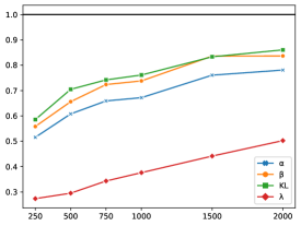
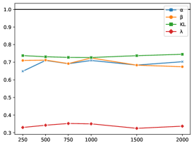
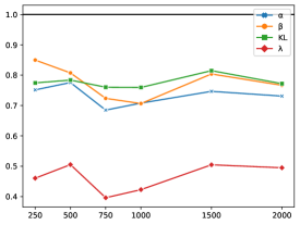
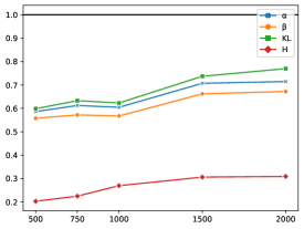
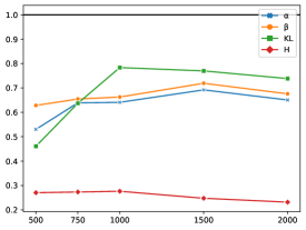
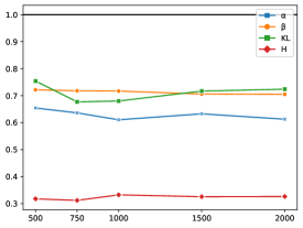
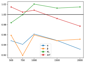
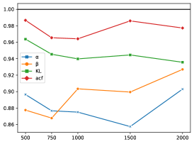
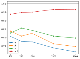
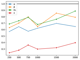
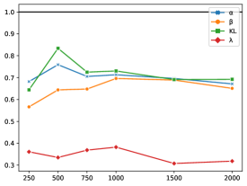
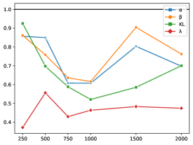
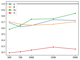
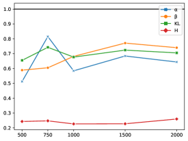
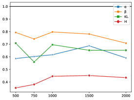
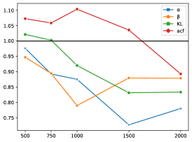
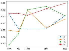
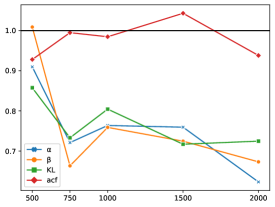
KL rMSE MAE MedAE rMSE MAE MedAE MKL MedKL rMSE MAE MedAE 2000 0.84 0.80 0.65 0.89 0.85 0.79 0.87 0.89 0.72 0.52 0.40 1500 0.79 0.76 0.70 0.84 0.84 0.86 0.83 0.76 0.65 0.42 0.32 1000 0.74 0.68 0.62 0.77 0.75 0.65 0.77 0.68 0.62 0.39 0.30 750 0.69 0.66 0.58 0.72 0.72 0.80 0.74 0.79 0.60 0.36 0.36 500 0.60 0.61 0.65 0.65 0.66 0.70 0.71 0.74 0.54 0.29 0.28 250 0.45 0.52 0.57 0.49 0.57 0.63 0.59 0.69 0.52 0.27 0.24
.
KL rMSE MAE MedAE rMSE MAE MedAE MKL MedKL rMSE MAE MedAE 2000 0.69 0.70 0.67 0.70 0.67 0.65 0.74 0.69 0.58 0.34 0.32 1500 0.68 0.68 0.70 0.70 0.68 0.69 0.74 0.69 0.57 0.32 0.31 1000 0.72 0.71 0.71 0.73 0.72 0.70 0.73 0.73 0.59 0.35 0.38 750 0.70 0.69 0.71 0.72 0.69 0.65 0.73 0.72 0.59 0.35 0.37 500 0.69 0.71 0.76 0.70 0.71 0.64 0.73 0.83 0.58 0.34 0.34 250 0.66 0.65 0.68 0.72 0.71 0.57 0.74 0.64 0.57 0.33 0.36
KL rMSE MAE MedAE rMSE MAE MedAE MKL MedKL rMSE MAE MedAE 2000 0.74 0.73 0.70 0.78 0.77 0.76 0.77 0.70 0.70 0.50 0.47 1500 0.76 0.75 0.80 0.79 0.80 0.90 0.81 0.59 0.71 0.50 0.48 1000 0.72 0.71 0.61 0.74 0.71 0.62 0.76 0.52 0.65 0.42 0.46 750 0.72 0.68 0.61 0.76 0.72 0.64 0.76 0.59 0.63 0.40 0.43 500 0.75 0.78 0.85 0.80 0.81 0.76 0.78 0.70 0.71 0.51 0.56 250 0.72 0.75 0.86 0.81 0.85 0.86 0.77 0.92 0.68 0.46 0.37
KL rMSE MAE MedAE rMSE MAE MedAE MKL MedKL rMSE MAE MedAE 2000 0.72 0.71 0.73 0.66 0.67 0.70 0.77 0.84 0.56 0.31 0.25 1500 0.69 0.71 0.74 0.63 0.66 0.66 0.74 0.75 0.55 0.31 0.29 1000 0.52 0.60 0.64 0.48 0.57 0.65 0.62 0.75 0.52 0.27 0.24 750 0.59 0.61 0.62 0.54 0.57 0.66 0.63 0.64 0.47 0.23 0.21 500 0.53 0.59 0.69 0.51 0.56 0.70 0.60 0.58 0.45 0.20 0.19
KL rMSE MAE MedAE rMSE MAE MedAE MKL MedKL rMSE MAE MedAE 2000 0.66 0.65 0.64 0.66 0.68 0.74 0.74 0.71 0.48 0.23 0.26 1500 0.70 0.69 0.68 0.68 0.72 0.77 0.77 0.72 0.50 0.25 0.23 1000 0.66 0.64 0.58 0.68 0.66 0.68 0.78 0.68 0.53 0.28 0.23 750 0.59 0.64 0.81 0.67 0.65 0.60 0.64 0.74 0.52 0.27 0.25 500 0.42 0.53 0.51 0.60 0.63 0.59 0.46 0.65 0.52 0.27 0.24
KL rMSE MAE MedAE rMSE MAE MedAE MKL MedKL rMSE MAE MedAE 2000 0.64 0.61 0.59 0.69 0.70 0.71 0.72 0.65 0.57 0.33 0.43 1500 0.64 0.63 0.69 0.68 0.71 0.78 0.72 0.65 0.57 0.33 0.45 1000 0.62 0.61 0.62 0.67 0.72 0.80 0.68 0.70 0.58 0.33 0.45 750 0.62 0.64 0.60 0.68 0.72 0.74 0.68 0.56 0.56 0.31 0.38 500 0.65 0.65 0.59 0.71 0.72 0.79 0.75 0.71 0.56 0.32 0.35
KL acf rMSE MAE MedAE rMSE MAE MedAE MKL MedKL rWMSE WMAE WMedAE 2000 1.03 0.93 0.78 0.99 0.95 0.88 1.01 0.83 0.98 0.96 0.89 1500 1.03 0.95 0.73 0.99 0.95 0.88 1.01 0.83 0.99 0.99 1.04 1000 1.04 0.96 0.88 1.03 0.96 0.79 1.02 0.92 1.01 1.02 1.10 750 1.01 0.94 0.89 0.99 0.92 0.89 1.00 1.00 1.00 1.01 1.06 500 0.99 0.95 0.98 0.97 0.96 0.95 0.98 1.02 1.01 1.03 1.07
KL acf rMSE MAE MedAE rMSE MAE MedAE MKL MedKL rWMSE WMAE WMedAE 2000 0.91 0.90 0.91 0.92 0.93 0.88 0.94 0.91 0.98 0.97 1.00 1500 0.92 0.86 0.81 0.91 0.90 0.82 0.94 0.98 0.99 0.98 0.96 1000 0.90 0.88 0.81 0.90 0.90 0.95 0.94 0.95 0.96 0.94 0.91 750 0.91 0.88 0.81 0.91 0.87 0.79 0.95 0.77 0.97 0.94 0.92 500 0.94 0.90 0.92 0.93 0.88 0.80 0.96 0.69 0.99 0.99 0.92
KL acf rMSE MAE MedAE rMSE MAE MedAE MKL MedKL rWMSE WMAE WMedAE 2000 0.75 0.72 0.62 0.79 0.75 0.67 0.80 0.72 0.97 0.95 0.94 1500 0.75 0.74 0.76 0.80 0.76 0.72 0.81 0.72 0.97 0.95 1.04 1000 0.79 0.77 0.76 0.85 0.83 0.76 0.84 0.80 0.95 0.92 0.98 750 0.80 0.78 0.72 0.83 0.81 0.66 0.86 0.73 0.95 0.91 0.99 500 0.80 0.81 0.91 0.85 0.84 1.01 0.83 0.86 0.94 0.90 0.93