Linking discrete and continuous models of cell birth and migration

Abstract

Self-organization of individuals within large collectives occurs throughout biology, with examples including locust swarming and cell formation of embryonic tissues. Mathematical models can help elucidate the individual-level mechanisms behind these dynamics, but analytical tractability often comes at the cost of biological intuition. Discrete models provide straightforward interpretations by tracking each individual yet can be computationally expensive. Alternatively, continuous models supply a large-scale perspective by representing the “effective” dynamics of infinite agents, but their results are often difficult to translate into experimentally relevant insights. We address this challenge by quantitatively linking spatio-temporal dynamics of discrete and continuous models in settings with biologically realistic, time-varying cell numbers. Motivated by zebrafish-skin pattern formation, we create a continuous framework describing the movement and proliferation of a single cell population by upscaling rules from a discrete model. We introduce and fit scaling parameters to account for discrepancies between these two frameworks in terms of cell numbers, considering movement and birth separately. Our resulting continuous models accurately depict ensemble average agent-based solutions when migration or proliferation act alone. Interestingly, the same parameters are not optimal when both processes act simultaneously, highlighting a rich difference in how combining migration and proliferation affects discrete and continuous dynamics.

Key Words: non-local interactions; zebrafish; self-organization; aggregation equations

1 Introduction

Self-organization of individual agents is a key feature of life. It occurs ubiquitously throughout the natural world, from the macroscopic example of bird flocking [1, 2, 3, 4] to the microscopic phenomenon of cell sorting during development [5, 6, 7, 8, 9]. The degree to which members of a group coordinate their movement, proliferation, and competition accounts for pattern diversity across biological scales. Alongside experimental approaches, mathematical models can help identify the underlying behaviours that give rise to specific collective dynamics. However, a trade-off often exists between tractability and detail when building models of pattern formation, due in part to the multiscale nature of biological systems. Consequently, better quantitative characterization of the relationship between analytically tractable models and more biologically representative approaches will improve our understanding of self-organization throughout nature.

Here, we help address this open challenge using pigment cell dynamics in zebrafish patterns as a paradigm. The zebrafish (Danio rerio) is a popular model organism for studying pattern formation, as dark stripes and gold interstripes emerge in its skin during development [10, 11, 12, 13]. As we show in Fig. 1, these stripes result from the coordination of interactions among three main types of cells: black melanophores, gold (dense) or yellow (loose) xanthophores, and blue or silver iridophores [10, 14, 15, 16, 17, 18]. Experiments that perturb stripes—i.e., by laser ablation [19, 14]—demonstrate how cell–cell signaling and external cues contribute to the creation of alternative motifs such as spots or labyrinths. A rich diversity of mutant patterns, including widened or curvy stripes, also emerge when cell interactions are altered due to genetic mutations [20, 17].

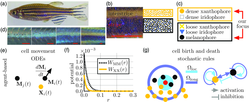
Figure 1: Motivating biological example. (a) Wild-type zebrafish feature stripe patterns in their skin. (b) Dark stripes and gold interstripes consist of several different types of brightly colored pigment cells. (c) For the purposes of this manuscript, we focus on melanophores and dense xanthophores, following the approach in [21]. (d) Over the course of several months, these cells organise sequentially into stripes and interstripes from the center of the fish body outward [10]. (e) The agent-based model (ABM) [21] that serves as the basis of our work describes how patterns arise through cell proliferation, competition, and movement. Cell movement is governed by ordinary differential equations (ODEs). (f) These ODEs account for cell–cell repulsion through potential functions, which describe melanophore–melanophore ($W_{\text{MM}}$) and xanthophore–xanthophore ($W_{\text{XX}}$) interactions as a function of their pairwise distance $r$. (g) The ABM [21] accounts for changes in cell number using stochastic discrete-time rules, which have the overarching form of short-range activation and long-range inhibition [22, 23, 19, 14, 24, 21]. These rules specify that a new melanophore appears at a randomly selected location (red) when there are more melanophores than dense xanthophores locally (in the blue disk) and more dense xanthophores than melanophores at long range (in the purple annulus). Red scale bar is $2$ mm in (b) and $250$ micrometers ($\mu$m) in (d). Images (a, b) adapted from Fadeev et al. [25] and licensed under CC-BY $4.0$ (https://creativecommons.org/licenses/by/4.0/); we added the text and red bar in (b). Image (d) adapted from Frohnhöfer et al. [10] and licensed under CC-BY $3.0$ (https://creativecommons.org/licenses/by/3.0/); published by The Company of Biologists Ltd.

Data-driven mathematical models can help uncover the drivers of zebrafish pattern formation and other biological phenomena exhibiting self-organization by identifying important phase transitions, isolating the effects of specific processes such as cell division, and providing hypotheses that can guide the design of in vivo experiments [26, 27, 28, 29]. Different modelling frameworks yield insight at the population or individual level, depending on how they represent members of a group. One modelling approach involves tracking how the position of each individual changes in time. These so-called “discrete” systems include center-based models [30, 31], cellular automata [32, 33], cellular Potts models [34, 35], and vertex models [36, 37]. Within the setting of zebrafish patterning, agent-based models (ABMs) have been developed that restrict cells to occupy certain locations “on-lattice” [38, 39, 40] or allow them to roam freely, “off-lattice”, in the domain [41, 42, 21, 43]. Due to their ability to work on the same length scales as empirical data, ABMs provide an intuitive connection to experiments and allow for detailed predictions about how interactions between agents drive group behaviours. However, ABMs can be prohibitive to simulate when the number of individuals is large, and understanding their long-time behaviour under alternative rules and parameters relies on extensive computation [44].

A second modelling approach uses continuous functions to represent the “average” density of agents in a collective, with their dynamics governed by a partial differential equation (PDE) in space and time. Continuous models, including reaction-diffusion equations, Boltzmann-like kinetic equations, and integro-differential equations (IDEs), typically cannot resolve individuals and, instead, track the ensemble average (EA) behaviour of a population. However, these models are more amenable to mathematical analysis and more readily provide insight into long-term behaviour than discrete frameworks do [45, 46]. For example, changes in patterning may arise because of Turing-like instabilities [22, 47, 48] or due to alterations in physically-based interactions such as cell–cell adhesion [49, 41, 50, 51, 52, 7]. In the case of zebrafish patterns, researchers have applied a wide swath of continuous models—including reaction-diffusion equations [38, 53, 54, 14, 19] and non-local PDEs [55, 56, 57, 7]—to better understand cell dynamics.

Despite the differences between discrete and continuous approaches, it is possible to establish a mathematical link between these representations in the limit of infinite individuals. This procedure, known as “coarse-graining”, derives differential equations from a given discrete model and yields information about its EA behaviour [58, 59, 60, 61, 62, 63]. For example, the authors in [64, 65, 66] derive logistic IDEs from stochastic processes that describe the birth and death of individuals undergoing Darwinian evolution via natural selection in the limit of large numbers. Coarse-grained descriptions become inaccurate when relatively few individuals are present, however, as is the case during early stages of pattern formation in zebrafish. Many approaches also neglect potentially important spatial correlations between cells—caused, for instance, by division or competition—that may play a critical role in pattern dynamics [67, 68, 69, 70, 71, 72, 54]. Consequently, it can be difficult to justify coarse-graining in biologically relevant settings. Nevertheless, we expect that it may be possible to correct for differences between continuous and discrete approaches, as both depict the same biological mechanisms and yield nearly indistinguishable results in the limit of an infinite number of agents.

We tackle this challenge by developing a pipeline to minimise spatio-temporal discrepancies between discrete and continuous models in settings with biologically relevant, dynamic cell numbers. We apply our approach to a case study motivated by stripe formation in zebrafish skin. The models that we consider in §2 account for cell movement and birth according to biologically inspired rules (Fig. 1) [21, 43]. As the continuous-model solutions do not capture the time scale at which biologically meaningful ABM solutions evolve, we introduce scaling parameters into the continuous framework and fit their values to EA ABM data. We demonstrate the robustness and effectiveness of this procedure in §3 for cases in which we isolate the respective time scales of cell movement and birth. However, we find that combining the two effects into a “full” model does not necessarily produce an accurate framework. This highlights the importance of capturing the interplay between different mechanisms when linking discrete and continuous models.

2 Mathematical models and methods

Following previous ABMs of pattern formation in zebrafish, we assume (1) migration is governed by repulsive forces between pigment cells and (2) non-local interactions inform cell birth in a two-dimensional ($2$D) plane [21, 43, 42]. While the models inspiring our work also include interactions between melanophores and xanthophores [42, 21], we restrict to one cell type at a time. We present our results for black melanophores in §3, and—as a means of demonstrating the flexibility of our methodology—apply the same approach to dense xanthophores in Supplementary Information (SI). Considering a single cell type masks biological complexity, since multiple populations interact to produce stripe patterns in vivo; see Fig. 1. However, in this manuscript we aim to develop a method for linking continuous and discrete models in biologically relevant scenarios with relatively low and highly dynamic cell numbers as a precursor to future work with added biological complexity. Basing our work on zebrafish allows us to illustrate the utility of our approach with biologically meaningful spatial and temporal units, providing interpretations of our parameters and equations in relation to experimentally measurable quantities. As we discuss in §4, we plan to extend our pipeline to multiple cell types in future work.

In §2.1, we develop our ABM for cell migration and derive its continuous counterpart. Subsequently, in §2.2, we introduce our discrete model for cell birth and develop a corresponding continuous IDE model. We present our full models of migration and proliferation in §2.3. Lastly, we present our approach to estimating scaling parameters in our continuous models from EA ABM data in §2.4. Throughout this section, we refer to:

$$\Omega\subset\mathbb{R}^{2} =\text{domain of the simulation with spatial units of millimeters (mm),}$$

$$\mathbb{R}^{2}\ni\textbf{M}_{i}(t) =\text{coordinates of the center of the $i^{\text{th}}$ melanophore at $t$ days in our discrete models,}$$

$$\mathbb{N}\ni N_{\text{M}}(t) =\text{total number of melanophores present at time $t$ days, and}$$

$$\mathbb{R}_{\geq 0}\ni M(\textbf{x},t) =\text{density of melanophores at position $\textbf{x}$ and time $t$ in cells/mm${}^{2}$,}$$

with the exception of Fig. 7 where we consider a one-dimensional ($1$D) domain; there $M(x,t)$ is the number density of melanophores in cells/mm. Because it appears several times, we define the indicator function $\mathds{1}_{\{\text{condition}\}}$ here, as:

$$\mathds{1}_{\{\text{condition}\}}(x) =\begin{cases}1,&\text{if $x$ satisfies the rule specified by ``condition"},\\ 0,&\text{otherwise,}\end{cases}$$ (1)

where “condition” depends on the model rule and cell interaction, as we discuss next.

2.1 Models of migration

Our ABM for cell movement tracks the position, $\textbf{M}_{i}(t)$, of each cell, indexed by $i\in\{1,\ldots,N_{M}\}$, at time $t\geq 0$. The movement of each melanophore depends on its interactions with surrounding melanophores, leading to a system of overdamped Langevin equations:

$$\frac{\text{d}\textbf{M}_{i}}{\text{d}t} \approx\textbf{F}^{(i)}_{\text{int}}=-\sum_{j=1,j\neq i}^{N_{\text{M}}}\nabla W_{\text{MM}}^{c}(\textbf{M}_{i}-\textbf{M}_{j}).$$ (2)

Here $\textbf{F}^{(i)}_{\text{int}}$ is the net force arising from all cell–cell interactions according to the potential:

$$W_{\text{MM}}(\textbf{r}) =R_{\text{MM}}e^{-|\textbf{r}|/\omega_{\text{MM}}},$$ (3)

where r is the inter-particle distance, as in [42, 21]; see Fig. 1(f) and Table 1 for parameter values. We use the notation $\nabla W_{\text{MM}}^{c}(\textbf{r})=\nabla W_{\text{MM}}(\textbf{r})\,\mathds{1}_{\{|\textbf{r}|~{}<~{}0.2~{}\text{mm}\}}(\textbf{r})$ to account for a finite interaction radius of $0.2$ mm, and set $N_{\text{M}}(t)=N_{\text{M}}$ when there is no cell birth.

The associated continuous model describes the melanophore density, $M(\textbf{x},t)$. Integrating $M(\textbf{x},t)$ over a bounded region yields the total number of melanophores within that area at time $t$. Following the coarse-graining procedure in [73, 61, 74], we obtain the PDE below:

$$\frac{\partial M}{\partial t} =\alpha_{\text{MM}}\nabla\cdot\Big{(}M\nabla W_{\text{MM}}^{c}\star M\Big{)},$$ (4)

where the force $\nabla W_{\text{MM}}^{c}$ is the same as in Eqn. (2) and $\star$ is the convolution operator [42, 21]. The parameter $\alpha_{\text{MM}}$ in Eqn. (4) is not inherent to the coarse-graining procedure; instead, we introduce it to account for possible differences between the time scales of the discrete and continuous models. Indeed, simulating the PDE with $\alpha_{\text{MM}}=1$ does not always capture the ABM dynamics; see Fig. 2. The individual and EA ABM results demonstrate that cells disperse until they are about $55$–$115$ $\mu$m apart at $t=150$ days. The PDE with $\alpha_{\text{MM}}=1$, however, predicts that cells travel about $250$ $\mu$m further in the same time period. Additionally, the PDE cell density is lower than the EA ABM density near the center of the domain, implying that cells are more separated there. The continuous solution at earlier times more closely resembles the EA ABM result at $t=150$ days, however, which suggests that the time scale of the PDE is faster than that of the discrete model. Thus, a non-unitary value of $\alpha_{\text{MM}}$ is likely to produce a better match between the discrete and continuous solutions. To our knowledge, the value of $\alpha_{\text{MM}}$ cannot be derived a priori. Instead, we develop an approach for estimating its value based on ABM data in §2.4.

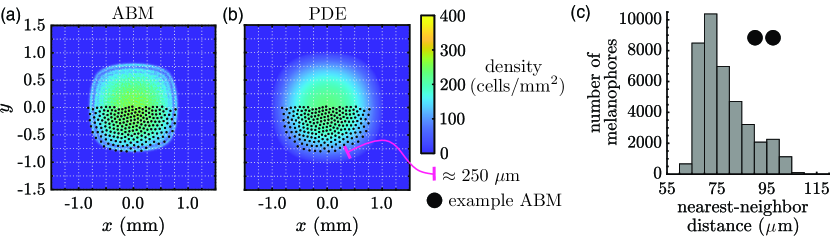
Figure 2: The PDE for cell migration does not accurately describe the EA ABM result when its scaling parameter $\alpha_{\text{MM}}$ is set to unity. (a) To compute our EA ABM result, we solve Eqn. (2) using an initial condition of $400$ melanophores placed uniformly at random in a $1$ mm $\times$ $1$ mm square; group cell positions in a $240$ $\times$ $240$ histogram; and average such data over $10^{4}$ ABM realizations. (b) We compute the corresponding PDE solution by simulating Eqn. (4) with $\alpha_{\text{MM}}=1$ from a uniform density of $400$ cells/mm² in the same square region. The ABM and PDE solutions use the same potential (given by Eqn. (3) with parameters in Table 1). We overlay an example ABM realization for comparison; the results demonstrate that the support of the PDE is larger than that of the ABM by about $200$ to $250$ $\mu$m. Because melanophore–melanophore distances have been measured to be roughly $50$ $\mu$m in vivo [75] and stripes are only about $7$–$12$ cells wide [14], this is a large difference. (c) The distribution of nearest-neighbor distances across $100$ ABM realizations demonstrates that cell–cell separation ranges from roughly $60$ to $100$ $\mu$m. Based on visual inspection of the graphs, nearest-neighbor distances appear inversely proportional to the EA cell density. In (a)–(c), we show results at $t=150$ days.

2.2 Models of cell birth

Our ABM for cell birth consists of stochastic, discrete-time rules which we adapt from [21]. Specifically, at each time step (i.e., day) in a simulation we select $N_{\text{bir}}\in\mathbb{N}$ locations uniformly at random from $\Omega$ and evaluate them synchronously for possible cell birth. Each selected location, z, represents the position of a precursor cell that may differentiate into a melanophore based on the signals that it receives. The conditions for melanophore birth in the ABM [21] depend on both neighboring melanophores and dense xanthophores, as we show in Fig. 1(g). Since we restrict to one population in this manuscript, we simplify the rules from [21]; see SI for details. In particular, a new melanophore emerges at position z according to the rule:

$$\underbrace{\sum_{i=1}^{N_{\text{M}}}\mathds{1}_{\{\textbf{M}_{i}~{}\in~{}\Omega_{\text{loc}}^{\textbf{z}}\}}(\textbf{M}_{i})\geq 1}_{\text{short-range activation}}~{}~{}\text{and}~{}~{}\underbrace{\sum_{i=1}^{N_{\text{M}}}\mathds{1}_{\{\textbf{M}_{i}~{}\in~{}\Omega_{\text{loc}}^{\textbf{z}}\}}(\textbf{M}_{i})~{}<c^{+}_{\text{ABM}}}_{\text{overcrowding prevention}}~{}~{}\longrightarrow~{}~{}\text{melanophore appears at {z}},$$ (5)

where $c^{+}_{\text{ABM}}\in\mathbb{N}$, and

$$\Omega_{\text{loc}}^{\textbf{z}} =\text{disk centered at $\textbf{z}$ with radius $75$ $\mu$m}.$$ (6)

According to Eqn. (5), new cells appear near existing melanophores until the maximum number of cells—namely, $c^{+}_{\text{ABM}}$—in $\Omega_{\text{loc}}^{\textbf{z}}$ is reached. As in [21] and based on estimations of data in [14, 75], we set $c^{+}_{\text{ABM}}=6$ cells. While Eqn. (5) is deterministic, stochasticity enters our ABM through our $N_{\text{bir}}$ randomly selected positions $\{\textbf{z}\}$.

We do not know of existing methods for rigorously deriving continuous models of cell birth from off-lattice ABMs with our noise structure. Instead, taking a phenomenological modelling approach, we reason that the rate at which the melanophore density increases is uniform and proportional to $N_{\text{bir}}$ within regions where the overcrowding and short-range activation conditions are satisfied, and zero otherwise. This leads to the continuous model below:

$$\frac{\partial M}{\partial t}(\textbf{x},t) =\gamma N_{\text{bir}}{\mathds{1}_{\left\{1<\int_{\Omega_{\text{loc}}^{\textbf{x}}}M(\mathbf{y},t)~{}d\mathbf{y}~{}<~{}c^{+}\right\}}}(\textbf{x},t),$$ (7)

where $c^{+}$ is the continuous equivalent of the density-limiting parameter $c^{+}_{\text{ABM}}$ in Eqn. (5); $N_{\text{bir}}$ has the same value as in our corresponding ABM; and $\gamma\in\mathbb{R}^{+}$ is a scaling parameter that we introduce which results in an upper bound on the number of cells born per unit time of $\gamma N_{\text{bir}}|\Omega|$. Equation (7) is a heuristic continuous description of the ABM dynamics of non-local proliferation with overcrowding avoidance, and we overview our approach to estimating the values of $c^{+}$ and $\gamma$ in §2.4.

2.3 Full models of cell movement and birth

We combine our descriptions of cell movement and proliferation to form our full discrete and continuous models. For our full ABM, we move cells according to Eqn. (2) and then introduce new agents based on Eqn. (5) at each simulated day; see SI for details. For our continuous model, we combine the terms related to movement and birth, such that the cell density evolves according to:

$$\frac{\partial M}{\partial t}(\textbf{x},t) =\alpha_{\text{MM}}\nabla\cdot\Big{(}M\nabla W_{\text{MM}}^{c}\star M\Big{)}+\gamma N_{\text{bir}}{\mathds{1}_{\left\{1~{}<~{}\int_{\Omega_{\text{loc}}^{\textbf{x}}}M(\mathbf{y},t)~{}d\mathbf{y}~{}<~{}c^{+}\right\}}}(\textbf{x},t),$$ (8)

where the parameters $\alpha_{\text{MM}}$, $\gamma$, $N_{\text{bir}}$, and $c^{+}$ have the same interpretations as in §2.1 and §2.2. Importantly, by assuming that these parameters have the same interpretations, we are assuming that migration and proliferation are additive, so that combining them has no extra influence. Our modular fitting approach, which we discuss below and summarize in Fig. 3, allows us to evaluate this assumption and better understand the interplay of these two mechanisms.

2.4 Parameter estimation procedure

As we show in Fig. 3, we adopt a modular approach for parameter estimation by fitting values related to cell migration and birth separately. This allows us to probe each mechanism in detail and determine its effects on group behaviour. Additionally, by using their parameter estimates in a combined setting, we can investigate the interplay between these processes, as we discuss in §3. Here, we identify the scaling parameters—$\alpha_{\text{MM}}$ in Eqn. (4) and $\{\gamma,c^{+}\}$ in Eqn. (7)—that minimise the sum of squared differences (hereafter referred to as the “$L^{2}$ error”) between the continuous and EA discrete solutions over time and space; see Fig. 3. This nonlinear least-squares problem is equivalent to maximum likelihood parameter estimation when the densities produced from the ABM simulations are independent, identically distributed normal random variables with constant variance and mean equal to the continuous solution. We overview our methods here; for details and parameter values, see SI and Table 1.

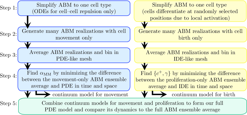
Figure 3: Our pipeline for matching the solutions of continuous and discrete models and identifying how cell movement and birth interact in both settings. We first isolate the discrete-model terms from [21] corresponding to movement (left column) and birth (right column) and simplify them to consider only one cell type. We then produce multiple realizations of our ABMs, sorting the cell locations into a grid of $N_{\text{hist}}\times N_{\text{hist}}$ voxels to yield the EA discrete model results. We simulate our continuous model for cell movement (respectively cell birth) and compare it on the same spatial mesh, with values of $\alpha_{\text{MM}}$ (respectively $c^{+}$ and $\gamma$) obtained from a least squares optimization approach; see SI for details. Finally, we combine the fitted movement and birth models to produce our full continuous model. While extension of this pipeline to fit all three parameters simultaneously is straightforward, fitting separately allows us to better understand the effects of cell movement and birth in discrete and continuous frameworks.

We consider biologically meaningful time scales (i.e., days), length scales (i.e., mm), and cell densities and stress empirical units throughout our results. This choice supports future studies that may treat pattern formation with multiple cell types. Throughout our simulations, we consider a domain of size $3$ mm $\times$ 3 mm (with one $1$D exception in Fig. 7). We implement four initial conditions to extract common features of cell interactions from different geometric scenarios: a square region of melanophores in the center of the domain (“Box”), a single stripe of melanophores (“Stripe”), two rectangular regions of melanophores (“Offset rectangles”), and two melanophore stripes (“Two stripes”). We initialise individual ABM simulations by sampling cell positions uniformly in these regions for each respective initial condition, and initialise our continuous models by setting the cell density uniformly equal to the estimated biological density of $400$ cells/mm² within the same regions [21]. To compare ABM results directly with the cell density from our continuous models, we obtain an EA distribution by simulating many ABM realizations, sorting all the cell locations into a grid of $N_{\text{hist}}$ $\times$ $N_{\text{hist}}$ voxels (or $N_{\text{hist}}$ $\times$ $1$ voxels in $1$D), and normalizing by the number of simulations and the voxel area each day.

We solve our continuous models with explicit approaches: we use a first-order finite volume scheme for the migration model (Eqn. (4)), a forward Euler method for the proliferation model (Eqn. (7)), and a combined scheme for the full framework (Eqn. (8). We simulate the continuous models on a $N_{\text{bin}}$ $\times$ $N_{\text{bin}}$ mesh and, to match with EA ABM solutions, record the average cell density at each day on a (possibly coarser) grid of $N_{\text{hist}}$ $\times$ $N_{\text{hist}}$ voxels. We compute continuous model parameters by minimizing either the $L^{2}$ error between the continuous and EA ABM results across time or (for the cell birth case) by matching the total cell count of the two data sets. When we consider cell birth, we simulate our models with different values of $N_{\text{bir}}$ and estimate parameters by minimizing the sum of the errors across these $N_{\text{bir}}$ values. We fit parameters related to cell proliferation sequentially—that is, we determine the optimal value for $c^{+}$ before $\gamma$. We verify in $1$D that sequential and simultaneous estimation does not lead to significant difference in parameter values; see SI.

3 Results

We now present our results linking discrete and continuous models of cell migration (§2.1), birth (§2.2), and migration and birth (§2.3). We first isolate each interaction process, separately identifying the values of $\alpha_{\text{MM}}$ in Eqn. (4) and $\{\gamma,c^{+}\}$ in Eqn. (7). As we note in §2.4, this choice allows us to extract the distinct effects of each mechanism. We then determine how this simplification affects the ability of the full continuous framework, given by Eqn. (8), to approximate EA ABM solutions. By considering different initial conditions, we demonstrate the robustness of our fitting procedure. Our results show how the time scales of proliferation and movement in our continuous model may depend on numerical implementation and the frequency of stochastic cell birth controlled by $N_{\text{bir}}$. Moreover, our modular fitting approach highlights important considerations to account for in more general systems where agents are moving and changing in number.

3.1 Cell migration

We estimate $\alpha_{\text{MM}}$, the scaling parameter that controls the dynamics of melanophore movement. Figure 4(a) presents the values of $\alpha_{\text{MM}}$ that minimise the squared $L^{2}$ error between the continuous solution of Eqn. (4) and EA ABM results for our four initial conditions (see §2.4 and SI). In each case, the optimal value of $\alpha_{\text{MM}}$ is positively correlated with our PDE mesh resolution, i.e., greater values of $\alpha_{\text{MM}}$ are associated with larger $N_{\text{bin}}=N_{\text{hist}}$ values. This unitless parameter appears to converge to around $0.60$ to $0.66$ as the mesh resolution increases. There is at most a $2.5$% relative difference between the values of $\alpha_{\text{MM}}$ that we find when $N_{\text{bin}}=240$ versus when $N_{\text{bin}}=480$ for our Box initial condition. These results suggest that $\alpha_{\text{MM}}$ is independent of the mesh resolution when the latter contains at least $240$ $\times$ $240$ voxels, corresponding to a mesh spacing of $12.5$ $\mu$m. As we show in Fig. 2(c), melanophores tend to separate by between $60$–$100$ $\mu$m in our ABM results, so this mesh spacing is less than one quarter of the typical distance between agents.

At each mesh resolution in Fig. 4(a), the estimated optimal value of $\alpha_{\text{MM}}$ does not appear to depend greatly on the initial condition. For example, in the case of a mesh with $N_{\text{bin}}=N_{\text{hist}}=240$, the maximum relative difference between the four parameter values is at most $6.5$%. This similarity suggests that there is an inherent time scale at which migratory melanophore–melanophore interactions occur. Figure 4(b), which presents the $\log L^{2}$ error for $N_{\text{bin}}=240$ as a function of $\alpha_{\text{MM}}$, further supports this conclusion. Although the errors associated with different initial conditions can vary by an order of magnitude, the minimum value of each (roughly convex) curve appears nearly identical and is located near the values shown in Fig. 4(a).

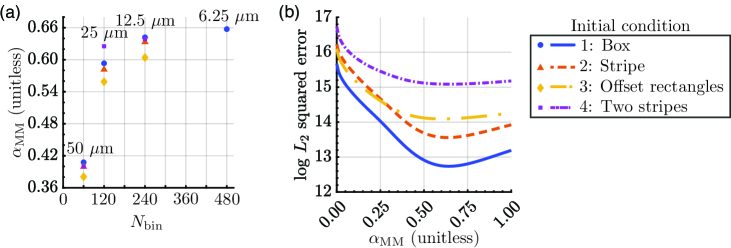
Figure 4: The optimal PDE scaling parameter for movement depends on the mesh resolution but appears to converge. (a) A scatter plot of the numerically optimised value of $\alpha_{\text{MM}}$ from Eqn. (4) as a function of the mesh resolution, $N_{\text{bin}}$, demonstrates that this scaling parameter is correlated with the mesh resolution, but appears to converge at sufficiently high (i.e., $N_{\text{bin}}\geq 240$) detail. (We omit $95$% confidence intervals because these are so narrow that they are difficult to see.) (b) Plotting the $\log L^{2}$ error, given by Eqn. (S8) of the SI, as a function of $\alpha_{\text{MM}}$ with $N_{\text{bin}}=240$ for each initial condition suggests that the values in (a) are optimal. As we show in Fig. 2(c), melanophores are typically separated by more than $60$ $\mu$m in our movement-only ABM simulations—over four times the voxel width in a grid with $N_{\text{bin}}=240$. See §2.4 and SI for numerical details.

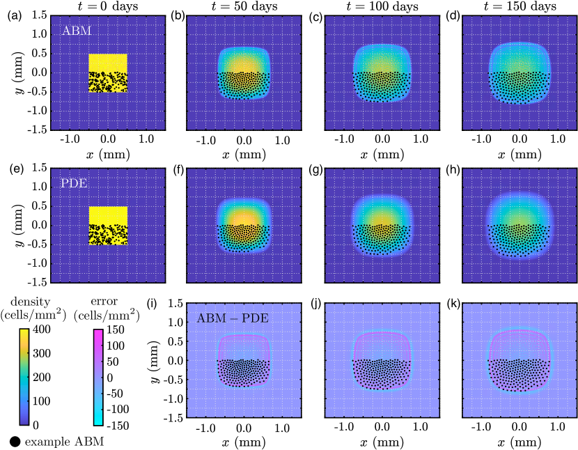
Figure 5: Melanophore movement models with our Box initial condition. We present (a)–(d) snapshots of the EA cell density (cells/mm²) across $10^{4}$ ABM realizations, (e)–(h) the corresponding PDE results using the optimal value of $\alpha_{\text{MM}}$ for a mesh resolution of $N_{\text{bin}}$ = 240, and (i)–(k) the error between the PDE and EA ABM densities. We overlay cell positions for one example ABM simulation (black points) as a visual guide; we show roughly half of the region occupied by these cells. A difference in cell density of $150$ cells/mm² in a given voxel corresponds to about $0.0234$ cells for this choice of mesh resolution.

Figure 5 presents snapshots of the EA ABM results across $10,000$ realizations of Eqn. (2) and the optimised PDE solution associated with the Box initial condition. The first row shows the expansion in time of the EA ABM support, i.e., the area occupied by the cells, due to melanophore–melanophore repulsion. For more intuition, we superimpose the cell positions from one ABM realization on our number-density results in this figure and throughout the manuscript. In all cases, we crop out approximately the upper half of cell positions. Visual inspection of cell positions in Fig. 5 suggests that melanophore–melanophore distances increase near the edge of the collective. Similarly, the speed at which the support expands appears to slow down for the EA ABM result, consistent with melanophores experiencing weaker forces from comparatively distant cells in this region.

We also observe in Fig. 5(a)–(d) that a band of high cell density emerges around the edge of the support which surrounds a ring-like region of low density. These bands may result from the combined effects of cell–cell repulsion and the fine mesh resolution that we use to sort agent positions in the EA solution. Repulsion causes cells at the edge of the collective to travel towards empty regions, while more centrally located agents move slower due to the balance of forces from their neighbors. When repulsion separates cells by distances greater than the mesh resolution, we expect regions of low density within the solution support to appear. These oscillatory bands should become less evident when the repulsive potentials in Fig. 1(f) exhibit shallower gradients, as this permits cells to cluster more closely. As we discuss in SI, the forces acting on xanthophores are about an order of magnitude smaller than those for melanophores, and we indeed observe less pronounced bands there.

We present snapshots of the continuous model, Eqn. (4), under our estimated value of $\alpha_{\text{MM}}$ in Fig. 5(e)–(h). This PDE solution captures the dynamics of our example ABM realization significantly better than the case in Fig. 2(b), when $\alpha_{\text{MM}}=1$. However, unlike the EA ABM result, the PDE does not exhibit bands of high and low cell density. This discrepancy can be further appreciated in Fig. 5(i)–(k), which presents snapshots of the pointwise difference between the PDE and EA ABM solutions. Here positive values indicate that the discrete solution is larger than the continuous one. The lack of bands in the PDE setting is likely because the mean-field assumption used to derive the continuous system is invalid where density is low. We do not expect this discrepancy to be as pronounced in models that include cell birth, as this mechanism increases density; see §3.3. Moreover, the PDE support expands faster than that of the ABM. This result is likely due to our choice of error function to fit $\alpha_{\text{MM}}$. Specifically, this parameter is biased towards values that produce accurate approximations in the bulk as these regions have a larger contribution to the $L^{2}$ norm. Since we have already determined the assumptions underlying the continuous model break down in low density regions, however, we choose to fit to the bulk of the cell density and focus on the $L^{2}$ difference.

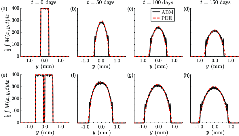
Figure 6: Melanophore movement models with our Stripe and Two stripes initial conditions. (a)–(d) We present snapshots of the column-averaged cell density (cells/mm², black solid line), generated from $5\times 10^{3}$ ABM realizations for the Stripe case, alongside the corresponding PDE solution (dashed red line) under a mesh resolution of $N_{\text{bin}}=240$ and our optimised value of $\alpha_{\text{MM}}$. (e)–(f) Similarly, we show snapshots of the column-averaged density, generated from $10^{3}$ ABM realizations for the Two stripes case, and the corresponding PDE solution. The $2$D solutions are nearly uniform in the $x$-direction (data not shown).

To demonstrate that our observations for the Box case are consistent across initial conditions, we compare the EA ABM and PDE dynamics for the Stripe and Two stripes initial conditions in Fig. 6. (See Supplementary Fig. 2 for the Offset rectangles initial condition.) In Fig. 6(a)–(d), the column-averaged PDE solution, i.e., the solution average over the $x$ variable, has a larger support than that of the EA ABM and does not exhibit oscillatory bands. (Comparing column averages is justified because both results are nearly uniform along the $x$-axis.) Nevertheless, the continuous solution closely approximates the EA ABM density, particularly in regions where the latter is high. After about $t=25$ days, for example, the maximum pointwise difference between the column-averaged solutions is no more than $80$ cells/mm². Both solutions invade empty space in time, and the speed of this travelling wavefront appears to slow as cells become more diffuse. For the Two stripes initial condition in Fig. 6(e)–(h), the ABM and PDE predict that cells move into the initially empty space between stripes to approach a characteristic profile also observed in the one-stripe case. The EA ABM model does not appear to form oscillatory bands in the interstripe region, corroborating our hypothesis that these bands are more likely to arise near the edge of the solution support.

3.2 Cell birth

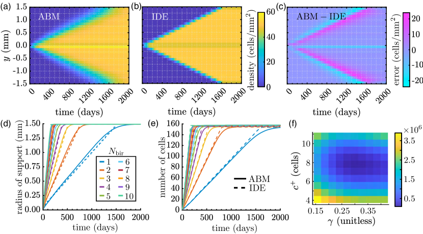
Figure 7: Melanophore birth models with a baseline initial condition of one cell at $y=0$ in a 1D domain. Results in (a)–(c) are for $N_{\text{bir}}=1$ position/day. (a) We compute the EA ABM result by simulating $10^{3}$ realizations of our ABM birth model, Eqn. (5), and binning cell positions in a histogram with $0.1$ mm-wide voxels (i.e., $N_{\text{hist}}=30$). (b) We use a finer mesh resolution to solve our corresponding IDE model (Eqn. (7)) before transferring results to the same histogram in (a) to perform parameter estimation. Here we show our IDE solution produced with optimal parameter values $c^{+}=7.592$ cells and $\gamma=0.2822$. (c) The difference between our discrete and continuous results highlights that the ABM support is wider than the PDE support. (d) This is also visible by comparing their mean radii of support in time. To compute the mean radius of support for the ABM at a given time, we find the most distant melanophore from $y=0$ for each simulation and average across these values. (e) Cell mass grows linearly in both models at first, but stochastic effects coupled with our overcrowding condition drive down the growth rate of the ABM as the domain fills with cells. (f) Plotting the squared $L^{2}$ space-time difference between the discrete and continuous densities, summed over all $N_{\text{bir}}$ values considered (namely $N_{\text{bir}}=1,...,10$), as a function of the density-limiting parameter $c^{+}$ and birth-rate scaling parameter $\gamma$ highlights its convex shape in $c^{+}$ and lesser sensitivity to $\gamma$. We compute this $L^{2}$ difference using a time step of $10$ days here, and our results are based on $10^{3}$ simulations for each $N_{\text{bir}}$ value. See SI for parameter values under alternative choices in our estimation process.

We identify the density-limiting parameter $c^{+}$ and growth rate $\gamma$ in our IDE model, Eqn. (7), by comparing with agent-based data from Eqn. (5). Importantly, the dynamics of discrete-model proliferation, unlike cell migration, involve stochasticity beyond the initial condition. To gain intuition, we thus start with 1D simulations: for each value of $N_{\text{bir}}\in\{1,2,\dots,10\}$, we compute the EA of $10^{3}$ ABM realizations from an initial condition in which a single melanophore is placed at the origin in a 1D domain. In Fig. 7(a) we show the EA result for $N_{\text{bir}}=1$ and the corresponding IDE model solution with the optimal values of $\gamma$ and $c^{+}$ in Fig. 7(b). The continuous solution appears to have a smaller radius of support than the EA ABM result at every time point; see Fig. 7(c). This result holds across all $N_{\text{bir}}$ values in Fig. 7(d). While the IDE predicts a piecewise linear growth of the total number of cells, the corresponding EA ABM result increases linearly before slowly saturating as the domain fills, as we depict in Fig. 7(e). This behaviour likely arises from our overcrowding condition that prevents cell densities from exceeding $c^{+}$. As the domain fills with cells, it becomes less likely to select a location z that satisfies the overcrowding condition in the ABM. This reduces the population growth rate at later times. In contrast, the IDE model specifies that the support increases by the same amount at each time step until it reaches the domain boundaries. As we discuss in §4, capturing discrete model behaviour more accurately at higher cell numbers may require replacing $\gamma$ in our IDE with a density-dependent function.

Our $1$D simulations provide a baseline case to test our estimation process. As we note in §2.4, we employ a sequential procedure, first fitting $c^{+}$ with $\gamma=|\Omega|^{-1}$ and then estimating $\gamma$ with $c^{+}$ fixed. In the 1D case, this leads to optimal values $c^{+}=7.592$ cells and $\gamma=0.2822$. If we instead estimate both parameters simultaneously, we find $c^{+}=7.430$ cells and $\gamma=0.2902$. This is a difference of about $2.1$% in $c^{+}$ and $2.8$% in $\gamma$, suggesting that sequential estimation reduces computational complexity without strongly affecting parameter values. To understand if a coarser discrepancy measure based only on cell numbers at each time is sufficient, we also fit $c^{+}$ and $\gamma$ by minimizing the squared difference in the total cell numbers over time (See Supplementary Table 3 for the resulting parameter values). The corresponding parameter estimates differ from the density-based case by approximately $1.2$% for and $c^{+}$ and $\gamma$, suggesting both error measures are reasonable. Both approaches also appear to exhibit similar sensitivity as parameters are varied (compare Figs.7(f) and Supplementary Fig. 1).

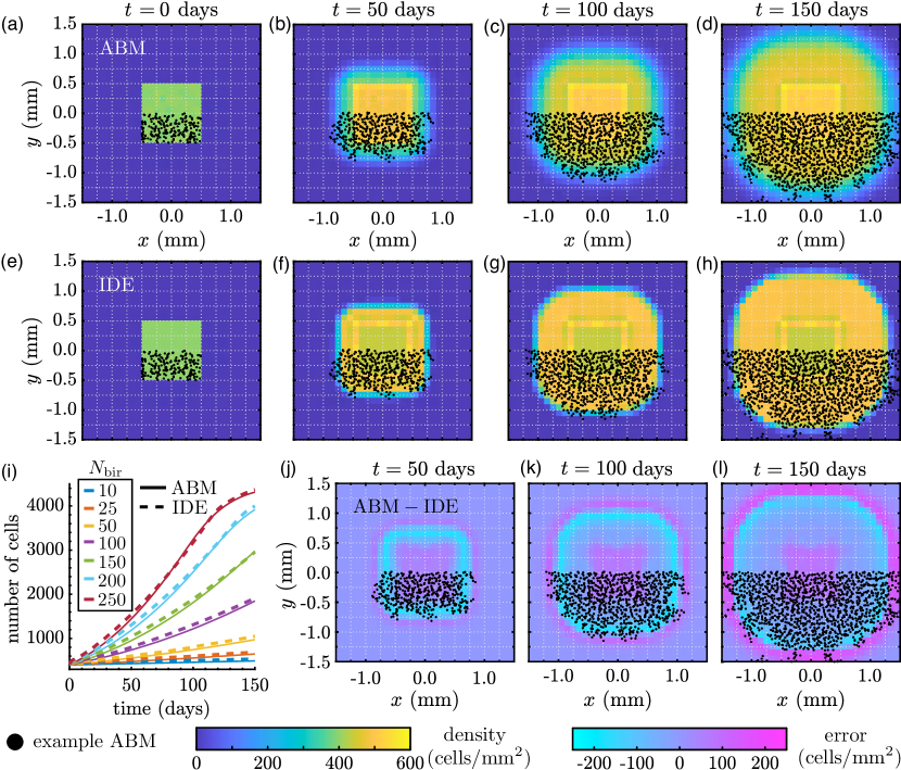
Figure 8: Melanophore proliferation models with our Box initial condition. Results in (a)–(h) and (j)–(l) are for $N_{\text{bir}}=150$ positions/day. We compute (a)–(d) the EA ABM result across $10^{3}$ simulations, and (e)–(h) the solution of our IDE model with optimal parameters $c^{+}=8.564$ and $\gamma=0.1274$. (i) Our continuous model captures the mean number of cells in our ABM simulations for different $N_{\text{bir}}$ values well across time. (j)–(l) As in the 1D case in Fig. 7, the difference between the IDE and EA ABM results demonstrates that the ABM support extends beyond the IDE support. To provide more intuition, we overlay roughly half of the cell positions from an example ABM simulation in (a)–(h) and (j)–(l). See Supplementary Fig. 3 and Supplementary Table 4 for corresponding simulations using our Offset rectangles initial condition.

Figure 8 and Supplementary Fig. 3, respectively, show that proliferation in 2D broadens the solution support from the Box and Offset rectangles initial conditions over time, and the IDE model accurately captures the total cell mass of the ABM system for all $N_{\text{bir}}$ values considered. Our estimated optimal values of $c^{+}$ and $\gamma$ for these two initial conditions differ by about $2.5$% and $0.31$%, respectively, suggesting that our estimation procedure is robust to the initial condition. We also highlight that a region of higher density forms at the edge of the initial condition’s support for both the ABM and IDE in Fig. 8(a)–(h). Indeed, if z is near the support boundary, $\Omega_{\text{loc}}^{\textbf{z}}$ covers only a fraction of the occupied domain, thereby meeting both conditions for birth. Conversely, the cell density at the center of the domain is comparatively low throughout time because the total number of cells contained within disks of size $\lvert\Omega_{\text{loc}}\rvert$ is already close to the threshold $c^{+}$. Interestingly, as in the 1D case with only proliferation, the ABM EA support is larger than that of the IDE solution, the reverse of the behaviour that we observed for cell migration in Fig. 5.

3.3 Cell movement and proliferation

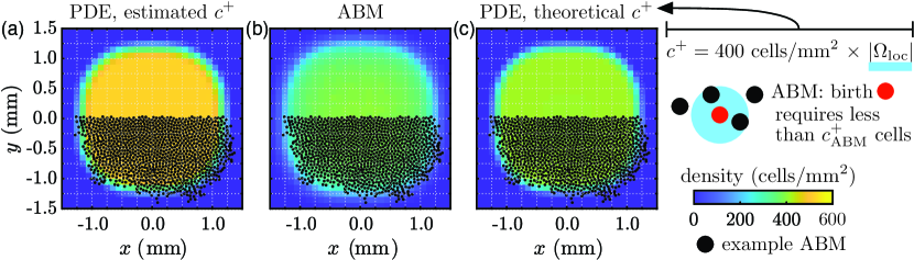
Figure 9: A modular approach to fitting parameters for cell movement and birth does not account for the interplay between these two mechanisms. We show results in (a)–(c) at $t=100$ days for $N_{\text{bir}}=150$ positions/day. (a) The solution of our full PDE model (Eqn. (8)) with the values of $\alpha_{\text{MM}}$ and $\{c^{+},\gamma\}$ that we fit based on ABM simulations of cell movement and birth, respectively, captures the support of the ABM EA result, but not its density. (b) In comparison, the density for the full discrete model is roughly $400$ cells/mm². (c) By integrating this density, which is based on empirical estimates of melanophore–melanophore distances [75, 21], over an $\Omega_{\text{loc}}$-region, we find that $c^{+}\approx 7.0686$ cells. With this value of $c^{+}$, alongside the values of $\alpha_{\text{MM}}$ and $\gamma$ that we estimated for migration and birth individually, our PDE produces cell densities that more accurately represent the ABM dynamics.

To obtain a full continuous model, we may substitute our estimated values of the migration scaling parameter $\alpha_{\text{MM}}$, density-limiting parameter $c^{+}$, and birth-rate scaling parameter $\gamma$ into Eqn. (8). However, comparing this model to the dynamics of our full ABM shows that migration and proliferation have interwoven effects. To illustrate this phenomenon, we present a PDE solution with our optimal values of $\alpha_{\text{MM}}$, $c^{+}$, and $\gamma$ from §3.1 and 3.2 at $t=70$ days in Fig. 9(a). We observe that this PDE model produces a significantly higher cell density than its discrete counterpart in Fig. 9(b). This discrepancy occurs regardless of the value of $N_{\text{bir}}$, which influences the speed of cell birth. Related to this, we notice that the long-time cell density in our ABM results is much lower when both mechanisms operate simultaneously than it is when only birth occurs; compare Fig. 8(d) and Fig. 9(b). On the other hand, the inclusion of movement does not influence the long-time density of the continuous model solution; see the colorbar in Fig. 8(h) in comparison to the one in Fig. 9. Although we do not furnish these observations with an analytical explanation here, they demonstrate an interesting difference in how “adding” mechanisms or terms impact PDE and ABM dynamics.

While we could produce a more accurate continuous model of migration and proliferation by minimizing the $L^{2}$ error between the full PDE and ABM results to identify all three parameters, we instead employ a simpler theoretical argument. We notice that the parameter $c^{+}$ is largely responsible for controlling the maximum cell density over long time periods. (We determine this by integrating Eqn. 8 over space and identifying the steady-state dynamics; this analysis reveals that equilibrium is reached when the density within any neighborhood $\Omega^{\mathbf{x}}_{\mathrm{loc}}$ is below $c^{+}$.) In order to limit the maximum density to our estimated empirical value of $400$ cells/mm² [75, 21], we let $c^{+}=400|\Omega_{\mathrm{loc}}|\approx 7.0686$ cells. As we show in Fig. 9(c), using this value of $c^{+}$, alongside our previously fit values of $\alpha_{\text{MM}}$ and $\gamma$, produces PDE densities that are much closer to the corresponding ABM results. We thus fix $c^{+}=7.0686$ cells for the remainder of this manuscript, which allows us to highlight the time dynamics of our full PDE model in comparison to the EA ABM result with Box and Offset rectangles initial conditions in Fig. 10 and 11, respectively.

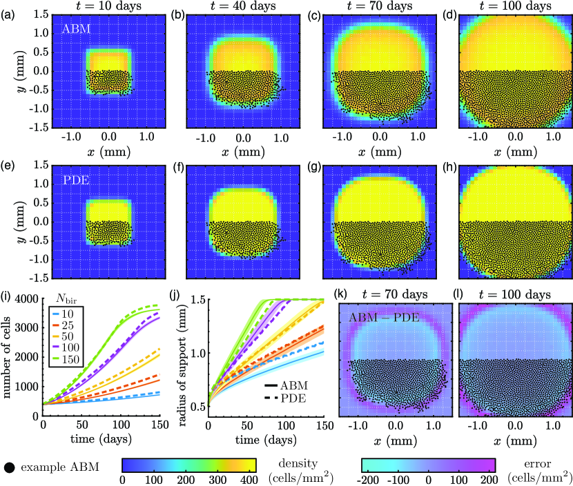
Figure 10: Melanophore movement and birth models with our Box initial condition. Results in (a)–(h) and (j)–(l) are for $N_{\text{bir}}=150$ positions/day. We (a)–(d) compute the EA ABM result using $10^{3}$ simulations, and (e)–(h) generate the PDE solution of Eqn. (8) with $c^{+}=7.0686$ cells and the values of $\alpha_{\text{MM}}$ and $\gamma$ that we estimated in §3.1 and §3.2, respectively. (i) The time evolution of the PDE cell mass agrees well with the mean number of cells for the ABM under different $N_{\text{bir}}$ values. (j) Depending on the time scales of migration and birth, the approximate PDE radius of support overtakes or trails the corresponding EA ABM result. We compute the radius of support for each ABM realization by finding the most distant cell from the origin at each time step; we then average these values across our simulations. In the PDE case, we find the furthest voxel with non-zero density from the origin based on the $L^{\infty}$ distance, after setting the density to zero if it is below single-digit precision of $10^{-7}$. (k)–(l) We show the difference between the PDE and EA ABM solutions from (a)–(h) at two sample times. We overlay cell positions form one ABM simulation to illustrate how the continuous and discrete solutions are related. In (i) and (j), shaded regions denote plus or minus one standard deviation of the EA ABM solution.

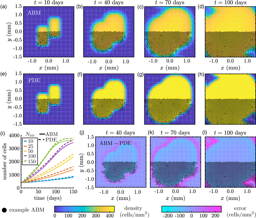
Figure 11: Melanophore movement and birth models with our Offset rectangles initial condition. Results in (a)–(h) and (j)–(l) are for $N_{\text{bir}}=150$ positions/day. As in Fig. 10, we show (a)–(d) the EA ABM result across $10^{3}$ simulations; (e)–(h) the corresponding PDE solution with $c^{+}=7.0686$ cells and the values of $\alpha_{\text{MM}}$ and $\gamma$ that we estimated in §3.1 and §3.2, respectively; (i) the PDE cell mass in time compared to the mean number of cells across $10^{3}$ ABM simulations for different $N_{\text{bir}}$ values; and (j)–(l) the difference between the PDE and EA ABM solutions from (a)–(h). To provide more intuition, we overlay some cell positions from one ABM simulation.

As we discussed in §3.1 and 3.2, the continuous solution support extends more slowly than that of our discrete model in a proliferation-only setting, but overestimates it in the case with migration alone. We thus expect that combining these mechanisms in our full model may balance these two errors, resulting in a more accurate continuous description. Figure 10(i), which depicts the time evolution of the estimated radius of support for the PDE and EA ABM results, supports this conclusion. When $N_{\text{bir}}$ is small, the solution support of the PDE surpasses that of the ABM solution, reflecting an increase in the time scale of proliferation. Conversely, the PDE solution extends beyond the ABM result for large values of $N_{\text{bir}}$. At intermediate values (i.e., $N_{\text{bir}}=50$ positions/day), the EA ABM and PDE dynamics agree for longer time periods. Figures 10 and 11 demonstrate that combining movement with proliferation also dissipates the oscillatory bands that we observed for movement alone in Fig. 5. Furthermore, the EA ABM and PDE solutions exhibit similar characteristic profiles without regions of high cell density around the edge of the initial condition support, in contrast to the birth-only model (Fig. 8).

4 Discussion

We presented a procedure for constructing experimentally interpretable continuous models of cell migration and birth when coarse-graining may not be possible or justified. Because mean-field approaches become more accurate in the limit of an infinite number of agents, we introduced and estimated scaling parameters in our continuous models to account for realistic—i.e., relatively small and changing—cell numbers. Stochastic non-local rules for cell birth and migration, based on the ABM [21], informed our continuous descriptions and allowed us to transfer biological length scales and units to the macroscopic setting. Throughout our work, we stressed matching the spatio-temporal behaviour of our continuous and discrete models. We adopted a modular approach by estimating parameters in cases with either movement or birth before considering both mechanisms simultaneously. This allowed us to examine the specific contributions of each mechanism to self-organization and provided insight into their interplay in discrete and continuous settings.

We observed that the solutions of our continuous models expand at a different rate than EA ABM results and feature smoother profiles. We produced more accurate descriptions of agent-based movement or birth by introducing and estimating parameters that adjust the time scale at which PDE solutions evolve. However, when we used the same parameter values in a continuous model of both cell migration and birth in §3.3, the PDE did not produce close estimates of the full ABM. Specifically, our full continuous model yielded larger long-time densities than the EA ABM results, motivating us to re-estimate the threshold value $c^{+}$ with a theoretical approach. This generated a more faithful continuous description and highlighted that the effects of movement and proliferation are not simply additive. We thus stress that parameters must be fit to data in which all mechanisms of interest act simultaneously, in order to capture their interplay. This is particularly crucial for contexts such as cancer biology, where continuous models sometimes struggle to predict tumour elimination because of the difficulty of accounting for the combined effects of cell migration, proliferation, and death [76].

Our results highlight how choices in numerical implementation affect parameter estimates and suggest several directions for future work that may improve our approach. For example, the optimal value of our parameter controlling the timescale of cell migration ($\alpha_{\text{MM}}$) appears to be independent of the initial condition and the mesh resolution that we used to construct PDE solutions, provided the latter is sufficiently refined. However, our continuous models more accurately represent ABM results within the bulk of the solution support because the $L^{2}$ norm more strongly penalises discrepancies there. In the future, other norms, such as the $L^{\infty}$ error, could be used to match the solution supports given by our discrete and continuous models. Replacing our birth-rate scaling parameter $\gamma$ with a density-dependent function—either through rigorous derivation or an equation-learning approach [77]—is another exciting future direction. In particular, because cell proliferation in the ABM involves selecting positions uniformly at random from the domain each day, the chance that we select a location z that permits birth appears to depend in a nonlinear way on the solution support. More generally, our computational study does not provide theoretical explanations for our parameter values, and we plan to build on the intuition that we established here to develop these arguments in the future.

To simplify our initial study, we considered the dynamics of one cell population (i.e., melanophores in the main text and xanthophores in SI), but pattern formation in zebrafish skin involves multiple cell types and longer-range interactions. Future work may extend our pipeline to construct more realistic continuous models with multiple cell types and interaction neighborhoods. Related to this, the initial conditions that we designed allowed us to make one-to-one comparisons between discrete- and continuous-model densities, but this may not always be possible. More realistic zebrafish models (i.e., [21, 43, 42, 40]) produce patterns that are more complicated than our box and stripe motifs. This means that ensemble-averaging stochastic ABM realizations may not retain information about the length scales inherent in patterns. For such cases, fitting parameters based on summary statistics (e.g., pair-correlation functions [78], pattern-simplicity scores [79], or persistent-homology approaches [80]) may be more useful, and we plan to address this in future work. These and other directions move us toward constructing interpretable, analytically tractable continuous models of self-organization, increasing our understanding of biological pattern formation more broadly.

Parameter	Value	Description and motivation
$R_{\text{MM}}$	$0.00124$ mm2/day	Strength of melanophore potential in Eqn. (3); based on [42, 21]
$\omega_{\text{MM}}$	$0.02$ mm	Melanophore interaction range in Eqn. (3); based on [42, 21]
$d_{\text{loc}}$	$0.075$ mm	Interaction range for proliferation in Eqn. (6); based on [21]
$N_{\text{bir}}$	Varies	Number of positions selected uniformly at random per day for possible cell proliferation in Eqns. (5) and (7)
$c^{-}$	$1$ cell	Lower bound for the number of cells in a short-range neighborhood for cell proliferation in Eqns. (5) and (7)
$t_{\text{final}}$	$150$ or $2,000$ days	Simulation end time ($150$ days in $2$D and $2,000$ days in $1$D)
$\Delta t_{\text{move}}$	$0.01$ or $0.1$ days	Time step for numerical implementation of Eqns. (2) and (S3)
$\Delta t_{\text{bir}}$	$1$ day	Time step for numerical implementation of cell birth in Eqns. (5) and (7)
$\Delta t_{\text{PDE}}$	$0.05$ days	Time step for numerical implementation of Eqns. (4), (8), and (S6)
$\Delta t_{\text{record}}$	$1$ day	Time step for recording data from model simulations
$N_{\text{sim}}$	Varies	Number of ABM realizations for computing EA cell densities
$N_{\text{hist}}$	$N_{\text{bin}}$ or $30$ voxels	Spatial discretization step for binning simulations results for comparison
$N_{\text{bin}}$	Varies	Spatial discretization step for solving our continuous models

Table 1: Model and simulation parameters. We note that $N_{\text{bir}}~{}\in\{10,25,50,100,150,200,250\}$ realizations for $2$D simulations and $N_{\text{bir}}\in\{1,2,3,4,5,6,7,8,9,10\}$ realizations for $1$D simulations. As we discuss in SI, $N_{\text{sim}}=5\times 10^{3}$ realizations for most of our ABM results with only cell movement and $N_{\text{sim}}=10^{3}$ for all of our ABM results that include cell birth. We set $N_{\text{hist}}=30$ voxels for any simulation including cell birth, and $N_{\text{hist}}=N_{\text{bin}}$ otherwise. (See figure captions for our $N_{\text{bin}}$ values.) The value of $R_{\text{MM}}$ (and $R_{\text{XX}}$, see SI) were reported as repulsion strengths (i.e., $R_{\text{MM}}/\omega_{\text{MM}}$) in [42].

Code availability

Our model and parameter-fitting code is publicly available on GitHub [81]. Supplementary figures and videos are available on Figshare at https://figshare.com/account/home#/projects/171234.

References

- [1] Mogilner A, Edelstein-Keshet L. A non-local model for a swarm. J Math Biol. 1999;38(6):534-70.
- [2] D’Orsogna MR, Chuang YL, Bertozzi AL, Chayes LS. Self-propelled particles with soft-core interactions: patterns, stability, and collapse. Phys Rev Lett. 2006;96(10):104302.
- [3] Cucker F, Smale S. Emergent behavior in flocks. IEEE Trans Autom Control. 2007;52(5):852-62.
- [4] Carrillo JA, Fornasier M, Toscani G, Vecil F. Particle, kinetic, and hydrodynamic models of swarming. In: Mathematical modeling of collective behavior in socio-economic and life sciences. Springer; 2010. p. 297-336.
- [5] Amack JD, Manning ML. Knowing the boundaries: Extending the differential adhesion hypothesis in embryonic cell sorting. Science. 2012;338:212-5.
- [6] Burger M, Francesco MD, Fagioli S, Stevens A. Sorting phenomena in a mathematical model for two mutually attracting/repelling species. SIAM J Math Anal. 2018;50(3):3210-50.
- [7] Carrillo JA, Murakawa H, Sato M, Togashi H, Trush O. A population dynamics model of cell-cell adhesion incorporating population pressure and density saturation. J Theor Biol. 2019;474:14-24.
- [8] Buttenschön A, Edelstein-Keshet L. Bridging from single to collective cell migration: A review of models and links to experiments. PLOS Comput Biol. 2020;16(12).
- [9] Tsai TYC, Garner RM, Megason SG. Adhesion-Based Self-Organization in Tissue Patterning. Annu Rev Cell Dev Biol. 2022;38:349-74.
- [10] Frohnhöfer HG, Krauss J, Maischein HM, Nüsslein-Volhard C. Iridophores and their interactions with other chromatophores are required for stripe formation in zebrafish. Development. 2013;140(14):2997-3007.
- [11] Irion U, Nüsslein-Volhard C. The identification of genes involved in the evolution of color patterns in fish. Curr Opin Genet Dev. 2019;57:31-8.
- [12] Parichy DM. Evolution of pigment cells and patterns: recent insights from teleost fishes. Curr Opin Genet Dev. 2021;69:88-96.
- [13] Kondo S, Watanabe M, Miyazawa S. Studies of Turing pattern formation in zebrafish skin. Philos Trans R Soc A. 2021;379(2213):20200274.
- [14] Nakamasu A, Takahashi G, Kanbe A, Kondo S. Interactions between zebrafish pigment cells responsible for the generation of Turing patterns. Proc Natl Acad Sci USA. 2009;106(21):8429-34.
- [15] Singh AP, Schach U, Nüsslein-Volhard C. Proliferation, dispersal and patterned aggregation of iridophores in the skin prefigure striped colouration of zebrafish. Nat Cell Biol. 2014;16(6):604-11.
- [16] Gur D, Bain EJ, Johnson KR, Aman AJ, Amalia Pasolli H, Flynn JD, et al. In situ differentiation of iridophore crystallotypes underlies zebrafish stripe patterning. Nat Commun. 2020;11(1):6391.
- [17] Hamada H, Watanabe M, Lau HE, Nishida T, Hasegawa T, Parichy DM, Kondo S. Involvement of Delta/Notch signaling in zebrafish adult pigment stripe patterning. Development. 2014;141(2):318-24.
- [18] Inaba M, Yamanaka H, Kondo S. Pigment pattern formation by contact-dependent depolarization. Science. 2012;335(6069):677-7.
- [19] Yamaguchi M, Yoshimoto E, Kondo S. Pattern regulation in the stripe of zebrafish suggests an underlying dynamic and autonomous mechanism. Proc Natl Acad Sci USA. 2007;104(12):4790–4793.
- [20] Kroll F, Powell GT, Ghosh M, Gestri G, Antinucci P, Hearn TJ, et al. A simple and effective F0 knockout method for rapid screening of behaviour and other complex phenotypes. eLife. 2021;10:e59683.
- [21] Volkening A, Sandstede B. Modelling stripe formation in zebrafish: an agent-based approach. J R Soc Interface. 2015;12(112):20150812.
- [22] Turing AM. The chemical basis of morphogenesis. Philos Trans R Soc Lond B. 1952;237(641):37-72.
- [23] Gierer A, Meinhardt H. A theory of biological pattern formation. Kybernetik. 1972;12(1):30-9.
- [24] Watanabe M, Kondo S. Is pigment patterning in fish skin determined by the Turing mechanism? Trends Genet. 2015;31(2):88-96.
- [25] Fadeev A, Krauss J, Frohnhöfer HG, Irion U, Nüsslein-Volhard C. Tight Junction Protein 1a regulates pigment cell organisation during zebrafish colour patterning. eLife. 2015;4:e06545.
- [26] Byrne HM. Dissecting cancer through mathematics: From the cell to the animal model. Nat Rev Cancer. 2010;10:221-30.
- [27] Gompper G, Winkler RG, Speck T, Solon A, Nardini C, Peruani F, et al. The 2020 motile active matter roadmap. J Phys Condens Matter. 2020;32:193001.
- [28] Stillman NR, Mayor R. Generative models of morphogenesis in developmental biology. Semin Cell Dev Biol. 2023;147:83-90.
- [29] Volkening A. Linking genotype, cell behavior, and phenotype: multidisciplinary perspectives with a basis in zebrafish patterns. Curr Opin Genet Dev. 2020;63:78-85.
- [30] Alert R, Trepat X. Physical models of collective cell migration. Annu Rev Condens Matter Phys. 2020;11:77-101.
- [31] Metzcar J, Wang Y, Heiland R, Macklin P. A review of cell-based computational modeling in cancer biology. JCO Clin Cancer Inform. 2019;2:1-13.
- [32] Deutsch A. Cellular automaton models for collective cell behaviour. In: Cellular Automata and Discrete Complex Systems. AUTOMATA 2015. Lecture Notes in Computer Science. Springer; 2015. p. 1-10.
- [33] Deutsch A, Dormann S. Cellular Automaton Modeling of Biological Pattern Formation, Characterization, Examples, and Analysis. Springer; 2017.
- [34] Hirashima T, Rens EG, Merks RMH. Cellular Potts modeling of complex multicellular behaviors in tissue morphogenesis. Dev Growth Differ. 2017;59(5):329-39.
- [35] Rens EG, Edelstein-Keshet L. From energy to cellular forces in the Cellular Potts Model: An algorithmic approach. PLOS Comput Biol. 2019;15(12):1-23.
- [36] Alt S, Ganguly P, Salbreux G. Vertex models: from cell mechanics to tissue morphogenesis. Philos Trans R Soc B. 2017;372(1720):20150520.
- [37] Fletcher A, Osterfield M, Baker R, Shvartsman S. Vertex Models of Epithelial Morphogenesis. Biophys J. 2014;106(11):2291-304.
- [38] Bullara D, De Decker Y. Pigment cell movement is not required for generation of Turing patterns in zebrafish skin. Nat Commun. 2015;6(6971).
- [39] Moreira J, Deutsch A. Pigment pattern formation in zebrafish during late larval stages: A model based on local interactions. Dev Dyn. 2005;232(1):33-42.
- [40] Owen JP, Kelsh RN, Yates CA. A quantitative modelling approach to zebrafish pigment pattern formation. eLife. 2020;9:e52998.
- [41] Caicedo-Carvajal CE, Shinbrot T. In silico zebrafish pattern formation. Dev Biol. 2008;315(2):397-403.
- [42] Volkening A, Abbott MR, Chandra N, Dubois B, Lim F, Sexton D, Sandstede B. Modeling stripe formation on growing zebrafish tailfins. Bull Math Biol. 2020;82(56).
- [43] Volkening A, Sandstede B. Iridophores as a source of robustness in zebrafish stripes and variability in Danio patterns. Nat Commun. 2018;9(3231).
- [44] Osborne JM, Fletcher AG, Pitt-Francis JM, Maini PK, Gavaghan DJ. Comparing individual-based approaches to modelling the self-organization of multicellular tissues. PLOS Comput Biol. 2017;13:e1005387.
- [45] Murray JD. Mathematical biology: I. An introduction. Springer; 2002.
- [46] Perthame B. Transport equations in biology. Springer Science & Business Media; 2006.
- [47] Maini P, Painter K, Chau HP. Spatial pattern formation in chemical and biological systems. J Chem Soc. 1997;93(20):3601-10.
- [48] Marciniak-Czochra A, Karch G, Suzuki K. Instability of Turing patterns in reaction-diffusion-ODE systems. J Math Biol. 2017;74:583-618.
- [49] Armstrong NJ, Painter KJ, Sherratt JA. A continuum approach to modelling cell–cell adhesion. J Theor Biol. 2006;243(1):98-113.
- [50] Murakawa H, Togashi H. Continuous models for cell–cell adhesion. J Theor Biol. 2015;374:1-12.
- [51] Carrillo JA, Huang Y, Schmidtchen M. Zoology of a nonlocal cross-diffusion model for two species. SIAM J Appl Math. 2018;78(2):1078-104.
- [52] Carrillo JA, Colombi A, Scianna M. Adhesion and volume constraints via nonlocal interactions determine cell organisation and migration profiles. J Theor Biol. 2018;445:75-91.
- [53] Gaffney EA, Seirin Lee S. The sensitivity of Turing self-organization to biological feedback delays: 2D models of fish pigmentation. Math Med Biol. 2015;32:57-79.
- [54] Konow C, Li Z, Shepherd S, Bullara D, Epstein IR. Influence of survival, promotion, and growth on pattern formation in zebrafish skin. Sci Rep. 2021;11(9864).
- [55] Bloomfield JM, Painter KJ, Sherratt JA. How does cellular contact affect differentiation mediated pattern formation? Bull Math Biol. 2011;73(7):1529-58.
- [56] Kondo S. An updated kernel-based Turing model for studying the mechanisms of biological pattern formation. J Theor Biol. 2017;414:120-7.
- [57] Painter KJ, Bloomfield JM, Sherratt JA, Gerisch A. A nonlocal model for contact attraction and repulsion in heterogeneous cell populations. Bull Math Biol. 2015;77(6):1132-65.
- [58] Giacomin G, Lebowitz JL. Phase segregation dynamics in particle systems with long range interactions. I. Macroscopic limits. J Stat Phys. 1997;87:37-61.
- [59] Painter KJ, Hillen T. Volume-filling and quorum-sensing in models for chemosensitive movement. Can Appl Math Quart. 2002;10(4):501-43.
- [60] Hillen T, Painter KJ. Transport and anisotropic diffusion models for movement in oriented habitats. Lect Notes Math. 2013;2071:177-222.
- [61] Carrillo JA, Choi YP, Hauray M. The derivation of swarming models: Mean-field limit and Wasserstein distances. In: Muntean A, Toschi F, editors. Collective Dynamics from Bacteria to Crowds: An Excursion Through Modeling, Analysis and Simulation. CISM International Centre for Mechanical Sciences. Vienna: Springer Vienna; 2014. p. 1-46.
- [62] Chen Y, Kolokolnikov T. A minimal model of predator–swarm interactions. J R Soc Interface. 2014;11:20131208.
- [63] Bruna M, Burger M, Pietschmann JF, Wolfram MT. Active crowds. In: Active particles, Vol. 3. Model. Simul. Sci. Eng. Technol.. Birkhäuser/Springer, Cham; 2022. p. 35-73.
- [64] Champagnat N, Ferrière R, Méléard S. Unifying evolutionary dynamics: from individual stochastic processes to macroscopic models. Theor Popul Biol. 2006;69(3):297-321.
- [65] Champagnat N, Ferrière R, Méléard S. Individual-based probabilistic models of adaptive evolution and various scaling approximations. Prog Probab. 2008;59:75.
- [66] Champagnat N, Ferrière R, Méléard S. From individual stochastic processes to macroscopic models in adaptive evolution. Stoch Models. 2008;24:2-44.
- [67] Hansen JP, McDonald IR. Theory of Simple Liquids. London: Academic Press; 2006.
- [68] Lushnikov PM, Chen N, Alber M. Macroscopic dynamics of biological cells interacting via chemotaxis and direct contact. Phys Rev E. 2008;78:061904.
- [69] Simpson MJ, Landman KA, Hughes BD. Multi-species simple exclusion processes. Phys A: Stat Mech. 2009;388:399-406.
- [70] Simpson MJ, Baker RE. Corrected mean-field models for spatially dependent advection-diffusion-reaction phenomena. Phys Rev E. 2011;83:51922.
- [71] Markham DC, Simpson MJ, Baker RE. Simplified method for including spatial correlations in mean-field approximations. Phys Rev E. 2013;87:62702.
- [72] Wieczorek R. Hydrodynamic limit of a stochastic model of proliferating cells with chemotaxis. Kinet Relat Models. 2023;16:373-93.
- [73] Golse F. The mean-field limit for the dynamics of large particle systems. Journées Équations aux dérivées Partielles. 2003.
- [74] Di Francesco M, Fagioli S. Measure solutions for non-local interaction PDEs with two species. Nonlinearity. 2013;26(10):2777.
- [75] Takahashi G, Kondo S. Melanophores in the stripes of adult zebrafish do not have the nature to gather, but disperse when they have the space to move. Pigment Cell Melanoma Res. 2008;21(6):677-86.
- [76] Bull JA, Byrne HM. The hallmarks of mathematical oncology. Proc IEEE. 2022;110(5):523-40.
- [77] Nardini JT, Baker RE, Simpson MJ, Flores KB. Learning differential equation models from stochastic agent-based model simulations. J Roy Soc Interface. 2021;18:20200987.
- [78] Bull JA, Byrne HM. Quantification of spatial and phenotypic heterogeneity in an agent-based model of tumour-macrophage interactions. PLOS Comput Biol. 2023;19(3):e1010994.
- [79] Miyazawa S. Pattern blending enriches the diversity of animal colorations. Sci Adv. 2020;6(49).
- [80] McGuirl MR, Volkening A, Sandstede B. Topological data analysis of zebrafish patterns. Proc Natl Acad Sci USA. 2020;117(10):5113-24.
- [81] Martinson WD, Schmitchen M, Volkening A, Venkataraman C, Carrillo JA. GitHub repository for “Linking discrete and continuous models of cell birth and migration”. GitHub; 2023. \urlhttps://github.com/wdmartinson/Self-Organization-One-Species.