Scalar Cosmological Perturbations from Quantum Entanglement within Lorentzian Quantum Gravity

Abstract

We derive the dynamics of (isotropic) scalar perturbations from the mean-field hydrodynamics of full Lorentzian quantum gravity, as described by a two-sector (timelike and spacelike) Barrett-Crane group field theory (GFT) model. The rich causal structure of this model allows us to consistently implement in the quantum theory the causal properties of a physical Lorentzian reference frame composed of four minimally coupled, massless, and free scalar fields. Using this frame, we are able to effectively construct relational observables that are used to recover macroscopic cosmological quantities. In particular, small isotropic scalar inhomogeneities emerge as a result of (relational) nearest-neighbor two-body entanglement between degrees of freedom of the underlying quantum gravity theory. The dynamical equations we obtain for geometric and matter perturbations show agreement with those of classical general relativity in the long-wavelength, super-horizon limit. In general, deviations become important for sub-horizon modes, which seem to be naturally associated with a trans-Planckian regime in our physical reference frame. We argue that these trans-Planckian corrections are quantum gravitational in nature. However, we explicitly show that for some physically interesting solutions these quantum gravity effects can be quite small, leading to a very good agreement with the classical GR behavior.

1 Introduction

The prevailing $\Lambda$CDM paradigm Planck:2018vyg gives a remarkably accurate description of the large-scale structure of our Universe in terms of a homogeneous and isotropic Friedmann-Lemaître-Robertson-Walker (FLRW) background spacetime, complemented by small, inhomogeneous perturbations thereof. This nearly homogeneous and isotropic geometry is sourced by a cosmic fluid permeating the Universe. Within the $\Lambda$CDM paradigm, this fluid is composed of standard and non-standard matter, in the form of a cosmological constant $\Lambda$ and cold dark matter.

However, despite its successes, this model falls short of providing a complete physical and conceptual clarification of critical open questions about our Universe touching for instance on the fate of the initial Big Bang singularity, the origin of cosmic structure, the enigmatic nature of dark energy and dark matter and the issue of the Hubble tension. Quantum gravity (QG) may help shed some light on these unanswered questions. On the other hand, cosmology, with its precision observations, presents itself as an incredibly promising testing ground for quantum gravity theories. For these reasons, extracting cosmological physics from QG is a key step to make substantial progress in both QG and theoretical cosmology.

Nevertheless, extracting cosmology from full quantum gravity is a formidable challenge, especially for approaches where the fundamental degrees of freedom are “pre-geometric” in nature, and thus substantially different from the continuum fields commonly employed in standard cosmology. Thus, two main difficulties arise in this endeavor: (i) The transition from the microscopic realm of quantum gravity to the domain of cosmological physics requires an appropriate definition of a semi-classical and a continuum limit Oriti:2018tym , perhaps obtained after appropriate coarse-graining. However, demanding a robust prescription for such a coarse-graining procedure is particularly complicated, as it requires the identification of macroscopic degrees of freedom that effectively emerge from the underlying quantum gravity entities Oriti:2018dsg . (ii) Inherent to background independent approaches to quantum gravity is the absence of the conventional spacetime manifold structure. Consequently, notions of time evolution and spatial localization of dynamical quantities must be defined in terms of other dynamical quantities. In other words, they can only be understood in a relational sense Rovelli:1990ph ; Hoehn:2019fsy ; Rovelli:2001bz ; Dittrich:2005kc .

In the context of classical homogeneous cosmology, the simplest implementation of the relational strategy involves the minimal coupling of a free massless scalar field, which serves as a relational clock Domagala:2010bm ; Giesel:2012rb . If inhomogeneities are taken into account, three additional degrees of freedom, serving as relational rods, are required. This can be achieved by including three more minimally coupled, massless and free “rod” scalar fields Giesel:2012rb . Another explicit example for such a physical reference frame is given by Brown-Kuchař dust Brown:1994py ; Kuchar:1995xn ; Bicak:1997bx , which has for instance been employed to define a fully relational cosmological perturbation theory Giesel:2007wi ; Giesel:2007wk . However, the implementation of the relational strategy in full general relativity is quite complicated, and it becomes even more difficult for quantum gravity theories. This is especially true for approaches characterized by new fundamental pre-geometric degrees of freedom, since relationality – as we usually understand it – is tightly related to the emergence of continuum notions Marchetti:2020umh .

Tensorial group field theories (TGFTs) Freidel:2005qe ; Oriti:2006se ; Carrozza:2013oiy ; Carrozza:2016vsq constitute a promising framework that offers a versatile tool set to tackle both of the aforementioned challenges. Combinatorially, TGFTs can be seen as a higher-dimensional generalization of matrix models DiFrancesco:1993cyw and are closely related to tensor models Gurau:2011xp ; GurauBook . TGFT models which are enriched by quantum geometric degrees of freedom (encoded in group theoretic data) are called Group Field Theories (GFTs)  Freidel:2005qe ; Oriti:2011jm and can be seen as quantum and statistical field theories of spacetime defined on a group manifold. Due to their quantum geometric interpretation, GFT models can be related to many other quantum gravity approaches, such as loop quantum gravity (LQG) Ashtekar:2004eh ; Oriti:2013aqa ; Oriti:2014yla , spin foam models Perez:2003vx ; Perez:2012wv , simplicial gravity Bonzom:2009hw ; Baratin:2010wi ; Baratin:2011tx ; Baratin:2011hp ; Finocchiaro:2018hks or dynamical triangulations Loll:1998aj ; Ambjorn:2012jv ; jordan2013globally ; Loll:2019rdj .

It is generally expected that the continuum limit of TGFTs manifests itself in a phase of coarse-grained collective behavior Oriti:2013jga ; Gielen:2013kla ; Oriti:2015rwa ; Marchetti:2022nrf . Exploring the phase diagram of TGFTs is a crucial step for the extraction of effective continuum gravitational physics from the dynamics of discrete microscopic building blocks. Although extremely challenging, substantial progress in this direction has been accomplished by adapting powerful tools from local statistical and quantum field theories to the combinatorially non-local properties of TGFTs, see for instance Pithis:2018eaq ; Marchetti:2020xvf ; Benedetti:2015et ; BenGeloun:2015ej ; Benedetti:2016db ; BenGeloun:2016kw ; Carrozza:2016vsq ; Pithis:2020sxm ; Pithis:2020kio ; Geloun:2023ray . A primary example of these techniques is the functional renormalization group (FRG) methodology Berges:2000ew ; Delamotte:2007pf ; Kopietz:2010zz ; Dupuis:2020fhh , which provides a systematic way to accurately compute the partition function of the theory and thus to describe its phase diagram in detail. However, this comes at the cost of computational complexity, which is dramatically increased by the aforementioned non-local properties of TGFTs. For this reason, approximate methods to compute the partition function of the theory, such as Landau-Ginzburg mean-field theory Zinn-Justin:2002ecy ; Zinn-Justin:2007uvz ; Kopietz:2010zz have recently also been considered in TGFT Pithis:2018eaq ; Marchetti:2022igl ; Marchetti:2022nrf . In particular, in Marchetti:2022igl ; Marchetti:2022nrf this mean-field analysis has been applied to quantum geometric models with Lorentzian signature minimally coupled to free and massless scalar matter degrees of freedom Marchetti:2022igl ; Marchetti:2022nrf (which is of direct relevance for this article), finding a remarkable robustness of the mean-field approximation.

Inspired by the physics of Bose-Einstein condensates pitaevskii2016bose , the GFT condensate cosmology program Gielen:2013kla ; Oriti:2016acw ; Gielen:2016dss ; Pithis:2019tvp ; Marchetti:2020umh models this mean-field description of GFTs in terms of a condensate phase. Effective continuum cosmological physics is then obtained through coherent (or condensate) peaked states (CPSs) subject to the classical GFT equation of motion Gielen:2013naa ; Gielen:2014ila ; Gielen:2014uga ; Oriti:2016ueo ; Oriti:2016qtz ; Marchetti:2020umh ; Marchetti:2020qsq . In this way, this program has successfully reproduced the Friedmann dynamics for spatially homogeneous and isotropic flat geometries at late relational times. At early relational times, the initial Big Bang singularity of classical cosmology is replaced by a Big Bounce Oriti:2016ueo ; Oriti:2016qtz , contingent on specific conditions detailed in Marchetti:2020umh ; Marchetti:2020qsq . Further studies addressed more the phenomenological implications, exploring for instance geometric inflation deCesare:2016rsf ; Pithis:2016cxg ; DeSousa:2023tja or a phantom-like dark energy Oriti:2021rvm . Of particular relevance to our present work, all of these results, initially obtained using an EPRL-like GFT model Baratin:2011hp ; BenGeloun:2010qkf , have been independently reproduced through an extended formulation of the Barrett-Crane (BC) model Jercher:2021bie . This observation hints at a potential universal behavior of different microscopic GFT models after coarse-graining in the continuum limit Marchetti:2022nrf .

Going beyond spatial homogeneity, first steps to study perturbations in the framework of GFT condensate cosmology have been undertaken in Gielen:2022iuu ; Gielen:2017eco ; Gielen:2018xph ; Gerhardt:2018byq . Of direct relevance for this work is the derivation of perturbation equations in an effective relational framework in Ref. Marchetti:2021gcv which reproduces the dynamics of general relativity (GR) in the super-horizon limit of large perturbation wavelength. For non-negligible wave vectors $k$, qualitative deviations from classical results arise, most notably via a non-harmonic behavior of spatial derivative terms in the perturbation equations. Three different interpretations can be proposed for this mismatch Marchetti:2021gcv . First, these results may be viewed as predictions that indicate a departure from GR. Second, it is important to notice that the perturbations considered remain within a mean-field approximation. Thus, it is conceivable that out-of-condensate perturbations are required to obtain a complete formulation of emergent perturbations, see also Garcia:2023abc . Touching also on this second point, we adopt in this work a third perspective, and we argue that the aforementioned non-harmonic behavior of spatial derivative terms originates from an insufficient coupling between the physical reference frame, in the form of one clock and three rod scalar fields, and the causal structure of the underlying geometry. To elucidate this point further, we briefly digress to discuss the status of causality in GFTs.

Approaches such as CDT Ambjorn:2012jv ; jordan2013globally ; Loll:2019rdj or causal set theory Surya:2019ndm attempt to faithfully encode causality at the microscopic level, making it a key ingredient of the quantum theory. The issue of the proper encoding of microcausality within GFTs, spin foam models and LQG has been scarcely studied (see e.g. Refs. Barrett:1999qw ; Perez:2000ep ; Livine:2002rh ; Alexandrov:2005ar ; Speziale:2013ifa ; Neiman:2012fu ) and only recently aroused interest once again. These were triggered by studies on the asymptotics Simao:2021qno ; Kaminski:2017eew ; Liu:2018gfc ; Han:2021rjo ; Han:2021bln ; Han:2021kll of the Conrady-Hnybida (CH) extension Conrady:2010kc ; Conrady:2010vx of the EPRL spin foam model Rovelli:2011eq ; Perez:2012wv which includes spacelike and timelike tetrahedra to encode Lorentzian quantum geometries. In addition, in the context of effective spin foams Asante:2020qpa ; Asante:2020iwm ; Asante:2021zzh , the path integral for Lorentzian quantum gravity has been studied, shedding light on causality violating configurations Asante:2021phx ; Dittrich:2023rcr . Finally, forming the basis of the present work, a completion of the Lorentzian Barrett-Crane GFT and spin foam model Barrett:1999qw ; Perez:2000ep ; Perez:2000ec has been developed in Jercher:2022mky which also includes timelike and lightlike tetrahedra. Seen as a GFT quantization of first-order Palatini gravity, the complete BC model encodes the microscopic seeds of causality in representation theoretic data of the Lorentz group SL$(2,\mathbb{C})$.

In this paper, we make use of the richer and more accessible causal structures available in the extended Barrett-Crane GFT model in order to improve the results of Marchetti:2021gcv and obtain the dynamics of scalar cosmological perturbations which, in an appropriate limit, are remarkably closer to those of GR. To do this, we first establish a connection between the causal character of the quantum geometry and that of the clock and rods, thus making the Lorentzian interpretation of the physical frame manifest. Building on this interplay, we introduce perturbed coherent peaked states that capture the collective behavior of spacelike and timelike tetrahedra. At the background level, these states reproduce the homogeneous cosmological dynamics obtained in previous studies. Perturbations on the other hand are encoded in the two-body quantum entanglement within and between the spacelike and timelike sector. This procedure differs significantly from the purely spacelike perturbations of Marchetti:2021gcv and can be seen as out-of-condensate perturbations (in the presence of interactions). Finally, we extract and study the dynamics of cosmological perturbations from the mean-field quantum dynamics associated to such perturbed CPS, and we compare our results to predictions of classical GR. We refer the reader who is interested only in the cosmological dynamics and not its derivations directly to Sec. 4.5. Note that in this paper we do not address the equally important issue of the initial conditions of perturbations, which is instead left for future work and briefly discussed in Sec. 5.

The article is organized as follows: We begin the main body of this article by setting up the complete BC model with spacelike and timelike tetrahedra in Sec. 2.1, introducing in particular the two-sector Fock space. In Sec. 2.2, we couple four reference and one matter field to the model, proposing a restriction to couple clocks and rods to the causality of the underlying geometry. Within the causally extended setting, CPS and their relational dynamics model are introduced in Sec. 3.2, first at the background and then at the level of first-order perturbations. In Secs. 4.1-4.3, we study the expectation values of relevant operators with respect to the condensate state and derive dynamical equations thereof in an effective relational fashion. Solutions of these equations are analyzed in Sec. 4.5 and compared to solutions of the classical perturbation equations from GR. Appendix A presents an explicit list of assumptions to arrive at our results. Appendix B shows the reduction of higher-order Schwinger-Dyson equations to powers of the lowest mean-field equation living on the two-sector Fock space. Appendix C provides a brief summary of the classical equations and finally, Appendix D complements the dynamical equations for perturbed CPS with detailed derivations.

2 Complete Barrett-Crane model: spacelike and timelike tetrahedra

After a brief introduction of the Barrett-Crane TGFT model with spacelike and timelike tetrahedra in Sec. 2.1, the coupling of matter and reference fields to this model is discussed in Sec. 2.2. In particular, we present the possibility to relate the causal nature of clocks and rods to the causal structure of the underlying quantum geometry.

2.1 Spacelike and timelike tetrahedra

As introduced in Sec. 1, GFTs are quantum and statistical field theories, defined on a group manifold $G$, endowed with a quantum geometric interpretation. One-particle excitations of a $d$-dimensional simplicial GFT are interpreted as $(d-1)$-dimensional simplices which, under non-local interactions, form $d$-dimensional simplices that collectively build up spacetime. A choice of group $G$, dimension $d$ and GFT-action $S_{\mathrm{GFT}}$ defines a specific GFT model, the partition function of which can be perturbatively expanded in terms of Feynman amplitudes dual to simplicial pseudo-manifolds Gurau:2011xp ; Carrozza:2013oiy ; Carrozza:2016vsq . Depending on the representation employed, these amplitudes can be associated to either spin foam or simplicial gravity amplitudes.

The Lorentzian Barrett-Crane GFT model.

A specific example for $d=4$ and $G=\text{SL}(2,\mathbb{C})$ that we study in detail in this work is the complete Lorentzian Barrett-Crane GFT model Jercher:2022mky which provides a lattice quantization of Lorentzian Palatini gravity in first-order formulation. It is therefore a full-fledged model for Lorentzian quantum geometry, the building blocks of which include spacelike, lightlike and timelike tetrahedra. Restricting to spacelike tetrahedra and to homogeneous and isotropic condensates, it has been shown in Jercher:2021bie that at late times flat Friedmann dynamics emerge for the volume of the universe. In this work, we go beyond this setting and include, as a minimal extension, also timelike tetrahedra while excluding lightlike tetrahedra from the outset (Assumption DS1). Indeed, as we will argue below, lightlike tetrahedra are necessary to couple the reference fields properly according to the signature of the quantum geometric building blocks (see Sec. 2.2 for more details). As the results of Sec. 4 show, this restricted set of causal configurations is already sufficient to yield GR-like cosmological perturbations.

Within the extension to spacelike and timelike tetrahedra, the group fields are functions $\varphi(g_{v},X_{\alpha})$ with $\alpha\in\{+,-\}$ assigning a spacelike, respectively a timelike signature. The four group elements $g_{v}=(g_{1},g_{2},g_{3},g_{4})$ are elements of SL$(2,\mathbb{C})$ and $X_{\alpha}$ is a normal vector with the according signature. More precisely, $X_{\alpha}$ is an element of the homogeneous space $\text{SL$(2,\mathbb{C})$}/\mathrm{U}^{(\alpha)}$, where $\mathrm{U}^{(+)}=\mathrm{SU}(2)$ and $\mathrm{U}^{(-)}=\mathrm{SU}(1,1)$ are the stabilizer subgroups of the respective normal vectors

$$X_{+}=(1,0,0,0),\qquad X_{-}=(0,0,0,1).$$ (1)

The fields $\varphi_{\pm}$ exhibit two defining symmetries

$$\varphi(g_{v},X_{\alpha}) =\varphi(g_{v}h^{-1},h\cdot X_{\alpha}),\quad\forall h\in\text{SL$(2,\mathbb{C})$},$$ (2)

$$\varphi(g_{v},X_{\alpha}) =\varphi(g_{v}u_{v},X_{\alpha}),\quad\forall u_{1},...,u_{4}\in\mathrm{U}_{X_{\alpha}},$$ (3)

referred to as closure and simplicity constraints, respectively, or both together as geometricity constraints. $\mathrm{U}_{X_{\alpha}}$ denotes the stabilizer subgroup of SL$(2,\mathbb{C})$ with respect to the normal vector $X_{\alpha}$, which is isomorphic to $\mathrm{U}^{(\alpha)}$. Based on the ideas of Baratin:2011tx ; Baratin:2011hp , extending the domain $\text{SL$(2,\mathbb{C})$}^{4}$ by the normal vector allows to impose the constraints in a covariant and commuting fashion. Consequently, $X_{\alpha}$ is only considered as an auxiliary non-dynamical variable that does not carry intrinsic geometric information.

Following the introduction of the fields $\varphi$, the model is then defined by its action $S[\varphi,\bar{\varphi}]$, which decomposes into a kinetic part

$$K[\varphi,\bar{\varphi}]=\sum_{\alpha}\int\limits_{\text{SL$(2,\mathbb{C})$}^{8}}\differential{g_{v}}\differential{g_{w}}\int\limits_{\text{SL$(2,\mathbb{C})$}/\mathrm{U}^{(\alpha)}}\differential{X_{\alpha}}\bar{\varphi}(g_{v},X_{\alpha})\mathcal{K}_{\alpha}(g_{v},g_{w})\varphi(g_{w},X_{\alpha}),$$ (4)

with kernels $\mathcal{K}_{\alpha}$ and an interaction part $V[\varphi,\bar{\varphi}]$, the latter of which is explicitly given in Jercher:2021bie ; Jercher:2022mky . A priori, the interaction $V$ does incorporate all possible simplicial interactions composed of altogether five tetrahedra of spacelike and timelike signature.

For explicit computations as well as to connect to the spin foam formalism Perez:2003vx ; Perez:2012wv , the spin-representation of the group field is a crucial tool that is going to be utilized heavily in this work. Following the constructions of Jercher:2022mky , the expansion of $\varphi(g_{v},X_{\alpha})$ in terms of unitary irreducible SL$(2,\mathbb{C})$-representation labels $(\rho,\nu)\in\mathbb{R}\times\mathbb{N}/2$ of the principal series is given by

$$\varphi(g_{v},X_{+}) =\int\differential{\rho_{v}}\sum_{j_{v}m_{v}l_{v}n_{v}}\varphi^{\rho_{v}}_{+,j_{v}m_{v}}\prod_{i=1}^{4}\rho_{i}^{2}D^{(\rho_{i},0)}_{j_{i}m_{i}l_{i}m_{i}}(g_{i}g_{X})\bar{\mathcal{I}}^{\rho_{i},+}_{l_{i}m_{i}},$$ (5)

$$\varphi(g_{v},X_{-}) =\int\differential{\rho_{v}}\sum_{\nu_{v}}\sum_{j_{v}m_{v}l_{v}n_{v}}\varphi^{\rho_{v}\nu_{v}}_{-,j_{v}m_{v}}\prod_{i=1}^{4}\left(\rho_{i}^{2}\delta_{\nu_{i},0}+\nu_{i}^{2}\delta(\rho_{i})\chi_{\nu_{i}}\right)D^{(\rho_{i},\nu_{i})}_{j_{i}m_{i}l_{i}n_{i}}(g_{i}g_{X})\bar{\mathcal{I}}^{\rho_{i}\nu_{i},-}_{l_{i}n_{i}}.$$ (6)

The continuous label $\rho\in\mathbb{R}$ is associated to spacelike faces, irrespective of the containing tetrahedron being spacelike or timelike. $\nu\in 2\mathbb{N}^{+}$ is associated to timelike faces, which are necessarily contained in timelike tetrahedra. These conditions follow from the the simplicity constraint of the Barrett-Crane model Jercher:2021bie ; Jercher:2022mky , derived in the framework of integral geometry VilenkinBook . $\mathcal{I}^{\pm}$ are invariant symbols that ensure the constraints of Eqs. (2) and (3) which, upon integration over the normal vector, yield generalized Barrett-Crane intertwiners $B^{\rho_{v}\nu_{v},\alpha}_{l_{v}n_{v}}$ defined in Jercher:2022mky .

Extended Fock space.

The extension of the GFT model to include also timelike tetrahedra necessitates the definition of an extended Fock space structure. That is because the individual field operators $\hat{\varphi}(g_{v},X_{+})$ and $\hat{\varphi}(g_{v},X_{-})$ are defined on different domains and act on different Fock spaces. These two sectors, denoted by $\mathcal{F}_{+}$ and $\mathcal{F}_{-}$, respectively, are defined as

$$\mathcal{F}_{\pm}\vcentcolon=\bigoplus_{N=0}^{\infty}\mathrm{sym}\left(\mathcal{H}_{\pm}^{(1)}\otimes...\otimes\mathcal{H}_{\pm}^{(N)}\right),$$ (7)

where the one-particle Hilbert spaces for spacelike and timelike tetrahedra are given by

$$\mathcal{H}_{+}\vcentcolon=L^{2}\left(\text{SL$(2,\mathbb{C})$}^{4}\times\text{H}^{3}/\sim_{+}\right),$$ (8)

(see also Jercher:2021bie ) and

$$\mathcal{H}_{-}\vcentcolon=L^{2}\left(\text{SL$(2,\mathbb{C})$}^{4}\times\mathrm{H}^{1,2}/\sim_{-}\right).$$ (9)

Here, $\sim_{\pm}$ denotes the imposition of geometricity constraints with respect to a timelike and spacelike normal, respectively. These normal vectors are elements of the two-sheeted and one-sheeted hyperboloids, $X_{+}\in\text{H}^{3}$ and $X_{-}\in\mathrm{H}^{1,2}$.

The total Fock space $\mathcal{F}$ of the theory is constructed as the tensor product of $\mathcal{F}_{+}$ and $\mathcal{F}_{-}$, i.e.

$$\mathcal{F}\vcentcolon=\mathcal{F}_{+}\otimes\mathcal{F}_{-}=\bigoplus_{N_{\text{tot}}}^{\infty}\bigoplus_{N+M=N_{\text{tot}}}\mathrm{sym}\left(\mathcal{H}_{+}^{\otimes N}\right)\otimes\mathrm{sym}\left(\mathcal{H}_{-}^{\otimes M}\right).$$ (10)

Creation and annihilation operators of spacelike and timelike tetrahedra, abbreviated as $\hat{\varphi}_{\pm}^{\dagger}$ and $\hat{\varphi}_{\pm}$, respectively, are defined in terms of the creation and annihilation operators of the respective sectors. We frequently suppress the trivial action on the opposite sector, e.g. $\hat{\varphi}_{+}\equiv\hat{\varphi}_{+}\otimes\mathbbm{1}_{-}$. Following the usual commutation rules, the operators $\hat{\varphi}_{\pm}$ satisfy the algebra

$$\commutator{\hat{\varphi}_{\pm}}{\hat{\varphi}_{\pm}^{\dagger}}=\mathbbm{1}_{\pm},\qquad\commutator{\hat{\varphi}_{\pm}}{\hat{\varphi}_{\pm}}=\commutator{\hat{\varphi}_{\pm}^{\dagger}}{\hat{\varphi}_{\pm}^{\dagger}}=0,$$ (11)

where $\mathbbm{1}_{\pm}$ is the identity on $\mathcal{F}_{\pm}$ respecting closure and simplicity constraints. Notice that, by construction, operators of different sectors mutually commute

$$\commutator{\varphi_{\pm}}{\varphi_{\mp}^{\dagger}}=\commutator{\hat{\varphi}_{\pm}}{\hat{\varphi}_{\mp}}=\commutator{\hat{\varphi}_{\pm}^{\dagger}}{\hat{\varphi}_{\mp}^{\dagger}}=0.$$ (12)

The vacuum state $\ket{\emptyset}$ of the total Fock space is naturally defined as the state which is annihilated by both, $\hat{\varphi}_{+}$ and $\hat{\varphi}_{-}$. It therefore corresponds to the tensor product of the respective vacuum states, i.e. $\ket{\emptyset}=\ket{\emptyset}_{+}\otimes\ket{\emptyset}_{-}$.

Operators.

Building up on the Fock space structure we introduced, operators are in general defined as convolutions of kernels with creation and annihilation operators (see Oriti:2016qtz ; Oriti:2013aqa ; Marchetti:2020umh for further details). For the purposes of this work, we are particularly interested in one- and two-body operators on both sectors, i.e. the spacelike and timelike ones. The most important one-body operators are the $\alpha$-number operator

$$\hat{N}_{\alpha}=\int\differential{g_{v}}\differential{X_{\alpha}}\hat{\varphi}^{\dagger}(g_{v},X_{\alpha})\hat{\varphi}(g_{v},X_{\alpha}),$$ (13)

and the spatial $3$-volume operator

$$\hat{V}=\int\differential{g_{v}}\differential{X_{+}}\hat{\varphi}^{\dagger}(g_{v},X_{+})V(g_{v})\hat{\varphi}(g_{v},X_{+}).$$ (14)

In spin-representation, the kernel $V$ of the volume operator is given in analogy to the eigenvalues of the LQG volume operator Rovelli:1994ge ; Barbieri:1997ks ; Brunnemann:2004xi ; Ding:2009jq . In case of isotropy of the representation labels $(\rho_{i}\equiv\rho)$ the kernel scales as $V\sim\rho^{3/2}$ Oriti:2016qtz ; Marchetti:2020umh ; Jercher:2021bie .

A two-body operator $\hat{O}_{\alpha\beta}$ that describes a non-trivial correlation between the sectors $\alpha$ and $\beta$ is generally given by

$$\hat{O}_{\alpha\beta}=\int\differential{g_{v}}\differential{X_{\alpha}}\differential{g_{w}}\differential{X_{\beta}}O(g_{v},X_{\alpha},g_{w},X_{\beta})\hat{\varphi}^{\dagger}(g_{v},X_{\alpha})\times\hat{\varphi}^{\dagger}(g_{w},X_{\beta}),$$ (15)

where $\times$ symbolizes operator multiplication, “$\cdot$”, if $\alpha=\beta$ or a tensor product, “$\otimes$”, if $\alpha\neq\beta$. Notice that, $\hat{O}_{\alpha\beta}$ does not factorize in general, thus creating an entangled state when acting on a product state in $\mathcal{F}_{+}\otimes\mathcal{F}_{-}$. In Sec. 3.2, we introduce three such operators, $\hat{\delta\Phi},\hat{\delta\Psi}$ and $\hat{\delta\Xi}$, which encode two-body quantum entanglement, constituting the source of cosmological perturbations that we later derive.

2.2 Coupling scalar fields: Matter and physical Lorentzian reference frame

Implementing a relational strategy requires the introduction of a physical Lorentzian reference frame. To this purpose, following Marchetti:2021gcv , we minimally couple four massless and free scalar fields which serve as the dynamical clock and rods of our system. Furthermore, we introduce an additional minimally coupled, massless, free, “matter” scalar field to the system, which is assumed to dominate the field content of the emergent cosmology (Assumption DS5). Following the strategy of Oriti:2016qtz ; Li:2017uao ; Gielen:2018fqv , the scalar fields are coupled to the GFT in such a way that the Feynman amplitudes correspond to simplicial gravity path integrals with a minimally coupled scalar field placed on dual vertices of the triangulation and propagating along dual edges (see DS2). As shown in detail in Refs. Oriti:2016qtz ; Li:2017uao , this is realized by extending the domain of the group field by the scalar field values,

$$\varphi(g_{v},X_{\alpha})\longrightarrow\varphi(g_{v},X_{\alpha},\chi^{\mu},\phi),$$ (16)

where $\chi^{\mu}=(\chi^{0},{\bf\it\chi})$ are the four reference fields with $\chi^{0}$ being the clock and ${\bf\it\chi}$ being the three rods, and where $\phi$ denotes the additional “matter” scalar field. The two kinetic kernels $\mathcal{K}_{\alpha}$, entering Eq. (4), are extended to

$$\mathcal{K}_{\pm}(g_{v},g_{w})\longrightarrow(\mathcal{K}_{\pm}(g_{v},g_{w},(\chi_{v}^{\mu}-\chi_{w}^{\mu})^{2},(\phi_{v}-\phi_{w})^{2}),$$ (17)

respecting the translation and reflection invariance of the classical actions for the fields $\chi^{\mu}$ and $\phi$. Importantly, it is the kinetic kernels which encode the propagation of the scalar fields along the simplicial complex. Since the scalar field is understood to be constant on a single simplex, the five group fields entering the vertex action $V[\varphi,\bar{\varphi}]$ carry the same scalar field value. In this sense, the interactions are local with respect to the scalar field degrees of freedom Li:2017uao ; Jercher:2021bie .

Notice that the Fock space structure introduced in Sec. 2.1 naturally extends to the case where such scalar fields are present, such that the non-zero commutation relations of Eq. (11) are given by

$$\commutator{\hat{\varphi}_{\pm}(\chi^{\mu},\phi)}{\hat{\varphi}^{\dagger}_{\pm}(\chi^{\prime\mu},\phi^{\prime})}=\mathbbm{1}_{\pm}\delta^{(4)}(\chi^{\mu}-{\chi^{\prime}}^{\mu})\delta(\phi-\phi^{\prime}).$$ (18)

Also, operators now include an integration over the full domain including the scalar field values. For instance, the $\alpha$-number operator is now defined as

$$\hat{N}_{\alpha}=\int\differential{g_{v}}\differential{X_{\alpha}}\differential[4]{\chi}\differential{\phi}\;\hat{\varphi}^{\dagger}(g_{v},X_{\alpha},\chi^{\mu},\phi)\hat{\varphi}(g_{v},X_{\alpha},\chi^{\mu},\phi).$$ (19)

For further details, we refer to Marchetti:2020umh ; Jercher:2021bie .

Clock and rods.

In GR, perturbation equations clearly distinguish between derivatives with respect to (clock) time and (rods) space. As we can see explicitly from e.g. equation (166), it is not just a matter of signature: when the physical frame is made of four minimally coupled, massless and free scalar fields, their harmonic behavior imposes a different relative weight of $a^{4}$ between (relational) space and time derivatives. Since symmetries on field space of the classical action are naturally reflected at the level of the kernels of the GFT action Oriti:2016qtz , one would naively expect that, by imposing Lorentz symmetry at the level of the frame field action, one would recover effective equations which at least show the right signature of temporal and spatial derivative terms. However, as shown in Marchetti:2021gcv , this seems not to be the case: the signature of effective equations turns out to be independent on the symmetries of the frame action, and to be fixed essentially only by the parameters of the CPSs. On top of that, in the effective perturbation equations derived in Marchetti:2021gcv , temporal and spatial derivatives enter with the same weight. As emphasized already in Marchetti:2021gcv , this property of the effective equations is the source of a crucial mismatch with GR when perturbations momenta are $k>0$.

Both of the above results seem to suggest a difficulty in distinguishing between rods and clock at the level of the underlying GFT. This difficulty, however, may be solved by carefully coupling the frame according to the causal structure of the underlying geometry. To do so, in this work we take advantage of the extended structure of the present model, which, crucially, includes both spacelike and timelike tetrahedra.

In the next two following paragraphs, we restrict our attention to the reference fields, since we do not intend to impose the same causality conditions on the matter field $\phi$.

Classical and discrete perspective.

In the continuum, the action of the four reference fields is given by

$$S[\chi]=\frac{1}{2}\int\differential[4]{x}\sqrt{-g}\sum_{\mu=0}^{3}g^{ab}\partial_{a}\chi^{\mu}\partial_{b}\chi^{\mu}.$$ (20)

and we enforce our assumption on the signature of clock and rods in terms of the conditions

$$g(\partial\chi^{0},\partial\chi^{0})<0,$$ (21a)

$$g(\partial\chi^{i},\partial\chi^{i})>0,$$ (21b)

meaning that the clock has a timelike gradient and rods have a spacelike gradient. We note two points here. First, the conditions on the gradients are not implied by the Klein-Gordon equation, but constitute indeed an additional physical requirement. Second, despite the point-particle intuition, a massless scalar field does not necessarily have a lightlike gradient. One of the simplest counter examples is that of a massless scalar field in a homogeneous background that can be used as a clock, therefore having a timelike gradient.

Introducing a discretization of the continuum scalar field theory on a $2$-complex $\Gamma$, where the fields are placed on dual vertices $v\in\Gamma$, the action can be written as Hamber2009

$$S_{\Gamma}[\chi]=\frac{1}{2}\sum_{(vv^{\prime})\in\Gamma}V_{(vv^{\prime})}^{*(4)}\sum_{\mu=0}^{3}\left(\frac{\chi^{\mu}_{v}-\chi^{\mu}_{v^{\prime}}}{l_{(vv^{\prime})}}\right)^{2},$$ (22)

with $V_{(vv^{\prime})}^{*(4)}$ being the Voronoi $4$-volume dual to the dual edge $(vv^{\prime})$ and with $l_{(vv^{\prime})}$ being the dual edge length Hamber2009 . The sum over $(vv^{\prime})$ denotes the sum over all dual edges which already suggests that, after quantization, the scalar field dynamics are going to be encoded in the edge amplitudes, i.e. in the kinetic kernels of the GFT.

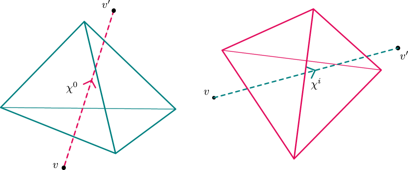
Figure 1: Left: A spacelike tetrahedron (teal) and its corresponding timelike dual edge (pink), connecting the dual vertices $v$ and $v^{\prime}$. Following the restriction in Eq. (25a), the clock $\chi^{0}$ only propagates along timelike dual edges. Right: A timelike tetrahedron (pink) and its corresponding spacelike dual edge (teal). In this case, Eq. (25b) imposes that rods $\chi^{i}$ only propagate along spacelike dual edges.

Given the Lorentzian structure of the original continuum manifold, $\Gamma$ is the dual complex of a Lorentzian discretization. This implies that edges $(vv^{\prime})$ which are dual to spacelike and timelike tetrahedra are timelike and spacelike, respectively, for which a visual intuition is given in Fig. 1. Then, the discrete scalar field action in Eq. (22) can be split into spacelike and timelike dual edges

$$S_{\Gamma}[\chi]=S_{\Gamma}^{+}[\chi]+S_{\Gamma}^{-}[\chi],$$ (23)

defined by

$$S_{\Gamma}[\chi]=\frac{1}{2}\sum_{\mu=0}^{3}\left[\sum_{(vv^{\prime})\text{ t.l.}}w_{vv^{\prime}}(\chi_{v}^{\mu}-\chi_{v^{\prime}}^{\mu})^{2}+\sum_{(vv^{\prime})\text{ s.l.}}w_{vv^{\prime}}(\chi_{v}^{\mu}-\chi_{v^{\prime}}^{\mu})^{2}\right],$$ (24)

where $w_{vv^{\prime}}$ denotes the geometric coefficients $V^{*(4)}_{(vv^{\prime})}/l_{(vv^{\prime})}^{2}$. Clearly, both types of reference fields propagate a priori on both types of dual edges. In analogy to the continuum Equations (21), we propose to align the causal character of the reference frame with that of geometry by introducing the conditions

$$\chi^{0}_{v}-\chi^{0}_{v^{\prime}} =0,\quad\text{for }(vv^{\prime})\text{ spacelike},$$ (25a)

$$\chi^{i}_{v}-\chi^{i}_{v^{\prime}} =0,\quad\text{for }(vv^{\prime})\text{ timelike}.$$ (25b)

Formulated geometrically, the clock propagates along timelike dual edges and rods propagate along spacelike dual edges, as depicted in Fig. 1. As a result, the discrete scalar field action splits into a clock and a rod part, associated to the signature of the respective dual edges. In the following, we discuss the realization of the conditions (25) at the level of the GFT coupling.

Restriction of kinetic kernels.

Proceeding in parallel to Li:2017uao , the scalar field coupling is obtained by considering the simplicial gravity path integral on a given complex $\Gamma$ for the coupled gravity-matter system. As geometric quantities, dual edge lengths and tetrahedron volumes can be re-written in terms of bivector variables $B\in\mathfrak{sl}\left(2,\mathbb{C}\right)$. Then, the GFT model which generates these amplitudes is derived, showing that the details of propagation are encoded in the kinetic kernel, while the GFT interaction is local with respect to the scalar fields. In particular, the details of the discretized geometric quantities $L^{*}_{vv^{\prime}}$ and $V_{vv^{\prime}}^{(3)}$ are encoded in the kinetic kernels, which we keep implicitly defined for the rest of this work.

As a result of the assignment of clocks to timelike dual edges and rods to spacelike dual edges above, the kinetic kernels $\mathcal{K}_{\pm}$ have a restricted dependence, given by

$$\mathcal{K}_{+}({\bf\it g},(\chi-\chi^{\prime})^{2}) =\mathcal{K}_{+}({\bf\it g},(\chi^{0}-\chi^{0\prime})^{2}),$$ (26a)

$$\mathcal{K}_{-}({\bf\it g},(\chi-\chi^{\prime})^{2}) =\mathcal{K}_{-}({\bf\it g},\absolutevalue{{\bf\it\chi}-{\bf\it\chi}^{\prime}}^{2}).$$ (26b)

For the rest of this work, we assume equations (26) to hold (Assumption DS2). Notice again, that the matter field $\phi$ is a priori not affected by this restriction.

3 Coherent peaked states and perturbations

A crucial ingredient for the extraction of cosmological physics is the identification of states that can be associated with continuum, classical physics. Since GFTs are many-body quantum field theories of atoms of spacetime, by analogy with condensed matter systems, one would naturally expect these states to exhibit some form of collective behavior. The simplest form of such collective behavior is captured by coherent (or condensate) states. Importantly, strong evidence has recently been provided for the existence of such a condensate phase in quantum geometric TGFTs Marchetti:2022igl ; Marchetti:2022nrf . One-body condensates of spacelike tetrahedra (whose condensate wavefunction encodes the macroscopic physics of the system) have indeed been used to derive an effective cosmological dynamics that exhibits a resolution of the big bang into a big bounce Oriti:2016qtz ; Marchetti:2020umh ; Jercher:2021bie and offers intriguing phenomenological implications such as dynamical isotropization Pithis:2016cxg , emergent inflation deCesare:2016rsf or a late-time de Sitter phase Oriti:2021rvm . Motivated by these encouraging results and given the need to introduce timelike tetrahedra to improve the frame coupling, we propose to describe the background component of our collective states as the tensor product of a spacelike and a timelike one-body condensate

$$\ket{\sigma;x^{0}}\otimes\ket{\tau;x^{0},{\bf\it x}}=\mathcal{N}_{\sigma}\mathcal{N}_{\tau}\textrm{e}^{\hat{\sigma}\otimes\mathbbm{1}+\mathbbm{1}\otimes\hat{\tau}}\ket{\emptyset},$$ (27)

where the spacelike and timelike condensate states (whose details are discussed in Secs. 3.1.1 and 3.1.2) are denoted as $\ket{\sigma;x^{0}}$ and $\ket{\tau;x^{0},{\bf\it x}}$ respectively. At the right-hand-side of the above equation, we have rewritten the two condensate states as exponentials of the one-body operators $\hat{\sigma}$ and $\hat{\tau}$, respectively acting on the vacuum of $\mathcal{F}_{+}\otimes\mathcal{F}_{-}$. Finally, $\mathcal{N}_{\sigma}$ and $\mathcal{N}_{\tau}$ are normalization factors.

Given the above choice of background states, the most natural way to describe cosmological inhomogeneities would seem to be to include small inhomogeneous perturbations of the one-body condensate wavefunctions (since this is where the macroscopic physics of the system is encoded). However, as it will become clear in Sec. 3.3.1, the mean-field dynamics of the two one-body condensate wavefunctions turn out to be completely decoupled (at least in the regime of negligible interactions that we will consider below). Therefore, this choice would produce results that are effectively equivalent to those found in Marchetti:2021gcv , and thus eventually lead to the puzzling indistinguishably between clocks and rods discussed in the previous section and to the consequent mismatch with GR.

For this reason, and following the intriguing idea that non-trivial geometries are associated with entanglement of quantum gravity degrees of freedom, in this paper we propose an alternative description of cosmological inhomogeneities in terms of correlations of the underlying GFT quanta. Since, however, cosmological inhomogeneities are a macroscopic phenomenon from the QG perspective, the perturbations describing them should be realized in a collective manner at the level of the GFT. Therefore, we consider states of the form

$$\ket{\Delta;x^{0},{\bf\it x}}=\mathcal{N}_{\Delta}\exp(\hat{\sigma}\otimes\mathbbm{1}+\mathbbm{1}\otimes\hat{\tau}+\hat{\delta\Phi}\otimes\mathbbm{1}+\hat{\delta\Psi}+\mathbbm{1}\otimes\hat{\delta\Xi})\ket{\emptyset},$$ (28)

where the small perturbations are encoded in the operators $\hat{\delta\Phi}$, $\hat{\delta\Psi}$ and $\hat{\delta\Xi}$ (see also KS1). In general, these can be a combination of $n$-body operators, each of which encoding $n$-body correlations within and in between the spacelike and timelike sectors. However, in the following, we will restrict to the simplest non-trivial case, i.e. $2$-body operators, whose form is discussed in detail in Sec. 3.2.

Notice that in the picture we propose, we do not consider perturbations at the level of quantum geometric operators but rather at the level of the states, chosen appropriately to describe GR-like perturbations.

Finally, in Sec. 3.3, we derive and discuss the effective relational dynamics of the perturbed states (28).

3.1 Coherent peaked states for spacelike and timelike tetrahedra

As discussed above, our working assumption is that the spacelike and timelike sector of the background structure separate. Since the total Fock space $\mathcal{F}$, introduced in Sec. 2.1, is given in terms of a tensor product of $\mathcal{F}_{+}$ and $\mathcal{F}_{-}$, the states of the background are therefore product states.

3.1.1 Spacelike CPS

On the spacelike Fock space $\mathcal{F}_{+}$, we introduce the coherent peaked state

$$\ket{\sigma_{\epsilon^{+},\pi_{0}^{+}};x^{0}}$$ (29)

$$= \;\mathcal{N}_{\sigma}\exp\left(\int\differential{g_{v}}\differential{X_{+}}\differential[4]{\chi}\differential{\phi}\;\sigma_{\epsilon^{+},\pi_{0}^{+};x^{0}}(g_{v},X_{+},\chi^{0},\phi)\hat{\varphi}^{\dagger}(g_{v},X_{+},\chi^{\mu},\phi)\right)\ket{\emptyset},$$

which is assumed to be normalized via the factor $\mathcal{N}_{\sigma}$ Marchetti:2020umh ; Jercher:2021bie . Key ingredient is the condensate wavefunction $\sigma_{\epsilon^{+},\pi_{0}^{+};x^{0}}$, with $x^{0}$ being the reference field value on which the state is peaked and with $\epsilon^{+}$ and $\pi_{0}^{+}$ characterizing the peaking properties (see Marchetti:2020qsq ; Marchetti:2020umh for further details on the formalism of coherent peaked states). It can be understood as a mean-field, since it is the expectation value of the spacelike group field operator

$$\bra{\sigma_{\epsilon^{+},\pi_{0}^{+}};x^{0}}\hat{\varphi}(g_{v},X_{+},\chi^{\mu},\phi)\ket{\sigma_{\epsilon^{+},\pi_{0}^{+}};x^{0}}=\sigma_{\epsilon^{+},\pi_{0}^{+};x^{0}}(g_{v},X_{+},\chi^{0},\phi).$$ (30)

The condensate wavefunction factorizes as

$$\sigma_{\epsilon^{+},\pi_{0}^{+};x^{0}}(g_{v},X_{+},\chi^{0},\phi)=\eta_{\epsilon^{+}}(\chi^{0}-x^{0};\pi_{0}^{+})\tilde{\sigma}(g_{v},X_{+},\chi^{0},\phi),$$ (31)

wherein

$$\eta_{\epsilon^{+}}(\chi^{0}-x^{0};\pi_{0}^{+})=\mathcal{N}_{\epsilon^{+}}\exp\left(-\frac{(\chi^{0}-x^{0})^{2}}{2\epsilon^{+}}\right)\textrm{e}^{i\pi_{0}^{+}(\chi^{0}-x^{0})}$$ (32)

encodes the Gaussian peaking on the reference field value $x^{0}$ together with a phase factor that ensures finiteness of the reference field momenta Marchetti:2020umh ; Jercher:2021bie (see also KS3). $\mathcal{N}_{\epsilon}^{+}$ is a normalization factor of the Gaussian function. The remaining geometric information is carried by the reduced condensate wavefunction $\tilde{\sigma}(g_{v},X_{+},\chi^{0},\phi)$.

Choice of spacelike peaking.

We have chosen a particular peaking for the spacelike condensate wavefunction as well as a specific dependence on the components of the reference fields $\chi^{\mu}$. Recall that the group field $\varphi(g_{v},X_{+},\chi^{\mu},\phi)$ does depend on all components of the reference fields, even if the kinetic kernel is restricted according to Eq. (26a). However, since we want the background condensates to be associated to perfectly homogeneous geometries, the condensate wavefunction is peaked only on a chosen clock-value and the reduced condensate wavefunction is a function of the clock only (Assumption KS3).

Symmetries of $\tilde{\sigma}$.

Importantly, the reduced condensate wavefunction $\tilde{\sigma}$ satisfies additional symmetries besides that of the group field, given in Eqs. (2) and (3). First, notice that the embedding of a single tetrahedron in Minkowski space, as dictated by the group field, is not a gauge-invariant information. In fact, we argue that the embedding information should be realized in a relational fashion, which is ensured by the clock-peaking. As argued in Jercher:2021bie , so-called adjoint covariance

$$\tilde{\sigma}(g_{v},X_{+},\chi^{0},\phi)=\tilde{\sigma}(hg_{v}h^{-1},h\cdot X_{+},\chi^{0},\phi),\qquad\forall h\in\text{SL$(2,\mathbb{C})$},$$ (33)

can be understood as averaging over the embedding of a single tetrahedron, therefore eliminating this gauge-variant information. The resulting domain of the reduced condensate wavefunction carries the correct number of degrees of freedom, corresponding to the homogeneous spatial metric at a relational instance of time, i.e. it is diffeomorphic to minisuperspace Gielen:2014ila ; Jercher:2021bie ; Marchetti:2020umh . We refer to this property as relational homogeneity Marchetti:2020umh . The remaining two conditions are most clearly seen in spin-representation. A priori, the four spacelike faces of a tetrahedron, labelled by $\rho_{i}$, take different values. Imposing however that the tetrahedra are equilateral, which is often referred to as an isotropy condition Oriti:2016qtz ; Jercher:2021bie , we fix for the remainder all $\rho_{i}$ to be equal (Assumption KS2). Furthermore, the SL$(2,\mathbb{C})$-intertwiner labels arising from Eq. (33) are fixed Jercher:2021bie . To simplify matters even further, we assume that the condensate is dominated by a single spin label $\rho$, as justified by Gielen:2016uft ; Pithis:2016cxg ; Jercher:2021bie (Assumption DC2). As a result of all of these additional conditions, the reduced condensate wavefunction has a spin-representation given by

$$\tilde{\sigma}_{\rho}(\chi^{0},\phi)\equiv\tilde{\sigma}(\chi^{0},\phi),$$ (34)

where we suppress the fixed label $\rho$ in the notation for the remainder. Following this introduction of coherent states for the spacelike background, we elaborate in the following on the timelike background.

3.1.2 Timelike CPS

Following the arguments of the introduction of this section, we assume the timelike background to be described by a condensate which, as it turns out in Sec. 4, proves sufficient to capture GR-like perturbations. Following this idea, we denote the condensate state on $\mathcal{F}_{-}$ as

$$\ket{\tau_{\epsilon^{-},\pi_{0}^{-},\delta,\pi_{x}};x^{0},{\bf\it x}}$$ (35)

$$= \;\mathcal{N}_{\tau}\exp\left(\int\differential{g_{v}}\differential{X_{-}}\differential[4]{\chi}\differential{\phi}\;\tau_{\epsilon^{-},\pi_{0}^{-},\delta,\pi_{x};x^{0},{\bf\it x}}(g_{v},X_{-},\chi^{\mu},\phi)\hat{\varphi}^{\dagger}(g_{v},X_{-},\chi^{\mu},\phi)\right)\ket{\emptyset},$$

which is now an eigenstate of the timelike group field operator, again normalized by the factor $\mathcal{N}_{\tau}$. Similar to the spacelike case, the timelike condensate wavefunction $\tau_{\epsilon^{-},\pi_{0}^{-},\delta,\pi_{x};x^{0},{\bf\it x}}$ factorizes according to

$$\tau_{\epsilon^{-},\pi_{0}^{-},\delta,\pi_{x};x^{0},{\bf\it x}}(g_{v},X_{-},\chi^{\mu},\phi)=\eta_{\epsilon^{-}}(\chi^{0}-x^{0},\pi_{0}^{-})\eta_{\delta}(\absolutevalue{{\bf\it\chi}-{\bf\it x}},\pi_{x})\tilde{\tau}(g_{v},X_{-},\chi^{0},\phi),$$ (36)

where $\tilde{\tau}(g_{v},X_{-},\chi^{0},\phi)$ is the timelike reduced condensate wavefunction. Besides a clock-peaking, the timelike condensate is also peaked on the rod variables ${\bf\it\chi}$ via

$$\eta_{\delta}(\absolutevalue{{\bf\it\chi}-{\bf\it x}},\pi_{x})=\mathcal{N}_{\delta}\exp\left(-\frac{\absolutevalue{{\bf\it\chi}-{\bf\it x}}^{2}}{2\delta}\right)\textrm{e}^{i\pi_{x}\absolutevalue{{\bf\it\chi}-{\bf\it x}}}.$$ (37)

We have chosen an isotropic peaking of the rod variables with the same parameters $\delta$ and $\pi_{x}$ for every spatial direction, following the strategy of Marchetti:2021gcv (see also KS2 and KS3).

Choice of timelike peaking.

Since the timelike condensate is associated to the background structure, the reduced condensate wavefunction $\tilde{\tau}(g_{v},\chi^{0},\phi,X_{-})$ only depends on the relational clock $\chi^{0}$. A peaking on rod variables is added for the timelike condensate to associate spatial derivatives to the timelike sector, as we discuss in more detail in Sec. 3.3.2 (see also Assumption KS3).

Symmetries of $\tilde{\tau}$.

In addition to the symmetries of $\hat{\varphi}(g_{v},X_{-},\chi^{\mu},\phi)$, we introduce additional conditions to the timelike reduced condensate wavefunction $\tilde{\tau}$, similar to $\tilde{\sigma}$ above. Most importantly, these restrictions ensure that $\tilde{\tau}$ carries the correct degrees of freedom. First, $\tilde{\tau}$ also satisfies adjoint covariance

$$\tilde{\tau}(g_{v},X_{-},\chi^{0},\phi)=\tilde{\tau}(hg_{v}h^{-1},h\cdot X_{-},\chi^{0},\phi),\qquad\forall h\in\text{SL$(2,\mathbb{C})$},$$ (38)

with the resulting SL$(2,\mathbb{C})$-intertwiner label in spin-representation being fixed. As a result, the domain of $\tilde{\tau}$ corresponds to the metric degrees of freedom on a $(2+1)$-dimensional slice at a given instance of relational time. Therefore, the number of degrees of freedom of the spacelike and timelike condensates is the same, which is important for the later analysis. Since timelike tetrahedra admit for an arbitrary mixture of spacelike and timelike faces, the reduced condensate wavefunction $\tilde{\tau}$ carries a priori all possible combinations of $(\rho,0)$ and $(0,\nu)$ labels, as Eq. (6) indicates. In the following, we are going to restrict to the case where the condensate wavefunction only carries spacelike faces and fix the corresponding label to the same label $\rho$ as for $\tilde{\sigma}$ (Assumptions KS2, KS4 and DC2). As a result, the timelike reduced condensate wavefunction in spin-representation is of the form

$$\tilde{\tau}_{\rho}(\chi^{0},\phi)\equiv\tilde{\tau}(\chi^{0},\phi),$$ (39)

where we again suppress the fixed label $\rho$ in the remainder.

In summary, the background structure on the total Fock space is defined by the state

$$\ket{\sigma_{\epsilon^{+},\pi_{0}^{+}};x^{0}}\otimes\ket{\tau_{\epsilon^{-},\pi_{0}^{-},\delta,\pi_{x}};x^{0},{\bf\it x}},$$ (40)

on which the group field operators act accordingly. The effective relational dynamics of this background state is computed in Sec. 3.3.1.

3.2 Perturbed coherent peaked states

Following the introduction of this section, inhomogeneities are encoded in the perturbed coherent peaked state of Eq. (28), with the three $2$-body operators $\hat{\delta\Phi}\otimes\mathbbm{1}_{-},\hat{\delta\Psi}$ and $\mathbbm{1}_{+}\otimes\hat{\delta\Xi}$ sourcing a quantum entanglement within and between the spacelike and timelike sectors.

A priori, the kernels $\delta\Phi,\delta\Psi$ and $\delta\Xi$ that define the three operators above are bi-local functions on the respective domains. On both copies of the domain, we impose the same restrictions as for the spacelike and timelike reduced condensate wavefunctions, respectively (see Assumptions KS3, KS4 and DC2). As a result, the spin-representation of the three kernels is explicitly given by

$$\delta\Phi(\chi^{\mu},\phi,\chi^{\prime\mu},\phi^{\prime}),\qquad\delta\Psi(\chi^{\mu},\phi,\chi^{\prime\mu},\phi^{\prime})\qquad\text{and}\qquad\delta\Xi(\chi^{\mu},\phi,\chi^{\prime\mu},\phi^{\prime}),$$ (41)

where we suppressed the dependence on the fixed SL$(2,\mathbb{C})$-representation label $\rho$ in the notation. Crucially, the three two-body operators do not factorize into one-body operators if the kernels do not factorize accordingly. As a result, acting with $\hat{\delta\Phi},\hat{\delta\Psi}$ and $\hat{\delta\Xi}$ on the tensor product of spacelike and timelike condensate creates an entangled state in the respective sectors.

Finally, $\ket{\Delta;x^{0},{\bf\it x}}$ is the state that we are going to employ for computing the cosmological dynamics, including perturbations. In the following two sections, we show how to obtain effective relational dynamics as the expectation value of the GFT equations of motion and how to connect macroscopic quantities such as the $3$-volume to the expectation value of quantum geometric operators.

3.3 Effective relational dynamics of perturbed CPS

Average relational dynamics of GFT condensates are, at a mean-field level, obtained by taking the expectation value of the GFT equations of motion with respect to the macroscopic state $\ket{\Delta;x^{0},{\bf\it x}}$, see also DS3. Due to the presence of two fields, corresponding to spacelike and timelike tetrahedra, there are two effective relational equations of motion, which are given by

$$\expectationvalue{\functionalderivative{S[\hat{\varphi},\hat{\varphi}^{\dagger}]}{\hat{\varphi}(g_{v},X_{\alpha},x^{\mu},\phi)}}{\Delta;x^{0},{\bf\it x}}=0,$$ (42)

for each signature $\alpha\in\{+,-\}$. Notice, that these equations correspond to the first of an infinite tower of Schwinger-Dyson equations Oriti:2016qtz ; Gielen:2013naa .

For the remainder of this work, we assume negligible interactions (Assumption DS4), which was shown in Oriti:2016qtz ; Jercher:2021bie to be a valid approximation at late but not very late times, see also Gielen:2013naa for a discussion. Notice, that the argument provided therein also applies to the timelike sector. One of the crucial consequences of this assumption is that higher orders of the Schwinger-Dyson equations reduce to powers of the lowest order equations (42), as we show in Appendix B. Hence, solutions of Eq. (42) solve also all higher orders. We comment on this matter in more detail in Sec. 5. Notice that despite negligible interactions, the spacelike and timelike sectors get coupled via the spacelike-timelike quantum correlation $\delta\Psi$, as we show in detail in Sec. 3.3.2.

Due to the presence of perturbations, the two equations of motion can be separated into a zeroth-order background part and a first-order perturbation part, which we discuss separately in Secs. 3.3.1 and 3.3.2, respectively.

3.3.1 Background equations of motion

At background level, the two equations of motion in spin-representation are given by

$$0 =\int\differential{\chi^{0}}\differential{\phi^{\prime}}\mathcal{K}_{+}\left(\chi^{0},(\phi-\phi^{\prime})^{2}\right)\sigma(\chi^{0}+x^{0},\phi^{\prime}),$$ (43)

$$0 =\int\differential[4]{\chi}\differential{\phi^{\prime}}\mathcal{K}_{-}\left({\bf\it\chi},(\phi-\phi^{\prime})^{2}\right)\tau(\chi^{0}+x^{0},{\bf\it\chi}+{\bf\it x},\phi^{\prime}).$$ (44)

For a further analysis, we perform a Fourier transform of the matter field variables $\phi\rightarrow\pi_{\phi}$. Following Marchetti:2021gcv , we assume a peaking of both condensate wavefunctions on a fixed scalar field momentum $p_{\phi}$, realized by a Gaussian peaking. Since the scalar field is minimally coupled, its canonical conjugate momentum is constant at the classical continuum level. We translate this idea to the present context by peaking on a fixed value $p_{\phi}$ (Assumption KC1). Exploiting furthermore the peaking properties of $\sigma$ and $\tau$, defined in Eqs. (31) and (36), respectively, we obtain the dynamical equations for the reduced condensate wavefunctions $\tilde{\sigma}$ and $\tilde{\tau}$

$$\partial_{0}^{2}\tilde{\sigma}(x^{0},p_{\phi})-2i\tilde{\pi}_{0}^{+}\partial_{0}\tilde{\sigma}(x^{0},p_{\phi})-E_{+}^{2}(\pi_{\phi})\tilde{\sigma}(x^{0},p_{\phi}) =0,$$ (45)

$$\partial_{0}^{2}\tilde{\tau}(x^{0},p_{\phi})-2i\tilde{\pi}_{0}^{-}\partial_{0}\tilde{\tau}(x^{0},p_{\phi})-E_{-}^{2}\tilde{\tau}(x^{0},p_{\phi}) =0,$$ (46)

where the quantities $E_{\pm}$ and $\tilde{\pi}_{0}^{\pm}$ are defined in Appendix D.1, to which we refer for further details.

Following the procedure of Oriti:2016qtz ; Marchetti:2020umh ; Marchetti:2021gcv , the reduced condensate wavefunctions can be decomposed into a radial and angular part, denoted as $r_{\alpha}(x^{0},p_{\phi})$ and $\theta_{\alpha}(x^{0},p_{\phi})$, respectively. Splitting the resulting equations into real and imaginary part, one obtains

$$r^{\prime\prime}_{\alpha}(x^{0},p_{\phi})-\frac{Q_{\alpha}^{2}(p_{\phi})}{r_{\alpha}^{3}(x^{0},p_{\phi})}-\mu_{\alpha}^{2}(p_{\phi})r_{\alpha}(x^{0},p_{\phi}) =0,$$ (47)

$$\theta_{\alpha}^{\prime}(x^{0},p_{\phi})-\tilde{\pi}_{0}^{\alpha}-\frac{Q_{\alpha}(p_{\phi})}{r_{\alpha}^{2}(x^{0},p_{\phi})} =0,$$ (48)

where a prime denotes differentiation with respect to $x^{0}$, $Q_{\alpha}$ are integration constants and the $\mu_{\alpha}$ are defined as $\mu_{\alpha}^{2}(p_{\phi})\vcentcolon=E_{\alpha}^{2}(p_{\phi})-(\tilde{\pi}_{0}^{\alpha})^{2}$. As demonstrated in Appendix D.1, $E_{-}$ and thus $\mu_{-}$ are actually independent of the peaked matter momentum $p_{\phi}$.

Classical limit.

As elaborated previously Oriti:2016qtz ; Marchetti:2020umh ; Marchetti:2020qsq , the semi-classical limit of the condensate is obtained at late relational time scales where the moduli of the condensate wavefunctions $r_{\alpha}$ are dominant with respect to $Q_{\alpha}$ and $\mu_{\alpha}$ but where interactions are still negligible (see also DC1). Furthermore, it has been shown in Pithis:2016cxg , that in this limit, expectation values of for instance the volume operator are sharply peaked, providing a highly non-trivial consistency check for the semi-classical interpretation. In this limit, the background equations of motion simplify significantly, yielding solutions

$$\tilde{\sigma}(x^{0},p_{\phi}) =\tilde{\sigma}_{0}\textrm{e}^{(\mu_{+}+i\tilde{\pi}_{0}^{+})x^{0}},$$ (49)

$$\tilde{\tau}(x^{0},p_{\phi}) =\tilde{\tau}_{0}\textrm{e}^{(\mu_{-}+i\tilde{\pi}_{0}^{-})x^{0}},$$ (50)

where $\tilde{\sigma}_{0}$ and $\tilde{\tau}_{0}$ are determined by initial conditions.

This concludes the effective background equations of motion. In the next section, we compute the effective equations of motion at first order in perturbations.

3.3.2 Perturbed equations of motion

At first order in perturbations, there are two equations, one for the spacelike and one for the timelike sector. Since there are three distinct two-body correlations $\delta\Phi,\delta\Psi$ and $\delta\Xi$, there is a dynamical freedom for one of the variables if one assumes negligible interactions and works within a first-order perturbative framework. In the following, we utilize this freedom to relate the functions $\delta\Phi$ and $\delta\Psi$ via an arbitrary function $\mathrm{f}(\chi^{\mu})$ that will be ultimately fixed by matching the perturbed volume to the classical quantity of GR. We provide a physical interpretation of this assumption in Sec. 4.2 in terms of the perturbations of the timelike number operator, $\delta N_{-}$.

Spacelike perturbed dynamics.

Dynamics of the spacelike sector at first order of perturbations are governed by

$$0 =\int\differential[4]{\chi}\differential{\phi^{\prime}}\mathcal{K}_{+}((\chi^{0})^{2},(\phi-\phi^{\prime})^{2})\int\differential[4]{\chi^{\prime}}\differential{\phi^{\prime\prime}}\Bigg{[}\delta\Psi(\chi^{\mu}+x^{\mu},\phi^{\prime},\chi^{\mu\prime},\phi^{\prime\prime})\bar{\tau}(\chi^{\mu\prime},\phi^{\prime\prime})$$ (51)

$$+\delta\Phi(\chi^{\mu}+x^{\mu},\phi^{\prime},\chi^{\mu\prime},\phi^{\prime\prime})\bar{\sigma}(\chi^{0\prime},\phi^{\prime\prime})\Bigg{]}.$$

As a first simplification, we choose the bi-local kernel $\delta\Psi$ to depend only on one copy of relational frame data (Assumption KC2), i.e.

$$\delta\Psi(\chi^{\mu},\pi_{\phi},\chi^{\mu\prime},\pi_{\phi}^{\prime}) =\delta\Psi(\chi^{\mu},\pi_{\phi})\delta^{(4)}(\chi^{\mu}-\chi^{\prime\mu})\delta(\pi_{\phi}-\pi_{\phi}^{\prime}).$$ (52)

From a simplicial gravity perspective, locality with respect to the reference fields $\chi^{\mu}$ corresponds to correlations only within the same $4$-simplex, which can be compared to nearest-neighbor interactions in statistical spin systems. For the momenta of the matter field $\pi_{\phi}$, the condition is interpreted as momentum conservation across tetrahedra of the same $4$-simplex. Next, we exploit the dynamical freedom for one of the perturbation functions by imposing the relation (Assumption DC3)

$$\delta\Phi(\chi^{\mu},\pi_{\phi})=\mathrm{f}(\chi^{\mu})\delta\Psi(\chi^{\mu},\pi_{\phi}),$$ (53)

with the complex valued function $\mathrm{f}$ defined as

$$\mathrm{f}(\chi^{0},{\bf\it\chi})=f(\chi^{0})\textrm{e}^{i\theta_{f}(\chi^{0})}\absolutevalue{\eta_{\delta}(\absolutevalue{{\bf\it\chi}-{\bf\it x}})}\textrm{e}^{2i\pi_{0}^{+}\chi^{0}}.$$ (54)

Here, $f$ and $\theta_{f}$ are real functions that only depend on the reference clock $\chi^{0}$. In addition, we consider the following relations between the peaking parameters $\epsilon^{\pm}$ and $\pi_{0}^{\pm}$ of the different sectors

$$\epsilon^{+}=\epsilon^{-},\qquad\pi_{0}^{+}=-\pi_{0}^{-},$$ (55)

also entering Assumption KC3. Besides simplifying the spacelike equations of motion at first order in perturbations, we show in Sec. 4.1 that the expression of the perturbed $3$-volume $\delta V$ takes a manageable form under Eq. (55).

Within this set of choices, the peaking properties of the spacelike and timelike condensate wavefunctions yield the following equation of motion for $\delta\Psi$

$$0 =\partial_{0}^{2}\left(\delta\Psi(J_{0}\bar{\tilde{\tau}}+f\textrm{e}^{i\theta_{f}}\bar{\tilde{\sigma}})\right)-2i\tilde{\pi}_{0}^{+}\partial_{0}\left(\delta\Psi(J_{0}\bar{\tilde{\tau}}+f\textrm{e}^{i\theta_{f}}\bar{\tilde{\sigma}})\right)+$$ (56)

$$-E_{+}^{2}\delta\Psi(J_{0}\bar{\tilde{\tau}}+f\textrm{e}^{i\theta_{f}}\bar{\tilde{\sigma}})+\alpha\bar{\tilde{\tau}}\nabla_{{\bf\it x}}^{2}\delta\Psi,$$

for which a detailed derivation is provided in Appendix D.2. All of the functions above depend on the peaked value of the matter momentum, $p_{\phi}$, but we suppress that dependence for notational clarity. As written out explicitly before, the two reduced condensate wavefunctions $\tilde{\sigma}$ and $\tilde{\tau}$ depend on the relational time $x^{0}$ since they are part of the background, while in contrast, $\delta\Psi(x^{\mu},p_{\phi})$ depends on all four reference field values. The remaining coefficients $E_{+}(p_{\phi}),\tilde{\pi}_{0}^{+},J_{0}$ and $\alpha$ are defined in Appendix D.2 and are entirely determined by peaking parameters and the peaked matter momentum $p_{\phi}$.

Solving the background equations of motion and inserting them in the first-order perturbation equation, one obtains an equation for $\delta\Psi$ which is of the general form

$$0=\delta\Psi^{\prime\prime}+t_{1}(x^{0},p_{\phi})\delta\Psi^{\prime}+t_{0}(x^{0},p_{\phi})\delta\Psi+s_{2}(x^{0},p_{\phi})\nabla_{{\bf\it x}}^{2}\delta\Psi,$$ (57)

with complex coefficients functions $t_{i}(x^{0},p_{\phi})$ and $s_{2}(x^{0},p_{\phi})$. The conditions on these coefficients to yield GR-like perturbation equations are discussed in Sec. 4.

Timelike perturbed dynamics.

As we will explicitly see in the next section, the dynamics of observables other than the spatial $3$-volume, such as the matter field, its momentum or the total number operator, are governed by the equations of motion of both sectors, spacelike and timelike. For this reason, in the following, we study the perturbed equations of motion on the timelike sector which, in spin-representation, are given by

$$0 =\int\differential[4]{\chi}\differential{\phi^{\prime}}\mathcal{K}_{-}(\absolutevalue{{\bf\it\chi}}^{2},(\phi-\phi^{\prime})^{2})\int\differential[4]{\chi^{\prime}}\differential{\phi^{\prime\prime}}\Bigg{[}\delta\Psi(\chi^{0\prime},{\bf\it\chi}^{\prime},\phi^{\prime},\chi^{\mu}+x^{\mu},\phi^{\prime\prime})\bar{\sigma}(\chi^{0\prime},\phi^{\prime\prime})$$ (58)

$$+\delta\Xi(\chi^{\mu}+x^{\mu},\phi^{\prime},\chi^{0\prime},{\bf\it\chi}^{\prime},\phi^{\prime\prime})\bar{\tau}(\chi^{\mu\prime},\phi^{\prime\prime})\Bigg{]}.$$

Using the peaking properties of $\sigma$ and $\tau$, the locality condition in Eq. (52), the relation of peaking parameters in Eq. (55), as well as the classical background equations of motion in Eqs. (49) and (50), one obtains

$$0 =\bar{\tilde{\sigma}}\int\differential[3]{\chi}\mathcal{K}_{-}(\absolutevalue{{\bf\it\chi}},p_{\phi}^{2})\left[\partial_{0}^{2}\delta\Psi+2\mu_{+}\partial_{0}\delta\Psi-\frac{\mathcal{K}_{+}^{(2)}}{\mathcal{K}_{+}^{(0)}}\delta\Psi\right]$$ (59)

$$+\bar{\tilde{\tau}}\mathcal{K}_{-}^{(0)}J_{0,{\bf\it 0}}\Bigg{[}\partial_{0}^{2}\delta\Xi+2\mu_{-}\partial_{0}\delta\Xi-\beta\delta\Xi+\gamma\nabla_{{\bf\it x}}^{2}\delta\Xi\Bigg{]},$$

for which a derivation is given in Appendix D.2, including a definition of the parameters $\beta$ and $\gamma$. Since the space-dependence of the first term is integrated out, solutions $\delta\Xi$ need to be space-independent, i.e. $\delta\Xi(x^{\mu},p_{\phi})\equiv\delta\Xi(x^{0},p_{\phi})$. Hence, the space-derivative acting on $\delta\Xi$ vanishes and the equation reduces to a second-order inhomogeneous ordinary differential equation. In particular, the pure time dependence of $\delta\Xi$ will have important consequences for the behavior of timelike particle number perturbations $\delta N_{-}$, discussed in detail in Sec. 4.2.

4 Dynamics of observables

In the spirit of obtaining cosmology as a hydrodynamic limit of QG, classical cosmological quantities are associated with averages on the above condensate states of appropriate one-body observables defined within the GFT Fock space. Importantly, this can only hold under the assumption that quantum fluctuations of such observables on the states of interest are small. As emphasized in Marchetti:2020qsq ; Gielen:2019kae , this classicality requirement is automatically satisfied at late relational times. For this reason, in the following we will focus only on this regime.

Observables of interest for cosmological applications can be roughly divided into two categories: geometric observables (such as volume, area, curvature, etc.) and matter observables (such as the scalar field operators and their momenta). However, as one might expect, not all operators available in the quantum theory fall into these two categories. A particularly important example of “observables” that have no classical counterpart are number operators, i.e. operators that count the number of GFT (timelike and/or spacelike) quanta. In fact, the classical limit turns out to be associated with a large number of quanta in the condensate and is thus directly controlled by the above quantities.

In the following, we will compute expectation values of geometric, number, and matter operators in Sec. 4.1$-$4.3, respectively. In the geometric sector we will restrict ourselves to the expectation value of the volume operator. Note that while this is clearly sufficient to characterize the full geometry of a homogeneous and isotropic universe, it is a strong restriction at the perturbation level, since it can only capture scalar, isotropic inhomogeneities. To extract a full-fledged cosmological perturbation theory from GFTs, it is therefore imperative to construct more sophisticated geometric observables. This is an avenue of research that has been only tentatively explored Gielen:2021vdd ; Calcinari:2022iss . We will return to this topic in Sec. 5.

More concretely, one can compute the expectation value of a second-quantized operator $\hat{\mathcal{O}}$ on the perturbed condensate states $\ket{\Delta;x^{0},{\bf\it x}}$ by using the algebra of creation and annihilation operators. The result can be split generically as

$$\mathcal{O}(x^{0},{\bf\it x})\equiv\expectationvalue{\hat{\mathcal{O}}}{\Delta;x^{0},{\bf\it x}}=\bar{\mathcal{O}}(x^{0})+\delta\mathcal{O}(x^{0},{\bf\it x}),$$ (60)

where $\bar{\mathcal{O}}$ and $\delta\mathcal{O}$ are background and perturbed contributions, respectively. Note that, due to the peaking properties of the states $\ket{\Delta;x^{0},{\bf\it x}}$, the above expectation value is localized in relational space and time. In this sense, the quantities obtained are effective relational observables. As such, their dynamics should be compared, at least in an appropriate limit, with the dynamics of the corresponding classical cosmological relational observables. Since these are gauge-invariant extensions of gauge-fixed quantities, one could alternatively compare the dynamics of the above expectation values with the dynamics of the corresponding classical cosmological observables in harmonic gauge (since the physical frame used to localize quantities is in fact harmonic) Gielen:2013naa ; Oriti:2016qtz ; Marchetti:2020umh ; Marchetti:2021gcv , as derived in Appendix C. This will be the goal of Sec. 4.5.

4.1 Volume operator and related geometric observables

An operator that captures the isotropic information of the spatial geometry is the $3$-volume operator defined in Eq. (14). We study its expectation value with respect to the perturbed condensate state in this section.

Using the choices on the perturbation functions $\delta\Phi$ and $\delta\Psi$ in Eqs. (52) and (53), respectively, the expectation value of $\hat{V}$ is given by

$$\expectationvalue{\hat{V}}{\Delta;x^{0},{\bf\it x}} =v\int\differential[4]{\chi}\differential{\pi_{\phi}}\bar{\sigma}(\chi^{0},\pi_{\phi})\sigma(\chi^{0},\pi_{\phi})$$ (61)

$$\quad+2v\mathfrak{Re}\left\{\int\differential[4]{\chi}\differential{\pi_{\phi}}\delta\Psi(\chi^{\mu},\pi_{\phi})\bar{\sigma}(\chi^{0},\pi_{\phi})\bar{\tau}(\chi^{\mu},\pi_{\phi})\right\}$$

$$\quad+2v\mathfrak{Re}\left\{\int\differential[4]{\chi}\differential{\pi_{\phi}}\mathrm{f}(\chi^{\mu})\delta\Psi(\chi^{\mu},\pi_{\phi})\bar{\sigma}(\chi^{0},\pi_{\phi})\bar{\sigma}(\chi^{0},\pi_{\phi})\right\},$$

where $v$ is similar to a volume eigenvalue Oriti:2016qtz ; Jercher:2021bie , scaling as $\rho^{3/2}$. Applying Eq. (55) and exploiting the peaking properties of $\sigma$ and $\tau$, the volume expectation value becomes

$$\expectationvalue{\hat{V}}{\Delta;x^{0},{\bf\it x}}=v\absolutevalue{\tilde{\sigma}(x^{0},p_{\phi})}^{2}\int\differential[3]{\chi}$$ (62)

$$\quad+2v\mathfrak{Re}\left\{J_{0}\delta\Psi(x^{\mu},p_{\phi})\bar{\tilde{\sigma}}(x^{0},p_{\phi})\bar{\tilde{\tau}}(x^{0},p_{\phi})+\frac{J_{2}}{2}\bar{\tilde{\sigma}}(x^{0},p_{\phi})\bar{\tilde{\tau}}(x^{0},p_{\phi})\nabla_{{\bf\it x}}^{2}\delta\Psi(x^{\mu},p_{\phi})\right\}$$

$$\quad+2v\mathfrak{Re}\left\{\delta\Psi(x^{\mu},p_{\phi})f(x^{0})\textrm{e}^{i\theta_{f}(x^{0})}\bar{\tilde{\sigma}}(x^{0},p_{\phi})\bar{\tilde{\sigma}}(x^{0},p_{\phi})\right\}.$$

The first term, containing an empty rod-integration (see Assumption KS5), defines the background volume

$$\bar{V}=v\absolutevalue{\tilde{\sigma}(x^{0},p_{\phi})}^{2},$$ (63)

while the remaining two contributions make up the perturbations of the volume

$$\delta V(x^{\mu},p_{\phi})=2v\mathfrak{Re}\left\{\delta\Psi(x^{\mu},p_{\phi})f(x^{0})\textrm{e}^{i\theta_{f}(x^{0})}\bar{\tilde{\sigma}}(x^{0},p_{\phi})\bar{\tilde{\sigma}}(x^{0},p_{\phi})\right\}$$ (64)

$$\quad+2v\mathfrak{Re}\left\{J_{0}\delta\Psi(x^{\mu},p_{\phi})\bar{\tilde{\sigma}}(x^{0},p_{\phi})\bar{\tilde{\tau}}(x^{0},p_{\phi})+\frac{J_{2}}{2}\bar{\tilde{\sigma}}(x^{0},p_{\phi})\bar{\tilde{\tau}}(x^{0},p_{\phi})\nabla_{{\bf\it x}}^{2}\delta\Psi(x^{\mu},p_{\phi})\right\}.$$

From the dynamics derived in Sec. 3.3, we can straightforwardly obtain the dynamics of the background and the perturbed averaged volume. This will be done in the next two paragraphs.

Background volume.

At the level of the background, the expectation value of the spatial volume operator in a classical limit (see Assumption DC1) is given by

$$\bar{V}(x^{0},p_{\phi})=\tilde{\sigma}_{0}^{2}\textrm{e}^{2\mu_{+}x^{0}}.$$ (65)

Performing derivatives with respect to the clock field value $x^{0}$, $\bar{V}$ satisfies

$$\frac{\bar{V}^{\prime}}{3\bar{V}}=\frac{2}{3}\mu_{+}(p_{\phi}),\qquad\left(\frac{\bar{V}^{\prime}}{3\bar{V}}\right)^{\prime}=0.$$ (66)

Defining the quantity $\mathcal{H}=\bar{V}^{\prime}/(3\bar{V})$, these equations can be recast as

$$\mathcal{H}^{2}=\frac{4}{9}\mu_{+}^{2}(p_{\phi}),\qquad\mathcal{H}^{\prime}=0.$$ (67)

Comparing with the classical background equations from general relativity in units where $8\pi G=1$, summarized in Sec. C.1, matching with the GFT dynamics is found if

$$\mu_{+}^{2}(p_{\phi})=\frac{3}{8M_{\mathrm{Pl}}^{2}}\bar{\pi}_{\phi}^{2},$$ (68)

where $\bar{\pi}_{\phi}$ is the constant momentum of the matter field $\phi$ at background level. The factor of the Planck mass is present at the level of the classical Einstein equations (see Eq. (152)) and thus needs to be accounted for in the matching procedure. Working with fields of energy dimension $1$, $[\phi]=1$, and thus with conjugate momenta of energy dimension $2$, $[\pi_{\phi}]=2$, the matching is therefore consistent with the fact that $[\mu_{+}]$ is required to be $1$.

Volume perturbations.

To study the dynamics of $\delta V$ (defined in Eq. (LABEL:eq:pert_volume_expval)) it is convenient to perform a split of the complex-valued function $\delta\Psi$ into its modulus and phase, $\delta\Psi=R(x^{\mu},p_{\phi})\textrm{e}^{i\Theta}$. We pose the condition that this phase is in fact constant, see also Assumption DC4. As a result, the overall phases of the first and second term inside the real parts of $\delta V$ are respectively given by

$$\theta_{1} =\Theta+\theta_{f}(x^{0})-2\tilde{\pi}_{0}^{+}x^{0},$$ (69)

$$\theta_{2} =\Theta.$$ (70)

Exploiting once more the dynamical freedom on $\delta\Phi$, and thus on the function $\mathrm{f}(\chi^{0},{\bf\it\chi})$ entering Eq. (53), we set $\theta_{f}=\frac{\pi}{2}+2\tilde{\pi}_{0}^{+}x^{0}$. In momentum space of the rod variable, which we consider for the remainder of Section 4, the resulting form of $\delta V$ is given by

$$\frac{\delta V(x^{0},k)}{2v\tilde{\sigma}_{0}\tilde{\tau}_{0}}=\left[\cos(\Theta)\textrm{e}^{(\mu_{+}+\mu_{-})x^{0}}\left(J_{0}-\frac{J_{2}}{2}k^{2}\right)+\sin(\Theta)\textrm{e}^{2\mu_{+}x^{0}}\frac{\tilde{\sigma}_{0}}{\tilde{\tau}_{0}}f\right]R.$$ (71)

Put in this form, the perturbed volume $\delta V$ is directly related to the modulus $R$ by a time- and momentum-dependent factor $A$,

$$\frac{\delta V(x^{0},k)}{2v\tilde{\sigma}_{0}\tilde{\tau}_{0}}=\vcentcolon A(x^{0},k)R.$$ (72)

Therefore, the dynamics of $\delta V$ are essentially governed by the dynamics of $R$, which we discuss next.

Introducing the function

$$g_{f}\vcentcolon=\left(\tilde{\sigma}_{0}f\textrm{e}^{\mu_{+}x^{0}}+J_{0}\tilde{\tau}_{0}\textrm{e}^{\mu_{-}x^{0}}\right),$$ (73)

the dynamics of $\delta\Psi=R\textrm{e}^{i\Theta}$ for a constant phase $\Theta$ are given by

$$0=R^{\prime\prime}+2\frac{g_{f}^{\prime}}{g_{f}}R^{\prime}+\left(\frac{g_{f}^{\prime\prime}}{g_{f}}-\mu_{+}^{2}\right)R-\frac{\alpha\tilde{\tau}_{0}\textrm{e}^{\mu_{-}x^{0}}}{g_{f}}k^{2}R\,,$$ (74)

which straightforwardly follows from Eq. (56) and the derivations of Sec. 3.3.2. Combining Eqs. (71) and (74), the dynamical equation for the perturbed volume $\delta V$ is given by

$$\delta V^{\prime\prime}+\left[2\frac{g_{f}^{\prime}}{g_{f}}-2\frac{A^{\prime}}{A}\right]\delta V^{\prime}+\left[\frac{g_{f}^{\prime\prime}}{g_{f}}-\mu_{+}^{2}+2\left(\frac{A^{\prime}}{A}\right)^{2}-\frac{A^{\prime\prime}}{A}-2\frac{g_{f}^{\prime}}{g_{f}}\frac{A^{\prime}}{A}\right]\delta V-\frac{\alpha\tilde{\tau}_{0}\textrm{e}^{\mu_{-}x^{0}}}{g_{f}}k^{2}\delta V=0\,.$$ (75)

The above equation, and thus any solution of it, clearly depends on the function $g_{f}$ encoding the aforementioned mean-field dynamical freedom. Remarkably, however, this freedom can be fixed entirely by requiring the above equation to take the same functional form (at least in the late time, classical regime) of the corresponding GR one, given in Eq. (167).

To see this explicitly, we start from the spatial derivative term, whose pre-factor $a^{4}$, as mentioned in Sec. 1, could not be recovered by considering a perturbed condensate of only spacelike tetrahedra Marchetti:2021gcv . Exactly because of the additional timelike degrees of freedom, and thus of the above dynamical freedom, here we can easily recover the appropriate pre-factor, by simply requiring the function $g_{f}$ to satisfy

$$-\frac{\alpha\tilde{\tau}_{0}\textrm{e}^{\mu_{-}x^{0}}}{g_{f}}=a^{4}=\tilde{\sigma}_{0}^{8/3}\textrm{e}^{8\mu_{+}x^{0}/3},$$ (76)

where $a$ is the scale factor. The above condition corresponds to the following choice of $f$:

$$f=-\frac{\tilde{\tau}_{0}}{\tilde{\sigma}_{0}}\textrm{e}^{(\mu_{-}-\mu_{+})x^{0}}\left(J_{0}+\alpha a^{-4}\right),$$ (77)

fixing the aforementioned dynamical freedom completely (see Assumption DC3).

As a result of this fixing, the function $g_{f}$ satisfies the following derivative properties

$$\frac{g_{f}^{\prime}}{g_{f}}=\mu_{-}-\frac{8}{3}\mu_{+},\qquad\frac{g_{f}^{\prime\prime}}{g_{f}}=\left(\mu_{-}-\frac{8}{3}\mu_{+}\right)^{2}.$$ (78)

Inserting the expression of $f$ into the function $A(x^{0},k)$, one obtains

$$\frac{A^{\prime}}{A}=\mu_{+}+\mu_{-}+\frac{8}{3}\mu_{+}\frac{\alpha\frac{\tilde{\tau}_{0}}{\tilde{\sigma}_{0}}\sin(\Theta)a^{-4}}{\cos(\Theta)\left(J_{0}-\frac{J_{2}}{2}k^{2}\right)-\frac{\tilde{\tau}_{0}}{\tilde{\sigma}_{0}}\sin(\Theta)\left(J_{0}+\alpha a^{-4}\right)}.$$ (79)

As we see from the above equation, in general $A$ is a complicated function of the momenta $k$. As a consequence, the same holds for the factors in front of $\delta V^{\prime}$ and $\delta V$ in Eq. (75). This is in sharp contrast to what happens in GR, see again Eq. (167). However, this undesired $k$-dependence can be easily removed by choosing $\Theta=n\frac{\pi}{2}$ with odd integer $n$ and assuming that $J_{0}$ is negligible with respect to $\alpha a^{-4}$ (Assumptions KC3, DC4 and DC5). Under these assumptions, the derivatives of $A$ take the form

$$\frac{A^{\prime}}{A}=-\frac{5}{3}\mu_{+}+\mu_{-},\qquad\frac{A^{\prime\prime}}{A}=\left(-\frac{5}{3}\mu_{+}+\mu_{-}\right)^{2}.$$ (80)

Combining Eqs. (78) and (80), the perturbed volume equation attains the form

$$\delta V^{\prime\prime}-3\mathcal{H}\delta V^{\prime}+a^{4}k^{2}\delta V=0,$$ (81)

where we identified $\mathcal{H}=\frac{2}{3}\mu_{+}$ from the background equations. Expressed instead in terms of the ratio $\delta V/\bar{V}$, the relative perturbed volume equation is given by

$$\left(\frac{\delta V}{\bar{V}}\right)^{\prime\prime}+3\mathcal{H}\left(\frac{\delta V}{\bar{V}}\right)^{\prime}+a^{4}k^{2}\left(\frac{\delta V}{\bar{V}}\right)=0.$$ (82)

Remarkably, the two coefficients in front of the zeroth and first derivative term in Eq. (81) are both completely fixed by the background parameter $\mu_{+}$. In fact, the parameter $\mu_{-}$, characterizing the behavior of the timelike condensate, does not enter the perturbed volume equation at all. Even though the inclusion of a timelike condensate allows to nicely match the functional form of Eq. (82) (in particular solving all the issues reported in Marchetti:2021gcv ) with that of the GR Eq. (125), the GFT volume perturbation equation does show some new intriguing features, which we investigate in detail in Sec. 4.5.

Scale factor observables.

Before closing this section, we would like to emphasize that the cosmological equations obtained at the level of background and perturbations do not depend on the fact that we choose the $3$-volume to encode the (scalar, isotropic) geometric information. In fact, due to homogeneity and isotropy at the level of the background condensate, one could heuristically consider some geometric observable $\mathcal{O}$ whose expectation value is associated to $\absolutevalue{\tilde{\sigma}}^{2}$ at the background level and which would classically be interpreted as an appropriate power of the scale factor: $\left\langle\mathcal{O}\right\rangle\sim a^{d}$. Examples other than the volume would be length for $d=1$ or area for $d=2$. Re-iterating the same derivation as above but now with general $d$, the relation of $\mu_{+}$ and $\mathcal{H}$ is given by

$$\mathcal{H}=\frac{\mathcal{O}^{\prime}}{\mathcal{O}d}=\frac{2\mu_{+}}{d}.$$ (83)

At the perturbed level, the GFT equations would show exactly the same behavior as for the volume, namely

$$\delta\mathcal{O}_{\mathrm{GFT}}^{\prime\prime}-d\mathcal{H}\delta\mathcal{O}_{\mathrm{GFT}}^{\prime}+a^{4}k^{2}\delta\mathcal{O}_{\mathrm{GFT}}=0.$$ (84)

Perturbations of the classical quantity, $\delta\mathcal{O}_{\mathrm{GR}},$ would instead be described by

$$\delta\mathcal{O}_{\mathrm{GR}}^{\prime\prime}-2d\mathcal{H}\delta\mathcal{O}_{\mathrm{GR}}^{\prime}+d^{2}\mathcal{H}^{2}\delta\mathcal{O}_{\mathrm{GR}}+a^{4}k^{2}\delta\mathcal{O}_{\mathrm{GR}}=0\,,$$ (85)

which shows that the differences in the equations of $\delta V$ from GFT and GR do not arise from considering the “wrong” geometric observable.

4.2 Number of quanta

The number operator, introduced in Eq. (13), is clearly the simplest second-quantized operator available in the Fock space. However, as we mentioned above, it is extremely important to characterize the classical and continuum limit of the QG system. On the two-sector Fock space, one can define individual number operators $\hat{N}_{\alpha}$, counting the number of spacelike and timelike tetrahedra, respectively, or the total number operator $\hat{N}=\hat{N}_{+}+\hat{N}_{-}$. Forming the expectation value of $\hat{N}_{\alpha}$ with respect to $\ket{\Delta;x^{0},{\bf\it x}}$, the contributions of the background and perturbations are respectively given by

$$\bar{N}_{+} =\absolutevalue{\tilde{\sigma}(x^{0},p_{\phi})}^{2},$$ (86)

$$\bar{N}_{-} =\absolutevalue{\tilde{\tau}(x^{0},p_{\phi})}^{2},$$ (87)

and

$$\delta N_{+} =2\mathfrak{Re}\left\{\int\differential[4]{\chi}\differential{\pi_{\phi}}\delta\Psi(\chi^{\mu},\pi_{\phi})\left[\bar{\sigma}(\chi^{0},\pi_{\phi})\bar{\tau}(\chi^{\mu},\pi_{\phi})+\mathrm{f}(\chi^{\mu})\bar{\sigma}^{2}(\chi^{0},\pi_{\phi})\right]\right\},$$ (88)

$$\delta N_{-} =2\mathfrak{Re}\left\{\int\differential[4]{\chi}\differential{\pi_{\phi}}\left[\delta\Psi(\chi^{\mu},\pi_{\phi})\bar{\sigma}(\chi^{0},\pi_{\phi})\bar{\tau}(\chi^{\mu},\pi_{\phi})+\delta\Xi(\chi^{\mu},\pi_{\phi})\bar{\tau}^{2}(\chi^{\mu},\pi_{\phi})\right]\right\}.$$ (89)

By considering a single-spin condensate, the number operator on the spacelike sector is directly related to the volume operator by the factor of $v$, $\hat{V}=v\hat{N}_{+}$. Therefore, the expectation values of $\hat{N}_{+}$ and $\hat{V}$ are related by $v$ at every order of perturbations.

The expectation value of the timelike number operator will be particularly important in the following for two main reasons. First, the matching conditions of the volume perturbations that we derived in Sec. 4.1 can be interpreted as a condition on $\delta N_{-}$, detailed in the last paragraph below. Second, the number operators enter the expressions for the matter observables which we analyze in Sec. 4.3.

Background: spacelike sector.

Given the dynamics of the background volume in the classical limit, $\bar{N}_{+}$ are satisfies

$$\frac{\bar{N}_{+}^{\prime}}{\bar{N}_{+}}=2\mu_{+},\qquad\left(\frac{\bar{N}_{+}^{\prime}}{\bar{N}_{+}}\right)^{\prime}=0,$$ (90)

where $\mu_{+}$ is related to the scalar field momentum $\bar{\pi}_{\phi}$ as determined by Eq. (68).

Background: timelike sector.

At the background level, the number of timelike tetrahedra satisfies the equations

$$\frac{\bar{N}_{-}^{\prime}}{\bar{N}_{-}}=2\mu_{-},\qquad\left(\frac{\bar{N}_{-}^{\prime}}{\bar{N}_{-}}\right)^{\prime}=0.$$ (91)

Since the spatial background geometry is fully determined by the spacelike condensate, there are a priori no matching conditions for the parameter $\mu_{-}$ with respect to an observable of classical GR. This is also due to a lack of GFT-observables that characterize the geometry of timelike slices. Further research might help putting constraints on this parameter, as we discuss in more detail in Sec. 5.

Perturbations: spacelike sector.

At first order of perturbations, $\delta N_{+}$ is related to $\delta V$ by a constant factor of $v$. This implies in particular that

$$\frac{\delta N_{+}}{\bar{N}_{+}}=\frac{\delta V}{\bar{V}}.$$ (92)

Given the dynamics of $\delta V/\bar{V}$ in Eq. (81) after matching with GR, the ratio $\delta N_{+}/\bar{N}_{+}$ satisfies

$$\left(\frac{\delta N_{+}}{\bar{N}_{+}}\right)^{\prime\prime}+3\mathcal{H}\left(\frac{\delta N_{+}}{\bar{N}_{+}}\right)^{\prime}+a^{4}k^{2}\left(\frac{\delta N_{+}}{\bar{N}_{+}}\right)=0.$$ (93)

Perturbations: timelike sector and interpretation of matching conditions.

In Secs. 3.3.2 and 4.1 we introduced some important conditions on the perturbed condensate wavefunction. This allowed us to simplify the intricate equations of motions of $\delta\Psi$ and to match the GR functional form of the perturbed volume equations. Remarkably, there is a direct physical interpretation of these conditions in terms of the perturbed timelike particle number, which we detail in the following.

Considering $\delta N_{-}$ in Eq. (89), we perform again a split of all the complex-valued quantities into a modulus and a phase. For the first term, $\delta\Psi\bar{\sigma}\bar{\tau}$, the choice of peaking parameters in Eq. (55) leads to a phase which only consists of $\Theta$. Therefore, by setting $\Theta=n\frac{\pi}{2}$ with $n$ an odd integer, this contribution to $\delta N_{-}$ vanishes with the remaining term being

$$\delta N_{-}=2\mathfrak{Re}\left\{\int\differential{\chi^{0}}\delta\Xi(\chi^{0},\pi_{\phi})\bar{\tilde{\tau}}^{2}(\chi^{0},\pi_{\phi})\eta^{2}_{\epsilon^{+}}(\chi^{0}-x^{0};\pi_{0}^{+})\right\}.$$ (94)

Since $\delta\Xi$ is only time-dependent, as we have shown in Sec. 3.3.2, it follows that $\delta N_{-}(x^{\mu},p_{\phi})\equiv\delta N_{-}(x^{0},p_{\phi})$ only depends on the relational time. Thus, from a relational perspective, the perturbation of the timelike tetrahedra number can be absorbed into the background and does not contribute to the space-dependent first-order perturbations.

Although this triviality of perturbations in the number of timelike tetrahedra seems to suggest some sort of effective “irrelevance” of purely timelike correlations, we note that the above result is due to matching conditions imposed only on a spacelike operator (i.e., the volume). It is conceivable that by considering classical matching conditions on both spacelike and timelike observables, purely timelike correlations would play a more important role.

4.3 Dynamics of matter observables

In this section, we will derive the dynamics of the “matter” (i.e. the only non-frame) scalar field $\phi$. Its classical relational dynamics is captured by the expectation values of suitably defined matter and momentum operators

$$\hat{\Upphi}_{\alpha} =\frac{1}{i}\int\differential{g_{v}}\differential{X_{\alpha}}\differential{\chi^{\mu}}\differential{\pi_{\phi}}\hat{\varphi}^{\dagger}(g_{v},X_{\alpha},\chi^{\mu},\pi_{\phi})\partialderivative{\pi_{\phi}}\hat{\varphi}(g_{v},X_{\alpha},\chi^{\mu},\pi_{\phi}),$$ (95)

$$\hat{\Pi}^{\alpha}_{\phi} =\int\differential{g_{v}}\differential{X_{\alpha}}\differential{\chi^{\mu}}\differential{\pi_{\phi}}\hat{\varphi}^{\dagger}(g_{v},X_{\alpha},\chi^{\mu},\pi_{\phi})\>\pi_{\phi}\>\hat{\varphi}(g_{v},X_{\alpha},\chi^{\mu},\pi_{\phi}).$$ (96)

We remind that, in contrast to the reference fields $\chi^{\mu}$, we do not assume a priori that the scalar field propagates only along dual edges of a certain causal character.

In perfect analogy with Secs. 4.1 and 4.2, we separate the expectation value of the above operators on the condensate states $\ket{\Delta;x^{0},{\bf\it x}}$ in background and perturbations. Expectation values of $\hat{\Upphi}_{\alpha}$ at the background and perturbed level evaluate to

$$\bar{\Upphi}_{+} =\frac{1}{i}\bar{\tilde{\sigma}}(x^{0},\pi_{\phi})\evaluated{\partialderivative{\pi_{\phi}}\tilde{\sigma}(x^{0},\pi_{\phi})}_{\pi_{\phi}=p_{\phi}},$$ (97)

$$\bar{\Upphi}_{-} =\frac{1}{i}\bar{\tilde{\tau}}(x^{0},\pi_{\phi})\evaluated{\partialderivative{\pi_{\phi}}\tilde{\tau}(x^{0},\pi_{\phi})}_{\pi_{\phi}=p_{\phi}},$$ (98)

and

$$\delta\Upphi_{+} =\frac{1}{i}\int\differential[4]{\chi}\differential{\pi_{\phi}}\left[\bar{\sigma}\partial_{\pi_{\phi}}(\delta\Phi\bar{\sigma})+\bar{\delta\Phi}\sigma\partial_{\pi_{\phi}}\sigma+\bar{\sigma}\partial_{\pi_{\phi}}(\delta\Psi\bar{\tau})+\bar{\delta\Psi}\tau\partial_{\pi_{\phi}}\sigma\right],$$ (99)

$$\delta\Upphi_{-} =\frac{1}{i}\int\differential[4]{\chi}\differential{\pi_{\phi}}\left[\bar{\tau}\partial_{\pi_{\phi}}(\delta\Psi\bar{\sigma})+\bar{\delta\Psi}\sigma\partial_{\pi_{\phi}}\tau+\bar{\tau}\partial_{\pi_{\phi}}(\delta\Xi\bar{\tau})+\bar{\delta\Xi}\tau\partial_{\pi_{\phi}}\tau\right],$$ (100)

respectively. Since we work in momentum space while peaking on momentum, the operators $\hat{\Pi}_{\phi}^{\alpha}$ and $\hat{N}_{\alpha}$ are closely defined and thus, the corresponding expectation values are simply given by

$$\bar{\Pi}_{\phi}^{\alpha}=\bar{N}_{\alpha}(x^{0},p_{\phi})p_{\phi},$$ (101)

and

$$\delta\Pi_{\phi}^{\alpha}=p_{\phi}\delta N_{\alpha}.$$ (102)

In the following two paragraphs, we analyze the dynamics of these expectation values and suggest a matching to the quantities $\phi$ and $\pi_{\phi}$ of general relativity.

Background part.

To compute $\bar{\Upphi}_{\alpha}$, we recall the decomposition of the condensate wavefunctions into radial and angular part, $r_{\alpha}(x^{0},\pi_{\phi})$ and $\theta_{\alpha}(x^{0},\pi_{\phi})$, respectively. Keeping only dominant contributions in $r_{\alpha}$, one obtains

$$\bar{\Upphi}_{\alpha}=\bar{N}_{\alpha}\evaluated{\partial_{\pi_{\phi}}\theta_{\alpha}}_{\pi_{\phi}=p_{\phi}}.$$ (103)

Solutions of the background phases $\theta_{\alpha}$ are given by

$$\theta_{\alpha}=\tilde{\pi}^{\alpha}x^{0}-\frac{Q_{\alpha}}{\mu_{\alpha}r_{\alpha}^{2}}+C_{\alpha},$$ (104)

where $Q_{\alpha}$ and $C_{\alpha}$ are integration constants. Then, the zeroth order expectation value of $\hat{\Upphi}_{\alpha}$ is given by

$$\bar{\Upphi}_{\alpha}=\evaluated{-\partial_{\pi_{\phi}}\left(\frac{Q_{\alpha}}{\mu_{\alpha}}\right)+2\frac{Q_{\alpha}}{\mu_{\alpha}r_{\alpha}^{2}}(\partial_{\pi_{\phi}}{\mu_{\alpha}})x^{0}+\bar{N}_{\alpha}\partial_{\pi_{\phi}}{C_{\alpha}}}_{\pi_{\phi}=p_{\phi}}.$$ (105)

As a consequence of the peaking properties of $\sigma$ and $\tau$, the timelike condensate parameter $\mu_{-}$ is independent of $\pi_{\phi}$, i.e. $\partial_{\pi_{\phi}}\mu_{-}=0$. If we choose in addition $C_{\alpha}$ to be independent of $\pi_{\phi}$, $\bar{\Upphi}_{\alpha}$ is an intensive quantity for both $\alpha$, as one would expect for a scalar field:

$$\bar{\Upphi}_{+}=\evaluated{-\partial_{\pi_{\phi}}\left(\frac{Q_{+}}{\mu_{+}}\right)+2\frac{Q_{+}}{\mu_{+}}(\partial_{\pi_{\phi}}{\mu_{+}})x^{0}}_{\pi_{\phi}=p_{\phi}},\qquad\bar{\Upphi}_{-}=\evaluated{-\frac{1}{\mu_{-}}\partial_{\pi_{\phi}}Q_{-}}_{\pi_{\phi}=p_{\phi}}.$$ (106)

In order to connect these expectation values to the scalar field variable $\phi$ of GR, one needs to define a way to combine the expectation values $\Upphi_{\alpha}$. To that end, we notice that the scalar field is intensive and canonically conjugate to the extrinsic quantity $\hat{\Pi}_{\phi}$. In analogy to the chemical potential in statistical physics, one possible way to combine $\Upphi_{+}$ and $\Upphi_{-}$ is to consider the weighted sum

$$\phi=\Upphi_{+}\frac{N_{+}}{N}+\Upphi_{-}\frac{N_{-}}{N},$$ (107)

where all the quantities appearing are the full expectation values, containing zeroth- and first-order terms. $N$ denotes the expectation value of the total number of GFT particles, i.e. $N=N_{+}+N_{-}$. Expanding all the quantities to linear order, we identify the background scalar field as

$$\bar{\phi}=\bar{\Upphi}_{+}\frac{\bar{N}_{+}}{\bar{N}}+\bar{\Upphi}_{-}\frac{\bar{N}_{-}}{\bar{N}}.$$ (108)

Assuming that $\bar{N}_{+}\gg\bar{N}_{-}$ at late times (Assumption DC6), reflecting that the background is predominantly characterized by the spatial geometry, the matter field can be approximated as

$$\bar{\phi}\approx\bar{\Upphi}_{+}.$$ (109)

Matching the classical background equations of $\bar{\phi}$ induces the condition $Q_{+}=\pi_{\phi}^{2}$, yielding

$$\bar{\phi}^{\prime}=p_{\phi},\qquad\bar{\phi}^{\prime\prime}=0.$$ (110)

Besides the relation $\mu_{+}>\mu_{-}$, the background matching does not impose any further conditions on $Q_{-}$ and the precise form of $\mu_{-}$.

For $\Pi_{\phi}^{\alpha}$, we notice that this quantity grows with the system size, given by the respective number of tetrahedra $\bar{N}_{\alpha}$. At lowest order, we therefore identify the classical quantity $\bar{\pi}_{\phi}$ as

$$\bar{\pi}_{\phi}=\frac{\bar{\Pi}_{\phi}^{+}+\bar{\Pi}_{\phi}^{-}}{\bar{N}}=\frac{\bar{N}_{+}+\bar{N}_{-}}{\bar{N}_{+}+\bar{N}_{-}}p_{\phi}=p_{\phi},$$ (111)

which corresponds to the peaked matter momentum $p_{\phi}$. With this identification, the GFT parameter $\mu_{+}$ can be expressed by the peaked matter momentum as

$$M_{\mathrm{Pl}}^{2}\>\mu_{+}^{2}(p_{\phi})=\frac{8}{3}\bar{\pi}_{\phi}^{2}=\frac{8}{3}p_{\phi}^{2},$$ (112)

where again a factor of Planck mass has been added to ensure the correct energy dimensions.

First-order perturbations.

Given the expectation values $\delta\Phi_{\alpha}$ in Eqs. (99) and (100), we perform a partial integration in $\pi_{\phi}$ and only keep dominating terms, yielding

$$\delta\Upphi_{+} =2\mathfrak{Re}\left\{\int\differential[4]{\chi}\differential{\pi_{\phi}}\left[\delta\Phi\bar{\sigma}^{2}\partial_{\pi_{\phi}}\theta_{+}+\delta\Psi\bar{\tau}^{2}\partial_{\pi_{\phi}}\theta_{+}\right]\right\},$$ (113)

$$\delta\Upphi_{-} =2\mathfrak{Re}\left\{\int\differential[4]{\chi}\differential{\pi_{\phi}}\left[\delta\Psi\bar{\sigma}^{2}\partial_{\pi_{\phi}}\theta_{-}+\delta\Xi\bar{\tau}^{2}\partial_{\pi_{\phi}}\theta_{-}\right]\right\}.$$ (114)

Using the relation of $\delta\Phi$ and $\delta\Psi$ in Eq. (53), as well as the assumptions on the peaking parameters of $\sigma$ and $\tau$ in Eq. (55), the first-order expectation value $\delta\Upphi_{+}$ evaluates to

$$\delta\Upphi_{+}=\evaluated{\delta N_{+}(x^{\mu},\pi_{\phi})\partial_{\pi_{\phi}}\theta_{+}}_{\pi_{\phi}=p_{\phi}}=\frac{\delta N_{+}}{\bar{N}_{+}}\bar{\phi}.$$ (115)

In contrast to $\delta\Upphi_{+}$, the evaluation of $\delta\Upphi_{-}$ is more intricate since the peaking properties of $\bar{\tau}^{2}$ yield a time derivative expansion when integrating over the reference field. However, as we show next, the perturbed scalar field $\delta\phi$ does not explicitly depend on $\delta\Upphi_{-}$ under the assumption that $\mu_{+}>\mu_{-}$. Following the definition of $\phi$ in Eq. (107), at linear order in perturbations, one obtains

$$\delta\phi\approx\bar{\phi}\left(\frac{\delta N_{+}-\delta N_{-}}{\bar{N}_{+}}\right)+\bar{\Upphi}_{-}\frac{\delta N_{-}}{\bar{N}_{+}}.$$ (116)

Since the timelike number perturbation $\delta N_{-}$ is only time-dependent, and therefore part of the background, the factors of $\delta N_{-}/\bar{N}_{+}$ are negligible and one is left with

$$\delta\phi=\left(\frac{\delta V}{\bar{V}}\right)\bar{\phi}.$$ (117)

Applying Eqs. (82) and (110) for $\delta V/\bar{V}$ and $\bar{\phi}$, respectively, the dynamical equation for $\delta\phi$ from GFT is given by

$$\delta\phi^{\prime\prime}+a^{4}k^{2}\delta\phi=\left(-3\mathcal{H}\bar{\phi}+2\bar{\phi}^{\prime}\right)\left(\frac{\delta V}{\bar{V}}\right)^{\prime}.$$ (118)

Notice that the right-hand side of this partial differential equation constitutes a source term that is absent in the classical equation of $\phi_{\mathrm{GR}}$, given in Eq. (177), formulated in harmonic gauge. We discuss the different features of GFT and GR solutions in Sec. 4.5.

Let us consider now the first-order matter momentum variable $\delta\Pi_{\phi}^{\alpha}$ which, as for the background variable, scales with the system size. In order to connect this quantity to the intrinsic quantity $\delta\pi_{\phi}$ of GR, dividing $\delta\Pi_{\phi}^{\alpha}$ by the particle number is required. In principle, there are two different ways to do so, both of which we present in the following.

First, one can define $\delta\pi_{\phi}$ as the first-order term of

$$\delta\pi_{\phi}\overset{(1)}{=}\frac{\Pi_{\phi}^{+}+\Pi_{\phi}^{-}}{N_{+}+N_{-}}=0,$$ (119)

where all the quantities entering this expression contain both, zeroth- and first-order perturbations. However, in this case $\delta\pi_{\phi}=0$. Operatively, this could be interpreted as a perturbation of the background momentum $\bar{\pi}_{\phi}$. Since this is a constant of motion, any such perturbation would vanish by construction.

Alternatively, one could perturb only the momenta and keep the particle numbers at zeroth order. In this case, $\delta\pi_{\phi}$ is given by

$$\delta\pi_{\phi}\overset{(2)}{=}\frac{\delta\Pi_{\phi}^{+}+\delta\Pi_{\phi}^{-}}{\bar{N}_{+}+\bar{N}_{-}}\approx p_{\phi}\frac{\delta N_{+}}{\bar{N}_{+}}=p_{\phi}\frac{\delta V}{\bar{V}}.$$ (120)

None of the options above offer a matching to the classical perturbed momentum variable $\delta\pi_{\phi}^{0}$, defined in Eq. (182) as the $0$-component of the conjugate momentum of $\phi$ at linear order. The main difficulty in matching these two quantities is that the classical equation (182) depends on the perturbation of the lapse function, $A$. To recover this quantity from the fundamental QG theory, one would need additional (relational) geometric operators other than the volume. We will return to this issue when in Sec. 5.

4.4 A Mukhanov-Sasaki-like equation

In classical cosmology, physical information is encoded in perturbatively gauge-invariant quantities (see Riotto:2002yw ; Baumann:2018muz ; Brandenberger:2003vk ; maggiorebook ; Dodelson:2003ft ; gorbunov for a review), such as the Bardeen bardeen1 ; bardeen2 and the curvature perturbation variables $\zeta$ bardeen2 ; brandenberger1 and $\mathcal{R}$ lyth , defined in Eq (187). The latter, usually called comoving curvature perturbation, is especially important in inflationary physics, being proportional to the so-called Mukhanov-Sasaki variable Mukhanov:1988jd ; mukhanov2 ; sasaki . However, as discussed in Appendix C, $\mathcal{R}$ cannot be constructed out of volume and matter observables only. Combining these quantities in a similar way as one would do for $\mathcal{R}$, one defines instead a “curvature-like” variable $\tilde{\mathcal{R}}$,

$$\tilde{\mathcal{R}}\vcentcolon=-\frac{\delta V}{3\bar{V}}+\mathcal{H}\frac{\delta\phi}{\bar{\phi}^{\prime}}.$$ (121)

As remarked above, classically, $\mathcal{R}$ is gauge-invariant under infinitesimal transformations $x^{\mu}\mapsto x^{\mu}+\xi^{\mu}$. In contrast, $\tilde{\mathcal{R}}$, as defined above (see also Eq. (189)), is classically gauge-invariant only in the super-horizon limit. In the context of GFT however, the quantity $\tilde{\mathcal{R}}_{\mathrm{GFT}}$ defined above is obtained by combining effectively relational observables (obtained via averages on CPSs), and thus it is (effectively) gauge-invariant by construction. Still, as for the volume and matter observables, its dynamics can be directly compared with that of GR in harmonic gauge.

Applying the GFT dynamics for $\delta V/\bar{V}$ and $\delta\phi$ to $\tilde{\mathcal{R}}$, given in Eqs. (82) and (118), respectively, yields

$$\tilde{\mathcal{R}}^{\prime\prime}+a^{4}k^{2}\tilde{\mathcal{R}}=\left[3\mathcal{H}-\frac{1}{4M_{\mathrm{Pl}}^{2}}\left(\bar{\phi}^{2}\right)^{\prime}\right]\left(\frac{\delta V}{\bar{V}}\right)^{\prime}.$$ (122)

Similar to the perturbed matter equation from GFT, the differential equation for $\tilde{\mathcal{R}}$ contains a source term on the right-hand side that is not present in the classical case, Eq. (190). We explicitly compare the solutions of $\tilde{\mathcal{R}}_{\mathrm{GR}}$ and $\tilde{\mathcal{R}}_{\mathrm{GFT}}$ in Sec. 4.5, showing that the discrepancies are negligible under certain assumptions on the initial conditions.

We close this section by presenting a different expression for the Mukhanov-Sasaki-like equation which is closer to standard cosmology formulations. As mentioned above, since Eq. (122) is expressed in a fully relational fashion using the physical scalar reference frame, it is most naturally compared to the GR-equation formulated in harmonic coordinates, given in Eq. (190). However, in standard cosmology, it is common practice to use conformal-longitudinal coordinates instead. Since we work in a manifestly coordinate-independent setting, we need to introduce a parametrization of the reference fields to make the connection to this representation in GFT. Adapted to the scalar reference frame, we introduce harmonic coordinates and then change to the conformal-longitudinal system (see Appendix C.3 for more details). As a relational quantity, $\tilde{\mathcal{R}}_{\mathrm{GFT}}$ is manifestly gauge-invariant and thus behaves as a scalar under the parametrization change. Moreover, as it is a first-order quantity, only the background change from harmonic time to conformal time $\tau$ matters, yielding

$$\derivative[2]{\tilde{\mathcal{R}}}{\tau}+2H\derivative{\tilde{\mathcal{R}}}{\tau}+k^{2}\tilde{\mathcal{R}}=\left[3H-\frac{1}{4M_{\mathrm{Pl}}^{2}}\derivative{\tau}\left(\bar{\phi}^{2}\right)\right]\derivative{\tau}\left(\frac{\delta V}{\bar{V}}\right),$$ (123)

where $H$ is the Hubble parameter with respect to conformal time.

4.5 Solutions of GFT and GR perturbations

In this section, we provide a direct comparison of emergent perturbations from GFT and classical perturbations from GR. In particular, we study solutions of the GFT and GR equations to see how the differences in the respective differential equations are reflected in their solutions. This allows to determine conditions on initial values under which the GFT curvature-like variable $\tilde{\mathcal{R}}_{\mathrm{GFT}}$ shows good agreement with $\tilde{\mathcal{R}}_{\mathrm{GR}}$ even for intermediate and sub-horizon modes $a^{2}k\gtrsim\mathcal{H}$.

Volume perturbations.

In momentum space for the rod variable, the dynamics of the relative volume perturbation $\delta V/\bar{V}$ are captured by

$$\left(\frac{\delta V}{\bar{V}}\right)_{\mathrm{GFT}}^{\prime\prime}+a^{4}k^{2}\left(\frac{\delta V}{\bar{V}}\right)_{\mathrm{GFT}} =-3\mathcal{H}\left(\frac{\delta V}{\bar{V}}\right)_{\mathrm{GFT}}^{\prime},$$ (124)

$$\left(\frac{\delta V}{\bar{V}}\right)_{\mathrm{GR}}^{\prime\prime}\;\>+a^{4}k^{2}\left(\frac{\delta V}{\bar{V}}\right)_{\mathrm{GR}}\;\> =0,$$ (125)

for GFT and GR, respectively. A derivation of the classical equation is given explicitly in Appendix C.1. These equations can be analytically solved, yielding

$$\left(\frac{\delta V}{\bar{V}}\right)_{\mathrm{GFT}} =e^{-3\mathcal{H}x^{0}/2}\left[c^{\mathrm{GFT}}_{1}J_{-3/4}\left(\frac{a^{2}k}{2\mathcal{H}}\right)+c^{\mathrm{GFT}}_{2}J_{3/4}\left(\frac{a^{2}k}{2\mathcal{H}}\right)\right],$$ (126)

$$\left(\frac{\delta V}{\bar{V}}\right)_{\mathrm{GR}}\;\> =c^{\mathrm{GR}}_{1}J_{0}\left(\frac{a^{2}k}{2\mathcal{H}}\right)+c^{\mathrm{GR}}_{2}Y_{0}\left(\frac{a^{2}k}{2\mathcal{H}}\right),$$ (127)

where $J_{n}$ and $Y_{n}$ are Bessel functions of the first and second kind, respectively. Requiring that classical GR perturbations are constant in the super-horizon regime $a^{2}k/\mathcal{H}\ll 1$ imposes the condition $c_{2}^{\mathrm{GR}}=0$. Matching the GFT perturbations in the super-horizon limit, one obtains the two conditions

$$c_{1}^{\mathrm{GFT}}=0,\qquad c_{2}^{\mathrm{GFT}}=\left(4\frac{\mathcal{H}}{k}\right)^{3/4}\Gamma(7/4)c_{1}^{\mathrm{GR}}.$$ (128)

With these choices of initial conditions, we thus have

$$\left(\frac{\delta V}{\bar{V}}\right)_{\mathrm{GFT}} =c_{1}^{\mathrm{GR}}\Gamma\left(\frac{7}{4}\right)\left(\frac{4\mathcal{H}}{k}\right)^{3/4}\textrm{e}^{-3\mathcal{H}x^{0}/2}J_{3/4}\left(\frac{a^{2}k}{2\mathcal{H}}\right),$$ (129)

$$\left(\frac{\delta V}{\bar{V}}\right)_{\mathrm{GR}}\;\> =c_{1}^{\mathrm{GR}}J_{0}\left(\frac{a^{2}k}{2\mathcal{H}}\right),$$ (130)

depicted in Fig. 2 for $c_{1}^{\mathrm{GR}}=0.01$. By assumption, the perturbations are smaller than the background volume and thus, $c_{1}^{\mathrm{GR}}$ is required to be smaller than $1$. As we are going to show in the following paragraphs, this is consistent with finding good matching of matter and curvature-like perturbations.

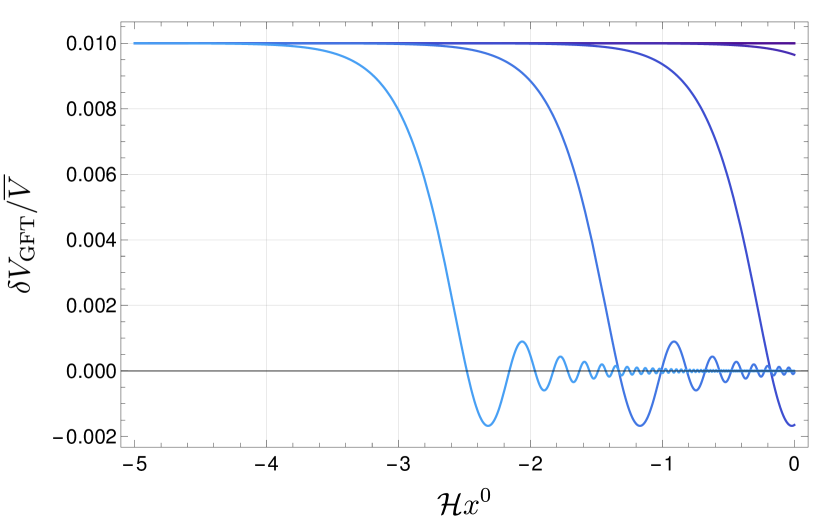
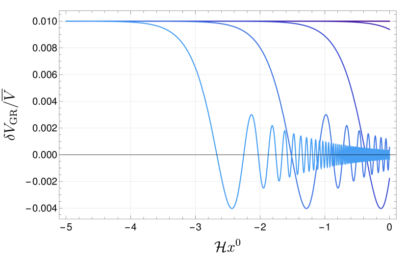
Figure 2: Evolution of relative volume perturbations $\delta V/\bar{V}$ as dictated by GFT, respectively GR. Here, we set the integration constant $c_{1}^{(\mathrm{GR})}=10^{-2}$. Notice, that the quantities $(x^{0},\mathcal{H})$ and $(k,\mathcal{H})$ only appear as a product, respectively a quotient, setting the two scales for the system $\mathcal{H}x^{0}$ and $k/\mathcal{H}$. The drawn momenta lie in the range $k/\mathcal{H}\in\{10^{-3},\;...,\;10^{2}\}$, where lighter blue corresponds to larger modes. Qualitatively, this range captures super-horizon, intermediate and sub-horizon modes, respectively.

The deviations between GFT and GR volume perturbations are two-fold, and become relevant for modes $a^{2}k/\mathcal{H}\gtrsim 1$. First, as the perturbations cross the Hubble horizon, the ratio $(\delta V/\bar{V})_{\mathrm{GFT}}$ is more strongly suppressed by an additional exponential factor of $\textrm{e}^{-3\mathcal{H}x^{0}/2}$. Second, the phase of the two functions is shifted. This becomes apparent by considering an asymptotic expansion of $\delta V/\bar{V}$ in terms of large modes $a^{2}k/\mathcal{H}\gg 1$

$$\left(\frac{\delta V}{\bar{V}}\right)_{\mathrm{GFT}} \;\underset{a^{2}k/\mathcal{H}\gg 1}{\longrightarrow}\;\sqrt{\pi}c_{1}^{\mathrm{GR}}\Gamma\left(\frac{7}{4}\right)\left(\frac{4\mathcal{H}}{k}\right)^{5/4}\textrm{e}^{-5\mathcal{H}x^{0}/2}\sin\left(\frac{\pi}{8}-\frac{a^{2}k}{2\mathcal{H}}\right),$$ (131)

$$\left(\frac{\delta V}{\bar{V}}\right)_{\mathrm{GR}}\;\> \;\underset{a^{2}k/\mathcal{H}\gg 1}{\longrightarrow}\;\sqrt{\pi}c_{1}^{\mathrm{GR}}\left(\frac{4\mathcal{H}}{k}\right)^{1/2}\textrm{e}^{-\mathcal{H}x^{0}}\cos\left(\frac{\pi}{4}-\frac{a^{2}k}{2\mathcal{H}}\right).$$ (132)

We will give a physical interpretation for this sub-horizon deviations at the end of this section.

The initial conditions have been chosen so that the matching of $\delta V_{\mathrm{GFT}}/\bar{V}$ and $\delta V_{\mathrm{GR}}/\bar{V}$ holds for super-horizon modes. Attempting a matching with different initial conditions naturally leads to matching conditions which are inconsistent under relational time-evolution. More precisely, matching the two perturbations at a certain time $x^{0}_{*}$ and at a certain scale $k/\mathcal{H}$ which is not super-horizon, the volume perturbations will only match at this instance of time and show strong deviations for all $x^{0}\neq x^{0}_{*}$. Therefore, we conclude that one obtains the closest matching with initial conditions assigned in the super-horizon regime, which is in fact common practice in standard cosmology Riotto:2002yw ; Baumann:2018muz ; Brandenberger:2003vk ; Dodelson:2003ft ; gorbunov . In the following paragraphs, we will therefore assume that $\delta V/\bar{V}$ is given by Eqs. (129) and (130) for GFT and GR, respectively.

Matter perturbations.

Matter perturbations in GFT and GR are respectively governed by

$$\delta\phi_{\mathrm{GFT}}^{\prime\prime}+a^{4}k^{2}\delta\phi_{\mathrm{GFT}} =\left(-3\mathcal{H}\bar{\phi}+2\bar{\phi}^{\prime}\right)\left(\frac{\delta V}{\bar{V}}\right)_{\mathrm{GFT}}^{\prime},$$ (133)

$$\delta\phi_{\mathrm{GR}}^{\prime\prime}\;\>+a^{4}k^{2}\delta\phi_{\mathrm{GR}}\;\> =0,$$ (134)

where we refer to Appendix C.2 for a derivation of the classical equation. While the GR matter equation forms a closed system, the matter perturbation equation of GFT does not close, since the relative volume perturbation enters as a source term on the right-hand side. However, as we show in this paragraph, these inhomogeneities are controlled by the parameter $c_{1}^{\mathrm{GR}}$. To make this statement explicit, notice that the solution of $\delta\phi_{\mathrm{GR}}$ is given by

$$\delta\phi_{\mathrm{GR}}(x^{0},k)=d_{1}^{\mathrm{GR}}J_{0}\left(\frac{a^{2}k}{2\mathcal{H}}\right).$$ (135)

For simplicity, we set $d_{1}^{\mathrm{GR}}=1$ in the remainder, such that the difference of initial conditions for $\delta\phi$ and $\delta V/\bar{V}$ is captured by $c_{1}^{\mathrm{GR}}$. The differential equation for $\delta\phi_{\mathrm{GFT}}$ is solved numerically. Given initial conditions $\delta\phi_{\mathrm{GFT}}(-5)=d_{1}^{\mathrm{GR}}$ and $\delta\phi_{\mathrm{GFT}}^{\prime}(-5)=0$, the dynamics of GFT and GR matter perturbations show good agreement, as Fig. 3 visualizes. A more direct comparison of the two perturbations for a fixed mode, say $k/\mathcal{H}=10^{3}$, and for varying constant $c_{1}^{\mathrm{GR}}$ is given in Fig. 4.

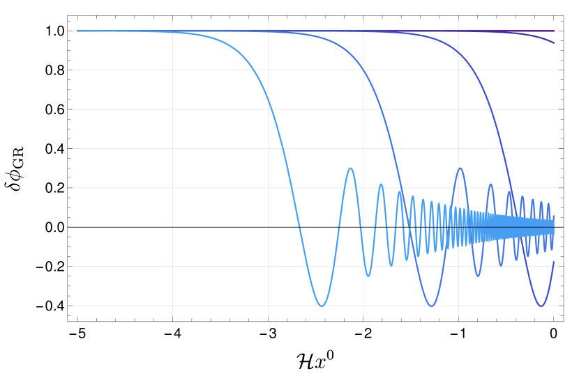
Figure 3: Solutions of matter perturbations derived from GFT and GR, respectively, where we set $d_{1}^{\mathrm{GR}}=1$. In this plot, the modes $k/\mathcal{H}$ lie again in the set $\{10^{-3},\;...,\;10^{2}\}$ with the same color coding as for $\delta V$. Furthermore, the initial condition of the relative volume perturbations is fixed to $c_{1}^{\mathrm{GR}}=10^{-2}$.

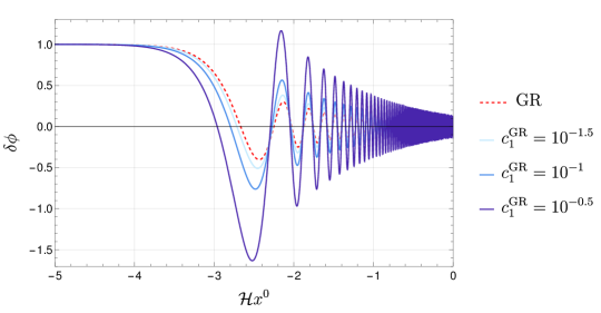
Figure 4: For fixed mode $k/\mathcal{H}=10^{3}$, this plot shows a comparison of the GFT (blue) and GR (dashed red) solutions depending on the value of $c_{1}^{\mathrm{GR}}$. Clearly, the two solutions closely agree for small $c_{1}^{\mathrm{GR}}$.

Curvature-like perturbations.

Similar to the matter perturbations, the equations for the curvature-like perturbation $\tilde{\mathcal{R}}$

$$\tilde{\mathcal{R}}_{\mathrm{GFT}}^{\prime\prime}+a^{4}k^{2}\tilde{\mathcal{R}}_{\mathrm{GFT}} =\left[3\mathcal{H}-\frac{1}{4M_{\mathrm{Pl}}^{2}}\left(\bar{\phi}^{2}\right)^{\prime}\right]\left(\frac{\delta V}{\bar{V}}\right)_{\mathrm{GFT}}^{\prime},$$ (136)

$$\tilde{\mathcal{R}}_{\mathrm{GR}}^{\prime\prime}\;\>+a^{4}k^{2}\tilde{\mathcal{R}}_{\mathrm{GR}}\;\> =0,$$ (137)

derived from GFT and GR, respectively, differ in a source term on the right-hand side of the GFT equation. Since $\tilde{\mathcal{R}}$ is by definition a linear combination of the volume perturbation ratio $\delta V/\bar{V}$ and the matter perturbation $\delta\phi$, the initial conditions must be chosen accordingly.

With the choices for $\delta V_{\mathrm{GR}}/\bar{V}$ and $\delta\phi_{\mathrm{GR}}$ of the previous paragraphs, being $d_{1}^{\mathrm{GR}}=1$ and $c_{1}^{\mathrm{GR}}$ not fixed, the curvature-like perturbation equation of GR is solved by

$$\tilde{\mathcal{R}}_{\mathrm{GR}}=\left(\frac{1}{\sqrt{6}}-\frac{c_{1}^{\mathrm{GR}}}{3}\right)J_{0}\left(\frac{a^{2}k}{2\mathcal{H}}\right).$$ (138)

It is important to notice that $c_{1}^{\mathrm{GR}}$ enters the expression of the classical quantity $\tilde{\mathcal{R}}_{\mathrm{GR}}$ explicitly, in contrast to the classical matter perturbations $\delta\phi_{\mathrm{GR}}$. To find the behavior of $\tilde{\mathcal{R}}_{\mathrm{GFT}}$, we solve its governing differential equation numerically, with initial conditions $\tilde{\mathcal{R}}(-5)=\frac{1}{\sqrt{6}}-\frac{c_{1}^{\mathrm{GR}}}{3}$ and $\tilde{\mathcal{R}}^{\prime}(-5)=0$. The result is depicted on the left-hand side of Fig. 5, next to the analytical solution of GR.

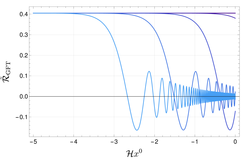
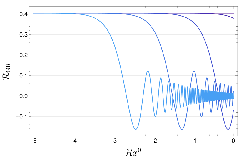
Figure 5: Solutions of curvature-like perturbations $\tilde{\mathcal{R}}$ in GFT and GR, respectively, where the integration constant is fixed to $c_{1}^{\mathrm{GR}}=1$. The range of modes and the associated coloring in the plots are as for $\delta V$ and $\delta\phi$ above.

Matching of GFT and GR solutions is controlled by the parameter $c_{1}^{\mathrm{GR}}$, which now enters both $\tilde{\mathcal{R}}_{\mathrm{GR}}$ and $\tilde{\mathcal{R}}_{\mathrm{GFT}}$. A comparison of the classical and the GFT solutions for a fixed mode $k/\mathcal{H}=10^{3}$ and different values of $c_{1}^{\mathrm{GR}}$ is depicted in Fig. 6. As explained above, $\tilde{\mathcal{R}}_{\mathrm{GFT}}$ is gauge-invariant as a relational quantity, while $\tilde{\mathcal{R}}_{\mathrm{GR}}$ changes under gauge transformations as $\tilde{\mathcal{R}}_{\mathrm{GR}}\mapsto\tilde{\mathcal{R}}_{\mathrm{GR}}+k^{2}\xi$. One can exploit this gauge freedom on the GR side to improve the matching for a fixed mode. However, a consistent improvement of matching between $\tilde{\mathcal{R}}_{\mathrm{GFT}}$ and $\tilde{\mathcal{R}}_{\mathrm{GR}}$ by choosing a certain $\xi$ is not possible for all modes. Therefore, there does not exist a gauge where the matching of GFT and GR perturbations is perfect at all modes.

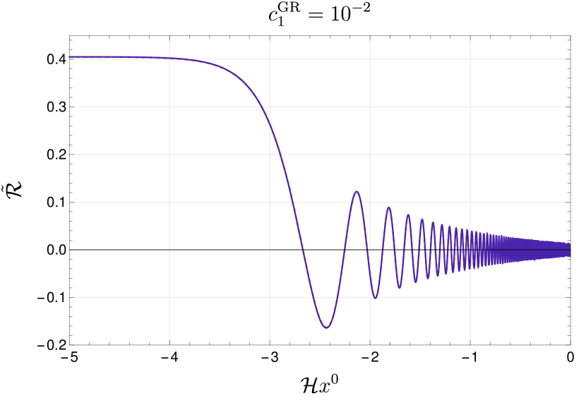
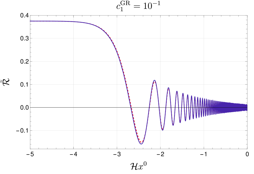
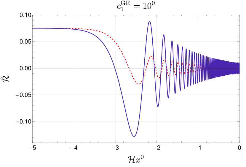
Figure 6: Comparison of classical (dashed red) and GFT solution (blue) for different values of $c_{1}^{\mathrm{GR}}$ at a fixed mode $k/\mathcal{H}=10^{3}$. For $c_{1}^{\mathrm{GR}}=10^{-2}$, the curves show almost perfect matching and are therefore visually indistinguishable.

Summarizing, the GFT perturbation equations for $\delta V/\bar{V}$, $\delta\phi$ and $\tilde{\mathcal{R}}$ do not close in that the relative volume perturbation enters the equations for $\delta\phi$ and $\tilde{\mathcal{R}}$ as a source term. While solution for $\delta V/\bar{V}$ can be fully matched only in the super-horizon limit, both $\delta\phi$ and $\tilde{\mathcal{R}}$ can be matched for a wide range of modes by requiring $c_{1}^{\mathrm{GR}}$ to a small value (as required for the self-consistency of the perturbative setting).

In the last paragraph of this section, we discuss in more detail the sub-horizon regime, which is where the deviations between GFT and GR perturbations are most pronounced.

Sub-horizon and trans-Planckian modes.

In this paragraph, we argue that in the context of classical GR as an effective field theory, sub-horizon modes $a^{2}k/\mathcal{H}\gg 1$ should be naturally considered trans-Planckian, if the cosmological system is relationally described in terms of a physical reference frame made out of four massless scalar fields. Particularly important in this paragraph, we work in units of $8\pi G=1$ and explicitly keep track of factors of Planck masses. Starting this classical analysis, we introduce harmonic coordinates $\chi^{\mu}=\kappa^{\mu}x^{\mu}$ (no summation over $\mu$) Marchetti:2021gcv , with $\kappa^{\mu}$ dimensionful constants. In these coordinates, the energy momentum tensor, defined in Eq. (173), is given by

$$M_{\mathrm{Pl}}^{2}\>T_{\mu\nu}=\sum_{\lambda=0}^{3}(\kappa^{\lambda})^{2}\left(\delta^{\lambda}_{\mu}\delta^{\lambda}_{\nu}-\frac{g_{\mu\nu}}{2}g^{\rho\sigma}\delta^{\lambda}_{\rho}\delta^{\lambda}_{\sigma}\right)+\partial_{\mu}\phi\partial_{\nu}\phi-\frac{g_{\mu\nu}}{2}g^{\rho\sigma}\partial_{\rho}\phi\partial_{\sigma}\phi\,,$$ (139)

with background $(00)$-component

$$M_{\mathrm{Pl}}^{2}\;\bar{T}_{00}=\frac{1}{2}\left(\bar{\pi}_{\phi}^{2}+(\kappa^{0})^{2}+3a^{4}\kappa^{2}\right),$$ (140)

where, $\kappa\equiv\kappa^{i}$, motivated by relational isotropy (see Assumption KS2). Therefore, the constants $\partial_{\mu}\kappa^{i}x^{i}$ already enter at the background level. Notice, that this strongly differs to cosmology in coordinates, where the spatial coordinates only enter the perturbed quantities. At zeroth order in perturbations, the Einstein equations are given by

$$3\mathcal{H}^{2}=\frac{1}{2M_{\mathrm{Pl}}^{2}}\left(\bar{\pi}_{\phi}^{2}+(\kappa^{0})^{2}+3a^{4}\kappa^{2}\right).$$ (141)

As one can check explicitly from e.g. equation (166), following the definition of $\mathcal{H}^{2}$ above, the sub-horizon condition is re-expressed as

$$a^{4}k^{2}\gg\mathcal{H}^{2}\geq\frac{a^{4}\kappa^{2}}{2M_{\mathrm{Pl}}^{2}}.$$ (142)

Now, in order for the coordinates $x^{\mu}$ to have mass dimension of $-1$ (given that $[\chi^{\mu}]=1$), the mass dimension of the $\kappa^{\mu}$ needs to be $2$. Thus, we can re-write $\kappa^{\mu}$ in terms of the Planck-mass and some dimensionless constant $\tilde{\kappa}^{\mu}$, i.e. $\kappa^{\mu}=\tilde{\kappa}^{\mu}M_{\mathrm{pl}}^{2}$. The sub-horizon condition can therefore be recast into

$$\frac{k^{2}}{M_{\mathrm{pl}}^{2}}\gg\tilde{\kappa}^{2}.$$ (143)

Choosing coordinates which are perfectly adapted to the physical scalar reference frame suggests $\tilde{\kappa}=1$, so that we have $\chi^{\mu}=M_{\mathrm{Pl}}^{2}x^{\mu}$. In that case, the sub-horizon condition implies that

$$k^{2}\gg M_{\mathrm{pl}}^{2}\,,$$ (144)

which suggests that the sub-horizon regime is in fact trans-Planckian in the physical reference frame adopted. Importantly, this conclusion is based on the rod contribution to $\bar{T}_{00}$ which, as argued in Appendix C.3, is generic and not only a particular feature of the harmonic coordinate system.

Notice that this issue becomes only apparent when one considers inhomogeneities, since in the homogeneous setting there is no notion of super- and sub-horizon regimes. This is why choosing $\kappa^{\mu}=1$ or $\kappa^{\mu}=M_{\text{pl}}^{2}$ did not make any practical difference in previous studies (e.g. in Oriti:2016qtz $\kappa^{\mu}=1$ was imposed when comparing the effective GFT equations with GR). Clearly, the result that sub-horizon modes are trans-Planckian in the standard effective field theory treatment of linear cosmological perturbations in the relational frame used here calls for a better understanding and further investigations. Specifically, it should be checked if this also holds for the more realistic case of a dust frame. We comment on the relation to the so-called Trans-Planckian Censorship Conjecture (TCC) in Sec. 5.1.

Summary.

Summarizing this section, we compared geometric and matter perturbations in GFT and GR, showing agreement in the super-horizon limit $a^{2}k/\mathcal{H}\ll 1$. For intermediate and sub-horizon modes, one obtains deviations which, for matter perturbations, are small if the initial condition $c_{1}^{\mathrm{GR}}$ is small. $\delta V/\bar{V}$ and $\delta\phi$ can be combined into the curvature-like perturbation $\tilde{\mathcal{R}}$ which agrees in GFT and GR for a wide range of modes if $c_{1}^{\mathrm{GR}}$ is small. Notice, that all three perturbation quantities remain small under relational time evolution, implying that the perturbative framework defined here is in fact self-consistent. Finally, given that (i) sub-horizon modes seem in fact to be associated with a trans-Planckian regime in the physical reference frame we consider and (ii) classical corrections to the standard cosmological perturbation equations coming from the presence of reference fields only enter proportionally to the rod variable $\kappa^{2}$, which in turn can be consistently neglected (see Appendix C.2 for further details), the deviations between the GFT effective continuum dynamics from GR are most naturally interpreted as macroscopic quantum gravity corrections.

5 Summary and conclusion

In this section, we provide a summary and discussion of the main results obtained in this article. First, in Sec. 5.1, we review the main ideas of this work and the procedures applied to obtain our results. Thereafter, in Sec. 5.2, we discuss in more detail the two main results and how these can serve as an important step towards a better understanding of the microscopic nature of cosmic perturbations and towards connecting GFT-perturbations with cosmological observations. Moreover, we provide an overview of pursuing research directions that we consider fruitful.

5.1 Summary

Throughout this article, our explorations have been guided by two overarching principles, both of which are facilitated by the extended causal structure of the complete BC model Jercher:2022mky . The first principle is that the (classical) causal properties of frame fields should be carefully transferred to the quantum theory in order to correctly recast the emerging macroscopic physics in relational terms. The second principle is that non-trivial macroscopic geometries are due to quantum entanglement of microscopic degrees of freedom. In particular, in our model, the inhomogeneities of cosmological observables are the result of (relational) nearest-neighbor two-body entanglement between GFT quanta.

Following the first principle, in Sec. 2.1 we introduced the complete BC GFT model for Lorentzian quantum gravity, including both spacelike and timelike tetrahedra as the fundamental quanta of our theory. This is a minimal framework in which the first principle above can be consistently implemented. The inclusion of timelike tetrahedra necessitates an extension of the Fock space structure, which we realized by means of a tensor product between the spacelike and timelike sector. Crucial for the computation of expectation values, we extended the algebra of creation and annihilation operators to the tensor product Fock space. Still at the level of kinematics, we introduced in Sec. 2.2 five minimally coupled massless scalar fields to the GFT model, serving as a relational frame and matter content, respectively. Here, we made the first guiding principle manifest by restricting the kinetic kernels of the GFT in such a way that the clock and the rods only propagate along timelike, respectively spacelike dual edges. From a discrete gravity perspective, this restricts the gradient of the clock to be timelike and the gradient of the rods to be spacelike.

The second principle was implemented instead in Sec. 3, where we introduced the concept of perturbed coherent peaked states. These extend the concept of spacelike CPSs Marchetti:2020qsq ; Marchetti:2020umh in two ways. At the level of the background, we complemented the spacelike CPS by introducing a condensate (the simplest collective state) also on the timelike sector. The specific form of the condensate wavefunctions and their peaking properties have been guided by geometric and relational isotropy (see Assumption KS2) as well as to simplify the ensuing computations of perturbed observables. The second important difference between these states and the spacelike CPSs is that in the former, perturbations are associated with the action of three types of two-body operators, which encode correlations between and within spacelike and timelike sectors. This is how the second principle above is implemented in our framework. Thereupon, in Sec. 3.3, we derived dynamical equations for the perturbed condensate in a relational manner as the expectation value of the full quantum dynamics with respect to the perturbed CPS.

In Sec. 4, we derived the background and perturbed dynamics of observables by computing expectation values of GFT operators with respect to the perturbed CPS. To compare such emergent quantities to observables of GR, we introduced matching conditions that relate macroscopic GFT observables with quantities commonly used in standard cosmology. At the background level, we reproduced the results of Marchetti:2020umh ; Jercher:2021bie , showing that for late relational times, the dynamics of the spatial volume $\bar{V}$ and the scalar field $\bar{\phi}$ in GFT and GR agree. We computed the dynamics of the perturbed spatial volume $\delta V$ and the perturbed matter field $\delta\phi$ in Secs. 4.1 and 4.3, respectively. Their effective equations show a significant improvement compared to Marchetti:2020umh as the harmonic spatial derivative term of GR, entering with a factor of $a^{4}$, is now faithfully reproduced. Similarly to what is commonly done in standard cosmological perturbation theory, we also combined geometric and matter perturbations into a curvature-like quantity $\tilde{\mathcal{R}}$, the dynamics of which again show an improvement with respect to previous work. Despite the similarities between the effective dynamics of GFT and GR perturbations, deviations in the form of source terms are present in the differential equations for $\delta V,\delta\phi$ and $\tilde{\mathcal{R}}$. To study these differences further we provided a comparison between solutions of perturbations in Sec. 4.5. Remarkably, the curvature-like observable $\tilde{\mathcal{R}}_{\mathrm{GFT}}$ shows good agreement with $\tilde{\mathcal{R}}_{\mathrm{GR}}$ at all scales if initial conditions are chosen appropriately. Differences, though small, are most apparent for sub-horizon modes, which in our relational reference frame appear to be associated with trans-Planckian scales. Together with the arguments of Appendix C.2, this suggests that the deviations between GFT and GR perturbations should in fact be interpreted as quantum gravity effects.

5.2 Discussion and outlook

In this section we discuss the two main results of this work. First, that from the perspective of the underlying quantum gravity theory, cosmological perturbations can be seen as arising from quantum correlations. Second, that the macroscopic effective dynamics of these perturbations show some deviations from GR at scales that we interpret as trans-Planckian in our physical scalar frame.

5.2.1 Cosmological perturbations and quantum entanglement

The first of the two results mentioned above provides crucial insights into the intrinsically quantum nature of cosmological perturbations. Moreover, it concretely substantiates the intuition, shared by many approaches to quantum gravity, that non-trivial geometries are associated with entanglement between the fundamental quantum gravity degrees of freedom, see for instance Ryu:2006bv ; Nishioka:2009un ; Bianchi:2012ev ; Faulkner:2013ica ; Cao:2016mst ; swingle2018spacetime ; colafrancheschi2022emergent ; Bianchi:2023avf .

In this work, entanglement is encoded in relational two-body nearest neighbor correlations between GFT atoms, and it is lifted to the macroscopic level (and thus associated with cosmological quantities) by the properties of two-body coherent states. These states deviate substantially from one-body condensate states and their differences can be seen perturbatively as entangled “out-of-condensate” components. We leave it to future research to investigate the associated entanglement entropy.

We should emphasize, however, that, in this work, this is the only way in which quantum effects have been incorporated into emergent continuum physics, since the microscopic dynamics are still obtained within a mean-field analysis. As we have shown in Appendix B, this is a very robust approximation as long as the GFT interactions are negligible. As noted in Oriti:2016qtz ; Marchetti:2020umh , interactions will eventually become important at very late times, and thus their study will be crucial for determining the self-consistency of the framework. When interactions are present, the inclusion of out-of-condensate perturbations will require a systematic analysis of the quantum properties of the GFT field. This scenario (in the simpler deparametrized setting of Wilson-Ewing:2018mrp ) is studied in Garcia:2023abc by perturbatively splitting the GFT field into a classical homogeneous part and an inhomogeneous quantum field.

Finally, we leave it as an interesting avenue of future research to extend our analysis to microscopically different GFT models. While this work is based on the recent completion of the Barrett-Crane model, it will be highly interesting to study the extent to which our procedure and results carry over to the closely related EPRL model Rovelli:2011eq ; Perez:2012wv , which seeks to provide a covariant quantization of Palatini-Holst gravity in first-order formulation. This will first require the complete formulation of this model as a GFT. Should spacelike and timelike quanta of geometry be part of the condensate phase, which needs to be explicitly checked e.g. via a Landau-Ginzburg analysis, the perturbation theory developed here should in principle be straightforwardly transferable. Since recent results suggest that the BC and EPRL models could lie in the same universality class from the point of view of continuum gravitational physics Asante:2020qpa ; Dittrich:2021kzs ; Asante:2021zzh ; Jercher:2021bie ; Dittrich:2022yoo ; Marchetti:2022igl ; Marchetti:2022nrf , we do not expect substantial differences between the perturbation theory of these two models. However, once our framework will have been extended to also model tensor perturbations, on which we comment below, it will be interesting to check if these modes are anomalously polarized in case of the EPRL model. This can be expected from the parity-oddness of the Holst term and thus of the graviton propagator, see for instance Ashtekar:1988sw ; Freidel:2005sn ; Contaldi:2008yz ; Neiman:2011gf ; Bethke:2011ru ; Bethke:2011kx ; Rovelli:2012yy .

5.2.2 Emergent effective dynamics of cosmological perturbations

The inclusion of timelike tetrahedra allowed us to causally couple the scalar physical frame to the underlying GFT model. This, in turn, played a crucial role in obtaining a form of the effective dynamics of cosmological perturbations which matches the functional form of the GR equations. Note, however, that despite the important role played by timelike tetrahedra, several parameters associated with the timelike sector of our states were not involved at all in the GR matching and are thus completely unconstrained. This “passive” behavior of timelike quanta, exemplified by the fact that the GR matching forces their perturbed number to be trivial (see Sec. 4.2), admits two possible interpretations. First, it could be the mathematical realization of the physical intuition that our universe, by virtue of the Cosmological Principle, can be fully described (at least at the background level) by evolving spacelike quantities only. On the other hand, it could be due to the fact that only spacelike quantities have been considered in this work. If this is the case, one would expect that extending the analysis to other types of geometric observables (especially the extrinsic curvature) would constrain the free parameters of the timelike sector of our states.

However, the presence of such “irrelevant” free parameters in the timelike sector is a blessing in disguise. Indeed, it implies that the emergent perturbation equations are determined by only a set of parameters which turn out to be fixed by the requirement of consistency with the background dynamics. In other words, the predictions made by these models under a mean-field approximation are in principle easily falsifiable by comparison with cosmological observations. There are three different levels (in increasing order of conceptual and computational complexity) at which one could try to make contact with observations.

Phenomenology.

First, one could try to phenomenologically incorporate the modified dynamics of trans-Planckian modes arising from GFT into the Standard Cosmological Model. Since, for an inflationary phase slightly longer than the minimum period, all modes observed today were originally trans-Planckian Brandenberger:2012aj , this could already produce non-trivial observable effects. Note that this would not technically violate the Trans-Planckian Censorship Conjecture (TCC) Bedroya:2019snp ; Bedroya:2019tba ; Brandenberger:2021pzy , since in principle the quantum gravity effects captured by these phenomenological models need not be described in terms of an effective field theory.

Extraction of full cosmological dynamics.

A more systematic approach would be to derive the emergent cosmological perturbation dynamics from the full quantum gravity theory. However, this requires: (i) the construction of additional operators to extract the full effective (anisotropic) geometry, (ii) the inclusion of the appropriate matter content, and (iii) the generalization of the analysis performed here to early times. Let us discuss the above three points in some more detail.

1. The construction of additional geometric operators is extremely important for several reasons. First, it would allow us to extend our analysis to observables commonly used in theoretical and observational cosmology, such as the comoving curvature $\mathcal{R}$. As mentioned in Sec. 4.4, this observable cannot be constructed from the volume operator alone, since the latter is composed of both $\psi$ and $E$, while $\mathcal{R}$ contains only $\psi$. To determine $E$, one would have to relax isotropy (see Assumption KS2) and introduce anisotropic observables, such as the areas of orthogonal two-surfaces. Introducing observables that capture anisotropies and curvature would also be important to reconstruct the full effective metric, including not only scalar perturbations, but also vector and, most importantly (especially for observational purposes), tensor perturbations. Unfortunately, however, the construction of such operators has been mostly hampered by the lack of a graph structure in the GFT Fock space. One way around this problem would be to represent only relational observables in the GFT Fock space. However, a rigorous construction of the latter is also highly non-trivial, as discussed in detail in Marchetti:2020umh . Once these steps have been taken, it is quite conceivable that the modeling of tensor perturbations will also require the inclusion of lightlike tetrahedra, since tensor modes can be expected to propagate along lightlike dual edges. We leave the investigation of these points to future research.

2. Regarding matter, only minimally coupled scalar fields have been systematically included in GFT models and used for cosmological applications Oriti:2016qtz ; Li:2017uao . Particular attention has been paid to massless and free scalar fields, but recently the analysis has been extended to include a non-trivial potential (which is crucial to model e.g. an inflaton-driven early acceleration phase) Ladstatter:2023abc . To move toward a more realistic matter content of the universe, one would have to include cosmic fluids (matter and radiation). Considerable effort has been devoted to the study of dust in classical and quantum gravity (see e.g. Giesel:2012rb ; Domagala:2010bm and Giesel:2007wk ; Giesel:2020bht ; Giesel:2020xnb ; Husain:2020uac for cosmological applications), since it not only constitutes a key component of the Universe, but also serves as a natural physical reference frame. In fact, it is the reference frame in which the Cosmological Principle is formulated, and thus in which background and perturbations are defined. This is a particularly important point, since the mixing between sub-horizon and trans-Planckian modes emphasized in Sec. 4.5 is associated with a definition of background and perturbations with respect to our physical scalar frame. Coupling dust to GFT models would therefore not only allow us to produce more realistic cosmological models, but also to have access to an additional physical reference frame with clear cosmological relevance, in which one could explore delicate issues such as the sub-horizon/trans-Planckian mixing mentioned above. Importantly, it would also allow us to test the physical covariance (or violation thereof) of the emergent cosmological dynamics. As a final comment on this point, we report that matter components may also emerge due to the underlying GFT dynamics, see Oriti:2021rvm for an example.

3. Generalizing the current analysis to earlier times would be important to understand the imprint of the quantum gravity bounce on the perturbations. Moreover, for the perturbation theory developed here to be self-consistent also in this regime it will be important to check if the energy density of the perturbations remains bounded and small compared to the background quantum geometry so that back reaction effects can be ignored. This concerns in particular perturbations of trans-Planckian wavelength and was dubbed the “real trans-Planckian issue” in another setting Agullo:2012sh ; Agullo:2023rqq . In general, however, the mean-field equations become considerably more complicated as the density of the background condensate decreases Marchetti:2021gcv . In particular, recent results Fischer:2023abc seem to suggest that, in the super-horizon limit, the early times emergent dynamics cannot be reconciled with that of any modified gravity theory.

Initial conditions from the fundamental theory.

Finally, in both the methods discussed so far, the primordial power spectrum would be obtained by a Fock quantization of the macroscopic degrees of freedom. This is a strategy that is followed, for example, in both condensed matter physics altland_simons_2010 and LQC Fernandez-Mendez:2012poe ; Fernandez-Mendez:2013jqa ; gomar ; CastelloGomar:2016rjj ; CastelloGomar:2017kbo ; Agullo:2012sh ; Agullo:2012fc ; Agullo:2013ai ; Agullo:2016hap ; Ashtekar:2020gec (see Wilson-Ewing:2016yan ; Agullo:2023rqq for a review). From the perspective of quantum gravity, however, it would be natural to look for a mechanism for generating the cosmological initial conditions that can be derived entirely from the fundamental theory. If the statistical properties of the cosmological inhomogeneities and anisotropies are ultimately due to quantum gravity fluctuations, their description may require going beyond the effective relational framework (which is based on observable averages) used here, and considering relational observables rigorously defined on the GFT Fock space. Similarly, one could explore the possibility that the inflationary mechanism is purely quantum geometric in nature, although this possibility has already been ruled out in some phenomenological GFT models deCesare:2016rsf ; DeSousa:2023tja .

Appendix A List of assumptions

In this appendix, we present an exhaustive list of the assumptions made in order to arrive at the results we obtained in the main body of this work. Naturally, the assumptions can be split into kinematic and dynamic ones. Furthermore, we split the assumptions into two categories, namely structural ones and those stemming from matching with GR perturbations. The former category contains assumptions that are motivated either conceptually or that simplify technically challenging computations.

A.1 Kinematic assumptions

Kinematic approximations are related to the properties of the specific states we are considering.

Structural.

KS1

(Perturbed condensate states): In this paper, we model a spatially homogeneous and isotropic spacetime with scalar perturbations by perturbed condensate states, which extend the notion of usual condensate states Gielen:2013naa ; Gielen:2014ila ; Gielen:2014uga ; Oriti:2015qva ; Gielen:2016dss ; Oriti:2016qtz ; Pithis:2016cxg ; Pithis:2019tvp in two ways. First, given the causally extended structure including timelike tetrahedra, the background contains an additional timelike condensate, introduced in Sec. 3.1.2. Second, perturbations are encoded in $2$-body operators that create an entanglement within and between the spacelike and timelike sector. As discussed in Secs. 5 and Appendix B, this is a first step in the direction of out-of-condensate perturbations.

KS2

(Geometrical and relational isotropy): The spacelike and timelike condensate wavefunctions as well as the correlation functions $\delta\Phi,\delta\Psi$ and $\delta\Xi$ are required to satisfy a quantum analogue of isotropy, realized by setting all the area eigenvalues of the faces $f$ of a tetrahedron to the same value, $\rho_{f}=\rho$. Moreover, the spacelike peaking encoded in the condensate wavefunction $\tau$ is isotropic by choosing the same peaking parameters for all of the three spatial directions. This also ensures that in a derivative expansion for the effective relational equations, only the Laplace operator with respect to the rod variables enters.

KS3

(Peaking and frame-dependence): Following the strategy of Marchetti:2020umh ; Marchetti:2020qsq ; Marchetti:2021gcv , the condensate wavefunction factorizes into a peaking term and a reduced wavefunction. On the spacelike sector, the peaking function only contains the clock variable, while the timelike condensate is peaked on clock and rods. This ensures that the spatial derivative, acting on the volume perturbations, is only associated to spacelike dual edges. The peaking functions are Gaussians with a non-trivial phase and a small width. As argued in Marchetti:2020umh ; Marchetti:2020qsq , a non-vanishing $\epsilon$ as well as a non-vanishing phase are required in order to guarantee that all quantum fluctuations of observables associated to the reference fields are small in the classical regime. Both of the reduced condensate wavefunctions, $\tilde{\sigma}(\chi^{0})$ and $\tilde{\tau}(\chi^{0})$, only depend on relational time as they are assumed to be part of the background. For the $2$-body correlations $\delta\Phi,\delta\Psi$ and $\delta\Xi$, no peaking is encoded and an explicit rod-dependence is assumed in order to render these functions part of the perturbations.

KS4

(Signature of tetrahedra and faces): We extend the spacelike Barrett-Crane model by timelike tetrahedra and leave the inclusion of lightlike tetrahedra for future research. For the timelike condensate, entering the perturbed CPS in Eq. (28), we assume that the corresponding timelike tetrahedra contain spacelike faces only. This assumption is supported by two reasons: $(i)$ Recent studies in Jercher:2023abc suggest that only spacelike faces contribute to a condensate phase and $(ii)$ timelike and spacelike tetrahedra can interact only via spacelike faces, as shown in Jercher:2022mky .

KS5

(Regularization): At several points of the analysis, infinities appear that need to be treated appropriately. Extended closure in Eq. (2) yields empty SL$(2,\mathbb{C})$-integrations in the definition of the GFT action, $2$-body operators and the equations of motion. On the other hand, due to spatial homogeneity and the fact that $\sigma$ is peaked only on the clock, the spacelike background equations in Sec. 3.3.1 as well as the background expectation value of the $3$-volume operator in Sec. 4.1 contain empty rod-integrations. Both types of divergencies are considered as unphysical, and we consider only the finite factors of these expressions.

Motivated by classical matching.

KC1

(Peaking on matter momenta): We assume the condensate wavefunctions $\sigma$ and $\tau$ to be peaked on the matter momentum $\pi_{\phi}$, realized by a Gaussian function without phase. This is necessary in order to recover the Friedmann equations at the background level as well as to render feasible perturbation equations for the condensate and the observables in Secs. 3.3 and 4, respectively. As pointed out in Marchetti:2021gcv , a deeper physical intuition for this peaking may be obtained when considering a scalar field with non-trivial potential.

KC2

(Local perturbation functions): A priori, the $2$-body correlations $\delta\Phi,\delta\Psi$ and $\delta\Xi$ are bi-local functions of the relational reference frame and the matter momentum $\pi_{\phi}$. To make contact to localized perturbations, we assume that the two arguments are identified via a $\delta$-distributions. Following the simplicial gravity picture, this assumption would correspond to correlations within the same $4$-simplex with momentum conservation across tetrahedra.

KC3

(Peaking parameters): To render the computations of Sec. 4 feasible and to allow for a more straightforward matching of GFT and GR perturbations, we assume that the peaking parameters $\epsilon^{\pm}$ and $\pi_{0}^{\pm}$ of the spacelike, respectively the timelike sector are related as $\epsilon^{+}=\epsilon^{-}$ and $\pi_{0}^{+}=-\pi_{0}^{-}$. Furthermore, we assume that the phase parameters $\pi_{x}$ and $\pi_{0}^{+}$ satisfy the strong inequality $\pi_{x}\gg\pi_{0}^{+}$, which yields a drastic simplification for the dynamical equation of the perturbed volume in Eq. (75).

A.2 Dynamic assumptions

Dynamic approximations are related to the details of the GFT action and on how background and perturbed equations for the condensate and the observables are obtained.

Structural.

DS1

(GFT action and causal building blocks): We choose to work with an extension of the Lorentzian Barrett-Crane model Jercher:2021bie ; Jercher:2022mky and here study its cosmological implications while including spacelike and timelike tetrahedra and excluding lightlike ones. Thus, the configurations are the two group fields $\varphi_{+}$ and $\varphi_{-}$ which are distinguished in their domain and in the form of the simplicity constraint, given in Eq. (3).

DS2

(Scalar field coupling): Clock and rod fields $\chi^{\mu}$ as well as the matter field $\phi$ are coupled to the GFT such that the Feynman amplitudes correspond to a simplicial gravity path integral with the fields propagating along dual edges. As discussed in Li:2017uao , this coupling is obtained in a semi-classical limit, which is an assumption that should be kept mind. In order to turn the scalar reference frame into a physical Lorentzian reference frame, we align its causal character with that of the geometry by imposing restrictions on the kernels in Eqs. (26). As elaborated in Sec. 2.2, the physical picture of these conditions is that the clock propagates along timelike dual edges and the rods propagate along spacelike dual edges.

DS3

(Mean-field dynamics): We assume the effective dynamics to be well approximated by the mean-field equations. In fact, as we show in Appendix B and discuss in the conclusion, the mean-field equations solve the higher-order Schwinger-Dyson equations if negligible interactions and linear perturbation theory is assumed.

DS4

(Negligible interactions): When taking expectation values with respect to the perturbed CPS $\ket{\Delta;x^{0},{\bf\it x}}$, interaction terms are expected to be negligible in the effective dynamics. It has been shown in Oriti:2016qtz , that the error induced by this assumption grows with the number of GFT particles. This assumption can therefore be consistently implemented at late but not very late times. See also Gielen:2013naa for a complementary discussion on this matter.

DS5

(Classical matter content): We assume that the matter content of the classical theory, given by the five fields $\chi^{\mu}$ and $\phi$, is dominated by $\phi$. In this way, perturbations of $\chi^{\mu}$ are considered to be negligible and inhomogeneities of matter and geometry can be defined unambiguously with respect to the clock and rod fields. In Appendix C.2, we compute the corrections to the classical Einstein equations if one would not neglect the frame contributions to the energy-momentum tensor.

Motivated by classical matching.

DC1

(Mesoscopic regime): Classical dynamics are obtained in a mesoscopic regime, where the averaged number of particles of the system is taken to be large enough to allow for both a continuum interpretation of the expectation values of relevant operators and classical behavior, but not too large that interactions are dominating. Furthermore, the perturbation equations of Sec. 3.3 and 4 simplify significantly in this regime, as the condensate wavefunctions are solved by simple exponential functions, see Eqs. (49) and (50).

DC2

(Single-spin dominance): We assume that coefficients of $\sigma,\tau$ and the $2$-body correlations $\delta\Phi,\delta\Psi$ and $\delta\Xi$ in spin representation are dominated by a single representation label $\rho$, mostly suppressed in the notation. For the background condensates, this assumption is supported by the studies of Ref. Gielen:2016uft ; Pithis:2016wzf ; Pithis:2016cxg ; Jercher:2021bie , which show that under rather generic assumptions on the kinetic kernels of the GFT, a dominant representation emerges dynamically.

DC3

(Dynamical freedom): Exploiting the dynamical freedom of having two first-order equations for three functions, we relate the spacelike-spacelike correlation $\delta\Phi$ and the spacelike-timelike correlation $\delta\Psi$ via a function $\mathrm{f}$. This function is chosen such that the dynamical equation for $\delta\Psi$ as well as the definition of $\delta V$ simplify drastically. Finally, when matching the $a^{4}$-term in front of the spatial derivative of $\delta V$ in Eq. (75), the function $\mathrm{f}$ is fixed completely. As we detail in Sec. 5.2, it is left open for future studies to include interactions (see for instance Ref. Garcia:2023abc for further details) such that the number of independent first-order equations matches the number of perturbations functions and no such dynamical freedom is present.

DC4

(Constant phase): Splitting the perturbation function $\delta\Psi$ into modulus $R$ and phase $\Theta$, we assume the phase to be constant, rendering the dynamical equations of $\delta\Psi$ and $\delta V$ feasible. Moreover, $\Theta$ is set to $n\frac{\pi}{2}$ in Sec. 4.1, simplifying the dynamical equation for $\delta V$ in Eq. (75). One can show that if one relaxes the constant-$\Theta$ condition to a pure time dependence, then consistency requires that $\Theta$ is in fact constant. Clearly, the most general case is given for $\Theta$ carrying a space dependence. However, the resulting equations of motion for the perturbation function as well as for observables take a highly intricate form, which does not allow for further analytical studies.

DC5

(Normalized scale factor): As commonly done in standard cosmology, the scale factor $a$ is normalized to $1$ at present relational time, such that it takes smaller values for all earlier relational times. Notice, that this assumption is not in contradiction with a large GFT-particle number or, equivalently, a large volume. That is because the volume is given by $a^{3}$ times a fiducial volume factor, which can be much larger than one.

DC6

(Timelike particle number): When computing the dynamics of matter observables, we assumed that the effective mass parameters of the spacelike and timelike sector satisfy $\mu_{+}>\mu_{-}$. This assumption is guided by the intuition that the background is predominantly described by the spacelike condensate. Indeed, as a consequence, one finds that the background number of spacelike GFT-particles dominates over the timelike particle number in the classical limit. In Sec. 4.3, this leads to a simplification of the emergent equations for the perturbed matter field $\delta\phi$ and the perturbed matter momentum $\delta\pi_{\phi}$.

Appendix B Going beyond mean-field in the absence of interactions

In this appendix, we show that in the absence of interactions, higher order Schwinger-Dyson equations reduce to powers of the lowest mean-field equation. This result is of interest for the perturbed coherent states introduced in Sec. 3.2, as these states constitute out-of-condensate perturbations only if interactions are taken into account. Furthermore, this result is exactly the reason for the dynamical freedom of one of the $2$-body correlation functions which we exploited in Sec. 4 to match the perturbations of GR.

For a polynomially bounded functional $\mathcal{O}[\varphi_{\alpha},\bar{\varphi}_{\alpha}]$ on field space, where $\alpha$ refers to either the spacelike or the timelike group field, the Schwinger-Dyson equations are given by

$$\expectationvalue{\functionalderivative{\mathcal{O}}{\bar{\varphi}_{\alpha}}-\mathcal{O}\functionalderivative{S}{\bar{\varphi}_{\alpha}}}=0.$$ (145)

The polynomial expansion of the operator $\mathcal{O}$ is given by

$$\mathcal{O}[\varphi_{\alpha},\bar{\varphi}_{\alpha}]=\sum_{k,l,m,n}\mathcal{O}_{klmn}\;\bar{\varphi}_{+}^{k}\varphi_{+}^{l}\otimes\bar{\varphi}_{-}^{m}\varphi_{-}^{n},$$ (146)

with $\mathcal{O}_{klmn}$ being the kernel. Given the perturbed state $\ket{\Delta}$, defined in Sec. 3.2, the expectation value of $\mathcal{O}$ up to first order in perturbations is schematically given by

$$\expectationvalue{\mathcal{O}}{\Delta}=\evaluated{\mathcal{O}}_{\sigma,\tau}+\left(2\evaluated{\bar{\varphi}_{+}\functionalderivative{\mathcal{O}}{\varphi_{+}}}_{\sigma,\tau}+\evaluated{\functionalderivative[2]{\mathcal{O}}{\varphi_{+}}}_{\sigma,\tau}\right)\delta\Phi\;+$$ (147)

$$+ \left(\evaluated{\bar{\varphi}_{-}\functionalderivative{\mathcal{O}}{\varphi_{+}}}_{\sigma,\tau}+\evaluated{\bar{\varphi}_{+}\functionalderivative{\mathcal{O}}{\varphi_{-}}}_{\sigma,\tau}\right)\delta\Psi+\left(2\evaluated{\bar{\varphi}_{-}\functionalderivative{\mathcal{O}}{\varphi_{+}}}_{\sigma,\tau}+\evaluated{\functionalderivative[2]{\mathcal{O}}{\varphi_{-}}}_{\sigma,\tau}\right)\delta\Xi+\mathrm{c.c.},$$

where a vertical line indicates that the operator $\mathcal{O}$ is functionally evaluated on the condensate wavefunctions $\sigma$ and $\tau$.

Building up on this result, we consider now the Schwinger-Dyson equation under the assumption that interactions are absent, i.e. $S=\sum_{\alpha}\bar{\varphi}_{\alpha}\mathcal{K}_{\alpha}\varphi_{\alpha}$. At zeroth order, the equations then take the form

$$\evaluated{\functionalderivative{\mathcal{O}}{\bar{\varphi}_{\alpha}}}_{\sigma,\tau}=\evaluated{\mathcal{O}\mathcal{K}_{\alpha}\varphi_{\alpha}}_{\sigma,\tau},$$ (148)

which, for $\mathcal{O}=\mathbbm{1}$, reproduces the mean-field equation studied in Sec. 3.3.1.

At first order, we look at the coefficients in front of the same perturbation function. For instance, the $\delta\Psi$-term is given by

$$\evaluated{\bar{\varphi}_{-}\frac{\delta^{2}\mathcal{O}}{\delta\varphi_{+}\delta\bar{\varphi}_{\alpha}}}_{\sigma,\tau}+\evaluated{\bar{\varphi}_{+}\frac{\delta^{2}\mathcal{O}}{\delta\varphi_{-}\delta\bar{\varphi}_{\alpha}}}_{\sigma,\tau}=\evaluated{\bar{\varphi}_{-}\frac{\delta(\mathcal{O}\mathcal{K}_{\alpha}\varphi_{\alpha})}{\delta\varphi_{+}}}_{\sigma,\tau}+\evaluated{\bar{\varphi}_{+}\frac{\delta(\mathcal{O}\mathcal{K}_{\alpha}\varphi_{\alpha})}{\delta\varphi_{-}}}_{\sigma,\tau},$$ (149)

with the other coefficients given in a similar form. Clearly, upon solutions of the zeroth order equation, also the first-order equations are satisfied. Hence, higher-order Schwinger-Dyson equations do not yield additional dynamical equations if one works $(i)$ in a perturbative setting and $(ii)$ in the absence of interactions. As a consequence, we find in the analysis of the $2$-body correlation functions in Sec. 3.3 a dynamical freedom for one of the variables. The results of this appendix suggest that in order to obtain higher-order out-of-condensate equations, one would need to take interactions into account. We comment on this matter further in Sec. 5.

Appendix C Classical perturbation theory

In this appendix, we provide an overview of the perturbation equations for geometry and matter in classical general relativity. In order to allow for a simpler comparison with relational GFT results, we mostly use harmonic coordinates $\{x^{\mu}\}$ which are adapted to the reference field $\{\chi^{\mu}\}$ via the relation $\chi^{\mu}=\kappa^{\mu}x^{\mu}$ (no summation over $\mu$), where $\kappa^{\mu}$ are some dimensionful proportionality factors Gielen:2018fqv . In harmonic coordinates, the reference fields are assumed to satisfy the Klein-Gordon equation at all orders of perturbations. This can equivalently be re-written as a condition on the metric,

$$\Gamma^{\lambda}_{\mu\nu}g^{\mu\nu}=0.$$ (150)

C.1 Geometry

At zeroth order, the line element of a spatially flat FLRW spacetime is given by

$$\differential{s}^{2}=\bar{g}_{\mu\nu}\differential{x}^{\mu}\differential{x}^{\nu}=-N^{2}\differential{t}^{2}+a^{2}\differential{{\bf\it x}}^{2},$$ (151)

where $N$ is the lapse function, $a$ is the scale factor and $\differential{{\bf\it x}}^{2}$ the line element of $3$-dimensional Euclidean flat space. Imposing harmonic gauge on the background yields $N=c_{0}a^{3}$, where $c_{0}$ is an integration constant. For the remainder of this subsection, we set $c_{0}=1$, and we assume that the matter content is dominated by the matter field $\phi$ with conjugate momentum $\pi_{\phi}$.

Within these assumptions and in units where $8\pi G=1$, the dynamics of the geometry at background level are captured by

$$3\mathcal{H}^{2}=\frac{1}{2M_{\mathrm{Pl}}^{2}}\bar{\pi}_{\phi}^{2},\qquad\mathcal{H}^{\prime}=0,$$ (152)

where $\mathcal{H}=a^{\prime}/a$ is the Hubble parameter and $\bar{\pi}_{\phi}$ is the background contribution of the canonical conjugate of the scalar field, defined in Eq. (178). Introducing the background volume $\bar{V}=a^{3}$, the geometric equations can be recast to

$$3\left(\frac{\bar{V}^{\prime}}{3\bar{V}}\right)^{2}=\frac{1}{2M_{\mathrm{Pl}}^{2}}\bar{\pi}_{\phi}^{2},\qquad\left(\frac{\bar{V}^{\prime}}{3\bar{V}}\right)^{\prime}=0.$$ (153)

To derive perturbed volume equations from GR, we consider in the following first-order scalar perturbations of the FLRW metric. Using the background harmonic gauge condition, the line element is given by

$$\differential{s}^{2}=-a^{6}(1+2A)\differential{t}^{2}+a^{4}\partial_{i}B\differential{t}\differential{x^{i}}+a^{2}\left((1-2\psi)\delta_{ij}+2\partial_{i}\partial_{j}E\right)\differential{x}^{i}\differential{x}^{j},$$ (154)

with scalar perturbation functions $A,B,\psi$ and $E$. Einstein’s equations at linear order yield Marchetti:2021gcv ; Battarra:2014tga

$$\frac{1}{2M_{\mathrm{Pl}}^{2}}\bar{\phi}^{\prime}\delta\phi^{\prime}+3\mathcal{H}\psi^{\prime}-a^{4}\nabla^{2}\psi-\mathcal{H}\nabla^{2}\left(E^{\prime}-a^{2}B\right) =0,$$ (155)

$$\mathcal{H}A+\psi^{\prime}-\frac{1}{2M_{\mathrm{Pl}}^{2}}\bar{\phi}^{\prime}\delta\phi =0,$$ (156)

$$E^{\prime\prime}-a^{4}\nabla^{2}E =0,$$ (157)

where $\delta\phi$ is the scalar field perturbation. Combining Eq. (155) and the time-derivative of Eq. (156), we obtain

$$\psi^{\prime\prime}=-\mathcal{H}A^{\prime}-3\mathcal{H}\psi^{\prime}+a^{4}\nabla^{2}\psi+\mathcal{H}\nabla^{2}\left(E^{\prime}-a^{2}B\right).$$ (158)

To obtain an equation for the perturbed volume, which is an observable accesible also from the GFT side, consider on a slice of constant time the local volume element

$$\sqrt{-g_{(3)}}=\bar{V}+\delta V=a^{3}\left(1-3\psi+\nabla^{2}E\right).$$ (159)

Thus, we identify the perturbed spatial volume as

$$\frac{\delta V}{\bar{V}}=-3\psi+\nabla^{2}E.$$ (160)

Taking the second derivative of $\delta V/\bar{V}$ and using Eqs. (157) and (158), one obtains

$$\left(\frac{\delta V}{\bar{V}}\right)^{\prime\prime}+3\mathcal{H}\left(\frac{\delta V}{\bar{V}}\right)^{\prime}-a^{4}\nabla^{2}\left(\frac{\delta V}{\bar{V}}\right)=3\mathcal{H}\left(A^{\prime}+a^{2}\nabla^{2}B\right).$$ (161)

Harmonic gauge.

At first order in perturbations, the harmonic gauge conditions given by Battarra:2014tga

$$0 =A^{\prime}+3\psi^{\prime}-\nabla^{2}(E^{\prime}-a^{2}B),$$ (162a)

$$0 =(a^{2}B)^{\prime}+a^{4}(A-\psi-\nabla^{2}E),$$ (162b)

which, imposed on Einstein’s equations (155) - (157), yields Battarra:2014tga ; Marchetti:2021gcv

$$\psi^{\prime\prime}-a^{4}\nabla^{2}\psi =0, A^{\prime\prime}-a^{4}\nabla^{2}A+4a^{4}\nabla^{2}\psi=0\,$$ (163)

$$E^{\prime\prime}-a^{4}\nabla^{2}E =0, (a^{2}B)^{\prime\prime}-a^{4}\nabla^{2}(a^{2}B)-8a^{2}(a^{2}\psi)^{\prime}=0.$$ (164)

Expressed in terms of the volume, the first harmonic gauge condition is expressed as

$$A^{\prime}+a^{2}\nabla^{2}B=\left(\frac{\delta V}{\bar{V}}\right)^{\prime},$$ (165)

such that the volume equation becomes

$$\left(\frac{\delta V}{\bar{V}}\right)^{\prime\prime}-a^{4}\nabla^{2}\left(\frac{\delta V}{\bar{V}}\right)=0.$$ (166)

or equivalently

$$\delta V^{\prime\prime}-6\mathcal{H}\delta V^{\prime}+9\mathcal{H}^{2}\delta V-a^{4}\nabla^{2}\delta V=0.$$ (167)

To change to Fourier space in the rod variable, heavily employed in Sec. 4, one can simply perform the substitution $\nabla^{2}\rightarrow-k^{2}$ here and in the following.

Following Battarra:2014tga , there is a residual gauge freedom in performing a coordinate transformation

$$\xi^{\mu}\mapsto x^{\mu}+\xi^{\mu},$$ (168)

with $\xi^{\mu}=(\xi^{0},\partial^{i}\xi)$ satisfying

$$(\xi^{0})^{\prime\prime}-a^{4}\nabla^{2}\xi^{0}=\xi^{\prime\prime}-a^{4}\nabla^{2}\xi=0,$$ (169)

such that harmonicity is conserved. Under this transformation, the perturbation functions transform as Battarra:2014tga ; Marchetti:2020umh

$$\psi\mapsto\psi+\mathcal{H}\xi^{0}, A\mapsto A-(\xi^{0})^{\prime}-3\mathcal{H}\xi^{0},$$ (170)

$$E\mapsto E-\xi, B\mapsto B+a^{2}\xi^{0}-a^{-2}\xi^{\prime}.$$ (171)

After introducing the matter equations in the following, we combine the geometric and matter quantities in a single fully gauge-invariant quantity, the so-called curvature perturbation $\mathcal{R}$.

C.2 Matter

The matter content of the classical theory consists of four reference scalar fields $\chi^{\mu}$ as well as one additional free minimally coupled real scalar field $\phi$, defined by the continuum action

$$S[\chi^{\mu},\phi]=-\frac{1}{2M_{\mathrm{Pl}}^{2}}\int\differential[4]{x}\sqrt{-g}g^{ab}\left(\partial_{a}\phi\partial_{b}\phi+\sum_{\mu=0}^{3}\partial_{a}\chi^{\mu}\partial_{b}\chi^{\mu}\right).$$ (172)

The energy momentum tensor in arbitrary coordinates is given by

$$M_{\mathrm{Pl}}^{2}\;T_{ab}=\sum_{\lambda=0}^{3}\left(\partial_{a}\chi^{\lambda}\partial_{b}\chi^{\lambda}-\frac{g_{ab}}{2}g^{mn}\partial_{m}\chi^{\lambda}\partial_{n}\chi^{\lambda}\right)+\partial_{a}\phi\partial_{b}\phi-\frac{g_{ab}}{2}g^{mn}\partial_{m}\phi\partial_{n}\phi.$$ (173)

For the remainder of this subsection, we use harmonic coordinates. Also, we assume that the matter content is dominated by the matter field $\phi$. The full equations of motion for $\phi$ are given by the massless Klein-Gordon equation

$$\partial_{\mu}\left(\sqrt{-g}g^{\mu\nu}\partial_{\nu}\phi\right)=0.$$ (174)

Linearizing in both, the scalar field and the metric, we obtain the zeroth order equation

$$\bar{\phi}^{\prime\prime}=0.$$ (175)

and the first-order perturbation equation

$$\delta\phi^{\prime\prime}-a^{4}\nabla^{2}\delta\phi=\left[A^{\prime}+3\psi^{\prime}-\nabla^{2}E^{\prime}+a^{2}\nabla^{2}B\right]\bar{\phi}^{\prime},$$ (176)

respectively. Supplementing the latter with the harmonic gauge condition in Eq. (162a), $\delta\phi$ satisfies

$$\delta\phi^{\prime\prime}-a^{4}\nabla^{2}\delta\phi=0.$$ (177)

To define the GR counterpart of the GFT observables $\hat{\Pi}_{\phi}^{\alpha}$, defined in Eq. (96), we introduce the momentum conjugate to the scalar field, commonly defined as

$$\pi_{\phi}^{\mu}\vcentcolon=\partialderivative{\tilde{\mathcal{L}}}{(\partial_{\mu}\phi)}=-\sqrt{-g}g^{\mu\nu}(\partial_{\nu}\phi),$$ (178)

where $\tilde{\mathcal{L}}$ is the Lagrangian density, defined by the matter field action above. Expanding up to linear order, the scalar field momentum $\pi_{\phi}^{\mu}$ is given by

$$\pi^{\mu}_{\phi}=-\overline{\sqrt{-g}}\bar{g}^{\mu 0}\partial_{0}\bar{\phi}-\delta\sqrt{-g}\bar{g}^{\mu 0}\partial_{0}\bar{\phi}-\overline{\sqrt{-g}}\left(\delta g^{\mu 0}\partial_{0}\bar{\phi}+\bar{g}^{\mu\nu}\partial_{\nu}\delta\phi\right),$$ (179)

which can be split into background and perturbed part

$$\pi_{\phi}^{\mu}=\bar{\pi}_{\phi}^{\mu}+\delta\pi_{\phi}^{\mu}.$$ (180)

At the background level and in harmonic gauge, $\bar{\pi}_{\phi}^{\mu}$ is given by

$$\bar{\pi}_{\phi}^{0}=\partial_{0}\bar{\phi},\qquad\bar{\pi}_{\phi}^{i}=0.$$ (181)

The perturbed part of $\pi_{\phi}^{\mu}$ is given by

$$\delta\pi_{\phi}^{0} =\left(-A-3\psi+\nabla^{2}E\right)\bar{\phi}^{\prime}+\delta\phi^{\prime},$$ (182)

$$\delta\pi_{\phi}^{i} =a^{2}\bar{\phi}^{\prime}\partial^{i}B-a^{4}\partial^{i}\delta\phi.$$ (183)

Applying the zeroth- and first-order equations for $\phi$, the perturbed momentum satisfies the relativistic energy-momentum conservation equation

$$\partial_{\mu}\delta\pi_{\phi}^{\mu}=\left(\delta\pi_{\phi}^{0}\right)^{\prime}+\partial_{i}\delta\pi_{\phi}^{i}=0.$$ (184)

Re-expressing this equation in terms of observables that are available in GFT, being $\bar{V},\delta V,\bar{\phi}$ and $\delta\phi$, we find

$$\left(\delta\pi_{\phi}^{0}\right)^{\prime}-\delta\phi^{\prime\prime}-\left(\frac{\delta V}{\bar{V}}\right)^{\prime}\bar{\phi}^{\prime}=-A^{\prime}\bar{\phi}^{\prime}.$$ (185)

While the left-hand side is given in terms of variables available in GFT, the right-hand side contains the variable $A$, which is not accessible by the GFT observable that are available at the present state. In Sec. 5.2, We comment on the importance of defining additional geometrical observables in GFT.

Classsical Mukhanov-Sasaki-like equation.

As the transformations of Eqs. (170) and (171) show, the harmonic gauge conditions leaves a residual gauge freedom. Under these transformations, the perturbed scalar field $\delta\phi$ changes as

$$\delta\phi\mapsto\delta\phi-\bar{\phi}^{\prime}\xi^{0}.$$ (186)

Given this transformation behavior, one can combine $\psi$ and $\delta\phi$ to a fully gauge-invariant quantity, the so called gauge-invariant curvature perturbation

$$\mathcal{R}\vcentcolon=\psi+\mathcal{H}\frac{\delta\phi}{\bar{\phi}^{\prime}}.$$ (187)

Since in harmonic gauge, $\psi$ and $\delta\phi$ satisfy the same equation, $\mathcal{R}$ satisfies Battarra:2014tga

$$\mathcal{R}^{\prime\prime}-a^{4}\nabla^{2}\mathcal{R}=0.$$ (188)

In the context of GFT, one does not have direct access to the quantity $\psi$ but rather to the perturbed volume $\delta V$. For comparison of classical and GFT mechanics, we define the curvature-like perturbation $\tilde{\mathcal{R}}$ as

$$\tilde{\mathcal{R}}\vcentcolon=-\frac{\delta V}{3\bar{V}}+\mathcal{H}\frac{\delta\phi}{\bar{\phi}^{\prime}}.$$ (189)

Again, since $\delta V/\bar{V}$ and $\delta\phi$ satisfy the same equation, $\tilde{\mathcal{R}}$ obeys

$$\tilde{\mathcal{R}}^{\prime\prime}-a^{4}\nabla^{2}\tilde{\mathcal{R}}=0.$$ (190)

Notice however, that $\tilde{\mathcal{R}}$ is not gauge invariant but changes as

$$\tilde{\mathcal{R}}\mapsto\tilde{\mathcal{R}}-\nabla^{2}\xi.$$ (191)

Still, since $\xi$ is assumed to satisfy the equation above, the equation for $\tilde{\mathcal{R}}$ does not change under gauge transformations.

Reference field corrections to the perturbation equations.

In this Appendix, we have so far assumed that the matter content is dominated by the scalar field $\phi$, neglecting contributions of the clock and rod fields $\chi^{\mu}$. However, in order to rule out the possibility that the source term in the GFT perturbation equations (82), (118) and (122) is associated to the a potential contribution of they physical reference frame, it is instructive to consider the background and perturbed field equations with all matter terms, similarly to what has been done e.g. in Husain:2020uac (albeit with a different physical frame).

At the background level, the Einstein equations take the form

$$3\mathcal{H}^{2}=\frac{1}{2M_{\mathrm{Pl}}^{2}}\left(\bar{\phi}^{\prime 2}+(\kappa^{0})^{2}+3\kappa^{2}a^{4}\right),\qquad\mathcal{H}^{\prime}=\frac{1}{M_{\mathrm{Pl}}^{2}}\kappa^{2}a^{4},$$ (192)

which are readily dependent. Clearly, if one assumes $\pi_{\phi}^{2}$ to dominate, consistency requires $\mathcal{H}^{\prime}=0$.

To compute the perturbed Einstein equations, we add the frame contributions to the perturbed energy-momentum tensor, the components of which are explicitly given by

$$M_{\mathrm{Pl}}^{2}\;\tensor{(\delta T^{\chi})} =\frac{(\kappa^{0})^{2}}{a^{6}}A-\frac{\kappa^{2}}{a^{2}}(3\psi-\nabla^{2}E),$$ (193)

$$M_{\mathrm{Pl}}^{2}\;\tensor{(\delta T^{\chi})}{{}^{0}_{i}} =\frac{\kappa^{2}}{a^{4}}\partial_{i}B,$$ (194)

$$M_{\mathrm{Pl}}^{2}\;\tensor{(\delta T^{\chi})}{{}^{i}_{j}} =\delta^{i}_{j}\left(-\frac{(\kappa^{0})^{2}}{a^{6}}A+\frac{\kappa^{2}}{a^{2}}(-\psi+\nabla^{2}E)\right)-2\frac{\kappa^{2}}{a^{2}}\partial^{i}\partial_{j}E.$$ (195)

Using the Einstein tensor components of Battarra:2014tga , the perturbed equations of motion are given by

$$\frac{1}{2M_{\mathrm{Pl}}^{2}}\bar{\phi}^{\prime 2}+3\mathcal{H}\psi^{\prime}-a^{4}\nabla^{2}\psi-\mathcal{H}\nabla^{2}(E^{\prime}-a^{2}B)+\frac{1}{2M_{\mathrm{Pl}}^{2}}a^{4}\kappa^{2}(3(A+\psi)-\nabla^{2}E) =0,$$ (196)

$$\mathcal{H}A+\psi^{\prime}+\frac{1}{2M_{\mathrm{Pl}}^{2}}\left(\kappa^{2}a^{2}B-\bar{\phi}^{\prime}\delta\phi\right) =0,$$ (197)

$$E^{\prime\prime}-a^{4}\nabla^{2}E+\frac{2}{M_{\mathrm{Pl}}^{2}}\kappa^{2}a^{4}E =0,$$ (198)

complemented by the harmonic gauge conditions in Eqs. (162). Already at this point, one observes that the clock contributions, entering with $(\kappa^{0})^{2}$, will cancel out upon the background equations as these only enter with the perturbation function $A$. We leave a clarification of this intriguing cancellation open for future investigations.

Following similar steps as above, we obtain a differential equation for $\psi$

$$\psi^{\prime\prime}-a^{4}\nabla^{2}\psi+\frac{2}{M_{\mathrm{Pl}}^{2}}\kappa^{2}a^{4}(A+\psi)=0,$$ (199)

that is modified by the presence of the rod contribution, entering with $\kappa^{2}$. Using the definition of the relative perturbed volume as well as Eqs. (198) and (199), we obtain

$$\left(\frac{\delta V}{\bar{V}}\right)^{\prime\prime}-a^{4}\nabla^{2}\left(\frac{\delta V}{\bar{V}}\right)=-\frac{2}{M_{\mathrm{Pl}}^{2}}\kappa^{2}a^{4}\left(\frac{\delta V}{\bar{V}}-3A\right),$$ (200)

which is modified compared to Eq. (166) by a term that is controlled via the rod variable $\kappa$.

The equation for the perturbed matter field $\delta\phi$ is not altered by the additional clock and rod contributions. Thus, using the volume and matter equation, we obtain an equation for $\tilde{\mathcal{R}}$ in the presence of frame contributions:

$$\tilde{\mathcal{R}}^{\prime\prime}-a^{4}\nabla^{2}\tilde{\mathcal{R}}=\frac{2}{M_{\mathrm{Pl}}^{2}}\kappa^{2}a^{4}\left[\tilde{\mathcal{R}}-A+3\frac{\mathcal{H}}{\bar{\phi}^{\prime}}\delta\phi+2\frac{\delta\phi^{\prime}}{\bar{\phi}^{\prime}}\right].$$ (201)

Clearly, all of the corrections compared to Eq. (189) enter with the rod-variable $\kappa$ and contain a mixture of geometric and matter perturbations. Structurally, these corrections are therefore quite different from those obtained in Husain:2020uac , possibly as a result of the different gauge-fixing. Importantly, this result substantiates the interpretation of the source terms in the perturbation equations obtained from GFT that we give in Sec. 4.5. That is, the source terms are not artifacts of reference frame contributions but are rather interpreted as genuine quantum gravity corrections.

C.3 Change of gauge

In ordinary cosmology, formulated without the use of reference fields as relational coordinates, the most commonly used coordinates are so-called conformal-longitudinal (CL). In this section, we discuss the change from harmonic to CL-coordinates and the consequences for the interpretation of clock and rod fields. To start with, the line element is given by maggiorebook ; Dodelson:2003ft

$$\differential{s}^{2}=a^{2}(\tau)\left[-(1+2\Psi(\tau,{\bf\it x}))\differential{\tau}^{2}+(1-2\Phi(\tau,{\bf\it x}))\differential{{\bf\it x}}^{2}\right],$$ (202)

in CL-coordinates, where $\Psi$ and $\Phi$ and the gauge-invariant Bardeen variables. In order to transform from harmonic coordinates $\{x_{\mathrm{H}}^{\mu}\}$ to CL-coordinates $\{x_{\mathrm{CL}}^{\mu}\}$, we have to perform two transformations, first at the background to conformal time and then a transformation at the level of perturbations. For the background transformation we consider

$$x_{\mathrm{H}}^{0}\rightarrow\tau(x_{\mathrm{H}}^{0})=\int\limits_{0}^{x_{\mathrm{H}}^{0}}\differential{\tilde{x}^{0}}a^{2}(\tilde{x}^{0}),$$ (203)

such that $a^{2}\differential{x_{\mathrm{H}}^{0}}=\differential{\tau}$.

Following Eqs. (170) and (171), the perturbation functions change upon the conformal transformation as

$$\psi\mapsto\psi+H\zeta^{0}, A\mapsto A-\derivative{\tau}\zeta^{0}-3H\zeta^{0},$$ (204)

$$E\mapsto E-\xi, B\mapsto B+\zeta^{0}-\derivative{\tau}\xi,$$ (205)

where we introduced the re-scaled variable $\zeta^{0}=a^{2}\xi^{0}$. The line element of Eq. (202) is then obtained via the transformation

$$\zeta^{0} =E^{\prime}-B,$$ (206)

$$\xi =E.$$ (207)

where A and $\psi$ transform to

$$A \longmapsto A-3H(E^{\prime}-B)-(E^{\prime}-B)^{\prime}\equiv\Psi,$$ (208)

$$\psi \longmapsto\psi+H(E^{\prime}-B)\equiv-\Phi.$$ (209)

Indeed as one can easily verify, the perturbation functions $\Psi$ and $\Phi$ are fully gauge-invariant.

In the new coordinates, the gauge-invariant curvature satisfies

$$\derivative[2]{\mathcal{R}}{\tau}+2H\derivative{\mathcal{R}}{\tau}-\nabla^{2}\mathcal{R}=0,$$ (210)

where $H=\frac{1}{a}\derivative{a}{\tau}$ is the Hubble parameter with respect to conformal time. Since $\tilde{\mathcal{R}}$ is, in contrast to $\mathcal{R}$, not gauge-invariant, it changes under the transformation above to

$$\tilde{\mathcal{R}}\longmapsto\tilde{\mathcal{R}}-\nabla^{2}E.$$ (211)

However, since the equation for $E$ in Eq. (157) is valid manifestly (not only in harmonic gauge) and is the same as that of $\mathcal{R}$, the equation for $\tilde{\mathcal{R}}$ in conformal-longitudinal gauge is given by

$$\derivative[2]{\tilde{\mathcal{R}}}{\tau}+2H\derivative{\tilde{\mathcal{R}}}{\tau}-\nabla^{2}\tilde{\mathcal{R}}=0.$$ (212)

As a result, $\tilde{\mathcal{R}}$ satisfies the same equation in harmonic and CL-coordinates, but solutions of $\tilde{\mathcal{R}}$ change accordingly.

We consider next the four reference fields $\{\chi^{\mu}\}$, which satisfy the Klein-Gordon (KG) equation

$$\partial_{a}\left(\sqrt{-g}g^{ab}\partial_{b}\right)\chi^{\mu}=0.$$ (213)

In harmonic coordinates, we chose adapted solutions of the form $\chi^{\mu}=\kappa^{\mu}x^{\mu}$. Plugging this ansatz into the KG equation, one re-obtains the harmonic gauge conditions

$$c^{\mu}=\partial_{\alpha}\left(\sqrt{-g}g^{\alpha\beta}\partial_{\beta}\right)\kappa^{\mu}x^{\mu}\overset{!}{=}0.$$ (214)

Crucially, since coordinates do in general not transform as scalars nor do the four constraints $c^{\mu}$. That can also be seen by the relation of $c^{\mu}$ and the Christoffel-symbols, $c^{\mu}=\Gamma^{\mu}_{\alpha\beta}g^{\alpha\beta}$, which are well-known to not transform as tensors. As a consequence, $c^{\mu}=0$ is only satisfied in harmonic gauge and is violated in general in other coordinates $\{x^{a}\}$, i.e. $c^{\mu}(x^{a})\neq 0$.

The behavior of clocks and rods differs significantly in different coordinates. To see that explicitly, note that the ansatz $\chi^{0}=\kappa^{0}x^{0}$ is only a solution of the KG-equation in harmonic coordinates and is invalid in particular in conformal-longitudinal coordinates. In contrast, plugging the ansatz $\chi^{i}=\kappa^{i}x^{i}_{\mathrm{CL}}$ into the KG-equation in conformal-longitudinal coordinates yields

$$\partial_{i}\left(\sqrt{-g}g^{ij}\partial_{j}\chi^{l}\right)=\kappa^{l}\partial_{i}\left[a^{2}(1+\Psi-\Phi)\delta^{ij}\partial_{j}x^{l}_{\text{CL}}\right]=a^{4}\kappa^{l}\partial_{l}(\Psi-\Phi)=0\,,$$ (215)

where expanded the geometry up to first order. The last equation above holds true on-shell and by assuming vanishing shear which is the case in our system.

Consequently, when plugging the on-shell solution $\chi^{i}=\kappa^{i}x^{i}_{\mathrm{CL}}$ into the energy-momentum tensor, the background components $\bar{T}_{\mu\nu}(x_{\mathrm{CL}})$ contain a contribution of the rods. Explicitly, we find in CL-coordinates the inequalities

$$k^{2}\gg H^{2}\geq\frac{\kappa^{2}}{2M_{\mathrm{Pl}}^{2}},$$ (216)

where $H$ is again the Hubble parameter in conformal time, such that for $\kappa=M_{\mathrm{Pl}}^{2}$, one obtains

$$k^{2}\gg M_{\mathrm{Pl}}^{2}.$$ (217)

Following the arguments of the last paragraph of Sec. 4.5, these inequalities show the mixing of sub-horizon and trans-Planckian modes. Concluding, the computations of this section demonstrate that the observations of Sec. 4.5 are not a particular feature of harmonic coordinates but are also present using the commonly used conformal-longitudinal coordinates.

Appendix D Derivation of condensate dynamics

In this appendix we provide the detailed derivations of the dynamical equations for the perturbed condensate introduced in Sec. 3.2. To that end, we consider an expansion of the kinetic kernels

$$\mathcal{K}_{+}((\chi^{0})^{2},\pi_{\phi}^{2}) =\sum_{n=0}^{\infty}\frac{\mathcal{K}_{+}^{(2n)}(\pi_{\phi}^{2})}{(2n)!}(\chi^{0})^{2n},$$ (218)

$$\mathcal{K}_{-}(\absolutevalue{{\bf\it\chi}}^{2},\pi_{\phi}^{2}) =\sum_{n=0}^{\infty}\frac{\mathcal{K}_{-}^{(2n)}(\pi_{\phi}^{2})}{(2n)!}\absolutevalue{{\bf\it\chi}}^{2n},$$ (219)

the existence of which is supported by the studies of Li:2017uao . Notice that the reference fields are coupled to the GFT model via the Eqs. (26a) and (26b), such that their expansion differs slightly from that discussed in Marchetti:2021gcv . The reduced condensate wavefunctions $\tilde{\sigma}$ and $\tilde{\tau}$ are expanded in derivatives

$$\tilde{\sigma}(\chi^{0}+x^{0},\pi_{\phi}) =\sum_{n=0}^{\infty}\frac{\tilde{\sigma}^{(n)}(x^{0},\pi_{\phi})}{n!}(\chi^{0})^{n},$$ (220)

$$\tilde{\tau}(\chi^{0}+x^{0},\pi_{\phi}) =\sum_{n=0}^{\infty}\frac{\tilde{\tau}^{(n)}(x^{0},\pi_{\phi})}{n!}(\chi^{0})^{n},$$ (221)

where $\tilde{\sigma}^{(n)}$ denotes the $n$-th derivative with respect to the clock argument, applying similarly to $\tilde{\tau}$. These expansion will be employed both, for the background as well as the perturbed part of the equations of motion.

D.1 Background equations

Spacelike part.

Using the expansions of Eqs. (218) and (220), the (regularized) spacelike background equation (43) evaluates to

$$0 =\int\differential{\chi^{0}}\mathcal{K}_{+}((\chi^{0})^{2},\pi_{\phi}^{2})\tilde{\sigma}(\chi^{0}+x^{0},\pi_{\phi})\eta_{\epsilon^{+}}(\chi^{0},\pi_{0}^{+})$$ (222)

$$=\sum_{m,n}\frac{\mathcal{K}_{+}^{(2m)}(\pi_{\phi}^{2})\tilde{\sigma}^{(n)}(x^{0},\pi_{\phi})}{(2m)!n!}\int\differential[4]{\chi}\eta_{\epsilon^{+}}(\chi^{0},\pi_{0}^{+})(\chi^{0})^{2m+n}$$

$$\approx\mathcal{K}_{+}^{(0)}\left[\left(I_{0}+I_{2}\frac{\mathcal{K}_{+}^{(2)}}{2\mathcal{K}_{+}^{(0)}}\right)\tilde{\sigma}(x^{0},\pi_{\phi})+I_{1}\partial_{0}\tilde{\sigma}(x^{0},\pi_{\phi})+\frac{1}{2}I_{2}\partial_{0}^{2}\tilde{\sigma}(x^{0},\pi_{\phi})\right]\int\differential[3]{\chi},$$

Following Marchetti:2021gcv , we introduced the function $I_{2m+n}(\epsilon^{+},\pi_{0}^{+})$, defined as the $\chi^{0}$ integration, which can be explicitly evaluated to

$$I_{n}(\epsilon^{+},\pi_{0}^{+})=\mathcal{N}_{\epsilon^{+}}\sqrt{2\pi\epsilon^{+}}\left(i\sqrt{\frac{\epsilon^{+}}{2}}\right)^{n}\textrm{e}^{-z_{+}^{2}}H_{n}\left(\sqrt{\frac{\epsilon^{+}}{2}}\pi_{0}^{+}\right),$$ (223)

where $H_{n}$ are the Hermite polynomials and $z_{+}^{2}=\epsilon^{+}(\pi_{0}^{+})^{2}/2$. We truncated the expansion at order $\epsilon^{+}$, leading to the condition that only terms with $2m+n\leq 2$ contribute. Introducing the quantities

$$E_{+}^{2}(\pi_{\phi}) \vcentcolon=\frac{2}{\epsilon^{+}(2z_{+}^{2}-1)}-\frac{\mathcal{K}_{+}^{(2)}}{\mathcal{K}_{+}^{(0)}},$$ (224)

$$\tilde{\pi}_{0}^{+} \vcentcolon=\frac{\pi_{0}^{+}}{2z_{+}^{2}-1},$$ (225)

we finally obtain

$$\partial_{0}^{2}\tilde{\sigma}(x^{0},\pi_{\phi})-2i\tilde{\pi}_{0}^{+}\partial_{0}\tilde{\sigma}(x^{0},\pi_{\phi})-E_{+}^{2}(\pi_{\phi})\tilde{\sigma}(x^{0},\pi_{\phi})=0.$$ (226)

Timelike part.

On the timelike sector, the procedure to obtain the equations of motion differs slightly because of the different peaking properties of $\tau$ and the mere rod-dependence of the timelike kernel $\mathcal{K}_{-}$. Starting with Eq. (44) and inserting the expansions of Eqs. (219) and (221), we obtain

$$0 =\int\differential[4]{\chi}\mathcal{K}_{-}(\absolutevalue{{\bf\it\chi}}^{2},\pi_{\phi}^{2})\tilde{\tau}(\chi^{0}+x^{0},\pi_{\phi})\eta_{\epsilon^{-}}(\chi^{0},\pi_{0}^{-})\eta_{\delta}(\absolutevalue{{\bf\it\chi}},\pi_{x})$$ (227)

$$=\sum_{n}\frac{\tilde{\tau}^{(n)}(x^{0},\pi_{\phi})}{n!}\int\differential{\chi^{0}}\eta_{\epsilon^{-}}(\chi^{0},\pi_{0}^{-})(\chi^{0})^{n}\int\differential[3]{\chi}\mathcal{K}_{-}(\absolutevalue{{\bf\it\chi}}^{2},\pi_{\phi})\eta_{\delta}(\absolutevalue{{\bf\it\chi}},\pi_{x}).$$

Assuming that the spatial integral is non-zero, the equations factorize. Truncating at linear order in $\epsilon^{-}$ finally yields

$$I_{0}^{-}\tilde{\tau}(x^{0},\pi_{\phi})+I_{1}^{-}\partial_{0}\tilde{\tau}(x^{0},\pi_{\phi})+\frac{1}{2}I_{2}^{-}\partial_{0}^{2}\tilde{\tau}(x^{0},\pi_{\phi})\approx 0,$$ (228)

where $I_{n}^{-}$ is defined equivalently to Eq. (223) but evaluated on the timelike peaking parameters $\epsilon^{-}$ and $\pi_{0}^{-}$. Introducing

$$E_{-}^{2} \vcentcolon=\frac{2}{\epsilon^{-}(2z_{-}^{2}-1)},$$ (229)

$$\tilde{\pi}_{0}^{-} \vcentcolon=\frac{\pi_{0}^{-}}{2z_{-}^{2}-1},$$ (230)

the background equation for the timelike reduced condensate wavefunction reads

$$\partial_{0}^{2}\tilde{\tau}(x^{0},\pi_{\phi})-2i\tilde{\pi}_{0}^{-}\partial_{0}\tilde{\tau}(x^{0},\pi_{\phi})-E_{-}^{2}\tilde{\tau}(x^{0},\pi_{\phi})=0.$$ (231)

Notice that due to the interplay of peaking and kernel dependencies, the quantity $E_{-}$ does not carry a matter momentum dependence, in cotrast to $E_{+}(\pi_{\phi})$.

D.2 Perturbation equations

Continuing the analysis of the equations of motion, we derive in this section the perturbed equations of motion for the spacelike and then the timelike sector.

Spacelike part.

Starting point is Eq. (51), which we complement by the peaking properties of the condensate wavefunctions $\sigma$ and $\tau$. As for the background, we expand $\mathcal{K}_{+},\tilde{\sigma}$ and $\tilde{\tau}$ according to Eqs. (218), (220) and (221). Also we use the relation of $\delta\Psi$ and $\delta\Phi$ in Eq. (53) and the relation of peaking parameters in Eq. (55). Truncating then at linear order in $\epsilon^{+}$ and $\delta$, one obtains

$$0 =\mathcal{K}_{+}^{(0)}(p_{\phi}^{2})\Bigg{[}\left(I_{0}+I_{2}\frac{\mathcal{K}_{+}^{(2)}}{2\mathcal{K}_{+}^{(0)}}\right)\delta\Psi\left(J_{0,{\bf\it 0}}\bar{\tilde{\tau}}+f\textrm{e}^{i\theta_{f}}\bar{\tilde{\sigma}}\right)+I_{1}\partial_{0}\left(\delta\Psi(J_{0,{\bf\it 0}}\bar{\tilde{\tau}}+f\textrm{e}^{i\theta_{f}}\bar{\tilde{\sigma}})\right)$$ (232)

$$+\frac{I_{2}}{2}\partial_{0}^{2}\left(\delta\Psi(J_{0,{\bf\it 0}}\bar{\tilde{\tau}}+f\textrm{e}^{i\theta_{f}}\bar{\tilde{\sigma}})\right)+\bar{\tilde{\tau}}I_{0}\frac{J_{0,(0,0,2)}}{2}\nabla_{{\bf\it x}}^{2}\delta\Psi\Bigg{]}.$$

All fields, $\tilde{\sigma}$, $\tilde{\tau}$ and $\delta\Psi$ are evaluated at $x^{0}$, respectively $x^{i}$ and the peaked matter momentum $p_{\phi}$. Notice that the first-order time derivative enters with a coefficient $I_{1}$ and not its complex conjugated because of the the relation between $\pi_{0}^{+}$ and $\pi_{0}^{-}$ as well as the phase factor of the function f in Eq. (54). The functions $I_{0}$ and $I_{2}$ are the functions of temporal peaking parameters defined in the section above, evaluated on the $+$-parameters. Due to the spatial peaking of the timelike condensate $\tau$, coefficients $J_{m,(n_{1},n_{2},n_{3})}$ appear in the expression above, defined as

$$J_{m,(n_{1},n_{2},n_{3})}=\int\differential[3]{\chi}\eta_{\delta}(\absolutevalue{{\bf\it\chi}},\pi_{x})\absolutevalue{{\bf\it\chi}}^{2m}\prod_{i=1}^{3}(\chi^{i})^{n_{i}}.$$ (233)

The relevant coefficients for the derivation of the equations of motion are $J_{0,{\bf\it 0}}$, $J_{2,{\bf\it 0}}$ and $J_{0,(0,0,2)}$, explicitly defined as Marchetti:2021gcv

$$J_{0,{\bf\it 0}} =-2\mathcal{N}_{\delta}\sqrt{2\pi}\pi^{2}\delta^{3/2}z^{2}\textrm{e}^{-z^{2}},$$ (234)

$$J_{2,{\bf\it 0}} =4\mathcal{N}_{\delta}\sqrt{2\pi}\pi^{2}\delta^{5/2}z^{4}\textrm{e}^{-z^{2}},$$ (235)

$$J_{0,(0,0,2)} =\frac{16}{3}\mathcal{N}_{\delta}\sqrt{2\pi}\pi\delta^{5/2}z^{4}\textrm{e}^{-z^{2}},$$ (236)

keeping only first-order contributions in the peaking parameter $\delta$, where $z^{2}=\delta\pi_{x}^{2}/2$.

Factorizing $I-2/2$ from the spacelike perturbed equations of motion above, we finally obtain

$$0 =\partial_{0}^{2}\left(\delta\Psi(J_{0,{\bf\it 0}}\bar{\tilde{\tau}}+f\textrm{e}^{i\theta_{f}}\bar{\tilde{\sigma}})\right)-2i\tilde{\pi}_{0}^{+}\partial_{0}\left(\delta\Psi(J_{0,{\bf\it 0}}\bar{\tilde{\tau}}+f\textrm{e}^{i\theta_{f}}\bar{\tilde{\sigma}})\right)+$$ (237)

$$-E_{+}^{2}\delta\Psi\left(J_{0,{\bf\it 0}}\bar{\tilde{\tau}}+f\textrm{e}^{i\theta_{f}}\bar{\tilde{\sigma}}\right)+\alpha\tilde{\tau}\nabla_{{\bf\it x}}^{2}\delta\Psi,$$

where the parameter $\alpha$ is defined as

$$\alpha\vcentcolon=\frac{I_{0}J_{0,(0,0,2)}}{I_{2}}.$$ (238)

Timelike part.

To derive the perturbed condensate equation on the timelike sector, given in Eq. (59), our starting point is Eq. (58). We use the expansions of Eqs. (219), (220) and (221) as well as the relations of Eqs. (53) and (55) to arrive at

$$0 =\int\differential[3]{\chi}\mathcal{K}_{-}(\absolutevalue{\chi}^{2},p_{\phi}^{2})\left[I_{0}\delta\Psi\bar{\tilde{\sigma}}+\bar{I}_{1}\partial(\delta\Psi\bar{\tilde{\sigma}})+\frac{I_{2}}{2}\partial_{0}^{2}\left(\delta\Psi\bar{\tilde{\sigma}}\right)\right]$$ (239)

$$+\mathcal{K}_{-}^{(0)}(p_{\phi}^{2})\Bigg{[}\left(I_{0}J_{0,{\bf\it 0}}+I_{0}J_{2,{\bf\it 0}}\frac{\mathcal{K}_{-}^{(2)}}{\mathcal{K}_{-}^{(0)}}\right)\delta\Xi\bar{\tilde{\tau}}+J_{0,{\bf\it 0}}I_{1}\partial\left(\delta\Xi\bar{\tilde{\tau}}\right)$$

$$+J_{0,{\bf\it 0}}\frac{I_{2}}{2}\partial_{0}^{2}\left(\delta\Xi\bar{\tilde{\tau}}\right)+I_{0}\frac{J_{0,(0,0,2)}}{2}\bar{\tilde{\tau}}\nabla_{{\bf\it x}}^{2}\delta\Xi\Bigg{]},$$

where the coefficients $I_{0},I_{2},J_{0,\mathbf{0}},J_{2,{\bf\it 0}}$ and $J_{0,(0,0,2)}$ are defined as above. Using the background equations of motion in the classical limit, with solutions given by Eqs. (49) and (50), and factorizing $J_{0,{\bf\it 0}}I_{2}/2$, one obtains

$$0 =\bar{\tilde{\sigma}}\int\differential[3]{\chi}\mathcal{K}_{-}(\absolutevalue{{\bf\it\chi}},p_{\phi}^{2})\left[\left(\frac{2I_{0}}{I_{2}}+(\pi_{0}^{+})^{2}+\mu_{+}^{2}\right)\delta\Psi+2\mu_{+}\partial_{0}\delta\Psi+\partial_{0}^{2}\delta\Psi\right]$$ (240)

$$+\mathcal{K}_{-}^{(0)}J_{0,{\bf\it 0}}\bar{\tilde{\tau}}\Bigg{[}\left(\frac{2I_{0}}{I_{2}}+\frac{I_{0}J_{2,{\bf\it 0}}}{I_{2}J_{0,{\bf\it 0}}}\frac{\mathcal{K}_{-}^{(2)}}{\mathcal{K}_{-}^{(0)}}+(\pi_{0}^{+})^{2}+\mu_{-}^{2}\right)+2\mu_{-}\partial_{0}\delta\Xi+\partial_{0}^{2}\delta\Xi+\frac{\alpha}{J_{0,{\bf\it 0}}}\nabla_{{\bf\it x}}^{2}\delta\Xi\Bigg{]}.$$

Using the definition of $\mu_{-}^{2}$ and introducing

$$\beta\vcentcolon=-\frac{I_{0}J_{2,{\bf\it 0}}}{I_{2}J_{0,{\bf\it 0}}}\frac{\mathcal{K}_{-}^{(2)}}{\mathcal{K}_{-}^{(0)}},\qquad\gamma\vcentcolon=\frac{\alpha}{J_{0,{\bf\it 0}}},$$ (241)

the perturbed equation of motion on the timelike sector is finally given by

$$0 =\bar{\tilde{\sigma}}\int\differential[3]{\chi}\mathcal{K}_{-}(\absolutevalue{{\bf\it\chi}},p_{\phi}^{2})\left[\partial_{0}^{2}\delta\Psi+2\mu_{+}\partial_{0}\delta\Psi-\frac{\mathcal{K}_{+}^{(2)}}{\mathcal{K}_{+}^{(0)}}\delta\Psi\right]$$ (242)

$$+\bar{\tilde{\tau}}\mathcal{K}_{-}^{(0)}J_{0,{\bf\it 0}}\Bigg{[}\partial_{0}^{2}\delta\Xi+2\mu_{-}\partial_{0}\delta\Xi-\beta\delta\Xi+\gamma\nabla_{{\bf\it x}}^{2}\delta\Xi\Bigg{]}.$$

References

- (1) Planck collaboration, Planck 2018 results. VI. Cosmological parameters, Astron. Astrophys. 641 (2020) A6 [1807.06209].
- (2) D. Oriti, The Bronstein hypercube of quantum gravity, in Beyond Spacetime, N. Huggett, K. Matsubara and C. Wüthrich, eds., pp. 25–52 (2020), DOI [1803.02577].
- (3) D. Oriti, Levels of spacetime emergence in quantum gravity, 1807.04875.
- (4) C. Rovelli, What Is Observable in Classical and Quantum Gravity?, Class. Quant. Grav. 8 (1991) 297.
- (5) P.A. Hoehn, A.R.H. Smith and M.P.E. Lock, Trinity of relational quantum dynamics, Phys. Rev. D 104 (2021) 066001 [1912.00033].
- (6) C. Rovelli, Partial observables, Phys. Rev. D 65 (2002) 124013 [gr-qc/0110035].
- (7) B. Dittrich, Partial and complete observables for canonical general relativity, Class. Quant. Grav. 23 (2006) 6155 [gr-qc/0507106].
- (8) M. Domagala, K. Giesel, W. Kaminski and J. Lewandowski, Gravity quantized: Loop Quantum Gravity with a Scalar Field, Phys. Rev. D 82 (2010) 104038 [1009.2445].
- (9) K. Giesel and T. Thiemann, Scalar Material Reference Systems and Loop Quantum Gravity, Class. Quant. Grav. 32 (2015) 135015 [1206.3807].
- (10) J.D. Brown and K.V. Kuchar, Dust as a standard of space and time in canonical quantum gravity, Phys. Rev. D 51 (1995) 5600 [gr-qc/9409001].
- (11) K.V. Kuchar and J.D. Romano, Gravitational constraints which generate a lie algebra, Phys. Rev. D 51 (1995) 5579 [gr-qc/9501005].
- (12) J. Bicak and K.V. Kuchar, Null dust in canonical gravity, Phys. Rev. D 56 (1997) 4878 [gr-qc/9704053].
- (13) K. Giesel, S. Hofmann, T. Thiemann and O. Winkler, Manifestly Gauge-Invariant General Relativistic Perturbation Theory. I. Foundations, Class. Quant. Grav. 27 (2010) 055005 [0711.0115].
- (14) K. Giesel, S. Hofmann, T. Thiemann and O. Winkler, Manifestly Gauge-invariant general relativistic perturbation theory. II. FRW background and first order, Class. Quant. Grav. 27 (2010) 055006 [0711.0117].
- (15) L. Marchetti and D. Oriti, Effective relational cosmological dynamics from Quantum Gravity, JHEP 05 (2021) 025 [2008.02774].
- (16) L. Freidel, Group field theory: An Overview, Int. J. Theor. Phys. 44 (2005) 1769 [hep-th/0505016].
- (17) D. Oriti, The Group field theory approach to quantum gravity, gr-qc/0607032.
- (18) S. Carrozza, Tensorial methods and renormalization in Group Field Theories, Ph.D. thesis, Orsay, LPT, 2013. 1310.3736. 10.1007/978-3-319-05867-2.
- (19) S. Carrozza, Flowing in Group Field Theory Space: a Review, SIGMA 12 (2016) 070 [1603.01902].
- (20) P. Di Francesco, P.H. Ginsparg and J. Zinn-Justin, 2-D Gravity and random matrices, Phys. Rept. 254 (1995) 1 [hep-th/9306153].
- (21) R. Gurau and J.P. Ryan, Colored Tensor Models - a review, SIGMA 8 (2012) 020 [1109.4812].
- (22) R. Gurau, Random Tensors, Oxford University Press (2016).
- (23) D. Oriti, The microscopic dynamics of quantum space as a group field theory, in Foundations of Space and Time: Reflections on Quantum Gravity, pp. 257–320, 10, 2011 [1110.5606].
- (24) A. Ashtekar and J. Lewandowski, Background independent quantum gravity: A Status report, Class. Quant. Grav. 21 (2004) R53 [gr-qc/0404018].
- (25) D. Oriti, Group field theory as the 2nd quantization of Loop Quantum Gravity, Class. Quant. Grav. 33 (2016) 085005 [1310.7786].
- (26) D. Oriti, J.P. Ryan and J. Thürigen, Group field theories for all loop quantum gravity, New J. Phys. 17 (2015) 023042 [1409.3150].
- (27) A. Perez, Spin foam models for quantum gravity, Class. Quant. Grav. 20 (2003) R43 [gr-qc/0301113].
- (28) A. Perez, The Spin Foam Approach to Quantum Gravity, Living Rev. Rel. 16 (2013) 3 [1205.2019].
- (29) V. Bonzom, Spin foam models for quantum gravity from lattice path integrals, Phys. Rev. D 80 (2009) 064028 [0905.1501].
- (30) A. Baratin and D. Oriti, Group field theory with non-commutative metric variables, Phys. Rev. Lett. 105 (2010) 221302 [1002.4723].
- (31) A. Baratin and D. Oriti, Quantum simplicial geometry in the group field theory formalism: reconsidering the Barrett-Crane model, New J. Phys. 13 (2011) 125011 [1108.1178].
- (32) A. Baratin and D. Oriti, Group field theory and simplicial gravity path integrals: A model for Holst-Plebanski gravity, Phys. Rev. D 85 (2012) 044003 [1111.5842].
- (33) M. Finocchiaro and D. Oriti, Spin foam models and the Duflo map, Class. Quant. Grav. 37 (2020) 015010 [1812.03550].
- (34) R. Loll, Discrete approaches to quantum gravity in four-dimensions, Living Rev. Rel. 1 (1998) 13 [gr-qc/9805049].
- (35) J. Ambjorn, A. Goerlich, J. Jurkiewicz and R. Loll, Nonperturbative Quantum Gravity, Phys. Rept. 519 (2012) 127 [1203.3591].
- (36) S. Jordan, Globally and locally causal dynamical triangulations, [Sl: sn] (2013).
- (37) R. Loll, Quantum Gravity from Causal Dynamical Triangulations: A Review, Class. Quant. Grav. 37 (2020) 013002 [1905.08669].
- (38) D. Oriti, Disappearance and emergence of space and time in quantum gravity, Stud. Hist. Phil. Sci. B 46 (2014) 186 [1302.2849].
- (39) S. Gielen, D. Oriti and L. Sindoni, Cosmology from Group Field Theory Formalism for Quantum Gravity, Phys. Rev. Lett. 111 (2013) 031301 [1303.3576].
- (40) D. Oriti, D. Pranzetti and L. Sindoni, Horizon entropy from quantum gravity condensates, Phys. Rev. Lett. 116 (2016) 211301 [1510.06991].
- (41) L. Marchetti, D. Oriti, A.G.A. Pithis and J. Thürigen, Mean-Field Phase Transitions in Tensorial Group Field Theory Quantum Gravity, Phys. Rev. Lett. 130 (2023) 141501 [2211.12768].
- (42) A.G.A. Pithis and J. Thürigen, Phase transitions in group field theory: The Landau perspective, Phys. Rev. D 98 (2018) 126006 [1808.09765].
- (43) L. Marchetti, D. Oriti, A.G.A. Pithis and J. Thürigen, Phase transitions in tensorial group field theories: Landau-Ginzburg analysis of models with both local and non-local degrees of freedom, JHEP 21 (2020) 201 [2110.15336].
- (44) D. Benedetti, J. Ben Geloun and D. Oriti, Functional Renormalisation Group Approach for Tensorial Group Field Theory: a Rank-3 Model, JHEP 03 (2015) 084 [1411.3180].
- (45) J. Ben Geloun, R. Martini and D. Oriti, Functional Renormalization Group analysis of a Tensorial Group Field Theory on , EPL 112 (2015) 31001 [1508.01855].
- (46) D. Benedetti and V. Lahoche, Functional renormalization group approach for tensorial group field theory: a rank-6 model with closure constraint, Classical And Quantum Gravity 33 (2016) [1508.06384].
- (47) J. Ben Geloun, R. Martini and D. Oriti, Functional renormalization group analysis of tensorial group field theories on , Phys. Rev. D 94 (2016) 024017 [1601.08211].
- (48) A.G.A. Pithis and J. Thürigen, (No) phase transition in tensorial group field theory, Phys. Lett. B 816 (2021) 136215 [2007.08982].
- (49) A.G.A. Pithis and J. Thürigen, Phase transitions in TGFT: functional renormalization group in the cyclic-melonic potential approximation and equivalence to O models, JHEP 12 (2020) 159 [2009.13588].
- (50) J.B. Geloun, A.G.A. Pithis and J. Thürigen, QFT with Tensorial and Local Degrees of Freedom: Phase Structure from Functional Renormalization, 2305.06136.
- (51) J. Berges, N. Tetradis and C. Wetterich, Nonperturbative renormalization flow in quantum field theory and statistical physics, Phys. Rept. 363 (2002) 223 [hep-ph/0005122].
- (52) B. Delamotte, An Introduction to the nonperturbative renormalization group, Lect. Notes Phys. 852 (2012) 49 [cond-mat/0702365].
- (53) P. Kopietz, L. Bartosch and F. Schütz, Introduction to the functional renormalization group, vol. 798 (2010), 10.1007/978-3-642-05094-7.
- (54) N. Dupuis, L. Canet, A. Eichhorn, W. Metzner, J.M. Pawlowski, M. Tissier et al., The nonperturbative functional renormalization group and its applications, Phys. Rept. 910 (2021) 1 [2006.04853].
- (55) J. Zinn-Justin, Quantum field theory and critical phenomena, Int. Ser. Monogr. Phys. 113 (2002) 1.
- (56) J. Zinn-Justin, Phase transitions and renormalization group (2007).
- (57) L. Marchetti, D. Oriti, A.G.A. Pithis and J. Thürigen, Phase transitions in TGFT: a Landau-Ginzburg analysis of Lorentzian quantum geometric models, JHEP 02 (2023) 074 [2209.04297].
- (58) L. Pitaevskii and S. Stringari, Bose-Einstein condensation and superfluidity, vol. 164, Oxford University Press (2016).
- (59) D. Oriti, The universe as a quantum gravity condensate, Comptes Rendus Physique 18 (2017) 235 [1612.09521].
- (60) S. Gielen and L. Sindoni, Quantum Cosmology from Group Field Theory Condensates: a Review, SIGMA 12 (2016) 082 [1602.08104].
- (61) A.G.A. Pithis and M. Sakellariadou, Group field theory condensate cosmology: An appetizer, Universe 5 (2019) 147 [1904.00598].
- (62) S. Gielen, D. Oriti and L. Sindoni, Homogeneous cosmologies as group field theory condensates, JHEP 06 (2014) 013 [1311.1238].
- (63) S. Gielen, Quantum cosmology of (loop) quantum gravity condensates: An example, Class. Quant. Grav. 31 (2014) 155009 [1404.2944].
- (64) S. Gielen and D. Oriti, Quantum cosmology from quantum gravity condensates: cosmological variables and lattice-refined dynamics, New J. Phys. 16 (2014) 123004 [1407.8167].
- (65) D. Oriti, L. Sindoni and E. Wilson-Ewing, Bouncing cosmologies from quantum gravity condensates, Class. Quant. Grav. 34 (2017) 04LT01 [1602.08271].
- (66) D. Oriti, L. Sindoni and E. Wilson-Ewing, Emergent Friedmann dynamics with a quantum bounce from quantum gravity condensates, Class. Quant. Grav. 33 (2016) 224001 [1602.05881].
- (67) L. Marchetti and D. Oriti, Quantum fluctuations in the effective relational GFT cosmology, Front. Astron. Space Sci. 8 (2021) 683649 [2010.09700].
- (68) M. de Cesare, A.G.A. Pithis and M. Sakellariadou, Cosmological implications of interacting Group Field Theory models: cyclic Universe and accelerated expansion, Phys. Rev. D 94 (2016) 064051 [1606.00352].
- (69) A.G.A. Pithis and M. Sakellariadou, Relational evolution of effectively interacting group field theory quantum gravity condensates, Phys. Rev. D 95 (2017) 064004 [1612.02456].
- (70) M. De Sousa, A. Barrau and K. Martineau, Closer look at cosmological consequences of interacting group field theory, Phys. Lett. B 844 (2023) 138069 [2305.05438].
- (71) D. Oriti and X. Pang, Phantom-like dark energy from quantum gravity, 2105.03751.
- (72) J. Ben Geloun, R. Gurau and V. Rivasseau, EPRL/FK Group Field Theory, EPL 92 (2010) 60008 [1008.0354].
- (73) A.F. Jercher, D. Oriti and A.G.A. Pithis, Emergent cosmology from quantum gravity in the Lorentzian Barrett-Crane tensorial group field theory model, JCAP 01 (2022) 050 [2112.00091].
- (74) S. Gielen and L. Mickel, Gauge-invariant perturbations at a quantum gravity bounce, Universe 9 (2023) 29 [2211.04500].
- (75) S. Gielen and D. Oriti, Cosmological perturbations from full quantum gravity, Phys. Rev. D 98 (2018) 106019 [1709.01095].
- (76) S. Gielen, Inhomogeneous universe from group field theory condensate, JCAP 02 (2019) 013 [1811.10639].
- (77) F. Gerhardt, D. Oriti and E. Wilson-Ewing, Separate universe framework in group field theory condensate cosmology, Phys. Rev. D 98 (2018) 066011 [1805.03099].
- (78) L. Marchetti and D. Oriti, Effective dynamics of scalar cosmological perturbations from quantum gravity, JCAP 07 (2022) 004 [2112.12677].
- (79) D. Garcia Heredia, L. Marchetti, D. Oriti and A.G.A. Pithis, Scalar cosmological perturbations as out-of-condensate perturbations in GFT condensate cosmology (to appear), 23xy.abcde.
- (80) S. Surya, The causal set approach to quantum gravity, Living Rev. Rel. 22 (2019) 5 [1903.11544].
- (81) J.W. Barrett and L. Crane, A Lorentzian signature model for quantum general relativity, Class. Quant. Grav. 17 (2000) 3101 [gr-qc/9904025].
- (82) A. Perez and C. Rovelli, 3+1 spinfoam model of quantum gravity with space - like and time - like components, Phys. Rev. D 64 (2001) 064002 [gr-qc/0011037].
- (83) E.R. Livine and D. Oriti, Implementing causality in the spin foam quantum geometry, Nucl. Phys. B 663 (2003) 231 [gr-qc/0210064].
- (84) S. Alexandrov and Z. Kadar, Timelike surfaces in Lorentz covariant loop gravity and spin foam models, Class. Quant. Grav. 22 (2005) 3491 [gr-qc/0501093].
- (85) S. Speziale and M. Zhang, Null twisted geometries, Phys. Rev. D 89 (2014) 084070 [1311.3279].
- (86) Y. Neiman, Causal cells: spacetime polytopes with null hyperfaces, 1212.2916.
- (87) J.D. Simão and S. Steinhaus, Asymptotic analysis of spin-foams with time-like faces in a new parameterisation, 2106.15635.
- (88) W. Kaminski, M. Kisielowski and H. Sahlmann, Asymptotic analysis of the EPRL model with timelike tetrahedra, Class. Quant. Grav. 35 (2018) 135012 [1705.02862].
- (89) H. Liu and M. Han, Asymptotic analysis of spin foam amplitude with timelike triangles, Phys. Rev. D 99 (2019) 084040 [1810.09042].
- (90) M. Han and H. Liu, Analytic Continuation of Spin foam Models, in LOOPS 19, 4, 2021 [2104.06902].
- (91) M. Han, W. Kaminski and H. Liu, Finiteness of spinfoam vertex amplitude with timelike polyhedra and the regularization of full amplitude, Phys. Rev. D 105 (2022) 084034 [2110.01091].
- (92) M. Han, Z. Huang, H. Liu and D. Qu, Complex critical points and curved geometries in four-dimensional Lorentzian spinfoam quantum gravity, Phys. Rev. D 106 (2022) 044005 [2110.10670].
- (93) F. Conrady and J. Hnybida, A spin foam model for general Lorentzian 4-geometries, Class. Quant. Grav. 27 (2010) 185011 [1002.1959].
- (94) F. Conrady, Spin foams with timelike surfaces, Class. Quant. Grav. 27 (2010) 155014 [1003.5652].
- (95) C. Rovelli, Zakopane lectures on loop gravity, PoS QGQGS2011 (2011) 003 [1102.3660].
- (96) S.K. Asante, B. Dittrich and H.M. Haggard, Effective Spin Foam Models for Four-Dimensional Quantum Gravity, Phys. Rev. Lett. 125 (2020) 231301 [2004.07013].
- (97) S.K. Asante, B. Dittrich and H.M. Haggard, Discrete gravity dynamics from effective spin foams, Class. Quant. Grav. 38 (2021) 145023 [2011.14468].
- (98) S.K. Asante, B. Dittrich and J. Padua-Arguelles, Effective spin foam models for Lorentzian quantum gravity, Class. Quant. Grav. 38 (2021) 195002 [2104.00485].
- (99) S.K. Asante, B. Dittrich and J. Padua-Argüelles, Complex actions and causality violations: Applications to Lorentzian quantum cosmology, 2112.15387.
- (100) B. Dittrich and J. Padua-Argüelles, Lorentzian quantum cosmology from effective spin foams, 2306.06012.
- (101) A. Perez and C. Rovelli, Spin foam model for Lorentzian general relativity, Phys. Rev. D 63 (2001) 041501 [gr-qc/0009021].
- (102) A.F. Jercher, D. Oriti and A.G.A. Pithis, Complete Barrett-Crane model and its causal structure, Phys. Rev. D 106 (2022) 066019 [2206.15442].
- (103) I. Gel’fand, M.I. Graev and N.Y. Vilenkin, Generalized Functions: Volume 5, Integral Geometry and Representation Theory, Academic Press New York (1966).
- (104) C. Rovelli and L. Smolin, Discreteness of area and volume in quantum gravity, Nucl. Phys. B 442 (1995) 593 [gr-qc/9411005].
- (105) A. Barbieri, Quantum tetrahedra and simplicial spin networks, Nucl. Phys. B 518 (1998) 714 [gr-qc/9707010].
- (106) J. Brunnemann and T. Thiemann, Simplification of the spectral analysis of the volume operator in loop quantum gravity, Class. Quant. Grav. 23 (2006) 1289 [gr-qc/0405060].
- (107) Y. Ding and C. Rovelli, The Volume operator in covariant quantum gravity, Class. Quant. Grav. 27 (2010) 165003 [0911.0543].
- (108) Y. Li, D. Oriti and M. Zhang, Group field theory for quantum gravity minimally coupled to a scalar field, Class. Quant. Grav. 34 (2017) 195001 [1701.08719].
- (109) S. Gielen, Group field theory and its cosmology in a matter reference frame, Universe 4 (2018) 103 [1808.10469].
- (110) H.W. Hamber, Quantum Gravitation, Springer, Berlin, Heidelberg (2009), https://doi.org/10.1007/978-3-540-85293-3.
- (111) J. Thürigen, Discrete quantum geometries and their effective dimension, Ph.D. thesis, Humboldt-Universität zu Berlin, 2015.
- (112) S. Gielen, Emergence of a low spin phase in group field theory condensates, Class. Quant. Grav. 33 (2016) 224002 [1604.06023].
- (113) A.F. Jercher, D. Oriti and A.G.A. Pithis, Phase transitions in tgft: a landau-ginzburg analysis of the complete lorentzian barrett-crane model, work in progress, .
- (114) S. Gielen and A. Polaczek, Generalised effective cosmology from group field theory, Class. Quant. Grav. 37 (2020) 165004 [1912.06143].
- (115) S. Gielen, L. Marchetti, D. Oriti and A. Polaczek, Effective cosmology from one-body operators in group field theory, Class. Quant. Grav. 39 (2022) 075002 [2110.11176].
- (116) A. Calcinari and S. Gielen, Towards anisotropic cosmology in group field theory, Class. Quant. Grav. 40 (2023) 085004 [2210.03149].
- (117) A. Riotto, Inflation and the theory of cosmological perturbations, ICTP Lect. Notes Ser. 14 (2003) 317 [hep-ph/0210162].
- (118) D. Baumann, Primordial Cosmology, PoS TASI2017 (2018) 009 [1807.03098].
- (119) R.H. Brandenberger, Lectures on the theory of cosmological perturbations, Lect. Notes Phys. 646 (2004) 127 [hep-th/0306071].
- (120) M. Maggiore, Gravitational Waves: Volume 2: Astrophysics and Cosmology, Oxford University Press (03, 2018), 10.1093/oso/9780198570899.001.0001.
- (121) S. Dodelson, Modern Cosmology, Academic Press, Amsterdam (2003).
- (122) D.S. Gorbunov and V.A. Rubakov, Introduction to the Theory of the Early Universe, World Scientific Publishing Company (2011), 10.1142/7873, [https://www.worldscientific.com/doi/pdf/10.1142/7873].
- (123) J.M. Bardeen, Gauge-invariant cosmological perturbations, Phys. Rev. D 22 (1980) 1882.
- (124) J.M. Bardeen, P.J. Steinhardt and M.S. Turner, Spontaneous creation of almost scale-free density perturbations in an inflationary universe, Phys. Rev. D 28 (1983) 679.
- (125) R. Brandenberger and R. Kahn, Cosmological perturbations in inflationary-universe models, Phys. Rev. D 29 (1984) 2172.
- (126) D.H. Lyth, Large-scale energy-density perturbations and inflation, Phys. Rev. D 31 (1985) 1792.
- (127) V.F. Mukhanov, Quantum Theory of Gauge Invariant Cosmological Perturbations, Sov. Phys. JETP 67 (1988) 1297.
- (128) V. Mukhanov, H. Feldman and R. Brandenberger, Theory of cosmological perturbations, Physics Reports 215 (1992) 203.
- (129) M. Sasaki, Large Scale Quantum Fluctuations in the Inflationary Universe, Progress of Theoretical Physics 76 (1986) 1036 [https://academic.oup.com/ptp/article-pdf/76/5/1036/5152623/76-5-1036.pdf].
- (130) S. Ryu and T. Takayanagi, Holographic derivation of entanglement entropy from AdS/CFT, Phys. Rev. Lett. 96 (2006) 181602 [hep-th/0603001].
- (131) T. Nishioka, S. Ryu and T. Takayanagi, Holographic Entanglement Entropy: An Overview, J. Phys. A 42 (2009) 504008 [0905.0932].
- (132) E. Bianchi and R.C. Myers, On the Architecture of Spacetime Geometry, Class. Quant. Grav. 31 (2014) 214002 [1212.5183].
- (133) T. Faulkner, M. Guica, T. Hartman, R.C. Myers and M. Van Raamsdonk, Gravitation from Entanglement in Holographic CFTs, JHEP 03 (2014) 051 [1312.7856].
- (134) C. Cao, S.M. Carroll and S. Michalakis, Space from Hilbert Space: Recovering Geometry from Bulk Entanglement, Phys. Rev. D 95 (2017) 024031 [1606.08444].
- (135) B. Swingle, Spacetime from entanglement, Annual Review of Condensed Matter Physics 9 (2018) 345.
- (136) E. Colafrancheschi, Emergent spacetime properties from entanglement, Ph.D. thesis, University of Nottingham, 2022.
- (137) E. Bianchi and E.R. Livine, Loop Quantum Gravity and Quantum Information, 2302.05922.
- (138) E. Wilson-Ewing, A relational Hamiltonian for group field theory, Phys. Rev. D 99 (2019) 086017 [1810.01259].
- (139) B. Dittrich, Modified Graviton Dynamics From Spin Foams: The Area Regge Action, 2105.10808.
- (140) B. Dittrich and A. Kogios, From spin foams to area metric dynamics to gravitons, Class. Quant. Grav. 40 (2023) 095011 [2203.02409].
- (141) A. Ashtekar, A.P. Balachandran and S. Jo, The CP Problem in Quantum Gravity, Int. J. Mod. Phys. A 4 (1989) 1493.
- (142) L. Freidel, D. Minic and T. Takeuchi, Quantum gravity, torsion, parity violation and all that, Phys. Rev. D 72 (2005) 104002 [hep-th/0507253].
- (143) C.R. Contaldi, J. Magueijo and L. Smolin, Anomalous CMB polarization and gravitational chirality, Phys. Rev. Lett. 101 (2008) 141101 [0806.3082].
- (144) Y. Neiman, Parity and reality properties of the EPRL spinfoam, Class. Quant. Grav. 29 (2012) 065008 [1109.3946].
- (145) L. Bethke and J. Magueijo, Inflationary tensor fluctuations, as viewed by Ashtekar variables and their imaginary friends, Phys. Rev. D 84 (2011) 024014 [1104.1800].
- (146) L. Bethke and J. Magueijo, Chirality of tensor perturbations for complex values of the Immirzi parameter, Class. Quant. Grav. 29 (2012) 052001 [1108.0816].
- (147) C. Rovelli and E. Wilson-Ewing, Discrete Symmetries in Covariant LQG, Phys. Rev. D 86 (2012) 064002 [1205.0733].
- (148) R.H. Brandenberger and J. Martin, Trans-Planckian Issues for Inflationary Cosmology, Class. Quant. Grav. 30 (2013) 113001 [1211.6753].
- (149) A. Bedroya and C. Vafa, Trans-Planckian Censorship and the Swampland, JHEP 09 (2020) 123 [1909.11063].
- (150) A. Bedroya, R. Brandenberger, M. Loverde and C. Vafa, Trans-Planckian Censorship and Inflationary Cosmology, Phys. Rev. D 101 (2020) 103502 [1909.11106].
- (151) R. Brandenberger, Trans-Planckian Censorship Conjecture and Early Universe Cosmology, LHEP 2021 (2021) 198 [2102.09641].
- (152) T.R. Ladstätter, L. Marchetti and D. Oriti, Emergent scalar field cosmology from quantum gravity (to appear), 23xy.abcde.
- (153) K. Giesel, L. Herold, B.-F. Li and P. Singh, Mukhanov-Sasaki equation in a manifestly gauge-invariant linearized cosmological perturbation theory with dust reference fields, Phys. Rev. D 102 (2020) 023524 [2003.13729].
- (154) K. Giesel, B.-F. Li and P. Singh, Relating dust reference models to conventional systems in manifestly gauge invariant perturbation theory, Phys. Rev. D 104 (2021) 023501 [2012.14443].
- (155) V. Husain and M. Saeed, Cosmological perturbation theory with matter time, Phys. Rev. D 102 (2020) 124062 [2007.06609].
- (156) I. Agullo, A. Ashtekar and W. Nelson, A Quantum Gravity Extension of the Inflationary Scenario, Phys. Rev. Lett. 109 (2012) 251301 [1209.1609].
- (157) I. Agulló, A. Wang and E. Wilson-Ewing, Loop quantum cosmology: relation between theory and observations, 2301.10215.
- (158) P. Fischer, L. Marchetti and D. Oriti, Beyond modified gravity: quantum gravity effective dynamics of the early universe (to appear), 23xy.abcde.
- (159) A. Altland and B.D. Simons, Condensed Matter Field Theory, Cambridge University Press, 2 ed. (2010), 10.1017/CBO9780511789984.
- (160) M. Fernandez-Mendez, G.A. Mena Marugan and J. Olmedo, Hybrid quantization of an inflationary universe, Phys. Rev. D 86 (2012) 024003 [1205.1917].
- (161) M. Fernández-Méndez, G.A. Mena Marugán and J. Olmedo, Hybrid quantization of an inflationary model: The flat case, Phys. Rev. D 88 (2013) 044013 [1307.5222].
- (162) L.C. Gomar, M. Fernández-Méndez, G.A.M. Marugán and J. Olmedo, Cosmological perturbations in hybrid loop quantum cosmology: Mukhanov-sasaki variables, Phys. Rev. D 90 (2014) 064015.
- (163) L. Castelló Gomar, M. Martín-Benito and G.A. Mena Marugán, Quantum corrections to the Mukhanov-Sasaki equations, Phys. Rev. D 93 (2016) 104025 [1603.08448].
- (164) L. Castelló Gomar, G.A. Mena Marugán, D. Martín De Blas and J. Olmedo, Hybrid loop quantum cosmology and predictions for the cosmic microwave background, Phys. Rev. D 96 (2017) 103528 [1702.06036].
- (165) I. Agullo, A. Ashtekar and W. Nelson, Extension of the quantum theory of cosmological perturbations to the Planck era, Phys. Rev. D 87 (2013) 043507 [1211.1354].
- (166) I. Agullo, A. Ashtekar and W. Nelson, The pre-inflationary dynamics of loop quantum cosmology: Confronting quantum gravity with observations, Class. Quant. Grav. 30 (2013) 085014 [1302.0254].
- (167) I. Agullo, A. Ashtekar and B. Gupt, Phenomenology with fluctuating quantum geometries in loop quantum cosmology, Class. Quant. Grav. 34 (2017) 074003 [1611.09810].
- (168) A. Ashtekar, B. Gupt, D. Jeong and V. Sreenath, Alleviating the Tension in the Cosmic Microwave Background using Planck-Scale Physics, Phys. Rev. Lett. 125 (2020) 051302 [2001.11689].
- (169) E. Wilson-Ewing, Testing loop quantum cosmology, Comptes Rendus Physique 18 (2017) 207 [1612.04551].
- (170) D. Oriti, D. Pranzetti, J.P. Ryan and L. Sindoni, Generalized quantum gravity condensates for homogeneous geometries and cosmology, Class. Quant. Grav. 32 (2015) 235016 [1501.00936].
- (171) A.G.A. Pithis, M. Sakellariadou and P. Tomov, Impact of nonlinear effective interactions on group field theory quantum gravity condensates, Phys. Rev. D 94 (2016) 064056 [1607.06662].
- (172) L. Battarra, M. Koehn, J.-L. Lehners and B.A. Ovrut, Cosmological Perturbations Through a Non-Singular Ghost-Condensate/Galileon Bounce, JCAP 07 (2014) 007 [1404.5067].