Approximation Algorithms to Enhance Social Sharing of Fresh Point-of-Interest Information

Abstract

In location-based social networks (LBSNs), such as Gowalla and Waze, users sense urban point-of-interest (PoI) information (e.g., restaurants’ queue length and real-time traffic conditions) in the vicinity and share such information with friends in online social networks. Given each user’s social connections and the severe lags in disseminating fresh PoI to all users, major LBSNs aim to enhance users’ social PoI sharing by selecting a subset $k$ out of all $m$ users as hotspots and broadcasting their PoI information to the entire user community. This motivates us to study a new combinatorial optimization problem by integrating two urban sensing and online social networks. We prove that this problem is NP-hard and also renders existing approximation solutions not viable. Through analyzing the interplay effects between the sensing and social networks, we successfully transform the involved PoI-sharing process across two networks to matrix computations for deriving a closed-form objective and present a polynomial-time algorithm to ensure ($1-\frac{m-2}{m}(\frac{k-1}{k})^{k}$) approximation of the optimum. Furthermore, we allow each selected user to move around and sense more PoI information to share. To this end, we propose an augmentation-adaptive algorithm, which benefits from a resource-augmented technique and achieves bounded approximation, ranging from $\frac{1}{k}(1-\frac{1}{e})$ to $1-\frac{1}{e}>0.632$ by adjusting our augmentation factors. Finally, our theoretical results are corroborated by our simulation findings using both synthetic and real-world datasets.

I Introduction

Rcent years have witnessed the proliferation of sensor-rich mobile devices, which paves the way for people to collect and report useful point-of-interest (PoI) information that aids their daily lives [1, 2]. As examples, people with smartphones can upload location-tagged photos and videos to online content platforms such as Flickr [3] and TikTok [4], submit restaurants’ waiting time to online queue platforms (e.g., Yelp Waitlist) [5], and report real-time traffic conditions to online navigation platforms (e.g., Waze and Google Maps) [6].

The above online platforms, known as location-based social networks (LBSNs), naturally bridge urban sensing and online social networks for facilitating information collection and sharing among many users [7, 8]. Since LBSN users are both PoI contributors and consumers, they share their PoI collections with their friends for mutual information benefits [7, 9]. Nonetheless, most users are found to have limited social connections to immediately share PoI. For example, a recent study [10] indicates that, among a total of 196,591 individuals, the average number of social connections for a Gowalla user is just less than 24. Moreover, it has been reported that one’s PoI sharing over friends’ friends is time-consuming and experiences severe lags in covering the whole social network [11].

Consequently, users’ limited social connections and sharing speed hinder their exchange of a wide range of time-sensitive PoI information. To remedy this, major LBSNs aim to enhance users’ social PoI sharing by means of broadcasting some selected users’ PoI information to the whole community. For instance, TikTok selectively showcases some location-tagged restaurant information posted by certain users in popular locations to others, catering to the majority’s preferences [12]. It is worth noting that an LBSN only broadcasts a small number of information to all users due to communication overhead. Furthermore, LBSN users are often influenced by the first few pieces of PoI information that are broadcast by the system [13], and this phenomenon is known as the anchoring effect [14]. Other than communication overhead, information overload can exhaust users and even disrupt users’ continued engagement in LBSN platforms [13]. To maximize the accessibility of PoI information to all users, we are motivated to ask the following question.

• Question 1: When an urban sensing network meets an online social network, how will an LBSN optimally select $k$ out of a total of $m$ users as hotspots to track and broadcast their PoI information to the user community?

We aim to reveal the ramifications of this problem from a theoretical perspective and focus on performance-guaranteed solutions in this paper. When finding $k$ out of $m$ users to track and broadcast their locally sensed PoI to all, one may expect the combinatorial nature of our problem. Hence, in the following, we first survey related classical problems, which include the social information maximization (SIM) problem in social networks and covering problems in sensing networks.

The SIM problem, which seeks a subset $S\subseteq V$ of $k$ user nodes in a given social graph $G=(V,E)$ so as to maximize the influence spread in graph $G$, is known to be NP-hard and can be approximated to a ratio $1-\frac{1}{e}$ of the optimum [15, 16]. The related covering problems mainly consist of the vertex cover and set cover problems, both of which are NP-hard [17, 18]. Given a graph $G(V,E)$, the vertex cover problem (VCP) aims to find the least number of vertices to include at least one endpoint of each edge in $E$. The state-of-the-art approximation ratio achievable for VCP in polynomial time is $2-\Theta(\frac{1}{\sqrt{\log|V|}})$ [18]. In fact, VCP can be reduced to a special case of our problem in Section III. Given a ground set $\mathcal{U}=\{1,2,...,n\}$ of elements, a collection $\mathcal{S}=\{S_{1},...,S_{m}\}$ of $m$ sets such that $\bigcup\limits_{S_{i}\in\mathcal{S}}S_{i}=\mathcal{U}$, and a budget $k$, the set cover problem aims to find $k$ sets from $\mathcal{S}$ that covers the most number of elements in $\mathcal{U}$. The state-of-the-art approximation guarantee for the set cover problem is also known to be $1-\frac{1}{e}$ [19]. However, solutions to the above covering problems largely ignore the effects of social information sharing, leading to huge efficiency loss when applied to our optimization problem that integrates two sensing and social networks to interplay. The key challenge to answer Question 1 is encapsulated as follows.

• Challenge 1. The urban sensing network is inherently independent of the online social network, making it difficult to formulate a cohesive objective to maximize the PoI information accessibility to users. Indeed, this problem is NP-hard as we prove later in Section III, and renders existing solutions unviable.

Subsequently, we extend our study to a more general scenario where each selected user is granted the capability to move around to sense more PoI information. Suppose each selected user could move $n$ hops forward from their current location and gather PoI information along the way, another question naturally arises to be addressed in this paper.

TABLE I: Main result summary, where $\varpi$ and $m$ denote node sizes in the urban sensing and social graphs, respectively.

Settings	Hardness	Approximation Guarantee	Time Complexity
Static crowd-sensing (see Section IV)	NP-hard (see Theorem III.1)	$1-\frac{m-2}{m}(\frac{k-1}{k})^{k}$ (see Theorem IV.7)	$O(k(m-k)m^{3.372})$ (see Theorem IV.7)
Mobile crowdsensing (see Section V)	NP-hard (see Theorem III.2)	$\frac{1}{k}-\frac{\varpi-2}{\varpi}\frac{(k-1)^{k}}{k^{k+1}}$ with no-augmentation, $\frac{g}{k}[1-\frac{\varpi-2}{\varpi}(\frac{k-1}{k})^{k}]$ with $g$-augmentation, (see Theorem V.1)	$O(k(\varpi^{n}-k)\varpi^{2.372})$ (see Theorem V.1)
		$1-\frac{\varpi-2}{\varpi}(\frac{k-1}{k})^{k}$when each sensing node is associated with a user. (Theorem LABEL:improvedratio_nhop)	$O(k(\varpi^{n}-k)\varpi^{2.372})$ (see Theorem LABEL:improvedratio_nhop)

• Question 2: Given the initial locations of users in the urban sensing network and their social connections, how can we jointly select $k$ out of $m$ users and design their $n$-hop paths?

The existing optimization literature focuses on single route designs for a single user, e.g., the well-known traveling salesman problem (TSP) [20] and the watchman problem [21]. Unfortunately, these problems overlook the social sharing effects as they focus on distance minimization objectives that differ significantly from ours. For example, the TSP requires visiting every node exactly once and returning to the origin location afterward, and the watchman problem searches for the shortest path/tour in a polygon so that every point in the polygon can be seen from some point of the path [22]. Mathematically, the intertwined nature of sensing and social networks in our problem greatly expands the search space of the optimization problem, rendering their solutions unfeasible. The following encapsulates the main challenge to answer Question 2.

• Challenge 2. Both the intricate topology of a general sensing network and the involved PoI sharing process in the social network make it NP-hard to coordinate $m$ individual $n$-hop paths for those selected users to achieve the maximum PoI accessibility among users.

Other related works primarily focus on mobile crowd-sourcing [23, 24, 25] and PoI recommendations [8, 14, 26]. However, these works often overlook the critical aspect of information sharing within online social networks. There are some recent works on users’ data sharing in social networks [27, 9], without taking the urban sensing network into consideration or missing approximation guarantees for the solutions.

As shown below and in Table I, we summarize our key novelties and main contributions.

• New Combinatorial Problem to Enhance Social Sharing of Fresh PoI Information.. When urban sensing meets social sharing, we introduce a new combinatorial optimization problem to select $k$ out of $m$ users for maximizing the accessibility of PoI information to all users. We develop, to the best of our knowledge, the first theoretical foundations in terms of both NP-hardness and approximation guarantee for the problem. And we practically allow users to have different PoI preferences and move around to sense more PoI to share.

• Polynomial-time Approximation Algorithm with Performance Guarantees. Through meticulous characterization of the interplay effects between social and sensing networks, we successfully transform the involved social PoI-sharing process to matrix computation, which serves as a building block for formulating our tractable optimization objective. In addition, this transformation also allows for various adaptations in our subsequent solutions. For a fundamental setting where users are static and only collect PoI information within their vicinity, we present a polynomial-time algorithm, which is built upon some desirable properties of our objective function, that guarantees an approximation $1-\frac{m-2}{m}(\frac{k-1}{k})^{k}>0.632$ of the optimum.

• Resource-augmented Algorithm for Mobile Sensing with $n$-hop-forward. We extend our approximate framework to study a more general scenario where each selected user could further move along a $n$-hop-path to mine and share more PoI information to share. To this end, we circumvent the routing intricacies in the setting by transforming it into an optimization alternative, which falls under the umbrella of the approximate framework for a simplified static sensing setting. Further, we introduce an advanced resource augmentation scheme, under which we propose an augmentation-adaptive algorithm that guarantees bounded approximations. These bounds range from $\frac{1}{k}(1-\frac{1}{e})$ to $1-\frac{1}{e}>0.632$ by adjusting our augmentation factors from one to the designated budget $k$. The effectiveness of our algorithms is demonstrated by simulations using both synthetic and real-world datasets.

The rest of this paper is organized as follows. Section II presents the system model for social PoI sharing that integrates two independent sensing and social networks. Section III proves the NP-hardness of the problem under various settings. Section IV provides a polynomial-time approximation algorithm for our fundamental static sensing setting. Section V extends the approximate scheme to a generalized setting of mobile sensing. Section LABEL:section_experiment corroborates our theoretical findings with simulations. Finally, Section VI concludes this paper. Due to the page limit, some omitted proofs can be found in the appendix.

II Problem Statement

Figure 1: An illustration example of $k=1$ to show the schematic setting of an LBSN system, where $m=9$ users (at nodes 1-6, 8-10) can only share the fresh PoI information they collect from the sensing graph $G_{1}$ with their friends in the online social graph $G_{2}$. To enhance social PoI sharing, the system selects the user at node 8 to track and broadcast her PoI collection to all users immediately.

We consider a budget-aware location-based social network (LBSN) that involves $m$ users, where each user collects PoI information from her vicinity in an urban sensing graph $G_{1}$ and shares her PoI collection with her immediate neighbors in another online social graph $G_{2}$. Suppose, w.l.o.g., that the sensing graph $G_{1}=(V\cup V^{\prime},E_{1})$ consists of two sets of sensing nodes representing distinct locations, in which a sensing node in $V=\{v_{1},...,v_{m}\}$ is associated with a user while a sensing node in $V^{\prime}$ is not. We also refer to a node $v_{i}\in V$ that is associated with a user as a user node. Accordingly, an edge in $E_{1}$ of $G_{1}$ indicates a road (for sensing) between the two corresponding location nodes. The social graph is defined over the same group of $m$ users and is denoted as $G_{2}(V,E_{2})$. In the social graph $G_{2}$, each edge in $E_{2}$ tells the online social connection between the corresponding two users.

As users prefer fresh PoI information without severe propagation lag, we suppose that users receive useful PoI information solely from their immediate neighbors in the social graph $G_{2}$. To enhance the social sharing of fresh PoI information, the system will select $k$ users for aggregating and broadcasting their PoI collections to all users, so as to maximize the average amount of useful PoI information that each user can access. As such, the fresh PoI information available to a user $v_{i}\in V$ comes from the following three parts:

1. Part 1 of the PoI information is collected by $v_{i}$ herself.

2. Part 2 of the PoI information is shared from user $v_{i}$’s neighbors in the social graph $G_{2}$.

3. Part 3 of the PoI information is broadcast by the LBSN.

Fig. 1 illustrates our model with a simple example. In the example, $m=9$ users collect loca PoI data from urban sensing network $G_{1}$ and share with online neighbors in $G_{2}$, while the system server with budget $k=1$ selects user 8 to collect and broadcast his PoI information to all users in $G_{2}$.

In this paper, we suppose distinct edges/roads yield different PoI information and the weight of PoI information on each edge is uniform. That is, the cumulative PoI information gathered from any edge subset of $E_{1}$ is determined by the count of distinct edges within that subset. To further formulate our model, we prepare the following: denote $s_{j}\in V$ as the $j$th selected user by the LBSN system server and summarize $S_{j}\triangleq\{s_{1},...,s_{j}\}$ as the set of the first $j$ selected users. For ease of exposition, we denote $N_{i}(v)$ and $E_{i}(v)$ as the set of neighbors of a node $v\in G_{i}$ and the set of edges that are incident to a node $v\in G_{i}$, respectively, for each $i=\{1,2\}$. For any subset $\overline{V}\subseteq V\cup V^{\prime}$ of nodes, $N_{1}(\overline{V})$ accordingly denotes the subset of nodes that are neighbors of at least one node in $\overline{V}$, i.e., $N_{1}(\overline{V})\triangleq\bigcup_{v\in\overline{V}}N_{1}(v)$, and $E_{1}(\overline{V})$ denotes the subset of edges that are incident to at least one node in $\overline{V}$, i.e., $E_{1}(\overline{V})\triangleq\bigcup_{v\in\overline{V}}E_{1}(v)$.

Below, we outline two settings of interest in this paper, with regard to whether or not selected users are permitted to move around and sense more PoI to share.

II-A Two Settings for Social-enhanced PoI Sharing

II-A1 Static Crowdsensing Setting

Our static crowdsensing setting considers a fundamental case where users are static and only collect PoI information from edges incident to their static locations, respectively. When each user $v_{i}\in V$ is interested in the PoI information from the whole sensing graph $G_{1}$ for potential future utilization, we further refer to the setting as the static crowdensing without preference. With a subset $S_{k}$ of selected users by LBSN, the amount of PoI information that a user $v_{i}\in V$ both has an interest in and access to, for static crowdsensing without utility preference, is given by her PoI utility function:

$$\phi_{i}(S_{k})\triangleq|E_{1}(\{v_{i}\}\cup N_{2}(v_{i})\cup S_{k})|,$$ (1)

in which $E_{1}(\{v_{i}\})$, $E_{1}(N_{2}(v_{i}))$, and $E_{1}(S_{k})$ refer to the aforementioned parts 1, 2, and 3 of her obtained PoI information, respectively.

When each user $v_{i}\in V$ is only interested in the PoI information from a specific edge subset $E_{1}^{(i)}\subseteq E_{1}$ for her recent use, we further refer to the setting as the static crowdsensing with utility preference. Now, the PoI utility function for each user $v_{i}\in V$ is updated from (1) to the following:

$$\phi_{i}(S_{k})\triangleq|E_{1}^{(i)}\cap E_{1}(\{v_{i}\}\cup N_{2}(v_{i})\cup S_{k})|.$$ (2)

in which the PoI information from roads that are incident to $v_{i}$ is naturally of her current interest, i.e., $E_{1}(v_{i})\subseteq E_{1}^{(i)}$. Indeed, the above utility function (2) captures users’ different preferences over different PoI information.

II-A2 Mobile Crowdsensing Setting

our mobile crowdsensing setting extends to consider a more general case where each selected user is empowered to move along a $n$-hop-path from her current location in order to sense more PoI information to share. This setting also relates to mobile crowdsensing applications in [28, 9]. We denote the recommended path to a selected user $s_{j}$ as

$$p_{j}=(s_{j},s_{j1},s_{j2},...,s_{jn}),$$ (3)

and summarize those $n$-hop-paths for all the $k$ selected users in a set $P_{k}\triangleq\{p_{1},...,p_{k}\}$. To simplify notation, we use $N_{1}(P)$ to denote the set of nodes in $G_{1}$ that are connected to at least one path in $P$. Accordingly, the PoI utility function for each user $v_{i}\in V$, under a given $S_{k}$ of selected users, is given as:

$$\phi_{i}(S_{k})\triangleq|E_{1}(\{v_{i}\}\cup N_{2}(v_{i})\cup N_{1}(P))|.$$ (4)

II-A3 Objective

In both static and mobile crowdsensing settings, the average amount of PoI information, that a user can access and is interested in, is viewed as welfare and is given by

$$\Phi(S_{k})\triangleq\frac{1}{m}\sum\limits_{v_{i}\in V}\phi_{i}(S_{k}).$$ (5)

Accordingly, our objective for the social-enhanced PoI sharing problem is to find a subset $S_{k}\subseteq V$ of $k$ users that maximizes $\Phi(S_{k})$, i.e.,

$$\max\limits_{S_{k}\subseteq V}\Phi(S_{k}).$$ (6)

Note that $|E_{1}|$ provides an upper bound on $\Phi(S_{k})$ and $\phi_{i}(S_{k})$.

II-B Evaluation Metric for Approximation Algorithms

As proved soon, the social-enhanced PoI sharing problem is NP-hard. This motivates us to focus on efficient algorithms with provable approximation guarantees. In this paper, we adopt the standard metric approximation ratio [29, 30] to evaluate the performances of approximation algorithms, which refers to the worst-case ratio between an algorithm’s welfare and the optimal welfare. Formally, given an instance $I=(G_{1},G_{2})$ of two graphs for the problem, we denote $S_{k}^{*}(I)$ as the set of selected users in an optimal solution. The approximation ratio is defined as the ratio of our solution’s welfare (with selected users in $S_{k}(I)$) over the welfare in an optimal solution i.e.,

$$\rho\triangleq\inf\limits_{I}\frac{\Phi(S_{k}(I))}{\Phi(S_{k}^{*}(I))}.$$ (7)

When there is no ambiguity in the context, we abuse notation to use $S_{k}$ and $S_{k}^{*}$ to denote $S_{k}(I)$ and $S_{k}^{*}(I)$, respectively.

Before discussing our technical results, we note that, despite a relation of our problem to the set cover problem [17, 18], one cannot apply set cover solutions into our problem.

Remark II.1 (Our problem’s relation to the set cover problem (SCP)).

Through the following four steps, we establish a mapping $G_{1}(\overline{V},E_{1})\rightarrow SCP(G_{1},k)$ to convert our problem to a set cover problem with budget $k$:

• Step 1: Each edge $e\in E_{1}$ is mapped to a ground element in SCP. Accordingly, our edge set $E_{1}$ is mapped to the ground set of $SCP(G_{1},k)$.

• Step 2: Each $E_{1}(v)$ is mapped to a set in the collection of $SCP(G_{1},k)$, where $v\in V$.

• Step 3: $\{E(v)|v\in V\}$ is mapped to the collection of sets in $SCP(G_{1},k)$.

• Step 4: $SCP(G_{1},k)$ looks for a sub-collection of $k$ sets whose union covers the most ground elements.

As such, an SCP solution yields a sub-collection of $k$ edge subsets of $\{E(v)|v\in V\}$ that maximizes the number of edges incident to nodes of the sub-collection, returning us those $k$ user nodes in the sub-collection to select. However, as discussed earlier in Section I, such selected user nodes suffer from huge efficiency loss in our problem since most of their incident edges could have been already shared in a relatively well-connected social network. For example, in Fig. 1, assume that user node $6$ happens to have a social connection with each other node and the hiring budget is reduced to $1$, it is obvious that any optimal solution to the above problems would choose node $6$ to cover the maximum number of edges in the sensing graph. However, our optimal solution would not choose node $6$ since it is already connected to all other nodes for social sharing and (if selected) its broadcasting will not contribute any new content to other users.

III NP-hardness Proof

In this section, we show that the social-enhanced PoI sharing problem (6) is NP-hard for both settings. To start with, we establish the NP-hardness under the static crowdsensing setting of the problem, which sheds light on the NP-hardness proof for the mobile crowdsensing setting.

Theorem III.1.

The static crowdsensing setting of the social-enhanced PoI sharing problem is NP-hard.

Proof.

We show the NP-hardness of the static crowdsensing setting by a reduction from the decision version of the well-known NP-hard vertex cover problem (VCP)[17]. Our following proof focuses on static crowdsensing without utility preference. That is every user $v_{i}\in V$ is interested in the PoI from the whole graph $G_{1}$, i.e., $E_{1}^{(i)}=E_{1}$.

To show our reduction, we construct from VCP’s instance graph $G$ an example of our problem by setting $G_{1}=G$ and $G_{2}=(V,\varnothing)$. Accordingly, our objective function (5) can be written as

$$\Phi(S_{k})=\frac{1}{m}\sum\limits_{v_{i}\in V}|E_{1}(\{v_{i}\}\cup S_{k})|.$$

Next, we will show by two cases that VCP answers “yes” if and only if our problem achieves $\Phi(S_{k})=|E_{1}|$.

Case 1. “$\Rightarrow$”. If the VCP answers “yes”, there exists a subset $S^{\prime}_{k}\subset V$ of size $k$ that touches each edge in $E_{1}$, i.e., $E_{1}(S^{\prime}_{k})=|E_{1}|$. Then, we have

$$\begin{split}\Phi(S^{\prime}_{k})&=\frac{1}{m}\sum\limits_{v_{i}\in V}|E_{1}(\{v_{i}\}\cup S_{k}^{\prime})|\\ &\geq\frac{1}{m}\sum\limits_{v_{i}\in V}|E_{1}(S^{\prime}_{k})|\\ &=|E_{1}|.\end{split}$$ (8)

Since $|E_{1}|$ is known to be an upper bound on the objective function (5), we have $\Phi(S_{k}^{\prime})\leq|E_{1}|$. Thereby, we know $\Phi(S_{k}^{\prime})=|E_{1}|$ telling that $S^{\prime}_{k}$ is our optimal solution as well.

Case 2. “$\Leftarrow$”. If our problem finds $S_{k}\subseteq V$ that achieves $\frac{1}{m}\sum\limits_{v_{i}\in V}|E_{1}(\{v_{i}\}\cup S_{k})|=|E_{1}|$, the following holds for each $v_{i}\in V$,

$$|E_{1}(\{v_{i}\}\cup S_{k})|=|E_{1}|,$$ (9)

which is also because $|E_{1}|$ upper bounds our objective (5). For a particular user $s_{j}\in S_{k}$, the above (9) implies

$$E_{1}(\{s_{j}\}\cup S_{k})=E_{1}(S_{k})=|E_{1}|.$$ (10)

In other words, $S_{k}$ touches every edge in $E_{1}$, and VCP answers “yes” accordingly.

Cases 1 and 2 conclude this proof. ∎

Built upon Theorem III.1, we further show in the following theorem that our mobile crowdsensing setting is also NP-hard, which also benefits from a special structure of the sensing graph we observe in a feasible reduction.

Theorem III.2.

The mobile crowdsensing setting of the social-enhanced PoI sharing problem is NP-hard.

Proof.

We show the NP-hardness of our mobile crowdsensing setting by a reduction from the static crowdsensing setting without utility preference. Given an instance $I_{\rm o}(G_{1}(V,E_{1}),G_{2}(V,E_{2})$ of the static crowdsensing setting without utility preference, we construct an example $I_{\rm e}=\{G^{\prime}_{1},G_{2}\}$ for mobile crowdsensing in the following manner: for each $v_{i}\in V$, we

• construct another $|E_{1}|+n$ dummy nodes as summarized in the new set $V^{\prime}_{i}=\{v^{\prime}_{i1},...,v^{\prime}_{in},....,v^{\prime}_{i(|E_{1}|+n)}\}$,

• and construct edges as summarized in the following set $E^{\prime}_{i}=\{(v^{\prime}_{ij},v^{\prime}_{ij+1})|_{j=0,1,...,n-1},(v^{\prime}_{in},v^{\prime}_{ij})|_{j=n+1,...,n+|E_{1}|}\}$.

So on and so forth, we obtain the sensing graph for the mobile crowdsensing setting as $G^{\prime}_{1}=(V\cup\bigcup\limits_{v_{i}\in V}V^{\prime}_{i},E_{1}\cup\bigcup\limits_{v_{i}\in V}E^{\prime}_{i})$. We illustrate in Fig. 2 an example of the graph $G^{\prime}_{1}$ that is constructed from a given graph $G_{1}$ in Fig. 1.

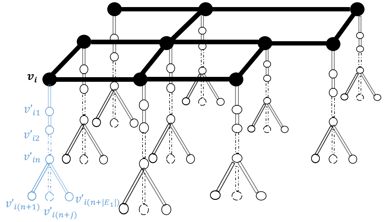
Figure 2: The graph constructed from the sensing graph in Fig. 1.

In the following proposition, we show that an optimal solution to the mobile crowdsensing setting can infer an optimal solution to the static setting, which further reveals the NP-hardness for our mobile crowdsensing setting. We prove Proposition III.3 in Appendix -A.

Proposition III.3.

An optimal solution to the mobile crowdsensing setting with input $I_{\rm e}=(G^{\prime}_{1},G_{2})$ $\iff$ an optimal solution to the static crowdsensing setting with input $I_{\rm o}=(G_{1},G_{2})$.

With Proposition III.3, the NP-hardness for the mobile crowdsensing crowdsensing setting holds readily. ∎

In the following Section IV, we focus on algorithm design in the static crowdsensing setting as a warm-up, built upon which we will further advance our approximation algorithms for mobile crowdsensing setting later in Section V.

IV Greedy Algorithm for Static Crowdsensing

To solve the static crowdsensing setting of the problem (6), we present Algorithm 1, referred to as GUS. The key idea of GUS is to myopically select a user to maximize the marginal welfare brought to the system at each time.

Algorithm 1 Greedy-User-Select (GUS)

Input: $G_{1}=(V,E_{1})$, $G_{2}=(V,E_{2})$ and $k$.
Output: $S_{k}=\{s_{1},...,s_{k}\}$.

1:  for $s_{i}=s_{1},...,s_{k}$ do

2:     Select $s_{i}\leftarrow\arg\max\limits_{v_{x}\in V}\left\{{\Phi}(S_{i-1}\cup\{v_{x}\})-{\Phi}(S_{i-1})\right\}$.

3:  end for

Despite its simple looking in step 2, running Algorithm 1 still requires inputting the precise value of each $\Phi(S_{i})$ directly from the objective function (5). In fact, the computation method for $\Phi(S_{i})$ determines the time complexity of Algorithm 1. Benefits from our meticulous characterizations of the interaction effects between social network $G_{2}$ and sensing network $G_{1}$, we manage to find an efficient approach to computing $\Phi(S_{i})$ via translating the involved social PoI sharing process into matric computation. Of independent interest, our approach to computing $\Phi(S_{i})$ also enables us to adapt our algorithms readily to a range of extensions, as we discuss later at the end of this section.

IV-A Tractable Approach to Computing $\Phi(S_{i})$ in (5)

We start off by considering the basic case of static crowdensing without utility preference. Then, we will extend the approach to a typical case of static crowdsensing with utility preference.

IV-A1 Static Crowdsensing without Utilization Preference

We first look at the initial condition where no user is selected to broadcast its PoI yet, i.e., $\Phi(\varnothing)$. The reason for starting from $\Phi(\varnothing)$ is twofold: first, it relates to the first and important selected user $s_{1}$ in an initial step; second, it serves as a building block for further computing each $\Phi(S_{i})$ for $i\in\{2,...,k\}$. Our approach to $\Phi(\varnothing)$, as summarized in its pseudocode in Algorithm 2, consists of the following four steps where we use bold symbols to tell vectors.

Step 1. Construct sensing matrix $\textbf{A}=(a_{i,j})_{1\leq i,j\leq m}$ from the sensing graph $G_{1}$ as follows: for each entry $a_{i,j}$ (i.e., the entry in the $i$-th row and the $j$-th column of the matrix A), its value is determined as

$$a_{i,j}=\left\{\begin{matrix}1,&{\rm if\;}i\neq j{\rm\;and\;}(v_{i},v_{j})\in E_{1},\\ 0,&{\rm otherwise}.\end{matrix}\right.$$ (11)

Here, an entry is set as one only when the corresponding edge exists in the graph. Entries in the main diagonal of matrix $A$ are all set as zero as $G_{1}$ does not have a self-loop that connects a node to itself. By replacing the value of $a_{i,j}$ with the corresponding weight of edge $(v_{i},v_{j})\in V$, note that one can easily generalize our approach to the scenario where an edge weight does not have to be uniform.

Step 2. Construct social matrix $\textbf{B}=(b_{i,j})_{1\leq i,j\leq m}$ from given social graph $G_{2}$, where each entry $b_{i,j}$ follows:

$$b_{i,j}=\left\{\begin{matrix}0,&{\rm if\;}i\neq j{\rm\;and\;}(v_{i},v_{j})\notin E_{2},\\ 1,&{\rm otherwise}.\end{matrix}\right.$$ (12)

We set entries on the main diagonal of matrix B as one since each user can access the PoI collected by herself. Note that both $A$ and $B$ are symmetric matrices.

Algorithm 2 Computing $\Phi(\varnothing)$ before any hiring

Input: sensing graph $G_{1}$ and social graph $G_{2}$.

1:  Construct $\textbf{A}=(a_{i,j})_{1\leq i,j\leq m}$, where

$$a_{i,j}=\left\{\begin{matrix}1,&{\rm if\;}i\neq j{\rm\;and\;}(v_{i},v_{j})\in E_{1},\\ 0,&{\rm otherwise}.\end{matrix}\right.$$

2:  Construct $\textbf{B}=(b_{i,j})_{1\leq i,j\leq m}$, where

$$b_{i,j}=\left\{\begin{matrix}0,&{\rm if\;}i\neq j{\rm\;and\;}(v_{i},v_{j})\notin E_{2},\\ 1,&{\rm otherwise}.\end{matrix}\right.$$

3:  Construct $\textbf{C}\triangleq\textbf{AB}$.

4:  for $v_{x}\in V$ do

5:     Construct $M_{\sigma_{x}(B)}$ by selecting those columns and rows in matrix A that correspond to either user $v_{x}$ or $v_{x}$’s friends in set $N_{2}(v_{x})$.

6:     $\phi_{x}(\varnothing)\leftarrow(\sum\limits_{1\leq j\leq m}c_{j,x}-\frac{1}{2}\textbf{e}^{T}_{x}\textbf{M}_{\sigma_{x}(B)}\textbf{e}_{x})$.

7:  end for

8:  Output $\Phi(\varnothing)\leftarrow\frac{1}{m}\sum\limits_{1\leq x\leq m}\phi_{x}(\varnothing)$.

Step 3. Compute the matrix product of A and B, which is denoted as $\textbf{C}=(c_{i,j})_{1\leq i,j,\leq m}$, i.e., $\textbf{C}\triangleq\textbf{AB}.$

For each $v_{x}\in V$, denote $\sigma_{x}(B)$ as the set of indices of zero entries in the $x$-th column of the matrix B. Construct the minor of A by removing from matrix A those rows and columns that are indexed by $\sigma_{x}(B)$, which we denote as $\textbf{M}_{\sigma_{x}(B)}$. Intuitively, $\textbf{M}_{\sigma_{x}(B)}$ is constructed by selecting those columns and rows of matrix A that correspond to either user $v_{x}$ or $v_{x}$’s friends (in set $N_{2}(v_{x})$).

Step 4. Compute $\sum\limits_{1\leq j\leq m}c_{j,x}-\frac{1}{2}\textbf{e}^{T}_{x}\textbf{M}_{\sigma_{x}(B)}\textbf{e}_{x}$, where $\textbf{e}_{x}$ about user $v_{x}$ is an all-one column vector of size $m-|\sigma_{x}(B)|$.

According to the definition (1) of PoI utility function $\phi_{i}(S_{k})$, we can obtain $\phi_{i}(\varnothing)=|E_{1}(\{v_{x}\}\cup N_{1}(v_{x}))|$ from the following lemma which is proved in Appendix -B.

Lemma IV.1.

For each $v_{x}\in V$, the following holds:

$$\phi_{i}(\varnothing)=\sum\limits_{1\leq j\leq m}c_{j,x}-\frac{1}{2}\textbf{e}_{x}^{T}\textbf{M}_{\sigma_{x}(B)}\textbf{e}_{x},$$ (13)

where $\textbf{e}_{x}$ denotes an all-one column vector of size $m-|\sigma_{x}(B)|$.

By applying Lemma IV.1 in (5), one can readily obtain the closed-form of $\Phi(\varnothing)$ as given in the following proposition.

Proposition IV.2.

When no user is selected yet for GUS in Algorithm 1, we have

$$\Phi(\varnothing)=\frac{1}{m}\textbf{e}^{T}\textbf{C}\textbf{e}-\frac{1}{2m}\sum\limits_{v_{x}\in V}\textbf{e}^{T}_{x}\textbf{M}_{\sigma_{x}(B)}\textbf{e}_{x},$$ (14)

in which e denotes an all-one column vector of size $m$.

Proof.

Due to objective function (5) and Lemma 13, we have

$$\begin{split}\Phi(\varnothing)&=\frac{1}{m}\sum\limits_{v_{i}\in V}|E_{1}(\{v_{i}\}\cup N_{1}(v_{i}))|\\ &=\frac{1}{m}\sum\limits_{1\leq i\leq m}\sum\limits_{1\leq j\leq m}c_{j,i}-\frac{1}{m}\sum\limits_{v_{i}\in V}\frac{1}{2}\textbf{e}_{i}^{T}\textbf{M}_{\sigma_{i}(B)}\textbf{e}_{i}\\ &=\frac{1}{m}\textbf{e}^{T}\textbf{C}\textbf{e}-\frac{1}{2m}\sum\limits_{v_{x}\in V}\textbf{e}^{T}_{x}\textbf{M}_{\sigma_{x}(B)}\textbf{e}_{x}.\end{split}$$ (15)

This completes the proof. ∎

Now, we are ready to introduce our approach to computing each $\Phi(S_{i})$ for each $S_{i}\subseteq V$. When the $i$th selected user $s_{i}$ is determined, we suppose w.l.o.g. that the index of $s_{i}$ in set $V$ is $h$, i.e., $s_{i}=v_{h}$. This helps to pin down those entries of the social matrix B that correspond to $s_{i}$, as discussed in the following B-Matrix-Update Step.

B-Matrix-Update Step. $\textbf{B}_{i}$ is updated in the following manner: all the $h$-th row entries of B are updated to 1, which reflects the fact that the PoI information collected by $v_{h}$ will be broadcast to $v_{i}$ as soon as $v_{h}$ is selected. Meanwhile, entries on the $h$th column of B remain, which reflects another fact that $v_{h}$ will not increase her own PoI information size from herself being selected. In this way, $\textbf{B}_{i}$ is obtained as a $m$-by-$m$ matrix that is not symmetric. According to B, the matrix C now is updated as follows. C-Matrix-Update Step. Given a set $S_{i}$ of the first $i$ selected users, matrix C can be updated to $\textbf{C}_{i}$ by:

$$\textbf{C}_{i}=\textbf{AB}_{i}.$$ (16)

Accordingly, $\textbf{M}_{\sigma_{x}(B)}$ is updated to $\textbf{M}_{\sigma_{x}(B)_{i}}$. With $\textbf{C}_{i}$ and $\textbf{M}_{\sigma_{x}(B)_{i}}$ at hand, similar to Proposition IV.2, the following theorem returns $\Phi(S_{i})$ in closed-form. Algorithm 3 summarizes the pseudocode for computing $\Phi(S_{i})$.

Algorithm 3 Computing $\Phi(S_{i})$ for Static crowdsensing without Utility Preference

Input: $G_{1}=(V,E_{1})$, $G_{2}=(V,E_{2})$, $S_{i}=\{s_{1},...,s_{i}\}$.

1:  Construct matrices A and B by Algorithm 2, $\textbf{B}_{0}\leftarrow\textbf{B}$.

2:  for $s_{j}\in(s_{1},...,s_{i})$ do

3:     Find the index of $s_{j}$ in set $V$, denoted as $j^{\prime}$.

4:     Update the $j^{\prime}$-th row entries of matrix $\textbf{B}_{j-1}$ as one.

5:  end for

6:  Compute $\textbf{C}_{i}\leftarrow\textbf{AB}_{i}$.

7:  Output $\Phi(S_{i})\leftarrow\frac{1}{m}\textbf{e}^{T}\textbf{C}_{i}\textbf{e}-\frac{1}{2m}\sum\limits_{v_{x}\in V}\textbf{e}^{T}_{x}\textbf{M}_{\sigma_{x}(B_{i})}\textbf{e}_{x}$, i.e., (17).

Theorem IV.3.

Given the set $S_{i}$ of selected users, we have

$$\Phi(S_{i})=\frac{1}{m}\textbf{e}^{T}(\textbf{C}_{i})\textbf{e}-\frac{1}{2m}\sum\limits_{v_{x}\in V}\textbf{e}^{T}_{x}\textbf{M}_{\sigma_{x}(B_{i})}\textbf{e}_{x},$$ (17)

in which e and $\textbf{e}_{x}$ denote all-ones column vectors with sizes adapted to matrices $\textbf{C}_{i}$ and $\textbf{M}_{\sigma_{x}(B_{i})}$, respectively.

IV-A2 Static Crowdsensing with Utility Preference

Now, we discuss the way to adapt the above tractable approach to the static crowdsensing setting with utility preference. Since each user $v_{i}\in V$ has a unique subset $E_{1}^{(i)}$ of edges of her own interest, we independently compute $\phi_{i}$ for each user $v_{i}$. Here, the sensing matrix is replaced by $\textbf{A}^{i}=(a^{i}_{x,y})_{1\leq x,y\leq m}$, where each entry of $\textbf{A}^{i}$ follows

$$a^{i}_{x,y}=\left\{\begin{matrix}1,&{\rm if\;}x\neq y{\rm\;and\;}(v_{x},v_{y})\in E_{1}^{(i)},\\ 0,&{\rm otherwise}.\end{matrix}\right.$$ (18)

By applying a similar matrix update approach as above in the static crowdsensing setting without utility preference, we obtain Algorithm 4 to compute each $\phi_{i}(S_{i})$ and further each $\Phi_{i}(S_{i})$ in the static crowdsensing setting with utility preference.

Algorithm 4 Computing $\Phi(S_{y})$ for static crowdsensing with utility preference

Input: $G_{1}=(V,E_{1})$, $G_{2}=(V,E_{2})$, $m$, $\{E_{1}^{(1)},...,E_{1}^{(m)}\}$, $S_{y}=\{s_{1},...,s_{y}\}$.

1:  Construct $\textbf{B}_{0}=(b_{i,j})_{1\leq i,j\leq m}$, where

$$b_{i,j}=\left\{\begin{matrix}0,&{\rm if\;}i\neq j{\rm\;and\;}(v_{i},v_{j})\notin E_{2}\\ 1,&{\rm otherwise}\end{matrix}\right.$$

2:  for $s_{i}\in(s_{1},...,s_{y})$ do

3:     Find the index of $s_{i}$ in set $V$, denoted as $i^{\prime}$.

4:     Construct matrix $\textbf{B}_{i}$ by updating in $\textbf{B}_{i-1}$ all the $i^{\prime}$-th row entries to one.

5:  end for

6:  for $v_{x}\in V$ do

7:     Construct $\textbf{A}^{x}=(a^{x}_{i,j})_{1\leq i,j\leq m}$,

$$a^{x}_{i,j}=\left\{\begin{matrix}1,&{\rm if\;}i\neq j{\rm\;and\;}(v_{i},v_{j})\in E_{1}^{(x)}\\ 0,&{\rm otherwise}\end{matrix}\right.$$

8:     Compute $\textbf{C}^{x}\triangleq\textbf{A}^{x}\textbf{B}_{y}$.

9:     Compute $\textbf{M}_{\sigma_{x}(B^{x})}$.

10:     $\phi_{x}(S_{y})\leftarrow(\sum\limits_{1\leq j\leq m}c^{i}_{j,x}-\frac{1}{2}\textbf{e}^{T}_{x}\textbf{M}_{\sigma_{x}(B)}\textbf{e}_{x})$.

11:  end for

12:  Output $\Phi(S_{y})\leftarrow\frac{1}{m}\sum\limits_{1\leq x\leq m}\phi_{x}(S_{y})$.

Remark IV.4 (On our computing approach).

Our computing approach accommodates various generalized scenarios, e.g.,

• Sensing-graph adaptive. If the weight of PoI information varies across different edges, we modify the corresponding entry in our sensing graph matrix A to reflect the specific weight. If the sensing graph $G_{1}$ contains loops (i.e., self-connections), we update the corresponding diagonal entries in our sensing matrix A to one.

• Social-information-dissemination adaptive. To accommodate the desired number of hops for information dissemination in the social graph, we have the flexibility to adjust the social connections of specific users by modifying the corresponding entries in their social matrix $B$.

In the following, we discuss the approximation that can be guaranteed by our Algorithm 1 with its subroutine Algorithms 2, 3, 4 (for computing each $\Phi(S_{i})$).

IV-B Approximation Result

To present our approximation results for Algorithm 1, we need to introduce a desired property for set functions (including our function $\Phi(S_{i})$), which is the submodularity. Any set function $f(\cdot)$, which is defined over subsets of a given finite set, is called submodular if

$$f(S\cup\{v\})-f(S)\geq f(V\cup\{v\})-f(V),$$

holds for all elements $v$ and pairs of sets $S\subseteq V$. As a critical step in establishing our approximation results, we show in the following lemma that our function $\Phi(V)$ in (5) meets some desired properties including submodularity.

Lemma IV.5.

Given any sensing graph $G_{1}=(V\cup V^{\prime},E_{1})$ and social graph $G_{2}(V,E_{2})$, $\Phi(S)$ is non-decreasing in subset $S\subseteq V$ and submodular.

Proof.

For any two node subsets $V^{\prime},V^{\prime\prime}\subseteq V$ and any subset $E_{1}^{(i)}\subseteq E_{1}$, we observe

$$|E_{i}(V^{\prime}\cup V^{\prime\prime})|=|E_{i}(V^{\prime})|+|E_{i}(V^{\prime\prime})|-|E_{i}(V^{\prime}\cap V^{\prime\prime})|,$$ (19)

and

$$\begin{split}&|E_{1}^{(i)}\cap E_{i}(V^{\prime}\cup V^{\prime\prime})|+|E_{1}^{(i)}\cap E_{i}(V^{\prime}\cap V^{\prime\prime})|\\ &=|E_{1}^{(i)}\cap E_{i}(V^{\prime})|+|E_{1}^{(i)}\cap E_{i}(V^{\prime\prime})|.\end{split}$$ (20)

In the following two cases, we prove that function $\Phi(S_{i})$ in (5) achieves monotonicity and submodularity, respectively.

Result 1. (monotonicity of $\phi_{i}(S)$)

For an arbitrary subset $S\subseteq V$ and an arbitrary element $v\in V-S$, the following holds readily due to Equation (1):

$$\begin{split}&\phi_{i}(S\cup\{v\})\\ &=|E_{1}(\{v_{i}\}\cup N_{2}(v_{i})\cup S\cup\{v\})|\\ &=|E_{1}(\{v_{i}\}\cup N_{2}(v_{i})\cup S)\cup E_{1}(\{v\})|\\ &\geq|E_{1}(\{v_{i}\}\cup N_{2}(v_{i})\cup S)|=\phi_{i}(S),\end{split}$$ (21)

for any user $v_{i}\in V$, telling that $\phi_{i}(S)$ is non-decreasing over subsets $S\subseteq V$. Further by Equation (5), we know $\Phi_{i}(S)$ is non-decreasing in $S\subseteq V$.

Result 2. (submodularity of $\phi_{i}(\cdot)$)

For any two subsets $S_{1},S_{2}\subseteq V$ with $S_{1}\subseteq S_{2}$, and an element $v\in V$, we have

$$\begin{split}&\phi_{i}(S_{2}\cup\{v\})-\phi(S_{2})\\ &=|E_{1}(\{v_{i}\}\cup N_{2}(v_{i})\cup S_{2}\cup\{v\})|-|E_{1}(\{v_{i}\}\cup N_{2}(v_{i})\cup S_{2})|\\ &=|E_{1}(\{v\})|-|E_{1}(\{v_{i}\}\cup N_{2}(v_{i})\cup S_{2})\cap\{v\})|\\ &\leq|E_{1}(\{v\})|-|E_{1}(\{v_{i}\}\cup N_{2}(v_{i})\cup S_{1})\cap\{v\})|\\ &=\phi_{i}(S_{1}\cup\{v\})-\phi_{i}(S_{1}),\end{split}$$

where the first equation is due to Equation (1), the first inequality holds since $S_{1}\subseteq S_{2}$, and the second and the last equations hold by (19). Therefore, each $\phi_{i}(\cdot)$ is submodular over subsets of $V$. Further by Equation (5), we know $\Phi(\cdot)$ is submodular as well.

Due to (20) and the fact that $E_{1}^{(i)}$ is a fixed edge subset, each $\phi_{i}(\cdot)$ meets the monotonicity and submodularity in the static crowdsensing setting. Further, the summation over every $\phi_{i}(\cdot)$, which is $\Phi(\cdot)$ is submodular and non-decreasing as well. ∎

Inspired by [31], the following lemma provides another useful foundation for establishing our approximation results.

Lemma IV.6.

For maximization problems that select $k$ elements one at a time, if the objective function $f(\cdot)$ on subsets of a finite set $V$, is submodular, non-decreasing, and $f(\varnothing)=0$, we can obtain a solution with performance value at least $1-(\frac{k-1}{k})^{k}$ fraction of the optimal value, which is done by selecting an element that provides the largest marginal increase in the function value.

In light of Lemmas IV.5 and IV.6, we can derive our approximation guarantee as in the following theorem.

Theorem IV.7.

For the static crowdsensing setting of the social-enhanced PoI sharing problem (6), Algorithm 1 with its subroutine Algorithms 2, 3, 4 guarantees an approximation $1-\frac{m-2}{m}(\frac{k-1}{k})^{k}$ of the optimum. It runs in polynomial-time with complexity $O(k(m-k)m^{2.2372})$.

Proof.

Benefits from a recent matrix multiplication approach [32], our matrix computation-based algorithm can complete each step in its “for-loop” in $O(m^{2.372})$-time. In total, our Algorithm 1 runs in $O(k(m-k)m^{2.2372})$-time.

To show the approximation guaranteed by Algorithm 1, we introduce a new function $\widetilde{\Phi}(S_{k})$ as follows:

$$\widetilde{\Phi}(S_{k})=\Phi(S_{k})-\Phi(\varnothing),$$ (22)

where $\Phi(\varnothing)$ and $\Phi(S_{k})$ are returned by subroutine Algorithms 2 and 3, respectively.

By Lemma IV.5, one can easily check that $\widetilde{\Phi}(S_{k})$ is non-decreasing, sub-modular and $\widetilde{\Phi}(\varnothing)=0$. Moreover, it follows

$$\begin{split}&\arg\max\limits_{v_{x}\in V}\left\{\widetilde{\Phi}(S_{i-1}\cup\{s_{x}\})-\widetilde{\Phi}(S_{i-1})\right\}\\ &=\arg\max\limits_{v_{x}\in V}\left\{{\Phi}(S_{i-1}\cup\{s_{x}\})-{\Phi}(S_{i-1})\right\}.\end{split}$$ (23)

In the “for-loop” part of Algorithm 1, by replacing function $\Phi(\cdot)$ with $\widetilde{\Phi}(\cdot)$, the following holds by Lemma IV.6:

$$\widetilde{\Phi}(S_{k})\geq[1-(\frac{k-1}{k})^{k}]\cdot\widetilde{\Phi}(S_{k}^{*}),$$ (24)

which implies

$$\Phi(S_{k})\geq[1-(\frac{k-1}{k})^{k}]\cdot\Phi(S_{k}^{*})+(\frac{k-1}{k})^{k}\Phi(\varnothing),$$ (25)

due to the fact that $\Phi(\varnothing)$ remains unchanged regardless of the specific sets $S_{k}$ and $S_{k}^{*}$.

Hence, we obtain from (7) that

$$\begin{split}\rho\geq[1-(\frac{k-1}{k})^{k}]+(\frac{k-1}{k})^{k}\frac{\Phi(\varnothing)}{\Phi(S_{k}^{*})}.\end{split}$$ (26)

To reveal our approximation guarantee, we need further bound $\frac{\Phi(\varnothing)}{\Phi(S_{k}^{*})}$ in (26). Thereby, we further discuss two cases.

Case 1. In the setting of static crowdsensing without utility preference, we notice, on the one hand, that $|E_{1}(V)|$ is a natural upper bound on $|\Phi(S_{k}^{*})|$, i.e.,

$$|\Phi(S_{k}^{*})|\leq|E_{1}(V)|.$$ (27)

On the other hand,

$$\begin{split}\Phi(\varnothing)&=\frac{1}{m}\sum\limits_{v_{i}\in V}|E_{1}(\{v_{i}\}\cup N_{2}(v_{i}))|\\ &\geq\frac{1}{m}\sum\limits_{v_{i}\in V}|E_{1}(\{v_{i}\})|=\frac{2|E_{1}|}{m},\end{split}$$ (28)

where the first equation is due to Equations (1) and (5), the first inequality holds by the monotonicity of the function $\Phi(\cdot)$, and the second equation holds since each edge $(v_{x},v_{y})\in V$ is counted twice in the summation $|\sum\limits_{v_{i}\in V}|E_{1}({v_{i}})|$ because it is considered separately for $E_{1}({v_{x}})$ and $E_{1}({v_{y}})$. Plugging Inequalities (27) and (28) in Inequality (26), yields

$$\begin{split}\rho&\geq 1-(\frac{k-1}{k})^{k}+(\frac{k-1}{k})^{k}\frac{\frac{2|E_{1}|}{m}}{|E_{1}|}=1-\frac{m-2}{m}(\frac{k-1}{k})^{k}.\end{split}$$

Case 2. For static crowdsensing with utility preference, we have

$$\begin{split}\frac{\Phi(\varnothing)}{\Phi(S_{k}^{*})}&\geq\frac{\frac{1}{m}\sum\limits_{v_{i}\in V}|E_{1}^{(i)}\cap E_{1}(\{v_{i}\}\cup N_{2}(v_{i}))|}{\frac{1}{m}\sum\limits_{v_{i}\in V}|E_{1}^{(i)}|}\\ &\geq\frac{\frac{1}{m}\sum\limits_{v_{i}\in V}|E_{1}(\{v_{i}\})|}{\frac{1}{m}\sum\limits_{v_{i}\in V}|E_{1}^{(i)}|}\geq\frac{2}{m},\end{split}$$ (29)

where the first inequality holds because ${\frac{1}{m}\sum\limits_{v_{i}\in V}|E_{1}^{(i)}|}$ is a natural upper bound on the optimal solution in this setting, and the last two inequalities hold by $E_{1}^{(i)}\subseteq E_{1}$.

Finally, we have by plugging (29) in (26) that

$$\rho\geq 1-\frac{m-2}{m}(\frac{k-1}{k})^{k}.$$ (30)

Cases 1-2 conclude the proof. ∎

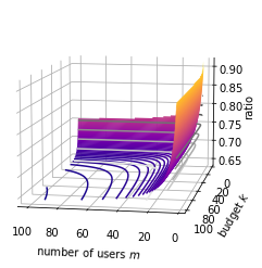
Figure 3: Visualization of the approximation guarantee for Algorithm 1 versus budget $k$ and the number $m$ of selected users.

We note that the theoretical guarantee for our Algorithm 1, as presented above in Theorem IV.7, exhibits a monotonically decreasing trend as $k$ or $m$ increases. Fig. 3 numerically depicts an overview of our theoretical guarantee versus the budget $k$ and the number $m$ of selected users, from which we can tell that our Algorithm 1 particularly fits small-size networks or low budgets. Even in a dense network or with a large budget, Fig. 3 shows that Algorithm 1 still guarantees at least a ($1-\frac{1}{e}$) proportion of the optimal welfare.

V New Augmentation-Adaptive Algorithms for Mobile Crowdsensing

In this section, we circumvent the routing intricacies in the mobile crowdsensing setting by transforming it into an optimization alternative, which allows us to analyze the problem within the framework established for our fundamental setting in Section IV. Before introducing our problem transformation, we recall in (3) that the path $p_{j}$ recommended to each selected user $s_{j}\in S_{k}$ should admit:

• $p_{j}$ starts from the location of the user node $s_{j}$, and

• the length of $P_{j}$ equals $n$, i.e., $|p_{j}|=n$.

Inspired by these two characters of a recommended path, we transform the problem of the mobile crowdsensing setting to a new Problem (31)-(33), which is via the following steps:

• For each user $v_{i}\in V$, we identify all possible paths starting from the location $v_{i}$ and having an overall length $n$ of edges in $G_{1}$. Then, we collect all those paths identified and store them in path set $\mathcal{P}$. Note that, by applying Floyd-Warshall Algorithm [33], $\mathcal{P}$ can be found in $O((|V^{\prime}|+m)^{n})$-time.

• Find a subset $P\subseteq\mathcal{P}$ of $k$ paths from $k$ distinct start nodes, such that $\sum\limits_{v_{i}\in V}|E_{1}(\{v_{i}\}\cup N_{2}(v_{i})\cup N_{1}(P))|$ (i.e., the sum of objective (4) among users) is maximized.

• As such, our problem is equivalently converted from (6) to the following Problem (31)-(33):

  $$\max\limits_{P\subseteq\mathcal{P}} \frac{1}{m}\sum\limits_{v_{i}\in V}|E_{1}(\{v_{i}\}\cup N_{2}(v_{i})\cup N_{1}(P))|$$ (31)

  $${\rm s.t.} \mathcal{P}\triangleq\{p\subseteq E_{1}\big{|}p{\rm\;is\;from\;a\;user\;},|p|=n\},$$ (33)

  $$|P|=k.$$

Notice that the search space $\mathcal{P}$ of the above Problem (31)-(33) may include multiple paths that start from the same user node. This motivates us to further consider the following question: can we achieve more welfare efficiency when each user node has multiple users instead? Accordingly, we look at an advanced resource-augmented version of the problem, where the high-level insight is that: when the algorithm with an acceptable augmentation outperforms significantly the original solution, it makes sense to invest to invite more users to join at each sensing node [34, 35, 36].

For our social-enhanced PoI sharing problem, we introduce a new resource augmentation scheme as follows: given an input instance $I=(G_{1},G_{2})$ of two graphs for the mobile crowdsensing setting, we create an augmented instance $I_{g}$ to allow each user node of $G_{1}$ to have $g\geq 1$ users. Accordingly, the approximation ratio with augmentation factor $g$ tells the worst-case ratio of an approximation algorithm’s welfare on $I_{g}$ over an optimal solution’s welfare on original $I$, i.e.,

$$\rho=\inf\limits_{I}\frac{\Phi(P_{k}(I_{g}))}{\Phi(P_{k}^{*}(I))}.$$ (34)

Based on an augmented instance $I_{g}$, we propose a new augmentation-adaptive approach to fit any $g$ in Algorithm 5 which we name as GPS. In general, the GPS algorithm first constructs the search space $\mathcal{P}$, and then dynamically selects a path that brings the largest marginal welfare, subject to the constraint that the number of paths originating from a user node does not exceed the augmentation factor $g$.

Algorithm 5 Greedy-Path-Select (GPS)

Input: $G_{1}=(V,E_{1})$, $G_{2}=(V,E_{2})$, $n$, $k$ and $g$
Output: $P=\{p_{1},...,p_{k}\}$

1:  Construct $\mathcal{P}$ by the Floyd-Warshall Algorithm [33], and set $P\leftarrow\varnothing$.

2:  for $i\in[k]$ do

3:     Select $p_{i}\leftarrow\arg\max\limits_{p\in\mathcal{P}}\left\{{\Phi}(P\cup\{p_{i}\})-{\Phi}(P)\right\}$.

4:     $P\leftarrow P\cup\{p_{i}\}$.

5:     Find in $P$ all those paths that start with the same user node as $p_{i}$, denoted as $P_{i}$.

6:     if $|P_{i}|=g$ then

7:        Find in $\mathcal{P}$ all those paths that start with the same user node as $p_{i}$, denoted as $\mathcal{P}_{i}$.

8:        $\mathcal{P}\leftarrow\mathcal{P}-\mathcal{P}_{i}$.

9:     end if

10:  end for

Time-complexity Analysis. Before showing the welfare performance of our Algorithm 5, we first discuss its time complexity. In Algorithm 5, the running time of each iteration of the “for-loop” is dominated by Step 3 for selecting path $p_{i}$, which highly depends on $\Phi$. To this end, we first discuss our approach to computing $\Phi$ which is refined from Algorithm 3. Since node-set sizes between graphs $G_{1}$ and $G_{2}$ are not guaranteed to be the same in the mobile crowdsensing setting, we suppose for ease of exposition that the first $m$ indices of nodes in $G_{1}(V\cup V^{\prime},E_{1})$ correspond to user nodes in $V$. Denote $\varpi\triangleq|V\cup V^{\prime}|$ as the number of nodes in the sensing graph $G_{1}$. Then, the social matrix in our previous Algorithm 3 is updated to the following $\varpi\times\varpi$ matrix $\textbf{B}^{i}=(b^{i}_{x,y})_{1\leq x,y\leq m}$, where

$$b^{i}_{x,y}=\left\{\begin{matrix}1,&{\rm if\;}x=y{\rm\;or\;}(v_{x},v_{y})\in E_{2}^{(i)},\\ 0,&{\rm otherwise}.\end{matrix}\right.$$

Since each selected user $v_{i}$ will collect PoI information from roads that are incident to at least one node on the path $p_{i}$ now, we update in the “for-loop” of Algorithm 3 by adding an inner-for-loop to update in matrix $\textbf{B}_{j-1}$ those row entries (corresponding to nodes in $p_{i}$) to one. The following theorem summarizes our results for the mobile crowdsensing setting.

Theorem V.1.

For the mobile crowdsensing setting of the social-enhanced PoI sharing problem, Algorithm 5 (GPS) with augmentation factor $g\in\{1,...,k\}$ guarantees an approximation ratio of at least

$$\frac{g}{k}[1-\frac{\varpi-2}{\varpi}(\frac{k-1}{k})^{k}],$$

where $\varpi=|V\cup V^{\prime}|$ denotes the node size of $G_{1}$, and runs in $O(k(\varpi^{n}-k)\varpi^{2.372})$-time.

Proof.

Regarding the Time complexity, note that the size of the path set $\mathcal{P}$ is no more than $\varpi^{n}$, where $\varpi=|V\cup V^{\prime}|$. Due to our matrix multiplication approach in Theorem IV.3, we can obtain each $\Phi(S_{i})$ in $O(\varpi^{2.372})$-time. To compute each $p_{i}$, our Algorithm 5’s Step 3 takes at most ($\varpi^{n}-i+1$) iterations in which each iteration takes $O(\varpi^{2.372})$-time. Thereby, the whole “for-loop” of Algorithm 5 runs in $O(k(\varpi^{n}-k)\varpi^{2.372})$-time. Moreover, the initial step for constructing $\mathcal{P}$ can be done by the Floyd-Warshall Algorithm [33] in $O((|V^{\prime}|+m)^{n})$-time, which is smaller than $O(k(\varpi^{n}-k)\varpi^{2.372})$. In total, we know that Algorithm 5 runs in $O(k(\varpi^{n}-k)\varpi^{2.372})$-time.

Similar to the proof of Lemma IV.5, it is easy to check that our new objective (31) for the mobile crowdsensing setting remains monotonicity and submodularity. Given an instance $I=(G_{1},G_{2})$ of our problem, denote $I_{x}$ as the augmented instance with factor $g=x$. The only difference between $I_{x}$ and $I$ is that each user node of the sensing graph $G_{1}$ in instance $I_{x}$ contains exactly $x$ identical users instead of exactly one in the original instance $I$. Denote $P$ and $P^{*}$ as the set of paths that are generated by our Algorithm 5 with augmentation $g=x$ and an optimal solution, respectively.

Before showing our approximation result, we note a feature of our Algorithm 5, which possibly narrows the search space by the “if-else” of Algorithm 5 in some of its selection iterations. This feature makes the submodularity result in Lemma IV.6 not be applied straightforwardly in deriving the approximation guarantee of Algorithm 5. In other words, the result in Lemma IV.6 could be applied only when the search space does not change (i.e., the “if-else” branches of Algorithm 5 is reduced). As such, our Algorithm 5 with augmentation factor $g=k$ does not change its search space. In the following, we discuss two cases.

VI Concluding Remarks

This work studies the social-enhanced PoI sharing problem, which integrates two independent urban sensing and online social networks into a unified objective for maximizing the average amount of useful PoI information to users. As a theoretical foundation, we prove that such a problem is NP-hard and also renders existing approximation solutions not viable. By analyzing the interplay effects between the sensing and social networks, we successfully transform the involved PoI-sharing process across two networks to matrix computations for deriving a closed-form objective, which not only enables our later approximation analysis but also allows for our subsequent solutions’ various adaptabilities in further social information dissemination, varied PoI weight assignments, etc. In a fundamental setting where users collect PoI information only within the vicinity of their current locations, we leverage some desired properties observed in the objective function to present a polynomial-time $1-\frac{m-2}{m}(\frac{k-1}{k})^{k}$-approximate algorithm. When allowing each selected user to move around and sense more PoI information to share, we apply a new resource-augmented technique and propose an augmentation-adaptive algorithm that achieves bounded approximations of the optimum. These approximation bounds range from $\frac{1}{k}(1-\frac{1}{e})$ to $1-\frac{1}{e}>0.632$ when the augmentation factors range from one to the designated budget $k$. In addition, our theoretical results are corroborated by our simulation findings using both synthetic and real-world datasets.

Songhua Li received the Ph.D. degree from the Department of Computer Science, City University of Hong Kong, in 2022. He is now a postdoctoral research fellow at the Singapore University of Technology and Design (SUTD). His research interests include approximation and online algorithm design and analysis, combinatorial optimization, and algorithmic mechanism design in the context of sharing economy networks.

Lingjie Duan (Senior Member, IEEE) received the Ph.D. degree from The Chinese University of Hong Kong in 2012. He is currently an Associate Professor of Engineering Systems and Design at the Singapore University of Technology and Design (SUTD). In 2011, he was a Visiting Scholar at the University of California at Berkeley, Berkeley, CA, USA. His research interests include network economics and game theory, network security and privacy, energy harvesting wireless communications, and mobile crowdsourcing. He is an Editor of IEEE Transactions on Wireless Communications, and also an associate editor of IEEE Transactions on Mobile Computing. He was an Editor of IEEE Communications Surveys and Tutorials. He also served as a Guest Editor of the IEEE Journal on Selected Areas in Communications Special Issue on Human-in-the-Loop Mobile Networks, as well as IEEE Wireless Communications Magazine. He received the SUTD Excellence in Research Award in 2016 and the 10th IEEE ComSoc AsiaPacific Outstanding Young Researcher Award in 2015.

-A Omitted Proof in Proposition III.3

Proof of Proposition III.3.

Note that only nodes in $V$ could there exist users stand-by for collecting data. For a selected user, say $v_{i}\in V$, we consider the following $n$-hop-forward move in the mobile crowdsensing setting:

$$(v_{i},v^{\prime}_{i1},v^{\prime}_{i2},...,v^{\prime}_{in}).$$ (35)

After the above $n$-hop-forward move, $v_{i}$ could collect PoI information from both edges $E_{1}$ that are incident to $v_{i}$ and those edges in $E^{\prime}_{i}$ (which only correspond to $v_{i}$ herself). We notice the following:

$$|E^{\prime}_{i}|=n+|E_{1}|>|E_{1}|.$$ (36)

This implies that the best $n$-hop-forward move for $v_{i}$, in terms of increasing her contributed data to the system, should follow the path in (35). Hence, regardless of which $k$ users are selected, (4) consistently indicates that

$$\phi_{i}(S_{k})=|E_{1}(\{v_{i}\}\cup N_{2}(v_{i})\cup S_{k}|+k\cdot(n+|E_{1}|).$$ (37)

Further, by (5), we have

$$\Phi(S_{k})=\underbrace{\frac{nk+k|E_{1}|}{m}}_{\rm constant}+\underbrace{\frac{1}{m}\sum\limits_{v_{i}\in V}|E_{1}(\{v_{i}\}\cup N_{2}(v_{i})\cup S_{k})|}_{\rm panoramic\;objective}.$$ (38)

This proves Proposition III.3. ∎

-B Omitted Proof in Lemma IV.1

Proof.

We note the following equations, in which the first equation is due to the matrix multiplication principle and the second equation holds by reorganizing the right-hand-side terms of the first equation.

$$\sum\limits_{1\leq j\leq m}c_{j,x} = \underbrace{(a_{1,1}b_{1,x}+a_{1,2}b_{2,x}+...+a_{1,m}b_{m,x})}_{i.e.,c_{1,x}}$$ (39)

$$+\underbrace{(a_{2,1}b_{1,x}+a_{2,2}b_{2,x}+...+a_{2,m}b_{m,x})}_{i.e.,c_{2,x}}$$

$$\;\;\vdots$$

$$+\underbrace{(a_{m,1}b_{1,x}+a_{m,2}b_{2,x}+...+a_{m,m}b_{m,x})}_{i.e.,c_{m,x}}$$

$$= \underbrace{a_{1,1}b_{1,x}+a_{2,1}b_{1,x}+...+a_{m,1}b_{1,x}}_{i.e.,b_{1,x}\cdot(\sum_{1\leq j\leq m}a_{j,t})}$$

$$+\underbrace{(a_{1,2}b_{2,x}+a_{2,2}b_{2,x}+...+a_{m,2}b_{2,x})}_{i.e.,b_{2,x}\cdot(\sum_{1\leq j\leq m}a_{j,t})}$$

$$\;\;\vdots$$

$$+\underbrace{(a_{1,m}b_{m,x}+a_{2,m}b_{m,x}+...+a_{m,m}b_{m,x})}_{i.e.,b_{m,x}\cdot(\sum_{1\leq j\leq m}a_{j,t})}$$

$$= \sum\limits_{1\leq t\leq m}b_{t,x}\cdot(\sum_{1\leq j\leq m}a_{j,t}).$$

Since A is a symmetric matrix, see Equation (11), $\sum_{1\leq j\leq m}a_{j,t}$ indicates the number of edges that are incident to user $v_{t}\in V$. Due to Equation (12), we know that $b_{t,x}$ equals one only when user $v_{t}$ is either exactly $v_{x}$ or a neighbor of $v_{x}$. In other words, $\sum\limits_{1\leq t\leq m}b_{t,x}\cdot(\sum_{1\leq j\leq m}a_{j,t})$ counts the number of edges that are incident to nodes in $\{v_{x}\}\cup N_{2}{v_{x}}$ independently and sums up those counts together. The following two propositions support our result.

Proposition .1.

$\sum\limits_{1\leq t\leq m}b_{t,x}\cdot(\sum\limits_{1\leq j\leq m}a_{j,t})$ counts an edge that connects two nodes of $\{v_{x}\}\cup N_{2}(v_{x})$ two times, counts an edge that connects a node of $\{v_{x}\}\cup N_{2}(v_{x})$ and a node of $V-\{v_{x}\}\cup N_{2}(v_{x})$ one time, and counts an edge that connects two nodes of $V-\{v_{x}\}\cup N_{2}(v_{x})$ zero time.

Proof.

Note that each edge $(v_{i},v_{j})$ could be counted at most twice by counting edges that are incident to the two end nodes $v_{i}$ and $v_{j}$, respectively. Due to our model, an edge that connects two nodes in $V-\{v_{x}\}\cup N_{2}(v_{x})$ is available to $v_{x}$, and hence, could not be counted in $\sum\limits_{1\leq j\leq m}c_{j,x}$. An edge that connects a node in $\{v_{x}\}\cup N_{2}(v_{x})$ and a node in $V-\{v_{x}\}\cup N_{2}(v_{x})$ is counted only once when counting the edges that are incident to the node in $\{v_{x}\}\cup N_{2}(v_{x})$. An edge that connects to two nodes in $\{v_{x}\}\cup N_{2}(v_{x})$ will be counted twice when independently counting edges that are incident to the two nodes. ∎

Proposition .2.

$\frac{1}{2}\textbf{e}_{x}^{T}\textbf{M}_{\sigma_{x}(B)}\textbf{e}_{x}$ indicates the number of different edges counted in $\sum\limits_{1\leq t\leq m}b_{t,x}\cdot(\sum\limits_{1\leq j\leq m}a_{j,t})$ that connect two nodes in $\{v_{x}\}\cup N_{2}(v_{x})$.

Proof.

For each user, say $v_{x}\in V$, her corresponding matrix $\textbf{M}_{\sigma_{x}(B)}$ consists of those rows and columns of the matrix A whose indices in matrix C equal 1. In other words, $\textbf{M}_{\sigma_{x}(B)}$ reflects the road connection in $G_{1}$ among (users) nodes of $\{v_{x}\}\cup N_{2}(v_{x})$ (which includes $v_{x}$ and her neighbors in graph $G_{2}$). Thus, an entry $(i,j)$ of $\textbf{M}_{\sigma_{x}(B)}$ equals one if and only if $v_{i}$ and $v_{j}$ are in the intersection $\{v_{x}\}\cup N_{2}(v_{x})$ and are connected in graph $G_{1}$. Since A is a symmetric matrix, its minor matrix $\textbf{M}_{\sigma_{x}(B)}$ is also symmetric. Hence, $\textbf{e}_{x}^{T}\textbf{M}_{\sigma_{x}(B)}\textbf{e}_{x}$, which is the sum of all entries of $\textbf{M}_{\sigma_{x}(B)}$, doubles the number of different edges that connect two nodes in $\{v_{x}\}\cup N_{2}(v_{x})$. This completes the proof. ∎

Therefore, Lemma IV.1 follows accordingly. ∎

-C Missed Time Complexity Analysis in Theorem IV.7

To start with, we discuss the time complexities of our algorithms. It is clear that the time complexity of Algorithm 1 largely depends on the single step in its “for-loop”, which is further determined by Algorithms 2 and 3. Before discussing the specific time complexities of our algorithms in different settings, we note that a very recent work [32] provides an $O(m^{2.372})$-time matrix multiplication approach for computing two $m\times m$ matrices, which accelerate our approaches as well.

(Running time for static crowdsensing without utility preference). The running time of Algorithm 2 is dominated by the step of matrix multiplication between two $m\times m$ matrices $A$ and $B$, which can be done in $O(m^{2.372})$-time. In Algorithm 3, the initialization step in obtaining $A$ and $B$ can be done in $O(m^{2})$ time by checking each entry of the matrix, the “for-loop” can be done within $O(km)$-time, and $C$ can be got in $O(m^{2.372})$-time, leading to an overall running time of $O(m^{2.372})$. Further, to compute each $s_{i}$, Algorithm 1 needs to check ($m-i+1$) possibility in the single step of the “for-loop” of Algorithm 1. Totally, Algorithm 1 runs in $O(k(m-k)m^{2.372})$-time for the setting of static crowdsensing without utility preference.

(Running time for static crowdsensing with utility preference). Due to Algorithm 4, the part of running time in computing each $\Phi(S_{i})$ is dominated by the second “for-loop”, in which each iteration takes $O(m^{2.372})$-time leading to an overall running time of $O(m^{3.372})$. Further, to compute each $s_{i}$, Algorithm 1 needs to check ($m-i+1$) possibilities in which each takes time $O(m^{3.372})$. In total, Algorithm 1 runs in $O((m-k)km^{3.372})$-time.

-D Omitted Proof in Proposition LABEL:prop_adjusted_nhop_01

Proof of Proposition LABEL:prop_adjusted_nhop_01.

According to the partition rule in Step 4 of Algorithm LABEL:adjusted_greedyhireg_alg, paths in different partitioned classes start from different user nodes, which implies that those paths included in the first “for loop” of Algorithm LABEL:adjusted_greedyhireg_alg start from distinctive user nodes. Further, due to the “if” condition of the second “nested-for-loop”, all the $k$ paths included in $P^{\prime}$ start from $k$ distinctive user nodes. The proposition follows. ∎

-E Omitted Proof in Proposition LABEL:prop_adjusted_nhop_02

Proof of Proposition LABEL:prop_adjusted_nhop_02.

As per our transformed Problem (31)-(33), we know, as mentioned earlier, that different sets of selected paths contribute the same as long as they visit the same set of nodes in the sensing graph $G_{1}$. Denote $V(P^{\prime})$ and $V(P)$ as the set of nodes that are visited by paths in sets $P^{\prime}$ and $P$, respectively. To further show the proposition, it is sufficient to prove

$$V(P^{\prime})\subseteq V(P).$$ (40)

Note that in each path class $C_{i}\in\mathcal{C}$, the first path selected by Algorithm LABEL:adjusted_greedyhireg_alg is also included in the solution $P^{\prime}$ of Adjusted-GPS. For each other path of $p$ in some class $C_{i}\in\mathcal{C}$, we discuss two cases as follows.

Case 1. (There exist nodes in $p$ that do not appear in start nodes of paths included in $P^{\prime}$ at the moment of selection.)

Note that Adjusted-GPS always selects the first one $p({\rm first})$ of such nodes, implying that all those nodes prior to the selected one in $p$ are visited by paths in the current $P^{\prime}$. Further, Adjusted-GPS includes to $P^{\prime}$ a new path that is constructed by extending the sub-path of $p$ starting from node $p({\rm first})$ to $n$-size; this further guarantees that all nodes on $p$ are visited by some paths in $P^{\prime}$. Then, the proposition follows.

Case 2. Each node on $p$ appears as a start nodes of some path included in $P^{\prime}$ at the moment of selection. The proposition follows accordingly. ∎

-F Equivalence Relation between The Optimization and Decision Versions of The Set Cover Problem

In Fig. 4, we present the equivalence relation between the decision version and the well-known optimization version of the set cover problem.

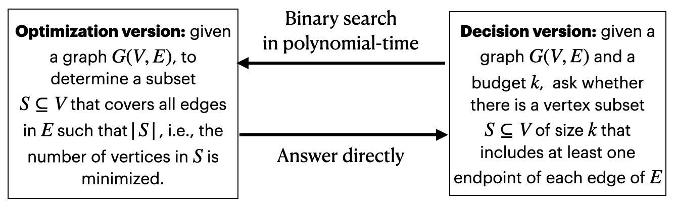
Figure 4: The equivalent relation between the decision and optimization versions of the set cover problem.

References

- [1] A. Capponi, C. Fiandrino, B. Kantarci, L. Foschini, D. Kliazovich, and P. Bouvry, “A survey on mobile crowdsensing systems: Challenges, solutions, and opportunities,” IEEE communications surveys & tutorials, vol. 21, no. 3, pp. 2419–2465, 2019.
- [2] A. Hamrouni, H. Ghazzai, M. Frikha, and Y. Massoud, “A spatial mobile crowdsourcing framework for event reporting,” IEEE transactions on computational social systems, vol. 7, no. 2, pp. 477–491, 2020.
- [3] Flickr. (2023) Find your inspiration. https://www.flickr.com/. Accessed: 2023-05-27.
- [4] TikTok. (2023) Homepage. https://www.tiktok.com/en/. Accessed: 2023-05-27.
- [5] Y. Waitlist. (2023) How can i use yelp waitlist to get in line remotely. https://www.yelp-support.com/article/How-can-I-use-Yelp-Waitlist-to-get-in-line-remotely?l=en_US. Accessed: 2023-05-27.
- [6] G. Waze. (2023) How does waze work. https://support.google.com/waze/answer/6078702?hl=en. Accessed: 2023-05-27.
- [7] Y. Zheng, “Location-based social networks: Users,” in Computing with spatial trajectories. Springer, 2011, pp. 243–276.
- [8] J. Bao, Y. Zheng, D. Wilkie, and M. Mokbel, “Recommendations in location-based social networks: a survey,” GeoInformatica, vol. 19, pp. 525–565, 2015.
- [9] Y. Li, C. A. Courcoubetis, and L. Duan, “Dynamic routing for social information sharing,” IEEE Journal on Selected Areas in Communications, vol. 35, no. 3, pp. 571–585, 2017.
- [10] T. S. Chakravarthy and L. Selvaraj, “Nnpec: Neighborhood node propagation entropy centrality is a unique way to find the influential node in a complex network,” Concurrency and Computation: Practice and Experience, vol. 35, no. 12, p. e7685, 2023.
- [11] M. Cha, A. Mislove, and K. P. Gummadi, “A measurement-driven analysis of information propagation in the flickr social network,” in Proceedings of the 18th international conference on World wide web, 2009, pp. 721–730.
- [12] NCR. (2023) What is tiktok? a guide for restaurant owners. https://www.ncr.com/blogs/restaurants/tiktok-restaurant-owner-guide. Accessed: 2023-05-27.
- [13] S. Fu, H. Li, Y. Liu, H. Pirkkalainen, and M. Salo, “Social media overload, exhaustion, and use discontinuance: Examining the effects of information overload, system feature overload, and social overload,” Information Processing & Management, vol. 57, no. 6, p. 102307, 2020.
- [14] Y.-D. Seo and Y.-S. Cho, “Point of interest recommendations based on the anchoring effect in location-based social network services,” Expert Systems with Applications, vol. 164, p. 114018, 2021.
- [15] D. Kempe, J. Kleinberg, and É. Tardos, “Maximizing the spread of influence through a social network,” in Proceedings of the ninth ACM SIGKDD international conference on Knowledge discovery and data mining, 2003, pp. 137–146.
- [16] S. Li, B. Wang, S. Qian, Y. Sun, X. Yun, and Y. Zhou, “Influence maximization for emergency information diffusion in social internet of vehicles,” IEEE Transactions on Vehicular Technology, vol. 71, no. 8, pp. 8768–8782, 2022.
- [17] D. S. Hochbaum, “Approximation algorithms for the set covering and vertex cover problems,” SIAM Journal on computing, vol. 11, no. 3, pp. 555–556, 1982.
- [18] G. Karakostas, “A better approximation ratio for the vertex cover problem,” ACM Transactions on Algorithms (TALG), vol. 5, no. 4, pp. 1–8, 2009.
- [19] U. Feige, “A threshold of ln n for approximating set cover,” Journal of the ACM (JACM), vol. 45, no. 4, pp. 634–652, 1998.
- [20] N. Christofides, “Worst-case analysis of a new heuristic for the travelling salesman problem,” Carnegie-Mellon Univ Pittsburgh Pa Management Sciences Research Group, Tech. Rep., 1976.
- [21] Y. Livne, D. Atzmon, S. Skyler, E. Boyarski, A. Shapiro, and A. Felner, “Optimally solving the multiple watchman route problem with heuristic search,” in Proceedings of the International Symposium on Combinatorial Search, vol. 15, no. 1, 2022, pp. 302–304.
- [22] J. S. Mitchell, “Approximating watchman routes,” in Proceedings of the twenty-fourth annual ACM-SIAM symposium on Discrete algorithms. SIAM, 2013, pp. 844–855.
- [23] R. K. Ganti, F. Ye, and H. Lei, “Mobile crowdsensing: current state and future challenges,” IEEE communications Magazine, vol. 49, no. 11, pp. 32–39, 2011.
- [24] J. Wang, Y. Wang, D. Zhang, F. Wang, H. Xiong, C. Chen, Q. Lv, and Z. Qiu, “Multi-task allocation in mobile crowd sensing with individual task quality assurance,” IEEE Transactions on Mobile Computing, vol. 17, no. 9, pp. 2101–2113, 2018.
- [25] Y. Lai, Y. Xu, D. Mai, Y. Fan, and F. Yang, “Optimized large-scale road sensing through crowdsourced vehicles,” IEEE Transactions on Intelligent Transportation Systems, vol. 23, no. 4, pp. 3878–3889, 2022.
- [26] H. Wang, H. Shen, W. Ouyang, and X. Cheng, “Exploiting poi-specific geographical influence for point-of-interest recommendation.” in IJCAI, 2018, pp. 3877–3883.
- [27] X. Gong, L. Duan, X. Chen, and J. Zhang, “When social network effect meets congestion effect in wireless networks: Data usage equilibrium and optimal pricing,” IEEE Journal on Selected Areas in Communications, vol. 35, no. 2, pp. 449–462, 2017.
- [28] H. Gao, J. Feng, Y. Xiao, B. Zhang, and W. Wang, “A uav-assisted multi-task allocation method for mobile crowd sensing,” IEEE Transactions on Mobile Computing, 2022.
- [29] D. P. Williamson and D. B. Shmoys, The design of approximation algorithms. Cambridge university press, 2011.
- [30] W. Xu, H. Xie, C. Wang, W. Liang, X. Jia, Z. Xu, P. Zhou, W. Wu, and X. Chen, “An approximation algorithm for the -hop independently submodular maximization problem and its applications,” IEEE/ACM Transactions on Networking, 2022.
- [31] G. L. Nemhauser, L. A. Wolsey, and M. L. Fisher, “An analysis of approximations for maximizing submodular set functions—i,” Mathematical programming, vol. 14, no. 1, pp. 265–294, 1978.
- [32] J. Alman and V. V. Williams, “A refined laser method and faster matrix multiplication,” in Proceedings of the 2021 ACM-SIAM Symposium on Discrete Algorithms (SODA). SIAM, 2021, pp. 522–539.
- [33] T. H. Cormen, C. E. Leiserson, R. L. Rivest, and C. Stein, Introduction to algorithms. MIT press, 2022.
- [34] S. Anand, N. Garg, and A. Kumar, “Resource augmentation for weighted flow-time explained by dual fitting,” in Proceedings of the twenty-third annual ACM-SIAM symposium on Discrete Algorithms. SIAM, 2012, pp. 1228–1241.
- [35] I. Caragiannis, A. Filos-Ratsikas, S. K. S. Frederiksen, K. A. Hansen, and Z. Tan, “Truthful facility assignment with resource augmentation: An exact analysis of serial dictatorship,” Mathematical Programming, pp. 1–30, 2022.
- [36] B. Kalyanasundaram and K. Pruhs, “Speed is as powerful as clairvoyance,” Journal of the ACM (JACM), vol. 47, no. 4, pp. 617–643, 2000.
- [37] GowallaData. (2022) Gowalla dataset. https://snap.stanford.edu/data/loc-gowalla.html. Accessed: 2023-01-13.
- [38] E. Cho, S. A. Myers, and J. Leskovec, “Friendship and mobility: Friendship and mobility: User movement in location-based social networksfriendship and mobility,” in User Movement in Location-Based Social Networks ACM SIGKDD International Conference on Knowledge Discovery and Data Mining (KDD), 2011.
- [39] V. Tripathi and E. Modiano, “Optimizing age of information with correlated sources,” in Proceedings of the Twenty-Third International Symposium on Theory, Algorithmic Foundations, and Protocol Design for Mobile Networks and Mobile Computing, 2022, pp. 41–50.