Generative Bayesian modeling to nowcast the effective reproduction number from line list data with missing symptom onset dates

Abstract

The time-varying effective reproduction number $R_{t}$ is a widely used indicator of transmission dynamics during infectious disease outbreaks. Timely estimates of $R_{t}$ can be obtained from observations close to the original date of infection, such as the date of symptom onset. However, these data often have missing information and are subject to right truncation. Previous methods have addressed these problems independently by first imputing missing onset dates, then adjusting truncated case counts, and finally estimating the effective reproduction number. This stepwise approach makes it difficult to propagate uncertainty and can introduce subtle biases during real-time estimation due to the continued impact of assumptions made in previous steps. In this work, we integrate imputation, truncation adjustment, and $R_{t}$ estimation into a single generative Bayesian model, allowing direct joint inference of case counts and $R_{t}$ from line list data with missing symptom onset dates. We then use this framework to compare the performance of nowcasting approaches with different stepwise and generative components on synthetic line list data for multiple outbreak scenarios and across different epidemic phases. We find that under long reporting delays, intermediate smoothing, as is common practice in stepwise approaches, can bias nowcasts of case counts and $R_{t}$, which is avoided in a joint generative approach due to shared regularization of all model components. On incomplete line list data, a fully generative approach enables the quantification of uncertainty due to missing onset dates without the need for an initial multiple imputation step. In a real-world comparison using hospitalization line list data from the COVID-19 pandemic in Switzerland, we observe the same qualitative differences between approaches. The generative modeling components developed in this work have been integrated and further extended in the R package epinowcast, providing a flexible and interpretable tool for real-time surveillance.

Keywords: nowcasting, effective reproduction number, real-time infectious disease surveillance, missing data, Bayesian generative modeling

Summary

During an infectious disease outbreak, public health authorities require timely indicators of transmission dynamics, such as the effective reproduction number $R_{t}$. Since reporting data are delayed and often incomplete, statistical methods must be employed to obtain real-time estimates of case numbers and $R_{t}$. Existing methods involve separate steps for imputing missing data, adjusting for reporting delays, and estimating $R_{t}$. This stepwise approach impedes uncertainty quantification and can lead to inconsistent smoothing assumptions across steps. In this paper, we propose an alternative approach based on generative Bayesian modeling which integrates all steps into a single nowcasting model that can be directly fit to observed data. Using synthetic and real-world line list data, we demonstrate that the generative approach better captures uncertainty and avoids bias from inconsistent assumptions. The model components of our approach have been integrated into the R package epinowcast for easy use in practice.

1 Introduction

The accurate and timely tracking of transmission dynamics is an important objective of infectious disease surveillance during epidemics. For instance, the effective reproduction number $R_{t}$ was used as a central indicator of transmission dynamics to guide and evaluate the public health response in many countries during the COVID-19 pandemic[1, 2, 3, 4, 5]. $R_{t}$ can be estimated from clinical case data such as confirmed cases, hospitalizations or deaths under the assumption that the proportion of infections resulting in a respective case remains constant over time[6]. Tracking $R_{t}$ in near real-time is challenging, however. Because of substantial delays between infection and reporting of cases, case counts by date of report only provide a delayed and potentially distorted signal of transmission dynamics[7]. Therefore, approaches to estimate $R_{t}$ are often based on case counts by date of symptom onset, which is ideally closer to the date of infection and independent of reporting delays[8, 1]. Such data are typically obtained from a line list, which stores individual information about each case, e. g. date of symptom onset, date of positive test, and date of report.

In this work, we address three important challenges that arise when tracking transmission dynamics from symptom onset data. First, information about the date of symptom onset is typically not available for all cases in the line list. Symptom onset information may be missing due to different reasons, including gaps in ascertainment or reporting, and asymptomatic infections[9, 10]. Since these factors can change over time, cases with missing symptom onset date cannot simply be excluded when inferring $R_{t}$ over time[11]. Second, in real-time surveillance, the delay between symptom onset and reporting means that cases with symptom onset close to the present may not have been reported in the line list yet, which is also known as right truncation[12]. As a result, case counts by date of symptom onset will be subject to a downward bias towards the present, and a truncation adjustment is needed to correct for this bias[13, 14, 15]. Third, when estimating $R_{t}$ from case counts by date of symptom onset, one needs to account for stochastic incubation periods and transmission noise to accurately relate to the time of infection[8, 16].

Previous methods have typically addressed the above challenges in three separate steps[17, 18, 19]. Specifically, cases with missing symptom onset date are first completed via an imputation model fitted on the cases with known symptom onset date. Then, case counts by date of symptom onset are corrected for occurred-but-not-yet-reported cases via a truncation adjustment model fitted on previously observed cases and reporting delays. Finally, $R_{t}$ is inferred from the case counts by date of symptom onset via a non-parametric method for $R_{t}$ estimation that accounts for incubation periods and noise. In such a stepwise approach, estimates obtained in each step are treated as data during the subsequent step, meaning that information can only flow in one direction, such that knowledge and assumptions used in later steps cannot inform earlier steps. Moreover, the uncertainty involved in earlier steps is either neglected[17] or must be incorporated via a resampling scheme, where later steps are repeatedly applied to each sample from the current step[18]. The overall efficiency of the latter solution strongly depends on the computational effort required for downstream steps. For example, Li and White combined imputation, truncation adjustment, and $R_{t}$ estimation in a fully Bayesian approach, which is however still stepwise internally and required the use of simple estimators for truncation adjustment and $R_{t}$ estimation which can be directly computed as posterior predictive quantities[19].

In this paper, we explore an alternative to the existing stepwise approaches by integrating missing date imputation, truncation adjustment, and effective reproduction number estimation in a single generative model[20]. In essence, we use Bayesian hierarchical modeling[21] to describe how cases arise from an infection process and are reported with stochastic, time-varying delays and potentially missing symptom onset dates. This allows us to estimate the time series of symptom onsets and the effective reproduction number over time as parameters of a single, consistent nowcasting model, where the priors and model components for imputation, truncation adjustment, and $R_{t}$ estimation jointly inform each other. Moreover, when estimated in a fully Bayesian framework, the uncertainty from all components is naturally represented by the posterior distribution of model parameters[22].

To compare the generative and stepwise approaches to nowcasting, we study their performance and qualitative behavior on synthetic line list data for multiple outbreak scenarios and across epidemic phases. We ensure comparability by using maximally similar modeling components in all approaches that reflect the assumptions of the synthetic data equally well. Thereby, we study sufficiently realistic nowcasting settings with time-varying reporting delays, weekday effects in reporting, and randomly missing symptom onset dates. We furthermore compare the generative and stepwise approaches on hospitalization line list data from the first and second wave of the COVID-19 epidemic in Switzerland. Based on our findings, we discuss the relative strengths and weaknesses of the different modeling approaches in real-time surveillance and implications for further model development in the future.

2 Methods

Figure 1 provides an overview of different stepwise and generative nowcasting approaches compared in this work. Our main nowcasting target is the so-called instantaneous effective reproduction number $R_{t}$, which describes the expected number of secondary infections caused by a primary infection if conditions remained as on date (index) $t$. We also nowcast the number of cases by date of symptom onset $N_{t}$, which can help to identify biases in $R_{t}$ estimation and is often of interest by itself. The data are individual cases in a line list with a date of report and a (potentially missing) date of symptom onset. These cases can be aggregated into different counts, such as $C_{t}$ (number of cases reported on date $t$) or $N_{t,d}$ (number of cases with symptom onset on date $t$ and a reporting delay of $d$ days). Importantly, the counts $N_{t,d}$ are subject to right truncation, as we can only observe cases with $t+d\leq T$ until the present date $T$. Moreover, cases with missing symptom onset date can only be counted by report date, as $C_{t}^{\text{missing}}$. In the following, we develop our generative model for nowcasting $R_{t}$ by starting with a model for direct $R_{t}$ estimation using only counts by date of report $C_{t}$. We then gradually increase the complexity to account for right-truncated case counts by date of symptom onset and for incomplete line list data. At each stage, we first present a stepwise approach similar to existing nowcasting methods, and then show how the additional step can be directly integrated into the generative model.

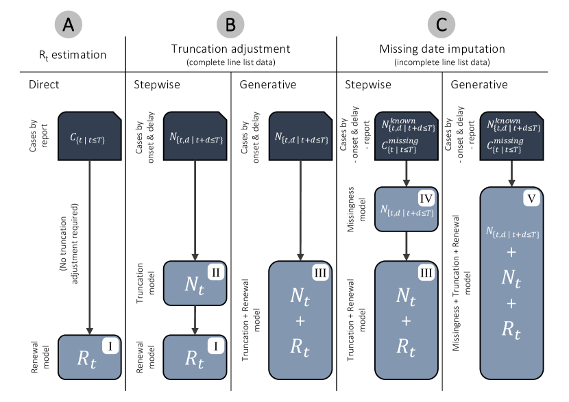
Fig 1: Overview of different approaches for nowcasting the effective reproduction number $R_{t}$. (A) Case counts by date of report are not biased by right truncation and can be used to estimate $R_{t}$ via a direct (no truncation adjustment) approach, assuming knowledge of the delay between infection and report. (B) Case counts by date of symptom onset are only delayed by the incubation period but subject to right truncation. The truncation can be adjusted for by using a stepwise (additional adjustment step) or generative (integrated truncation model) approach. (C) When line list data are incomplete, cases with missing onset date must be accounted for. This can be achieved using a stepwise (additional imputation step) or generative (integrated missingness model) approach. (i@–v@) Models used in the steps of the different approaches. To ensure comparability, the model components for $R_{t}$ estimation, truncation adjustment, and missing date imputation were designed to be maximally similar across all approaches (see SI Appendix B for full model definitions).

2.1 (A) Effective reproduction number estimation

There exist various mechanistic and non-mechanistic approaches to estimate $R_{t}$, most of which rely on the renewal equation[23, 24] as a mathematical foundation. For example, the non-parametric method by Cori et al.[8] implemented in the widely used package EpiEstim allows to compute Bayesian $R_{t}$ estimates efficiently from a time series of case counts. To account for the delay between infection and reporting of cases however, these estimates must be shifted back in time by the mean delay, or one must first infer the time series of infections in an intermediate step using deconvolution[7, 1]. This and other limitations have motivated the recent development of Bayesian methods which model infections and $R_{t}$ as latent variables. Here we use a semi-mechanistic renewal model similar to existing tools[25, 26] to estimate $R_{t}$ directly from observed case counts (Figure 1A). This allows us to specify a single generative model for our data, which can then be adapted to right-truncated and incomplete line lists.

Specifically, we model $C_{t}$, the number of cases by date of report, as Poisson distributed with rate $\lambda_{t}$, the expected number of cases reported on date $t$. We link $\lambda_{t}$ to the number of infections on date $t$, denoted $I_{t}$, via convolution over previous dates, i. e.

$$C_{t}|\lambda_{t}\sim\text{Poisson}(\lambda_{t}),\quad\lambda_{t}=\sum_{d=0}^{D}I_{t-d}\,\rho_{t-d}\,p_{d}$$ (1)

where $\rho_{t-d}$ is an ascertainment proportion, i. e. the proportion of infections at time $t-d$ that eventually become reported cases, and $p_{d}$ the probability of report $d$ days after infection, with an assumed maximum delay $D$. We here let $\rho_{t}=\rho$ for all $t$, i. e. we assume that the ascertainment proportion is constant over time. Importantly, both $\rho$ and $p$ are assumed to be known, and $p$ is typically composed of i) a delay from infection to symptom onset (i. e. the incubation period), and ii) a delay from symptom onset to reporting. The latter is specific to each reporting system and should be estimated from line list data. We here follow the common practice of using the empirical distribution of delays observed in the line list as a proxy for the reporting delay. This naive approach ignores the right truncation of observations and assumes a fixed delay over time, and we assess the bias resulting from this simplification on synthetic data. We remark that a rough estimate of $\rho$ is often sufficient for estimating $R_{t}$, as constant-in-time multipliers cannot bias $R_{t}$ estimates and will distort uncertainty quantification only in extreme cases of misspecification[11]. If $\rho_{t}$ changes over time however, $R_{t}$ estimates will be biased, with slow, constant changes introducing small but continuous bias, and incidental abrupt changes introducing bigger but only temporary bias. In real-world settings, both of these types of changes can occur.

The number of infections $I_{t}$ is modeled via a renewal process as in previous work[2, 27, 28, 29], i. e.

$$I_{t}|\iota_{t}\sim\text{Poisson}(\iota_{t}),\quad\iota_{t}=E[I_{t}]=R_{t}\sum_{s=1}^{G}\psi_{s}\,I_{t-s},$$ (2)

where $\psi$ represents an assumed intrinsic generation time distribution[30] and $G$ is the maximum generation time (see SI Appendix A.2.2 for the modeling of initial infections). Note that we here use a stochastic formulation, i. e. we account for variance in the offspring distribution by sampling realized infections $I_{t}$ as independently Poisson distributed given $\iota_{t}$[31, 27]. As a smoothing prior for $R_{t}$ over time, we use a first-order random walk. To ensure $R_{t}>0$, we apply a softplus link to the random walk, i. e.

$$\text{softplus}^{-1}(R_{t})|R_{t-1}\sim N(\text{softplus}^{-1}(R_{t-1}),{\sigma_{R}}^{2}),$$ (3)

where $\text{softplus}(x)=\frac{\log(1+e^{kx})}{k}$ is the softplus function with sharpness parameter $k$. We choose $k=4$ to ensure that the random walk is effectively on the unit scale for all realistic values of $R_{t}$, thereby modeling changes in $R_{t}$ over time as symmetric (see SI Appendix A.1.3). This reflects our expectation that interventions and behavioral changes have roughly symmetric effects on $R_{t}$[32], but other link functions such as log[25] or generalized logit[26] are also possible. We use weakly informative priors for $R_{1}$ and $\sigma_{R}$ (see SI Appendix A.1.1), to allow the intercept and variance of the random walk to be estimated from the data.

Using Eq. (1)–(3) (full model in SI Appendix B.1), we can compute the likelihood $P\left(C_{\{t|t\leq T\}}\;\middle|\;R_{\{t|t\leq T\}},\theta\right)$ with nuisance parameters $\theta$ and, together with corresponding priors (SI Appendix B.6), sample from the posterior $P\left(R_{\{t|t\leq T\}},\theta\;\middle|\;C_{\{t|t\leq T\}}\right)$ using Markov chain Monte Carlo (MCMC, see Section 2.5) to obtain Bayesian estimates of $R_{t}$ over time.

2.2 (B) Truncation adjustment

The direct estimation of $R_{t}$ from case counts by date of report $C_{t}$ requires a deconvolution of $C_{t}$ with potentially long and difficult-to-estimate delays between infection and reporting. An alternative is to estimate $R_{t}$ from case counts by date of symptom onset $N_{t}$ (Figure 1B), such that the delay distribution in Eq. 1 is simply the incubation period, which is shorter and generally independent of the reporting system. On the present date $T$ however, only $N_{t,d}$ with $t+d\leq T$ are known, such that the real-time count $\sum_{d=0}^{T-t}N_{t,d}$ is a downward-biased estimate of $N_{t}$. This bias must be corrected by estimating the number of symptom onsets which have occurred but are not yet reported, also known in the statistical literature as “nowcasting” in the narrow sense[13]. Conceptually this task is related to time-to-event analysis[33], as it requires estimating the distribution of reporting delays from right truncated observations $N_{t,d}$ to predict the not-yet-reported cases.

Stepwise approach

To nowcast $R_{t}$, existing methods follow a stepwise approach[17, 18, 19], where first $N_{t}$ is estimated using the observed $N_{t,d}$ in a truncation adjustment step, and then $R_{t}$ is estimated from the time series of $N_{t}$ (instead of $C_{t}$, as in Section 2.1). For the truncation adjustment step, we specify a model similar to Günther et al.[17], which jointly combines Bayesian smoothing of the epidemic curve[34, 15] with a discrete time-to-event model for the reporting delay distribution[14]. The latter allows to estimate reporting delays that change over time (e. g. due to changes in the reporting process or the burden on health authorities) and are subject to seasonality (e. g. due to weekday effects), which is both observed in practice[14]. For this, we define $p_{t,d}$ as the probability that a case with symptom onset on date $t$ is reported with a delay of $d\in[0,1,\ldots D]$ days after symptom onset, i. e. we assume that reporting cannot occur before symptom onset (no negative delays) and is at most $D$ days after symptom onset. In practice, it is important to assume a long enough maximum delay $D$ that sufficiently covers the true delay distribution. Cases with delays longer than $D$ should then be completely dropped from the analysis, as setting their delays to $D$ instead can lead to right truncation bias. Given the above definition, we assume that cases with symptom onset on date $t$ are Poisson distributed with rate $\lambda_{t}$, and their reporting delays are categorically distributed with event probabilities $p_{t,d}$. We can then model the observed numbers of cases with symptom onset on date $t$ and reporting delay $d$ as

$$N_{t,d}|\lambda_{t},p_{t,d}\sim\text{Poisson}(\lambda_{t}\,p_{t,d}),$$ (4)

To model the delay probabilities $p_{t,d}$, we use a discrete time-to-event model in which we parameterize the hazard of reporting $h_{t,d}$ via a logistic regression[14, 35], i. e.

$$p_{t,d}=h_{t,d}\,\prod_{i=1}^{d}(1-h_{t,d-i}),\quad\text{logit}(h_{t,d})=\gamma_{d}+z_{t}^{\top}\beta+w_{t+d}^{\top}\,\eta,$$ (5)

where $\gamma_{d}$ is the logit baseline hazard for delay $d$, and $z_{t}$ and $w_{t+d}$ are vectors of covariates with coefficient vectors $\beta$ and $\eta$, respectively. This implements a non-parametric, proportional hazards model[36] for the reporting delay as in Günther et al., however, we here model both effects by date of symptom onset $z_{t}^{\top}\beta$ and effects by date of report $w_{t+d}^{\top}\,\eta$. We design $z_{t}$ to account for changes in the reporting delay of cases over time via a piecewise linear weekly change point model, and $w_{t+d}$ to account for differences in reporting between weekdays (see SI Appendix A.3.1 for details). As a smoothing prior for $\lambda_{t}$ over time, we use a first-order random walk on the log scale, i. e.

$$\log(\lambda_{t})|\lambda_{t-1}\sim N(\log(\lambda_{t-1}),{\sigma_{\log(\lambda)}}^{2}).$$ (6)

This is a minimally informed prior assuming a stationary time series of symptom onsets which has often been used in earlier work[34, 15, 17, 37], and we test non-stationary exponential smoothing as an alternative prior in a supplementary analysis (SI Appendix A.1.2). Analogous to Section 2.1, we use weakly informative priors for $\log(\lambda_{1})$ and $\sigma_{\log(\lambda)}$ (see SI Appendix A.1.1), to estimate the random walk intercept and variance from the data.

Given Eq. (4)–(6) (full model in SI Appendix B.2), we can compute the likelihood $P\left(N_{\{t,d|t+d\leq T\}}\;\middle|\;\lambda_{\{t|t\leq T\}},p_{\{t,d|t\leq T,d\leq D\}},\theta\right)$, and obtain posterior samples $\hat{\lambda}_{\{t|t\leq T\}}^{(i)},\,\hat{p}_{\{t,d|t\leq T,d\leq D\}}^{(i)}\sim P\left(\lambda_{\{t|t\leq T\}},p_{\{t,d|t\leq T,d\leq D\}},\theta\;\middle|\;N_{\{t,d|t+d\leq T\}}\right)$ via MCMC. These can then be used to produce samples of the not-yet-observed case counts $\hat{N}_{\{t,d|t+d>T\}}^{(i)}$ by drawing from $\text{Poisson}(\hat{\lambda}_{t}^{(i)}\hat{p}_{t,d}^{(i)})$, respectively. Samples from the nowcast for $N_{t}$ are then simply obtained by summing up the already observed and the sampled, not-yet-observed case counts, i. e. $\hat{N}_{t}^{(i)}=\sum_{d=0}^{\min(T-t,D)}N_{t,d}+\sum_{d=T-t+1}^{D}\hat{N}_{t,d}^{(i)}$.

To obtain a nowcast for $R_{t}$, existing nowcasting approaches typically estimate $R_{t}$ from the nowcast for $N_{t}$ in a separate step. Since the nowcast for $N_{t}$ is subject to considerable uncertainty on dates close to the present, stepwise approaches must repeat the $R_{t}$ estimation step on many samples $\hat{N}_{\{t|t\leq T\}}^{(i)}$ from the truncation adjustment, and finally combine the resulting $R_{t}$ estimates. This “resampling” procedure is necessary to account for the uncertainty from the truncation adjustment but introduces computational overhead especially if the individual $R_{t}$ estimation steps are costly. In practice, stepwise approaches therefore either ignore uncertainty from the truncation adjustment[38] or use simple, non-parametric methods such as EpiEstim to estimate $R_{t}$[17, 18]. To ensure a consistent comparison of approaches in this study, we fitted the generative model introduced in Section 2.1 on 50 different samples $\hat{N}_{\{t|t\leq T\}}^{(i)}$ using MCMC, which incurred comparatively high computational cost. We additionally produced nowcasts using EpiEstim for $R_{t}$ estimation in a supplementary analysis (SI Appendix A.2.4 and C.1).

Generative approach

As an alternative to the stepwise approach, we here propose to integrate $R_{t}$ estimation and truncation adjustment in a single generative model. This is achieved by replacing Eq. 6 in the truncation adjustment model with

$$\lambda_{t}=\sum_{s=0}^{L}I_{t-s}\,\rho_{t-s}\,\tau_{s},$$ (7)

where $\rho_{t-s}$ is again an assumed ascertainment proportion, $\tau$ is the incubation period distribution, $L$ is the maximum incubation period, and $I_{t}$ is the number of infections on date $t$. Analogous to Section 2.1, infections $I_{t}$ are then modeled via a renewal model using Eq. 2 and Eq. 3. By doing so, we replace the non-parametric smoothing prior for $\lambda_{t}$ with a model of symptom onsets that arise from latent infections generated through a renewal process. This yields a single hierarchical model based on Eq. (2) – (5), and (7) (full model in SI Appendix B.3), under which we can directly compute the joint likelihood

$$P\left(N_{\{t,d|t+d\leq T\}}\;\middle|\;\lambda_{\{t|t\leq T\}},p_{\{t,d|t\leq T,d\leq D\}},R_{\{t|t\leq T\}},\theta\right),$$

and obtain posterior samples for $R_{t}$ and $N_{t}$ as described before. The resulting generative approach allows to nowcast $R_{t}$ and $N_{t}$ in a single step, while quantifying uncertainty both from truncation adjustment and $R_{t}$ estimation. Moreover, by explicitly linking the time series of symptom onsets to the underlying infection dynamics, we use the renewal model as a structural prior for the temporal correlation of $N_{t}$. This way, epidemic modeling is not only used to estimate $R_{t}$ but also to regularize the nowcast for $N_{t}$, thereby avoiding the additional non-parametric smoothing of $\lambda_{t}$ in the stepwise approach.

2.3 (C) Missing date imputation

In practice, line list data are often incomplete, i. e. the date of symptom onset can be missing for a substantial proportion of cases. Ignoring incomplete cases and computing nowcasts as described in Section 2.2 only using the complete cases $N_{t,d}^{\text{known}}$ will underestimate $N_{t}$ and bias nowcasts of $R_{t}$ if the proportion of cases with missing onset date changes over time. It is therefore important to also include the incomplete cases, which are only available as case counts $C_{t}^{\text{missing}}$ by date of report. Here we discuss two stepwise approaches of imputing missing onset dates and then show how a missingness model can be directly integrated into the generative nowcasting model (Figure 1C).

Stepwise approach

A simple but potentially biased approach is to treat the reporting delays of cases in the line list as independent and identically distributed. Under this assumption, missing onset dates can be imputed by simply subtracting a random delay from the date of report of each incomplete case, i. e. each case counted in $C_{t}^{\text{missing}}$. The random delays could for example be drawn from the empirical delay distribution of delays from complete cases in the line list. However, even if there was no right truncation or changes in the reporting delay over time, such a procedure will yield biased results during an epidemic wave. This is because subtracting delays from the date of report implicitly conditions the delay distribution on the date of report[7, 39]. The resulting distribution, also known as backward delay distribution, depends on the shape of the past epidemic curve and therefore varies during an epidemic. A more accurate approach is therefore to only assume that cases with the same date of report have identically distributed delays, and to estimate the so-called backward delay probability $p^{\leftarrow}_{t,d}$ that a case reported on date $t$ had its symptom onset $d$ days ago[17, 18, 19]. We here implement this approach by modeling the number of cases with known symptom onset date as

$$(N_{t,0}^{\text{known}},\dots,N_{t-D,D}^{\text{known}})\sim\text{Multinom}(p^{\leftarrow}_{t,0},\dots,p^{\leftarrow}_{t,D}),$$ (8)

and parameterizing $p^{\leftarrow}_{t,d}$ using an identical discrete time-to-event model as specified in Eq. 5, but indexed by date of report instead of date of symptom onset (SI Appendix B.4). We remark that by conditioning on the date of report, the above model is not biased by right truncation, but potentially by left truncation (see SI Appendix A.3.2). We compute the likelihood $P\left(N_{\{t,d|t+d\leq T\}}^{\text{known}}\;\middle|\;p^{\leftarrow}_{t,d},\theta\right)$ to obtain posterior samples from $P\left(p^{\leftarrow}_{t,d},\theta\;\middle|\;N_{\{t,d|t+d\leq T\}}^{\text{known}}\right)$ via MCMC, and use the latter to impute missing onset dates by drawing random delays from the corresponding backward delay distribution. Importantly, using observed delays to impute missing onset dates implies a missing-at-random assumption, i. e. reporting delays are assumed to be independent of whether cases in the line list are complete or incomplete. Moreover, both the independent imputation and the backward-delay imputation approach are stepwise in that they add an additional imputation step prior to nowcasting. As a result, the imputed symptom onset dates are treated as observed data during the following step(s), which creates the same obstacle to uncertainty quantification as described in Section 2.2. Thus, to account for uncertainty of the imputation, a multiple imputation scheme must be used, where multiple imputed data sets are created and a separate nowcast is estimated for each data set[18]. With more complex nowcasting models however, multiple imputation is often impractical and therefore omitted[17], as fitting to a large number of imputed data sets would be prohibitively computationally expensive. Similarly, we only assessed single imputations due to resource constraints in this study.

Generative approach

As an alternative, we propose to directly account for missing symptom onset dates in the generative nowcasting model described in Section 2.2. For this, we assume that symptom onsets on date $t$ become known with probability $\alpha_{t}$ and missing with probability $1-\alpha_{t}$. The case counts with known and missing symptom onset date $t$ and delay $d$ are then modeled as

$$N_{t,d}^{\text{known}}|\lambda_{t},p_{t,d},\alpha_{t}\sim\text{Poisson}(\lambda_{t}\,p_{t,d}\,\alpha_{t}),\quad N_{t,d}^{\text{missing}}|\lambda_{t},p_{t,d},\alpha_{t}\sim\text{Poisson}(\lambda_{t}\,p_{t,d}\,(1-\alpha_{t})),$$ (9)

which again assumes that symptom onset dates are missing at random, i. e. independent of their reporting delay. While the $N_{t,d}^{\text{missing}}$ are not directly observed in the line list, we know that $C_{t}^{\text{missing}}=\sum_{d=0}^{\min(D,t-1)}N_{t-d,d}^{\text{missing}}.$ Hence, $C_{t}^{\text{missing}}$ is the sum of Poisson distributed case numbers from previous days with corresponding delays, and it is also Poisson distributed with

$$C_{t}^{\text{missing}}|\lambda,p,\alpha\sim\text{Poisson}\left(\sum_{d=0}^{\min(D,t-1)}\lambda_{t-d}\,p_{t-d,d}\,(1-\alpha_{t-d})\right).$$ (10)

Note that under this model, only observations $C_{t}^{\text{missing}}$ for $t>D$ should be used to avoid bias from left-truncation, or the latent parameters $\lambda$, $p$, and $\alpha$ must be further extended into the past (SI Appendix A.4). As a minimally informed, stationary smoothing prior for $\alpha_{t}$ over time, we use a first-order random walk on the logit scale, i. e.

$$\text{logit}(\alpha_{t})|\alpha_{t-1}\sim N(\text{logit}(\alpha_{t-1}),{\sigma_{\text{logit}(\alpha)}}^{2}),$$ (11)

and estimate $\alpha_{1}$ and $\sigma_{\text{logit}(\alpha)}$ with weakly informed priors as before. This assumes that the probability of missing symptom onset dates varies only by date of symptom onset, but more sophisticated models could also account for weekday effects or effects by date of report. Assuming $N_{t,d}^{\text{known}}$ and $C_{t}^{\text{missing}}$ as independent given $\lambda$, $p$, and $\alpha$, we can replace Eq. 4 in the existing hierarchical nowcasting model described in Section 2.2 with Eq. (9), (10), and (11) (full model in SI Appendix B.5). Under the resulting model, we can compute the joint likelihood

$$P\left(N_{\{t,d|t+d\leq T\}}^{\text{known}},C_{\{t|t\leq T\}}^{\text{missing}}\;\middle|\;\lambda_{\{t|t\leq T\}},p_{\{t,d|t\leq T,d\leq D\}},\alpha_{\{t|t\leq T\}},R_{\{t|t\leq T\}},\theta\right)$$

and obtain posterior samples for $R_{t}$ and $N_{t}$ using MCMC as before. Therefore, the model can be jointly fit to incomplete line list data without the need for an additional imputation step. This also accounts for the uncertainty resulting from missing onset dates without the use of a multiple imputation scheme. In comparison to stepwise approaches, the generative approach requires estimating the probability of missing onset dates over time, but in turn avoids estimating backward-delay distributions. Moreover, using estimates for $\alpha_{t}$, separate nowcasts for $N_{t}^{\text{known}}$ and $N_{t}^{\text{missing}}$ can be easily obtained.

2.4 Modeling of overdispersion

As found in earlier work[17], the modeling of overdispersed case counts can improve nowcasting performance in real-world settings. When nowcasting COVID-19 hospitalizations in Switzerland, we therefore model observed case counts as Negative Binomial instead of Poisson distributed in all our models, e. g. we use

$$N_{t,d}|\lambda_{t},p_{t,d},\phi\sim\text{NegBin}(\lambda_{t}\,p_{t,d},\phi),$$ (12)

instead of Eq. 4, where the inverse of $\phi$ defines the level of overdispersion, with $Var[N_{t,d}|\lambda_{t},p_{t,d},\phi]=(\lambda_{t}\,p_{t,d})(1+\frac{\lambda_{t}\,p_{t,d}}{\phi})$. We place a prior on $\frac{1}{\sqrt{\phi}}$ to regularize the overdispersion (SI Appendix B.6) and use a pooled overdispersion parameter for all observations.

2.5 Implementation and estimation

We implemented all models used in the different nowcasting approaches (Figure 1) as probabilistic programs in Stan[40] (SI Appendix C.1). This allowed us to estimate all parameters in a fully Bayesian framework with Markov chain Monte Carlo (MCMC) using cmdstan version 2.30.0 via cmdstanr version 0.5.0[41]. To provide regularization, we used weakly informative priors on the model parameters (see SI Appendix B.6 for details). For each estimation, the default configuration of the No-U-Turn sampler was run, i. e. four chains with 1,000 warm-up and 1,000 sampling iterations each. After model fitting, we computed common Bayesian model diagnostics to check for convergence (Gelman-Rubin convergence diagnostic $\hat{R}$)[42] and sufficient sample sizes (ESS ratio)[43] (SI Appendix C.3). We used the R package EpiEstim[8] for $R_{t}$ estimation with the method by Cori et al., and the R package scoringutils[44] for computation of weighted interval scores. All processing steps and analyses were performed in R 4.1.0, and the models and code for this study are available from zenodo at https://doi.org/10.5281/zenodo.8279676.

2.6 Comparison of approaches using synthetic data

We used synthetic data to compare the different stepwise and generative nowcasting approaches. To simulate synthetic data, we generated infections through a stochastic renewal process over a period of 200 days in which $R_{t}$ follows a piecewise linear time series with prespecified change points. The simulation matches the generative models described in Sections 2.1 and 2.2, but simulates the reporting of individual cases and therefore does not assume independent observation noise. We simulated two different scenarios, representing a first and second epidemic wave, respectively (SI Appendix D.1.1). The first wave scenario starts with a small number of seeding infections and strong transmission ($R_{t}=2$), followed by a shift to suppression ($R_{t}=0.8$). The second wave scenario starts with moderate case numbers and controlled transmission ($R_{t}=1$), followed by a resurgence ($R_{t}=1.4$) and finally decline ($R_{t}=0.8$). For each scenario, we produced 50 simulation runs with different realizations of the infection process. We parameterized the generation interval and the incubation period distributions based on estimates for COVID-19 from the literature[45, 46], and supplied the same distributions to the nowcasting models. To mimic the ascertainment of hospitalization data, we let infections become reported hospitalizations with probability $\rho=2\%$. For each simulation run, we obtained a synthetic line list by simulating the symptom onset and day of report of each case. The baseline reporting delay was specified as a discretized gamma distribution with a mean of 9 days and standard deviation of 8 days, which is in line with the delay between symptom onset and reporting of hospitalization during the first year of the COVID-19 pandemic in Switzerland (SI Appendix Figure 15). We used a piecewise linear model to simulate changes in the reporting hazard over time, with random changes in the trend every four weeks, which differed across simulation runs. We also included weekday effects with the odds of reporting being at the baseline Wednesday – Friday, 70% lower on Saturdays, 80% lower on Sundays, 10% higher on Mondays, and 5% higher on Tuesdays. Details of the simulation of infections and reporting are provided in SI Appendix D.

For each simulation run and scenario, nowcasts were obtained for selected weeks in different phases of the epidemic wave (Figure 2–5, SI Appendix B.6) by applying the nowcasting approaches at different lags of the respective week (at the end of the week, one week after, two weeks after). This allowed us to assess changes in performance as more data becomes available. We fitted the models using always the last three months of line list data until the date of the nowcast. Complete line list data, i. e. without missing symptom onset dates, were used to compare the direct $R_{t}$ estimation with the stepwise and generative truncation adjustment approaches. Incomplete line list data were used to compare the stepwise and the generative missing date imputation approaches. Here we randomly selected cases to have a missing symptom onset date with a probability varying over time between 20% and 60% according to a random piecewise linear function, which differed across simulation runs.

To evaluate nowcasting performance in each of the 50 simulation runs, we scored the nowcasts for each week in each phase with respect to $N_{t}$ and $R_{t}$ against the simulated ground truth. As a performance measure, we used the weighted interval score (WIS), which is a quantile-based proper scoring rule that approximates the continuous ranked probability score (CRPS). The CRPS generalizes the absolute error to probabilistic nowcasts. For an observation $y$, i. e. the true $N_{t}$ or $R_{t}$, and a predictive distribution $F$, i. e. the probabilistic nowcast for $N_{t}$ or $R_{t}$, the weighted interval score is computed as

$$\text{WIS}(F,y)=\frac{1}{2K+1}\left(|y-F_{0.5}|+\sum_{k=1}^{K}(\alpha_{k}\,\text{IS}_{\alpha_{k}}(F,y))\right),$$ (13)

where $|y-F_{0.5}|$ is the absolute error of the median, $\alpha_{k}\in\{\alpha_{1},\dots,\alpha_{K}\}$ represent different central prediction intervals at coverage level $(1-\alpha_{k})$, and $\text{IS}_{\alpha}(F,y)$ is the interval score for a specific interval, defined as

$$\text{IS}_{\alpha}(F,y)=\underbrace{\vphantom{\frac{2}{\alpha}}(F_{1-\frac{\alpha}{2}}-F_{\frac{\alpha}{2}})}_{\text{dispersion}}+\underbrace{\frac{2}{\alpha}(y-F_{1-\frac{\alpha}{2}})\mathds{1}_{y>F_{1-\frac{\alpha}{2}}}}_{\text{underprediction}}+\underbrace{\frac{2}{\alpha}(F_{\frac{\alpha}{2}}-y)\mathds{1}_{y<F_{\frac{\alpha}{2}}}}_{\text{overprediction}}.$$ (14)

That is, the interval score can be decomposed into three penalty components, where the dispersion component encourages sharpness, and the under- and overprediction components encourage calibration of the nowcast. We used $K=11$ different $\alpha_{k}$, corresponding to the 10%, 20%, $\dots$, 90%, 95%, and 98% credible intervals (CrI) for $N_{t}$ and $R_{t}$, respectively. To obtain an overall score $\overline{\text{WIS}}$ for each evaluated week, we took the arithmetic mean of scores from each day of the week, which again yields a proper score. We furthermore computed the relative contribution of each penalty component (dispersion, over-, and underprediction) to the respective $\overline{\text{WIS}}$. In the results, we report the average $\overline{\text{WIS}}$ over all 50 simulation runs, as well as the percentage of runs where each approach performed best.

2.7 Application to COVID-19 in Switzerland

We also compared the direct, stepwise, and generative nowcasting approaches during the COVID-19 pandemic in Switzerland. For this, we used anonymized line list data of cases reported to the Federal Office of Public Health (FOPH) from January 01, 2020 – March 31, 2021. Because in Switzerland the date of symptom onset for COVID-19 was only consistently recorded for hospitalized patients, we only used cases of hospitalization from the line list. As date of report, the date when a hospitalization was recorded by FOPH was used. The symptom onset date was either reported together with the clinical record of hospitalization or slightly before (due to a previous test result which was later merged), but not updated afterward. Negative delays were therefore assumed to be data entry errors, and the respective symptom onset dates were set to missing.

We produced retrospective nowcasts for the number of hospitalizations by date of symptom onset $N_{t}$ (including cases with and without known symptom onset) and the effective reproduction number $R_{t}$ during different phases of the first and second wave (before, at, and after peak, respectively). We assumed a maximum delay of 8 weeks, which covered 97.03% of reporting delays, and removed the small percentage of cases with larger delays from the analysis. When modeling weekday effects on the reporting delay, we coded national public holidays in Switzerland as Sundays. To account for the gradual replacement of the SARS-CoV-2 wild-type by the alpha variant from December 2020 – April 2021, we used different incubation period distributions ($\tau^{\text{wild-type}}=\Gamma(\alpha=2.74,\beta=0.52)$[45], $\tau^{\text{alpha}}=\Gamma(\alpha=3.08,\beta=0.63)$[47]) and generation interval distributions ($\psi^{\text{wild-type}}=\Gamma(\alpha=1.43,\beta=0.29)$[46], $\psi^{\text{alpha}}=\Gamma(\alpha=1.75,\beta=0.38)$[48]) over time according to a logistic growth transition (SI Appendix E.2).

On real-world data, the nowcasting performance with regard to $N_{t}$ can be evaluated in retrospect by observing the number of cases with a certain onset date after a sufficiently long delay. This is however only possible for cases with known onset date, i. e. $N_{t}^{\text{known}}$. To obtain a proxy ground truth for $N_{t}^{\text{missing}}$, we used nowcasts at large lags beyond the respective date (7–14 days more than the maximum delay). These nowcasts are informed by fully reported case counts and thus no longer subject to right truncation. The resulting “consolidated” estimates of the true $N_{t}$ were used to evaluate the performance of the different real-time nowcasts with regard to $N_{t}$, using the same weighted interval scoring rule as described for the synthetic data. Since the effective reproduction number $R_{t}$ cannot be observed in a real-world setting, and corresponding estimates are subject to considerable uncertainty, we refrained from assessing the performance of $R_{t}$ nowcasts and focused on a qualitative comparison instead.

3 Results

3.1 Synthetic data: $R_{t}$ estimation and truncation adjustment

We used complete synthetic line list data, i. e. without missing symptom onset dates, to compare i) the direct $R_{t}$ estimation approach, ii) the stepwise nowcasting approach with an additional truncation adjustment step, and iii) the generative nowcasting approach with a joint truncation and renewal model.

3.1.1 Nowcasts of the number of cases by symptom onset date $N_{t}$

Figure 2 shows the simulated true $N_{t}$ and corresponding nowcasts for an exemplary simulation run in different phases of the first wave scenario (corresponding results for the second wave scenario are shown in SI Appendix Fig. 4). The baseline simulated reporting delay had a mean of 9 days and standard deviation of 8 days, and the maximum assumed delay was $D=56$ days. The nowcasts were conducted using the different approaches and at different lags (nowcast at end of same week, one week after, two weeks after). The direct $R_{t}$ estimation approach did not produce nowcasts for $N_{t}$, as it directly uses counts by date of report $C_{t}$ instead.

Compared to $C_{t}$, which includes reporting delays, the time series of $N_{t}$ tracked transmission dynamics in a more timely and regular manner (SI Appendix Fig. 2-3). In a real-time setting however, the reported number of symptom onsets can have a substantial downward bias towards the present (Figure 2, grey bars), because a proportion of symptom onsets that occur close to the present are not yet reported at the time of nowcasting. This truncation bias was adjusted for both by the stepwise and generative approach, however, nowcasts differed between the two approaches especially on dates close to the present.

While the generative approach predicted exponentially growing or declining case counts before and after the peak of the wave, the stepwise approach predicted case counts to remain at the recent level in all phases. This qualitative difference was strongest for nowcasts conducted at short lags, where nowcasting uncertainty was especially high, and declined with longer lags, as more data became available for the respective week.

Below each lag and phase, Figure 2 and SI Appendix Fig. 4 show the weighted interval score (WIS) for each approach across 50 simulation runs. The generative approach achieved systematically better scores in phases with exponential growth or decline, while the stepwise approach had a bias towards underprediction of $N_{t}$ during exponential growth and towards overprediction during decline. This further highlights the difference in smoothing assumptions of the two approaches. While the renewal model component in the generative approach predicted a continuation of recent infection dynamics, the minimally informed random walk prior in the stepwise approach predicted stationary case counts. Notably, at the peak of the wave, this led the generative approach to overpredict case counts, however only at short lags (same week nowcast), when little signal on the change in transmission dynamics was available. Overall, the WIS for both approaches decreased substantially with larger lags, and nowcasts conducted two weeks after the evaluation period show little difference in performance between the stepwise and the generative approach.

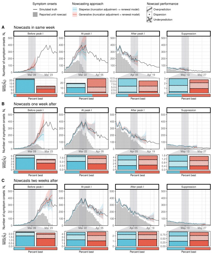
Fig 2: Nowcasts of $N_{t}$ on line list data of a simulated first wave scenario using different approaches of adjusting for right truncation. Shown are the true number of cases by symptom onset date $N_{t}$ (black), the number of cases reported until the nowcast date (grey bars), and point nowcasts with 95% credible intervals (CrI) in four different phases of the epidemic wave, obtained through i) a stepwise approach using cases by date of symptom onset with a truncation adjustment step (blue), and ii) a generative approach using cases by date of symptom onset with an integrated truncation and renewal model (red). The direct approach using cases by date of report does not produce nowcasts of $N_{t}$ (not shown). Shown below each phase is the weighted interval score (WIS, lower is better) for $N_{t}$ nowcasts of each approach during a selected week (grey shade) over 50 scenario runs. Colored vertical bars show average scores, decomposed into penalties for underprediction (crosshatch), dispersion (circles), and overprediction (stripes). The horizontal proportion bar below shows the percentages of runs where each approach performed best. Results are shown for nowcasts made at different lags from the selected week (vertical dotted lines), i. e. at the end of the selected week (top row), one week later (middle row), and two weeks later (bottom row).

3.1.2 Nowcasts of the effective reproduction number $R_{t}$

Figure 3 shows results for nowcasting $R_{t}$ in different phases of the first wave scenario (corresponding results for the second wave scenario are shown in SI Appendix Fig. 5). Here we found distinct biases in the direct and the stepwise approach. The direct $R_{t}$ estimation approach, which used the empirical distribution of delays between symptom onset and reporting in the line list to model observed cases $C_{t}$, showed a strong downward bias of $R_{t}$ nowcasts during the first wave, where few cases had been observed initially. This reflects the right truncation of line list data, which generally leads to an underestimation of reporting delays and therefore of infections in the recent past. In the second wave scenario, the effect of right truncation was smaller. However, due to the long delay between infection and reporting in case counts $C_{t}$, changes in $R_{t}$ were detected comparatively late by the direct $R_{t}$ estimation approach. The stepwise truncation adjustment approach showed a different form of bias, i. e. nowcasts tended to $R_{t}=1$ towards the present, which translated into under- or overprediction of $R_{t}$ depending on the epidemic phase. Importantly, this was observed although the $R_{t}$ estimation step of the stepwise approach used a smoothing prior which expects $R_{t}$ to remain at its current level. This indicates that the $R_{t}$ estimation step was also impacted by the stationary smoothing assumption in the previous truncation adjustment step, i. e. the constant $N_{t}$ nowcasts biased the downstream $R_{t}$ estimates towards equilibrium-level transmission. The generative approach did not show such a bias and generally achieved the smallest WIS among the three approaches. Where no sufficient signal for a change in transmission dynamics was available, $R_{t}$ nowcasts from the generative approach remained at the current level. At the peak of the epidemic wave, when transmission declined from $R_{t}=2$ to $R_{t}=0.8$, this led to an overprediction of $R_{t}$ for nowcasts in the same week. For all approaches, performance scores improved with larger lags, however, the inferior performance of the direct approach in the first wave scenario was pronounced even for nowcasts at a two-week lag.

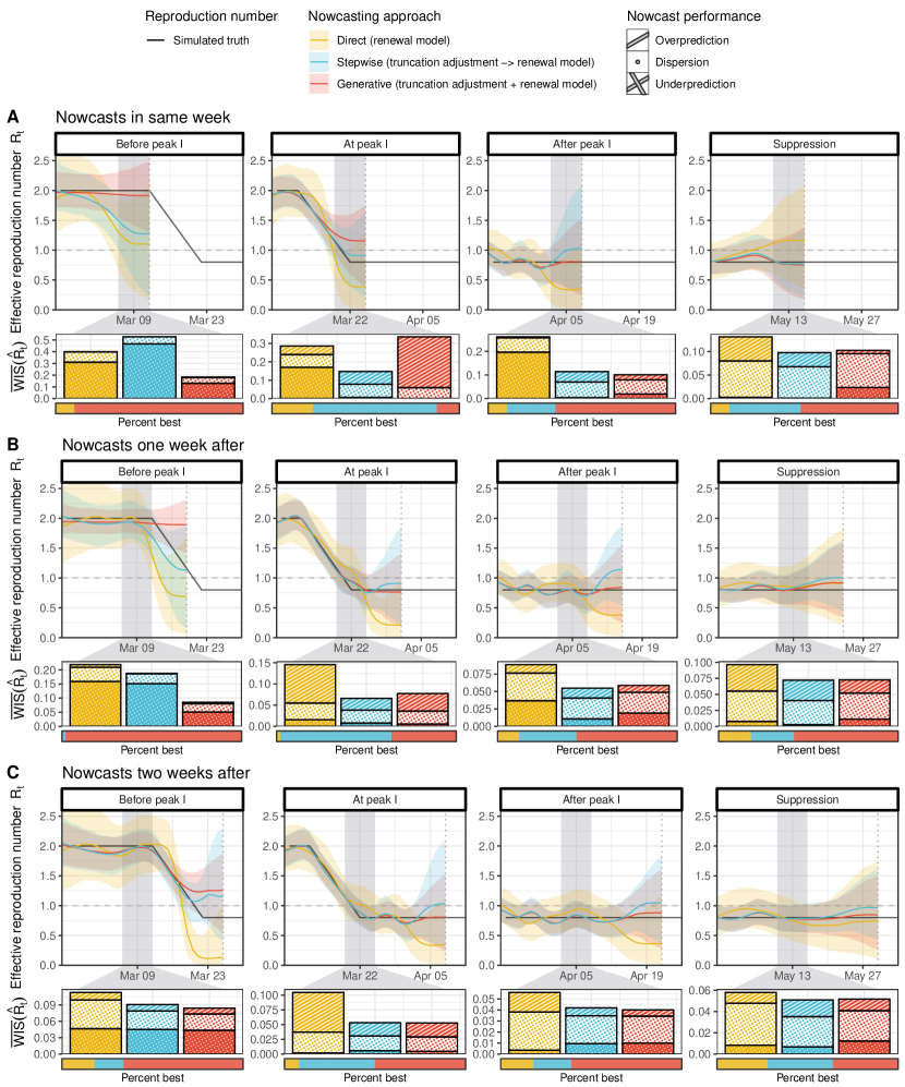
Fig 3: Nowcasts of $R_{t}$ on line list data of a simulated first wave scenario using different approaches of adjusting for right truncation. Shown are the true $R_{t}$ (black) and point nowcasts with 95% credible intervals (CrI) in four different phases of the epidemic wave, obtained through i) a direct approach using cases by date of report with no truncation adjustment (yellow), ii) a stepwise approach using cases by date of symptom onset with a truncation adjustment step (blue), and iii) a generative approach using cases by date of symptom onset with an integrated truncation and renewal model (red). Shown below each phase is the weighted interval score (WIS, lower is better) for $R_{t}$ nowcasts of each approach during a selected week (grey shade) over 50 scenario runs. Colored bars show average scores, decomposed into penalties for underprediction (crosshatch), dispersion (circles), and overprediction (stripes). The horizontal proportion bar below shows the percentages of runs where each approach performed best. Results are shown for nowcasts made at different lags from the selected week (vertical dotted lines), i. e. at the end of the selected week (top row), one week later (middle row), and two weeks later (bottom row).

3.1.3 Additional comparisons

In the above comparisons, a random walk prior on the expected number of symptom onsets was used in the truncation adjustment step of the stepwise approach. While this smoothing prior has been a default choice in existing approaches[34, 15, 17, 37], we also implemented a non-stationary, exponential smoothing prior (SI Appendix A.1.2) to test whether the observed bias in nowcasts remained. We found that non-stationary smoothing in the stepwise approach reduced the bias of both $N_{t}$ and $R_{t}$ nowcasts and improved the WIS, but a slight bias remained during phases of exponential growth or decline (SI Appendix Fig. 8–11). We also tested the use of a non-stationary smoothing prior on $R_{t}$ for the generative approach, which led to slightly better performance of $R_{t}$ nowcasts when transmission was changing.

As it is widely used in practice, we also implemented a stepwise approach where the $R_{t}$ estimation step is performed using the non-parametric method by Cori et al. via the package EpiEstim (SI Appendix A.2.4), instead of our semi-mechanistic renewal model described in Section 2.1. Since the $R_{t}$ estimation step does not influence the previous truncation adjustment step, nowcasts for $N_{t}$ with EpiEstim were identical compared to when using a semi-mechanistic renewal model. The nowcasts for $R_{t}$ showed the same bias towards $R_{t}=1$, however, they were often more volatile and at the same time considerably less uncertain (SI Appendix Fig. 12–13) when using EpiEstim in the $R_{t}$ estimation step. This overconfidence generally led to higher WIS values of the stepwise approach with EpiEstim. We note that when using EpiEstim, nowcasts for $R_{t}$ could only be obtained at a lag of 8 days or more, as $R_{t}$ estimates must be shifted backward in time to account for the incubation period and to center the 7-day smoothing window used for EpiEstim[7].

3.2 Synthetic data: Missing symptom onset date imputation

To compare the different stepwise and generative approaches to impute missing onset dates, we used the same synthetic line list data as before, but simulated symptom onset dates to be missing with a time-varying probability $1-\alpha_{t}$ (Section 2.6). We tested i) a stepwise approach using independent imputation for the imputation step, ii) a stepwise approach using backward(-delay) imputation for the imputation step, and iii) a generative approach using an integrated missingness model. All three approaches used a generative model for truncation adjustment and $R_{t}$ estimation as defined in Section 2.2, allowing us to specifically assess differences resulting from the imputation approach.

Figure 4 shows the simulated true $N_{t}$ and nowcasts for an exemplary simulation run and performance scores over 50 runs in different phases of the first wave scenario (second wave scenario shown in SI Appendix Fig. 6). A strong downward bias in the number of symptom onsets reported until the date of the nowcast was observed both for cases with known and with missing onset date (Figure 4, grey and light grey bars). $N_{t}$ nowcasts conducted at the end of the same week were highly similar for all three approaches, however, differences were observed for longer lags, i. e. one and two weeks after. Here, nowcasts from the generative approach consistently achieved a better WIS than the stepwise approaches. Nowcasts from the stepwise approach with independent imputation, which ignores the conditioning on the date of report, tended to underpredict the peak of the wave, and this bias increased with longer lags, as more data became available. In contrast, the stepwise approach with backward-delay imputation was generally unbiased, with approximately equal penalties for over- and under-prediction. However, as uncertainty from the imputation step was ignored, this approach yielded overconfident nowcasts at larger lags. Nowcasts from the generative approach generally had the widest uncertainty intervals.

Figure 5 and SI Appendix Fig. 7 show the corresponding results for nowcasts of $R_{t}$ in the first and second wave scenario, respectively. The three approaches to missing date imputation produced mostly similar $R_{t}$ nowcasts both at shorter and longer lags, but we observed a small bias of the stepwise approach with independent imputation around the change point of $R_{t}$ due to the underprediction of the peak in $N_{t}$. However, the differences in performance between the approaches were not consistent across phases and comparatively small with regard to the overall WIS, which was dominated by the uncertainty and error from the truncation adjustment and $R_{t}$ estimation.

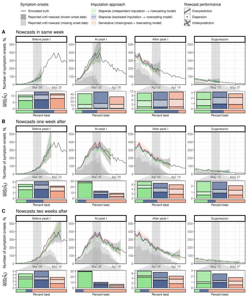
Fig 4: Nowcasts of $N_{t}$ on incomplete line list data of a simulated first wave scenario using different approaches to account for missing onset dates. Shown are the true number of cases by symptom onset date $N_{t}$ (black), the number of cases reported until the nowcast date (dark grey bars for known, light grey bars for missing onset dates), and point nowcasts with 95% credible intervals (CrI) in four different phases of the epidemic wave, obtained through i) a stepwise approach using a forward imputation step (green), ii) a stepwise approach using a backward imputation step (blue), and iii) a generative approach using an integrated missingness model (red). All approaches used a generative model for nowcasting. Shown below each phase is the weighted interval score (WIS, lower is better) for $N_{t}$ nowcasts of each approach during a selected week (grey shade) over 50 scenario runs. Colored bars show average scores, decomposed into penalties for underprediction (crosshatch), dispersion (circles), and overprediction (stripes). The horizontal proportion bar below shows the percentages of runs where each approach performed best. Results are shown for nowcasts made at different lags from the selected week (vertical dotted lines), i. e. at the end of the selected week (top row), one week later (middle row), and two weeks later (bottom row).

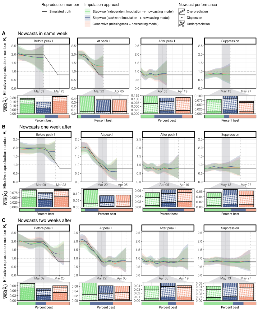
Fig 5: Nowcasts of $R_{t}$ on incomplete line list data of a simulated first wave scenario using different approaches of accounting for missing onset dates. Shown are the true $R_{t}$ (black) and point nowcasts with 95% credible intervals (CrI) in four different phases of the epidemic wave, obtained through i) a stepwise approach using a forward imputation step (green), ii) a stepwise approach using a backward imputation step (blue), and iii) a generative approach using an integrated missingness model (red). All approaches used a generative model for nowcasting. Shown below each phase is the weighted interval score (WIS, lower is better) for $R_{t}$ nowcasts of each approach during a selected week (grey shade) over 50 scenario runs. Colored bars show average scores, decomposed into penalties for underprediction (crosshatch), dispersion (circles), and overprediction (stripes). The horizontal proportion bar below shows the percentages of runs where each approach performed best. Results are shown for nowcasts made at different lags from the selected week (vertical dotted lines), i. e. at the end of the selected week (top row), one week later (middle row), and two weeks later (bottom row).

3.3 COVID-19 hospitalizations in Switzerland

We used line list data of hospitalized patients who tested positive for SARS-CoV-2 during the COVID-19 pandemic in Switzerland, reported between January 01, 2020 – March 31, 2021, to retrospectively nowcast the number of hospitalizations by date of symptom onset and the effective reproduction number. Overall, the line list contained 25,831 cases of hospitalization, with symptom onset missing for 33% of the cases (SI Appendix Fig. 14). 137 cases had a symptom onset date later than the date of report, in which case the symptom onset date was likely a data entry error and set to missing (see Section 2.7). Our assumed maximum delay of $D=56$ days covered 97% of observed reporting delays (SI Appendix Fig. 15), and cases with larger delays were removed from the analysis. We assumed different incubation period and generation time distributions for the wildtype and alpha variants of SARS-CoV-2 and accounted for the introduction and spread of the alpha variant during the second wave in Switzerland (see Section 2.7). Nowcasts were conducted using i) the direct $R_{t}$ estimation approach, ii) a fully stepwise approach (using a backward-delay imputation step, a truncation adjustment step, and an $R_{t}$ estimation step), and iii) a fully generative approach (using a joint missingness, truncation, and renewal model).

Figure 6 shows nowcasts of $N_{t}$, i. e. the number of hospitalizations by date of symptom onset, in different phases of the first and second COVID-19 wave in Switzerland. In contrast to nowcasts by date of hospitalization, these estimates include cases that have developed symptoms but are not yet hospitalized, and thus present a more timely indicator of the underlying infection dynamics. Here we found the same qualitative differences between the generative and the stepwise approach as on synthetic data. In particular, nowcasts from the stepwise approach remained mostly stationary on days close to the nowcast date, while nowcasts from the generative approach extrapolated the recent trend of exponential growth or decline. To assess real-time nowcasting performance with regard to $N_{t}$, we used consolidated estimates based on nowcasts lagged by 7–14 days beyond the maximum delay as a proxy ground truth (see Section 2.7). Based on the consolidated estimates, the generative approach achieved a better WIS in all phases except at the peak of the wave. Nowcasts from the stepwise approach were slightly sharper than from the generative approach at larger lags, likely because of the neglected uncertainty from the missing onset date imputation. Of note, both nowcasting approaches underpredicted $N_{t}$ in the early phase of the epidemic in Switzerland, presumably due to an underestimation of the reporting delay based on very few initial hospitalization cases. Figure 7 shows corresponding nowcasts for the hospitalization-based $R_{t}$. Generally, we found $R_{t}$ nowcasts at a lag below one week to be largely dominated by the smoothing prior of the nowcasting model. This is partly to be expected, as transmission dynamics are additionally delayed by the incubation period, which was on average $\approx 5$ days in our case, thus real-time estimates for $R_{t}$ are generally less informed than for $N_{t}$. Of note, nowcasts using the direct $R_{t}$ estimation approach, which is based on the more delayed case counts $C_{t}$, were dominated by the smoothing prior even longer, until a lag of two weeks or more. $R_{t}$ nowcasts from the fully stepwise and fully generative approach mostly agreed after a lag of two weeks but showed systematic differences at shorter lags. Specifically, as in our results on synthetic data, nowcasts from the stepwise approach tended toward $R_{t}=1$, while nowcasts from the generative approach predicted $R_{t}$ to remain at its current level. Nowcasting uncertainty was mostly similar between the stepwise and the generative approach.

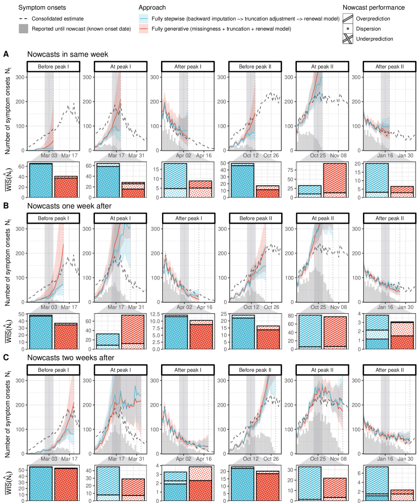
Fig 6: Nowcasts of $N_{t}$ on incomplete hospitalization line list data during the COVID-19 pandemic in Switzerland. Shown are nowcasts with 95% credible interval (CrI) for the number of hospitalizations with COVID-19 by date of symptom onset $N_{t}$ in different phases of the first and second wave, obtained through i) a fully stepwise approach using cases by date of symptom onset with a backward imputation step and a truncation adjustment step (blue), and ii) a fully generative approach using an integrated missingness, truncation and renewal model (red). The direct approach using cases by date of report does not produce nowcasts of $N_{t}$ (not shown). Also shown are the number of cases by symptom onset date reported until the respective nowcast date (grey bars), and consolidated point estimates (7–14 days after maximum delay, averaged over all models) of the true $N_{t}$ (black dashed lines). Shown below each phase is the weighted interval score (WIS, lower is better) for $N_{t}$ nowcasts of each approach during a selected week (grey shade) evaluated on the consolidated point estimates. The scores (colored bars) are decomposed into penalties for underprediction (crosshatch), dispersion (circles), and overprediction (stripes). Results are shown for nowcasts made at different lags from the selected week (vertical dotted lines), i. e. at the end of the selected week (top row), one week later (middle row), and two weeks later (bottom row).

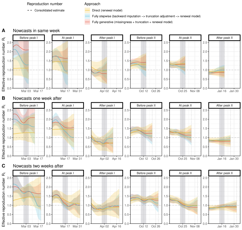
Fig 7: Nowcasts of $R_{t}$ on incomplete hospitalization line list data during the COVID-19 pandemic in Switzerland. Shown are nowcasts with 95% credible interval (CrI) for the effective reproduction number $R_{t}$ in different phases of the first and second wave, obtained from hospitalization line list data through i) a direct approach using cases by date of report with no truncation adjustment (yellow), ii) a fully stepwise approach using cases by date of symptom onset with a backward imputation step and a truncation adjustment step (blue), and iii) a fully generative approach using cases by date of symptom onset with an integrated missingness, truncation, and renewal model (red). Results are shown for nowcasts made at different lags from the selected week (vertical dotted lines), i. e. at the end of the selected week (top row), one week later (middle row), and two weeks later (bottom row).

4 Discussion

In this paper, we developed a fully generative model to nowcast the effective reproduction number $R_{t}$ from right-truncated line list data with missing symptom onset dates. Previous methods have addressed this task by separating missing onset date imputation, truncation adjustment, and $R_{t}$ estimation into consecutive, independent steps[17, 18, 19]. Here we proposed to unify these tasks in a single generative model that can be fit directly to observed data. With such a model, all quantities of interest and their associated uncertainty can be estimated jointly in a Bayesian framework. This is in contrast to stepwise approaches, which face difficulties in propagating uncertainty between consecutive steps and often require resampling schemes that can restrict the individual components. Moreover, information can only flow in one direction, such that priors and model structure from later steps cannot inform earlier steps. Instead, our generative model enables shared regularization between imputation, truncation adjustment, and $R_{t}$ estimation, thereby eliminating the need for non-parametric smoothing at intermediate steps.

To compare the generative and the stepwise approaches with regard to performance and qualitative behavior, we applied them to synthetic line list data for different outbreak scenarios and to real-world data of hospitalizations during the COVID-19 pandemic in Switzerland. We found that under realistic delays between symptom onset and reporting of hospitalized cases, nowcasts for days close to the present are based on few reported cases and thus can be substantially influenced by prior assumptions about the smoothness and shape of the epidemic curve. In nowcasting practice, it is therefore important to be aware that under long reporting delays, real-time nowcasts can effectively become weakly informed forecasts due to a lack of data signal.

When nowcasting $R_{t}$, estimates can be obtained either from case counts by date of report $C_{t}$, or from case counts by date of symptom onset $N_{t}$. The approach using $C_{t}$ can be more direct as it requires no truncation adjustment of case counts, but it depends on external estimates of the reporting delay distribution to infer the time series of infections. Our results show that the resulting $R_{t}$ estimates can still be substantially biased when using naive empirical estimates of the reporting delay. On the other hand, approaches using cases by date of symptom onset are more complex as they must adjust for the right truncation of the real-time case count. Existing methods conduct this truncation adjustment in a separate step, and we found that this can systematically over- and underpredict case counts depending on the current epidemic phase. Specifically, we demonstrated that when modeling the expected number of cases via a stationary random walk - as customary in earlier studies[17, 34, 18, 15, 37] - nowcasts will be biased during periods of exponential growth or decline. Notably, our results show that the stationary smoothing can even overwrite prior assumptions in the subsequent $R_{t}$ estimation step and therefore bias the $R_{t}$ estimates towards $R_{t}=1$. In our proposed generative approach, the renewal model assumed for $R_{t}$ estimation also serves as an epidemiologically motivated smoothing prior for the case counts. As a result, the generative model achieved better nowcasts of $N_{t}$ and $R_{t}$ in phases of epidemic growth or decline by extrapolating the current growth dynamics. At the immediate peak of the epidemic curve, this led to a higher chance of overpredicting $N_{t}$, which is a generally known trade-off in renewal modeling but at the same time the preferred minimal assumption absent a sufficient signal of changes in transmission[49]. Overall, our findings highlight the importance of adequate smoothing priors for nowcasting under long delays, and demonstrate how model misspecification can impact downstream estimates in stepwise modeling pipelines.

When nowcasting from incomplete line list data with missing symptom onset dates, we found that even with up to 60% of missing data, informative nowcasts of the total number of symptom onset dates could be made. To account for the missing onset dates, we implemented two stepwise approaches, i.e. with an additional i) independent imputation step and ii) backward-delay imputation step, as well as a generative approach that uses an integrated missingness model. As multiple imputation was not computationally feasible, the stepwise approaches only used a single imputation and thereby ignored uncertainty arising from the missing dates. In contrast, our generative model jointly fits to the complete and incomplete cases in the line list and naturally accounts for uncertainty arising from missing onset dates. Notably, we find that for short nowcasting lags, when few cases have been reported and overall nowcasting uncertainty is high, performance differences between the approaches were mostly negligible. At longer lags, however, the stepwise approach with independent imputation showed bias from misspecified delays especially around the peak of the epidemic curve. In contrast, the stepwise approach with backward-delay imputation correctly modeled delays during imputation and was thus unbiased but overconfident as it did not account for imputation uncertainty. $N_{t}$ nowcasts using the generative approach with an integrated missingness model had the highest uncertainty and achieved superior performance at longer lags. The resulting performance differences were however mostly with regard to $N_{t}$, and no clear differences with regard to $R_{t}$ could be identified, where the overall uncertainty is generally high. In the setting studied here, it thus seems that the uncertainty from missing onset dates may be small compared to the uncertainty from reporting delays and infection dynamics. In our model, we specified $\alpha_{t}$, the probability for symptom onset dates to be known, with respect to the onset date $t$. It should be noted that in settings where symptom onset information for already reported cases is entered retrospectively in the line list, also known as backfilling, this probability may also depend on the date of report. That is, the probability for symptom onset dates to be known could be systematically lower for cases reported closer to the present. In such a setting, our generative model may still correctly account for cases with missing onset date, however, this could require a different prior for $\alpha_{t}$ which adequately represents a downward trend towards the present. When backfilling is the main source of missingness, it may also be preferable to index $\alpha_{t}$ by the date of report instead.

In our models, we used a common but simplistic non-parametric smoothing prior, i. e. a first-order random walk, to smooth the time-varying parameters. In practice, a large variety of smoothing priors can be used for this purpose, with the potential of improving the performance of each approach. In a supplementary analysis, we found that when the stepwise approach is used with a non-stationary, exponential smoothing prior[50], the tendency to over- or underpredict case counts during phases of epidemic growth or decline is strongly reduced. Nevertheless, some bias remained and it should be noted that the use of more complex smoothing priors may also introduce other, more subtle biases to $R_{t}$ estimation. At the same time, non-stationary smoothing priors such as innovations state space models[50] or Gaussian processes[2, 51] can also be employed to smooth $R_{t}$ in a generative model, potentially enabling tighter credible intervals and better capturing changes in transmission dynamics. Moreover, additional knowledge or data could be integrated in such priors, e. g. to provide more information on time-varying reporting delays or to account for population mobility and non-pharmaceutical interventions[52, 53]. In the latter case, a generative approach offers the advantage of modeling population-level effects on disease transmission directly via $R_{t}$ instead of via the expected number of symptom onsets $\lambda_{t}$, thereby ensuring temporal accuracy of the effect model. Moreover, due to the joint inference approach, better estimation of reporting delays may also improve the handling of missing onset dates, and more accurate models of transmission dynamics may also improve nowcasts of case counts. However, as the suitability of each option will vary with the specific setting and application, it is important that practical tools for real-time surveillance allow for flexible model specification. In line with the generative approach described in this paper, we have contributed a missingness and renewal model component to the open-source R package epinowcast[54].

We note several general limitations of the methods used in this work. First, to model changes in the reporting delay over time, we have used a time-to-event model formulation in which effects by date of onset and date of report are applied proportionally on the logit scale to the hazard for each delay[17]. This assumption reduces model complexity, but limits the ability to represent certain types of distributional shifts over time and excludes negative delays. Second, we treated reported symptom onset dates as exact, while in reality there may be uncertainty and inconsistency in how onset dates are ascertained. We also note that line lists can include patients with asymptomatic infection, in which case the imputed symptom onset dates are only hypothetical events that serve as a proxy for the date of infection. This may be the case, for example, for patients who are hospitalized for other reasons and become infected in hospital, but will only bias $R_{t}$ estimates if the proportion of infections in hospital to the total number of infections changes over time. Third, like previous methods, our models encode a missing-at-random assumption for cases with missing symptom onset date. If missingness correlates with reporting delay, this assumption will be violated and could lead to bias in imputation and truncation adjustment. It is therefore recommendable to conduct sensitivity analyses if additional data about the presence of symptoms is available. In theory, such information could also be integrated into our framework to explicitly model correlation between reporting delays and missingness. Fourth, we assumed that the distributions for the generation interval and the incubation period are exactly known, which is seldom the case in practice. However, both in the generative and the stepwise approach, it is possible to account for uncertainty in these parameters[2]. Fifth, we assumed a fixed ascertainment proportion $\rho_{t}=\rho$ over time to ensure identifiability. Under this assumption, exact knowledge of the ascertainment proportion is not essential because a misspecification of $\rho$ does not bias $R_{t}$ and distorts uncertainty quantification only in extreme cases. It thus allows us to obtain $R_{t}$ estimates from hospitalization data that are indicative of population-wide transmission, but will lead to bias in time periods where $\rho_{t}$ changes. This is particularly important when there are differences in reporting delays or ascertainment proportions for cases from distinct subpopulations, e. g. age groups. In such a case, it can be necessary to add group structure to the renewal and reporting delay components of the model[55, 26, 54], to avoid bias from differing transmission dynamics between the subpopulations. Moreover, time-varying ascertainment proportions may also estimated by fitting to several data sources, e. g. hospitalizations and deaths, simultaneously. Sixth, we have only tested a simplistic version of the direct $R_{t}$ estimation approach, with naive external estimates of the reporting delay. In practice, reporting delays may be externally estimated using more sophisticated methods that account for right truncation and censoring, and the $R_{t}$ estimation model can account for weekday effects and other modifiers of case counts[25]. Last, in our assessments using synthetic data, we stratified the performance of different approaches by epidemic phase. While this is helpful for understanding the behavior of a model, we do not recommend this approach for model selection in real-time surveillance, as it is generally difficult to identify the current epidemic phase.

We conclude by noting that the generative model proposed in this work naturally encompasses other forms of $R_{t}$ estimation. For example, in settings where no line list data is available, $R_{t}$ can only be estimated from the time series of reported cases as described in Section 2.1. However, this scenario corresponds to a special case in the generative model where all symptom onset dates are missing and a strong prior on the reporting delay is used. Similarly, $R_{t}$ is sometimes only estimated retrospectively, when case data are already fully reported, with some onset dates missing. This corresponds to a case in our model where all days of interest are sufficiently far in the past, beyond the maximum reporting delay. In addition, we have here used the example of nowcasting by date of symptom onset, but our framework is similarly applicable to other dates of reference, such as the date of positive test.

By describing how cases arise from an infection process and are reported with time-varying stochastic delays and partially missing dates, generative modeling offers an interpretable framework for the development of user-friendly yet extensible nowcasting tools. Together with up-to-date, de-identified line list data with information on reporting delays, such tools are essential for real-time surveillance during epidemic outbreaks.

Declarations

Ethics approval

Ethics approval was not required for this study.

Competing interests

Tanja Stadler is president of the Swiss “Scientific Advisory Panel COVID-19” (https://science-panel-covid19.ch/). All other authors declare no competing interests.

Author Contributions

Conceptualization: Adrian Lison, Tanja Stadler

Data curation: Adrian Lison

Formal Analysis: Adrian Lison

Funding acquisition: Tanja Stadler

Investigation: Adrian Lison

Methodology: Adrian Lison

Project administration: Adrian Lison

Resources: Tanja Stadler

Software: Adrian Lison, Sam Abbott

Supervision: Tanja Stadler

Validation: Adrian Lison, Jana Huisman

Visualization: Adrian Lison

Writing – original draft: Adrian Lison

Writing – review & editing: Adrian Lison, Sam Abbott, Jana Huisman, Tanja Stadler

Acknowledgments

We thank Felix Günther for insightful discussions about the modeling of missing data. We thank the Federal Office of Public Health (FOPH) in Switzerland for their collaboration and the provision of COVID-19 line list data for this study.

Data availability

The simulated line list data and corresponding nowcasts, as well as all statistical models and reproducible analysis scripts are available from zenodo at https://doi.org/10.5281/zenodo.8279676. Real-world line list data of COVID-19 hospitalizations in Switzerland cannot be shared publicly due to data protection regulations. The line list data are available under terms of data protection upon request from the Swiss Federal Office of Public Health (FOPH).

References

- [1] Huisman JS, Scire J, Angst DC, Li J, Neher RA, Maathuis MH, et al. Estimation and worldwide monitoring of the effective reproductive number of SARS-CoV-2. eLife. 2022;11:e71345.
- [2] Abbott S, Hellewell J, Thompson RN, Sherratt K, Gibbs HP, Bosse NI, et al. Estimating the time-varying reproduction number of SARS-CoV-2 using national and subnational case counts. Wellcome Open Research. 2020;5:112.
- [3] Vegvari C, Abbott S, Ball F, Brooks-Pollock E, Challen R, Collyer BS, et al. Commentary on the use of the reproduction number R during the COVID-19 pandemic. Statistical Methods in Medical Research. 2022;31(9):1675–1685.
- [4] Li Y, Campbell H, Kulkarni D, Harpur A, Nundy M, Wang X, et al. The Temporal Association of Introducing and Lifting Non-Pharmaceutical Interventions with the Time-Varying Reproduction Number (R) of SARS-CoV-2: A Modelling Study across 131 Countries. The Lancet Infectious Diseases. 2021;21(2):193–202.
- [5] Banholzer N, Lison A, Özcelik D, Stadler T, Feuerriegel S, Vach W. The Methodologies to Assess the Effectiveness of Non-Pharmaceutical Interventions during COVID-19: A Systematic Review. European Journal of Epidemiology. 2022;37(10):1003–1024.
- [6] Sherratt K, Abbott S, Meakin SR, Hellewell J, Munday JD, Bosse N, et al. Exploring Surveillance Data Biases When Estimating the Reproduction Number: With Insights into Subpopulation Transmission of COVID-19 in England. Philosophical Transactions of the Royal Society B: Biological Sciences. 2021;376(1829):20200283.
- [7] Gostic KM, McGough L, Baskerville EB, Abbott S, Joshi K, Tedijanto C, et al. Practical considerations for measuring the effective reproductive number, Rt. PLOS Computational Biology. 2020;16(12):e1008409.
- [8] Cori A, Ferguson NM, Fraser C, Cauchemez S. A new framework and software to estimate time-varying reproduction numbers during epidemics. American Journal of Epidemiology. 2013;178(9):1505–1512.
- [9] Costa-Santos C, Neves AL, Correia R, Santos P, Monteiro-Soares M, Freitas A, et al. COVID-19 surveillance data quality issues: a national consecutive case series. BMJ Open. 2021;11(12):e047623.
- [10] Pullano G, Di Domenico L, Sabbatini CE, Valdano E, Turbelin C, Debin M, et al. Underdetection of cases of COVID-19 in France threatens epidemic control. Nature. 2021;590(7844):134–139.
- [11] White LF, Pagano M. Reporting Errors in Infectious Disease Outbreaks, with an Application to Pandemic Influenza A/H1N1. Epidemiologic Perspectives & Innovations. 2010;7(1):12.
- [12] van de Kassteele J, Eilers PHC, Wallinga J. Nowcasting the Number of New Symptomatic Cases During Infectious Disease Outbreaks Using Constrained P-spline Smoothing. Epidemiology (Cambridge, Mass). 2019;30(5):737–745.
- [13] Kalbfleisch JD, Prentice RL. The Statistical Analysis of Failure Time Data. 2nd ed. John Wiley & Sons; 2002.
- [14] Höhle M, an der Heiden M. Bayesian nowcasting during the STEC O104:H4 outbreak in Germany, 2011. Biometrics. 2014;70:993–1002.
- [15] Bastos LS, Economou T, Gomes MFC, Villela DAM, Coelho FC, Cruz OG, et al. A modelling approach for correcting reporting delays in disease surveillance data. Statistics in Medicine. 2019;38(22):4363–4377.
- [16] Parag KV, Donnelly CA, Zarebski AE. Quantifying the information in noisy epidemic curves. Nature Computational Science. 2022;2(9):584–594.
- [17] Günther F, Bender A, Katz K, Küchenhoff H, Höhle M. Nowcasting the COVID-19 pandemic in Bavaria. Biometrical Journal. 2021;63(3):490–502.
- [18] Salazar PMD, Lu F, Hay JA, Gómez-Barroso D, Fernández-Navarro P, Martínez EV, et al. Near real-time surveillance of the SARS-CoV-2 epidemic with incomplete data. PLOS Computational Biology. 2022;18(3):e1009964.
- [19] Li T, White LF. Bayesian back-calculation and nowcasting for line list data during the COVID-19 pandemic. PLOS Computational Biology. 2021;17(7):e1009210.
- [20] Gelman A, Vehtari A, Simpson D, Margossian CC, Carpenter B, Yao Y, et al. Bayesian Workflow. ArXiv [Preprint]. 2020;2011.01808.
- [21] Gelman A, Carlin JB, Stern HS, Dunson DB, Vehtari A, Rubin DB. Bayesian Data Analysis. Chapman & Hall / CRC Texts in Statistical Science; 2013.
- [22] Zelner J, Riou J, Etzioni R, Gelman A. Accounting for uncertainty during a pandemic. Patterns. 2021;2(8):100310.
- [23] Fraser C. Estimating Individual and Household Reproduction Numbers in an Emerging Epidemic. PLOS ONE. 2007;2(8):e758.
- [24] Champredon D, Dushoff J, Earn DJD. Equivalence of the Erlang-Distributed SEIR Epidemic Model and the Renewal Equation. SIAM Journal on Applied Mathematics. 2018;78(6):3258–3278.
- [25] Sam Abbott, Joel Hellewell, Katharine Sherratt, Katelyn Gostic, Joe Hickson, Hamada S Badr, et al.. EpiNow2: Estimate Real-Time Case Counts and Time-Varying Epidemiological Parameters; 2020. Available from: https://epiforecasts.io/EpiNow2.
- [26] Scott JA, Gandy A, Mishra S, Unwin J, Flaxman S, Bhatt S. Epidemia: Modeling of Epidemics Using Hierarchical Bayesian Models; 2020. Available from: https://imperialcollegelondon.github.io/epidemia/index.html.
- [27] Bhatt S, Ferguson N, Flaxman S, Gandy A, Mishra S, Scott JA. Semi-Mechanistic Bayesian Modeling of COVID-19 with Renewal Processes. ArXiv [Preprint]. 2020;2012.00394.
- [28] Flaxman S, Mishra S, Gandy A, Unwin HJT, Mellan TA, Coupland H, et al. Estimating the Effects of Non-Pharmaceutical Interventions on COVID-19 in Europe. Nature. 2020;584(7820):257–261.
- [29] Teh YW, Elesedy B, He B, Hutchinson M, Zaidi S, Bhoopchand A, et al. Efficient Bayesian Inference of Instantaneous Reproduction Numbers at Fine Spatial Scales, with an Application to Mapping and Nowcasting the Covid-19 Epidemic in British Local Authorities. Journal of the Royal Statistical Society Series A: Statistics in Society. 2022;185(Supplement_1):S65–S85.
- [30] Champredon D, Dushoff J. Intrinsic and realized generation intervals in infectious-disease transmission. Proceedings of the Royal Society B: Biological Sciences. 2015;282(1821):20152026.
- [31] Banholzer N, van Weenen E, Lison A, Cenedese A, Seeliger A, Kratzwald B, et al. Estimating the Effects of Non-Pharmaceutical Interventions on the Number of New Infections with COVID-19 during the First Epidemic Wave. PLOS ONE. 2021;16(6):e0252827.
- [32] Sharma M, Mindermann S, Brauner JM, Leech G, Stephenson AB, Kulveit J, et al. How Robust are the Estimated Effects of Nonpharmaceutical Interventions against COVID-19? Advances in Neural Information Processing Systems. 2020;33:12175–12186.
- [33] Seaman SR, Presanis A, Jackson C. Estimating a Time-to-Event Distribution from Right-Truncated Data in an Epidemic: A Review of Methods. Statistical Methods in Medical Research. 2022;31(9):1641–1655.
- [34] McGough SF, Johansson MA, Lipsitch M, Menzies NA. Nowcasting by Bayesian Smoothing: A flexible, generalizable model for real-time epidemic tracking. PLOS Computational Biology. 2020;16(4):e1007735.
- [35] Stoner O, Economou T. Multivariate Hierarchical Frameworks for Modeling Delayed Reporting in Count Data. Biometrics. 2020;76(3):789–798.
- [36] Cox DR. Regression Models and Life-Tables. Journal of the Royal Statistical Society: Series B (Methodological). 1972;34(2):187–202.
- [37] Bergström F, Günther F, Höhle M, Britton T. Bayesian Nowcasting with Leading Indicators Applied to COVID-19 Fatalities in Sweden. PLOS Computational Biology. 2022;18(12):e1010767.
- [38] Hawryluk I, Hoeltgebaum H, Mishra S, Miscouridou X, Schnekenberg RP, Whittaker C, et al. Gaussian Process Nowcasting: Application to COVID-19 Mortality Reporting. In: Proceedings of the Thirty-Seventh Conference on Uncertainty in Artificial Intelligence. PMLR; 2021. p. 1258–1268.
- [39] Petermann M, Wyler D. A pitfall in estimating the effective reproductive number Rt for COVID-19. Swiss Medical Weekly. 2020;150:w20307.
- [40] Stan development team. Stan Modeling Language Users Guide and Reference Manual, Version 2.31; 2022. Available from: https://mc-stan.org.
- [41] Gabry J, Češnovar R. Cmdstanr: R Interface to ’CmdStan’ [Manual]; 2022. Available from: https://mc-stan.org/cmdstanr.
- [42] Gelman A, Rubin DB, et al. Inference from iterative simulation using multiple sequences. Statistical Science. 1992;7(4):457–472.
- [43] Geyer C. Handbook of Markov Chain Monte Carlo. Brooks S, Gelman A, Jones G, Meng XL, editors. Chapman and Hall/CRC; 2011.
- [44] Bosse NI, Gruson H, Funk S, EpiForecasts, Abbott S. Scoringutils: Utilities for Scoring and Assessing Predictions; 2020. Available from: https://epiforecasts.io/scoringutils.
- [45] Linton NM, Kobayashi T, Yang Y, Hayashi K, Akhmetzhanov AR, Jung Sm, et al. Incubation Period and Other Epidemiological Characteristics of 2019 Novel Coronavirus Infections with Right Truncation: A Statistical Analysis of Publicly Available Case Data. Journal of Clinical Medicine. 2020;9(2):538.
- [46] Hart WS, Abbott S, Endo A, Hellewell J, Miller E, Andrews N, et al. Inference of the SARS-CoV-2 Generation Time Using UK Household Data. eLife. 2022;11:e70767.
- [47] Manica M, Litvinova M, Bellis AD, Guzzetta G, Mancuso P, Vicentini M, et al. Estimation of the Incubation Period and Generation Time of SARS-CoV-2 Alpha and Delta Variants from Contact Tracing Data. Epidemiology & Infection. 2023/ed;151:e5.
- [48] Hart WS, Miller E, Andrews NJ, Waight P, Maini PK, Funk S, et al. Generation Time of the Alpha and Delta SARS-CoV-2 Variants: An Epidemiological Analysis. The Lancet Infectious Diseases. 2022;22(5):603–610.
- [49] Bosse NI, Abbott S, Bracher J, Hain H, Quilty BJ, Jit M, et al. Comparing human and model-based forecasts of COVID-19 in Germany and Poland. PLOS Computational Biology. 2022;18(9):e1010405.
- [50] Hyndman RJ, Athanasopoulos G. Forecasting: principles and practice. 2nd ed. Lexington, Ky.; 2018.
- [51] Rasmussen CE, Williams CKI. Gaussian processes for machine learning. Adaptive computation and machine learning. Cambridge, Mass: MIT Press; 2006.
- [52] Leung K, Wu JT, Leung GM. Real-time tracking and prediction of COVID-19 infection using digital proxies of population mobility and mixing. Nature Communications. 2021;12(1):1501.
- [53] Lison A, Persson J, Banholzer N, Feuerriegel S. Estimating the effect of mobility on SARS-CoV-2 transmission during the first and second wave of the COVID-19 epidemic, Switzerland, March to December 2020. Eurosurveillance. 2022;27(10):2100374.
- [54] Abbott S, Lison A, Funk S, Pearson C, Gruson H, Guenther F. Epinowcast: Flexible Hierarchical Nowcasting; 2021. Available from: https://package.epinowcast.org, https://doi.org/10.5281/zenodo.5637165.
- [55] van de Kassteele J, Eilers PHC, Wallinga J. Nowcasting the Number of New Symptomatic Cases During Infectious Disease Outbreaks Using Constrained P-spline Smoothing. Epidemiology (Cambridge, Mass). 2019;30(5):737–745.