Sample Complexity of Robust Learning against Evasion Attacks

Abstract

It is becoming increasingly important to understand the vulnerability of machine learning models to adversarial attacks. One of the fundamental problems in adversarial machine learning is to quantify how much training data is needed in the presence of so-called evasion attacks, where data is corrupted at test time. In this thesis, we work with the exact-in-the-ball notion of robustness and study the feasibility of adversarially robust learning from the perspective of learning theory, considering sample complexity.

We start with two negative results. We show that no non-trivial concept class can be robustly learned in the distribution-free setting against an adversary who can perturb just a single input bit. We then exhibit a sample-complexity lower bound: the class of monotone conjunctions and any superclass on the boolean hypercube has sample complexity at least exponential in the adversary’s budget (that is, the maximum number of bits it can perturb on each input). This implies, in particular, that these classes cannot be robustly learned under the uniform distribution against an adversary who can perturb $\omega(\log n)$ bits of the input.

As a first route to obtaining robust learning guarantees, we consider restricting the class of distributions over which training and testing data are drawn. We focus on learning problems with probability distributions on the input data that satisfy a Lipschitz condition: nearby points have similar probability. We show that, if the adversary is restricted to perturbing $O(\log n)$ bits, then one can robustly learn the class of monotone conjunctions with respect to the class of log-Lipschitz distributions. We then extend this result to show the learnability of $1$-decision lists, 2-decision lists and monotone $k$-decision lists in the same distributional and adversarial setting. We finish by showing that for every fixed $k$ the class of $k$-decision lists has polynomial sample complexity against a $\log(n)$-bounded adversary. The advantage of considering intermediate subclasses of $k$-decision lists is that we are able to obtain improved sample complexity bounds for these cases.

As a second route, we study learning models where the learner is given more power through the use of local queries. The first learning model we consider uses local membership queries (LMQ), where the learner can query the label of points near the training sample. We show that, under the uniform distribution, the exponential dependence on the adversary’s budget to robustly learn conjunctions and any superclass remains inevitable even when the learner is given access to LMQs in addition to random examples. Faced with this negative result, we introduce a local equivalence query oracle, which returns whether the hypothesis and target concept agree in a given region around a point in the training sample, as well as a counterexample if it exists. We show a separation result: on the one hand, if the query radius $\lambda$ is strictly smaller than the adversary’s perturbation budget $\rho$, then distribution-free robust learning is impossible for a wide variety of concept classes; on the other hand, the setting $\lambda=\rho$ allows us to develop robust empirical risk minimization algorithms in the distribution-free setting. We then bound the query complexity of these algorithms based on online learning guarantees and further improve these bounds for the special case of conjunctions. We follow by giving a robust learning algorithm for halfspaces on $\left\{0,1\right\}^{n}$. Finally, since the query complexity for halfspaces on $\mathbb{R}^{n}$ is unbounded, we instead consider adversaries with bounded precision and give query complexity upper bounds in this setting as well.

Chapter 1 Introduction

In the standard theoretical analysis of machine learning, the learning process uses and is evaluated on clean, unperturbed examples. Moreover, many machine learning tasks are evaluated according to predictive accuracy alone, e.g., maximizing the accuracy of a classifier with respect to the ground truth which labels the data. Though there remain existing knowledge gaps in the literature (e.g., explaining the success of deep neural networks), machine learning theory has generally been successful at designing algorithms and deriving guarantees to explain generalization in this framework, even in the presence of noise.

It is natural to ask whether similar results can be derived when the learning objectives go beyond standard accuracy. This could be when the learning process allows for the presence of a malicious adversary–which is more powerful than simply adding random noise to the data– and thus requires robustness. The study of robustness in machine learning falls under the more general umbrella of trustworthiness of machine learning models, where other considerations such as privacy, interpretability or fairness come into play, see, e.g., (Dwork,, 2008; Doshi-Velez and Kim,, 2017; Kleinberg et al.,, 2017). The trustworthiness of machine learning models is of utmost importance, especially considering the speed at which new technology is currently deployed. Crucially, learning theory can provide us with valuable tools to explain, evaluate and guarantee the behaviour of safety-critical machine-learning applications.

The focus of this thesis is on the robustness of machine learning algorithms to evasion attacks, which happen at test time after a model is trained (without the presence of an adversary). This is in contrast to poisoning attacks, which happen at training time with the goal of reducing the test-time accuracy of a machine learning algorithm. The distinction between these two settings was proposed by Biggio et al., (2013), who independently observed the phenomenon of adversarial examples presented by Szegedy et al., (2013), who coined the latter term.

One of the main challenges in the theory of adversarial machine learning is to analyse the intrinsic difficulty of learning in the presence of an adversary that can modify the data. The present work studies various assumptions in a learning problem, such as properties of the distribution underlying the data, how the learner obtains data, limitations of the adversary, etc., and determines whether robust learning is feasible with a reasonable amount of data. Here, reasonable means that the sample complexity of a robust learning algorithm, i.e., the amount of data needed to enable guarantees, is polynomial in the input space dimension and the learning parameters (e.g., an algorithm’s confidence and the desired robust accuracy of a hypothesis output by the learning algorithm).

1 Main Contributions

This thesis focuses on the existence of adversarial examples in classification tasks. An adversarial example is obtained from a natural example at test time by adding a perturbation, in the malicious goal of causing a misclassification. We work under the exact-in-the-ball notion of robustness, which relies on the existence of a ground truth function (i.e., there exists a concept that labels the data correctly). A misclassification occurs when the hypothesis returned by the learning algorithm and the ground truth disagree in the perturbation region. This is in contrast to the constant-in-the-ball notion of robustness which requires that the unperturbed point be labelled correctly, and that the hypothesis remain constant in the perturbation region. Guarantees derived for the constant-in-the-ball notion of robustness imply that the hypothesis returned has a certain stability (perhaps at the cost of accuracy in certain cases, as demonstrated in Tsipras et al., (2019)), as an optimal algorithm would return a hypothesis that limits the probability of a label change in the perturbation region. On the other hand, guarantees derived for the exact-in-the-ball notion of robustness usually give stronger accuracy, as we want to be correct with respect to the ground truth in the perturbation region. Deciding which notion of robustness to use depends on the learning problem at hand, and what kind of guarantees one wishes to ensure. We gave in (Gourdeau et al.,, 2019, 2021) a thorough comparison between these two notions of robustness, and remarked that the exact-in-the-ball notion of robustness is much less studied than the constant-in-the-ball one.

Our motivation in this thesis is to study the intrinsic robustness of learning algorithms from a learning theory perspective in the probably approximately correct (PAC) learning model of Valiant, (1984). We investigate how different learning settings enable robust learning guarantees, or, to the contrary, give rise to hardness results. In this sense, our main aim is to delineate the frontier of robust learnability in various learning models. We conceptually divide our contributions based on the learning models we have studied.

Random examples.

In this model, as in the PAC framework, the learner has access to a random-example oracle which samples a point from an underlying distribution, and returns the point along with its label. We exhibit an impossibility result (Gourdeau et al.,, 2019), stating that the distribution-free guarantees for (standard) PAC learning cannot be achieved for robust learning under the exact-in-the-ball definition of robustness, highlighting a key obstacle in adversarial machine learning compared to its standard counterpart. Here, distribution-free means that the learning guarantees hold for any distribution that generates the data, provided that the training and testing data are both drawn independently from the same distribution.

The above impossibility result is obtained by choosing a badly-behaved, and quite unnatural distribution on the data. But we show that, even when looking at natural distributions and simple concept classes, robust learning can have high sample complexity. Indeed, we prove that there is no efficient robust learning algorithm that learns monotone conjunctions under the uniform distribution if the adversary can perturb $\rho=\omega(\log n)$ bits of a test point in $\{0,1\}^{n}$; the maximum number $\rho$ of bits the adversary is allowed to perturb at test time is called the perturbation budget. This is particularly striking as the class of monotone conjunctions is one the simplest non-trivial concept classes on the boolean hypercube. We extend this result to establish a general sample complexity lower bound of $\Omega(2^{\rho})$ (Gourdeau et al., 2022a, ), highlighting an exponential dependence on the adversary’s budget $\rho$ in the sample complexity of robust learning. Since linear classifiers and decision lists subsume this class of functions, the lower bound holds for them as well. To complement these results, we show that, under distributional assumptions and against a logarithmically-bounded adversary (i.e., with budget $\rho=O(\log n)$), efficient robust learning is possible for various concept classes. We require that the underlying distribution be log-Lipschitz; this notion encapsulates the idea that nearby instances should have similar probability masses and includes as particular instances product distributions with bounded means. We show the above-mentioned result for conjunctions (Gourdeau et al.,, 2019), monotone decision lists (Gourdeau et al.,, 2021), and non-monotone decision lists (Gourdeau et al., 2022a, ). We define the term robustness threshold to mean a function $f(n)$ of the input dimension $n$ for which it is possible to efficiently robustly learn against an adversary with budget $f(n)$, but impossible if the adversary’s budget is $\omega(f(n))$ (with respect to a given distribution family). The robustness threshold of these concept classes is thus $\log(n)$ under log-Lipschitz distributions.

In general, the above-mentioned results rely on a proof of independent interest: an upper bound on the $\log(n)$-expansion of subsets of the hypercube defined by $k$-CNF formulas. This result relies on concentration bounds for martingales, as well as properties of the resolution proof system. In all the cases above, as well as for decision trees (Gourdeau et al.,, 2021), the error region between a hypothesis and a target can be expressed as a union of $k$-CNF formulas. By controlling the standard risk, we can bound the robust risk and, as a result, use PAC learning algorithms as black boxes for robust learning.

Local membership queries.

In this model, introduced by Awasthi et al., (2013), the learner has access to the random-example oracle and can query the label of points that are near the randomly-drawn training sample. We show that at least $\Omega(2^{\rho})$ local membership queries are needed for robustly learning conjunctions under the uniform distribution against an adversary that can perturb $\rho$ bits of the input (Gourdeau et al., 2022b, ). We thus have the same exponential dependence in the adversary’s budget as with random examples only, implying that adding local membership queries cannot, in general, improve the robustness threshold of this concept class (and any superclass)., e.g. linear classifiers and decision lists.

Local equivalence queries.

Faced with the lower bound for robust learning with a local membership query oracle, we introduce a learning model where the learner is allowed to query whether the hypothesis is correct in a specific region of the space and get a counterexample if not, which we call local equivalence queries in (Gourdeau et al., 2022b, ), following the work of Angluin, (1987).

We first establish that, when the query budget is strictly smaller than the perturbation budget (hence the adversary can access regions of the instance space that the learner cannot), distribution-free robust learning with random examples and local equivalence queries is in general impossible for monotone conjunctions and any superclass thereof. However, when the query and perturbation budgets coincide, a query to the local equivalence query oracle is equivalent to querying the robust loss and getting a counterexample if it exists. As a result, the local equivalence query oracle becomes the exact-in-the-ball analogue of the Perfect Attack Oracle of Montasser et al., (2021). In this case, efficient distribution-free robust learning becomes possible for a wide variety of concept classes. Indeed, we show random-example and local-equivalence-query upper bounds, which we refer to as sample and query complexity, respectively. We demonstrate that the query complexity depends on mistake bounds from online learning, and the sample complexity on the VC dimension of the robust loss of a concept class, a notion of complexity that we have adapted from Cullina et al., (2018) to the exact-in-the-ball notion of robustness. We also show that the local equivalence query bound can be improved in the special case of conjunctions. We moreover establish that the VC dimension of the robust loss between linear classifiers on $\mathbb{R}^{n}$ is $O(n^{3})$.

Since the query complexity of linear classifiers is in general unbounded, we study the setting in which we restrict the adversary’s precision (e.g., the number of bits needed to express an adversarial example). We use and adapt tools and techniques from Ben-David et al., (2009), which pertain to the study of margin-based classifiers in the context of online learning, for our purposes and exhibit finite query complexity bounds. We then exhibit expected local equivalence query lower bounds that are linear in the restricted Littlestone dimension of a concept class (we require that a set of potential counterexamples be in a specific region of the instance space), and show that, for a wide variety of concept classes, they coincide asymptotically with the local equivalence query upper bounds derived in Gourdeau et al., 2022b . Finally, we offer a more nuanced discussion of the local membership and equivalence query oracles. In particular, we show that the local equivalence query and its global counterpart, the equivalence query, are in general incomparable.

2 Thesis Structure

Chapter 2

This chapter consists of the literature review. We first review foundational work on classification in the learning theory literature. We then turn our attention to the more recent related work on adversarial robustness in machine learning, particularly in the context of evasion attacks. We mainly focus on work that is foundational in nature, as it is the lens with which we study adversarial robustness.

Chapter 3

We review necessary technical background to the understanding of the technical contributions of this thesis, which largely focuses on classification in the following models: the PAC framework of Valiant, (1984), the exact learning framework of Angluin, (1987), and the online learning setting. We also review some probability theory and Fourier analysis.

Chapter 4

We motivate the study of adversarial robustness for classification tasks under the exact-in-the-ball notion of robustness. We rigorously discuss the different notions of robust risk and their significance, particularly the impossibility of obtaining distribution-free guarantees in our setting. We initiate our study of efficient robust learnability (from a sample-complexity point of view) with monotone conjunctions. We show a sample complexity lower bound that is exponential in the adversary’s budget under the uniform distribution, ruling out the existence of efficient robust learning algorithms against adversaries with a budget super-logarithmic in the input dimension in this setting. We show, however, that it is possible to robustly learn monotone conjunctions under log-Lipschitz distributions against a logarithmically-bounded adversary.

The material in this chapter is based on the following papers:

• Pascale Gourdeau, Varun Kanade, Marta Kwiatkowska, and James Worrell, “On the hardness of robust classification,” in 33rd Conference on Neural Information Processing Systems (NeurIPS), 2019.

• Pascale Gourdeau, Varun Kanade, Marta Kwiatkowska, and James Worrell, “Sample complexity bounds for robustly learning decision lists against evasion attacks,” in International Joint Conference on Artificial Intelligence (IJCAI), 2022.

Chapter 5

In this chapter, we study the robustness thresholds of various concept classes under distributional assumptions. We show the exact learning of parities under log-Lipschitz distributions and of majority functions under the uniform distribution, giving a robustness threshold of $n$ for these classes. We then show a robustness threshold of $\log(n)$ for the class of $k$-decision lists, which is parametrized by the size $k$ of a conjunction at each node in the list. Since our aim is to bound the sample complexity of robustly learning, we study various restrictions of decision lists: 1-decision lists, 2-decision lists, monotone $k$-decision lists and finally (non-monotone) $k$-decision lists. The proofs not only rely on different technical tools, but they more importantly yield much better sample complexity bounds for the simpler subclasses. We finish by relating the standard and robust errors of decision trees under log-Lipschitz distributions.

This chapter is based on the following two papers, the first one being the journal version of the NeurIPS 2019 paper presented in the previous chapter:

• Pascale Gourdeau, Varun Kanade, Marta Kwiatkowska, and James Worrell, “On the hardness of robust classification,” in Journal of Machine Learning Research (JMLR), 2021.

• Pascale Gourdeau, Varun Kanade, Marta Kwiatkowska, and James Worrell, “Sample complexity bounds for robustly learning decision lists against evasion attacks,” in International Joint Conference on Artificial Intelligence (IJCAI), 2022.

Chapter 6

We consider learning models in which the learner has access to local queries in addition to random examples. We first show that local membership queries do not increase the robustness threshold of conjunctions under the uniform distribution. We then study local equivalence queries, and show that distribution-free robust learning is impossible for a wide variety of concept classes if the query budget is strictly smaller than the adversarial budget. We demonstrate, however, that when the two coincide, distribution-free robust learning becomes possible. We exhibit general sample and query complexity upper bounds as well as tighter bounds in the special case of conjunctions. We also give explicit bounds for linear classifiers on the boolean hypercube. We then study linear classifiers in the continuous case and establish a general sample complexity upper bound, as well as a query complexity upper bound when we limit the adversary’s precision. We complement the upper bounds by showing general lower bounds on the expected number of queries to the local equivalence query oracle and instantiate them for specific concept classes. We finish by comparing the local membership and equivalence query oracles, as well as how they compare with the membership and equivalence query oracles.

Sections 18, 19 and 20 are based on the following publication:

• Pascale Gourdeau, Varun Kanade, Marta Kwiatkowska, and James Worrell, “When are local queries useful for robust learning?” in 36th Conference on Neural Information Processing Systems (NeurIPS), 2022.

Sections 21, 22 and 23 are based on work that we are currently preparing for submission.

Chapter 7

We conclude by summarizing our contributions and drawing a picture of robust learnability in the learning models we have studied. Finally, we outline various avenues for future work.

3 Statement of Contribution

The publications mentioned in the previous section have largely been my own work, with direction from my supervisors James Worrell, Varun Kanade and Marta Kwiatkowska. While NeurIPS 2019/JMLR 2021 papers addressed research questions posed by my supervisors, I lead the research – including the technical aspect by deriving the proofs, and wrote most of the paper. For the IJCAI 2022 paper, I continued to lead in the technical development and writing up of the manuscript. In addition to this, I played a major role in formulating the research questions and positioning the work in a wider context. For the NeurIPS 2022 paper and subsequent ongoing work, I did most of the work on my own – from finding and defining the research problem and learning model, providing insights on the problem at hand, deriving the proofs and writing the whole paper. I was of course supported by my supervisors: they referred me to a paper and suggested a way to prove a particular bound, they strengthened the paper by providing helpful feedback through nuanced discussions, and reviewed many iterations of the draft.

Chapter 2 Literature Review

This chapter gives an overview of the literature relevant to this thesis. We start by reviewing classical learning theory results, focusing on classification. We finish with a review of adversarial machine learning. While we mention work pertaining to other views on robustness, our focus is the study of robustness to evasion attacks, particularly from a foundational viewpoint.

The results in this chapter are presented at a high level. However, readers who are not familiar with learning theory may find it beneficial to refer to Chapter 3, which gives a thorough technical introduction to various frameworks and complexity measures discussed in this chapter.

4 The Learning Theory Landscape

We start with an overview of the established literature in classification in the probably approximately correct and online learning frameworks, and then move to learning with access to membership and equivalence queries.

4.1 Classification

The probably approximately correct (PAC) learning model of Valiant, (1984) is one of the most well-studied classification models in learning theory. In this framework, the learner has access to the example oracle, which returns a point $x\sim D$ sampled from an underlying distribution and its label $c(x)$, where $c$ is the target concept (ground truth). The goal is to output a hypothesis $h$ from a hypothesis class $\mathcal{H}$ such that $h$ has low error with high probability. Remarkably, there exists a complexity measure, namely the VC dimension of Vapnik and Chervonenkis, (1971), that characterizes the learnability of a hypothesis class. Indeed, it is possible to get both upper and lower bounds for the number of samples needed for learning (i.e., the sample complexity) that are linear in the VC dimension. The upper bound is due to Vapnik, (1982); Blumer et al., (1989), and the lower bounds to Blumer et al., (1989); Ehrenfeucht et al., (1989). These bounds are tight up to a $\log\left(\frac{1}{\epsilon}\right)$ factor, where $\epsilon$ is the parameter controlling the accuracy of the hypothesis output by the learning algorithm.

The one-inclusion graph of Haussler et al., (1994), which also enjoys an upper bound that is linear in the VC dimension, was conjectured to be optimal (in the sense that the upper and lower bounds on sample complexity are tight) by Warmuth, (2004) until the recent work of Aden-Ali et al., (2023) showing that this is not the case. However, the breakthrough work of Hanneke, (2016) showed it is in general possible to get rid of the $\log\left(\frac{1}{\epsilon}\right)$ factor with a majority-vote classifier, following important advances made by Simon, (2015).

Another popular learning setting is that of online learning, introduced in the seminal work of Littlestone, (1988) and in which a learning algorithm competes against an adversary. At each iteration, the learner is presented with an instance to predict, and afterwards the adversary reveals the true label of the instance. The goal is to make as few mistakes as possible. Littlestone, (1988) studied the realizable setting, where there always is a function that makes zero mistakes on the learning sequence, and showed that a notion of complexity (the Littlestone dimension) characterizes online learnability in this framework. The algorithm achieving this is called the standard optimal algorithm (SOA), which was later adapted by Ben-David et al., (2009) to the agnostic setting, where there need not exist a function that makes zero mistakes; the algorithm’s performance is instead compared with the best hypothesis a posteriori. There is a vast literature on online learning, and we refer the reader to the book of Cesa-Bianchi and Lugosi, (2006) for a technical overview and references therein.

4.2 Learning with Queries

The works mentioned in the previous section studied classification when the learner has access to random examples. Active learning is another learning framework in which the learner is given more power, often through the use of membership and equivalence queries. Membership queries allow the learner to query the label of any point in the input space $\mathcal{X}$, namely, if the target concept is $c$, the membership query ($\mathsf{MQ}$) oracle returns $c(x)$ when queried with $x\in\mathcal{X}$. On the other hand, the equivalence query ($\mathsf{EQ}$) oracle takes as input a hypothesis $h$ and returns whether $h=c$, and provides a counterexample $z$ such that $h(z)\neq c(z)$ otherwise. The goal in the $\mathsf{MQ}+\mathsf{EQ}$ model is usually to learn the target $c$ exactly, which is in contrast to the PAC setting which requires to learn with high confidence a hypothesis with low error.

The seminal work of Angluin, (1987) showed that deterministic finite automata (DFA) are exactly learnable with a polynomial number of queries to $\mathsf{MQ}$ and $\mathsf{EQ}$ in the size of the DFA. Follow-up work generalized these results. E.g., Bshouty, (1993) showed that poly-size decision trees are efficiently learnable in this setting as well; Angluin, (1988) later investigated other types of queries and also showed that $k$-CNFs and $k$-DNFs are exactly learnable with access to membership queries; Jackson, (1997) showed that, in the $\mathsf{PAC}+\mathsf{MQ}$ setting, the class of $\mathsf{DNF}$ formulas is learnable under the uniform distribution. But even these powerful learning models have limitations: learning DFAs only with $\mathsf{EQ}$ is hard (Angluin,, 1990) and, under cryptographic assumptions, DFAs are also hard to learn solely with the $\mathsf{MQ}$ oracle (Angluin and Kharitonov,, 1995).

On a more applied note, the $\mathsf{MQ}+\mathsf{EQ}$ model has recently been used for recurrent and binarized neural networks (Weiss et al.,, 2018, 2019; Okudono et al.,, 2020; Shih et al.,, 2019), and interpretability (Camacho and McIlraith,, 2019). It is also worth noting that the $\mathsf{MQ}$ learning model has been criticized by the applied machine learning community, as labels can be queried in the whole input space, irrespective of the distribution that generates the data. In particular, Baum and Lang, (1992) observed that query points generated by a learning algorithm on the handwritten characters often appeared meaningless to human labellers. Awasthi et al., (2013) thus offered an alternative learning model to Valiant’s original model, the PAC and local membership query ($\mathsf{EX}+\mathsf{LMQ}$) model, where the learning algorithm is only allowed to query the label of points that are close to examples from the training sample. Bary-Weisberg et al., (2020) later showed that many concept classes, including DFAs, remain hard to learn in the $\mathsf{EX}+\mathsf{LMQ}$ model.

5 Adversarial Machine Learning

There has been considerable interest in adversarial machine learning since the seminal work of Szegedy et al., (2013), who coined the term adversarial example to denote the result of applying a carefully chosen perturbation that causes a classification error to a previously correctly classified datum. This work was largely experimental in nature and presented a striking instability of deep neural networks, where for example a correctly-classified image of a school bus was labelled as an ostrich after a perturbation (imperceptible to the human eye) was applied, as in Figure 1. Biggio et al., (2013) independently observed this phenomenon with experiments on the MNIST (LeCun,, 1998) dataset. However, as pointed out by Biggio and Roli, (2018), adversarial machine learning has been considered much earlier in the context of spam filtering (Dalvi et al., (2004); Lowd and Meek, 2005a ; Lowd and Meek, 2005b ; Barreno et al., (2006)). Their survey also distinguished two settings: evasion attacks, where an adversary modifies data at test time, and poisoning attacks, where the adversary modifies the training data. For an in-depth review and definitions of different types of attacks, the reader may refer to (Biggio and Roli,, 2018; Dreossi et al.,, 2019). For an introduction to adversarial defences in practice, see, e.g., (Goodfellow et al.,, 2015; Zhang et al.,, 2019).

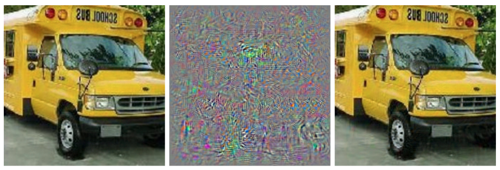
Figure 1: A school bus is classified as an ostrich after a small perturbation is applied to the original image (Szegedy et al.,, 2013).

As our work pertains to the robustness of machine learning algorithms to evasion attacks in classification tasks from a learning theory perspective, our review of related work will mainly concern this topic (Section 5.1). Before discussing this body of work, we will briefly mention other views on robustness.

Many works have studied the robustness of learning algorithms to poisoning attacks, in which an adversary can modify the training data in order to increase the (standard) error at test time, one of the earliest being that of Kearns and Li, (1988). Various types of poisoning attacks have been put forward since then, especially as the study of robustness has garnered interest in recent years. Clean-label attacks, proposed by Shafahi et al., (2018), are a distinct form of poisoning attacks where the poisoned examples are labelled correctly, i.e., by the target function, and not adversarially. For a learning-theoretic approach and results on this problem, see (Mahloujifar and Mahmoody,, 2017, 2019; Mahloujifar et al.,, 2018, 2019; Etesami et al.,, 2020; Blum et al.,, 2021) (non-exhaustive). In case there is no restriction on the label of poisoned data, see, e.g., the works of (Barreno et al.,, 2006; Biggio et al.,, 2012; Papernot et al.,, 2016; Steinhardt et al.,, 2017) (non-exhaustive). Finally, for work on defences against poisoning attacks, we refer the reader to (Goldblum et al.,, 2022).

Another view on robustness is out-of-distribution detection, where the goal is to identify outliers at test time. We refer the reader to the textbook (Quinonero-Candela et al.,, 2008) for an introduction on dataset shifts, and to (Fang et al.,, 2022) for a study on out-of-distribution detection from a PAC-learning perspective, as well as references therein for the empirical work on the matter. A more general view on distributional discrepancies at test-time is that of distribution shift. See (Wiles et al.,, 2022) for a taxonomy on various distribution shifts and a review of important work in the area (mostly from an empirical perspective).

5.1 Evasion Attacks

We now turn our attention to the focus of this thesis: robustness to evasion attacks. For ease of reading, we have thematically split the related work in this section.

Defining Robustness.

The majority of the guarantees and impossibility results for evasion attacks are based on the existence of adversarial examples. However, what is considered to be an adversarial example has been defined in different, and in some respects contradictory, ways in the literature. What we refer to as the exact-in-the-ball notion of robustness in this work (also known as error region risk in (Diochnos et al.,, 2018)) requires that the hypothesis and the ground truth agree in the perturbation region around each test point; the ground truth must thus be specified on all input points in the perturbation region. On the other hand, what we refer to as the constant-in-the-ball notion of robustness (which is also known as corrupted input robustness from the work of Feige et al., (2015)) requires that the unperturbed point be correctly classified and that the points in the perturbation region share its label, meaning that we only need access to the test point labels; the works Diochnos et al., (2018); Dreossi et al., (2019); Pydi and Jog, (2021) offer thorough discussions on the subject and also compare robustness definitions. Moreover, Chowdhury and Urner, (2022) have studied settings where a model’s change of label is justified by looking at robust-Bayes classifiers and their standard counterparts.

We note that Suggala et al., (2019) proposed an alternative definition of robustness, where a perturbation is deemed adversarial if it causes a label change in the hypothesis while the target classifier’s label remains constant. The existence of a ground truth is thus explicitly assumed (which is not in general necessary for constant-in-the-ball robustness).

Rather than studying the existence of a misclassification in the perturbation region, Pang et al., (2022) define robustness using the Kullback-Leibler (KL) divergence. The robust loss at a given unperturbed point $x$ is the maximal KL divergence over perturbations $z$ between the underlying labelling function ($\underset{{}}{\Pr}\left(y\;|\;z\right)$) of $z$ and the hypothesis’ label for $z$ (which could also be non-deterministic). The authors proposed this definition of robustness in an effort to avoid the trade-off between accuracy and robustness observed in prior work, e.g., (Tsipras et al.,, 2019).

In the remainder of this section, whenever the robust risk is not explicitly mentioned, the results will hold for the constant-in-the-ball notion of robustness, as it is the most widely used in the literature.

Existence of Adversarial Examples.

There is a considerable body of work that studies the inevitability of adversarial examples, e.g., (Fawzi et al.,, 2016; Fawzi et al., 2018a, ; Fawzi et al., 2018b, ; Gilmer et al.,, 2018; Shafahi et al.,, 2019; Tsipras et al.,, 2019). These papers characterize robustness in the sense that a classifier’s output on a point should not change if a perturbation of a certain magnitude is applied to it. These works also study geometrical characteristics of classifiers and statistical characteristics of classification data that lead to adversarial vulnerability. It has been shown that, in many instances, the vulnerability of learning models to adversarial examples is inevitable due to the nature of the learning problem. Notably, Bhagoji et al., (2019) study robustness to evasion attacks from an optimal transport perspective, obtaining lower bounds on the robust error. Moreover, many works exhibit a trade-off between standard accuracy and robustness in this setting, e.g., (Tsipras et al.,, 2019; Dobriban et al.,, 2020).

As for the exact-in-the-ball definition of robustness, Diochnos et al., (2018) consider the robustness of monotone conjunctions under the uniform distribution. Their results concern the ability of an adversary to magnify the missclassification error of any hypothesis with respect to any target function by perturbing the input. Mahloujifar et al., (2019) generalized the above-mentioned result to Normal Lévy families and a class of well-behaved classification problems (i.e., ones where the error regions are measurable and average distances exist).

Computational Complexity of Robust Learning.

The computational complexity of robust learning is an active research area. Bubeck et al., (2018) and Degwekar et al., (2019) have shown that there are concept classes that are hard to robustly learn under cryptographic assumptions, even when robust learning is information-theoretically feasible. (Bubeck et al.,, 2019) established super-polynomial lower bounds for robust learning in the statistical query framework. Diakonikolas et al., (2019) study the more specific problem of (standard) proper learning of halfspaces with noise and large $\ell_{2}$ margins in the agnostic PAC setting, focussing on the computational complexity of this learning problem. They remark that these guarantees can apply to robust learning. In follow-up work (Diakonikolas et al.,, 2020), they explicitly study robustness to $\ell_{2}$ perturbations and generalize their previous results. In particular, they obtain computationally-efficient algorithms using an online learning reduction, and building on a hardness result in (Diakonikolas et al.,, 2019), and provide tight running time lower bounds. Finally, Awasthi et al., (2019) draw connections between robustness to evasion attacks and polynomial optimization problems, obtaining a computational hardness result. On the other hand, they exhibit computationally efficient robust learning algorithms for linear and quadratic threshold functions in the realizable case.

Sample Complexity of Robust Learning.

Despite being a relatively recent research area, there already exists a vast literature on the sample complexity of robust learning to evasion attacks. One of the earlier works is that of Cullina et al., (2018), who define the notion of adversarial VC dimension to derive sample complexity upper bounds for robust empirical risk minimization (ERM) algorithms, with respect to the constant-in-the-ball robust risk. They also study the special case of halfspaces under $\ell_{p}$ perturbations and show the adversarial VC dimension is in general incomparable with its standard counterpart. Shortly after, Attias et al., (2019) adopted a game-theoretic framework to study robust learnability for classification and regression in a setting where the adversary is limited to a fixed number $k$ of perturbations per input. They obtain sample complexity bounds that are linear in both $k$ and the VC dimension of a hypothesis class. The work of Montasser et al., (2019) later provided a more complete picture of robust learnability. The authors show sample complexity upper bounds for robust ERM algorithms that are polynomial in the VC and dual VC dimensions of concept classes, giving general upper bounds that are exponential in the VC dimension. They also exhibit sample complexity lower bounds linear in the robust shattering dimension, a notion of complexity introduced therein. The gap between the upper and lower bounds was closed in their later work (Montasser et al.,, 2022), where they fully characterize the sample complexity of robust learning with arbitrary perturbation functions. The robust learning algorithm achieving the upper bound is a generalization of the one-inclusion graph algorithm of Haussler et al., (1994). Their robust variant of the one-inclusion graph is defined for the constant-in-the-ball realizable setting, but the agnostic-to-realizable reduction from previous work (Montasser et al.,, 2019) can be applied. The (random-example) sample complexity characterizing robust learnability is a notion of dimension defined through the edges on the graph structure.

The above bounds consider the supervised setting, where the learner has access to labelled examples. Since the cost of obtaining data is at times largely due to its labelling, studying semi-supervised learning, where the learner has access to both unlabelled as well as labelled examples, is of general interest. Ashtiani et al., (2020) build on the work of Montasser et al., (2019) (who showed that proper robust learning, where the learner is required to output a hypothesis from the same class as the potential target concept, is sometimes impossible) and delineate when proper robust learning is possible. They moreover draw a more nuanced picture of proper robust learnability with access to unlabelled random examples. Attias et al., (2022) also study the sample complexity of robust learning in the semi-supervised framework. Notably, in the realizable setting, their labelled sample complexity bounds are linear in a variant of the VC dimension where, for a shattered set, the perturbation region around a given point must share the same label. The unlabelled sample complexity is linear in the sample complexity of supervised learning. The authors also extend their results to the agnostic setting.

While it is worthwhile to study robust learnability for arbitrary perturbation regions, focussing on specific perturbation functions that are more faithful to real-world problems is of high interest, especially if this can provide better guarantees or a clearer picture of robustness in this setting. In this vein, Shao et al., (2022) study the robustness to evasion attacks under transformation invariances. This terminology comes from group theory: the transformations applied to instances form a group, and an invariant hypothesis will give the same label to points in the orbit of every instance in the support of the distribution generating the data. As a characterization of robust learnability in these settings, they propose two combinatorial measures that are variants of the VC dimension that take into account the orbits of points in the shattered set, and prove nearly-matching upper and lower bounds.

All the works mentioned above study sample complexity through the VC dimension of a concept class, or variants adapted to robust learnability. On the other hand, Khim et al., (2019); Yin et al., (2019); Awasthi et al., (2020) instead use the adversarial Rademacher complexity to study robust learning. These works give results for ERM on linear classifiers and neural networks.

As for the exact-in-the-ball definition of robustness, Diochnos et al., (2020) study sample complexity lower bounds. They show that, for a wide family of concept classes, any learning algorithm that is robust against all attacks with budget $\rho=o(n)$ must have a sample complexity that is at least exponential in the input dimension $n$. They also show a superpolynomial lower bound in case $\rho=\Theta(\sqrt{n})$. This, along with the previously-mentioned works of Diochnos et al., (2018); Mahloujifar et al., (2019) are to our knowledge the only other works apart from ours that consider the sample complexity of exact-in-the-ball robust learning from a theoretical perspective.

Relaxing Robustness Requirements.

Most adversarial learning guarantees and impossibility results in the literature have focused on all-powerful adversaries. Recent works have studied learning problems where the adversary’s power is curtailed. One way to do this is to consider computationally-bounded adversaries. E.g, Mahloujifar and Mahmoody, (2019) and Garg et al., (2020) study the robustness of classifiers to polynomial-time attacks. They show that, for product distributions, an initial constant error implies the existence of a (black-box) polynomial-time attack for adversarial examples that are $O(\sqrt{n})$ bits away from the test instances. However, Garg et al., (2020) show a separation result for a learning problem where a classifier can be successfully attacked by a computationally-unbounded adversary, but not by a polynomial-time bounded adversary subject to standard cryptographic hardness assumptions.

It is also possible to relax the optimality condition when evaluating a hypothesis. Ashtiani et al., (2023) and Bhattacharjee et al., (2023) both study tolerant robust learning, where the learner is evaluated relative to the hypothesis with the best robust risk under a slightly larger perturbation region. Ashtiani et al., (2023) show that this setting enables better sample complexity bounds that the standard robust setting for metric spaces $(\mathcal{X},d)$ in case the perturbation region is a ball with respect to the metric $d$. Bhattacharjee et al., (2023) build on their work and instead consider problems with a geometric niceness property called regularity to get more general perturbation regions. They obtain matching sample complexity bounds to (Ashtiani et al.,, 2023) as well as propose a variant of robust ERM as a simpler robust learning algorithm for this problem.

Another relaxation of the robust learning objective is a probabilistic variant of robust learning. Viallard et al., (2021) derive PAC-Bayesian generalization bounds (where the output is a posterior distribution over hypotheses after seeing the data) for the averaged risk on the perturbations, rather than working in a worst-case scenario. (Robey et al.,, 2022) also consider probabilistic robustness, where the aim is to output a hypothesis that is robust to most perturbations.

Increasing the Learner’s Power.

To improve robustness guarantees, it is also possible to give the learner access to more powerful oracles than the random-example one. Montasser et al., (2020, 2021) study robust learning with access to a (constant-in-the-ball) robust loss oracle, which they call the Perfect Attack Oracle (PAO). For a perturbation type $\mathcal{U}:\mathcal{X}\rightarrow 2^{\mathcal{X}}$, hypothesis $h$ and labelled point $(x,y)$, the PAO returns the constant-in-the-ball robust loss of $h$ in the perturbation region $\mathcal{U}(x)$ and a counterexample $z\in\mathcal{U}(x)$ where $h(z)\neq y$ if it exists. In the constant-in-the-ball realizable setting, the authors use online learning results to show sample and query complexity bounds that are linear and quadratic in the Littlestone dimension of concept classes, respectively (Montasser et al.,, 2020). Montasser et al., (2021) moreover use the algorithm from (Montasser et al.,, 2019) to get sample and query complexity upper bounds that respectively have a linear and exponential dependence on the VC and dual VC dimensions of the hypothesis class at hand. Finally, they extend their results to the agnostic setting and derive lower bounds.

Chapter 3 Background

In this chapter, we introduce the necessary background and notation for the main contributions of this thesis. We start by reviewing standard learning theory concepts in Section 6, before moving to probability theory in Section 7. We finish with an overview of Fourier analysis in Section 8.

Notation.

Throughout this text, we will use $[n]$ to denote the set $\left\{1,\dots,n\right\}$. The symbol $\Delta$ will represent the symmetric difference between two sets: $I\Delta J=\left\{x\;|\;x\in I\setminus J\text{ or }x\in J\setminus I\right\}$. We will use the asymptotic notation ($o,O,\omega,\Omega,\Theta$), with the convention that the symbol $\;\widetilde{\;}$ (e.g., $\widetilde{O}$) omits the logarithmic factors. Given a metric space $(\mathcal{X},d)$ and $\lambda\in\mathbb{R}$, we denote by $B_{\lambda}(x)$ the ball $\left\{z\in\mathcal{X}\;|\;d(x,z)\leq\lambda\right\}$ of radius $\lambda$ centred at $x$. We will use the symbol $\mathbf{1}[\cdot]$ for the indicator function. Finally, for a given formula $\varphi$ and instance $x$, we denote by $x\models\varphi$ the event that $x$ satisfies $\varphi$.

6 Learning Theory: Classification

Learning theory offers an elegant abstract framework to analyse the behaviour of machine learning algorithms, as well as to provide performance and correctness guarantees or show impossibility results. There exist various learning settings, depending on assumptions on how the data is obtained and on the learning objectives. This thesis is primarily concerned with binary classification, where, given an input space $\mathcal{X}$, the goal is to output a function $h:\mathcal{X}\rightarrow\{0,1\}$ called a hypothesis, which upon being given an instance $x\in\mathcal{X}$ outputs a label $h(x)\in\{0,1\}$. The more general task of learning a function $\mathcal{X}\rightarrow\mathcal{Y}$ is called multiclass classification when $\mathcal{Y}$ is a discrete finite set, and regression when $\mathcal{Y}=\mathbb{R}$.

In this section, we give an overview of three learning settings for binary classification: learning with random examples in the Probably Approximately Correct (PAC) framework, the mistake-bound model of online learning, and learning with membership and equivalence queries. For each setting, we discuss various notions of complexity that control the amount of data needed to learn, i.e., the sample complexity. In all cases, we will be using the terms learning algorithm, learner and learning process interchangeably to denote a process of data acquisition and analysis resulting in outputting a hypothesis $h$ as above. For a more in-depth introduction to the concepts presented in this section, we refer the reader to Mohri et al., (2012) and Shalev-Shwartz and Ben-David, (2014), both excellent introductory textbooks on learning theory.

6.1 The PAC Framework

The Probably Approximately Correct (PAC) framework of Valiant, (1984), depicted in Figure 2, formalises the desired behaviour of a learning algorithm. In this learning setting, a learning algorithm has access to random examples drawn in an i.i.d. fashion from an underlying distribution $D$, and we wish to output a hypothesis that has small error with high confidence. The error $\text{err}_{D}(h,c)$ of a hypothesis with respect to $D$ is measured against a ground truth function or target concept $c:\mathcal{X}\rightarrow\{0,1\}$ which labels the data, and is defined as

$$\text{err}_{D}(h,c)=\underset{{x\sim D}}{\Pr}\left(c(x)\neq h(x)\right)\enspace.$$

The set of points $x\in\mathcal{X}$ such that $c(x)\neq h(x)$ is often referred to as the error region. We sometimes model the sampling process by having access to the random example oracle $\mathsf{EX}(c,D)$. The “probably” part of the PAC learning framework speaks to the confidence of the learning algorithm, and allows for the possibility that a sample $S\sim D^{m}$ of size $m$ drawn from the underlying distribution $D$ is not representative of $D$. The “approximately” part of PAC learning refers to the requirement that the hypothesis have sufficiently high accuracy, a relaxation from learning exactly. Both the confidence and accuracy parameters are inputs to the learning algorithm, and are learning parameters.

Another important parameter that affects the sample complexity is how large the instance size is, e.g., the larger the number of pixels for image classification is, the larger the amount of data needed to learn could be. This is usually controlled by the dimension $n$ of the input space, in reference to $\left\{0,1\right\}^{n}$ and $\mathbb{R}^{n}$. To this end we consider a collection of pairs of input space and concepts classes $\mathcal{X}_{n}$ and $\mathcal{C}_{n}$ for each dimension $n$, where $\mathcal{C}_{n}$ is a set of functions $c:\mathcal{X}_{n}\rightarrow\{0,1\}$.

We are now ready to formally define the PAC learning setting.

Definition 3.1 (PAC Learning, Realizable Setting).

For all $n\in\mathbb{N}$, let $\mathcal{C}_{n}$ be a concept class over $\mathcal{X}_{n}$ and let $\mathcal{C}=\bigcup_{n\in\mathbb{N}}\mathcal{C}_{n}$. We say that $\mathcal{C}$ is PAC learnable using hypothesis class $\mathcal{H}$ and sample complexity function $m(\cdot,\cdot,\cdot,\cdot)$ if there exists an algorithm $\mathcal{A}$ that satisfies the following: for all $n\in\mathbb{N}$, for every $c\in\mathcal{C}_{n}$, for every $D$ over $\mathcal{X}_{n}$, for every $0<\epsilon<1/2$ and $0<\delta<1/2$, if whenever $\mathcal{A}$ is given access to $m\geq m(n,1/\epsilon,1/\delta,\text{size}(c))$ examples drawn i.i.d. from $D$ and labeled with $c$, $\mathcal{A}$ outputs an $h\in\mathcal{H}$ such that with probability at least $1-\delta$,

$$\text{err}_{D}(h,c)=\underset{{x\sim D}}{\Pr}\left(c(x)\neq h(x)\right)\leq\epsilon\enspace.$$

We say that $\mathcal{C}$ is statistically efficiently PAC learnable if $m$ is polynomial in $n,1/\epsilon$, $1/\delta$ and size$(c)$, and computationally efficiently PAC learnable if $\mathcal{A}$ runs in polynomial time in $n,1/\epsilon$, $1/\delta$ and size$(c)$ and $h$ is polynomially evaluatable.

Probably Approximately Correct Learning

Figure 2: A visual representation of sample-efficient PAC learning. $S_{c}$ means that the sample $S$ has been labelled with the ground truth $c$.

Size$(c)$ and polynomial evaluatability.

Two additional requirements from accuracy and confidence are introduced in the above definition: these are a sample complexity function dependent on the size $size(c)$ of the target concept $c$, and, if one requires computational efficiency, the fact that $h$ is polynomially evaluatable. The size of a concept is defined through a representation scheme. Essentially, there could exist several representations of a function, e.g., a function can be computed by many different boolean circuits. Assuming that there exists a function measuring the size of a representation, the size of a concept $c$ is the minimal size of a representation of $c$. The second requirement is natural: if the hypothesis is not required to be polynomially evaluatable, then the learner could simply “offload” the learning process at test time (there is nothing to do at training, so it would be considered “efficient”), and overall require arbitrarily high computational complexity.

Proper vs improper learning.

The setting where $\mathcal{C}=\mathcal{H}$ is called proper learning, and improper learning if $\mathcal{C}\subseteq\mathcal{H}$. While requiring proper learning does not affect the sample complexity of learning very much, it can affect its computational efficiency. Indeed, unless $\mathsf{RP}=\mathsf{NP}$, which is widely believed not to be the case, it is impossible to computationally efficiently properly learn the class of 3-term formulas in disjunctive normal form (DNF), i.e., formulas of the form $T_{1}\vee T_{2}\vee T_{3}$ where the $T_{i}$’s are conjunctions of arbitrary lengths. However, it is possible to computationally efficiently PAC learn 3-CNF formulas properly (formulas in conjunctive normal form where each term is a disjunction of at most 3 literals), and this class subsumes 3-term DNFs. Hence, one can use the PAC-learning algorithm for 3-CNF to (improperly) PAC learn 3-term DNFs in a computationally efficient manner.

The distribution-free assumption.

PAC learning is distribution-free, in the sense that no assumptions are made about the distribution from which the data is generated. As long as the training data is sampled i.i.d. from a given distribution $D$, and that the algorithm is tested on independent examples drawn from $D$, the learning guarantees hold. Of course, this is sometimes not a sensible assumption to make in practice. Many lines of work consider learning settings that allow for this and provide a more realistic learning framework, e.g., when noise is added to the data, or when the training and testing distributions differ (i.e., distribution shift), as outlined in Chapter 2.

Realizable vs agnostic learning.

The realizability assumption of Definition 3.1, where there always exists a concept with zero error, does not always hold. In the presence of noise, or more generally in the absence of a deterministic labelling function $c$ representing the ground truth (e.g., there is a joint distribution on $\mathcal{X}\times\mathcal{Y}$), we instead work in the agnostic setting. In this setting, the goal is rather to learn a hypothesis that does well compared to the best concept in the concept class:

Definition 3.2 (PAC Learning, Agnostic Setting).

Let $\mathcal{C}_{n}$ be a concept class over $\mathcal{X}_{n}$ and let $\mathcal{C}=\bigcup_{n\in\mathbb{N}}\mathcal{C}_{n}$. We say that $\mathcal{C}$ is agnostically PAC learnable using $\mathcal{H}$ with sample complexity function $m(\cdot,\cdot,\cdot,\cdot)$ if there exists an algorithm $\mathcal{A}$ that satisfies the following: for all $n\in\mathbb{N}$, for every $D$ over $\mathcal{X}_{n}\times\{0,1\}$, for every $0<\epsilon<1/2$ and $0<\delta<1/2$, if whenever $\mathcal{A}$ is given access to $m\geq m(n,1/\epsilon,1/\delta,s)$ labelled examples drawn i.i.d. from $D$, where $s=\underset{c\in\mathcal{C}_{n}}{\sup}\;\text{size(c)}$, $\mathcal{A}$ outputs an $h\in\mathcal{H}$ such that with probability at least $1-\delta$,

$$\text{err}_{D}(h)\leq\underset{c\in\mathcal{C}_{n}}{\inf}\text{err}_{D}(c)+\epsilon\enspace,$$

where $\text{err}_{D}(h)=\underset{{(x,y)\sim D}}{\Pr}\left(h(x)\neq y\right)$. We say that $\mathcal{H}$ is statistically efficiently agnostically learnable if $m$ is polynomial in $n,1/\epsilon$, $1/\delta$ and $s$, and computationally efficiently agnostically learnable if $\mathcal{A}$ runs in polynomial time in $n,1/\epsilon$, $1/\delta$ and $s$, and $h$ is polynomially evaluatable.

The definition above allows for improper learning ($\mathcal{C}$ is usually called the “touchstone” class), but we can recover proper learning by setting $\mathcal{C}=\mathcal{H}$. In this work, unless otherwise stated, we will assume the realizability of a learning problem, and the sample complexity bounds will be derived for this setting. Note that there exist PAC guarantees for classes of finite VC dimension in the agnostic setting as well, at the cost of a multiplicative factor of $1/\epsilon$ in the sample complexity. See (Kearns et al.,, 1994; Haussler,, 1992) for original work on the matter and the textbook (Mohri et al.,, 2012) for an introduction on the topic.

6.2 Complexity Measures

While it is possible to derive sample complexity bounds for specific hypothesis classes, one can take a more general approach with the use of complexity measures. Indeed, a complexity measure assigns to each hypothesis class $\mathcal{H}$ a function (w.r.t. the size $n$ of the instance space) quantifying its richness. Intuitively, as the complexity measure increases, more data should be needed to identify a candidate hypothesis that would generalize well on unseen data. We briefly note that the standard theory outlined in this chapter has failed to explain the recent success of overparametrised deep neural networks in practice which in many ways remains an open problem in the learning theory literature.

The first complexity measure we will study is perhaps the simplest one: the size of $\mathcal{H}$. Similarly to $\mathcal{C}$, the class $\mathcal{H}$ is defined as the union $\bigcup_{n\in\mathbb{N}}\mathcal{H}_{n}$, and the size of $\mathcal{H}$ is a function of $n$. The theorem below, known as Occam’s razor, gives an upper bound on the sample complexity of learning with finite hypothesis classes, given access to a consistent learner. A consistent learner is a learning algorithm that outputs a hypothesis that has zero empirical loss on the training sample, i.e., a hypothesis that correctly classifies all the points in the training sample.

Theorem 3.3 (Occam’s Razor (Blumer et al.,, 1987)).

Let $\mathcal{C}$ and $\mathcal{H}$ be a concept and hypothesis classes, respectively. Let $\mathcal{A}$ be a consistent learner for $\mathcal{C}$ using $\mathcal{H}$. Then, for all $n\in\mathbb{N}$, for every $c\in\mathcal{C}_{n}$, for every $D$ over $\mathcal{X}_{n}$, for every $0<\epsilon<1/2$ and $0<\delta<1/2$, if whenever $\mathcal{A}$ is given access to $m\geq\frac{1}{\epsilon}\left(\log(|\mathcal{H}_{n}|)+\log(1/\delta)\right)$ examples drawn i.i.d. from $D$ and labeled with $c$, then $\mathcal{A}$ is guaranteed to output an $h\in\mathcal{H}_{n}$ such that $\text{err}_{D}(h,c)<\epsilon$ with probability at least $1-\delta$. Furthermore, if $\log(|\mathcal{H}_{n}|)$ is polynomial in $n$ and size$(c)$, and $h$ is polynomially evaluatable, then $\mathcal{C}$ is statistically efficiently PAC-learnable using $\mathcal{H}$.

While the theorem above can be useful if $\mathcal{H}_{n}$ is finite for all $n$, it does not tell us much when $\mathcal{H}$ is infinite. To this end, one would want to consider complexity measures that are meaningful for infinite concept classes as well. In the PAC setting, a useful complexity measure is the Vapnik Chervonenkis (VC) dimension of a hypothesis class, from the work of Vapnik and Chervonenkis, (1971). It turns out that this measure fully characterizes the learnability of a concept class, in the sense that one can obtain upper and lower bounds on the sample complexity that are both linear in the VC dimension of $\mathcal{H}$.

In order to define the VC dimension of a concept class, we must first define the notion of shattering of a set. In Figure 3, we give an example of a set being shattered by linear classifiers in $\mathbb{R}^{2}$.

Definition 3.4 (Shattering).

Given a class of functions $\mathcal{F}$ from input space $\mathcal{X}$ to $\left\{0,1\right\}$, we say that a set $S\subseteq\mathcal{X}$ is shattered by $\mathcal{F}$ if all the possible dichotomies of $S$ (i.e., all the possible ways of labelling the points in $S$) can be realized by some $f\in\mathcal{F}$.

(a)

(b)

(c)

(d)

Figure 3: A set $X$ of three points in $\mathbb{R}^{2}$ that is shattered by linear classifiers. Subfigures (a)-(d) represent different dichotomies on $X$; note that (b) and (c) are not the only labellings with one and two positively labelled points, respectively, but the other cases are symmetric.

We are now ready to define the VC dimension of a class.

Definition 3.5 (VC Dimension).

The VC dimension of a hypothesis class $\mathcal{H}$, denoted $\mathsf{VC}(\mathcal{H})$, is the size $d$ of the largest set that can be shattered by $\mathcal{H}$. If no such $d$ exists then $\mathsf{VC}(\mathcal{H})=\infty$.

Figure 4 illustrates the argument that no set in $\mathbb{R}^{2}$ of size 4 can be shattered by linear classifiers.

An important property of the VC dimension is that it is upper bounded by $\log\left|\mathcal{H}\right|$. Indeed, a shattered set $S$ of size $m$ needs $2^{m}$ distinct functions to achieve all its possible labellings.

It also is possible to define the VC dimension through the growth function of a concept class. For some finite set of instances $S$, we denote by $\Pi_{\mathcal{C}}(S)=\{c|_{S}\;|\;c\in\mathcal{C}\}$ the set of distinct restrictions of concepts in $\mathcal{C}$ on the set $S$, which is referred to as the set of all possible dichotomies on $S$ induced by $\mathcal{C}$. Then a shattered set $S$ satisfies $\left|\Pi_{\mathcal{C}}(S)\right|=2^{\left|S\right|}$, and the VC dimension is thus the largest set satisfying this relationship.

(a)

(b)

Figure 4: Any set of four points cannot be shattered by linear classifiers. Indeed, we distinguish two cases: either (a) one point is strictly in the convex hull of the three other points, and is the only point of its label (or all points are on the same line, which gives a similar argument) or (b) all points are on the boundary of the convex hull, in which case labelling opposite points with the same label gives an unachievable labelling. This argument is a special case for $\mathbb{R}^{2}$ which can be generalized to $\mathbb{R}^{n}$ using Radon’s theorem.

Definition 3.6 (Growth Function).

For any natural number $m\in\mathbb{N}$, the growth function is defined as $\Pi_{\mathcal{C}}(m)=\max\left\{\left|\Pi_{\mathcal{C}}(S)\right|\;|\;\left|S\right|=m\right\}$.

Denote by $\Phi_{d}(m)$ the summation $\sum_{i=0}^{d}{m\choose i}$. The growth function of a concept class $\mathcal{C}$ can be bounded as follows, as a function of $m$ and the VC dimension $d$.

Lemma 3.7 (Sauer-Shelah).

Let $\mathcal{C}$ be a concept class of VC dimension $d$. Then

$$\Pi_{\mathcal{C}}(m)\leq\Phi_{d}(m)\leq\left(\frac{em}{d}\right)^{d}\enspace.$$

As previously mentioned, the VC dimension characterizes PAC learnability. We start with a sample complexity upper bound that is linear in the VC dimension, due to Vapnik, (1982) and Blumer et al., (1989).

Theorem 3.8 (VC Dimension Sample Complexity Upper Bound).

Let $\mathcal{C}$ be a concept class. Let $\mathcal{A}$ be a consistent learner for $\mathcal{C}$ using a hypothesis class $\mathcal{H}$ of VC dimension $\mathsf{VC}(\mathcal{H})=d$. Then $\mathcal{A}$ is a PAC-learning algorithm for $\mathcal{C}$ using $\mathcal{H}$ provided it is given an i.i.d. sample $S\sim D^{m}$ drawn from some $D$ and labelled with some $c\in\mathcal{C}$, where

$$m\geq\kappa_{0}\cdot\frac{1}{\epsilon}\left(d\log\frac{1}{\epsilon}+\log\frac{1}{\delta}\right)\enspace,$$

for some universal constant $\kappa_{0}$.

We now have a sample complexity lower bound that is also linear in the VC dimension, due to Blumer et al., (1989) and Ehrenfeucht et al., (1989). The proofs of both Theorems 3.8 and 3.9 appear in reference textbooks such as (Mohri et al.,, 2012) and (Shalev-Shwartz and Ben-David,, 2014).

Theorem 3.9 (VC Dimension Sample Complexity Lower Bound).

Let $\mathcal{C}$ be a concept class with VC dimension $d$. Then any PAC-learning algorithm for $\mathcal{C}$ requires $\Omega\left(\frac{d}{\epsilon}+\frac{1}{\epsilon}\log\frac{1}{\delta}\right)$ examples.

While the bounds of Theorems 3.8 and 3.9 are tight up to a $\log\frac{1}{\epsilon}$, the breakthrough work of Hanneke, (2016) recently showed the existence of a specific learning algorithm that is optimal in the sense that its sample complexity matches that of Theorem 3.9 up to constant factors, and thus avoids the $\log\frac{1}{\epsilon}$ dependence.

6.3 Some Concept Classes and PAC Learning Algorithms

In this section, we introduce various concept classes that have been studied in the learning theory literature, along with PAC learning algorithms. All the algorithms outlined below are consistent on a given training sample, given we are working in the realizable setting. A bound on the VC dimension of these concept classes directly gives sample complexity upper bounds as per Theorem 3.8. We start with concept classes defined on the boolean hypercube $\mathcal{X}=\left\{0,1\right\}^{n}$.

Singletons.

For an input space $\mathcal{X}$, the class of singletons is the class of functions $\left\{x\mapsto\mathbf{1}[x=x^{*}]\;|\;x^{*}\in\mathcal{X}\right\}$.

Dictators.

The class of dictators on $\left\{0,1\right\}^{n}$ is the class of functions determined by a single bit, i.e., functions of the form $h(x)=x_{i}$ or $h(x)=\bar{x_{i}}$ for $i\in[n]$. Dictators are subsumed by conjunctions. Monotone dictators are dictators where negations are not allowed, i.e., functions of the form $h(x)=x_{i}$.

Conjunctions.

Conjunctions, which we denote CONJUNCTIONS, are perhaps one of the simplest non-trivial concept classes one can study on the boolean hypercube. A conjunction $c$ over $\{0,1\}^{n}$ is a logical formula over a set of literals $l_{1},\dots,l_{k}$ from $\left\{x_{1},\bar{x_{1}},\dots,x_{n},\bar{x_{n}}\right\}$, where, for $x\in\mathcal{X}_{n}$, $c(x)=\bigwedge_{i=1}^{k}l_{i}$. The length of a conjunction $c$ is the number of literals in $c$. For example, $c(x)=x_{1}\wedge\bar{x_{2}}\wedge{x_{5}}$ is a conjunction of length 3. Monotone conjunctions are the subclass of conjunctions where negations are not allowed, i.e., all literals are of the form $l_{i}=x_{j}$ for some $j\in[n]$. Note that this implies that monotone conjunctions do not include the constant function 0.

Algorithm 1 PAC-learning algorithm for conjunctions

$S_{c}\sim D^{m}$

$L\leftarrow\left\{x_{1},\bar{x_{1}},\dots,x_{n},\bar{x_{n}}\right\}$

$h(x)=\bigwedge_{l\in L}l$ $\triangleright$ $h=0$

for $(x,c(x))\in S$ do

     if $c(x)\neq h(x)$ then $\triangleright$ Only happens if $c(x)=1$

         $L\leftarrow L\setminus\left\{l\in L\;|\;l(x)=0\right\}$

     end if

end for

The standard PAC learning algorithm to learn conjunctions is as outlined in Algorithm 1. We start with the constant hypothesis $h(x)=\bigwedge_{i\in I_{h}}(x_{i}\wedge\bar{x_{i}})\equiv 0$, where $I_{h}=[n]$. To ensure consistency, for each example $x$ in the training sample, we remove a literal $l$ from $h$ if $c(x)=1$ and $l(x)=0$, as if $l$ is in the conjunction, $h$ must evaluate to $0$ on $x$. After seeing all the examples in the training set $S$, the resulting hypothesis will thus be consistent on $S$. Note that $\mathsf{VC}(\textsf{CONJUNCTIONS}_{n})=n$ (Natschläger and Schmitt,, 1996). Finally, Algorithm 1 can also be used for monotone conjunctions, but where the initial hypothesis is $h(x)=\bigwedge_{i\in[n]}x_{i}$.

CNF and DNF formulas.

A formula $\varphi$ in the conjunctive normal form (CNF) is a conjunction of clauses, where each clause is itself a disjunction of literals. A $k$-CNF formula is a CNF formula where each clause contains at most $k$ literals. For example, $\varphi=(x_{1}\vee x_{2})\wedge(\bar{x_{3}}\vee x_{4})\wedge\bar{x_{5}}$ is a 2-CNF. On the other hand, a DNF formula is a disjunction of clauses, where each clause is itself a conjunction of literals. A $k$-DNF is defined analogously to a $k$-CNF.

Decision lists.

Given a positive integer $k$, a $k$-decision list $f\in k$-$\mathsf{DL}$ is a list $(K_{1},v_{1}),\dots,(K_{r},v_{r})$ of pairs where $K_{j}$ is a term in the set of all conjunctions of size at most $k$ with literals drawn from $\left\{x_{1},\bar{x_{1}},\dots,x_{n},\bar{x_{n}}\right\}$, $v_{j}$ is a value in $\left\{0,1\right\}$, and $K_{r}$ is $\mathtt{true}$. The output $f(x)$ of $f$ on $x\in\left\{0,1\right\}^{n}$ is $v_{j}$, where $j$ is the least index such that the conjunction $K_{j}$ evaluates to $\mathtt{true}$ on $x$. Decision lists subsume conjunctions. Indeed, a conjunction $c(x)=\bigwedge_{i=1}^{k}l_{i}$ can be expressed as the following 1-decision list: $(\neg l_{1},0),\dots,(\neg l_{k},0),(\mathtt{true},1)$.

The PAC-learning algorithm for decision lists, introduced by Rivest, (1987), is outlined in Algorithm 2. The sample size $m$ is given by Theorem 3.8 and an observation that the size of the class is $O\left(3^{\left|C_{n,k}\right|}\left|C_{n,k}\right|!\right)$, where $C_{n,k}$ is the set of conjunctions of length at most $k$ on $n$ variables, giving a VC dimension bound of $O(n^{k}\log n)$. Note that, as we consider $k$ to be a fixed constant, the sample complexity bound is polynomial in $n$ and the learning parameters.

Algorithm 2 PAC-learning algorithm for 1-decision lists from Rivest, (1987)

$S\sim D^{m}$

$L:=\left\{x_{i},\bar{x_{i}}\right\}_{i=1}^{n}$ $\triangleright$ Set of all literals

$h=\emptyset$ $\triangleright$ Empty decision list

while $S\neq\emptyset$ do

     if $\exists b\in\left\{0,1\right\}$ s.t. $\forall(x,y)\in S,\;y=b$ then

         $S\leftarrow\emptyset$

         append $(\mathtt{true},b)$ to $h$

     else

         for $l\in L$ s.t. $\exists(x,y)\in S$ s.t. $l(x)=1$ do $\triangleright$ $l$ is true for some $x$

              if $\exists b\in\left\{0,1\right\}$ s.t. $\forall(x,y)\in S\;\left(l(x)=1\Rightarrow y=b\right)$ then

                  append $(l,b)$ to $h$

                  $S\leftarrow S\setminus\left\{(x,y)\in S\;|\;l(x)=1\right\}$

              end if

         end for

     end if

end while

Note that, while the algorithm above is for 1-decision lists, it is sufficient to only consider this case. Indeed, if we are dealing with $k$-decision lists, we can draw our attention to the set $C_{n,k}$ of conjunctions of length at most $k$ on $n$ variables by defining the following injective map:

$$\Phi:\left\{0,1\right\}^{n}\rightarrow\left\{0,1\right\}^{C_{n,k}}\enspace,$$ (1)

where $\Phi(x)_{c_{i}}=\mathbf{1}[x\models c_{i}]$ for $c_{i}\in C_{n,k}$, i.e. whether $x$ satisfies clause $c_{i}$. Now, any distribution $D$ on $\left\{0,1\right\}^{n}$ induces a well-defined distribution $D^{\prime}$ on $\left\{0,1\right\}^{C_{n,k}}$. Moreover, since $\left|{C_{n,k}}\right|=O(n^{k})$, an input $x\in\left\{0,1\right\}^{n}$ and a 1-decision $h$ on $\left\{0,1\right\}^{n}$ can respectively be transformed into $\Phi(x)\in\left\{0,1\right\}^{C_{n,k}}$ and a $k$-decision list $h^{\prime}$ on $\left\{0,1\right\}^{C_{n,k}}$ in polynomial time, for a fixed $k$, and vice-versa in the case of going from $h^{\prime}$ to $h$. It also follows that $\text{err}_{D}(h,c)=\text{err}_{D^{\prime}}(h^{\prime},c^{\prime})$, where $c^{\prime}$ is the $k$-decision list on $\left\{0,1\right\}^{C_{n,k}}$ induced by $c$. Hence, an efficient learning algorithm for 1-decision lists can be used as a black box to efficiently learn $k$-decision lists.

Finally, the class of $k$-decision lists subsume $k$-CNF and $k$-DNF (Rivest,, 1987).

Decision trees.

A decision tree $T$ is a binary tree whose nodes are positive literals in $\left\{x_{1},\dots,x_{n}\right\}$. For a given node with variable $x_{i}$, the edge to its left child node is labelled with 0 and the edge to its right child node is labelled as 1, representing the value of the $x_{i}$ for a given instance $x\in\left\{0,1\right\}^{n}$. The leaves take label in $\left\{0,1\right\}$; a given $x\in\left\{0,1\right\}^{n}$ induces a path from the root to a leaf in $T$, which will give the label $T(x)$. Decision trees generalize 1-decision lists: a 1-decision list is a decision tree with each node having at most one child. Note that it is currently unknown whether polynomial-sized decision trees are PAC learnable.

Parities.

Parities are defined with respect to a subset $I\subseteq[n]$ of indices as $f_{I}(x)=\left(\sum_{i\in I}x_{i}\right)\bmod 2$, i.e. the output is whether adding the bits at indices in $S$ results in an odd or even sum. Learning parities amounts to learning the set $S$. Given a set of examples $(X,Y)\subseteq\left\{0,1\right\}^{n}\times\left\{0,1\right\}$, where each $(x,y)\in(X,Y)$ is a labelled example, finding this set is equivalent to finding a solution $a\in\left\{0,1\right\}^{n}$ to the system of linear equations $Xa=Y$ in the finite field $\mathbb{F}_{2}$. The set $J:=\left\{j\in[n]\;|\;a_{j}=1\right\}$ gives a hypothesis $f_{J}(x)=\left(\sum_{j\in J}x_{j}\right)\bmod 2$ consistent with the data. This can be done using Gaussian elimination, provided a solution exists (this is guaranteed by the realizability assumption). See (Helmbold et al.,, 1992; Goldberg,, 2006) for details.

Note that, when working in $\left\{-1,1\right\}^{n}$ instead of $\left\{0,1\right\}^{n}$, we can define the parity function as $f_{I}(x)=\prod_{i\in I}x_{i}$ instead. This representation will be especially relevant in Section 8 when we introduce Fourier analysis concepts.

Majorities.

Similarly to parities, majorities are defined with respect to a set $I$ of indices, as follows: $\text{maj}_{I}(x)=\mathbf{1}\left[\sum_{i\in I}x_{i}\geq\left|I\right|/2\right]$. Again, when working in $\left\{-1,1\right\}^{n}$ instead of $\left\{0,1\right\}^{n}$, majority functions are defined as $\text{maj}_{I}(x)=\text{sgn}\left(\sum_{i\in I}x_{i}\right)$. Clearly, from the representations above, majorities are subsumed by linear classifiers, which are defined further below.

Linear classifiers.

The class of linear classifiers (also known as halfspaces and linear threshold functions) on input spaces $\mathcal{X}=\left\{0,1\right\}^{n}$ or $\mathcal{X}=\mathbb{R}^{n}$ are defined as $\left\{x\mapsto\text{sgn}\left(w\cdot x+b\right)\;|\;w\in\mathbb{R}^{n},b\in\mathbb{R}\right\}$, where the $w_{i}\in w$ are the weights and $b$ is the bias. When the instance space is the reals, we will denote the class as $\mathsf{LTF}_{\mathbb{R}^{n}}$. Moreover, we will denote by $\mathsf{LTF}_{\left\{0,1\right\}^{n}}^{W}$ the class of linear threshold functions on $\left\{0,1\right\}^{n}$ with integer weights such that the sum of the absolute values of the weights and the bias is bounded above by $W$, and $W^{+}$ when the weights are positive. Finally, when the weights and the bias are binary, i.e., $w_{i},b\in\{0,1\}$ for all $i$, the class is called boolean threshold functions.

The VC dimension of halfspaces is $n+1$. The upper bound of $n+1$ can be shown by using Radon’s theorem (any set of size $n+2$ in $\mathbb{R}^{n}$ can be partitioned into two subsets whose convex hulls intersect), and the lower bound can be obtained by showing that the set $\left\{\mathbf{e}_{i}\right\}_{i=1}^{n}\cup\mathbf{0}$ can be shattered. The support vector machine (SVM) algorithm, or solving a system of linear inequalities with linear programming, can be used as a consistent learner for this concept class. Finally, the class of conjunctions is subsumed by linear classifiers: a conjunction $f(x)=\bigwedge_{i=1}^{k}l_{i}$ can be represented as the linear classifier $g(x)=\text{sgn}\left(\sum_{i\in I^{+}}x_{i}-\sum_{i\in I^{-}}x_{i}-\left|I\right|+1\right)$, where $I^{+}=\left\{j\in[n]\;|\;\exists i\;.\;l_{i}=x_{j}\right\}$ and $I^{-}=\left\{j\in[n]\;|\;\exists i\;.\;l_{i}=\bar{x_{i}}\right\}$.

6.4 Online Learning: The Mistake-Bound Model

In online learning, the learner is given access to examples sequentially. At each time step $t$, the learner receives an example $x_{t}$, predicts its label $\hat{y}_{t}$ using a given hypothesis class $\mathcal{H}$, receives the true label $y_{t}$ and can update its hypothesis, typically when $\hat{y}_{t}\neq y_{t}$. A fundamental distinction between the PAC- and online-learning models is that, in the latter, there are usually no distributional assumptions on the data. Thus, we need to evaluate the learner’s performance with different benchmark than the error $\text{err}_{D}(h)$ from the (offline) PAC setting.

In the mistake-bound model, examples and their labels can be given in an adversarial fashion. The performance of the learner is evaluated with respect to the number of mistakes it makes compared to the ground truth; we again assume the realizability of the learning problem, meaning that there is a target concept $c\in\mathcal{C}$ such that $c(x_{t})=y_{t}$ for all $t$. Crucially, the target concept need not be chosen a priori: the only requirement is that, at every time $t$, there exists a concept $c\in\mathcal{C}$ that is consistent on the past sequence of points $(x_{1},y_{1}),\dots,(x_{t},y_{t})$. The goal of the learner is to learn the target exactly.

We now formally define the mistake-bound model of online learning.

Definition 3.10 (Mistake Bound).

For a given hypothesis class $\mathcal{C}$ and instance space $\mathcal{X}=\bigcup_{n}\mathcal{X}_{n}$, we say that an algorithm $\mathcal{A}$ learns $\mathcal{C}$ with mistake bound $M$ if $\mathcal{A}$ makes at most $M$ mistakes on any sequence of samples consistent with a concept $c\in\mathcal{C}$.

In the mistake bound model, we usually require that $M$ be polynomial in $n$ and size$(c)$. A good example where this holds is the online learning algorithm for conjunctions, outlined in Algorithm 3, which is immediately adapted from its PAC-learning counterpart. Indeed, Algorithm 1 only changes its hypothesis whenever it sees a positive example $(x,1)$ such that $h(x)=0$, and works through the sample sequentially.

Algorithm 3 PAC-learning algorithm for conjunctions, online version

$L\leftarrow\left\{x_{1},\bar{x_{1}},\dots,x_{n},\bar{x_{n}}\right\}$

$h(x)=\bigwedge_{l\in L}l$ $\triangleright$ $h=0$

for $t=1,2,\dots$ do

     Receive $x_{t}$

     Predict $h(x_{t})$

     Receive true label $y_{t}$

     if $h(x_{t})\neq y_{t}$ then $\triangleright$ Only happens if $y=1$

         $L\leftarrow L\setminus\left\{l\in L\;|\;l(x)=0\right\}$

     end if

end for

Unlike with conjunctions, the vast majority of PAC-learning algorithms cannot be so straightforwardly tailored to online learning, resulting in a rich literature on algorithms, benchmarks and guarantees specific to this setting.

One of the simplest general-purpose algorithms for online learning in the realizable mistake-bound model is the halving algorithm, outlined in Algorithm 4.

Algorithm 4 Halving algorithm

A hypothesis class $\mathcal{H}$

for $t=1,2,\dots$ do

     Receive example $x_{t}$

     $V^{(b)}_{t}\leftarrow\left\{h\in V_{t}\;|\;h(x_{t})=b\right\}$

     $\hat{y_{t}}=\arg\max_{b}\left|V_{t}^{(b)}\right|$ $\triangleright$ Predict label acc. to a majority vote

     Receive true label $y_{t}$

     $V_{t+1}\leftarrow V^{(y_{t})}_{t}$

end for

At each time step, the learner predicts the label of a new point according to the majority vote of the hypotheses consistent with the sequence of data seen so far, which is denoted as $V_{t}$. It is easy to see that the halving algorithm will make at most $\log\left|\mathcal{H}\right|$ mistakes: every time the learner makes a mistake on $(x_{t},y_{t})$, at least half of the hypotheses are not consistent with $(x_{t},y_{t})$, and are thus eliminated. There are two significant disadvantages to this learning algorithm: (i) its computational complexity, with a runtime $\Omega(\left|\mathcal{H}\right|)$, as it requires iterating through the whole hypothesis class to get a majority vote and (ii) it can only be used on finite concept classes. Note that these drawbacks can be addressed by instead drawing a hypothesis at random from the version space, as argued in (Maass,, 1991). We will now address the second drawback and turn our attention to potentially infinite concept classes.

We have seen that, in PAC learning, the VC dimension of a concept class characterizes its learnability, enabling learning guarantees for infinite concept classes that have finite VC dimension. One may wonder whether there exists an analogous complexity measure to the VC dimension when working in the mistake-bound model. It turns out that such a measure exists in this setting: the Littlestone dimension, defined and proved to characterize online learnability in (Littlestone,, 1988). In order to define the Littlestone dimension, we must first define Littlestone trees.

Definition 3.11 (Littlestone Tree).

A Littlestone tree for a hypothesis class $\mathcal{H}$ on $\mathcal{X}$ is a complete binary tree $T$ of depth $d$ whose internal nodes are instances $x\in\mathcal{X}$. Each edge is labeled with $0$ or $1$ and corresponds to the potential labels of the parent node. Each path from the root to a leaf must be consistent with some $h\in\mathcal{H}$, i.e. if $x_{1},\dots,x_{d}$ with labelings $y_{1},\dots,y_{d}$ is a path in $T$, there must exist $h\in\mathcal{H}$ such that $h(x_{i})=y_{i}$ for all $i$.

We are now ready to define the Littlestone dimension.

Definition 3.12 (Littlestone Dimension).

The Littlestone dimension of a hypothesis class $\mathcal{H}$, denoted $\mathsf{Lit}(\mathcal{H})$, is the largest depth $d$ of a Littlestone tree for $\mathcal{H}$. If no such $d$ exists then $\mathsf{Lit}(\mathcal{H})=\infty$.

Relationship to other complexity measures.

Before showing that the Littlestone dimension characterizes online learnability in this setting, we will study some of its properties. First, the Littlestone dimension is an upper bound on the VC dimension. Indeed, it is possible to convert any shattered set $X=\left\{x_{1},\dots,x_{d}\right\}$ of size $d$ into a Littlestone tree of depth $d$, where the nodes at depth $i$ are all $x_{i}$ and every path from the root to a leaf corresponds to a dichotomy on $X$.

Moreover, from the definition of Littlestone trees, since each path from the root to a leaf of a tree is achievable by a distinct function $h\in\mathcal{H}$, the Littlestone dimension is bounded above by the logarithm of the size of $\mathcal{H}$. We then have the following inequality for all $\mathcal{H}$

$$\mathsf{VC}(\mathcal{H})\leq\mathsf{Lit}(\mathcal{H})\leq\log(\left|\mathcal{H}\right|)\enspace.$$ (2)

It can be shown that the gaps between the terms in Equation 2 can be arbitrarily large. To show the gap between $\mathsf{VC}(\mathcal{H})$ and $\mathsf{Lit}(\mathcal{H})$, consider the set $\mathsf{THRESHOLDS}=\bigcup_{a\in\mathbb{R}}\mathbf{1}[x\geq a]$ of threshold functions on $\mathbb{R}$. The VC dimension of $\mathsf{THRESHOLDS}$ is 1, as a set of one point can be shattered, but a set of two points $x_{1}<x_{2}\in\mathbb{R}$ cannot achieve the labelling $(1,0)$. However, its Littlestone dimension is infinite: consider the interval $[0,1]$. At each depth $i$ of the Littlestone tree, the set of nodes from left to right is $\left\{\frac{j+1}{2^{i}}\right\}_{j=0}^{2^{i-1}}$, and the labelling of all the left edges is $1$ and $0$ for right edges. For a given depth $i$, a path $p$ from the root to node $x_{i,j}:=\frac{j+1}{2^{i}}$ for some $j\in\left\{0,1,\dots,2^{i-1}\right\}$ (including $x_{i,j}$’s label) is thus consistent with the threshold function $\mathbf{1}[x\geq x^{*}]$ where $x^{*}$ is the deepest node in $p$ (inclusive of $x_{i,j}$) that is positively labelled. This infinite gap between the VC and Littlestone dimensions clearly illustrates that online and offline (PAC) learnability are fundamentally different from each other, as some concept classes are PAC learnable but not online learnable. To show the other arbitrary large gap between $\mathsf{Lit}(\mathcal{H})$ and $\log(\left|\mathcal{H}\right|)$, consider the singletons on $\mathbb{R}$, i.e. the class of functions $\bigcup_{a\in\mathbb{R}}\mathbf{1}[x=a]$. While the class is infinite, any Littlestone tree, which must be complete, has depth 1, as each hypothesis in the class labels a unique point (the target $a$) positively. Thus $\mathsf{Lit}(\mathcal{H})=1$.

We now show that the Littlestone dimension lower bounds the number of mistakes any online learning makes.

Theorem 3.13.

(Littlestone,, 1988) Any online learning algorithm for $\mathcal{C}$ has mistake bound $M\geq\mathsf{Lit}(\mathcal{C})$.

Proof.

Let $\mathcal{A}$ be any online learning algorithm for $\mathcal{C}$. Let $T$ be a Littlestone tree of depth $\mathsf{Lit}(\mathcal{C})$ for $\mathcal{C}$. Clearly, an adversary can force $\mathcal{A}$ to make $\mathsf{Lit}(\mathcal{C})$ mistakes by sequentially and adaptively choosing a path in $T$ in function of $\mathcal{A}$’s predictions. ∎

As previously suggested, the Littlestone dimension can also upper bound the number of mistakes made by an online learning algorithm. This bound is achieved for arbitrary concept classes with finite Littlestone dimension by the Standard Optimal Algorithm from Littlestone, (1988), outlined in Algorithm 5.

Algorithm 5 Standard Optimal Algorithm from Littlestone, (1988)

A hypothesis class $\mathcal{\mathcal{C}}$

for $t=1,2,\dots$ do

     Receive example $x_{t}$

     $V^{(b)}_{t}\leftarrow\left\{h\in V_{t}\;|\;h(x_{t})=b\right\}$

     $\hat{y_{t}}=\arg\max_{b}\mathsf{Lit}(V^{(b)}_{t})$

     Receive true label $y_{t}$

     $V_{t+1}\leftarrow V^{(y_{t})}_{t}$

end for

The SOA works in a similar fashion as the halving algorithm, only considering at time $t$ the version space $V_{t}$ of hypotheses that are consistent with the sequence of examples so far. However, instead of taking the majority vote, the algorithm predicts the label $\hat{y_{t}}$ of a new point according to the subclass (w.r.t. a label prediction $b\in\left\{0,1\right\}$) with larger Littlestone dimension. The theorem below completes the proof that the Littlestone dimension characterizes online learnability.

Theorem 3.14.

The Standard Optimal Algorithm from Littlestone, (1988) makes at most $\mathsf{Lit}(\mathcal{C})$ mistakes in the mistake-bound model.

Proof.

We will show that, at every mistake, the Littlestone dimension of the subclass $V_{t}$ decreases by at least 1 after receiving the true label $y_{t}$.

Suppose that, at time $t$, $y_{t}=\arg\min_{b}\mathsf{Lit}(V^{(b)}_{t})$. Note that $V_{t+1}=V^{(y_{t})}_{t}$. Now, consider any two Littlestone trees $T_{y_{t}}$ and $T_{\hat{y}_{t}}$ of maximal depths for $V^{(y_{t})}_{t}$ and $V^{(\hat{y})}_{t}$, respectively. By definition, neither tree can contain $x_{t}$, so it is possible to construct a Littlestone tree $T$ for $V_{t}$ of depth $\min_{b}\mathsf{Lit}(V^{(b)}_{t})+1$ (recall that $T$ must be complete). Then $\mathsf{Lit}(V_{t})\geq\mathsf{Lit}(V^{({y_{t}})}_{t})+1=\mathsf{Lit}(V_{t+1})+1$, as required. ∎

While the SOA has an optimal mistake bound and is defined for arbitrary concept classes, it remains highly inefficient in general, as computing the Littlestone dimension of the concept subclasses could be very costly. For the remainder of this section, we will consider online learning algorithms for specific concept classes in order to circumvent some of these issues.

The first algorithm we will look at is Winnow, which is for linear threshold functions with bounded weights in the boolean hypercube. This algorithm and its analysis are due to Littlestone, (1988).

We now recall the mistake upper bound for Winnow in the special case of $\mathsf{LTF}_{\left\{0,1\right\}^{n}}^{W+}$, where the weights are positive integers.

Theorem 3.15 (Winnow Mistake Bound).

The Winnow algorithm for learning the class $\mathsf{LTF}_{\left\{0,1\right\}^{n}}^{W+}$ makes at most $O(W^{2}\log(n))$ mistakes.

We now look at the perceptron algorithm, which first appeared in Rosenblatt, (1958), and whose first proofs of convergence were shown in Block, (1962) and Novikoff, (1963).

While it is not possible to have a mistake bound for linear classifiers in $\mathbb{R}^{n}$, as the Littlestone dimension is infinite, requiring a margin on the data ensures a finite mistake bound with the perceptron algorithm, as stated below.

Theorem 3.16 (Mistake Bound for Perceptron, Margin Condition; Theorem 7.8 in Mohri et al., (2012)).

Let $\mathbf{x}_{1},\dots,\mathbf{x}_{T}\in\mathbb{R}^{n}$ be a sequence of $T$ points with $\left\|\mathbf{x}_{t}\right\|\leq r$ for all $1\leq t\leq T$ for some $r>0$. Assume that there exists $\gamma>0$ and $\mathbf{v}\in\mathbb{R}^{n}$ such that for all $1\leq t\leq T$, $\gamma\leq\frac{y_{t}(\mathbf{v}\cdot\mathbf{x}_{t})}{\left\|\mathbf{v}\right\|}$. Then, the number of updates made by the Perceptron algorithm when processing $\mathbf{x}_{1},\dots,\mathbf{x}_{T}$ is bounded by $r^{2}/\gamma^{2}$.

6.5 Learning with Membership and Equivalence Queries

So far, we have studied models where the learner does not have any control over the data it gets: in the PAC setting, labelled instances are received i.i.d. from the random example oracle, and in the online setting, the new points can be given adversarially. In this sense the learner is quite passive during the learning process. We will now turn our attention towards learning models where the learner is more active, and, in addition to receiving random examples, can make queries to an oracle, also sometimes referred to as teacher.

For simplicity, we will for now assume that there is no distribution underlying the data. Hence, similarly to the mistake-bound model of online learning, the goal is to learn the target concept exactly on the instance space. We will start by defining two different types of queries: membership and equivalence queries.

Definition 3.17.

A membership oracle $\mathsf{MQ}(c)$ defined for a concept $c\in\mathcal{C}$ returns the value $c(x)$ when queried with an instance $x\in\mathcal{X}$.

The terminology refers to the fact that $\mathcal{C}$ is a class of boolean functions, which can be interpreted as a subsets of $\mathcal{X}$. Then, a membership query returns whether an instance $x$ is in the target subset of $\mathcal{X}$. In the case of real-valued functions, a value oracle might be a more appropriate term.

Definition 3.18.

An equivalence query oracle $\mathsf{EQ}(c)$ defined for a target concept $c\in\mathcal{C}$ takes as input a representation of a hypothesis $h$ and returns whether or not $h$ agrees with $c$ on the input space $\mathcal{X}$. If $h\neq c$ on $\mathcal{X}$, $\mathsf{EQ}(c)$ also returns an instance $x\in\mathcal{X}$, called a counterexample, such that $h(x)\neq c(x)$.

With these two types of queries, we will now present the exact learning model for concept classes in this setting, where the goal is to learn a hypothesis $h$ such that for all $x\in\mathcal{X}$, $h(x)=c(x)$. We formally define this model below, where we will assume that the learning algorithm is deterministic.

Definition 3.19.

A concept class $\mathcal{C}$ is efficiently exactly learnable using membership and equivalence queries if there exists a polynomially-evaluatable hypothesis class $\mathcal{H}$, a learning algorithm $\mathcal{A}$ and a polynomial $p(\cdot,\cdot)$ such that for all $n\geq 1$, $c\in\mathcal{C}$, whenever $\mathcal{A}$ is given access to the $\mathsf{MQ}(c)$ and $\mathsf{EQ}(c)$ oracles, it halts in time $p(n,\text{size}(c))$ and outputs some $h\in\mathcal{H}_{n}$ such that $h(x)=c(x)$ for all instances $x\in\mathcal{X}$. Furthermore, every query made to $\mathsf{EQ}(c)$ by $\mathcal{A}$ must made with some $h\in\mathcal{H}_{n}$.

The exact learning model with access to $\mathsf{MQ}$ and $\mathsf{EQ}$ has a long history, particularly in automata theory, where the seminal work of Angluin, (1987) presented an exact learning algorithm, called $L^{*}$, to exactly learn deterministic finite automata.

Before going further, a few remarks are in order. First, the efficiency in this definition is with respect to the computational complexity of the problem. This entails requiring statistical efficiency as well, in the sense that the number of queries to the $\mathsf{MQ}$ and $\mathsf{EQ}$ oracles be also polynomial in $n$ and size$(c)$.

Second, it may seem that having access to an equivalence oracle is an impractical requirement. After all, while it makes sense to consider membership oracles, as they can often be simulated by human “experts” (e.g., captioning done by internet users), it could perhaps be unrealistic to expect humans or automated systems to simulate the equivalence oracle in practice. However, the following result shows that, if the exact learning requirement can be relaxed to PAC learning, i.e., allowing for accuracy and confidence parameters, then one can simply work in the $\mathsf{EX}+\mathsf{MQ}$ learning model, and forgo equivalence queries.

Theorem 3.20.

Let $\mathcal{C}$ be exactly efficiently learnable using membership and equivalence queries. Then $\mathcal{C}$ is efficiently PAC-learnable using random examples and membership queries.

The proof, omitted for brevity, relies on the fact that it is possible to simulate (with sufficient accuracy) the $\mathsf{EQ}$ oracle with access to random examples.

Third, we have assumed that the learning algorithm is deterministic. It would be possible to accommodate randomized learning algorithms with the addition of a confidence parameter $\delta$ as in PAC learning. In this case, the probability of failure would not come from the randomness in sampling the data, but rather from the fact that we are working with an algorithm with internal randomization, which could result in computational gains.

Now, note that it is possible to efficiently exactly learn conjunctions in the $\mathsf{MQ}+\mathsf{EQ}$ model (just by using the $\mathsf{EQ}$ oracle). We simply need to use the online learning version of the algorithm (Algorithm 3) and, instead of receiving an instance and predicting its label, the learner gives the hypothesis $h$ to $\mathsf{EQ}(c)$ and receives a counterexample if $h\neq c$. The number of calls to $\mathsf{EQ}$ is upper bounded by the mistake bound (the reasoning is the same as in the online setting).

A more interesting class of functions to study is the class $\mathsf{MONOTONE\text{-}DNF}$, i.e., functions of the form $T_{1}\vee\dots\vee T_{r}$ where each $T_{i}$ is a monotone conjunction $\bigwedge_{j\in S_{i}}x_{j}$. It is not known whether $\mathsf{MONOTONE\text{-}DNF}$ is PAC learnable. However, it can be shown that this class can be exactly learned in the $\mathsf{MQ}+\mathsf{EQ}$ model (and thus is PAC learnable when the learner has additional access to $\mathsf{MQ}$ by Theorem 3.20).

We finish this section by formally introducing local membership queries (LMQ), which were mentioned in Chapter 2. They were introduced by Awasthi et al., (2013) and shown to circumvent some impossibility results in the standard PAC setting (or impossibility conjectures). Here, given a sample $S$ drawn from the example oracle $\mathsf{EX}(c,D)$, a membership query for a point $x$ is $\lambda$-local if there exists $x^{\prime}\in S$ such that $x\in B_{\lambda}(x^{\prime})$, i.e., an algorithm can only query the label of points within distance $\lambda$ of the training sample.

Definition 3.21 (PAC Learning with $\lambda$-$\mathsf{LMQ}$ ).

Let $\mathcal{X}$ be the instance space equipped with a metric $d$, $\mathcal{C}$ a concept class over $\mathcal{X}$, and $\mathcal{D}$ a class of distributions over $\mathcal{X}$. We say that $\mathcal{C}$ is $\rho$-robustly learnable using $\lambda$-local membership queries with respect to $\mathcal{D}$ if there exists a learning algorithm $\mathcal{A}$ such that for every $\epsilon>0$, $\delta>0$, for every distribution $D\in\mathcal{D}$ and every target concept $c\in\mathcal{C}$, the following hold:

1. $\mathcal{A}$ draws a sample $S$ of size $m=\text{poly}(n,1/\delta,1/\epsilon,\text{size}(c))$ using the example oracle $\mathsf{EX}(c,D)$

2. Each query $x^{\prime}$ made by $\mathcal{A}$ to the $\mathsf{LMQ}$ oracle is $\lambda$-local with respect to some example $x\in S$

3. $\mathcal{A}$ outputs a hypothesis $h$ that satisfies $\text{err}_{D}(h,c)\leq\epsilon$ with probability at least $1-\delta$

4. The running time of $\mathcal{A}$ (hence also the number of oracle accesses) is polynomial in $n$, $1/\epsilon$, $1/\delta$, $\text{size}(c)$ and the output hypothesis $h$ is polynomially evaluable.

We conclude this section by remarking that learnability in the above setting is with respect to a family $\mathcal{D}$ of distributions, rather than the distribution-free setting of PAC learning. This is because LMQs have mostly been used in the literature for learning problems which require distributional assumptions.

7 Probability Theory

In this section, we first present log-Lipschitz distributions, a family of distributions that will be studied throughout the text. We then introduce martingales, which are sequences of random variables satisfying certain properties. They can be used to give concentration bounds for random variables which are not necessarily independent, such as bits in instances from $\left\{0,1\right\}^{n}$ sampled from log-Lipschitz distributions.

7.1 Log-Lipschitz Distributions

While it is natural to consider product distributions on the input space $\left\{0,1\right\}^{n}$, such as the uniform distribution, independence among the values of the bits of an input is seldom a reasonable assumption to make in practice (e.g., two features may be correlated). By working with log-Lipschitz distributions, we can still operate in a regime where some distributional assumptions hold, but where the requirements are less stringent than for product distributions. A distribution is log-Lipschitz if the logarithm of the density function is $\log(\alpha)$-Lipschitz with respect to the Hamming distance:

Definition 3.22.

A distribution $D$ on $\left\{0,1\right\}^{n}$ is said to be $\alpha$-$\log$-Lipschitz if for all input points $x,x^{\prime}\in\left\{0,1\right\}^{n}$, if $d_{H}(x,x^{\prime})=1$, then $|\log(D(x))-\log(D(x^{\prime}))|\leq\log(\alpha)$.

The intuition behind $\log$-Lipschitz distributions is that points that are close to each other must not have frequencies that greatly differ from each other. From the definition, it is straightforward to see that if two points $x,x^{\prime}$ differ only by one bit, then $D(x)/D(x^{\prime})\leq\alpha$. Thus, neighbouring points in $\left\{0,1\right\}^{n}$ have probability masses that differ by at most a multiplicative factor of $\alpha$. This implies that the decay of probability mass along a chain of neighbouring points is at most exponential. Not having sharp changes to the underlying distribution is a very natural assumption, and weaker than many other distributional assumptions in the literature. Again note that features are allowed a small dependency between each other and, by construction, log-Lipschitz distributions are supported on the whole input space. Log-Lipschitz distributions have been studied in Awasthi et al., (2013), and their variants in Feldman and Schulman, (2012); Koltun and Papadimitriou, (2007).

Examples of log-Lipschitz distributions.

The uniform distribution is $\log$-Lipschitz with parameter $\alpha=1$. Another example of $\log$-Lipschitz distributions is the class of product distributions where the probability of drawing a $0$ (or equivalently a $1$) at index $i$ is in the interval $\left[\frac{1}{1+\alpha},\frac{\alpha}{1+\alpha}\right]$. For an example where some of the bits are not independent, let $\eta\in(1/2,1)$ and let the input space be $\left\{0,1\right\}^{n}$ again. We first draw $x_{1}$ uniformly at random (u.a.r.), and then let $x_{2}$ be $x_{1}$ with probability $\eta$ and $\bar{x_{1}}$ with probability $1-\eta$. The remaining bits are drawn u.a.r. Then, this distributions is $\frac{\eta}{1-\eta}$-log-Lipschitz.

Properties.

Log-Lipschitz distributions have the following useful properties, which we will often refer to in our proofs.

Lemma 3.23.

Let $D$ be an $\alpha$-$\log$-Lipschitz distribution over $\left\{0,1\right\}^{n}$. Then the following hold:

1. For $b\in\{0,1\}$, $\frac{1}{1+\alpha}\leq\underset{{x\sim D}}{\Pr}\left(x_{i}=b\right)\leq\frac{\alpha}{1+\alpha}$.

2. For any $S\subseteq[n]$, the marginal distribution $D_{\bar{S}}$ is $\alpha$-$\log$-Lipschitz, where $D_{\bar{S}}(y)=\sum_{y^{\prime}\in\{0,1\}^{S}}D(yy^{\prime})$.

3. For any $S\subseteq[n]$ and for any property $\pi_{S}$ that only depends on variables $x_{S}$, the marginal with respect to $\bar{S}$ of the conditional distribution $(D|\pi_{S})_{\bar{S}}$ is $\alpha$-$\log$-Lipschitz.

4. For any $S\subseteq[n]$ and $b_{S}\in\{0,1\}^{S}$, we have that $\left(\frac{1}{1+\alpha}\right)^{|S|}\leq\underset{{x\sim D}}{\Pr}\left(x_{i}=b\right)\leq\left(\frac{\alpha}{1+\alpha}\right)^{|S|}$.

Proof.

To prove (1), fix $i\in[n]$ and $b\in\{0,1\}$ and denote by $x^{\oplus i}$ the result of flipping the $i$-th bit of $x$. Note that

$$\underset{{x\sim D}}{\Pr}\left(x_{i}=b\right) =\sum_{\begin{subarray}{c}z\in\left\{0,1\right\}^{n}:\\ z_{i}=b\end{subarray}}D(z)$$

$$=\sum_{\begin{subarray}{c}z\in\left\{0,1\right\}^{n}:\\ z_{i}=b\end{subarray}}\frac{D(z)}{D(z^{\oplus i})}D(z^{\oplus i})$$

$$\leq\alpha\sum_{\begin{subarray}{c}z\in\left\{0,1\right\}^{n}:\\ z_{i}=b\end{subarray}}D(z^{\oplus i})$$

$$=\alpha\underset{{x\sim D}}{\Pr}\left(x_{i}\neq b\right)\enspace.$$

The result follows from solving for $\underset{{x\sim D}}{\Pr}\left(x_{i}=b\right)$.

Without loss of generality, let $\bar{S}=\{1,\dots,k\}$ for some $k\leq n$. Let $x,x^{\prime}\in\{0,1\}^{\bar{S}}$ with $d_{H}(x,x^{\prime})=~{}1$.

To prove (2), let $D_{\bar{S}}$ be the marginal distribution. Then,

$$D_{\bar{S}}(x)=\sum_{y\in\{0,1\}^{S}}D(xy)=\sum_{y\in\{0,1\}^{S}}\frac{D(xy)}{D(x^{\prime}y)}D(x^{\prime}y)\leq\alpha\sum_{y\in\{0,1\}^{S}}D(x^{\prime}y)=\alpha D_{\bar{S}}(x^{\prime})\enspace.$$

To prove (3), denote by $X_{\pi_{S}}$ the set of points in $\{0,1\}^{S}$ satisfying property $\pi_{S}$, and by $xX_{\pi_{S}}$ the set of inputs of the form $xy$, where $y\in X_{\pi_{S}}$. By a slight abuse of notation, let $D(X_{\pi_{S}})$ be the probability of drawing a point in $\left\{0,1\right\}^{n}$ that satisfies $\pi_{S}$. Then,

$$D(xX_{\pi_{S}})=\sum_{y\in X_{\pi_{S}}}D(xy)=\sum_{y\in X_{\pi_{S}}}\frac{D(xy)}{D(x^{\prime}y)}D(x^{\prime}y)\leq\alpha\sum_{y\in X_{\pi_{S}}}D(x^{\prime}y)=\alpha D(x^{\prime}X_{\pi_{S}})\enspace.$$

We can use the above to show that

$$(D|\pi_{S})_{\bar{S}}(x)=\frac{D(xX_{\pi_{S}})}{D(x^{\prime}X_{\pi_{S}})}\frac{D(x^{\prime}X_{\pi_{S}})}{D(X_{\pi_{S}})}\leq\alpha(D|\pi_{S})_{\bar{S}}(x^{\prime})\enspace.$$

Finally, (4) is a corollary of (1)–(3).

∎

7.2 Concentration Bounds and Martingales

Let us start with some notation and probability theory basics. A random variable $X$ on a sample space $\Omega$, which represents the set of all possible outcomes, is a real-valued measurable function $X:\Omega\rightarrow\mathbb{R}$. Turning our attention to discrete random variables, the conditional probability of $X$ given a random variable $Y$ is defined as

$$\underset{{}}{\Pr}\left(X=x\;|\;Y=y\right)=\frac{\underset{{}}{\Pr}\left(X=x\wedge Y=y\right)}{\underset{{}}{\Pr}\left(Y=y\right)}\enspace.$$

We can now use this to define the conditional expectation as $\underset{{}}{\mathbb{E}}\left[X\;|\;Y=y\right]=\sum_{x}\underset{{}}{\Pr}\left(X=x\;|\;Y=y\right)\enspace$, where $\underset{{}}{\Pr}\left(Y=y\right)$ is assumed to be non-zero. While these are defined for discrete random variables, they can be extended to continuous random variables. Moreover, note that the conditional expectation $\underset{{}}{\mathbb{E}}\left[X\;|\;Y\right]$ is itself a random variable.

Useful facts.

The law of total expectation, which in full generality states that $\underset{{}}{\mathbb{E}}\left[X\right]=\underset{{}}{\mathbb{E}}\left[\underset{{}}{\mathbb{E}}\left[X\;|\;Y\right]\right]$, can also be formulated as

$$\underset{{}}{\mathbb{E}}\left[X\right]=\sum_{y}\underset{{}}{\Pr}\left(Y=y\right)\underset{{}}{\mathbb{E}}\left[X\;|\;Y=y\right]\enspace.$$

Moreover, the linearity of expectation also holds under conditioning, i.e.,

$$\underset{{}}{\mathbb{E}}\left[X+Z\;|\;Y\right]=\underset{{}}{\mathbb{E}}\left[X\;|\;Y\right]+\underset{{}}{\mathbb{E}}\left[Z\;|\;Y\right]\enspace.$$

Concentration inequalities and tail bounds are key tools to provide guarantees in machine learning. Among the most commonly used and well-known bounds are the Hoeffding inequality and the Chernoff bound, stated below.

Theorem 3.24 (Hoeffding, (1963)).

Let $X_{1},\dots,X_{n}$ be $n$ independent random variables such that $X_{i}:\Omega\rightarrow[0,1]$. Denote by $\bar{X}=\frac{1}{n}\sum_{i=1}^{n}X_{i}$ their arithmetic mean and let $\mu=\underset{{}}{\mathbb{E}}\left[\bar{X}\right]$. Then, for every $t\geq 0$,

$$\underset{{}}{\Pr}\left(\left|\bar{X}-\mu\right|\geq t\right)\leq 2\exp\left(-2mt^{2}\right)\enspace.$$ (3)

The Chernoff bound is the multiplicative form of Hoeffding’s inequality.

Theorem 3.25 (Chernoff, (1952)).

Let $X_{1},\dots,X_{n}$ be $n$ independent random variables such that $X_{i}:\Omega\rightarrow\left\{0,1\right\}$. Denote their sum by $\bar{X}=\sum_{i=1}^{n}X_{i}$ and let $\mu=\underset{{}}{\mathbb{E}}\left[\bar{X}\right]$. Then, for every $0\leq\delta\leq 1$,

$$\underset{{}}{\Pr}\left(\bar{X}\leq(1-\delta)\mu\right) \leq\exp\left(-\delta^{2}\mu/2\right)\enspace,$$

$$\underset{{}}{\Pr}\left(\bar{X}\geq(1+\delta)\mu\right) \leq\exp\left(-\delta^{2}\mu/3\right)\enspace.$$

Both results rely on the independence of the random variables, which is not always a reasonable assumption to make. Which tools are available to us when independence cannot be guaranteed?

Martingales offer us the opportunity to weaken assumptions on the random variables, which are allowed to depend on each other. To this end, we consider a sequence of random variables, where the value of a given random variable is a function of the preceding ones. Additional requirements on their expectation and conditional expectation are given in order to get meaningful mathematical objects to study.

Definition 3.26.

A martingale is a sequence of random variables $X_{0},X_{1},\dots$ of bounded expectation, i.e., $\underset{{}}{\mathbb{E}}\left[\left|X_{i}\right|\right]<\infty$, for all $i$, such that, for every $i\geq 0$, $\underset{{}}{\mathbb{E}}\left[X_{i+1}\;|\;X_{0},\dots,X_{i}\right]=X_{i}$. More generally, a sequence of random variables $Z_{0},Z_{1},\dots$ is a martingale with respect to the sequence $X_{0},X_{1},\dots$ if for all $n\geq 0$

1. $Z_{n}$ is a function of $X_{0},\dots,X_{n}$,

2. $\underset{{}}{\mathbb{E}}\left[\left|Z_{n}\right|\right]<\infty$,

3. $\underset{{}}{\mathbb{E}}\left[Z_{n+1}\;|\;X_{0},\dots,X_{n}\right]=Z_{n}$.

When $\underset{{}}{\mathbb{E}}\left[Z_{n+1}\;|\;X_{0},\dots,X_{n}\right]\leq Z_{n}$ the sequence is a supermartingale, and when $\underset{{}}{\mathbb{E}}\left[Z_{n+1}\;|\;X_{0},\dots,X_{n}\right]\geq Z_{n}$, the sequence is a submartingale.

Example 3.27 (Gambler’s fortune.).

Suppose a gambler plays a sequence of fair games, meaning that $\underset{{}}{\mathbb{E}}\left[X_{i}\;|\;X_{0},\dots,X_{i-1}\right]=0$, where $X_{i}$ is the gains (or losses) incurred at every game $i$. We are interested in the cumulative gains $Z_{n}=\sum_{i=0}^{n}X_{i}$, the gambler’s total gains at the end of the $n$-th game. If $\underset{{}}{\mathbb{E}}\left[\left|X_{i}\right|\right]<\infty$ for all games $i$, then $\underset{{}}{\mathbb{E}}\left[\left|Z_{n}\right|\right]<\infty$ as well. Moreover,

$$\underset{{}}{\mathbb{E}}\left[Z_{n+1}\;|\;X_{0},\dots,X_{n}\right]=\underset{{}}{\mathbb{E}}\left[X_{n+1}\;|\;X_{0},\dots,X_{n}\right]+\underset{{}}{\mathbb{E}}\left[Z_{n}\;|\;X_{0},\dots,X_{n}\right]=Z_{n}\enspace,$$

together implying that the sequence $Z_{0},Z_{1},\dots$. is a martingale. Note that the assumptions are quite permissive: the gambler’s strategy can fully depend on the history of the previous games.

Now, when bounding the difference between two consecutive random variables, one can obtain a powerful concentration bound, known as the Azuma-Hoeffding inequality.

Theorem 3.28 (Azuma-Hoeffding Inequality).

Let $X_{0},\dots,X_{n}$ be (super)martingales such that $\left|X_{i}-X_{i+1}\right|\leq c_{i}$. Then for any $\lambda>0$:

$$\underset{{}}{\Pr}\left(X_{n}-X_{0}\geq\lambda\right)\leq\exp\left(-\frac{\lambda^{2}}{2\sum_{i=1}^{n}c_{i}^{2}}\right)\enspace,$$

$$\underset{{}}{\Pr}\left(X_{n}-X_{0}\leq-\lambda\right)\leq\exp\left(-\frac{\lambda^{2}}{2\sum_{i=1}^{n}c_{i}^{2}}\right)\enspace.$$

Note that this inequality is similar in form to the Chernoff bounds, though the gain in generality results in a weaker bound.

As previously mentioned, martingales and the Azuma-Hoeffding inequality will be valuable when considering log-Lipschitz distributions, where the values of the bits in an instance are not assumed to be independent.

8 Fourier Analysis

In this section, we introduce basic Fourier analysis concepts for boolean functions, i.e., functions of the form $f:\left\{0,1\right\}^{n}\rightarrow\left\{0,1\right\}$, which comprise a large part of the functions studied in this thesis. As previously mentioned, it is also possible to look at functions of the form $f:\left\{-1,1\right\}^{n}\rightarrow\left\{-1,1\right\}$. In fact, this is what we will do in this section as it eases analyses and notation. For various reasons, the encoding $\varphi:\left\{0,1\right\}\rightarrow\left\{-1,1\right\}$ satisfying $\varphi(0)=1$ and $\varphi(1)=-1$ for both the input and output spaces is usually preferred. In general, one can also consider real-valued functions $f:\left\{-1,1\right\}^{n}\rightarrow\mathbb{R}$. The type of functions for a given theorem will be featured in the theorem statements, unless it is clear from the context. A thorough introduction to the Fourier analysis of boolean functions, as well as the proofs omitted in this section, can be found in the textbook by O’Donnell, (2014).

Fourier analysis relies on considering functions’ Fourier expansion: their representation as real multilinear polynomials. We start with some notation. For a subset $S\subseteq[n]$, we denote by $\chi_{S}(x)$ the monomial $\prod_{i\in S}x_{i}$ (with $\chi_{S}({\emptyset})=1$ by convention) corresponding to the set $S$. As stated below, the Fourier expansion of a given function is unique.

Theorem 3.29 (Fourier Expansion Theorem).

Every function $f:\left\{-1,1\right\}^{n}\rightarrow\mathbb{R}$ can be uniquely expressed as the following multilinear polynomial

$$f(x)=\sum_{S\subseteq[n]}\widehat{f}(S)\chi_{S}(x)\enspace,$$ (4)

which is called the Fourier expansion of $f$. A term $\widehat{f}(S)\in\mathbb{R}$ is called the Fourier coefficient of $f$ on $S$, and the collection of the Fourier coefficients is called the Fourier spectrum of $f$.

Note that each $\chi_{S}(x)$ is a parity function defined for a subset $S$ of indices, which, together with the theorem above, imply that any function can be represented as a linear combination of parity functions. In fact, the set of all such parity functions forms an orthonormal basis for the set of all functions $f:\left\{-1,1\right\}^{n}\rightarrow\mathbb{R}$, and the Fourier coefficients of $f$ are given by

$$\widehat{f}(S)=\left\langle f,\chi_{S}\right\rangle:=\underset{{x\sim\left\{-1,1\right\}^{n}}}{\mathbb{E}}\left[f(x)\chi_{S}(x)\right]=\frac{1}{2^{n}}\sum_{S\subseteq[n]}f(x)\chi_{S}(x)\enspace,$$ (5)

where $x\sim\left\{-1,1\right\}^{n}$ means that $x$ is chosen u.a.r. from $\left\{-1,1\right\}^{n}$.

We now give a few more properties of boolean functions and results that will be used later in Chapter 5. We start by defining the influence of a coordinate.

Definition 3.30.

The influence of coordinate $i\in[n]$ on $f:\left\{-1,1\right\}^{n}\rightarrow\left\{-1,1\right\}$ is defined as

$$\mathbf{Inf}_{i}[f]=\underset{{x\sim\left\{-1,1\right\}^{n}}}{\Pr}\left(f(x)\neq f(x^{\oplus i})\right)\enspace,$$ (6)

where $x^{\oplus i}$ denotes the result of flipping the $i$-th bit of $x$. For $x\in\left\{-1,1\right\}^{n}$, we say that $i$ is pivotal on $x$ if $f(x)\neq(x^{\oplus i})$.

We have the following statement giving an explicit formula for the influence of a bit as a function of the Fourier spectrum.

Theorem 3.31.

For $f:\left\{-1,1\right\}^{n}\rightarrow\mathbb{R}$ and $i\in[n]$, $\mathbf{Inf}_{i}[f]=\sum_{S\ni i}\widehat{f}(S)^{2}$.

We will later study majority functions. These functions have an important property: monotonicity, which is defined below.

Definition 3.32.

We say that $f:\left\{-1,1\right\}^{n}\rightarrow\left\{-1,1\right\}$ is monotone if $f(x)\leq f(x^{\prime})$ for all $x\leq x^{\prime}$ (coordinate-wise).

Finally, the following proposition states that the influence of a bit $i$ on a monotone function is equal to the Fourier coefficient of the singleton $i$.

Proposition 3.33.

If $f:\left\{-1,1\right\}^{n}\rightarrow\left\{-1,1\right\}$ is monotone, then $\mathbf{Inf}_{i}[f]=\widehat{f}(i)$.

Chapter 4 Robustness: a Monotone Conjunction Case Study

In this chapter, we first review and study the implications of two different notions of robustness to evasion attacks from a learning-theory point of view. We then settle on a particular notion of robustness, which speaks to the fidelity of the hypothesis to the target concept, and show a separation between the standard and robust learning settings. We finally study monotone conjunctions under distributional assumptions, and show that the sample complexity of robust learning in this setting is controlled by the adversary’s perturbation budget at test time.

9 Defining Robust Learnability

In this thesis, we study the problem of robust classification with respect to evasion attacks, where an adversary can perturb data at test time. This is a generalization of standard classification tasks, outlined in Section 6, which are defined on an input space $\mathcal{X}_{n}$ of dimension $n$ and a finite output space $\mathcal{Y}$. Common examples of input spaces are $\{0,1\}^{n}$, $[0,1]^{n}$, and $\mathbb{R}^{n}$. We focus on binary classification, namely where $\mathcal{Y}=\{0,1\}$, and on the realizable setting. Recall that, in the standard (non-robust) setting, this means that there exists a target concept, also sometimes referred to as a ground truth function. Thus whenever we get access to a randomly drawn labelled sample $S$ from an unknown underlying distribution $D$, there exists a target concept $c:\mathcal{X}\rightarrow\mathcal{Y}$ such that $y=c(x)$ for all the labelled points $(x,y)\in S$. In the PAC-learning framework of Valiant, (1984), which will form the basis of our study of robust classification, the goal is to find a function $h$ that approximates $c$ with high probability over the training sample. We point the reader towards Section 6.1 for a PAC-learning overview.

Note that PAC learning is distribution-free, in the sense that no assumptions are made about the distribution from which the data comes from.

9.1 Two Notions of Robustness

The notion of robustness can be accommodated within the basic set-up of PAC learning by adapting the definition of the risk function. In this section we review two of the main definitions of robust risk to evasion attacks that have been used in the literature. For concreteness and simplicity we consider the boolean hypercube $\left\{0,1\right\}^{n}$ as the input space, with metric $d:\mathcal{X}\times\mathcal{X}\rightarrow\mathbb{N}$, where $d(x,y)$ is the Hamming distance of $x,y\in\mathcal{X}$. Given $x\in\mathcal{X}$, we write $B_{\rho}(x)$ for the ball $\{y\in\mathcal{X}:d(x,y)\leq\rho\}$ with center $x$ and radius $\rho\geq 0$. We recall the works of (Diochnos et al.,, 2018; Dreossi et al.,, 2019; Pydi and Jog,, 2021; Chowdhury and Urner,, 2022), mentioned in Chapter 5.1, which also offer thorough discussions on the choice of robust risk.

The first definition of robust risk we will consider asks that the hypothesis be exactly equal to the target concept in the ball $B_{\rho}(x)$ of radius $\rho$ around a test point $x\in\mathcal{X}$. We also note that it is possible to consider arbitrary perturbation functions $\mathcal{U}:\mathcal{X}\rightarrow 2^{\mathcal{X}}$, but that the guarantees and impossibility results obtained in this chapter are derived for the specific case $\mathcal{U}(x)=B_{\rho}(x)$. The robustness parameter $\rho$, which is referred to as the adversary’s budget, features explicitly in many of the bounds. The exact-in-the-ball notion of robustness is the one will work with in this thesis:

Definition 4.1 (Exact-in-the-ball Robustness).

Given respective hypothesis and target functions $h,c:\mathcal{X}\rightarrow\{0,1\}$, distribution $D$ on $\mathcal{X}$, and robustness parameter $\rho\geq 0$, we define the exact-in-the-ball robust risk of $h$ with respect to $c$ to be

$$\mathsf{R}^{E}_{\rho}(h,c)=\underset{{x\sim D}}{\Pr}\left(\exists z\in B_{\rho}(x):h(z)\neq c(z)\right)\,.$$ (7)

While this definition captures a natural notion of robustness, an obvious disadvantage is that evaluating the empirical loss requires the learner to have knowledge of the target function outside of the training set, e.g., through membership queries. Nonetheless, by considering a learner who has oracle access to the predicate ${\exists z\in B_{\rho}(x):h(z)\neq c(z)}$, we can use the exact-in-the-ball framework to analyze sample complexity of robust learning, which will be addressed in Chapter 6. Moreover, even if one cannot evaluate the empirical loss on a training sample, the guarantees obtained in this chapter and in Chapter 5 do not rely on an algorithm’s capacity to compute or estimate the robust risk.

A popular alternative to the exact-in-the-ball risk function in Definition 4.1 is the following constant-in-the-ball risk function:

Definition 4.2 (Constant-in-the-ball Robustness).

Given respective hypothesis and target functions $h,c:\mathcal{X}\rightarrow\{0,1\}$, distribution $D$ on $\mathcal{X}$, and robustness parameter $\rho\geq 0$, we define the constant-in-the-ball robust risk of $h$ with respect to $c$ as

$$\mathsf{R}^{C}_{\rho}(h,c)=\underset{{x\sim D}}{\Pr}\left(\exists z\in B_{\rho}(x):h(z)\neq c(x)\right)\enspace.$$ (8)

Figure 5 highlights an example where the two notions of robustness differ.

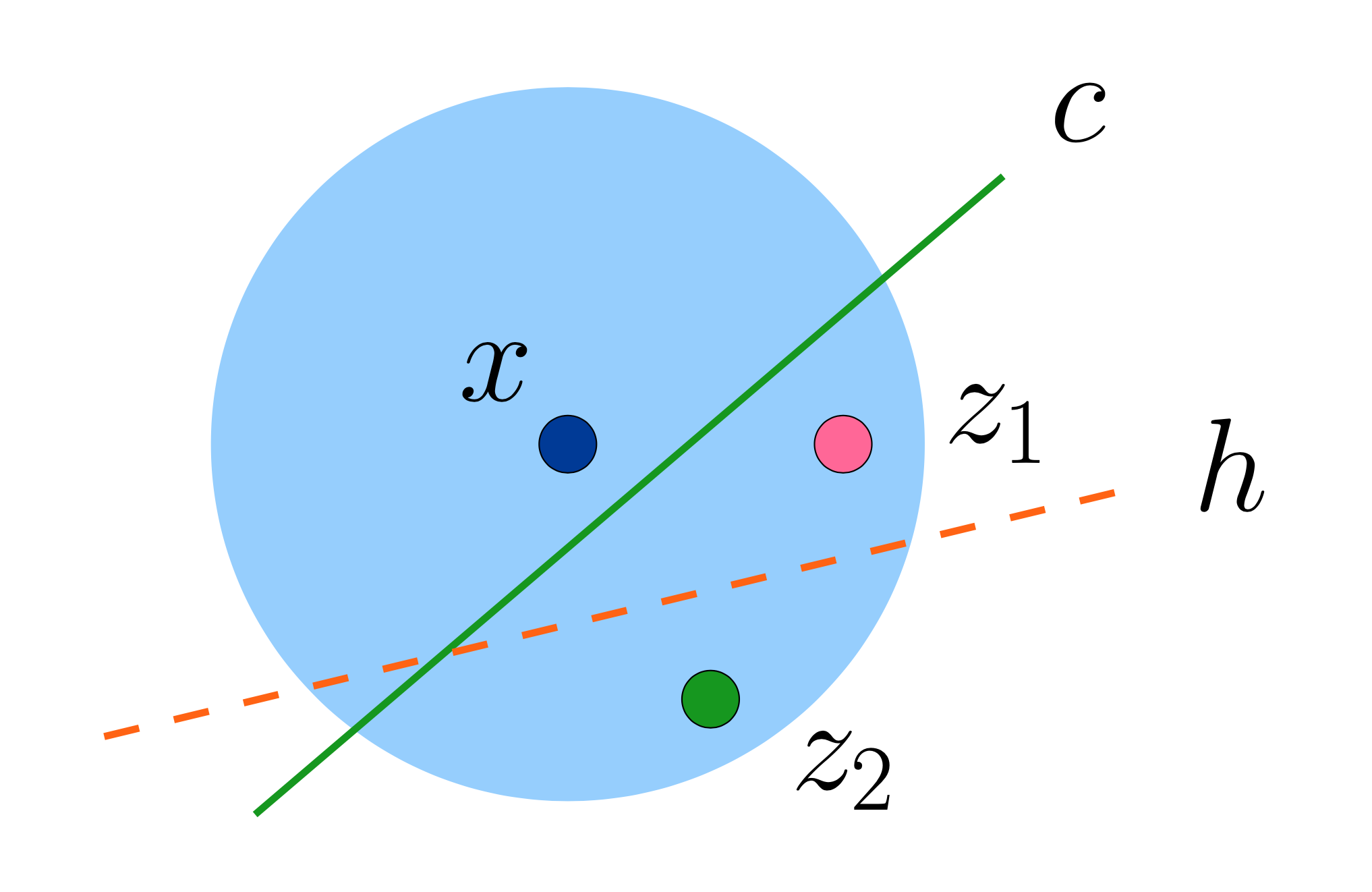
Figure 5: The natural point $x$ has robust loss of 1 with respect to both notions of robustness: $z_{1}$ is a counterexample for exact-in-the-ball robustness (as $c(z_{1})\neq h(z_{1})$), and $z_{2}$ for constant-in-the-ball robustness (as $c(x)\neq h(z_{2})$).

An obvious advantage of the constant-in-the-ball risk over the exact-in-the-ball version is that, in the former, evaluating the loss at point $x\in\mathcal{X}$ requires only knowledge of the correct label of $x$ and the hypothesis $h$. In particular, this definition can also be carried over to the non-realizable setting, in which there is no target, but rather a joint distribution on $\mathcal{X}\times\mathcal{Y}$. Then Equation 8 becomes $\underset{{(x,y)\sim D}}{\Pr}\left(\exists z\in B_{\rho}(x):h(z)\neq y\right)$.

Despite the advantages of the constant-in-the-ball risk, from a foundational point of view this notion of risk has some drawbacks: under this definition, it is possible to have strictly positive, and even sometimes constant, robust risk in the case that $h=c$. In fact, this view of robustness can in some circumstances be in conflict with accuracy in the traditional sense as pointed out by (Tsipras et al., (2019)). More in line with our work, Chowdhury and Urner, (2022) argue for robustness to be considered as a locally adaptive measure, where sometimes a label change is justified.

Example 4.3.

Under the uniform distribution, for $c\in\textsf{MON-CONJ}$ of constant length $k$, $\mathsf{R}_{1}^{C}(c,c)\geq\underset{{x\sim D}}{\Pr}\left(\exists!i\in[n]\;.\;c(x)\neq c(x^{\oplus i})\right)=\frac{k+1}{2^{k}}$, and in the case of decision lists, any list $c$ of the form $((x_{i},0),(x_{j},1),\dots)$ satisfies $\mathsf{R}_{1}^{C}(c,c)\geq\underset{{x\sim D}}{\Pr}\left(x_{j}=1\right)=1/2$. In the case of parity functions, it suffices to flip one bit of the index set to switch the label, so under any distribution $\mathsf{R}^{C}_{\rho}(c,c)=1$ for any $\rho\geq 1$.

(a)

(b)

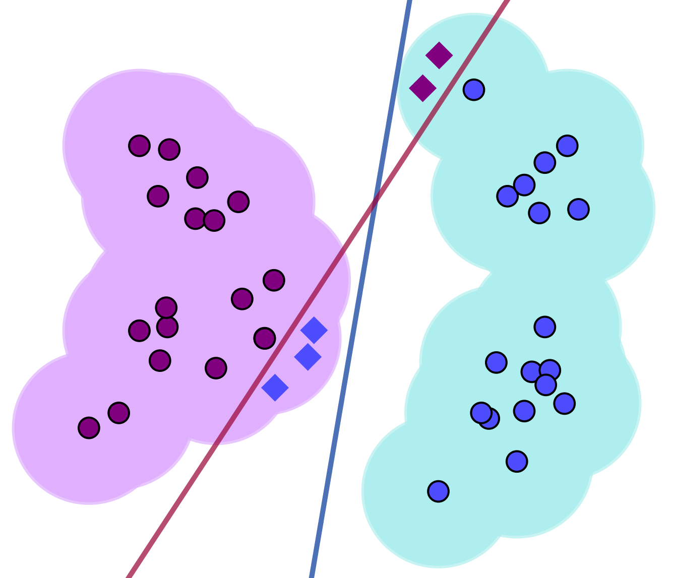
(c)

Figure 6: In all the examples above, the circles represent the support of the distribution, and the shaded region, its $\rho$-expansion (i.e., the points at a distance at most $\rho$ from points in the support of the distribution). (a) The support of the distribution is such that $\mathsf{R}^{C}_{\rho}(h,c)=0$ can only be achieved if $c$ is constant. (b) The $\rho$-expansion of the support of the distribution and target $c$ admit hypotheses $h$ such that $\mathsf{R}^{C}_{\rho}(h,c)=0$ (i.e., any $h$ that does not cross the shaded regions). (c) An example where $\mathsf{R}^{C}_{\rho}$ and $\mathsf{R}^{E}_{\rho}$ differ. The red concept, which crosses the shaded regions, is the target; the blue one is the hypothesis. The diamonds represent perturbed inputs which cause $\mathsf{R}^{E}_{\rho}(c,h)>0$, while $\mathsf{R}^{C}_{\rho}(h,c)=0$.

Let us note in passing that the risk functions $\mathsf{R}^{C}_{\rho}$ and $\mathsf{R}^{E}_{\rho}$ are in general incomparable. Figure 6(c) gives an example in which $\mathsf{R}^{C}_{\rho}=0$ and $\mathsf{R}^{E}_{\rho}>0$. Additionally, when we work in the hypercube, or a bounded input space, as $\rho$ becomes larger, we eventually require the function to be constant in the whole space. Essentially, to $\rho$-robustly learn in the constant-in-the-ball realizable setting, we require concept and distribution pairs to be represented as two sets $D_{+}$ and $D_{-}$ whose $\rho$-expansions don’t intersect, as illustrated in Figures 6(a) and 6(b).

We finish by pointing out that, in some cases in the (standard) realizable setting, the target $c$ is not the robust risk minimizer for $\rho=1$: the constant concept is! This is easy to see for parity functions, as $\mathsf{R}_{1}^{C}(c,0)=\mathsf{R}_{1}^{C}(c,1)=1/2$ under the uniform distribution while ${R}_{1}^{C}(c,c)=1$. A similar result holds for monotone conjunctions:

Proposition 4.4.

Under the uniform distribution, for any non-constant concept $c\in\textsf{MON-CONJ}$, we have that $\mathsf{R}_{1}^{C}(c,c)>\mathsf{R}_{1}^{C}(c,0)$.

Proof.

Let $\mathcal{X}=\left\{0,1\right\}^{n}$ and $D$ be the uniform distribution on $\mathcal{X}$. Let $c(x)=x_{1}\wedge\dots\wedge x_{k}$ for some $k\in[n]$. Then,

$$\mathsf{R}_{1}^{C}(c,c) =\underset{{x\sim D}}{\Pr}\left(\exists z\in B_{\rho}(x)\;.\;c(z)\neq c(x)\right)$$

$$=\underset{{x\sim D}}{\Pr}\left(c(x)=1\right)+\underset{{x\sim D}}{\Pr}\left(\exists!i\in[k]\;.\;x_{i}=0\right)$$

$$=\mathsf{R}_{1}^{C}(c,0)+\underset{{x\sim D}}{\Pr}\left(\exists!i\in[k]\;.\;x_{i}=0\right)$$

$$>\mathsf{R}_{1}^{C}(c,0)\enspace.$$

∎

Property	$\mathsf{R}^{C}_{\rho}$: constant-in-the-ball	$\mathsf{R}^{E}_{\rho}$: exact-in-the-ball
$\mathsf{R}_{\rho}(c,c)=0$?	✗	✓
$c=\arg\min_{h}\mathsf{R}_{\rho}(c,h)$?	✗	✓
$S$ enough to evaluate $\widehat{\mathsf{R}_{\rho}}$?	✓	✗
Behaviour of $h$ as $\rho\rightarrow n$	$h=$ constant	$h=c$ (exact)

Table 1: The pros and cons of the two robust risk functions. The last line refers to the behaviour of hypotheses minimizing the robust risk as the perturbation region increases. At the extreme case, when the perturbation region is the whole space, the robust risk minimizer for the constant-in-the-ball risk is a constant function, while it is the target for the exact-in-the-ball risk (as we require exact learning).

The discussion above, which pertains to the boolean hypercube, makes apparent the fact that the exact-in-the-ball and constant-in-the-ball definitions of robust risk both rely on different distributional and concept class assumptions. The constant-in-the-ball notion of robust risk relies on a strong distributional assumption (for e.g., a margin condition) and/or on the stability of functions in the concept class. The exact-in-the-ball is more relevant in cases where we cannot assume that the probability mass near the boundary is small, and wish to be correct with respect to the target function. Table 1 summarizes the advantages and disadvantages of both robust risks. Figure 7 shows real-life examples where such assumptions can come into play.

Figure 7: Images from the CIFAR-10 (above) and MNIST (below) datasets, respectively from (Krizhevsky and Hinton,, 2009) and (LeCun,, 1998). While the margin assumption generally holds for CIFAR (e.g., the “boat” and “dog” classes are well-separated), this is not necessarily the case for MNIST (the three above could easily be transformed into an eight, and the left-hand side picture could be a one or a seven).

Overall, choosing a robust risk function should depend on the learning problem at hand, and it is possible that other robustness frameworks could bring more nuance and faithfulness to practical robustness considerations. For the moment, to lay the foundations of robust learnability, we will work with the exact-in-the-ball notion of robustness in the PAC framework. Our choice of robust risk comes from the fact that the constant-in-ball risk is much better understood than for the exact-in-the-ball one (most papers we have mentioned in Chapter 2 have used the former).

Having settled on a risk function, we now formulate the definition of robust learning. For our purposes a concept class is a family $\mathcal{C}=\{\mathcal{C}_{n}\}_{n\in\mathbb{N}}$, with $\mathcal{C}_{n}$ a class of functions from $\{0,1\}^{n}$ to $\{0,1\}$. Likewise, a distribution class is a family $\mathcal{D}=\{\mathcal{D}_{n}\}_{n\in\mathbb{N}}$, with $\mathcal{D}_{n}$ a set of distributions on $\{0,1\}^{n}$. Finally, a robustness function is a function $\rho:\mathbb{N}\rightarrow\mathbb{N}$, which is fixed a priori.

Definition 4.5.

Fix a function $\rho:\mathbb{N}\rightarrow\mathbb{N}$. We say that an algorithm $\mathcal{A}$ efficiently $\rho$-robustly learns a concept class $\mathcal{C}$ with respect to distribution class $\mathcal{D}$ if there exists a polynomial $\text{poly}(\cdot,\cdot,\cdot,\cdot)$ such that for all $n\in\mathbb{N}$, all target concepts $c\in\mathcal{C}_{n}$, all distributions $D\in\mathcal{D}_{n}$, and all accuracy and confidence parameters $\epsilon,\delta>0$, if $m\geq\text{poly}(n,1/\epsilon,1/\delta,\text{size}(c))$, whenever $\mathcal{A}$ is given access to a sample $S\sim D^{m}$ labelled according to $c$, it outputs a polynomially evaluatable function $h:\{0,1\}^{n}\rightarrow\{0,1\}$ such that $\underset{{S\sim D^{m}}}{\Pr}\left(\mathsf{R}^{E}_{\rho(n)}(h,c)<\epsilon\right)>1-\delta$.

Note that our definition of robust learnability requires polynomial sample complexity and allows improper learning (the hypothesis $h$ need not belong to the concept class $\mathcal{C}_{n}$).

9.2 A Separation between PAC and Robust Learning

In the standard PAC framework, a hypothesis $h$ is considered to have zero risk with respect to a target concept $c$ when $\underset{{x\sim D}}{\Pr}\left(h(x)\neq c(x)\right)=0$. We have remarked that exact learnability (in the sense that $c=h$ on all of $\mathcal{X}$, not just the support of the distribution) implies robust learnability; next we give an example of a concept class $\mathcal{C}$ and distribution $D$ such that $\mathcal{C}$ is PAC learnable under $D$ with zero risk and yet cannot be robustly learned under $D$ (regardless of the sample complexity).

Lemma 4.6.

The class of dictators is not 1-robustly learnable (and thus not robustly learnable for any $\rho\geq 1$) with respect to the robust risk of Definition 4.1 in the distribution-free setting.

Proof.

Let $c_{1}$ and $c_{2}$ be the dictators on variables $x_{1}$ and $x_{2}$, respectively. Let $D$ be such that $\underset{{x\sim D}}{\Pr}\left(x_{1}=x_{2}\right)=1$ and $\underset{{x\sim D}}{\Pr}\left(x_{k}=1\right)=\frac{1}{2}$ for $k\geq 3$. Draw a sample $S\sim D^{m}$ and label it according to $c\sim U(c_{1},c_{2})$. By the choice of $D$, the elements of $S$ will have the same label regardless of whether $c_{1}$ or $c_{2}$ was picked. However, for $x\sim D$, it suffices to flip any of the first two bits to cause $c_{1}$ and $c_{2}$ to disagree on the perturbed input. We can easily show that, for any $h\in\left\{0,1\right\}^{\mathcal{X}}$, $\mathsf{R}^{E}_{1}(h,c_{1})+\mathsf{R}^{E}_{1}(h,c_{2})\geq\mathsf{R}^{E}_{1}(c_{1},c_{2})=1.$ Then

$$\underset{c\sim U(c_{1},c_{2})}{\mathbb{E}}\underset{{S\sim D^{m}}}{\mathbb{E}}\left[\mathsf{R}^{E}_{1}(h,c)\right]\geq 1/2\enspace.$$

We conclude that one of $c_{1}$ or $c_{2}$ has robust risk at least 1/2. ∎

Note that a PAC learning algorithm with error probability threshold $\varepsilon=1/3$ will either output $c_{1}$ or $c_{2}$ and will hence have standard risk zero.

The result above highlights an important distinction between standard and robust learning. We will further study this separation in the next section.

10 The Distribution-Free Assumption

In this section, we show that no non-trivial concept class is efficiently 1-robustly learnable in the boolean hypercube, implying that such a class is also not efficiently $\rho$-robustly learnable for any $\rho\geq 1$. As a consequence, there exists a fundamental separation between the standard PAC learning setting and its robust counterpart. Indeed, (efficient) robust learnability in the distribution-free setting would require access to a more powerful learning model or distributional assumptions when considering a learner who only has access to the random example oracle $\mathsf{EX}(c,D)$.

We start by defining trivial concept classes.

Definition 4.7.

Let $\mathcal{C}_{n}$ be a concept class on $\left\{0,1\right\}^{n}$, and define $\mathcal{C}=\bigcup_{n\geq 1}\mathcal{C}_{n}$. We say that a class of functions is trivial if $\mathcal{C}_{n}$ has at most two functions, which moreover differ on every point.

A simple example of a trivial concept class is the set of constant functions $\left\{0,1\right\}$. More generally, once a function in $\mathcal{C}$ is fixed, there is only one (uniquely defined) function that can be added to $\mathcal{C}$ and preserve its triviality. We show below that these are the only classes that are distribution-free robustly learnable.

Theorem 4.8.

For any concept class $\mathcal{C}$, $\mathcal{C}$ is efficiently distribution-free robustly learnable iff it is trivial.

Note that this is in stark contrast with the work of Montasser et al., (2019), which gives distribution-free robust learning guarantees for the constant-in-the-ball notion of robustness. This approach relies on an improper learner and a sample inflation made possible by the realizability of the learning problem under the constant-in-the-ball robust risk. The agnostic case follows from a non-trivial reduction from the agnostic to the realizable setting. This highlights a fundamental difference between the constant-in-the-ball and exact-in-the-ball robustness guarantees. Indeed, to perform such a sample inflation technique in our setting, one would need to have knowledge outside the training sample; this is addressed in Chapter 6.

The idea behind the proof of Theorem 4.8 is a generalization of the proof of Lemma 4.6 that dictators are not robustly learnable. However, note that we construct a distribution whose support is all of $\mathcal{X}$. It is possible to find two hypotheses $c_{1}$ and $c_{2}$ and create a distribution such that $c_{1}$ and $c_{2}$ will with high probability look identical on samples of size polynomial in $n$ but have robust risk $\Omega(1)$ with respect to one another. Since any hypothesis $h$ in $\left\{0,1\right\}^{\mathcal{X}}$ will disagree either with $c_{1}$ or $c_{2}$ on a given point $x$ if $c_{1}(x)\neq c_{2}(x)$, by choosing the target hypothesis $c$ at random from $c_{1}$ and $c_{2}$, we can guarantee that $h$ won’t be robust against $c$ with positive probability. This shows that efficient robust learnability is in general impossible. However, the same argument as in Lemma 4.6 can be made to show that, even with infinite sample complexity, non-trivial classes are not robustly learnable. Finally, note that an analogous argument can be made for a more general setting (e.g., for the input space $\mathbb{R}^{n}$).

The proof of Theorem 4.8 relies on the following lemma, which states that the robust risk satisfies the triangle inequality:

Lemma 4.9.

Let $c_{1},c_{2}\in\{0,1\}^{\mathcal{X}}$ and fix a distribution on $\mathcal{X}$. Then for all $h:\left\{0,1\right\}^{n}\rightarrow\left\{0,1\right\}$

$$\mathsf{R}^{E}_{\rho}(c_{1},c_{2})\leq\mathsf{R}^{E}_{\rho}(h,c_{1})+\mathsf{R}^{E}_{\rho}(h,c_{2})\enspace.$$

Proof.

Let $x\in\left\{0,1\right\}^{n}$ be arbitrary, and suppose that $c_{1}$ and $c_{2}$ differ on some $z\in B_{\rho}(x)$. Then either $h(z)\neq c_{1}(z)$ or $h(z)\neq c_{2}(z)$. The result follows. ∎

We are now ready to prove Theorem 4.8.

Proof of Theorem 4.8.

First, if $\mathcal{C}$ is trivial, we need at most one example to identify the target function.

For the other direction, suppose that $\mathcal{C}$ is non-trivial, and for a given $c\in\mathcal{C}$, denote by $I_{c}\subseteq[n]$ the index set of relevant variables in the function $c$. We first start by fixing any learning algorithm and polynomial sample complexity function $m$. Let $\eta=\frac{1}{2^{\omega(\log n)}}$, $0<\delta<\frac{1}{2}$, and note that for any constant $a>0$,

$$\underset{n\rightarrow\infty}{\lim}\;n^{a}\log(1-\eta)^{-1}=0\enspace,$$

and so any polynomial in $n$ is $o\left(\left(\log(1/(1-\eta))\right)^{-1}\right)$. Then it is possible to choose $n_{0}$ such that for all $n\geq n_{0}$,

$$m\leq\frac{\log(1/\delta)}{2n\log(1-\eta)^{-1}}\enspace.$$ (9)

Since $\mathcal{C}$ is non-trivial, we can choose concepts $c_{1},c_{2}\in\mathcal{C}_{n}$ and points $x,x^{\prime}\in\left\{0,1\right\}^{n}$ such that $c_{1}$ and $c_{2}$ agree on $x$ but disagree on $x^{\prime}$. This implies that there exists a point $z\in\left\{0,1\right\}^{n}$ such that (i) $c_{1}(z)=c_{2}(z)$ and (ii) it suffices to change only one bit in $I:=I_{c_{1}}\cup I_{c_{2}}$ to cause $c_{1}$ to disagree on $z$ and its perturbation. Let $D$ be a product distribution such that

$$\underset{{x\sim D}}{\Pr}\left(x_{i}=z_{i}\right)=\begin{cases}1-\eta&\quad\text{if }i\in I\\ \frac{1}{2}&\quad\text{otherwise}\end{cases}\enspace.$$

Draw a sample $S\sim D^{m}$ and label it according to $c\sim U(c_{1},c_{2})$. Then,

$$\underset{{S\sim D^{m}}}{\Pr}\left(\forall x\in S\quad c_{1}(x)=c_{2}(x)\right)\geq\left(1-\eta\right)^{m|I|}\enspace.$$ (10)

Bounding the RHS below by $\delta>0$, we get that, as long as

$$m\leq\frac{\log(1/\delta)}{|I|\log(1-\eta)^{-1}}\enspace,$$

Equation 10 holds with probability at least $\delta$. This is enabled by the requirement from Equation 9.

However, if $x=z$, then it suffices to flip one bit of $x$ to get $x^{\prime}$ such that $c_{1}(x^{\prime})\neq c_{2}(x^{\prime})$. Then,

$$\mathsf{R}^{E}_{\rho}(c_{1},c_{2})\geq\underset{{x\sim D}}{\Pr}\left(x_{I}=z_{I}\right)=\left(1-\eta\right)^{|I|}\enspace.$$ (11)

The constraints on $\eta$ and the fact that $|I|\leq n$ are sufficient to guarantee that the RHS is $\Omega(1)$. Let $\alpha>0$ be a constant such that $\mathsf{R}^{E}_{\rho}(c_{1},c_{2})\geq\alpha$.

We can use the same reasoning as in Lemma 4.9 to argue that, for any $h\in\left\{0,1\right\}^{\mathcal{X}}$,

$$\mathsf{R}^{E}_{1}(c_{1},h)+\mathsf{R}^{E}_{1}(c_{2},h)\geq\mathsf{R}^{E}_{1}(c_{1},c_{2})\enspace.$$

Finally, we can show that

$$\underset{c\sim U(c_{1},c_{2})}{\mathbb{E}}\underset{{S\sim D^{m}}}{\mathbb{E}}\left[\mathsf{R}^{R}_{1}(h,c)\right]\geq\alpha\delta/2,$$

hence there exists a target $c$ with expected robust risk bounded below by a constant.∎

In the next section, we will show that, even when looking at problems with distributional assumptions, robust learning can be hard from an information-theoretic point of view.

11 An Adversarial Sample Complexity Lower Bound

In this section, we will show that any robust learning algorithm for monotone conjunctions under the uniform distribution must have an exponential sample-complexity dependence on the adversary’s budget $\rho$. This result extends to any superclass of monotone conjunctions, such as CNF formulas, decision lists and linear classifiers. It is a generalization of Theorem 13 in Gourdeau et al., (2021), an earlier version of the work presented in this thesis, which shows that no sample-efficient robust learning algorithm exists for monotone conjunctions against adversaries that can perturb $\omega(\log(n))$ bits of the input under the uniform distribution.

Monotone conjunctions are perhaps the simplest class of functions to study in learning theory. Recall that a conjunction $c$ over $\{0,1\}^{n}$ can be represented by a set of literals $l_{1},\dots,l_{k}$, where, for $x\in\mathcal{X}_{n}$, $c(x)=\bigwedge_{i=1}^{k}l_{i}$. Monotone conjunctions are the subclass of conjunctions where negations are not allowed, i.e. all literals are of the form $l_{i}=x_{j}$ for some $j\in[n]$. The standard PAC learning algorithm to learn conjunctions is outlined in Algorithm 1 in Section 6.3, and can straightforwardly be adapted for monotone conjunctions, with the slight distinction that the initial hypothesis is $\bigwedge_{i\in[n]}x_{i}$.

Theorem 4.10.

Fix a positive increasing robustness function $\rho:\mathbb{N}\rightarrow\mathbb{N}$. If $\rho$ is a function of the input dimension $n$, then for $\kappa<2$ and sufficiently large $n$, any $\rho(n)$-robust learning algorithm for MON-CONJ has a sample complexity lower bound of $2^{\kappa\rho(n)}$ under the uniform distribution. Otherwise, the same lower bound holds whenever $\rho$ is a sufficient large constant (with respect to $\kappa$).

The idea behind the proof is to show that, for any $\kappa<2$, there exists a sufficiently large input dimension (that depends on $\kappa$ and the function $\rho$) such that a sample of size $2^{\kappa\rho}$ from the uniform distribution will not be able to distinguish between two disjoint conjunctions of length $2\rho$. However, the robust risk between these two conjunctions can be lower bounded by a constant. Hence, there does not exist a robust learning algorithm with sample complexity $2^{\kappa\rho}$ that works for the uniform distribution, and arbitrary input dimension and confidence and accuracy parameters.

Recall that the sample complexity of PAC learning conjunctions is $\Theta(n)$ in the non-adversarial setting. On the other hand, our adversarial lower bound in terms of the robust parameter is superlinear in $n$ as soon as the adversary can perturb more than $\log(\sqrt{n})$ bits of the input.

The proof of Theorem 4.10 relies on the lemmas below, as well as Lemma 4.9. Lemma 4.11 lower bounds the robust risk between two disjoint monotone conjunctions as a function of the adversarial budget $\rho$, while Lemma 4.12 lower bounds the probability that these two concepts are indistinguishable on a polynomially-sized sample.

Lemma 4.11.

Under the uniform distribution, for any $n\in\mathbb{N}$, disjoint $c_{1},c_{2}\in{\textsf{MON-CONJ}}$ of even length $3\leq l\leq n/2$ on $\left\{0,1\right\}^{n}$ and robustness parameter $\rho=l/2$, we have that $\mathsf{R}_{\rho}(c_{1},c_{2})$ is bounded below by a constant that can be made arbitrarily close to $\frac{1}{2}$ as $l$ (and thus $\rho$) increases.

Proof.

For a hypothesis $c\in{\textsf{MON-CONJ}}$, let $I_{c}$ be the set of variables in $c$. Let $c_{1},c_{2}\in\mathcal{C}$ be as in the statement of the lemma. Then the robust risk $\mathsf{R}_{\rho}(c_{1},c_{2})$ is bounded below by

$$\underset{{x\sim D}}{\Pr}\left(c_{1}(x)=0\wedge x\text{ has at least $\rho$ 1's in }I_{c_{2}}\right)\geq(1-2^{-2\rho})/2\enspace.$$

∎

Now, the following lemma shows that, for sufficiently large input dimensions, a sample of size $2^{\kappa\rho}$ from the uniform distribution will look constant with probability $1/2$ if labelled by two disjoint monotone conjunctions of length $2\rho$.

Lemma 4.12.

For any constant $\kappa<2$, for any robustness parameter $\rho\leq n/4$, for any disjoint monotone conjunctions $c_{1},c_{2}$ of length $2\rho$, there exists $n_{0}$ such that for all $n\geq n_{0}$, a sample $S$ of size $2^{\kappa\rho}$ sampled i.i.d. from $D$ will have that $c_{1}(x)=c_{2}(x)=0$ for all $x\in S$ with probability at least $1/2$.

Proof.

We begin by bounding the probability that $c_{1}$ and $c_{2}$ agree on an i.i.d. sample of size $m$. We have

$$\underset{{S\sim D^{m}}}{\Pr}\left(\forall x\in S\cdot c_{1}(x)=c_{2}(x)=0\right)=\left(1-\frac{1}{2^{2\rho}}\right)^{2m}\enspace.$$ (12)

In particular, if

$$m\leq\frac{\log(2)}{2\log(2^{2\rho}/(2^{2\rho}-1))}\enspace,$$ (13)

then the RHS of Equation 12 is at least $1/2$.

Now, let us consider the following limit, where $\rho$ is a function of the input parameter $n$:

$$\underset{n\rightarrow\infty}{\lim}\;2^{\kappa\rho}\log\left(\frac{2^{2\rho}}{2^{2\rho}-1}\right) =\frac{-\log(4)}{\kappa\log(2)}\;\underset{n\rightarrow\infty}{\lim}\;\frac{2^{\kappa\rho}}{1-2^{2\rho}}$$

$$=\frac{-\log(4)}{\kappa\log(2)}\;\frac{\kappa\log(2)}{-2\log(2)}\underset{n\rightarrow\infty}{\lim}\;\frac{2^{\kappa\rho}}{2^{2\rho}}$$

$$=\underset{n\rightarrow\infty}{\lim}\;2^{(\kappa-2)\rho}$$

$$=\begin{cases}0&\text{if $\kappa<2$}\\ 1&\text{if $\kappa=2$}\\ \infty&\text{if $\kappa>2$}\end{cases}\enspace,$$

where the first two equalities follow from l’Hôpital’s rule.

Thus if $\kappa<2$ then $2^{\kappa\rho}$ is $o\left(\left(\log\left(\frac{2^{2\rho}}{2^{2\rho}-1}\right)\right)^{-1}\right)$.

∎

Remark 4.13.

Note that for a given $\kappa<2$, the lower bound $2^{\kappa\rho}$ holds only for sufficiently large $\rho(n)$. By looking at Equation 12, and letting $m=2^{\rho}$, we get that $\rho(n)\geq 2$ is a sufficient condition for it to hold. If we want a lower bound for robust learning that is larger than that of standard learning (where the dependence is $\Theta(n)$) for a $\log(n)$ adversary, setting $m=2^{1.7\rho}$ and requiring $\rho(n)\geq 6$, for e.g., would be sufficient.

We are now ready to prove Theorem 4.10.

Proof of Theorem 4.10.

Fix any algorithm $\mathcal{A}$ for learning MON-CONJ. We will show that the expected robust risk between a randomly chosen target function and any hypothesis returned by $\mathcal{A}$ is bounded below by a constant.

Let $\delta=1/2$, and fix a positive increasing adversarial-budget function $\rho(n)\leq n/4$ ($n$ is not yet fixed). Let $m(n)=2^{\kappa\rho(n)}$ for an arbitrary $\kappa<0$. Let $n_{0}$ be as in Lemma 4.12, where $m(n)$ is the fixed sample complexity function. Then Equation (13) in the proof of Lemma 4.12 holds for all $n\geq n_{0}$.

Now, let $D$ be the uniform distribution on $\left\{0,1\right\}^{n}$ for $n\geq\max(n_{0},3)$, and choose $c_{1}$, $c_{2}$ as in Lemma 4.11. Note that $\mathsf{R}_{\rho}(c_{1},c_{2})>\frac{5}{12}$ by the choice of $n$. Pick the target function $c$ uniformly at random between $c_{1}$ and $c_{2}$, and label $S\sim D^{m(n)}$ with $c$. By Lemma 4.12, $c_{1}$ and $c_{2}$ agree with the labeling of $S$ (which implies that all the points have label $0$) with probability at least $\frac{1}{2}$ over the choice of $S$.

Define the following three events for $S\sim D^{m}$:

$$\mathcal{E}:\;{c_{1}}_{|S}={c_{2}}_{|S}\;,\enspace\mathcal{E}_{c_{1}}:\;c=c_{1}\;,\enspace\mathcal{E}_{c_{2}}:\;c=c_{2}\enspace.$$

Then,

$$\underset{{c,S}}{\mathbb{E}}\left[\mathsf{R}_{\rho}(\mathcal{A}(S),c)\right] \geq\underset{{c,S}}{\Pr}\left(\mathcal{E}\right)\underset{{c,S}}{\mathbb{E}}\left[\mathsf{R}_{\rho}(\mathcal{A}(S),c)\;|\;\mathcal{E}\right]$$

$$>\frac{1}{2}(\underset{{c,S}}{\Pr}\left(\mathcal{E}_{c_{1}}\right)\underset{{S}}{\mathbb{E}}\left[\mathsf{R}_{\rho}(\mathcal{A}(S),c)\;|\;\mathcal{E}\cap\mathcal{E}_{c_{1}}\right]+\underset{{c,S}}{\Pr}\left(\mathcal{E}_{c_{2}}\right)\underset{{S}}{\mathbb{E}}\left[\mathsf{R}_{\rho}(\mathcal{A}(S),c)\;|\;\mathcal{E}\cap\mathcal{E}_{c_{2}}\right])$$

$$=\frac{1}{4}\;\underset{{S}}{\mathbb{E}}\left[\mathsf{R}_{\rho}(\mathcal{A}(S),c_{1})+\mathsf{R}_{\rho}(\mathcal{A}(S),c_{2})\;|\;\mathcal{E}\right]$$

$$\geq\frac{1}{4}\;\underset{{S}}{\mathbb{E}}\left[\mathsf{R}_{\rho}(c_{2},c_{1})\right]$$

$$=\frac{5}{48}\enspace,$$

where the first inequality is due to the Law of Total Expectation. The strict inequality comes from Lemma 4.12, the last inequality from Lemma 4.9, and the last equality from Lemma 4.11. ∎

Comparison with Diochnos et al., (2018, 2020)

First, Diochnos et al., (2018) considers the robustness of monotone conjunctions under the uniform distribution on the boolean hypercube for the exact-in-the-ball notion of risk. However, Diochnos et al., (2018) does not address the sample and computational complexity of learning: their results rather concern the ability of an adversary to magnify the missclassification error of any hypothesis with respect to any target function by perturbing the input. For example, they show that an adversary who can perturb $\Theta(\sqrt{n})$ bits can increase the missclassification probability from $0.01$ to $1/2$. The main tool used in Diochnos et al., (2018) is the isoperimetric inequality for the boolean hypercube, which gives lower bounds on the volume of the expansions of arbitrary subsets. On the other hand, we use the probabilistic method to establish the existence of a single hard-to-robustly-learn target concept for any given algorithm with sample complexity exponential in $\rho$.

The work of Diochnos et al., (2020) shows an exponential lower bound on the sample complexity of robust PAC learning of a wide family of concept classes, which are called $\alpha$-close, meaning that there must exist two concepts in the class that have (standard) error $\alpha$. These bounds hold under Normal Lévy distributions (which include product distributions under the Hamming distance in $\left\{0,1\right\}^{n}$) against all adversaries that can perturb up to $o(n)$ bits. Closer to our results of this section, they also show a superpolynomial lower bound in sample complexity against adversaries that can perturb $\widetilde{\Theta}(\sqrt{n})$ bits. This thesis obtains the same result against a weaker adversary in the special case of the uniform distribution: we show that a weaker adversary, who can perturb only $\omega(\log n)$ bits, renders it impossible to robustly learn monotone conjunctions (and any superclass) with polynomial sample complexity. In fact, we will show in Section 12 that $\Theta(\log n)$ is indeed the threshold for the efficient robust PAC learning of this class under log-Lipschitz distributions, which include the uniform distribution.

12 Robust Learnability Against a Logarithmically-Bounded Adversary

In the previous section, we exhibited an exponential dependence on the adversary’s budget to robustly learn monotone conjunctions under the uniform distribution. We now turn our attention to a wider family of distributions, log-Lipschitz distributions, and show that robust learnability can be guaranteed in this setting whenever the adversary is logarithmically bounded. These results show that the sample complexity of robust learning in our setting is controlled by the adversary’s budget.

12.1 Log-Lipschitz Distributions

A thorough introduction to log-Lipschitz distributions can be found in Section 7, but we will recall the formal definition here.

Definition 3.22. A distribution $D$ on $\left\{0,1\right\}^{n}$ is said to be $\alpha$-$\log$-Lipschitz if for all input points $x,x^{\prime}\in\left\{0,1\right\}^{n}$, if $d_{H}(x,x^{\prime})=1$, then $|\log(D(x))-\log(D(x^{\prime}))|\leq\log(\alpha)$.

While it may be tempting to work under product distributions over the instance space $\left\{0,1\right\}^{n}$, as many concentration bounds and Fourier analysis tools are readily available for this setting, independence between features is usually not a reasonable assumption to make in practice. Indeed, it often happens that some features are correlated, e.g., a person’s height and weight. By loosening the product distribution requirement to a log-Lipschitz one, we allow for some dependence between the features. However, from a robustness point of view, it is sensible to ensure that features are not too dependent on each other (which is also encapsulated by log-Lipschitzness). Taking this to the extreme, suppose a feature has been duplicated, i.e., there exist indices $i,j$ in $[n]$ such that $x_{i}=x_{j}$ for all points in the support of the distribution. Then, an instance such that $x_{i}=\bar{x_{j}}$ does not represent a meaningful instance of the problem to be learned, and perhaps it would be unfair to require an algorithm to perform well in such cases. Moreover, it is unclear how one would measure robustness performance in this scenario.

In a sense, log-Lipschitz distributions encapsulate a natural desideratum when considering both robustness guarantees and realistic assumptions on the data, and furthermore provide a sound abstract framework to study robust learnability.

12.2 A Robustness Guarantee

We now look at robustly learning monotone conjunctions on $\left\{0,1\right\}^{n}$ under log-Lipschitz distributions when the adversary can flip $\log(n)$ bits of the input at test time. We remark that, when one has access to membership queries, one can easily exactly learn monotone conjunctions over the whole input space: we start with the instance where all bits are 1 (which is always a positive example, as the constant function 0 does not belong to this class), and we can test whether each variable is in the target conjunction by setting the corresponding bit to 0 and requesting the label. However, robustly learning monotone conjunctions with access to random examples only is not so straightforward, as positive examples, which are more informative than negative ones, could be difficult to come by under the underlying distribution.

We now formally state the main result of this section.

Theorem 4.14.

Let $\mathcal{D}=\{\mathcal{D}_{n}\}_{n\in\mathbb{N}}$, where $\mathcal{D}_{n}$ is a set of $\alpha$-$\log$-Lipschitz distributions on $\{0,1\}^{n}$ for all $n\in\mathbb{N}$. Then the class of monotone conjunctions is $\rho$-robustly learnable with respect to $\mathcal{D}$ for robustness function $\rho(n)=O(\log n)$.

This theorem combined with Theorem 4.10 shows that $\rho(n)=\log(n)$ is essentially the threshold for the efficient robust learnability of the class MON-CONJ. Note that here, and in all future results, we consider the constant $\alpha$ that parametrises the log-Lipschitz distribution to be fixed, and it appears explicitly in the sample complexity.

The main idea to prove Theorem 4.14 is that, on the one hand, it is possible to efficiently exactly learn the target conjunction if its length is logarithmic in the input dimension. On the other hand, we can otherwise efficiently $\rho$-robustly learn (but not necessarily exactly learn) longer conjunctions as the robustness parameter is logarithmic in the input dimension, and thus the adversary’s budget is insufficiently large to cause a label change (with high probability). This is a simple example that shows that robust learning does not necessarily imply exact learning.

Proof of Theorem 4.14.

We show that the algorithm $\mathcal{A}$ for PAC-learning monotone conjunctions (see Algorithm 1 in Chapter 3) is a robust learner for an appropriate choice of sample size. We start with the hypothesis $h(x)=\bigwedge_{i\in I_{h}}x_{i}$, where $I_{h}=[n]$. For each example $x$ in $S$, we remove $i$ from $I_{h}$ if $c(x)=1$ and $x_{i}=0$.

Let $\mathcal{D}$ be a class of $\alpha$-$\log$-Lipschitz distributions. Let $n\in\mathbb{N}$ and $D\in\mathcal{D}_{n}$. Suppose moreover that the target concept $c$ is a conjunction of $l$ variables. Fix $\varepsilon,\delta>0$. Let $\eta=\frac{1}{1+\alpha}$, and note that by Lemma 3.23, for any $S\subseteq[n]$ and $b_{S}\in\{0,1\}^{S}$, we have that $\eta^{|S|}\leq\underset{{x\sim D}}{\Pr}\left(x_{i}=b\right)\leq(1-\eta)^{|S|}$.

Claim 1.

If $m\geq\left\lceil\frac{\log n-\log\delta}{\eta^{l+1}}\right\rceil$ then given a sample $S\sim D^{m}$, algorithm $\mathcal{A}$ outputs $c$ with probability at least $1-\delta$.

Proof of Claim 1. Fix $i\in\{1,\ldots,n\}$. Algorithm $\mathcal{A}$ eliminates $i$ from the output hypothesis just in case there exists $x\in S$ with $x_{i}=0$ and $c(x)=1$. Now we have $\underset{{x\sim D}}{\Pr}\left(x_{i}=0\wedge c(x)=1\right)\geq\eta^{l+1}$ and hence

$$\underset{{S\sim D}}{\Pr}\left(\forall x\in S\cdot i\text{ remains in }I_{h}\right)\leq(1-\eta^{l+1})^{m}\leq e^{-m\eta^{l+1}}=\frac{\delta}{n}\,.$$

The claim now follows from union bound over $i\in\{1,\ldots,n\}$.

Claim 2.

If $l\geq\frac{8}{\eta^{2}}\log(\frac{1}{\varepsilon})$ and $\rho\leq\frac{\eta l}{2}$ then $\underset{{x\sim D}}{\Pr}\left(\exists z\in B_{\rho}(x)\cdot c(z)=1\right)\leq\varepsilon$.

Proof of Claim 2. Define a random variable $Y=\sum_{i\in I_{c}}\mathbb{I}(x_{i}=1)$. We simulate $Y$ by the following process. Let $X_{1},\dots,X_{l}$ be random variables taking value in $\{0,1\}$, and which may be dependent. Let $D_{i}$ be the marginal distribution on $X_{i}$ conditioned on $X_{1},\dots,X_{i-1}$. This distribution is also $\alpha$-$\log$-Lipschitz by Lemma 3.23, and hence,

$$\underset{{X_{i}\sim D_{i}}}{\Pr}\left(X_{i}=1\right)\leq 1-\eta\enspace.$$ (14)

Since we are interested in the random variable $Y$ representing the number of 1’s in $X_{1},\dots,X_{l}$, we define the random variables $Z_{1},\dots,Z_{l}$ as follows:

$$Z_{k}=\left(\sum_{i=1}^{k}X_{i}\right)-k(1-\eta)\enspace,$$

with the convention that $Z_{0}=0$. The sequence $Z_{0},Z_{1},\dots,Z_{l}$ is a supermartingale with respect to $X_{1},\dots,X_{l}$:

$$\underset{{}}{\mathbb{E}}\left[Z_{k+1}\;|\;X_{1},\dots,X_{k}\right] =\underset{{}}{\mathbb{E}}\left[Z_{k}+X_{k+1}^{\prime}-(1-\eta)\;|\;X^{\prime}_{1},\dots,X^{\prime}_{k}\right]$$

$$=Z_{k}+\underset{{}}{\Pr}\left(X_{k+1}^{\prime}=1\;|\;X^{\prime}_{1},\dots,X^{\prime}_{k}\right)-(1-\eta)$$

$$\leq Z_{k}\enspace.$$ (by (31))

Now, note that all $Z_{k}$’s satisfy $|Z_{k+1}-Z_{k}|\leq 1$, and that $Z_{l}=Y-l(1-\eta)$. We can thus apply the Azuma-Hoeffding (A.H.) inequality (see Section 7 for details) to get

$$\underset{{}}{\Pr}\left(Y\geq l-\rho\right) \leq\underset{{}}{\Pr}\left(Y\geq l(1-\eta)+\sqrt{2\ln(1/\varepsilon)l}\right)$$

$$=\underset{{}}{\Pr}\left(Z_{l}-Z_{0}\geq\sqrt{2\ln(1/\varepsilon)l}\right)$$

$$\leq\exp\left(-\frac{\sqrt{2\ln(1/\varepsilon)l}^{2}}{2l}\right)$$ (A.H.)

$$=\varepsilon\enspace,$$

where the first inequality holds from the given bounds on $l$ and $\rho$:

$$l-\rho =(1-\eta)l+\frac{\eta l}{2}+\frac{\eta l}{2}-\rho$$

$$\geq(1-\eta)l+\frac{\eta l}{2} \rho\leq\frac{\eta l}{2}$$ (since )

$$\geq(1-\eta)l+\sqrt{2\log(1/\varepsilon)l}\enspace. l\geq\frac{8}{\eta^{2}}\log(\frac{1}{\varepsilon})$$ (since )

This completes the proof of Claim 2.

We now combine Claims 1 and 2 to prove the theorem. Define $l_{0}:=\max(\frac{2}{\eta}\log n,\frac{8}{\eta^{2}}\log(\frac{1}{\varepsilon}))$. Define $m:=\left\lceil\frac{\log n-\log\delta}{\eta^{l_{0}+1}}\right\rceil$. Note that $m$ is polynomial in $n$, $\delta$, $\varepsilon$.

Let $h$ denote the output of algorithm $\mathcal{A}$ given a sample $S\sim D^{m}$. We consider two cases. If $l\leq l_{0}$ then, by Claim 1, $h=c$ (and hence the robust risk is $0$) with probability at least $1-\delta$. If $l_{0}\leq l$ then, since $\rho=\log n$, we have $l\geq\frac{8}{\eta^{2}}\log(\frac{1}{\varepsilon})$ and $\rho\leq\frac{\eta l}{2}$ and so we can apply Claim 2. By Claim 2 we have

$$\mathsf{R}^{E}_{\rho}(h,c)\leq\underset{{x\sim D}}{\Pr}\left(\exists z\in B_{\rho}(x)\cdot c(z)=1\right)\leq\varepsilon$$

∎

Now that we have shown robust learnability against logarithmically-bounded adversaries, we define robustness thresholds, a term that will be used throughout this thesis.

Definition 4.15 (Robustness Threshold).

A robustness threshold for concept class $\mathcal{C}$ and distribution family $\mathcal{D}$ is an adversarial budget function $\rho:\mathbb{N}\rightarrow\mathbb{R}$ of the input dimension $n$ such that, if the adversary is allowed perturbations of magnitude $\rho(n)$, then there exists a sample-efficient $\rho(n)$-robust learning algorithm for $\mathcal{C}$ under $\mathcal{D}$, and if the adversary’s budget is $\omega(\rho(n))$, then such an algorithm does not exist.

As a consequence of Theorems 4.10 and 4.14, we get the following result.

Theorem 4.16.

The robustness threshold for MON-CONJ under log-Lipschitz distributions is $\rho(n)=\log(n)$.

As we will discuss further in the next chapter, we finish by remarking that the method employed to show efficient robust learnability in this section is to use a (proper) PAC-learning algorithm as a black box and control the accuracy parameter to ensure robustness to evasion attacks.

13 Summary

This chapter offered a thorough discussion on the choice of robust risk for evasion attacks. Settling on the exact-in-the-ball robust risk, we then showed that the standard PAC and robust learning settings are fundamentally different in that, contrary to the former, the latter requires distributional assumptions to ensure (efficient) learnability. But even when considering the natural uniform distribution, we showed that the efficient robust learning of monotone conjunctions, a very simple concept class, cannot be guaranteed against an adversary that has a superlogarithmic perturbation budget. However, we showed that this result is tight: guarantees can be obtained for logarithmically-bounded adversaries under log-Lipschitz distributions. Overall, these results show that the adversarial budget is a fundamental quantity in determining the sample complexity of robust learning under these distributional assumptions. This motivates the term robustness threshold, adversarial budget functions characterizing efficient robust learnability for a given distribution family. The next chapter will study the robustness thresholds of various concept classes under smoothness assumptions.

Chapter 5 Robustness Thresholds with Random Examples

In this chapter, we further explore the robustness thresholds (Definition 4.15) of various concept classes under distributional assumptions, again with respect to the exact-in-the-ball notion of robustness. In Section 14, we start by showing that exact (and thus robust) learning is possible for parities under log-Lipschitz distributions and majority functions under the uniform distribution. We then turn our attention to decision lists, where we show a robustness threshold of $\log n$ under log-Lipschitz distributions in Section 15. Section 16 concludes the technical contributions of this chapter by relating the standard and robust errors of decision trees.

In Section 15, we demonstrate the robust learnability of $k$-decision lists by first looking at the case where $k=1$, which forms the foundation of the generalization to $k$-$\mathsf{DL}$. This simpler case provides a substantial intuition behind the reasoning for the more complex case of $k>1$, while also giving better sample complexity bounds in the specific case $k=1$. We then distinguish two set-ups for the case $k>1$: (i) $2$-$\mathsf{DL}$ and monotone $k$-$\mathsf{DL}$, and (ii) non-monotone $k$-$\mathsf{DL}$. While the second case is more general, the first one results in better sample complexity upper bounds. Indeed, the dependence on $k$, which we consider to be a fixed constant, in the degree of the former is $\text{poly}(k)$, while it is $2^{\text{poly}(k)}$ for the latter.

This chapter concludes with Section 17, which summarizes the results of this chapter. As explained in more detail in that section, the methods in this chapter can be viewed as relating the mass of the error region between the target and hypothesis and the $\rho$-expansion of the error region, where $\rho$ is the adversarial budget. Indeed, the general, unifying approach in proving robustness thresholds in this work is to express the discrepancy between two functions (i.e., instances where they disagree) as a logical formula $\varphi$. We then relate the size of the set of satisfying assignments of $\varphi$ to the size of its expansion. This means that we can control the robust risk by controlling the standard risk, thus allowing the use of standard PAC-learning algorithms as black boxes for robust learning, provided the adversary is logarithmically-bounded.

14 Exact Learning

In the previous chapter, monotone conjunctions of sufficiently large length satisfied a certain form of stability, ensuring that one could obtain robust learning guarantees without the need to exactly learn them. In this section, we turn our attention to unstable concept classes, where one in general cannot ensure robustness without having learned the target exactly.

14.1 Parity Functions

In this section, we show that the concept class $\mathsf{PARITIES}$ of parity functions are efficiently exactly learnable under log-Lipschitz distributions. As these distributions have support on the whole input space, it follows that this implies efficient robust learning of parities.

Recall that parity functions are of the form $f_{I}(x)=\sum_{i\in I}x_{i}\bmod 2$, where $I\subseteq[n]$. Note that exact learning is necessary under our notion of robustness: if $I$ is non-empty, then every instance is on the decision boundary, as it suffices to flip a single bit in $I$ to cause $f_{I}$ to change label. The idea to show robust learnability of parity functions is to show that, for a class of $\alpha$-log-Lipschitz distributions, a proper PAC-learning algorithm can be used as a black box for exact learning.

Theorem 5.1.

$\mathsf{PARITIES}$ is exactly learnable under $\alpha$-log-Lipschitz distributions.

Proof.

Consider a proper PAC-learning algorithm $\mathcal{A}$ with sample complexity $\text{poly}(\cdot)$ for $\mathsf{PARITIES}$ (see e.g., Goldberg, (2006)). Let $\mathcal{D}$ be a family of $\alpha$-$\log$-Lipschitz distributions and let $D\in\mathcal{D}$ be arbitrary. Let $\epsilon,\delta>0$ be the accuracy and confidence parameters, $n$ be the input dimension, and $c(x)=\sum_{i\in I_{c}}x_{i}\bmod 2$ be the target concept. For any $h(x)=\sum_{i\in I_{h}}x_{i}\mod 2$, letting $I_{\Delta}=\{i\in[n]\;|\;i\in I_{c}\Delta I_{h}\}$ be the symmetric difference between the sets $I_{c}$ and $I_{h}$, we have that if $I_{\Delta}$ is non-empty,

$$\underset{{x\sim D}}{\Pr}\left(h(x)\neq c(x)\right)=\underset{{x\sim D}}{\Pr}\left(\sum_{i\in I_{\Delta}}x_{i}\bmod 2=1\right)\geq\frac{1}{1+\alpha}\enspace.$$

This follows from Lemma 3.23(ii): for some $i\in I$, the marginal of $x_{i}$ conditioned on the points $\left\{x_{j}\;|\;j\in I\setminus\{i\}\right\}$ is also $\alpha$-log-Lipschitz. Then no matter what value the points in $\left\{x_{j}\;|\;j\in I\setminus{i}\right\}$ take, we know that the probability that $x_{i}$ causes a mismatch in parity is bounded below by $1/(1+\alpha)$ by Lemma 3.23(i). Then, any proper PAC-learning algorithm with accuracy parameter $\epsilon<1/(1+\alpha)$ will return $c$ with probability at least $1-\delta$. ∎

We then have the following corollary.

Corollary 5.2.

$\mathsf{PARITIES}$ is $\rho$-robustly learnable under $\alpha$-log-Lipschitz distributions for any $\rho$.

14.2 Majority Functions

We will now work in the input space $\mathcal{X}=\{-1,1\}^{n}$ and with majority functions. For $I\subseteq[n]$, define $\text{maj}_{I}:\mathcal{X}\rightarrow\{-1,1\}$ as $\text{maj}_{I}(x)=\text{sgn}\left(\sum_{i\in I}x_{i}\right)$. For simplicity, we will suppose that $|I|$ is odd. We will show that we can exactly learn majority functions, and thus robustly learn them, with the use of Fourier analysis. We give an overview of Fourier analysis in the boolean hypercube in Section 8. For a function $f$, denote by $\widehat{f}(S)$ its Fourier coefficient on subset $S\subseteq[n]$. If $S$ is a singleton $\left\{i\right\}$, we simply write $\widehat{f}(i)$.

The idea is to show that we can exactly learn the Fourier coefficients $\widehat{\text{maj}_{I}}(i)$ of singleton sets $\{i\}$ for $1\leq i\leq n$ of any majority function with arbitrarily high confidence. We note that some of the results below are already known, but have not been applied to robustness. We have included proofs for completeness.

Theorem 5.3.

Let $\text{maj}_{I}:\mathcal{X}\rightarrow\{-1,1\}$ be a majority function. Then for $i\in[n]$, we have that $\widehat{\text{maj}}_{I}(i)\geq\sqrt{2/\pi n}$ if $i\in I$ and 0 otherwise.

This result, which is part of the Fourier analysis folklore and whose proof is included below for completeness, gives us a simple algorithm to learn majority functions. Indeed, Theorem 5.3 states that the Fourier coefficient of a bit in the majority is sufficiently large (bounded away from 0) to distinguish it from bits that are not in the majority function.

Proof of Theorem 5.3.

Since majorities are monotone functions, for $i\in[n]$, we have that

$$\widehat{\text{maj}_{I}}(\{i\}) =\textbf{Inf}_{i}[\text{maj}_{I}]\enspace,$$

where $\textbf{Inf}_{i}[f]$ is the influence of the $i$-th bit on the function $f$, defined as

$$\underset{{x\sim\{-1,1\}^{n}}}{\Pr}\left(f(x)\neq f(x^{\oplus i})\right)\enspace,$$

and $x^{\oplus i}$ is the vector resulting in flipping the $i$-th bit of $x$. This result follows from that fact that, for a monotone function, the Fourier coefficient of a singleton $\{i\}$ is simply the influence of bit $i$ (see Proposition 3.33). Clearly, if $i\not\in I$, then $\widehat{\text{maj}_{I}}(\{i\})=0$. Otherwise, we need to compute the probability that exactly half of the bits in $I\setminus\{i\}$ are 1. Letting $X=\sum_{j\in I\setminus\{i\}}\textbf{1}[x_{j}=1]$ and $k=|I|-1$,

$$\underset{{x\sim\{-1,1\}^{n}}}{\Pr}\left(X=k/2\right)={k\choose k/2}\left(\frac{1}{2}\right)^{k}\enspace.$$ (15)

Using the inequality $\sqrt{2\pi n}\left(\frac{n}{e}\right)^{n}\leq n!\leq\sqrt{2\pi n}\left(\frac{n}{e}\right)^{n}e^{\frac{1}{12n}}$ (Robbins,, 1955), we can derive a lower bound for Equation (15) and show that

$$\underset{{x\sim\{-1,1\}^{n}}}{\Pr}\left(X=k/2\right)\geq\sqrt{\frac{2}{\pi k}}\geq\sqrt{\frac{2}{\pi n}}\enspace,$$ (16)

whenever $i\in I$. ∎

It is possible to estimate the Fourier coefficients of a function to a high accuracy, provided one has enough data (see Chapter 3 in O’Donnell, (2014) for more details). The theorem below shows that we only need to look at the Fourier coefficients of singletons in order to identify the target majority under the uniform distribution.

Theorem 5.4.

$\mathsf{MAJORITIES}$ is exactly learnable under the uniform distribution.

Proof.

Suppose we have a sample $\{(x^{(j)},y^{(j)})\}_{j=1}^{m}$ where the $x^{(j)}$’s are taken i.i.d. from the uniform distribution. We can use the Fourier coefficient’s empirical estimates $\widetilde{\text{maj}}_{S}(i)=\frac{1}{m}\sum_{j=1}^{m}y^{(j)}x_{i}^{(j)}$ to construct an estimate $\widetilde{S}$ of $S$ as follows. For accuracy parameter $\epsilon=\frac{1}{2\sqrt{\pi n}}$, if $\widetilde{\text{maj}}_{S}(\{i\})\geq\frac{1}{\sqrt{\pi n}}-\epsilon$, then $i\in\widetilde{S}$, and otherwise $i\not\in\widetilde{S}$. We output the function $\text{maj}_{\widetilde{S}}$.

What is the probability that $\widetilde{S}\neq S$? By a standard application of the Chernoff bound, we can get an estimate of $\widetilde{\text{maj}}_{S}(i)$ with accuracy $\pm\epsilon$ and confidence $1-\delta$ with $O(\frac{1}{\epsilon^{2}}\log(\frac{1}{\delta}))$ samples. For a given index $i$, we choose accuracy $\epsilon=1/(2\sqrt{\pi n})$ and confidence $\delta/n$, and by a union bound over all indices, we know that $O(n\log(\frac{n}{\delta}))$ samples are sufficient to guarantee that $\widetilde{S}\triangle S\neq\emptyset$ with probability at most $\delta$, and we are done. ∎

Remark 5.5.

We can easily extend the reasoning used for majority functions to linear threshold functions with weights in $\{-1,0,1\}$. It suffices to notice that linear functions are unate in all directions, meaning that for all $i$, either $f(x^{(i\rightarrow-1)})\leq f(x^{(i\rightarrow 1)})$ for all $x$ (i.e., $f$ is monotone in the $i$-th direction) or if $f(x^{(i\rightarrow-1)})\geq f(x^{(i\rightarrow 1)})$ for all $x$ (i.e., $f$ is antimonotone in the $i$-th direction), and use the following theorem:

Proposition 5.6.

For $i\in[n]$ and $f:\{-1,1\}^{n}\rightarrow\{-1,1\}$,

$$|\hat{f}(i)|\leq\mathbf{Inf}_{i}[f]\enspace,$$

with equality if and only if $f$ is unate in the $i$-th direction.

Proof of Proposition 5.6.

Let $f$ be unate in all directions, and for a fixed $i$ let $A_{i}=\{x\;|\;f(x)\neq f(x^{\oplus i})\}$.

$$\hat{f}(i) =\frac{1}{2^{n}}\sum_{x}f(x)x_{i}$$

$$=\frac{1}{2^{n}}\sum_{x\in A_{i}:x_{i}=1}f(x)-\sum_{x\in A_{i}:x_{i}=-1}f(x)$$

$$=\frac{\pm|A_{i}|}{2^{n}}$$

$$=\pm\mathbf{Inf}_{i}[f]\enspace.$$

∎

Then we can use the same reasoning as in the majority case to argue that for $f(x)=\text{sgn}\left(\sum_{i}a_{i}x_{i}\right)$, the Fourier coefficient of $i$ for $a_{i}\neq 0$ will be at least $\Theta(1/\sqrt{n})$ away from $0$ and that $\text{sgn}(a_{i})=\text{sgn}(\hat{f}(i))$, implying that we can exactly learn this class of functions.

15 Decision Lists

From a robust learnability point of view, the concept classes from the previous section are not very interesting, since we simply learn them exactly, and thus robustly, for any robustness parameter. In this section, we study the class of decision lists, which is much more expressive than (monotone) conjunctions. Decision lists were introduced in Rivest, (1987), where they were shown to be efficiently PAC learnable. We denote by $k$-$\mathsf{DL}$ the class of decision lists with conjunctive clauses of size at most $k$ at each decision node. Decision lists generalize formulas in disjunctive normal form (DNF) and conjunctive normal form (CNF): $k\text{-}\mathsf{DNF}\cup k\text{-}\mathsf{CNF}\subset k\text{-$\mathsf{DL}$}$, where $k$ refers to the number of literals in each clause. Formally, a decision list is a list $L$ of pairs

$$(K_{1},v_{1}),\dots,(K_{r},v_{r})\enspace,$$

where $K_{j}$ is a term in the set of all conjunctions of size at most $k$ with literals drawn from $\left\{x_{1},\bar{x_{1}},\dots,x_{n},\bar{x_{n}}\right\}$, $v_{j}$ is a value in $\left\{0,1\right\}$, and $K_{r}$ is $\mathtt{true}$. The output $f(x)$ of $f$ on $x\in\left\{0,1\right\}^{n}$ is $v_{j}$, where $j$ is the least index such that the conjunction $K_{j}$ evaluates to $\mathtt{true}$ on $x$. For more details on decision lists and their PAC-learning algorithm, see Section 6.3.

Showing the efficient robust learnability of decision lists against logarithmically-bounded adversaries relies on first getting guarantees for simpler cases: 1-decision lists, 2-decision lists and monotone $k$-decision lists. As we will discuss later, reducing the robust learnability of $k$-$\mathsf{DL}$ to the robust learnability of 1-$\mathsf{DL}$ apparently cannot be done in the same way as in the standard PAC setting. Robustly learning $k$-decision lists for $k\geq 2$ requires a totally new argument based on the hypergraph structure of $k$-$\mathsf{CNF}$ formulas. Our first approach to show robust learnability (which yields better sample complexity bounds) can only be applied to 2-decision lists and monotone $k$-$\mathsf{DL}$. Proving the robust learnability of non-monotone $k$-$\mathsf{DL}$ requires a different approach relying on a combinatorial argument and induction.

15.1 1-Decision Lists

In this section, we show that 1-decision lists are robustly (but not necessarily exactly) efficiently learnable for robustness parameter $\rho=O(\log n)$ under log-Lipschitz distributions. At the heart of the result lies a similar argument to the one from the previous chapter showing the robust learnability of monotone conjunctions against a logarithmically-bounded adversary. Indeed, the discrepancy between two 1-decision lists can be represented as a conjunction, and the argument from Chapter 4 can easily be extended to this setting. Note that, as in Chapter 4, the log-Lipschitz parameter $\alpha$ is considered as a constant and appears explicitly in the sample complexity upper bounds.

This section will be dedicated to proving the following theorem.

Theorem 5.7.

The class 1-$\mathsf{DL}$ is efficiently $\rho$-robustly learnable, i.e. with polynomial sample complexity, under the class of $\alpha$-$\log$-Lipschitz distributions with robustness threshold $\rho=\Theta(\log n)$.

Recall that we have already shown in Chapter 4 that an adversary with a perturbation budget $\omega(\log n)$ renders efficient robust learning impossible for monotone conjunctions under the uniform distribution. Since monotone conjunctions are subsumed by 1-decision lists, the lower bound of Theorem 4.10 extends to 1-$\mathsf{DL}$.

We now state the main result of this section.

Theorem 5.8.

Let $\mathcal{D}=\{\mathcal{D}_{n}\}_{n\in\mathbb{N}}$, where $\mathcal{D}_{n}$ is a set of $\alpha$-$\log$-Lipschitz distributions on $\{0,1\}^{n}$ for all $n\in\mathbb{N}$. Then the class of 1-decision lists is $\rho$-robustly learnable with respect to $\mathcal{D}$ for robustness function $\rho(n)=\log n$.

As previously mentioned, Theorem 5.7 follows from Theorem 5.8 combined with Theorem 4.10. Note that, while the result is stated for $\rho=\log n$, it can straightforwardly be extended to $\rho=C\log n$ for some constant $C$, at the cost of a larger polynomial degree for the sample complexity upper bound. To prove the above result, we first need the following definitions and lemmas.

Definition 5.9.

Given a 1-decision list $c=\left((l_{1},v_{1}),\dots,(l_{r},v_{r})\right)$ and $x\in\mathcal{X}$, we say that $x$ activates node $i\in\{1,\ldots,r\}$ in $c$ if $x\models l_{i}$ and $x\not\models l_{j}$ for all $j$ such that $1\leq j<i$.

The following definition will play a role in our analysis of 1-decision lists.

Definition 5.10.

Let $c$ and $h$ be decision lists. Given $d\in\mathbb{N}$, we say that $h$ is consistent with $c$ up to depth $d$, denoted $c=_{d}h$, if $c(x)=h(x)$ for all $x\in\mathcal{X}$ such that the nodes in $c$ and $h$ respectively activated by $x$ have level at most $d$.

Note that, given a 1-decision list $f=\left((l_{1},v_{1}),\dots,(l_{r},v_{r})\right)$, we can assume without loss of generality that $f$ is in a minimal representation, namely that

• A literal $l$ only appears once in the list (otherwise we can remove all occurrences of $l$ except the first one without changing the output of the list),

• There does not exist $1\leq i<j\leq d$ such that $l_{i}=\bar{l_{j}}$, as otherwise it is impossible to go past $l_{j}$ in the list (note that if there exists $1\leq i<d$ such that $l_{d}=\bar{l_{i}}$, we can simply set $l_{d}$ to true).

We will henceforth assume that all decision lists are in their minimal representation.

Now, under log-Lipschitz distributions, if two 1-decision lists have an error below a certain threshold, they must be consistent up to a certain depth.

Lemma 5.11.

Let $h,c\in 1$-$\mathsf{DL}$ and let $D$ be an $\alpha$-log-Lipschitz distribution. If $\underset{{x\sim D}}{\Pr}\left(h(x)\neq c(x)\right)<\left(1+\alpha\right)^{-2d}$, then $c=_{d}h$.

Proof.

We will show the contrapositive. Let $c=\left((l_{1},v_{1}),\dots,(l_{r},v_{r})\right)$ and $h=\left((l_{1}^{\prime},v_{1}^{\prime}),\dots,(l_{s}^{\prime},v_{s}^{\prime})\right)$ be 1-decision lists. Let $c\neq_{d}h$, meaning that there exists $x\in\mathcal{X}$ such that $x$ activates node $i_{0}$ in $c$ and node $i_{1}$ in $h$ such that $i_{0},i_{1}\leq d$ and $v_{i_{0}}\neq v^{\prime}_{i_{1}}$. In particular, the following must hold

$$x\models\neg l_{i}\qquad 1\leq i<i_{0}\enspace,$$

$$x\models\neg l_{i}^{\prime}\qquad 1\leq i<i_{1}\enspace,$$

$$x\models l_{i_{0}}\wedge l_{i_{1}}\enspace.$$

By Lemma 3.23, the probability of drawing such an $x$ is at least $\left(1+\alpha\right)^{-i_{0}-i_{1}}\geq\left(1+\alpha\right)^{-2d}$. ∎

The next step in the argument is to derive an upper bound on the robust loss $\mathsf{R}^{E}_{\rho}(c,h)$ under the condition that $c=_{d}h$. To this end, the key technical lemma, which pertains to the $\rho$-expansion of the set of satisfying assignments of a conjunction on $\left\{0,1\right\}^{n}$, is as follows:

Lemma 5.12.

Let $D$ be an $\alpha$-$\log$-Lipschitz distribution on the $n$-dimensional boolean hypercube and let $\varphi$ be a conjunction of $d$ literals. Set $\eta=\frac{1}{1+\alpha}$. Then for all $0<\varepsilon<1/2$, if $d\geq\max\left\{\frac{4}{\eta^{2}}\log\left(\frac{1}{\varepsilon}\right),\frac{2\rho}{\eta}\right\}$, then $\underset{{x\sim D}}{\Pr}\left(\left(\exists y\in B_{\rho}(x)\cdot y\models\varphi\right)\right)\leq\varepsilon$.

The proof of the above lemma, which is in essence nearly identical to the proof of Claim 2 in Theorem 4.14, is included in Appendix 8.A for completeness.

We are now ready to prove that $1$-DL is efficiently $\rho$-robustly learnable for $\rho=\log n$.

Proof of Theorem 5.8.

Let $\mathcal{A}$ be the (proper) PAC-learning algorithm for 1-DL as in Rivest, (1987), with sample complexity $\text{poly}(\cdot)$. Fix the input dimension $n$, target concept $c$ and distribution $D\in\mathcal{D}_{n}$, and let $\rho=\log n$. Fix the accuracy parameter $0<\varepsilon<1/2$ and confidence parameter $0<\delta<1/2$ and let $\eta=1/(1+\alpha)$. Let $d_{0}=\max\left\{\frac{2}{\eta}\log n,\frac{4}{\eta^{2}}\log\frac{2}{\varepsilon}\right\}$ and let $m=\lceil\text{poly}(n,1/\delta,\eta^{-2d_{0}})\rceil$, and note that this is polynomial in $n$, $1/\delta$ and $1/\varepsilon$.

Let $S\sim D^{m}$ and $h=\mathcal{A}(S)$. Then $\underset{{x\sim D}}{\Pr}\left(h(x)\neq c(x)\right)<\eta^{2d_{0}}$ with probability at least $1-\delta$. But, by Lemma 5.11, $\underset{{x\sim D}}{\Pr}\left(h(x)\neq c(x)\right)<\eta^{2d_{0}}$ implies that then $c=_{d_{0}}h$. Hence $c=_{d_{0}}h$ with probability at least $1-\delta$. Then, to cause an error, an adversary must activate a node at depth greater than $d_{0}$ in either $h$ or $c$.

We now apply Lemma 5.12 to show that the probability to activate a node at depth greater than $d_{0}$ in $c$ is at most $\varepsilon/2$ (and symmetrically for $h$), which suffices to conclude that $\mathsf{R}^{E}_{\rho}(c,h)<\varepsilon$ with probability at least $1-\delta$. Indeed, writing $c=((l_{1},v_{1}),\ldots,(l_{r},v_{r}))$ and $\varphi:=\neg l_{1}\wedge\cdots\wedge\neg l_{d_{0}}$, observe that

$$\underset{{x\sim D}}{\Pr}\left(\left(\exists z\in B_{\rho}(x)\cdot z\models\varphi\right)\right)$$ (17)

is precisely the probability for the adversary to be able to activate a node at depth $>d_{0}$ in $c$. Now to apply Lemma 5.12 we note that by definition of $d_{0}$ we have $d_{0}\geq\frac{4}{\eta^{2}}\log\frac{2}{\varepsilon}$, and, since $\rho=\log n$, we furthermore have $d_{0}\geq\frac{2\rho}{\eta}$; thus the lemma implies that Equation 17 is at most $\varepsilon/2$, as we require. ∎

15.2 Generalizing from 1-DL to $2$-DL and Monotone $k$-DL

This section is concerned with robust learning for $k$-$\mathsf{DL}$. In the non-adversarial setting, learnability of $k$-$\mathsf{DL}$ can be reduced to learnability of 1-$\mathsf{DL}$ (see Section 6.3 for details). We start by observing that it is not straightforward to apply this reduction in the presence of an adversary.

The classical reduction of learning $k$-$\mathsf{DL}$ to 1-$\mathsf{DL}$ involves an embedding $\Phi:\mathcal{X}_{n}\rightarrow\mathcal{X}_{n^{\prime}}$, for $n^{\prime}:=O(n^{k})$, that maps valuations of a collection of $n$ propositional variables to valuations of the collection of $k$-clauses over these variables. Then, for any function $c:\mathcal{X}_{n}\rightarrow\{0,1\}$ computed by a $k$-decision list, there is a function $c^{\prime}:\mathcal{X}_{n^{\prime}}\rightarrow\{0,1\}$ computed by a 1-decision list such that $c^{\prime}\circ\Phi=c$. The image under $\Phi$ of an $\alpha$-log-Lipschitz distribution $D$ on $\mathcal{X}_{n}$ remains log-Lipschitz on $\mathcal{X}_{n^{\prime}}$, albeit with a slightly larger constant (see Lemma 5.21). The problem is that the map $\Phi$ is not Lipschitz with respect to the Hamming metric – indeed the image under $\Phi$ of two points with Hamming distance $\log n$ in $\mathcal{X}_{n}$ can have distance $\Omega(n)$ in $\mathcal{X}_{n^{\prime}}$, which is not logarithmic in the dimension $n^{\prime}=O(n^{k})$.

We therefore take a direct approach to establishing robust learnability of $k$-$\mathsf{DL}$ in this section. The argument follows a similar pattern to the previous section, in particular involving a suitable generalization of Lemma 5.12. There are new ingredients relating to the hypergraph structure of propositional formulas in conjunctive normal form. The argument for the consistency over a given depth from 1-$\mathsf{DL}$ will be generalized to consistency over covers of a certain size. Establishing this result can be done in the case of 2-$\mathsf{DL}$ and monotone $k$-$\mathsf{DL}$, through a resolution closure argument that cannot be generalized to non-monotone $k$-$\mathsf{DL}$, which will be explained in more details below. However, we later show that we can use similar tools, together with an induction argument to extend the result to non-monotone $k$-$\mathsf{DL}$, at the cost of a larger (but still polynomial) sample complexity.

We start with some background on propositional logic. We regard a formula $\varphi$ in conjunctive normal form (CNF) as being a set of clauses, with each clause being a set of literals. A $k$-CNF is a CNF formula where all clauses contain at most $k$ literals. For two disjunctive clauses $K_{1}:=a_{1}\vee\dots\vee a_{m}\vee c$ and $K_{2}:=b_{1}\vee\dots\vee b_{n}\vee\bar{c}$, the resolution rule implies the disjunctive clause $K:=a_{1}\vee\dots\vee a_{m}\vee b_{1}\vee\dots\vee b_{n}$. $K$ is called the resolvent of clauses $K_{1}$ and $K_{2}$.

Definition 5.13 (Resolution Closure).

We say that $\varphi$ is closed under resolution if, for any two clauses in $\varphi$, their resolvent also belongs to $\varphi$. The resolution closure of CNF formula $\varphi$, denoted $\mathrm{Res}^{*}(\varphi)$, is the smallest resolution-closed set of clauses that contains $\varphi$.

We can consider a CNF formula as a hypergraph whose vertices are literals and whose hyperedges are clauses. Recall that a hypergraph $G$ is a set $V(G)$ of vertices and a set $E(G)$ of hyperedges, where a hyperedge is a set $\left\{v_{1},\dots,v_{l}\right\}$ of vertices in $V(G)$. With this identification in mind, define a cover of a CNF formula $\varphi$ as a set of literals $C$ such that every clause in $\varphi$ contains a literal from $C$ (i.e., a set of vertices in $V(G)$ such that every edge contains a vertex in $C$). Note that if all the literals in a given cover are true (which in general may not be possible), this represents a satisfying assignment of $\varphi$. Define also a matching of $\varphi$ to be a set $M$ of clauses such that no two clauses in $M$ contain the same literal (i.e., a set of edges from $E(G)$ such that no two edges share a vertex). By a well known result for hypergraphs, for a minimal cover $C$ and maximal matching $M$ we have that $|C|\leq k|M|$, where $k$ is the maximum number of literals in any clause of $\varphi$ (Füredi,, 1988). Assume now that $\varphi$ is closed under resolution. We claim that a minimal cover is satisfiable as a set of literals.

Claim 5.14.

Let $\varphi$ be a CNF formula that is closed under resolution. Then a minimal cover $C$ in $\varphi$ is satisfiable as a set of literals.

Proof.

Suppose for a contradiction that $C$ is a minimal cover that is not satisfiable, i.e., such that $p,\neg p\in C$ for some variable $p$. By minimality of $C$, $\varphi$ contains clauses $\{p\}\cup f$ and $\{\neg p\}\cup f^{\prime}$ such that $C$ intersects neither $f$ nor $f^{\prime}$. But then the resolvent $f\cup f^{\prime}$ is also a clause of $\varphi,$ and since $C$ is a cover we must have that $C$ meets $f\cup f^{\prime}$—a contradiction. The claim is established. ∎

Now, for given depths $i,j$ in the target and hypothesis decision lists, we define a formula expressing exits at depths $i$ and $j$, respectively.

Definition 5.15.

Fix $c,h\in k$-$\mathsf{DL}$, where $c=((K_{1},v_{1}),\ldots,(K_{r},v_{r}))$ and $h=((K^{\prime}_{1},v^{\prime}_{1}),\ldots,(K^{\prime}_{s},v^{\prime}_{s}))$ and the clauses $K_{i},K_{i}^{\prime}$ are conjunctions of $k$ literals. Given $i\in\{1,\ldots,r\}$ and $j\in\{1,\ldots,s\}$, define a CNF formula $\varphi^{(c,h)}_{i,j}$ by writing

$$\varphi^{(c,h)}_{i,j}:=\mathrm{Res}^{*}((\neg K_{1}\wedge\cdots\wedge\neg K_{i-1}\wedge K_{i})\wedge(\neg K^{\prime}_{1}\wedge\cdots\wedge\neg K^{\prime}_{j-1}\wedge K^{\prime}_{j}))\,.$$

Notice that the formula $\varphi^{(c,h)}_{i,j}$ represents the set of inputs $x\in\mathcal{X}$ that respectively activate vertex $i$ in $c$ and vertex $j$ in $h$.

Our reliance on the following proposition is the reason that the results in this section apply only to the classes 2-$\mathsf{DL}$ and monotone $k$-$\mathsf{DL}$,

Proposition 5.16.

Let $c,h\in k$-$\mathsf{DL}$. Then $\varphi^{(c,h)}_{i,j}$ is a $k$-CNF formula for all $i$ and $j$ in case either $k=2$ or $c$ and $h$ are both monotone.

Proof.

If $k=2$ then $\varphi^{(c,h)}_{i,j}$ is the resolution closure of a 2-CNF formula, which remains a 2-CNF formula. Similarly, if $c$ and $h$ are monotone then $\varphi^{(c,h)}_{i,j}$ is the resolution closure of a $k$-CNF in which positive literals only appear in singleton clauses. It is clear that the latter is again a $k$-CNF formula. ∎

Remark 5.17.

It is easy to construct an example of a non-monotone $k$-CNF whose resolution closure is not a $k$-CNF: the 3-CNF $\varphi:=(x_{1}\vee x_{2}\vee x_{3})\wedge(\neg x_{1}\vee x_{4}\vee x_{5})$ has resolvent $(x_{2}\vee x_{3}\vee x_{4}\vee x_{5})$, so $\mathrm{Res}^{*}(\varphi)$ is a 4-CNF.

We now have the following definition, in the spirit of consistency over a given depth for 1-$\mathsf{DL}$ (Definition 5.10).

Definition 5.18.

Given $s\in\mathbb{N}$, we say that $c,h\in k$-$\mathsf{DL}$ are equivalent to cover-size $s$, denoted $c\equiv_{s}h$, if $c(x)=h(x)$ for all $x\in\mathcal{X}$ and for all nodes $i,j$ such that $\varphi^{(c,h)}_{i,j}$ has a cover of size at most $s$ and $x\models\varphi^{(c,h)}_{i,j}$.

Next we argue that if the discrepancy between $c$ and $h$ is sufficiently small then they are equivalent to a suitably large cover size.

Lemma 5.19.

Let $D$ be an $\alpha$-log-Lipschitz distribution and let $c$ and $h$ be decision lists. If $\underset{{x\sim D}}{\Pr}\left(h(x)\neq c(x)\right)<\left(1+\alpha\right)^{-s}$ then $c\equiv_{s}h$.

Proof.

We prove the contrapositive. Suppose $c\not\equiv_{s}h$. By definition, there exist $i,j$ such that $\varphi^{(c,h)}_{i,j}$ has a minimum satisfiable cover $C$ of size at most $s$ and $v_{i}\neq v^{\prime}_{j}$. In particular, we have that $c(x)\neq h(x)$ for all $x\in\mathcal{X}$ that satisfy $\varphi^{(c,h)}_{i,j}$. But the probability that $x\sim D$ satisfies $\varphi^{(c,h)}_{i,j}$ is at least the probability that $x$ satisfies $C$. Since $C$ is minimal it does not contain complementary literals. Hence, the probability that $x\sim D$ satisfies $C$ is at least $\left(1+\alpha\right)^{-s}$ by Lemma 3.23. ∎

The following is a generalization of Lemma 5.12.

Lemma 5.20.

Let $\varphi$ be a $k$-CNF formula that has no cover of size $s$. Let $D$ be an $\alpha$-log-Lipschitz distribution on valuations for $\varphi$. Let $0<\varepsilon<1/2$ be arbitrary and set $\eta:=\left(\frac{1}{1+\alpha}\right)^{k}$. If $\frac{s}{k(k+1)}\geq\max\left\{\frac{4}{\eta^{2}}\log\left(\frac{1}{\varepsilon}\right),\frac{2\rho}{\eta}\right\}$ then $\underset{{x\sim D}}{\Pr}\left(\exists z\in B_{\rho}(x)\cdot z\models\varphi\right)\leq\varepsilon$.

To prove Lemma 5.20, we will need the following result, which states that log-Lipschitzness is preserved (albeit with a different constant) when encoding the truth values of a given variable-disjoint matching of $\varphi$.

Lemma 5.21.

Let $\Phi:\mathcal{X}_{n}\rightarrow\mathcal{X}_{d}$ be the embedding encoding the truth values of (disjunctive) clauses in a variable-disjoint matching $M$ of size $d$ under an assignment $x\in\mathcal{X}_{n}$. Let $D$ be an $\alpha$-log-Lipschitz distribution on $\mathcal{X}_{n}$ and define $D^{\prime}$ on $\mathcal{X}_{d}$ as follows:

$$D^{\prime}(y):=\sum_{x\in\Phi^{-1}(y)}D(x)\enspace,$$

where $y\in\mathcal{X}_{d}$. Then $D^{\prime}$ is $\alpha^{\prime}$-log-Lipschitz for $\alpha^{\prime}=(\alpha+1)^{k}-1$.

Proof.

Let $y,y^{\prime}\in\mathcal{X}_{d}$ be such that $d_{H}(y,y^{\prime})=1$, i.e. $y$ and $y^{\prime}$ disagree on exactly one clause in $M$. We want to upper bound the quantity $D(y)/D(y^{\prime})$ by $\alpha^{\prime}=(\alpha+1)^{k}-1$. To this end, and without loss of generality, let $y_{1}\neq y_{1}^{\prime}$ and let the clause $K_{1}$ in $M$ where $y$ and $y^{\prime}$ disagree be a function of the first $k$ bits in $\mathcal{X}_{n}$. Because $M$ is variable disjoint, and since $K_{1}$ is a disjunction of literals, if we fix the bits $x_{k+1},\dots,x_{n}$, then there exists a unique assignment of $x_{1},\dots,x_{k}$ such that $\Phi(x)_{1}=0$ (where $x=x_{1}\dots x_{n}$), and thus the remaining $2^{k}-1$ are such that $K_{1}$ evaluates to $1$. Hence, to upper bound $D(y)/D(y^{\prime})$, we will assume that $y_{1}=1$ and $y_{1}^{\prime}=0$.

Now, we can partition the preimage $\Phi^{-1}(y)$ into $\{P_{x^{\prime}}\}_{x^{\prime}\in\Phi^{-1}(y^{\prime})}$, where each $x\in P_{x^{\prime}}$ disagrees with $x^{\prime}$ on at least one of the first $k$ bits and is the same on the remaining $n-k$ bits. Thus

$$\frac{D^{\prime}(y)}{D^{\prime}(y^{\prime})} =\frac{\sum_{x^{\prime}\in\Phi^{-1}(y^{\prime})}\sum_{x\in P_{x^{\prime}}}D(x)}{\sum_{x^{\prime}\in\Phi^{-1}(y^{\prime})}D(x^{\prime})}$$

$$\leq\frac{\sum_{x^{\prime}\in\Phi^{-1}(y^{\prime})}D(x^{\prime})\sum_{x\in P_{x^{\prime}}}\alpha^{d_{H}(x,x^{\prime})}}{\sum_{x^{\prime}\in\Phi^{-1}(y^{\prime})}D(x^{\prime})} D$$ (by log-Lipschitzness of )

$$=\frac{\left((\alpha+1)^{k}-1\right)\sum_{x^{\prime}\in\Phi^{-1}(y^{\prime})}D(x^{\prime})}{\sum_{x^{\prime}\in\Phi^{-1}(y^{\prime})}D(x^{\prime})}$$

$$=(\alpha+1)^{k}-1\enspace,$$

where we used the fact $(\alpha+1)^{k}=\sum_{i=0}^{k}{k\choose i}\alpha^{i}$ for the third step. ∎

We are now ready to prove Lemma 5.20.

Proof.

Proof of Lemma 5.20 Since $\varphi$ has no cover of size $s$, it has a matching $M$ such that $|M|\geq\frac{s}{k}$. By definition, each literal appears in at most one clause in $M$, hence, by removing at most a fraction $\frac{k}{k+1}$ of the clauses in $M$, we can assume without loss of generality that each variable occurs in at most one clause of $M$ and $M$ has cardinality $d:=\frac{s}{k(k+1)}$.

Consider the map $\Phi:\mathcal{X}_{n}\rightarrow\mathcal{X}_{d}$, where $\Phi(x)$ encodes the truth values of the clauses in $M$ under the assignment $x$. Since the clauses in $M$ are variable-disjoint, $\Phi$ is non-expansive under the respective Hamming metrics on $\mathcal{X}_{n}$ and $\mathcal{X}_{d}$, meaning that $d_{H}(\Phi(x),\Phi(y))\leq d_{H}(x,y)$ for all $x,y\in\mathcal{X}_{n}$. Thus for all $x\in\mathcal{X}_{n}$,

$$\exists y\in B_{\rho}(x)\cdot y\models\varphi\implies\boldsymbol{1}\in B_{\rho}(\Phi(x))\,.$$

It will suffice to show that the probability over $x\sim D$ that the right-hand side condition of the above implication holds true is at most $\varepsilon$.

Define a distribution $D^{\prime}$ on $\mathcal{X}_{d}$ by $D^{\prime}(y):=\sum_{x\in\Phi^{-1}(y)}D(x)$. By Lemma 5.21, we have that $D^{\prime}$ is $\alpha^{\prime}$-log-Lipschitz for $\alpha^{\prime}:=(\alpha+1)^{k}-1$. We wish to upper-bound the probability over $x^{\prime}\sim D^{\prime}$ that $\boldsymbol{1}\in B_{\rho}(x^{\prime})$. For this, we will apply Lemma 5.12 over the space $\mathcal{X}_{d}$ with distribution $D^{\prime}$. Indeed, our assumptions on $\eta$ and $s$ entail that $\eta=\frac{1}{1+\alpha^{\prime}}$ and $d\geq\max\left\{\frac{4}{\eta^{2}}\log\left(\frac{1}{\varepsilon}\right),\frac{2\rho}{\eta}\right\}$. Thus Lemma 5.12 gives that $\underset{{x^{\prime}\sim D^{\prime}}}{\Pr}\left(\boldsymbol{1}\in B_{\rho}(\Phi(x^{\prime}))\right)\leq\varepsilon$. This concludes the proof. ∎

We are now ready to prove the main result of the section.

Theorem 5.22.

Let $\mathcal{D}=\{\mathcal{D}_{n}\}_{n\in\mathbb{N}}$, where $\mathcal{D}_{n}$ is a set of $\alpha$-$\log$-Lipschitz distributions on $\{0,1\}^{n}$ for all $n\in\mathbb{N}$. Then the classes of 2-decision lists and monotone $k$-decision lists (for every fixed $k$) are $\rho$-robustly learnable with respect to $\mathcal{D}$ for robustness function $\rho(n)=\log n$.

Proof.

Let $\mathcal{A}$ be the (proper) PAC-learning algorithm for k-DL as in Rivest, (1987), with sample complexity $\text{poly}(\cdot)$. Fix the input dimension $n$, target concept $c$ and distribution $D\in\mathcal{D}_{n}$, and let $\rho=\log n$. Fix the accuracy parameter $0<\varepsilon<1/2$ and confidence parameter $0<\delta<1/2$ and let $\eta=1/(1+\alpha)$. Let $s_{0}=k(k+1)\max\left\{\frac{4}{\eta^{2}}\log\left(\frac{e^{4}n^{2k+2}}{16\varepsilon}\right),\frac{2\rho}{\eta}\right\}$, write $m=\lceil\text{poly}(n,1/\delta,\eta^{-s_{0}})\rceil$, and note that $m$ is polynomial in $n$, $1/\delta$ and $1/\varepsilon$.

Let $S\sim D^{m}$ and $h=\mathcal{A}(S)$. Then $\underset{{x\sim D}}{\Pr}\left(h(x)\neq c(x)\right)<\eta^{-s_{0}}$ with probability at least $1-\delta$. But, by Lemma 5.19, $\underset{{x\sim D}}{\Pr}\left(h(x)\neq c(x)\right)<\eta^{s_{0}}$ implies that then $c\equiv_{s_{0}}h$. Hence $c\equiv_{s_{0}}h$ with probability at least $1-\delta$.

In case $c\equiv_{s_{0}}h$, an input $x\in\mathcal{X}$ only leads to a classification error if it activates nodes $i$ and $j$ in $c$ and $h$ respectively such that the formula $\varphi^{(c,h)}_{i,j}$ has no cover of cardinality $s_{0}$. Fix $i$ and $j$ such that $\varphi^{(c,h)}_{i,j}$ has no cover of cardinality $s_{0}$. Now $\varphi^{(c,d)}_{i,j}$ is a $k$-CNF formula by Proposition 5.16. Hence the probability that a $\rho$-bounded adversary can make $\varphi^{(c,d)}_{i,j}$ true is at most $\frac{16\varepsilon}{e^{4}n^{2k+2}}$ by Lemma 5.20. Taking a union bound over all possible choices of $i$ and $j$ (there are $\sum_{i=1}^{k}{n\choose k}\leq k\left(\frac{en}{k}\right)^{k}$ possible clauses in $k$-decision lists, which gives us a crude estimate of $k^{2}\left(\frac{en}{k}\right)^{2k}\leq\frac{e^{4}n^{2k+2}}{16}$ choices of $i$ and $j$) we conclude that $\mathsf{R}^{E}_{\rho}(h,c)<\varepsilon$.

∎

15.3 Non-Monotone Decision Lists

In this section, we extend the reasoning from the previous section to non-monotone $k$-$\mathsf{DL}$, thus showing the efficient robust learnability of this concept class under log-Lipschitz distributions. This is done by the following result of independent interest: under log-Lipschitz distributions, the probability mass of the $\log(n)$-expansion of the set of satisfying assignments of a $k$-CNF formula can be bounded above by an arbitrary constant $\varepsilon>0$, given an upper bound on the probability of a satisfying assignment. The latter bound is polynomial in $\varepsilon$ and $1/n$. Given two decision lists $c,h\in k$-DL, the set of inputs in which $c$ and $h$ differ can be written as a disjunction of polynomially many (in the combined length of $c$ and $h$) $k$-CNF formulas. The $\log(n)$-expansion of this set is then the set of inputs where a $\log(n)$-bounded adversary can force an error at test time. The combinatorial approach, below, differs from the approach of Section 15.2 in the special case of monotone $k$-DL, which relied on facts about propositional logic.

Before going further, let us outline where the reasoning from Section 15.2 fails when the monotonicity assumption does not hold. The idea behind the proof of Lemma 5.20 was ultimately to show the existence of a sufficiently large matching in the hypergraph structure of a $k$-CNF formula to guarantee that an adversary could not cause a misclassification. We obtained a maximal matching and transformed it into a variable-disjoint one (crucial for the adversarial argument) through a minimal cover, which we can guarantee is satisfiable by the resolution closure property. It is crucial that the latter be satisfiable in order to show that bounding the error results in consistency over covers (Lemma 5.19). When considering non-monotone $k$-CNF formulas, the resolution closure could result in a $k^{\prime}$-CNF formula where $k^{\prime}$ depends on the number of variables $n$. As the value $k^{\prime}$ would appear in the degree of the polynomial upper bounding the sample complexity, we would not be able to guarantee efficient robust learnability. Our reasoning below still makes use of the maximal matching idea, but we directly relate the standard and robust risks.

Now, for a given formula $\varphi$ on variables in $\left\{0,1\right\}^{n}$, we will denote by $\mathsf{SAT}_{\rho}$ the set $\left\{x\in\left\{0,1\right\}^{n}\;|\;\exists z\in B_{\rho}(x)\;.\;z\models\varphi\right\}$ of instances in $\left\{0,1\right\}^{n}$ that are at most $\rho$ bits away from a satisfying assignment of $\varphi$. Setting $\rho=0$, we recover the set of satisfying assignments of $\varphi$. Note that if $\varphi$ is a formula expressing the discrepancy between two functions $c$ and $h$, then $\mathsf{SAT}_{0}(\varphi)$ represents the instances in $\left\{0,1\right\}^{n}$ contributing to the standard loss (hence the probability measure of the set $\mathsf{SAT}_{0}(\varphi)$ is the error between the two functions under a given distribution). Similarly, $\mathsf{SAT}_{\rho}(\varphi)$ represents the set of instances contributing to the $\rho$-robust loss, and its probability measure is the robust risk between the two functions $c$ and $h$.

Theorem 5.23.

Suppose that $\varphi\in k$-CNF and let $D$ be an $\alpha$-log-Lipschitz distribution on the valuations of $\varphi$. Then there exist constants $C_{1},C_{2},C_{3},C_{4}\geq 0$ that depend on $\alpha$ and $k$ such that if the probability of a satisfying assignment $\mathsf{SAT}_{0}(\varphi)$ satisfies $\underset{{x\sim D}}{\Pr}\left(x\in\mathsf{SAT}_{0}(\varphi)\right)<C_{1}\varepsilon^{C_{2}}\min\left\{\varepsilon^{C_{3}},n^{-C_{4}}\right\}$, then the $\log(n)$-expansion of the set of satisfying assignments has probability mass bounded above by $\varepsilon$.

Corollary 5.24.

The class of $k$-decision lists is efficiently $\log(n)$-robustly learnable under log-Lipschitz distributions.

Given Theorem 5.23, the proof of Corollary 5.24 is similar to Theorem 5.22, and is included in Appendix 8.B for completeness. We note that it is imperative that the constants $C_{i}$ do not depend on the learning parameters or the input dimension, as the quantity $C_{1}\varepsilon^{C_{2}}\min\left\{\varepsilon^{C_{3}},n^{-C_{4}}\right\}$ is directly used as the accuracy parameter in the (proper) PAC learning algorithm for decision lists, which is used as a black box.

To prove Theorem 5.23, we will need several lemmas from the previous section. Some of these have been adapted to this setting, and are outlined below for ease of reading. The proofs of these lemmas are (nearly) identical to those in the previous section, and hence are omitted avoid redundancy. The first is an adaptation of Lemma 5.11 for conjunctions, which was originally stated for decision lists:

Lemma 5.25.

Let $\varphi$ be a conjunction and let $D$ be an $\alpha$-log-Lipschitz distribution. If $\underset{{x\sim D}}{\Pr}\left(x\models\varphi\right)<\left(1+\alpha\right)^{-d}$, then $\varphi$ is a conjunction on at least $d$ variables.

Finally, we will use the following lemma, which will be used in the inductive step of the induction proof. It is nearly identical to Lemma 5.20, which was stated for covers instead.

Lemma 5.26.

Let $\varphi$ be a $k$-CNF formula that has a set of variable-disjoint clauses of size $M$. Let $D$ be an $\alpha$-log-Lipschitz distribution on valuations for $\varphi$. Let $0<\varepsilon<1/2$ be arbitrary and set $\eta:=\left({1+\alpha}\right)^{-k}$. If $M\geq\max\left\{\frac{4}{\eta^{2}}\log\left(\frac{1}{\varepsilon}\right),\frac{2\rho}{\eta}\right\}$ then $\underset{{x\sim D}}{\Pr}\left(\exists z\in B_{\rho}(x)\cdot z\models\varphi\right)\leq\varepsilon$.

We are now ready to prove Theorem 5.23. The main idea behind the proof is to consider a given $k$-CNF formula $\varphi$ and distinguish two cases: (i) either $\varphi$ contains a sufficiently-large set of variable-disjoint clauses, in which case the adversary is not powerful enough to make $\varphi$ satisfied by Lemma 5.26; or (ii) we can rewrite $\varphi$ as the disjunction of a sufficiently small number of $(k-1)$-CNF formulas, which allows us to use the induction hypothesis to get the desired result. The final step of the proof is to derive the constants mentioned in the statement of Theorem 5.23.

Proof of Theorem 5.23.

We will use the lemmas above and restrictions on $\varphi$ to show the following.

Induction hypothesis: Suppose that $\varphi$ is a $(k-1)$-CNF formula and let $D$ be an $\alpha$-log-Lipschitz distribution on the valuations of $\varphi$. Then there exist constants $C_{1},C_{2},C_{3},C_{4}\geq 0$ that depend on $\alpha$ and $k$ and satisfy $C_{3}\geq\frac{\eta}{2}C_{4}$ such that if $\underset{{x\sim D}}{\Pr}\left(x\in\mathsf{SAT}_{0}(\varphi)\right)<C_{1}\varepsilon^{C_{2}}\min\left\{\varepsilon^{C_{3}},n^{-C_{4}}\right\}$, then $\underset{{x\sim D}}{\Pr}\left(x\in\mathsf{SAT}_{\log(n)}(\varphi)\right)\leq\varepsilon$.

Base case: This follows from Lemmas 5.25 and 5.12. Set $\eta$ to $(1+\alpha)^{-1}$, and $C_{1}=1$, $C_{2}=0$, $C_{3}=\frac{4}{\eta^{2}}$ and $C_{4}=\frac{2}{\eta}$. Note that $C_{3}\geq\frac{\eta}{2}C_{4}$.

Inductive step: Suppose $\varphi\in k$-CNF and let $D$ be an $\alpha$-log-Lipschitz distribution on the valuations of $\varphi$. Set $\eta=(1+\alpha)^{-k}$. Let $C_{1}^{\prime},C_{2}^{\prime},C_{3}^{\prime},C_{4}^{\prime}$ be the constants in the induction hypothesis for $\varphi^{\prime}\in(k-1)$-CNF. Set the following constants:

$$C_{1}=C_{1}^{\prime}2^{-k(C_{2}^{\prime}+C_{3}^{\prime})}$$

$$C_{2}=C_{2}^{\prime}+C_{3}^{\prime}$$

$$C_{3}=\frac{8}{\eta^{2}}\max\left\{C_{2}^{\prime},C_{3}^{\prime}\right\}$$

$$C_{4}=\frac{2}{\eta}\max\left\{C_{2}^{\prime},C_{3}^{\prime}\right\}\enspace,$$

and note that these are all constants that depend on $k$ and $\alpha$ by the induction hypothesis, and that $C_{3}\geq\frac{\eta}{2}C_{4}$.

Let $\underset{{x\sim D}}{\Pr}\left(x\in\mathsf{SAT}_{0}(\varphi)\right)<C_{1}\varepsilon^{C_{2}}\min\left\{\varepsilon^{C_{3}},n^{-C_{4}}\right\}$. Let $\mathcal{M}$ be a maximal set of clauses of $\varphi$ such that no two clauses contain the same variable. Denote by $I_{\mathcal{M}}$ the indices of the variables in $\mathcal{M}$ and let $M=\max\left\{\frac{4}{\eta^{2}}\log\frac{1}{\varepsilon},\frac{2}{\eta}\log n\right\}$.

We distinguish two cases:

(i) $\left|\mathcal{M}\right|\geq M$: Then

$$\underset{{x\sim D}}{\Pr}\left(x\models\varphi\right)\leq\underset{{x\sim D}}{\Pr}\left(x\models\bigwedge_{i}C_{i}\right)\leq(1-\eta^{k})^{\left|\mathcal{M}\right|}\leq\exp(-\eta^{k\left|\mathcal{M}\right|})\enspace,$$

We can then invoke Lemma 5.26 to guarantee that $\underset{{x\sim D}}{\Pr}\left(x\in\mathsf{SAT}_{\log(n)}\right)\leq\varepsilon$, and we get the required result.

(ii) $\left|\mathcal{M}\right|<M$:

Then let $\mathcal{A}_{\mathcal{M}}$ be the set of assignments of variables in $\mathcal{M}$, i.e. $a\in\mathcal{A}_{\mathcal{M}}$ is a function $a:I_{\mathcal{M}}\rightarrow\left\{0,1\right\}$, which represents a partial assignment of variables in $\varphi$. We can thus rewrite $\varphi$ as follows:

$$\varphi\equiv\bigvee_{a\in\mathcal{A}_{\mathcal{M}}}\left(\varphi_{a}\wedge\bigwedge_{i\in I_{\mathcal{M}}}l_{i}\right)\enspace,$$

where $\varphi_{a}$ is the restriction of $\varphi$ under assignment $a$ and $l_{i}$ is $x_{i}$ in case $a(i)=1$ and $\bar{x_{i}}$ otherwise. For short, denote by $\varphi_{a}^{\prime}$ the formula $\varphi_{a}\wedge\bigwedge_{i\in I_{\mathcal{M}}}l_{i}$. By the maximality of $\mathcal{M}$ every clause in $\varphi$ mentions some variable in $\mathcal{M}$, and hence $\varphi_{a}^{\prime}$ is $(k-1)$-CNF. Moreover, the formulas $\varphi_{a}^{\prime}$ are disjoint, in the sense that if some assignment $x$ satisfies $\varphi_{a}^{\prime}$, it will not satisfy another $\varphi_{b}^{\prime}$ for a distinct index $b$. Note also that

$$A_{n,\varepsilon}:=\left|\mathcal{A}_{\mathcal{M}}\right|\leq 2^{k}\max\left\{\left(\frac{1}{\varepsilon}\right)^{4/\eta^{2}},n^{2/\eta}\right\}\enspace\,.$$

Thus,

$$\underset{{x\sim D}}{\Pr}\left(x\in\mathsf{SAT}_{0}(\varphi)\right)=\sum_{a\in\mathcal{A}_{\mathcal{M}}}\underset{{x\sim D}}{\Pr}\left(x\models\varphi_{a}^{\prime}\right)=\sum_{a\in\mathcal{A}_{\mathcal{M}}}\underset{{x\sim D}}{\Pr}\left(x\in\mathsf{SAT}_{0}(\varphi_{a}^{\prime})\right)\enspace.$$ (18)

By the induction hypothesis, we can guarantee that if

$$\underset{{x\sim D}}{\Pr}\left(x\in\mathsf{SAT}_{0}(\varphi_{a}^{\prime})\right)<\; C_{1}^{\prime}\left(\frac{\varepsilon}{A_{n,\varepsilon}}\right)^{C_{2}^{\prime}}\min\left\{\left(\frac{\varepsilon}{A_{n,\varepsilon}}\right)^{C_{3}^{\prime}},n^{-C_{4}^{\prime}}\right\}$$ (19)

for all $\varphi_{a}^{\prime}$ then the $\log(n)$-expansion $\mathsf{SAT}_{\log(n)}(\varphi)$ can be bounded as follows:

$$\underset{{x\sim D}}{\Pr}\left(x\in\mathsf{SAT}_{\log(n)}(\varphi)\right) =\underset{{x\sim D}}{\Pr}\left(\exists z\in B_{\log n}(x)\;.\;z\models\varphi\right)$$

$$=\sum_{a\in\mathcal{A}_{\mathcal{M}}}\underset{{x\sim D}}{\Pr}\left(\exists z\in B_{\log n}(x)\;.\;z\models\varphi_{a}^{\prime}\right)$$

$$\leq\sum_{a\in\mathcal{A}_{\mathcal{M}}}\frac{\varepsilon}{A_{n,\varepsilon}}$$ (I.H.)

$$=\varepsilon\enspace.$$

By Equation 18, the upper bound $\underset{{x\sim D}}{\Pr}\left(x\in\mathsf{SAT}_{0}(\varphi)\right)<C_{1}\varepsilon^{C_{2}}\min\left\{\varepsilon^{C_{3}},n^{-C_{4}}\right\}$ implies an upper bound $\underset{{x\sim D}}{\Pr}\left(x\in\mathsf{SAT}_{0}(\varphi_{a}^{\prime})\right)<C_{1}\varepsilon^{C_{2}}\min\left\{\varepsilon^{C_{3}},n^{-C_{4}}\right\}$ on the probability of the restrictions $\varphi_{a}^{\prime}$. Thus it only remains to show that the condition on $\mathsf{SAT}_{0}(\varphi)$ implies that Equation 19 holds.

Let us rewrite the RHS of Equation 19 as follows, where each of the equations is a stricter condition on $\mathsf{SAT}_{0}(\varphi_{a}^{\prime})$ than its predecessor:

$$C_{1}^{\prime}\left(\frac{\varepsilon}{A_{n,\varepsilon}}\right)^{C_{2}^{\prime}}\min\left\{\left(\frac{\varepsilon}{A_{n,\varepsilon}}\right)^{C_{3}^{\prime}},n^{-C_{4}^{\prime}}\right\}$$

$$\geq C_{1}^{\prime}\left(\frac{\varepsilon}{2^{k}}\right)^{C_{2}^{\prime}}\min\left\{\varepsilon^{4C_{2}^{\prime}/\eta^{2}},n^{-2C_{2}^{\prime}/\eta}\right\}\min\left\{\left(\frac{\varepsilon^{1+4/\eta^{2}}}{2^{k}}\right)^{C_{3}^{\prime}},\left(\frac{\varepsilon n^{-2/\eta}}{2^{k}}\right)^{C_{3}^{\prime}},n^{-C_{4}^{\prime}}\right\}$$

$$=C_{1}^{\prime}\left(\frac{\varepsilon}{2^{k}}\right)^{C_{2}^{\prime}}\min\left\{\varepsilon^{4C_{2}^{\prime}/\eta^{2}},n^{-2C_{2}^{\prime}/\eta}\right\}\min\left\{\left(\frac{\varepsilon^{1+4/\eta^{2}}}{2^{k}}\right)^{C_{3}^{\prime}},\left(\frac{\varepsilon n^{-2/\eta}}{2^{k}}\right)^{C_{3}^{\prime}}\right\}$$

$$=C_{1}^{\prime}2^{-k(C_{2}^{\prime}+C_{3}^{\prime})}\varepsilon^{C_{2}^{\prime}+C_{3}^{\prime}}\min\left\{\varepsilon^{4C_{2}^{\prime}/\eta^{2}},n^{-2C_{2}^{\prime}/\eta}\right\}\min\left\{\varepsilon^{4C_{3}^{\prime}/\eta^{2}},n^{-2C_{3}^{\prime}/\eta}\right\}$$

$$\geq C_{1}^{\prime}2^{-k(C_{2}^{\prime}+C_{3}^{\prime})}\varepsilon^{C_{2}^{\prime}+C_{3}^{\prime}}\min\left\{\varepsilon^{8C_{2}^{\prime}/\eta^{2}},n^{-4C_{2}^{\prime}/\eta},\varepsilon^{8C_{3}^{\prime}/\eta^{2}},n^{-4C_{3}^{\prime}/\eta}\right\}$$

$$=C_{1}^{\prime}2^{-k(C_{2}^{\prime}+C_{3}^{\prime})}\varepsilon^{C_{2}^{\prime}+C_{3}^{\prime}}\min\left\{\varepsilon^{8\max\left\{C_{2}^{\prime},C_{3}^{\prime}\right\}/\eta^{2}},n^{-4\max\left\{C_{2}^{\prime},C_{3}^{\prime}\right\}/\eta}\right\}$$

$$=C_{1}\varepsilon^{C_{2}}\min\left\{\varepsilon^{C_{3}},n^{-C_{4}}\right\}\enspace,$$

where the first step is by definition of $A_{n,\varepsilon}$, the second from the induction hypothesis, which guarantees $C_{3}^{\prime}\geq\frac{\eta}{2}C_{4}^{\prime}$, and the fourth from the property $\min\left\{a,b\right\}\cdot\min\left\{c,d\right\}\geq\min\left\{a^{2},b^{2},c^{2},d^{2}\right\}$. Finally, the last equality follows by the definition of the $C_{i}$’s.

Note that we set $\eta=(1+\alpha)^{-k}$ to be able to apply Lemma 5.26 in the first part of the inductive step. Then, $A_{n,\epsilon}$ is a function of $\eta=(1+\alpha)^{-k}$. When we consider the distribution on the valuations of the restriction $\varphi_{a}^{\prime}$, we still operate with an $\alpha$-log-Lipschitz distribution on its valuations, by Lemma 3.23.

Constants. We want to get explicit constants $C_{1},C_{2},C_{3}$ and $C_{4}$ as a function of $k$ and $\eta$. Note that $\eta=(1+\alpha)^{-k}$ is dependent on $k$. Let us recall the recurrence system from the inductive step:

$$C_{1}^{(k)}=C_{1}^{(k-1)}2^{-k(C_{2}^{(k-1)}+C_{3}^{(k-1)})}$$

$$C_{2}^{(k)}=C_{2}^{(k-1)}+C_{3}^{(k-1)}$$

$$C_{3}^{(k)}=\frac{8}{\eta^{2}}\max\left\{C_{2}^{(k-1)},C_{3}^{(k-1)}\right\}$$

$$C_{4}^{(k)}=\frac{2}{\eta}\max\left\{C_{2}^{(k-1)},C_{3}^{(k-1)}\right\}\enspace.$$

It is easy to see that $C_{3}^{(k)}\geq C_{2}^{(k)}$ for all $k\in\mathbb{N}$. If we fix $\eta=(1+\alpha)^{-k}$ at each level of the recurrence, we can now consider the following recurrence system, which dominates the previous one:

$$C_{1}^{(k)}=C_{1}^{(k-1)}2^{-2kC_{3}^{(k-1)}}$$

$$C_{2}^{(k)}=2C_{3}^{(k-1)}$$

$$C_{3}^{(k)}=\frac{8}{\eta^{2}}C_{3}^{(k-1)}$$

$$C_{4}^{(k)}=\frac{2}{\eta}C_{3}^{(k-1)}\enspace.$$

We can now see that

$$C_{2}^{(k)}=2\left(\frac{8}{\eta^{2}}\right)^{k-1}=2(8(1+\alpha)^{2k})^{k-1}$$

$$C_{3}^{(k)}=\left(\frac{8}{\eta^{2}}\right)^{k}=(8(1+\alpha)^{2k})^{k}$$

$$C_{4}^{(k)}=\frac{2}{\eta}\left(\frac{8}{\eta^{2}}\right)^{k-1}=2(1+\alpha)^{k}(8(1+\alpha)^{2k})^{k-1}\enspace.$$

Finally, we can get a lower bound on the value of $C_{1}^{(k)}$ as follows:

$$C_{1}^{(k)} =\prod_{i=2}^{k}2^{-2iC_{3}^{(i-1)}}$$

$$=2^{-2\sum_{i=2}^{k}i\cdot\left(\frac{8}{\eta^{2}}\right)^{(i-1)}}$$

$$\geq 2^{-2k^{2}\left(\frac{8}{\eta^{2}}\right)^{(k-1)}}$$

$$=2^{-2k^{2}(8(1+\alpha)^{2k})^{k-1}}\enspace,$$

which concludes the proof. ∎

Comparing the sample complexity of monotone and non-monotone $k$-$\mathsf{DL}$.

Earlier in this chapter, we stated that directly using the non-monotone analysis could result in higher sample complexity in case we are working with monotone $k$-$\mathsf{DL}$. Indeed, observe that the maximum degree of the $\frac{1}{\epsilon}$ term in the polynomial for monotone decision lists in Theorem 5.22 is $O(k^{2}(1+\alpha)^{2})$ and the maximum degree of the $n$ term is $O(k^{3}(1+\alpha)^{2})$, while the maximum degrees of the $\frac{1}{\epsilon}$ and $n$ terms are $O(8^{k}(1+\alpha)^{2k^{2}})$ and $O(k\cdot 8^{k}(1+\alpha)^{2k^{2}})$ for non-monotone decision lists in Corollary 5.24, respectively. Thus, for both the $\frac{1}{\epsilon}$ and $n$ terms, using the general $k$-decision list bound comes at the cost of a polynomial degree that has an exponential dependence in $k$.

16 Decision Trees

In this section, we show that, under $\alpha$-log-Lipschitz distributions, for any two decision trees and perturbation budget $\rho(n)=O(\log n)$, the $\rho$-robust risk is bounded above by a polynomial in the number $n$ of propositional variables, the combined size $m$ of the trees, and their standard risk. This result makes explicit the relationship between both notions of risk.

Despite the fact that it is not known whether the class of decision trees is PAC-learnable, relating the standard and robust risks for this class is still of interest if we can show that a small enough standard risk only incurs a polynomial blowup in the robust risk. This could be particularly compelling in the local membership query model of Awasthi et al., (2013), where an algorithm can request labels for points that are $O(\log(n))$ bits away from a point in the training sample. The authors showed that, in this framework, the class of polynomial-sized decision trees is learnable (in polynomial time) under product distributions using $O(\log(n))$-local membership queries. Moreover, O’Donnell and Servedio, (2007) show that monotone decision trees are PAC learnable under the uniform distribution, so our result holds in this setting as well.

Terminology.

A decision tree $c$ over $n$ propositional variables is a finite binary tree whose internal nodes are labeled by elements of the set $\{1,\ldots,n\}$ and whose leaves are labeled either $0$ or $1$. The depth of a leaf is the number of internal nodes of the tree in the (unique) path from the root to the given leaf. An input $x\in\mathcal{X}=\{0,1\}^{n}$ determines a path through such a tree, starting at the root, as follows: at an internal node with label $i$ descend to the left child if $x_{i}=0$ and descend to the right child if $x_{i}=1$. We say that $x\in\mathcal{X}$ activates a given leaf node if the path determined by $x$ leads to the given leaf. In this way a decision tree $c$ determines a function $c:\mathcal{X}\rightarrow\{0,1\}$, where $c(x)$ is the label of the leaf activated by $x$.

Given two decision trees $c,h$, both over $n$ propositional variables, and given $d\in\mathbb{N}$, we say that $c$ and $h$ are consistent up to depth $d$, denoted $c=_{d}h$, if for all $x\in\mathcal{X}$ such that $x$ activates leaves of depth at most $d$ in both $c$ and $h$, we have $c(x)=h(x)$. In the same vein as Lemma 5.11, given $d\in\mathbb{N}$ we have that $c=_{d}h$ provided that $\underset{{x\sim D}}{\Pr}\left(h(x)\neq c(x)\right)$ is sufficiently small:

Lemma 5.27.

Let $D$ be a $\alpha$-log-Lipschitz distribution. If $\underset{{x\sim D}}{\Pr}\left(h(x)\neq c(x)\right)<(1+\alpha)^{-2d}$ then $c=_{d}h$.

We omit the proof of Lemma 5.27, which follows that of Lemma 5.11 mutatis mutandis.

We can now bound the robust risk between decision trees as a polynomial in the of the number of propositional variables, the log-Lipschitz constant, their combined size, and their standard risk.

Theorem 5.28.

Let $c$ and $h$ be two decision trees on $n$ propositional variables with at most $m$ nodes in total for both trees. Let $D$ be an $\alpha$-log-Lipschitz distribution on $\mathcal{X}_{n}$ and $\rho=\log n$. There is a fixed polynomial $\mathrm{poly}(\cdot,\cdot,\cdot)$ such that for all $0<\varepsilon<\frac{1}{2}$, if $\underset{{x\sim D}}{\Pr}\left(h(x)\neq c(x)\right)<\mathrm{poly}(\frac{1}{m},\frac{1}{n},\varepsilon)$, then $\mathsf{R}^{E}_{\rho}(c,h)<\varepsilon$.

Proof.

Write $d:=\max\left\{\frac{4}{\eta^{2}}\log\left(\frac{m}{\varepsilon}\right),\frac{2\rho}{\eta}\right\}$ and define $\mathrm{poly}(\frac{1}{m},\frac{1}{n},\varepsilon):=(1+\alpha)^{-2d}$.

The assumption that $\underset{{x\sim D}}{\Pr}\left(h(x)\neq c(x)\right)<(1+\alpha)^{-2d}$ implies that $c$ and $h$ are consistent to depth $d$ by Lemma 5.27. This means that $c(x)\neq h(x)$ only on those inputs $x\in\mathcal{X}$ that activate some leaf node of depth strictly greater than $d$, either in $c$ or $h$. By Lemma 5.12, for each such node the probability that a $\rho$-bounded adversary can activate the node by perturbing the bits of a randomly generated input $x\sim D$ is at most $\frac{\varepsilon}{m}$. Taking a union bound over the nodes of depth $>d$ (there are at most $m$ of them), we conclude that $\mathsf{R}^{E}_{\rho}(h,c)\leq\varepsilon$. ∎

17 Summary of Results and Open Problems

In this chapter, we showed the efficient robust learnability of various concept classes under distributional assumptions, as outlined in Table 2. We finish this chapter by commenting on the general techniques used throughout this text and discussing avenues for future work.

Concept Class	Distributional Assumption	Robustness Threshold
Non-trivial	None (distribution-free)	0
Mon. Conjunctions	log-Lipschitz	$\Theta(\log(n))$
Parities	log-Lipschitz	$n$ (exact)
Majorities	Uniform	$n$ (exact)
Mon. Decision Lists	log-Lipschitz	$\Theta(\log(n))$
Non-Mon. DL	log-Lipschitz	$\Theta(\log(n))$
Halfspaces	log-Lipschitz	$\Theta(\log(n))$?
PAC classes	Uniform	?

Table 2: The robustness thresholds of concept classes from Chapters 4 and 5, and open problems.

The techniques from this chapter can be viewed as bounding the expansion of sets in the boolean hypercube. These sets represent supersets of the error region between the target concept and hypothesis, and their expansions, the instances an adversary could perturb to cause a misclassification. In general, we consider the measure of these sets, but, when working under the uniform distribution, we can simply consider their size.

As the target and hypothesis come from the same concept class in all the results presented in this chapter, the standard proper PAC-learning algorithms can be used as black boxes for efficient robust learning. Indeed, by controlling the measure of the error region (by some polynomial $p(\cdot,\cdot)$ in $\epsilon$ and $1/n$), we can control the measure of its $\rho$-expansion and bound it above by the desired robust accuracy $\epsilon$. In some cases (parities, majorities, conjunctions that are logarithmically-bounded in length, shallow decision lists), the standard error is always sufficiently large to allow exact learning (i.e., if the standard error is strictly smaller than $p(\epsilon,1/n)$, it must be zero). However, in general, exact learning is not a prerequisite for robust learning.

In all the cases where we showed robust, but not exact, robust learning, we expressed the error region as a disjunction $\varphi$ of $k$-CNF formulas. The set $\mathsf{SAT}(\varphi)$ of satisfiable assignments of $\varphi$ thus represents the indicator set of whether an instance $x\in\left\{0,1\right\}^{n}$ belongs to the error region. Likewise, $\mathsf{SAT}_{\rho}(\varphi)$, the set of points at distance at most $\rho$ from $\mathsf{SAT}(\varphi)$, represents the set of points incurring a robust loss against a $\rho$-bounded adversary. This argument is illustrated in Figure 8.

Figure 8: A unifying result. When $\rho=\log(n)$, $\mathsf{SAT}_{\rho}(\varphi)$, the $\rho$-expansion of the error region, is not too large compared to the set $\mathsf{SAT}(\varphi)$.

A compelling avenue for future work would be to derive sample complexity lower bounds for $k$-$\mathsf{DL}$ which have an explicit dependence on $k$ as well as the adversarial budget, as the lower bound $\Omega(2^{\rho})$ on the sample complexity was derived for monotone conjunctions.

Another clear direction forward is to generalize the results obtained in this chapter to a wider variety of concept classes. An immediate candidate for this is the class of linear classifiers, which are the building blocks of more expressive concept classes such as neural networks. Since linear classifiers subsume monotone conjunctions, the exponential dependence on the adversarial budget under the uniform distribution shown in Chapter 4 extends to this concept class as well. It must then be that the robustness threshold of linear classifiers under log-Lipschitz distributions is $O(\log n)$. Moreover, note that we showed in Section 14.2 that majority functions can be exactly and thus robustly learned under the uniform distribution. Since majorities are subsumed by linear classifiers and that their robustness threshold is $n$, there is no evidence yet on linear classifiers having a robustness threshold that is $o(\log n)$ under the uniform distribution.

Were the robustness threshold of linear classifiers to also be $\log n$, an interesting open problem would be whether this extends to concept classes with polynomially-bounded VC dimension.

Open Problem:
Let $\mathcal{A}$ be a sample-efficient PAC-learning algorithm for concept class $\mathcal{C}$ on $\left\{0,1\right\}^{n}$. Is $\mathcal{A}$ also a sample-efficient $\log(n)$-robust learning algorithm for $\mathcal{C}$ under the uniform distribution?

A positive result could be based on properties of $\log(n)$ expansions of “nice” subsets of $\left\{0,1\right\}^{n}$, e.g., through the use of isoperimetric inequalities. In any case, characterizing the efficient robust learnability of concept classes under the uniform distribution with a complexity measure akin to the VC dimension in PAC learning is a compelling avenue for future work.

To solve this open problem, one may be tempted to extend the following result to robust learning, which relates the error between two functions $f$ and $g$ and their respective Fourier spectra, $\widehat{f}(S)$, $\widehat{g}(S)$ for $S\subseteq[n]$. To apply this result to learning theory, one of the two functions would be the target $f$, and the other $g$, an approximation of $f$ through Fourier coefficient estimates:

Theorem 5.29 (Linial et al., (1993)).

Let $g:\left\{0,1\right\}^{n}\rightarrow\mathbb{R}$ be a real-valued function and $D$ be the uniform distribution on $\left\{0,1\right\}^{n}$. For any $f:\left\{0,1\right\}^{n}\rightarrow\left\{-1,1\right\}$,

$$\underset{{x\sim D}}{\Pr}\left(f(x)\neq\text{sgn}(g(x))\right)\leq\sum_{S\subseteq[n]}\left(\widehat{f}(S)-\widehat{g}(S)\right)^{2}\enspace.$$ (20)

The proof is reproduced below.

Proof.

First note that since the image of $f$ is $\left\{-1,1\right\}$,

$$\mathbf{1}[f(x)\neq\text{sgn}(g(x))]\leq\left|f(x)-g(x)\right|\enspace.$$ (21)

Squaring both sides, and taking the expectation, we get:

$$\underset{{x\sim D}}{\Pr}\left(f(x)\neq\text{sgn}(g(x))\right) \leq\underset{{x\sim D}}{\mathbb{E}}\left[(f(x)-g(x))^{2}\right]$$ (22)

$$=\sum_{S\subseteq[n]}\left(\widehat{f-g}(S)\right)^{2}$$ (23)

$$\leq\sum_{S\subseteq[n]}(\widehat{f}(S)-\widehat{g}(S))^{2}\enspace,$$ (24)

where Equation 23 follows from Parseval’s formula, and Equation 24 from the identity $\widehat{f\pm g}\leq\widehat{f}(S)\pm\widehat{g}(S)$. ∎

Where does the reasoning break when considering the robust risk?

If we look at Equation 21, its robust counterpart would be:

$$\mathbf{1}[\exists z\in B_{\rho}(x)\;.\;f(x)\neq\text{sgn}(g(x))]\leq\underset{z\in B_{\rho}(x)}{\max}\left|f(z)-g(z)\right|\enspace.$$ (25)

Now, squaring both sides and taking the expectation, we get

$$\underset{{x\sim D}}{\Pr}\left(\exists z\in B_{\rho}(x)\;.\;f(x)\neq\text{sgn}(g(x))\right) \leq\underset{{x\sim D}}{\mathbb{E}}\left[\underset{z\in B_{\rho}(x)}{\max}\left|f(z)-g(z)\right|^{2}\right]\enspace.$$ (26)

Note that we cannot take the $\max$ out of the expectation, as it is defined with respect to $x$ (and, less importantly, this function is not convex, implying that Jensen’s inequality cannot be applied). It is then apparent that relating the robust risk and the Fourier spectrum, if it is possible, would require a more complex argument than in the standard classification case.

Chapter 6 Robust Learning with Local Queries

The previous chapters of this thesis considered a learning model in which the learner only has access to random examples. This is rather restrictive for the learner, especially considering the adversary’s power: the study of the existence of adversarial examples in our setting assumes that the adversary has full knowledge of the target and no computational limitations. In the face of the impossibility or hardness of robustly learning certain concept classes from the previous chapters, it is natural to study whether these issues can be circumvented and robust learning guarantees obtained by giving more power to the learner – a line of thinking echoed in practice. For example, adversarial training (Goodfellow et al.,, 2015; Madry et al.,, 2018) and data augmentation are common procedures in applied machine learning. In the latter, data is moderately altered and added to the dataset, usually with the goal of improving accuracy. In the former, the goal is to improve robust accuracy; the training dataset is augmented with adversarial examples, which are usually found for a specific model after training.

This chapter investigates the power of local queries in robust learning. Local queries allow the learner to obtain information in the vicinity of the training sample. This setting sits between the PAC-learning framework of Valiant, (1984) and the membership and equivalence query model of Angluin, (1987), in which there is no distribution, and where the learner can obtain information on the whole instance space (see Section 6.5 for more background on the topic).

We now outline our contributions. Section 18 recalls the local membership query ($\mathsf{LMQ}$) model of Awasthi et al., (2013), and introduces local equivalence queries. In Section 19, we show that local membership queries do not improve the robustness threshold of conjunctions under the uniform distribution: giving the learner access to both the $\mathsf{EX}$ and $\mathsf{LMQ}$ oracles still results in a joint sample and query complexity that is exponential in the adversarial budget. This justifies studying the more powerful local equivalence query model in our setting. In Section 20, we first show that distribution-free robust learning remains impossible for a wide variety of concept classes in the case in which the region covered by local equivalence queries is a strict subset of the adversary’s perturbation region. However, when the two regions coincide, we do get distribution-free robust learning guarantees. In particular, we give general sample and query complexity upper bounds, as well as bounds for specific concept classes. However, the query complexity can be unbounded in case the Littlestone dimension of a concept class is infinite. We address this potential issue in Section 21, where we limit the adversary’s precision and give upper bounds on the query complexity in this setting with techniques and tools adapted from the online learning of margin-based hypothesis classes (Ben-David et al.,, 2009). In Section 22, we give general local equivalence query lower bounds and instantiate them to particular concept classes. We finish the technical contributions of this chapter with a more nuanced comparison between the local membership and equivalence query oracles, and between the local and global oracles in Section 23. We conclude this chapter with Section 24, which outlines avenues for future work.

18 Two Local Query Models

In this section, we present two query models in which the learner can gather information local to the training sample, in the spirit of membership and equivalence queries (Angluin,, 1987) (Section 6.5). The main distinction is that, given a sample $S$ drawn from the example oracle, a query for a point $x$ is $\lambda$-local if there exists $x^{\prime}\in S$ such that their distance is at most $\lambda$. We first present the $\lambda$-local membership query ($\lambda$-$\mathsf{LMQ}$) set-up of Awasthi et al., (2013), which allows the learner to query the label of points that are at distance at most $\lambda$ from a sample $S$ drawn randomly from $D$. In the formal definition of the LMQ model below, we have changed the standard risk to the robust risk for our purposes (the model was initially developed in the context of standard binary classification).

Definition 6.1 ($\lambda$-$\mathsf{LMQ}$ Robust Learning).

Let $\mathcal{X}_{n}$ be the instance space together with a metric $d$, $\mathcal{C}_{n}$ a concept class over $\mathcal{X}_{n}$, and $\mathcal{D}_{n}$ a class of distributions over $\mathcal{X}_{n}$. We say that $\mathcal{C}_{n}$ is $\rho$-robustly learnable using $\lambda$-local membership queries with respect to $\mathcal{D}_{n}$ if there exists a learning algorithm $\mathcal{A}$ such that for every $\epsilon>0$, $\delta>0$, for every distribution $D\in\mathcal{D}_{n}$ and every target concept $c\in\mathcal{C}_{n}$, the following hold:

1. $\mathcal{A}$ draws a sample $S$ of size $m=\text{poly}(n,1/\delta,1/\epsilon,\text{size}(c))$ using the example oracle $\mathsf{EX}(c,D)$;

2. Each query $x^{\prime}$ made by $\mathcal{A}$ to the $\mathsf{LMQ}$ oracle is $\lambda$-local with respect to some example $x\in S$, i.e., $x^{\prime}\in B_{\lambda}(x)$;

3. $\mathcal{A}$ outputs a hypothesis $h$ that satisfies $\mathsf{R}_{\rho}^{D}(h,c)\leq\epsilon$ with probability at least $1-\delta$;

4. The running time of $\mathcal{A}$ (hence also the number of oracle accesses) is polynomial in $n$, $1/\epsilon$, $1/\delta$ and the output hypothesis $h$ is polynomially evaluable.

Note that, similarly to $\rho$, we implicitly consider $\lambda$ to be a function of the input dimension $n$. Moreover, we implicitly assume that a concept $c\in\mathcal{C}_{n}$ can be represented in size polynomial in $n$, where $n$ is the input dimension; otherwise a parameter $size(c)$ can be introduced in the sample and query complexity requirements. A similar assumption will apply to the local equivalence query model below. Finally, note that, in both cases, it is also possible to extend this definition to an arbitrary neighbourhood function $\mathcal{U}:\mathcal{X}\rightarrow 2^{\mathcal{X}}$ (similarly to how the adversarial perturbation function can be generalized in the same fashion).

Inspired by the $\lambda$-$\mathsf{LMQ}$ learning model, we define the $\lambda$-local equivalence query ($\lambda$-$\mathsf{LEQ}$) model where, for a point $x$ in a sample $S$ drawn from the underlying distribution $D$ and for a given $h\in\mathcal{H}$, the learner is allowed to query with $(h,x)$ an oracle that returns whether $h$ agrees with the ground truth $c$ in the ball $B_{\lambda}(x)$ of radius $\lambda$ around $x$. If they disagree, a counterexample in $B_{\lambda}(x)$ is returned as well. Clearly, by setting $\lambda=n$, we recover the equivalence query ($\mathsf{EQ}$) oracle. Note, moreover, that when $\lambda=\rho$, this is equivalent to querying the (exact-in-the-ball) robust loss around a point.

Definition 6.2 ($\lambda$-$\mathsf{LEQ}$ Robust Learning).

Let $\mathcal{X}_{n}$ be the instance space together with a metric $d$, $\mathcal{C}$ a concept class over $\mathcal{X}_{n}$, and $\mathcal{D}$ a class of distributions over $\mathcal{X}_{n}$. We say that $\mathcal{C}$ is $\rho$-robustly learnable using $\lambda$-local equivalence queries with respect to distribution class, $\mathcal{D}$, if there exists a learning algorithm, $\mathcal{A}$, such that for every $\epsilon>0$, $\delta>0$, for every distribution $D\in\mathcal{D}$ and every target concept $c\in\mathcal{C}$, the following hold:

1. $\mathcal{A}$ draws a sample $S$ of size $m=\text{poly}(n,1/\delta,1/\epsilon)$ using the example oracle $\mathsf{EX}(c,D)$;

2. Each query made by $\mathcal{A}$ at $x\in S$ and for a candidate hypothesis $h$ to $\lambda$-$\mathsf{LEQ}$ either confirms that $c$ and $h$ coincide on $B_{\lambda}(x)$ or returns $z\in B_{\lambda}(x)$ such that $c(z)\neq h(z)$. $\mathcal{A}$ is allowed to update $h$ after seeing a counterexample;

3. $\mathcal{A}$ outputs a hypothesis $h$ that satisfies $\mathsf{R}_{\rho}^{D}(h,c)\leq\epsilon$ with probability at least $1-\delta$;

4. The running time of $\mathcal{A}$ (hence also the number of oracle accesses) is polynomial in $n$, $1/\epsilon$, $1/\delta$ and the output hypothesis $h$ is polynomially evaluable.

Partial queries.

We remark that both the $\mathsf{LMQ}$ and $\mathsf{LEQ}$ oracles are specific instances of the partial equivalence queries of Maass and Turán, (1992). In their set-up, the learner can give as input to the $\mathsf{EQ}$ oracle a partial function $h:\mathcal{X}\rightarrow\{0,1,*\}$. The oracle only evaluates the correctness of $h$ on the restricted domain $\left\{x\in\mathcal{X}\;|\;h(x)\neq*\right\}$.

A (local) membership query on $x^{*}\in\mathcal{X}$ is equivalent to the partial equivalence query for the function

$$h(x)=\begin{cases}0&x=x^{*}\\ *&\text{otherwise}\end{cases}\enspace.$$

Indeed, if $\mathsf{EQ}$ returns “correct”, we know that $h(x)=0$. Alternatively, the only possible counterexample is $x$ with $h(x)=1$.

Likewise, a $\lambda$-local equivalence query $(h,x^{*})$ is equivalent to a partial equivalence query of the form

$$h^{\prime}(x)=\begin{cases}h(x)&x\in B_{\lambda}(x^{*})\\ *&\text{otherwise}\end{cases}\enspace.$$

However, in our set-up, contrary to (Maass and Turán,, 1992), the learner is restricted to a set of specific partial queries rather than having access to any partial query, and is evaluated in the robust PAC-learning framework rather than in the online learning one.

Comparison with online learning.

We remark that the $\mathsf{LEQ}$ model evokes the online learning setting, where the learner receives counterexamples after making a prediction, but with a few key differences. Contrary to the online setting (and the exact learning framework with $\mathsf{MQ}$ and $\mathsf{EQ}$), there is an underlying distribution with which the performance of the hypothesis is evaluated in both the $\mathsf{LMQ}$ and $\mathsf{LEQ}$ models. Moreover, in the mistake-bound model of online learning, when receiving a counterexample, the only requirement is that there be a concept that correctly classifies all the data given to the learner up until that point, and so the counterexamples can be given in an adversarial fashion, in order to maximize the regret. However, both the $\mathsf{LMQ}$ and $\mathsf{LEQ}$ models require that a target concept be chosen a priori, so as to have a well-defined $\mathsf{EX}(c,D)$ oracle. This is closer to the variant of the online learning setting in which an adversary must fix an instance’s label before the learner makes a prediction (Littlestone,, 1988).

19 Robust Learning with Local Membership Queries

In this section, we study the power of local membership queries in robust learning. We will focus on whether giving access to a $\lambda$-$\mathsf{LMQ}$ oracle can improve the robustness thresholds from Chapter 5.

We show a negative result: the amount of data needed to $\rho$-robustly learn conjunctions under the uniform distribution has an exponential dependence on the adversary’s budget $\rho$ even when the learner has access to the $\mathsf{LMQ}$ oracle (in addition to the $\mathsf{EX}$ oracle). Here, the lower bound on the sample drawn from the example oracle is $2^{\rho}$, which is the same as the lower bound for monotone conjunctions derived in Theorem 4.10, and the local membership query lower bound is $2^{\rho-1}$. The result relies on showing that there there exists a family of conjunctions that remain indistinguishable from each other on any sample of size $2^{\rho}$ and any sequence of $2^{\rho-1}$ LMQs with constant probability.

Theorem 6.3.

Fix a monotone increasing robustness function $\rho:\mathbb{N}\rightarrow\mathbb{N}$ satisfying $2\leq\rho(n)\leq n/4$ for all $n$. Then, for any query radius $\lambda$, any $\rho(n)$-robust learning algorithm for the class CONJUNCTIONS with access to the $\mathsf{EX}$ and $\lambda$-$\mathsf{LMQ}$ oracles has joint sample and query complexity lower bounds of $2^{\rho}$ and $2^{\rho-1}$ under the uniform distribution.

Proof.

Let $D$ be the uniform distribution and, without loss of generality, let $\rho\geq 2$. Fix two disjoint sets $I_{1}$ and $I_{2}$ of $2\rho$ indices in $[n]$ (i.e., $|I_{1}|=|I_{2}|=2\rho$), which will be the set of variables appearing in potential target conjunctions $c_{1}$ and $c_{2}$, respectively (i.e., their support). We have $2^{4\rho}$ possible pairs of such conjunctions, as each variable can appear as a positive or negative literal.

Let us consider a randomly drawn sample $S$ of size $2^{\rho}$. We will first consider what happens when all the examples in $S$ and the queried inputs $S^{\prime}$ are negatively labelled. Each negative example $x\in S$ allows us to remove at most $2^{2\rho+1}$ pairs from the possible set of pairs of conjunctions, as each component $x_{I_{1}}$ and $x_{I_{2}}$ removes at most one conjunction from the possible targets. By the same reasoning, each LMQ that returns a negative example can remove at most $2^{2\rho+1}$ pairs of conjunctions. Note that the parameter $\lambda$ is irrelevant in this setting as each LMQ can only test one concept pair. Thus, after seeing any random sample of size $2^{\rho}$ and querying any $2^{\rho-1}$ points, there remains

$$\frac{2^{4\rho}-2^{3\rho+1}-2^{3\rho}}{2^{4\rho}}\geq 1/4$$ (27)

of the initial conjunction pairs that label all points in $S$ and $S^{\prime}$ negatively. Then, choosing a pair $(c_{1},c_{2})$ of possible target conjunctions uniformly at random and then choosing $c$ uniformly at random gives at least a $1/4$ chance that $S$ and $S^{\prime}$ only contain negative examples (both conjunctions are consistent with this).

Moreover, note that any two conjunctions in a pair will have a robust risk lower bounded by $15/32$ against each other under the uniform distribution (see Lemma 4.11). Thus, any learning algorithm $\mathcal{A}$ with LMQ query budget $m^{\prime}=2^{\rho-1}$ and strategy $\sigma:(\left\{0,1\right\}^{n}\times\left\{0,1\right\})^{m}\rightarrow(\left\{0,1\right\}^{n}\times\left\{0,1\right\})^{m^{\prime}}$ (note that the queries can be adaptive) can do no better than to guess which of $c_{1}$ or $c_{2}$ is the target if they are both consistent on the augmented sample $S\cup\sigma(S)$, giving an expected robust risk lower bounded by a constant. Letting $\mathcal{E}$ be the event that all points in both $S$ and $\sigma(S)$ are labelled zero, we get

$$\underset{{c,S}}{\mathbb{E}}\left[\mathsf{R}_{\rho}^{D}(\mathcal{A}(S\cup\sigma(S)),c)\right] \geq\underset{{c,S}}{\Pr}\left(\mathcal{E}\right)\underset{{c,S}}{\mathbb{E}}\left[\mathsf{R}_{\rho}^{D}(\mathcal{A}(S\cup\sigma(S)),c)\;|\;\mathcal{E}\right]$$ (Total Expectation)

$$\geq\frac{1}{4}\;\underset{{c,S}}{\mathbb{E}}\left[\mathsf{R}_{\rho}^{D}(\mathcal{A}(S\cup\sigma(S)),c)\;|\;\mathcal{E}\right]$$ (Equation 27)

$$=\frac{1}{4}\cdot\frac{1}{2}\;\underset{{S}}{\mathbb{E}}\left[\mathsf{R}_{\rho}^{D}(\mathcal{A}(S\cup\sigma(S)),c_{1})+\mathsf{R}_{\rho}^{D}(\mathcal{A}(S\cup\sigma(S)),c_{2})\;|\;\mathcal{E}\right] c$$ (Random choice of )

$$\geq\frac{1}{8}\;\underset{{S}}{\mathbb{E}}\left[\mathsf{R}_{\rho}^{D}(c_{1},c_{2})\;|\;\mathcal{E}\right]$$ (Lemma 4.9)

$$>\frac{1}{8}\cdot\frac{15}{32}$$ (Lemma 4.11)

$$=\frac{15}{256}\enspace,$$

which completes the proof. ∎

Now, since the local membership query lower bound above has an exponential dependence on $\rho$, any perturbation budget $\omega(\log n)$ will require a sample and query complexity that is superpolynomial in $n$, giving the following corollary.

Corollary 6.4.

The robustness threshold of the class CONJUNCTIONS under the uniform distribution with access to $\mathsf{EX}$ and an $\mathsf{LMQ}$ oracle is $\Theta(\log(n))$.

Observe that the robustness threshold above is the same as when only using the $\mathsf{EX}$ oracle in Theorem 4.10, and that, as decision lists and halfspaces both subsume conjunctions, the lower bound of Theorem 6.3 also holds for these classes. Since we cannot improve the robustness threshold of conjunctions and superclasses under the uniform distribution with access to the $\mathsf{LMQ}$ oracle, we will turn our attention to a more powerful oracle in the next section.

20 Robust Learning with Local Equivalence Queries

In this section, we investigate the power of a local equivalence query oracle in the distribution-free robust learning setting. We start with a negative result which shows that for a wide variety of concept classes, if $\lambda<\rho$, then distribution-free robust learnability is impossible in the $\mathsf{EX}$+$\lambda$-$\mathsf{LEQ}$ model – regardless of how many queries are allowed. This strengthens the impossibility result presented in Theorem 4.8. However, the regime $\lambda=\rho$, which implies giving similar power to the learner as the adversary, enables robust learnability guarantees. Indeed, Section 20.2 exhibits upper bounds on sample sizes that will guarantee robust generalization. These bounds are logarithmic in the size of the hypothesis class (finite case) and linear in the VC dimension of the robust loss of a concept class (infinite case). Section 20.3 draws a comparison between our framework and the online learning setting, and exhibits robustly consistent learners. It furthermore studies conjunctions and presents a robust learning algorithm that is both statistically and computationally efficient. It concludes by looking at linear classifiers in the discrete and continuous cases. We adapt the Winnow algorithm in the former setting. In the latter, we exhibit a sample complexity upper bound while outlining key obstacles to derive query complexity upper bounds, which will be addressed in Section 21.

20.1 Impossibility of Distribution-Free Robust Learning for $\lambda<\rho$

We start with a negative result, saying that whenever the local query radius is strictly smaller than the adversary’s budget, monotone conjunctions are not distribution-free robustly learnable. Note that this result goes beyond efficiency: no query can distinguish between two potential targets. Choosing the target uniformly at random lower bounds the expected robust risk, and hence renders robust learning impossible in this setting.

Theorem 6.5.

For locality and robustness parameters $\lambda,\rho\in\mathbb{N}$ with $\lambda<\rho$, monotone conjunctions (and any superclass) are not distribution-free $\rho$-robustly learnable with access to a $\lambda$-$\mathsf{LEQ}$ oracle.

The proof is similar in spirit to the earlier distribution-free impossibility results from Chapter 4.

Proof.

Fix $\lambda,\rho\in\mathbb{N}$ such that $\lambda<\rho$, and consider the following monotone conjunctions: $c_{1}(x)=\bigwedge_{1\leq i\leq\rho}x_{i}$ and $c_{2}(x)=\bigwedge_{1\leq i\leq\rho+1}x_{i}$. Let $D$ be the distribution on $\left\{0,1\right\}^{n}$ which puts all the mass on $\mathbf{0}$. Then, the target concept is drawn at random between $c_{1}$ and $c_{2}$. Now, $c_{1}$ and $c_{2}$ will both give all points in $B_{\lambda}(\mathbf{0})$ the label 0, so the learner has to choose a hypothesis that is consistent with both $c_{1}$ and $c_{2}$ (otherwise the robust risk is 1 and we are done). However, the learner has no way of distinguishing which of $c_{1}$ or $c_{2}$ is the target concept, while these two functions have a $\rho$-robust risk of 1 against each other under $D$. Formally,

$$\mathsf{R}_{\rho}^{D}(c_{1},c_{2}) =\underset{{x\sim D}}{\Pr}\left(\exists z\in B_{\rho}(x)\;.\;c_{1}(z)\neq c_{2}(z)\right)$$

$$=\mathbf{1}[\exists z\in B_{\rho}(\mathbf{0})\;.\;c_{1}(z)\neq c_{2}(z)]$$

$$=1\enspace,$$ (28)

where such $z=\mathbf{1}_{\rho}\mathbf{0}_{n-\rho}$. To lower bound the expected robust risk, letting $\mathcal{A}$ be any learning algorithm and $\mathcal{E}$ be the event that all points in a randomly drawn sample $S$ are all labeled 0, we have

$$\underset{{c,S}}{\mathbb{E}}\left[\mathsf{R}_{\rho}^{D}(\mathcal{A}(S),c)\right] =\underset{{c,S}}{\mathbb{E}}\left[\mathsf{R}_{\rho}^{D}(\mathcal{A}(S),c)\;|\;\mathcal{E}\right] D$$ (By construction of )

$$=\frac{1}{2}\;\underset{{S}}{\mathbb{E}}\left[\mathsf{R}_{\rho}^{D}(\mathcal{A}(S),c_{1})+\mathsf{R}_{\rho}^{D}(\mathcal{A}(S),c_{2})\;|\;\mathcal{E}\right] c$$ (Random choice of )

$$\geq\frac{1}{2}\;\underset{{S}}{\mathbb{E}}\left[\mathsf{R}_{\rho}^{D}(c_{1},c_{2})\;|\;\mathcal{E}\right]$$ (Lemma 4.9)

$$=\frac{1}{2}\enspace.$$ (Equation 28)

∎

The result holds for monotone conjunctions and all superclasses (e.g., decision lists and halfspaces), but, in fact, we can generalize this reasoning to any concept class that has a certain form of stability: if we can find concepts $c_{1}$ and $c_{2}$ in $\mathcal{C}$ and points $x,x^{\prime}\in\mathcal{X}$ such that $c_{1}$ and $c_{2}$ agree on $B_{\lambda}(x)$ but disagree on $x^{\prime}$, then if $\lambda<\rho$, the concept class $\mathcal{C}$ is not distribution-free $\rho$-robustly learnable with access to a $\lambda$-$\mathsf{LEQ}$ oracle. It suffices to “move” the center of the ball $x$ until we find a point in the set $B_{\rho}(x)\setminus B_{\lambda}(x)$ where $c_{1}$ and $c_{2}$ disagree, which is guaranteed to happen by the existence of $x^{\prime}$. As hinted earlier, this is not possible for parities, as any two parity functions $f_{I}$ and $f_{J}$ with index sets $I$ and $J$, respectively, will disagree on $B_{1}(x)$ for any $x\in\left\{0,1\right\}^{n}$, as it suffices to flip a bit in the symmetric difference $I\Delta J$ to cause them to disagree.

20.2 Sample Complexity Upper Bounds

In this section, we show that we can derive sample complexity upper bounds for robustly consistent learners, i.e., learning algorithms that return a hypothesis with a robust loss of zero on a training sample. Note that, crucially, the exact-in-the-ball notion of robustness and its realizability imply that any robust ERM algorithm will achieve zero empirical robust loss on a given training sample. As we will see in the next sections, the challenge is to find a robustly consistent learning algorithm that uses queries to $\rho$-$\mathsf{LEQ}$. The first bound is for finite classes, where the dependency is logarithmic in the size of the hypothesis class. The proof is a simple application of Occam’s razor and is included in Appendix 9.A for completeness. The argument is similar to Bubeck et al., (2019).

Lemma 6.6.

Let $\mathcal{C}$ be a concept class and $\mathcal{H}$ a hypothesis class. Any $\rho$-robust ERM algorithm using $\mathcal{H}\supseteq\mathcal{C}$ on a sample of size $m\geq\frac{1}{\epsilon}\left(\log|\mathcal{H}_{n}|+\log\frac{1}{\delta}\right)$ is a $\rho$-robust learner for $\mathcal{C}$.

For the infinite case, we cannot immediately use the VC dimension as a tool for bounding the sample complexity of robust learning. To this end, we use the VC dimension of the robust loss between two concepts, which is the VC dimension of the class of functions representing the $\rho$-expansion of the error region between any possible target and hypothesis. This is analogous to the adversarial VC dimension defined by Cullina et al., (2018) for the constant-in-the-ball definition of robustness.

Definition 6.7 (VC dimension of the exact-in-the-ball robust loss).

Given a target concept class $\mathcal{C}$, a hypothesis class $\mathcal{H}$ and a robustness parameter $\rho$, the VC dimension of the robust loss between $\mathcal{C}$ and $\mathcal{H}$ is defined as $\mathsf{VC}(\mathcal{L}_{\rho}(\mathcal{C},\mathcal{H}))$, where $\mathcal{L}_{\rho}(\mathcal{C},\mathcal{H})=\left\{\ell_{\rho}(c,h):x\mapsto\mathbf{1}[\exists z\in B_{\rho}(x)\;.\;c(z)\neq h(z)]\;|\;c\in\mathcal{C},h\in\mathcal{H}\right\}$. Whenever $\mathcal{C}=\mathcal{H}$, we simply write $\mathsf{VC}(\mathcal{L}_{\rho}(\mathcal{C}))$.

We now show that we can use the VC dimension of the robust loss to upper bound the sample complexity of robustly-consistent learning algorithms. We will use this result in Section 20.5 when dealing with an infinite concept class: halfspaces on $\mathbb{R}^{n}$.

Lemma 6.8.

Let $\mathcal{C}$ be a concept class and $\mathcal{H}$ a hypothesis class. Any $\rho$-robust ERM algorithm using $\mathcal{H}$ on a sample of size $m\geq\frac{\kappa}{\epsilon}\left(\mathsf{VC}(\mathcal{L}_{\rho}(\mathcal{C},\mathcal{H}))\log(1/\epsilon)+\log\frac{1}{\delta}\right)$ for sufficiently large constant $\kappa$ is a $\rho$-robust learner for $\mathcal{C}$.

Proof Sketch of Lemma 6.8..

The proof is very similar to the VC dimension upper bound in PAC learning. The main distinction is that, instead of looking at the error region of the target and any function in $\mathcal{H}$, we look at its $\rho$-expansion. Namely, let the target $c\in\mathcal{C}$ be fixed and, for $h\in\mathcal{H}$, consider the function $\ell_{\rho}(c,h):x\mapsto\mathbf{1}[\exists z\in B_{\rho}(x)\;.\;c(z)\neq h(z)]$ and define a new concept class $\Delta_{c,\rho}(\mathcal{H})=\left\{\ell_{\rho}(c,h)\;|\;h\in\mathcal{H}\right\}$. It is easy to show that $\mathsf{VC}(\Delta_{c,\rho}(\mathcal{H}))\leq\mathsf{VC}(\mathcal{L}_{\rho}(\mathcal{C},\mathcal{H}))$, as any sign pattern achieved on the LHS can be achieved on the RHS. The rest of the proof follows from the definition of an $\epsilon$-net and the bound on the growth function of $\Delta_{c,\rho}(\mathcal{H})$; see Appendix 9.B for details. ∎

Remark 6.9.

Note that, for $\mathcal{X}=\left\{0,1\right\}^{n}$ and the Hamming distance, as $\rho(n)/n$ tends to $1$, we move towards the exact and online learning settings, and the underlying distribution becomes less important. In this case, the VC dimension of the robust loss starts to decrease. Indeed, say if $\rho=n$, then $\mathcal{L}_{\rho}(\mathcal{C})$ only contains the constant functions $0$ and $1$. We thus only need a single example to query the $\mathsf{LEQ}$ oracle (which has become the $\mathsf{EQ}$ oracle). However, this comes at a cost: the query complexity upper bounds presented in the next sections could be tight.

20.3 General Query Complexity Upper Bounds

In the previous section, we derived sample complexity upper bounds for robustly consistent learners. The challenge is thus to create algorithms that perform robust empirical risk minimization, as we are operating in the realizable setting. We begin by showing that online learning results can be used to guarantee robust learnability. We recall the online learning setting in Section 6.4. We denote by $\mathsf{Lit}(\mathcal{C})$ the Littlestone dimension of a concept class $\mathcal{C}$, which appears in the query complexity bound in the theorem below.

Theorem 6.10.

A concept class $\mathcal{C}$ is $\rho$-robustly learnable with the Standard Optimal Algorithm (SOA) (Littlestone,, 1988) using the $\mathsf{EX}$ and $\rho$-$\mathsf{LEQ}$ oracles with sample complexity $m(n,\epsilon,\delta)=\frac{1}{\epsilon}\left(\mathsf{VC}(\mathcal{L}_{\rho}(\mathcal{C}))\log(1/\epsilon)+\log\frac{1}{\delta}\right)$ and query complexity $r(n,\epsilon,\delta)=m(n,\epsilon,\delta)\cdot\mathsf{Lit}(\mathcal{C})$. Furthermore, if $\mathcal{C}$ is a finite concept class on $\left\{0,1\right\}^{n}$, then $\mathcal{C}$ is $\rho$-robustly learnable with sample complexity $m(n,\epsilon,\delta)=\frac{1}{\epsilon}\left(\log(|\mathcal{C}|)+\log\frac{1}{\delta}\right)$ and query complexity $r(n,\epsilon,\delta)=m(n,\epsilon,\delta)\cdot\mathsf{Lit}(\mathcal{C})$.

Proof.

The sample complexity bounds come from Lemmas 6.6 and 6.8 and the fact that the Standard Optimal Algorithm (SOA) is a consistent learner, as it will be given counterexamples in the perturbation region until a robust loss of zero is achieved.

For each query to $\mathsf{LEQ}$, a counterexample is returned, or the robust loss is zero. Then, using the mistake upper bound of SOA, which is $\mathsf{Lit}(\mathcal{C})$, we get the query upper bound. ∎

Of course, some concept classes, e.g., thresholds, have infinite Littlestone dimension, so Theorem 6.10 is not useful in these settings. In Section 21, we will study assumptions on the adversary’s precision that give finite query upper bounds for linear classifiers. But even if the Littlestone dimension is finite, the SOA can be computationally inefficient, or even untractable. However, if we have access to an online learning algorithm with a mistake bound, it is possible to obtain robust learning guarantees. Indeed, the theorem below exhibits a query upper bound for robustly learning with an online algorithm $\mathcal{A}$ with a given mistake upper bound $M$. This is moreover particularly useful in case $\mathcal{A}$ is computationally efficient (which is not the case for the Standard Optimal Algorithm in Theorem 6.10) and $M$ is polynomial in the input dimension.

Lemma 6.11.

Let $\mathcal{C}$ be a concept class learnable in the online setting with mistake bound $M(n)$. Then $\mathcal{C}$ is $\rho$-robustly learnable using the $\mathsf{EX}$ and $\rho$-$\mathsf{LEQ}$ oracles with sample complexity $m(n,\epsilon,\delta)=\frac{1}{\epsilon}\left(\mathsf{VC}(\mathcal{L}_{\rho}(\mathcal{C},\mathcal{H}))+\log\frac{1}{\delta}\right)$ and query complexity $r(n,\epsilon,\delta)=m(n,\epsilon,\delta)\cdot M(n)$.

We remark that, implicit in the statement of the above lemma is the assumption that all potential mistakes must be contained in the potential perturbation region ($B_{\rho}(\text{supp}(D))$, the $\rho$-expansion of the support of the distribution). We now proceed with the proof of the above lemma.

Proof.

The sample complexity bound is obtained from Lemma 6.8 and, for each point in the sample, a query to $\mathsf{LEQ}$ can either return a robust loss of 0 or 1 and give a counterexample. Since the mistake bound is $M$, we have a query upper bound of $r=m\cdot M$, as required. ∎

Remark 6.12.

In this section, we have assumed that $\lambda=\rho$. In Section 23.2, where we compare the power of $\mathsf{LEQ}$ and $\mathsf{EQ}$, we will see a robust learning scenario where $\lambda>\rho$ dramatically increases the query complexity.

20.4 Improved Query Complexity Bounds for Conjunctions

We now show how to improve the query upper bound from the previous section in the special case of conjunctions. Moreover, the algorithm used to robustly learn conjunctions is both statistically and computationally efficient, which is not the case for the Standard Optimal Algorithm.

Theorem 6.13.

The class CONJUNCTIONS is efficiently $\rho$-robustly learnable in the distribution-free setting using the $\mathsf{EX}$ and $\rho$-$\mathsf{LEQ}$ oracles with at most $O\left(\frac{1}{\epsilon}\left(n+\log\frac{1}{\delta}\right)\right)$ random examples and $O\left(\frac{1}{\epsilon}\left(n+\log\frac{1}{\delta}\right)\right)$ queries to $\rho$-$\mathsf{LEQ}$.

The algorithm achieving the above bounds is a straightforward adaptation of the online learning algorithm for conjunctions in Section 6.4.

Proof.

Let $c$ be the target conjunction and let $D$ be an arbitrary distribution. We describe an algorithm $\mathcal{A}$ with polynomial sample and query complexity with access to a $\rho$-$\mathsf{LEQ}$ oracle. By Lemma 6.6, if we can guarantee that $\mathcal{A}$ returns a hypothesis with zero robust loss on a i.i.d. sample of size $m=O\left(\frac{1}{\epsilon}\left(n+\log\frac{1}{\delta}\right)\right)$ with a polynomial number of queries to the $\rho$-$\mathsf{LEQ}$ oracle, we are done.

The algorithm is similar to the standard PAC learning algorithm, in that it only learns from positive examples. Indeed, the original hypothesis $h$ is a conjunction of all $2n$ literals. After seeing a positive example $x$, $\mathcal{A}$ removes from $h$ the literals $\bar{x_{i}}$ for $i=1,\dots,n$, as they cannot be in $c$. Note that, by construction, any hypothesis $h$ returned by $\mathcal{A}$ always satisfies $c\subseteq h$. Thus, any counter example returned by the $\mathsf{LEQ}$ oracle will have that $c(z)=1$ and $h(z)=0$. This allows us to remove at least one literal from the hypothesis set for every counterexample. Now, it is easy to see that, for $c\subseteq h^{\prime}\subseteq h$, if the robust loss $\mathbf{1}[\exists z\in B_{\lambda}(x)\;.\;c(z)\neq h(z)]$ on $x$ w.r.t. $h$ is zero, so will be the robust loss on $x$ w.r.t. the updated hypothesis $h^{\prime}$. Hence, $\mathcal{A}$ makes at most $m+2n$ queries to the $\mathsf{LEQ}$ oracle. ∎

Note that the query upper bound that we get is of the form $m+M$, as opposed to $m\cdot M$ from Lemma 6.8 (where $m$ is the sample complexity and $M$ the mistake bound). Indeed, any update to the hypothesis will not affect the consistency of previously queried points with robust loss of zero. Thus, once zero robust loss is achieved on a point, it does not need to be queried again.

20.5 Bounds for Linear Classifiers

In this section, we first derive sample and query complexity upper bounds for linear classifiers on $\left\{0,1\right\}^{n}$ with bounded weights. We then derive sample complexity bounds for linear classifiers on $\mathbb{R}^{n}$ and outline obstacles for query complexity upper bounds. Note that the robustness threshold of linear classifiers on $\left\{0,1\right\}^{n}$ without access to the $\mathsf{LEQ}$ oracle remains an open problem, as pointed out in Chapter 5.

Let $\mathsf{LTF}_{\left\{0,1\right\}^{n}}^{W}$ be the class of linear threshold functions on $\left\{0,1\right\}^{n}$ with integer weights such that the sum of the absolute values of the weights and the bias is bounded above by $W$. We have the following theorem, whose proof relies on bounding the size of $\mathsf{LTF}_{\left\{0,1\right\}^{n}}^{W}$ and using the mistake bound for Winnow (Littlestone,, 1988).

Theorem 6.14.

The class $\mathsf{LTF}_{\left\{0,1\right\}^{n}}^{W}$ is $\rho$-robustly learnable with access to the $\mathsf{EX}$ and $\rho$-$\mathsf{LEQ}$ oracles using the Winnow algorithm with sample complexity $m(n,\epsilon,\delta)=O\left(\frac{1}{\epsilon}\left(n+\min\left\{n,W\right\}\log(W+n)+\log\frac{1}{\delta}\right)\right)$ and local equivalence query complexity $r(n,\epsilon,\delta)=$ $O(m(n,\epsilon,\delta)\cdot W^{2}\log(n))$.

Proof.

The sample complexity bound uses Lemma 6.6. Note the class $\mathsf{LTF}_{\left\{0,1\right\}^{n}}^{W}$ has size $O(2^{n}(n+W)^{\min\left\{n,W\right\}})$. This is a simple application of the stars and bars identity, where $W$ is the number of stars and $n+1$ the number of bars (as we are considering the bias term as well): ${n+W\choose W}=O((n+W)^{min\left\{n,W\right\}})$. The $2^{n}$ term comes from the fact that each weight can be positive or negative. The query complexity uses the fact that the mistake bound for Winnow for $\mathsf{LTF}_{\left\{0,1\right\}^{n}}^{W}$ is $O(W^{2}\log(n))$ in the case of positive weights (the full statement can be found in Section 6.4). Littlestone, (1988) outlines how to use the Winnow algorithm when the linear classifier’s weights can vary in sign, at the cost of doubling the input dimension and weight bound (see Theorem 10 and Example 6 therein). ∎

We now turn our attention to linear classifiers $\mathsf{LTF}_{\mathbb{R}^{n}}$ on $\mathbb{R}^{n}$. We first show that, when considering an adversary with bounded $\ell_{2}$-norm perturbations, we can bound the sample complexity of robust learning for this class through a bound on the VC dimension of the robust loss. However, the query complexity is infinite in the general case (we will later prove an infinite lower bound in Corollary 6.34). This is because the Littlestone dimension of thresholds, and thus halfspaces, is infinite (see Section 6.4 for details). We will address this issue in Section 21.

Theorem 6.15.

Let the adversary’s budget be measured by the $\ell_{2}$ norm. Then any $\rho$-robust ERM learning algorithm for $\mathsf{LTF}_{\mathbb{R}^{n}}$ on $\mathbb{R}^{n}$ has sample complexity $m=O(\frac{1}{\epsilon}(n^{3}+\log(1/\delta)))$.

The proof of this theorem relies on deriving an upper bound on the VC dimension of the robust loss of halfspaces. This enables us to bound the sample complexity needed to guarantee robust accuracy. We will need the following theorem from Goldberg and Jerrum, (1995):

Theorem 6.16 (Theorem 2.2 in (Goldberg and Jerrum,, 1995)).

Let $\left\{\mathcal{C}_{k,n}\right\}_{k,n\in\mathbb{N}}$ be a family of concept classes where concepts in $\mathcal{C}_{k,n}$ and instances are represented by $k$ and $n$ real values, respectively. Suppose that the membership test for any instance $\alpha$ in any concept $C$ of $\mathcal{C}_{k,n}$ can be expressed as a boolean formula $\Phi_{k,n}$ containing $s=s(k,n)$ distinct atomic predicates, each predicate being a polynomial inequality or equality over $k+n$ variables (representing $C$ and $\alpha$) of degree at most $d=d(k,n)$. Then $\mathsf{VC}({\mathcal{C}_{k,n}})\leq 2k\log(8eds)$.

We will now translate the $\rho$-expansion of the error region (i.e., the robust loss function) between two halfspaces as a boolean formula. The following result from Renegar, (1992), will be instrumental to obtain our result:

Theorem 6.17 (Theorem 1.2 in Renegar, (1992)).

Let $\Psi$ be a formula in the first-order theory of the reals of the form

$$(Q_{1}x^{[1]}\in\mathbb{R}^{n_{1}})\dots(Q_{\omega}x^{[\omega]}\in\mathbb{R}^{n_{\omega}})P(x^{[1]},\dots,x^{[n_{\omega}]},y)\enspace,$$

with free variables $y=(y_{1},\dots,y_{l})$, quantifiers $Q_{i}$ ($\exists$ or $\forall$) and quantifier-free Boolean formula $P(x^{[1]},\dots,x^{[n_{\omega}]},y)$ with $m$ atomic predicates consisting of polynomial inequalities of degree at most $d$. There exists a procedure that constructs an equivalent quantifier-free formula $\Phi$ of the form

$$\bigvee_{i=1}^{I}\bigwedge_{j=1}^{J_{i}}(h_{ij}(y)\Delta_{ij}0)\enspace,$$

where

$$I \leq(md)^{2^{O(\omega)}l\prod_{k}n_{k}}$$

$$J_{i} \leq(md)^{2^{O(\omega)}\prod_{k}n_{k}}$$

$$\deg(h_{ij}) \leq(md)^{2^{O(\omega)}\prod_{k}n_{k}}$$

$$\Delta_{ij} \in\left\{\leq,\geq,=,\neq,>,<\right\}\enspace.$$

We are now ready to state the key technical lemma need for the proof of Theorem 6.15.

Lemma 6.18.

Let $a,b\in\mathbb{R}^{n},a_{0},b_{0}\in\mathbb{R}$, and define the map $\varphi:x\mapsto\mathbf{1}[\exists z\in B_{\rho}(x)\;.\;\text{sgn}(a^{\top}z+a_{0})\neq\text{sgn}(b^{\top}z+b_{0})]$. Then $\varphi$ can be represented as a boolean formula $\Phi$ with $s=10^{Cn^{2}}$ distinct atomic predicates, with each predicate being a polynomial inequality over $2n+2$ variables of degree at most $10^{C^{\prime}n}$ for some constants $C,C^{\prime}>0$.

Proof.

First note that the predicate $\text{sgn}(a^{\top}z+a_{0})\neq\text{sgn}(b^{\top}z+b_{0})$ can be represented as the following formula:

$$\left(a^{\top}z+a_{0}\geq 0\wedge b^{\top}z+b_{0}<0\right)\vee\left(a^{\top}z+a_{0}<0\wedge b^{\top}z+b_{0}\geq 0\right)\enspace,$$

which contains $n+(2n+2)$ variables and 4 predicates. Moreover, given a perturbation $\zeta\in\mathbb{R}^{n}$, the constraint $\left\|\zeta\right\|_{2}\leq\rho$ on its magnitude is a polynomial inequality of degree 2:

$$\sum_{i}\zeta_{i}^{2}\leq\rho^{2}\enspace.$$

Now, consider the following formula:

$$\Psi(x)=\exists\zeta\in\mathbb{R}^{n}\;.\;\left(\text{sgn}(a^{\top}(x+\zeta)+a_{0})\neq\text{sgn}(b^{\top}(x+\zeta)+b_{0})\wedge\left\|\zeta\right\|_{2}\leq\rho\right)\enspace.$$

This is a formula of first-order logic over the reals. Using the notation of Theorem 6.17, we have $\omega=1$ quantifier, and thus $\prod_{k}n_{k}=n$, one Boolean formula with $m=5$ polynomial inequalities of degree $d$ at most $2$, and $l=n$. Thus, $\Psi(x)$ can be expressed as a quantifier-free formula $\Phi(x)=\bigvee_{i=1}^{I}\bigwedge_{j=1}^{J_{i}}(h_{ij}(y)\Delta_{ij}0)$ of size

$$I\max_{i}J_{i}\leq(md)^{2^{O(\omega)}l\prod_{k}n_{k}+2^{O(\omega)}\prod_{k}n_{k}}\leq 10^{Cn^{2}}$$

for some constant $C$, where the polynomial inequalities are of degree at most $(md)^{2^{O(\omega)}\prod_{k}n_{k}}\leq 10^{C^{\prime}n}$ for some constant $C^{\prime}$. ∎

We thus get the following corollary.

Corollary 6.19.

The VC dimension of the robust loss of $\mathsf{LTF}_{\mathbb{R}^{n}}$ is $O(n^{3})$.

Proof.

We let $s=10^{Cn^{2}}$, $k=2n+2$ and $d=10^{C^{\prime}n}$ from the proof above and use Definition 6.7 and Theorem 6.16 to get a VC dimension of the robust loss upper bound of $O(k\log(sd))=O(n^{3})$. ∎

Proving Theorem 6.15 is now a straightforward application of the results above.

21 Robust Learning Against Precision-Bounded Adversaries

It is possible to obtain some relatively straightforward robustness guarantees for classes with infinite Littlestone dimension if there exists a sufficiently large margin between classes (in which case the exact-in-the-ball and constant-in-the-ball notions of robustness coincide). However, some of these results have already been derived in the literature. See, e.g., (Cullina et al.,, 2018) for the sample complexity of halfspaces in the constant-in-the-ball realizable setting w.r.t. $\ell_{p}$-norm adversaries, which improves on the sample complexity bound of Theorem 6.15 by being linear – vs cubic – in the input dimension; together with a mistake bound for Perceptron, we get $\mathsf{LEQ}$ bounds.

Instead, in this section, we look at robust learning problems in which the decision boundary can cross the perturbation region, but where the adversary’s precision is limited. We use ideas from Ben-David et al., (2009) concerning hypotheses with margins in the online learning framework. Note, however, that here the margin does not represent sufficient distance between classes, but rather a region of the instance space that is too costly for the adversary to access (e.g., the number of bits needed to express an adversarial example is too large).

Examining the proof that the Littlestone dimension of thresholds is infinite (see Section 6.4), the key assumption is that the adversary has infinite precision, which is perhaps not a reasonable assumption to make in practice. More precisely, in the construction of the Littlestone tree, each counterexample given requires an additional bit to be described, as the remainder of the interval $[0,1]$ is split in two at each prediction. Our work in this section formally and more generally addresses this potential issue.

We now define the meaning of bounding an adversary’s precision in the context of robust learning, which is depicted in Figure 9.

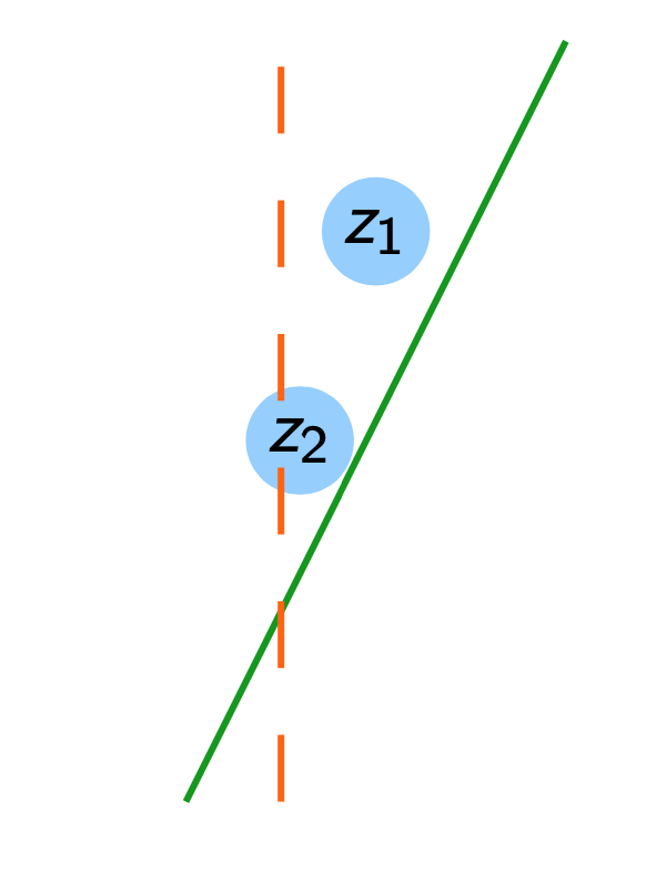
Figure 9: The dotted line is the hypothesis $h$, and the solid line, the target $c$. The adversary has precision $\tau$. The shaded regions represent the set $B_{\tau}(z_{i})$. The counterexample $z_{1}$ is valid as $c$ and $h$ disagree on all of $B_{\tau}(z_{1})$ and both functions are constant in this region, but $z_{2}$ is not as $c$ and $h$ agree on part of $B_{\tau}(z_{2})$.

Definition 6.20 (Precision-Bounded Adversary).

Let $(\mathcal{X},d)$ be a metric space, and let an adversary $\mathbb{A}$ have budget $\rho$. We say that $\mathbb{A}$ is precision-bounded by $\tau$, if for target $c$, hypothesis $h$, and input $x$, $\mathbb{A}$ can only return counterexamples $z\in B_{\rho}(x)$ such that $h$ and $c$ are both constant and disagree on the whole region $B_{\tau}(z)$ and $B_{\tau}(z)\subseteq B_{\rho}(x)$.

Comparison with online learning.

Note that if we set $\rho$ to be large enough so that the perturbation region is the whole instance space $\mathcal{X}$ for any point $x$ (more generally, $\mathcal{U}(x)=\mathcal{X}$), we (almost) recover the adversary model in the online learning setting. The only distinction is that, in online learning, at a given time $t$ the learner is a point $x_{t}$ to classify (implicitly classifying the whole region $B_{\tau}(x_{t})$ in our precision-bounded setting), rather than committing to a hypothesis $h$ on the whole instance space. The adversary (or “nature” if a target must be chosen a priori) reveals the true label after a prediction is made.

In the mistake-bound model, the only constraint is that there exists a concept in $\mathcal{H}$ that is consistent with the labelled sequence $(x_{1},y_{1},),\dots,(x_{t},y_{t})$ seen so far. When working with a precision-bounded adversary, we are implicitly asking the adversary to not give counterexamples too close to the boundary. Then, in the mistake-bound model, this translates into the adversary giving a point $x_{t}$ to predict such that there does not exist time steps $t^{\prime},t^{\prime\prime}$ where $y_{t^{\prime}}\neq y_{t^{\prime\prime}}$ and $B_{\tau}(x_{t^{\prime}})$ and $B_{\tau}(x_{t^{\prime\prime}})$ both intersect with $B_{\tau}(x_{t})$, hence a margin. Margin-based complexity measures for online learning adapted from Ben-David et al., (2009) will be used in this section.

A subtle distinction between the definitions we give below and that of Ben-David et al., (2009) is that the latter defined margin-based Littlestone trees and Littlestone dimension for margin-based hypothesis classes. They require that the hypothesis class $\mathcal{H}$ satisfies the following: for all $h\in\mathcal{H}$, $h$ is of the form $\mathcal{X}\rightarrow\mathbb{R}$, and the prediction rule is

$$\phi(h(x))=\frac{\text{sgn}(h(x))+1}{2}\enspace,$$ (29)

where the magnitude $\left|h(x)\right|$ is the confidence in the prediction. The $\mu$-margin-mistake on an example $(x,y)$ is defined as

$$\left|h(x)-y\right|_{\mu}=\begin{cases}0&\text{if }\phi(h(x))=y\wedge\left|h(x)\right|\geq\mu\\ 1&\text{otherwise}\end{cases}\enspace.$$ (30)

For us, since it is the adversary that is bounded in its precision, we instead consider any hypothesis class where the concepts are boolean functions whose domain is a metric space $(\mathcal{X},d)$. Rather than having the condition $\left|h(x)\right|\geq\mu$ from Equation 30, we encode a margin representing the precision $\tau$ by the requirement that hypotheses must be constant in the $\tau$-expansion around any point in the Littlestone trees. This difference is not only stylistic, but also concerns the semantics of the margin. Our definition moreover implies a uniform margin on the instance space, while the one from Ben-David et al., (2009) can fluctuate in the instance space based on the classifier’s confidence. However, the tools and techniques used here don’t differ much in essence from the ones in Ben-David et al., (2009). The main novelty is the meaning of the notion of margin and its study in the context of robust learning.

Definition 6.21 (Littlestone Trees of Precision $\tau$).

A Littlestone tree of precision $\tau$ for a hypothesis class $\mathcal{H}$ on metric space $(\mathcal{X},d)$ is a complete binary tree $T$ of depth $d$ whose internal nodes are instances $x\in\mathcal{X}$. Each edge is labelled with $-$ or $+$ and corresponds to the potential labels of the parent node $x$ and the region $B_{\tau}(x)$. Each path from the root to a leaf must be consistent with some $h\in\mathcal{H}$, i.e. if $x_{1},\dots,x_{d}$ with labellings $y_{1},\dots,y_{d}$ is a path in $T$, there must exist $h\in\mathcal{H}$ such that $h|_{B_{\tau}(x_{i})}=y_{i}$ for all $i$.

While it is possible to have a hypothesis giving different labels to points in the region $B_{\tau}(x)$ in the standard setting, in the above construction, one must commit to labelling the whole region $B_{\tau}(x)$ either positively or negatively.

For the remainder of the text, we will identify each leaf in a Littlestone tree $T$ with a hypothesis $h\in\mathcal{H}$ that is consistent with the labellings along the path from the root to this leaf. Note that the choice of labelling $y$ of $B_{\tau}(x)$ of some $x\in T$ implies that, in contrast to the standard Littlestone trees, any $h\in\mathcal{H}$ with $h(x)=y$ that is not constant on $B_{\tau}(x)$ cannot be consistent with any path in $T$. The set of consistent hypotheses on $T$ thus does not form a partition of $\mathcal{H}$ in our precision-bounded setting.

We now remark that, by definition, no node in the tree has a $\tau$-expansion that overlaps with the $\tau$-expansion of any of its ancestors.

Proposition 6.22.

Let $T$ be a Littlestone tree of precision $\tau$. Then for any node $x\in T$ and ancestor $x^{\prime}\in T$ of $x$, $B_{\tau}(x)\cap B_{\tau}(x^{\prime})=\emptyset$.

Proof.

Take two paths from the root to two distinct leaves, $h_{0}$ and $h_{1}$, respectively. Let the paths branch off at $x\in T$, with $h_{y}$ giving label $y$ to the whole region $B_{\tau}(x)$. Let $x^{\prime}$ be an ancestor of $x$ in $T$, and note that $h_{0}=h_{1}=b$ on $B_{\tau}(x^{\prime})$ for some $b\in\{0,1\}$. Then, since $h_{0}$ and $h_{1}$ must disagree on all of $B_{\tau}(x)$, it follows that $B_{\tau}(x)\cap B_{\tau}(x^{\prime})=\emptyset$. ∎

We can now define the following variant of the Littlestone dimension, which is analogous to the margin-based Littlestone dimension of Ben-David et al., (2009).

Definition 6.23 (Precision-Bounded Littlestone Dimension).

The Littlestone dimension of precision $\tau$ of a hypothesis class $\mathcal{H}$ on metric space $(\mathcal{X},d)$, denoted $\mathsf{Lit}_{\tau}(\mathcal{H})$, is the depth $k$ of the largest Littlestone tree with bounded precision $\tau$ for $\mathcal{H}$. If no such $k$ exists then $\mathsf{Lit}(\mathcal{H})=\infty$.

Note that setting $\tau=0$, i.e., there are no constraints on the nodes, we recover the Littlestone tree and Littlestone dimension definitions. As an example, let us consider the class of threshold functions, which, when $\tau=0$, have infinite Littlestone dimension.

Proposition 6.24.

Let $\tau>0$. The class $\mathsf{THRESHOLDS}_{B}$ of threshold functions on $[0,B]$ induce Littlestone trees of precision $\tau$ of depth bounded by $log\frac{B}{\tau}-1$. Thus $\mathsf{Lit}_{\tau}(\mathsf{THRESHOLDS}_{B})=\lfloor\log\frac{B}{\tau}-1\rfloor$.

Proof.

Let $\tau>0$ be arbitrary. Here, the optimal strategy to construct a Littlestone tree is to divide the interval $[0,B]$ in two equal parts at each round. Given $x\in[0,B]$ and $\alpha<\alpha^{\prime}\in\mathbb{R}$, in order to have two threshold functions $h_{\alpha}(x)=\mathbf{1}[x\geq\alpha]$ and $h_{\alpha^{\prime}}(x)=\mathbf{1}[x\geq\alpha^{\prime}]$ that disagree on the whole range $[x-\tau,x+\tau]$, we need both $\alpha<x-\tau$ and $\alpha^{\prime}\geq x+\tau$. Thus, at depth $d$, we have divided $[0,B]$ into $2^{d}$ parts we must have $2\tau\geq B2^{-d}$, implying $\mathsf{Lit}_{\tau}(\mathsf{THRESHOLDS}_{B})=\lfloor\log\frac{B}{\tau}-1\rfloor$. ∎

We now show a lower bound on the number of mistakes of any learner against an adversary with bounded precision $\tau$. The proof is identical to the regime $\tau=0$.

Theorem 6.25.

Any online learning algorithm for $\mathcal{C}$ has mistake bound $M\geq\mathsf{Lit}_{\tau}(\mathcal{C})$ against a $\tau$-precision-bounded adversary.

Proof.

Let $\mathcal{A}$ be any online learning algorithm for $\mathcal{C}$. Let $T$ be a Littlestone tree of bounded precision $\tau$ and depth $\mathsf{Lit}_{\tau}(\mathcal{C})$ for $\mathcal{C}$. Clearly, an adversary can force $\mathcal{A}$ to make $\mathsf{Lit}_{\tau}(\mathcal{C})$ mistakes by sequentially and adaptively choosing a path in $T$ in function of $\mathcal{A}$’s predictions. ∎

Now, let us consider a version of the SOA where the adversary has precision $\tau$. The algorithm is identical to the SOA (see Algorithm 5 in Chapter 3), except for the definition of $V^{(b)}_{t}$, which requires that the hypotheses are constant in the region around the prediction.

Algorithm 6 Precision-Bounded Standard Optimal Algorithm

A hypothesis class $\mathcal{\mathcal{H}}$

for $t=1,2,\dots$ do

     $V_{1}\leftarrow\mathcal{H}$

     Receive example $x_{t}$

     $V^{(b)}_{t}\leftarrow\left\{h\in V_{t}\;|\;h|_{B_{\tau}(x_{t})}=b\right\}$

     $\hat{y_{t}}=\underset{b}{\arg\max}\;\mathsf{Lit}_{\tau}\left(V^{(b)}_{t}\right)$

     Receive true label $y_{t}$

     $V_{t+1}\leftarrow V^{(y_{t})}_{t}$

end for

Below, we show that this slight modification of the SOA is also optimal for cases in which the adversary is constrained by $\tau$. This is analogous to Theorem 21 in (Ben-David et al.,, 2009), who did not include the proof of optimality for brevity. We have included it in this thesis for completeness.

Theorem 6.26.

The precision-bounded Standard Optimal Algorithm makes at most $\mathsf{Lit}_{\tau}(\mathcal{C})$ mistakes in the mistake-bound model of online learning when the adversary has precision $\tau$.

Proof.

We will show that, at every mistake, the precision-bounded Littlestone dimension of the subclass $V_{t}$ decreases by at least 1 after receiving the true label $y_{t}$.

WLOG, assume that there does not exist $t^{\prime}<t$ such that $x_{t^{\prime}}\in B_{\tau}(x_{t})$, as otherwise this implies that $V_{t}^{(y_{t^{\prime}})}=V_{t}$ and $V_{t}^{(\neg y_{t^{\prime}})}=\emptyset$, and we cannot make a mistake (note in particular that we cannot have two differently labelled points in $B_{\tau}(x_{t})$ as otherwise this would not be a valid example for the adversary to give).

Suppose that, at time $t$, $y_{t}=\arg\min_{b}\mathsf{Lit}_{\tau}(V^{(b)}_{t})$. Note that $V_{t+1}=V^{(y_{t})}_{t}$. Now, consider any two Littlestone trees $T_{y_{t}}$ and $T_{\hat{y}_{t}}$ of precision $\tau$ and maximal depths for $V^{(y_{t})}_{t}$ and $V^{(\hat{y})}_{t}$, respectively. By Proposition 6.22 and definition of $V^{(b)}_{t}$, neither tree can contain nodes whose $\tau$-expansions intersect with $B_{\tau}(x_{t})$. Moreover, all hypotheses in $V^{(y_{t})}_{t}$ and $V^{(\hat{y})}_{t}$ are constant on $B_{\tau}(x_{t})$. Hence it is possible to construct a $\tau$-constrained Littlestone tree $T$ for $V_{t}$ of depth $\min_{b}\mathsf{Lit}_{\tau}(V^{(b)}_{t})+1$ (recall that $T$ must be complete). Then $\mathsf{Lit}_{\tau}(V_{t})\geq\mathsf{Lit}_{\tau}(V^{({y_{t}})}_{t})+1=\mathsf{Lit}_{\tau}(V_{t+1})+1$, as required. ∎

Remark 6.27.

When considering threshold functions on $[0,1]$, and given example $x_{t}$ to predict, the SOA’s strategy is effectively to look at the labelled points in the history and consider the largest $x^{(0)}\in[0,1]$ with negative label and the smallest $x^{(1)}\in[0,1]$ with positive label, and predict $y_{t}=\underset{b}{\arg\min}\left|x_{t}-x^{(b)}\right|$.

We now turn our attention to the robust learning of halfspaces in $(\mathbb{R}^{n},d_{2})$ against adversaries of precision $\tau$, where $d_{2}$ is the metric induced by the $\ell_{2}$ norm. As pointed out by Ben-David et al., (2009), we essentially have the same argument as the Perceptron algorithm, because, once the hypothesis is sufficiently close to the target, the adversary cannot return counterexamples near the boundary. Note that this result can be generalized to $\ell_{p}$ norms. Figure 10 depicts the argument of the proof of Theorem 6.28.

Theorem 6.28.

Fix constants $B,\tau>0$. Let the adversary’s budget $\rho$ be measured by the $\ell_{2}$ norm. Let $\mathsf{LTF}_{\mathbb{R}^{n}}$ be the class of halfspaces on $\mathbb{R}^{n}$ where the instance space is restricted to points $x\in\mathbb{R}^{n}$ with $\left\|x\right\|_{2}\leq B-\rho$. Then, $\mathsf{LTF}_{\mathbb{R}^{n}}$ is distribution-free $\rho$-robustly learnable against an adversary of precision $\tau$ using the $\mathsf{EX}$ and $\rho$-$\mathsf{LEQ}$ oracles with sample complexity $m(n,\epsilon,\delta)=O(\frac{1}{\epsilon}(n^{3}+\log(1/\delta)))$ and query complexity $r(n,\epsilon,\delta)=m(n,\epsilon,\delta)\cdot\frac{B^{2}}{\tau^{2}}$. Note that this is query-efficient if $\frac{B^{2}}{\tau^{2}}=\text{poly}(n)$.

Note that the dependence on $\tau$ in the mistake bound, and thus the $\mathsf{LEQ}$ upper bound, is $1/\tau^{2}$, in contrast to the dependence of $\log 1/\tau$ for thresholds.

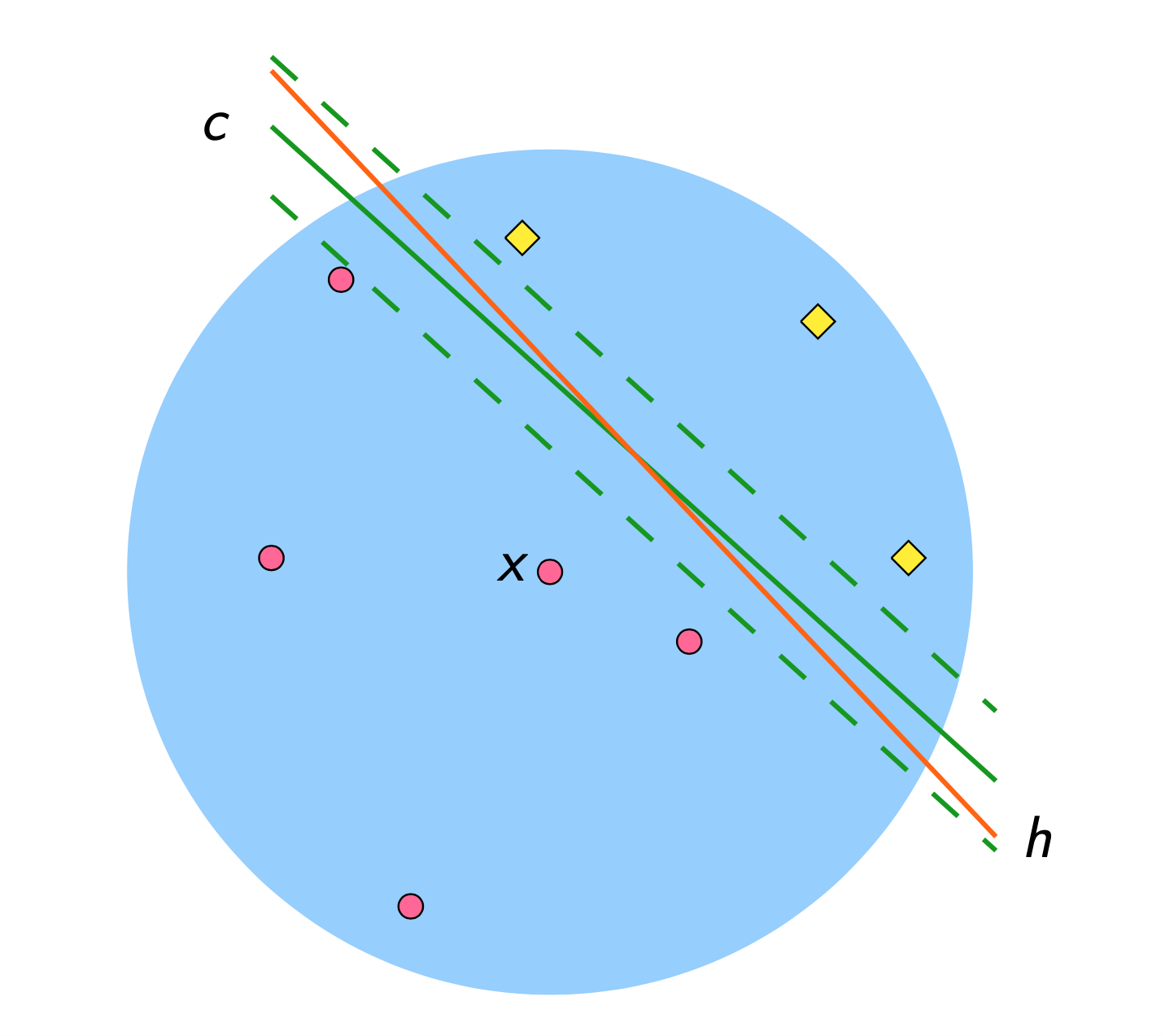
Figure 10: A visual representation of the proof of Theorem 6.28. The dotted lines on either side of the target $c$ represent a margin of $\tau/2$. Any hypothesis within the dotted lines in the (shaded) perturbation region ensures that an adversary of bounded precision $\tau$ cannot return any counterexamples. Finally, counterexamples must be labelled according to the target $c$, and both $h$ and $c$ are not constant on $B_{\rho}(x)$.

Proof.

The sample complexity follows from Theorem 6.15. The query upper bound follows from Lemma 6.11 and the mistake bound for the Perceptron algorithm (see Theorem 3.16). To see that the bound for Perceptron can be used, note that the adversary having precision $\tau$ implies that any consistent target function $c(x)=a^{\top}x+a_{0}$ and any counterexample $z$ will satisfy the conditions (i) $\left\|z\right\|_{2}\leq B$ and (ii) $\tau\leq\frac{c(z)(a^{\top}z)}{\left\|z\right\|_{2}}$ from Theorem 3.16. ∎

22 Lower Bounds on Robust Learning with $\mathsf{LEQ}$

In this section, we derive lower bounds on the expected number of queries of robust learning algorithms for various concept classes. We start with general lower bounds and conclude by looking at specific concept classes.

22.1 General Query Complexity Lower Bounds

We start by giving a general lower bound on the query complexity of the $\mathsf{LEQ}$ oracle that is linear in the restricted Littlestone dimension of a concept class. This notion, which restricts the region of the instance space where the nodes in the Littlestone tree can come from, will be defined below, along with the restricted VC dimension.

We first define the notion of the restricted VC dimension of a concept class. We note that we can straightforwardly extend the definitions below to an arbitrary perturbation region $\mathcal{U}:\mathcal{X}\rightarrow 2^{\mathcal{X}}$, and obtain analogous results.

Definition 6.29 ($\rho$-restricted VC Dimension).

The $\rho$-restricted VC dimension of a concept class $\mathcal{C}$, denoted $\mathsf{VC}|_{\rho}(\mathcal{C})$, is the size $d$ of the largest set $X\subseteq\mathcal{X}$ shattered by $\mathcal{C}$ such that there exists $x^{*}\in X$ where $x\in B_{\rho}(x^{*})$ for all $x\in X$.

We now introduce the restricted Littlestone dimension.

Definition 6.30 ($\rho$-restricted Littlestone Dimension).

The $\rho$-restricted Littlestone dimension of a hypothesis class $\mathcal{H}$, denoted $\mathsf{Lit}|_{\rho}(\mathcal{H})$, is the depth $d$ of the largest Littlestone tree $T$ for $\mathcal{H}$ with root node $x^{*}$ such that $x\in B_{\rho}(x^{*})$ for all the nodes $x\in T$.

Remark 6.31.

It follows from the upper bound on the (standard) VC dimension by the Littlestone dimension that $\mathsf{VC}|_{\rho}(\mathcal{C})\leq\mathsf{Lit}|_{\rho}(\mathcal{H})$, as we can construct a restricted Littlestone tree from a witness set of the restricted VC dimension.

We are now ready to state the main theorem of this section.

Theorem 6.32.

Let $\mathcal{C}$ be a concept class of $\rho$-restricted Littlestone dimension $\mathsf{Lit}|_{\rho}(\mathcal{C})=d$. Then there exists a distribution on $\mathcal{X}$ such that any $\rho$-robust learning algorithm for $\mathcal{C}$ has an expected number of queries $\Omega(d)$ to the $\rho$-$\mathsf{LEQ}$ oracle.

As a consequence of Remark 6.31, we have the following corollary.

Corollary 6.33.

Let $\mathcal{C}$ be a concept class of $\rho$-restricted VC dimension $\mathsf{VC}|_{\rho}(\mathcal{C})=d$. Then there exists a distribution on $\mathcal{X}$ such that any $\rho$-robust learning algorithm for $\mathcal{C}$ has an expected number of queries $\Omega(d)$ to the $\rho$-$\mathsf{LEQ}$ oracle.

The proof of Theorem 6.32 is similar to showing that a mistake lower bound in online learning can be transformed in an expected mistake lower bound when we instead require the adversary to choose a label before a (potentially randomized) prediction is made.

In order to prove Theorem 6.32, we will use Yao’s minimax principle, which will allow us to give lower bounds for randomized algorithms while only considering deterministic algorithms in our analysis.

We will start with some notation. Let $\text{cost}(A,z)$ represent the real-valued cost of an algorithm $A$ on an input $z$ for problem $P$ (e.g., running time, number of queries, etc.). For a distribution $\mathcal{D}$ on the set $Z$ of potential inputs to $P$, the cost of $A$ on $\mathcal{D}$ is defined as $\text{cost}(A,\mathcal{D}):=\underset{{z\sim\mathcal{D}}}{\mathbb{E}}\left[\text{ cost}(A,z)\right]$. The distributional complexity of $P$ is $\underset{\mathcal{D}}{\max}\;\underset{A\in\mathcal{A}}{\min}\text{ cost}(A,\mathcal{D})$ (the cost of the worst distribution on inputs for the best deterministic algorithm). Now, as we can see a randomized algorithm $R$ as a distribution $\mathcal{R}$ over all the possible deterministic algorithms, we can define the cost of a randomized algorithm as cost$(R,x)=\text{ cost}(\mathcal{R},x)=\underset{{A\sim\mathcal{R}}}{\mathbb{E}}\left[\text{ cost}(A,x)\right]$. The randomized complexity of $P$ is defined as $\underset{\mathcal{R}}{\min}\;\underset{x}{\max}\text{ cost}(R,x)$.

Yao’s minimax principle states that the randomized complexity and distributional complexity of a problem $P$ are equal, i.e.,

$$\underset{\mathcal{R}}{\min}\;\underset{x}{\max}\text{ cost}(\mathcal{R},x)=\underset{\mathcal{D}}{\max}\;\underset{A\in\mathcal{A}}{\min}\text{ cost}(A,\mathcal{D})\enspace.$$

For us, the input to the learning problem will be the target concept, and as such the distribution $\mathcal{D}$ will be over the concept class $\mathcal{C}$. The cost of an algorithm $A$ on $c$ is the number of queries to the $\rho$-$\mathsf{LEQ}$ oracle, and we are interested in the expected number of counterexamples returned.

Proof of Theorem 6.32.

The idea behind the proof is to choose a distribution in which all the elements of the Littlestone tree appear in the perturbation region of its root. We then derive query lower bounds for deterministic algorithms and a deterministic $\mathsf{LEQ}$. We finally use Yao’s minimax principle to lower bound the number of queries of any robust learning algorithm to the $\mathsf{LEQ}$ oracle.

Distribution on $\mathcal{X}$. Let $T$ be a Littlestone tree of depth $d$ with root $x^{*}\in X$ such that all its nodes are contained in $B_{\rho}(x^{*})$. Let $D$ be a distribution on $\mathcal{X}$ be such that $D(x^{*})=1$. Hence, any query to $\mathsf{EX}(c,D)$ will return $(x^{*},c(x^{*}))$. Moreover, any learning algorithm must be exact on $B_{\rho}(x^{*})$, as otherwise the existence of a point $z$ in $B_{\rho}(x^{*})$ such that the target and hypothesis disagree results in the robust risk being 1.

Let $\widetilde{\mathcal{C}}=\left\{c_{1},\dots,c_{2^{d-1}}\right\}$ be the set of concepts appearing as leaves of the subtree $T^{\prime}$ of $T$ that label ${x^{*}}$ positively. We will pick the target $c$ at random from $\widetilde{\mathcal{C}}$.

$\mathsf{LEQ}$ strategy. Let the $\rho$-$\mathsf{LEQ}$ oracle have access to $T$ as its internal ordering. Upon being queried with $(x^{*},h)$, $\mathsf{LEQ}$ returns a counterexample $x^{\prime}$ of least depth. Namely, a target $c\in\widetilde{\mathcal{C}}$ determines a path from $x^{*}$ to a leaf, and the $\mathsf{LEQ}$ oracle returns the highest node where $h$ and $c$ disagree.

Deterministic algorithms. In order to use Yao’s minimax principle, we first consider a set of deterministic algorithms. For any fixed distribution $\mathcal{D}$ on the target concepts, a learning algorithm $A$ achieving $\underset{A\in\mathcal{A}}{\min}\text{ cost}(A,\mathcal{D})$ must be consistent with the data seen so far. Otherwise, $\mathsf{LEQ}$ can simply return a counterexample that has already been returned, increasing the number of queries to $\mathsf{LEQ}$.

Without loss of generality, we consider the setting where the Littlestone tree $T$ the $\mathsf{LEQ}$ uses to return counterexamples is known to $A$. This implies that if $A$ receives $(x_{i},c(x_{i}))$ as a counterexample, then there exists a unique path from $x^{*}$ to a node containing $x_{i}$ where parents nodes of $x_{i}$ must have been labelled correctly by the hypothesis. Any algorithm that does not know this information (or doesn’t use it) is dominated by an algorithm knowing this information. Then any $A$ achieving $\underset{A\in\mathcal{A}}{\min}\text{ cost}(A,\mathcal{D})$ in this setting must be consistent on the counterexamples and (implicitly revealed) correctly labelled points.

Executions paths. Consider a given deterministic algorithm $A$ that is consistent with the data seen so far. After seeing $(x^{*},+1)$, $A$ returns a hypothesis $h_{1}$, thus the label $h_{1}(x_{1})$ is fixed (where $x_{1}$ is the child of $x^{*}$ with a positively labelled edge). Then, one of the edges coming out of the node $x_{1}$ will be correct, while the other will be incorrect. Since each concept in $\widetilde{\mathcal{C}}$ defines a path in $T^{\prime}$ and $A$ is deterministic, for each node $x$ in $T^{\prime}$, one of its edges is correct and the other, incorrect. Then, for each leaf $c$ in $T^{\prime}$, the edges from $x_{1}$ to $c$ that are marked as incorrect represent the counterexamples given to $A$ by $\mathsf{LEQ}$ if $c$ were the target. It is then easy to see that choosing the target u.a.r. from the leaves $\widetilde{\mathcal{C}}$ of $T’$, we have an expected number of counterexamples that is exactly $(d-1)/2$. Thus

$$\underset{\mathcal{D}}{\max}\;\underset{A\in\mathcal{A}}{\min}\text{ cost}(A,\mathcal{D})\geq\underset{A\in\mathcal{A}}{\min}\text{ cost}(A,U(\widetilde{\mathcal{C}}))\geq\frac{d-1}{2}\enspace,$$

where $U(\widetilde{\mathcal{C}})$ is the uniform distribution on $\widetilde{\mathcal{C}}$. In fact, we can see that the distribution achieving the maximum on the LHS is the uniform distribution on $\widetilde{\mathcal{C}}$.

Putting it all together. Now, any learning algorithm in this setting is either deterministic or randomized. If the algorithm is randomized, it can be expressed as a distribution on the set of deterministic algorithms. We can thus apply Yao’s principle and get that there exists a distribution on $\mathcal{X}$ such that any robust learning algorithm for $\mathcal{C}$ will have an expected number of queries to $\mathsf{LEQ}$ that is linear in the restricted Littlestone dimension of $\mathcal{C}$. ∎

22.2 Bounds on the Restricted VC and Littlestone Dimensions

In this section, we study bounds on the restricted VC and Littlestone dimensions of monotone conjunctions, decision lists and linear classifiers. This enables us to use Theorem 6.32 to get lower bounds on the expected number of queries to $\mathsf{LEQ}$ for the robust learning of these classes. The VC dimension bounds are (asymptotically) the same as the standard VC dimension for these classes. We finish by showing this is not always the case, and exhibiting an example where the VC dimension is not a lower bound for the expected number of queries to $\mathsf{LEQ}$, hence justifying the use of alternative complexity measure in our setting.

We summarize our results on the restricted VC dimension in Table 3. The proofs of the bounds appear in Appendix 9.C. As corollaries of Theorem 6.32, we get that the restricted VC dimension lower bounds presented in Table 3 are lower bounds on the expected number of queries to the $\mathsf{LEQ}$ oracle.

Concept Class	$\mathsf{VC}$ dimension	$\rho$-restricted $\mathsf{VC}$ dimension
Conjunctions	$n$	$2$ (if $\rho=1$) $n$ (if $\rho\geq 2$)
Linear Threshold Functions	$n+1$	$n+1$
$k$-Decision Lists	$\widetilde{\Theta}(n^{k})$	$\widetilde{\Theta}(n^{k})$ (given $\rho\geq k$)

Table 3: Comparing the VC dimension and the $\rho$-restricted VC dimension for given concept classes. The $\widetilde{\Theta}$ notation hides the logarithmic factors. Unless otherwise stated, we assume $\rho\geq 1$.

Now, while linear classifiers in $\mathbb{R}^{n}$ have a (restricted) VC dimension of $n+1$, their $\rho$-restricted Littlestone dimension is infinite. Indeed, it suffices to consider the subclass of thresholds (for which the proof of its Littlestone dimension being infinite can easily be adapted to the restricted setting) giving the lemma below.

Corollary 6.34.

Given $\rho>0$, there exists a distribution on $\mathbb{R}^{n}$ such that any $\rho$-robust learning algorithm for linear classifiers has an infinite expected number of queries to $\rho$-$\mathsf{LEQ}$.

We now turn our attention to the relationship between VC dimension and its restricted counterpart, and their use for $\mathsf{LEQ}$ lower bounds.

In general, is $\mathsf{VC}|_{\rho}(\mathcal{H})=\widetilde{\Theta}(\mathsf{VC}(\mathcal{H}))$?

No: we exhibit a concept class $\mathcal{H}$ where $\mathsf{VC}(\mathcal{H})=d$ but $\mathsf{VC}|_{\rho}(\mathcal{H})=1$. This shows that there can be an arbitrary gap between the restricted VC dimension and its standard counterpart. Let $X=\left\{x_{1},\dots,x_{d}\right\}$ be a set of $d$ points on $\left\{0,1\right\}^{n}$ whose balls of radius $\rho$ don’t coincide (choose $\rho$ and $d$ as functions of $n$ such that this is possible). Define the following concept class $\mathcal{C}=\bigcup_{S\subseteq X}\left\{c(x)=\mathbf{1}[x\in S]\right\}$. Clearly, $\mathsf{VC}(\mathcal{C})=d$, but $\mathsf{VC}|_{\rho}(\mathcal{C})=1$.

Are there better $\mathsf{LEQ}$ lower bounds than $\mathsf{VC}|_{\rho}$?

Yes: we can still show an expected query lower bound of $\Omega(d)$ in the example above by constructing a uniform distribution on some set $X^{*}=\left\{x_{1}^{*},\dots,x_{d}^{*}\right\}$ such that $X\cap X^{*}=\emptyset$ and $x_{i}^{*}\in B_{\rho}(x_{i})$ for all $i$, implying that $c(x_{i})=0$ for all $1\leq i\leq d$ and $c\in\mathcal{C}$. Thus, to get a hypothesis with robust risk strictly smaller than $1/d$, exact learning is required. We can show that, by choosing the target at random from $\mathcal{C}$, the expected number of counterexamples for any algorithm is lower bounded by a function $\Omega(d)$ with the same reasoning as the proof of Theorem 6.32.

Is the VC dimension a general lower bound for $\mathsf{LEQ}$?

No: consider the problem defined above, but with the perturbation region being the identity function for each $x\in X$. Clearly, it is not possible to construct the distribution in the previous example. In fact, a random sample of size $\Theta(d)$ is sufficient to guarantee generalization, without the use of queries.

23 Further Comparing the Local Query Models

We finish this chapter by drawing a more nuanced picture of the local membership and equivalence query frameworks, in how they compare with each other (Section 23.1) and to other active learning set-ups (Section 23.2).

23.1 Local Membership and Equivalence Queries

We start by showing two results on the efficient robust learnability of singletons. The first result is a negative one: singletons are not efficiently robustly learnable in the distribution-free setting in the $\mathsf{EX}$+$\mathsf{LMQ}$ model. However, the second result shows that it is possible to do so in the $\mathsf{EX}$+$\mathsf{LEQ}$ model when the perturbation budget $\rho$ and the locality radius $\lambda$ are equal. While simple, together these results highlight the relevance of the $\mathsf{LEQ}$ oracle in robust learning. Indeed, they show that, unlike in the standard PAC model, membership queries cannot, in general, simulate equivalence queries in the robust learning setting. In robust learning, because of the existence of the existential quantifier in the robust loss, $\mathbf{1}[\exists z\in B_{\rho}(x)\;.\;c(z)\neq h(z)]$, polynomially-many (local) membership queries cannot in general suffice to estimate the robust loss, as illustrated below. We finish by looking at parities, a concept class for which local membership and equivalence queries are equally powerful.

We first start by showing that having access to local membership queries does not ensure the robust learnability of singletons in the distribution-free setting regardless of the query radius.

Proposition 6.35.

If $\rho$ is $\omega(1)$, the class of singletons is not efficiently $\rho$-robustly learnable in the distribution-free setting when the learner has access to a $\lambda$-$\mathsf{LMQ}$ oracle for any $\lambda$.

Proof.

Fix $x\in\mathcal{X}$ and consider the distribution $D$ on $\mathcal{X}$ such that $D(x)=1$. We distinguish two cases. If $\lambda<\rho$, it suffices to choose two singletons in $B_{\rho}(x)\setminus B_{\lambda}(x)$ and draw the target concept uniformly at random between them (the learner cannot query a positive label, and cannot do better than choosing the right target at random). The second case is $\lambda\geq\rho$. Note that $\left|B_{\rho}(x)\right|\geq(n/\rho)^{\rho}$, which is superpolynomial in $n$ for any budget $\rho=\omega(1)$ (as $\rho\leq n$). Now, for any LMQ strategy with a polynomial query upper bound $r(n)$, there exists a sufficiently large input dimension $N$ such that, after $r(N)$ queries, at least half the points in $B_{\rho}(x)$ have yet to be queried. Choosing a target uniformly at random in $B_{\rho}(x)\setminus\left\{x\right\}$, using Lemma 4.9, and noting that any two singletons in $B_{\rho}(x)$ have robust risk of 1 against each other, suffices to lower bound the expected risk of any hypothesis over the choice of the target concept by a constant. ∎

We now show that, in contrast, having access to a local equivalence query oracle enables the robust learnability of singletons in the distribution-free setting.

Proposition 6.36.

Singletons are efficiently distribution-free $\rho$-robustly learnable given a $\rho$-$\mathsf{LEQ}$ oracle.

Proof.

Draw a sufficiently large sample $S\sim D^{m}$ to ensure robust generalization, as in Lemma 6.6 ($\left|S\right|$ is polynomial in the input dimension $n$ and learning parameters). If there exists a positively labelled point $x\in S$, we have learned the target singleton. Otherwise, query the $\mathsf{LEQ}$ oracle with the constant function 0 on the points in $S$ until we receive a counterexample (the target singleton) or until it is confirmed that all points have robust loss of 0. In either case, we have queried at most $m$ points and the hypothesis is robustly consistent with the training sample, and we are done. ∎

Note that this is in contrast with the fact that, if a concept class is exactly learnable with access to the $\mathsf{MQ}$ and $\mathsf{EQ}$ oracles, then it is PAC learnable with random examples and access to $\mathsf{MQ}$ (see Section 6.5 for details). Fundamentally, the existential quantifier in the robust risk definition renders simulating the $\mathsf{LEQ}$ oracle with the $\mathsf{LMQ}$ oracle impossible.

Learning parities with $\mathsf{LMQ}$ and $\mathsf{LEQ}$.

There are cases where the $\mathsf{EX}$+$\mathsf{LMQ}$ and $\mathsf{EX}$+$\mathsf{LEQ}$ models are equally powerful. Indeed, it is easy to see that access to the 1-$\mathsf{LMQ}$ or 1-$\mathsf{LEQ}$ oracle is sufficient to exactly learn parities with one query to $\mathsf{EX}$. For the former case, it suffices to flip each bit $i$ of an instance $x$ drawn from $\mathsf{EX}$ and give $x\oplus e_{i}$ to the $\mathsf{LMQ}$ oracle to observe whether $i$ is in the target parity. For the latter, note that each counterexample $(x,y)$ is linearly independent from the set of data points already collected, so there must be at most $n$ counterexamples in $B_{1}(x)$, thus exactly identifying the target parity.

23.2 A Two-Way Separation between $\mathsf{LEQ}$ and $\mathsf{EQ}$

In this section, we compare local and “global” query oracles. We show that, when considering robust learning, the $\mathsf{EX}$+$\mathsf{LEQ}$ and $\mathsf{EX}$+$\mathsf{EQ}$ models are in general incomparable. This is in contrast with $\mathsf{LMQ}$ and $\mathsf{MQ}$, where a learning algorithm with access to $\mathsf{LMQ}$ can straightforwardly be simulated by an algorithm with access to $\mathsf{MQ}$.

We first show the existence of a robust learning problem on $\left\{0,1\right\}^{n}$ such that the $\mathsf{EX}$+$\mathsf{LEQ}$ model requires one sample point from $\mathsf{EX}$ and one query to $\mathsf{LEQ}$, while it requires $\log n$ calls to $\mathsf{EQ}$ in the $\mathsf{EX}$+$\mathsf{EQ}$ model. We then show the existence of a robust learning problem on $\left\{0,1\right\}^{n}$ such that the $\mathsf{EX}$+$\mathsf{LEQ}$ model requires $O(1/\epsilon)$ sample points from $\mathsf{EX}$ and a total of $1/\epsilon$ queries to $\mathsf{LEQ}$ in order to have a robust error bounded by $\epsilon$, while it only requires a single call to $\mathsf{EQ}$ in the $\mathsf{EX}$+$\mathsf{EQ}$ model.

We now formally state the result showing that (perhaps counter-intuitively) 1-$\mathsf{LEQ}$ can sometimes be more powerful than $\mathsf{EQ}$. The idea is to create a learning problem such that any counterexample in a ball of radius one around a point reveals full information about the target, but when the oracle is free to choose any point in the input space, it can (adversarially) reveal partial information. To simplify our analysis, we will assume that the oracle does not have to commit to any target, as long as the target is defined on the support of the distribution (in order to have a well-defined example oracle). The target is not necessarily defined on the rest of the input space, only restricting the oracle to output a sequence of counterexamples for which there always exists a consistent concept. As mentioned earlier in this chapter, choosing a target a priori (i.e., similarly to the online stochastic setting) simply results in expected bounds of the same order as if the oracle does not have to commit to a target (i.e., the mistake-bound online setting).

Theorem 6.37.

Let $\mathcal{C}=\left\{x\mapsto x_{i}\;|\;i\in[n]\right\}$ be the class of monotone dictators. There exists a distribution $D$ on $\left\{0,1\right\}^{n}$ and target concept $c\in\mathcal{C}$ such that 1-robustly learning $(c,D)$ requires at most one query to 1-$\mathsf{LEQ}$, but, for any learning algorithm, at least $\log n$ queries to $\mathsf{EQ}$.

Proof.

Let $D$ be such that $D(\mathbf{0})=1$, and note that robustly learning $\mathcal{C}$ against an adversary with budget 1 requires exact learning. Moreover, the labelled instance $(\mathbf{0},0)$ gives no information about the target concept.

For the $\mathsf{LEQ}$ model, the learner samples the point $\mathbf{0}$ from $\mathsf{EX}$, and gives the constant hypothesis $0$ to $\mathsf{LEQ}$. Since the oracle must return $x\in B_{1}(\mathbf{0})$ such that $c(x)=1$, it must return $e_{i}$ such that $c(x)=x_{i}$.

For the $\mathsf{EQ}$ model, the idea is that, for any hypothesis $h$ the learner gives to $\mathsf{EQ}$, the oracle can always find a counterexample that removes at most half of the potential targets. Let $I_{t}=\left\{i\in[n]\;|\;x_{i}\text{ is consistent with the history}\right\}$ be the set of indices (and thus concepts) that are consistent with the sequence of counterexamples given up until query $t$, and note that $I_{1}=[n]$. Let $h\in 2^{\left\{0,1\right\}^{n}}$ be an arbitrary hypothesis and define the following function

$$\#1:(x,I)\mapsto\sum_{i\in I}x_{i}$$

that returns the number of 1’s at the indices of $I\subseteq[n]$ in an instance $x\in\left\{0,1\right\}^{n}$. Define the following instances:

$$x_{*}:=\underset{x:h(x)=1}{\arg\min}\;\#1(x,I_{t})\enspace,$$

$$x^{*}:=\underset{x:h(x)=0}{\arg\max}\;\#1(x,I_{t})\enspace.$$

We now argue that one of $x_{*}$ or $x^{*}$ will decrease $I_{t}$ by at most half. Recall that the oracle’s goal is to reveal as little information as possible to the learner at every query. Note that, given $x\in\left\{0,1\right\}^{n}$, if $h(x)\neq c(x)$, then all the bits with value $c(x)$ are still viable target functions for that counterexample.

Now, if $x^{*}$ is a counterexample, then $c(x^{*})=1$, and there are $\#1(x,I_{t})$ concepts that are still consistent with the counterexample history. Likewise, if if $x_{*}$ is a counterexample, then $c(x^{*})=0$, and there are $\left|I_{t}\right|-\#1(x,I_{t})$ concepts that are still consistent with the counterexample history. Thus, if the oracle chooses the counterexample maximizing the number of consistent concepts with the history, we have that

$$\left|I_{t+1}\right|=\max\left\{\left|I_{t}\right|-\#1(x_{*},I_{t}),\#1(x^{*},I_{t})\right\}\geq\lfloor\left|I_{t}\right|/2\rfloor\enspace,$$

which concludes the proof. ∎

Remark 6.38.

As a corollary of Theorem 6.37, we get that there exists a robust learning problem for which distribution-free efficient robust learning is still possible when $\lambda>\rho$, but where the query complexity is much larger than if $\lambda=\rho$ (set $\rho=1$ in the problem above).

Now, we formally show that, for some learning problems, an $\mathsf{EQ}$ oracle is more powerful than an $\mathsf{LEQ}$ oracle.

Theorem 6.39.

Let $\mathcal{C}=\left\{x\mapsto\mathbf{1}[x=x^{\prime}]\;|\;x^{\prime}\in\left\{0,1\right\}^{n}\right\}$ be the class of singletons. Then there exists a distribution $D$ on $\left\{0,1\right\}^{n}$ and target concept $c\in\mathcal{C}$ such that robustly learning $(c,D)$ requires at most one query to $\mathsf{EQ}$, but, for any learning algorithm, at least $1/\epsilon$ queries to $\lambda$-$\mathsf{LEQ}$ for robust accuracy $\epsilon$.

Proof.

Let $k=\lfloor 1/\epsilon\rfloor$. Let $X=\left\{x_{1},\dots,x_{k}\right\}$ be instances in $\left\{0,1\right\}^{n}$ whose $\lambda$-expansions don’t intersect (let $n$ be sufficiently large and choose $\lambda$ as a function of $n$ and $\epsilon$ so that this is possible). Let $c(x_{i})=0$ for all instances $x_{i}$, and let $D$ be the uniform distribution on $X$. Note that, if the target singleton is in any of the perturbation regions $B_{\rho}(x_{i})$, then a $\rho$-robust learning algorithm given robust accuracy parameter $\epsilon$ must identify the target exactly. Without loss of generality, we let $\rho=\lambda$.

For the $\mathsf{EQ}$ bound, the learner can clearly query $\mathsf{EQ}$ with the constant function $0$, and get the singleton target as a counterexample, without any call to $\mathsf{EX}$.

For the $\lambda$-$\mathsf{LEQ}$ bound, the oracle’s strategy is simply to (adaptively) return that $c=0$ on all queries $(x_{i_{1}},h_{1}),\dots,(x_{i_{k-1}},h_{k-1})$ until the last query $x_{i_{k}}$, which reveals the target singleton. This yields a lower bound of $k$ queries to $\lambda$-$\mathsf{LEQ}$ (the optimal strategy is to not repeat an instance in the queries and always choose $h_{i}=0$) ∎

Remark 6.40.

As the mistake-bound of singletons in online learning is 1, the theorem above also shows that $\rho$-robust learning with a $\rho$-$\mathsf{LEQ}$ can result in query complexity lower bounds that are strictly greater than mistake bounds in online learning. Note though that the optimal algorithm still only makes one mistake, it simply has to query the $\mathsf{LEQ}$ a certain number of times before making it.

24 Summary and Open Problems

In this chapter, we have thoroughly studied the powers and limitations of both local membership and equivalence queries in the context of robust learning. In particular, we have outlined when access to either oracle is necessary to enable robustness guarantees, as well as obtained lower bounds on the local query complexity of various robust learning problems.

24.1 Final Remarks on Local Query Oracles

We discuss the implementation of local query oracles, as well as how the $\mathsf{LMQ}$ and $\mathsf{LEQ}$ oracles differ when considering the constant-in-the-ball notion of robustness.

Implementing $\mathsf{LEQ}$ oracle.

In practice, one always has to find a way to approximately implement oracles studied in theory. A possible way to generate counterexamples with respect to the exact-in-the-ball notion of robustness is as follows. Suppose that there is an adversary that can generate points $z\in B_{\rho}(x)$ such that $h(z)\neq c(z)$. Provided such an adversary can be simulated, there is a way to (imperfectly) implement the $\mathsf{LEQ}$ oracle in practice. Thus, the use of these oracles can be viewed as a form of adversarial training.

Local query analogues for the constant-in-the-ball risk.

Both the $\mathsf{LMQ}$ and $\mathsf{LEQ}$ models are particularly well-suited for the standard and exact-in-the-ball risks, as they address information-theoretic limitations of learning with random examples only. On the other hand, while information-theoretic limitations of robust learning with respect to the constant-in-the-ball notion of robustness arise when the perturbation function $\mathcal{U}$ is unknown to the learner, computational obstacles can also occur even when the definition of $\mathcal{U}$ is available. Indeed, determining whether the hypothesis changes label in the perturbation region could be intractable. In these cases, the Perfect Attack Oracle (PAO) of Montasser et al., (2021) can be used to remedy these limitations for robust learning with respect to the constant-in-the-ball robust risk. Crucially, in their setting, counterexamples could have a different label to the ground truth: a counterexample $z\in\mathcal{U}(x)$ for $x$ is such that $h(z)\neq c(x)$, not necessarily $h(z)\neq c(z)$. A striking example of this is when $\mathcal{U}(x)=\mathcal{X}$. In this case, we only want to know if the hypothesis is constant on the whole input space. This could compromise the standard accuracy of the hypothesis (see e.g., Tsipras et al., (2019) for a learning problem where robustness and accuracy are at odds). Finally, an $\mathsf{LMQ}$ analogue for the constant-in-the-ball risk is not needed: the only information we need for a perturbed point $z\in B_{\rho}(x)$ is the label of $x$ (given by the example oracle) and $h(z)$. Given that one of the requirements of PAC learning is that the hypothesis is efficiently evaluatable, we can easily compute $h(z)$.

Comparison with (Montasser et al.,, 2021).

Closest to our work in this chapter is that of Montasser et al., (2021), who derive sample and PAO query bounds for the realizable constant-in-the-ball setting. They use the algorithm from (Montasser et al.,, 2019) to get a sample complexity of $\tilde{O}\left(\frac{\mathsf{VC}(\mathcal{H}){\mathsf{VC}^{*}}^{2}(\mathcal{H})+\log(1/\delta)}{\epsilon}\right)$ and derive a query complexity of $\tilde{O}(2^{\mathsf{VC}(\mathcal{H})^{2}\mathsf{VC}^{*}(\mathcal{H})^{2}\log^{2}(\mathsf{VC}^{*}(\mathcal{H}))}\mathsf{Lit}(\mathcal{H}))$, where $\mathsf{VC}^{*}(\mathcal{H})$ is the dual VC dimension of a hypothesis class. They also derive query lower bounds: their general PAO query complexity lower bound is $\Omega(\log(\text{Tdim}(\mathcal{H})))$, where $\text{Tdim}(\mathcal{H})$ is the threshold dimension of a hypothesis class. The threshold dimension is bounded below by the logarithm of the Littlestone dimension, hence giving a general query lower bound of $\Omega(\log\log(\mathsf{Lit}(\mathcal{H})))$. Since threshold functions have a threshold dimension exponential in the Littlestone dimension, Montasser et al., (2021) get a PAO query lower bound of $\Omega(\mathsf{Lit}(\mathcal{H}))$ in that special cases. In contrast, we get an $\mathsf{LEQ}$ query lower bound linear in the restricted Littlestone dimension (which coincides with the Littlestone dimension for a wide variety of common concept classes) for any concept class.

24.2 Future Work

We finally outline various avenues for future research.

Local membership query lower bounds.

The $\mathsf{LMQ}$ lower bound from Section 19 was derived for conjunctions. The technique does not work for monotone conjunctions, as, for a given set of indices $I$, there exists only one monotone conjunction using all indices in $I$. Can we get a similar $\mathsf{LMQ}$ lower bound where the dependence on $\rho$ is exponential for monotone conjunctions, or it is possible to robustly learn them with $o(2^{\rho})$ local membership queries?

Limiting the power of the adversary.

In Section 21, we studied robust learning against a bounded-precision adversary, requiring that it return a point around which the hypothesis and target disagree everywhere. We could relax this requirement and instead let the adversary choose a distribution $D_{x}$ on the perturbation region $\mathcal{U}(x)$, with constraints on $D_{x}$ that prevent a Dirac delta distribution on a single adversarial example $z\in\mathcal{U}(x)$. A promising avenue is to consider the smoothed adversaries of the work of Haghtalab et al., 2022a ; Haghtalab et al., 2022b in online learning, which have density functions bounded by $1/\sigma$ that of the uniform density. Note that a probabilistic approach of robustness has been considered in (Viallard et al.,, 2021; Robey et al.,, 2022) with respect to the constant-in-the-ball notion of robustness.

Sample and query complexity bounds with $\mathsf{LEQ}$.

In Section 20.2, we derived sample complexity upper bounds as a function of the VC dimension of the robust loss. As noted in Remark 6.9, this quantity is 1 when the adversarial budget $\rho=n$ (in $\left\{0,1\right\}^{n}$) due to the fact that we are essentially working in the online setting and the underlying distribution has become irrelevant. However, our upper bound for linear classifiers is $O(n^{3})$, implying that it is quite loose, especially as $\rho$ increases. Understanding the behaviour of the VC dimension of the robust loss as a function of $\rho$ to get concrete sample complexity bounds is a natural avenue for future work. In Appendix 10.A, we take a closer look at this question and show that, in the particular case of $\rho=n-1$, the VC dimension of the robust loss between linear classifiers is exactly 2.

Another natural direction for future work is to obtain sample complexity lower bounds. We first note in Appendix 10.B that it is unlikely that the VC dimension of the robust loss is a good candidate for this complexity measure. Indeed, we explain why the proof that the VC dimension is a lower bound in the standard setting does not carry through when considering the robust loss. We are currently investigating whether the complexity measure based on the one-inclusion graph developed by Montasser et al., (2022) for the constant-in-the-ball notion of robustness can be adapted to the exact-in-the-ball setting and thus get a characterization of robust learnability.

Finally, it would be interesting to give a more fine-grained picture of the sample and query complexity tradeoff outlined in Remark 6.9, perhaps through joint sample and query complexity lower bounds.

Chapter 7 Conclusion

This thesis studied the robustness of learning algorithms to evasion attacks from a learning theory perspective. Our focus was on the existence of misclassified perturbed instances, with respect to the exact-in-the-ball notion of robust risk. Our main consideration was the sample and query complexity of learning problems, with a particular focus on efficiency, in an information-theoretic sense. We identified assumptions on learning problems that either enable or prevent robustness guarantees. In particular, we looked at how the distribution that generates the data as well as the way in which the data is acquired influence the amount of data needed to ensure robustness to evasion attacks.

We started with a more passive setting in which the learner was restrained to a randomly drawn sample labelled according to the target concept, which required distributional assumptions to get reasonable sample complexity bounds. We outlined a series of combinatorial arguments to show that the $\log(n)$-expansion of error regions for certain concept classes on the boolean hypercube is not too large compared to the original set representing the error region.

In order to obtain distribution-free guarantees, we progressively considered more active and powerful learners which have access to local queries – showing in the process that local membership queries were, in general, not going to improve our previously obtained robustness thresholds. We have furthermore delimited the frontier of distribution-free robust learning for a wide variety of concept classes. This happens to be when the learner’s query region and the adversary’s perturbation region exactly coincide. We provided a nuanced discussion of these results and complemented them with lower bounds to the local equivalence query oracle.

To conclude, one of the overarching themes of this thesis is the identification of fundamental trade-offs between the robustness of a learning algorithm and its training sample size. As outlined below, the notion of tradeoff also informs future research directions and presents itself as a compelling framework to study guarantees or lack thereof in learning problems with non-standard objectives.

25 Future Work

As hinted throughout this thesis, we are far from having a full picture of robust learnability with respect to the exact-in-the-ball notion of robustness. Indeed, concrete open problems abound, including the following questions posed in previous chapters. What is the robustness threshold of linear classifiers (and, more generally, concept classes of polynomially-bounded VC dimension) under log-Lipschitz distributions? Can we derive tighter sample complexity bounds with access to random examples only? Is there a complexity measure characterizing the robust learnability of robust ERM algorithms under the exact-in-the-ball notion of robustness?

Broader research questions have also arisen following the work presented in this thesis. Below we outline more general and perhaps more speculative avenues for future work.

Agnostic setting.

In standard PAC learning, the agnostic setting allows for a joint distribution on the instance and label spaces. The aim is to output a hypothesis whose error is as close as possible to the optimal hypothesis in the class. Observe that the constant-in-the-ball notion of robustness naturally extends to the agnostic setting: the label of a perturbed instance is compared to the label of its unperturbed counterpart. In fact, Montasser et al., (2019) exhibit an elegant reduction from the agnostic to the realizable setting for the constant-in-the-ball notion of robustness. Hopkins et al., (2022) even show a quite general reduction for a family of general loss functions, which generalizes the one from (Montasser et al.,, 2019), at the cost of a $1/\epsilon$ factor in the sample complexity. However, given the presence of a target concept in the exact-in-the-ball case, it is not obvious how to extend this definition to the agnostic setting. The robustness definition of Pang et al., (2022), mentioned in the literature review, could be a candidate for this. In any case, developing a theory of agnostic robust learnability in our setting, and determining whether the methods of Hopkins et al., (2022) apply, is an exciting future research direction.

Probabilistic Lipschitzness.

In this thesis, when looking at robust learning with random examples only, we have considered learning problems as arbitrary concept and distribution pairs $(c,D)$ that come from a fixed concept class and distribution family. However, it would be natural to consider learning problems in which there is a relationship between the target and the distribution on the data. The probabilistic Lipschitzness property, proposed by Urner and Ben-David, (2013), offers an interesting possible research direction: while a Lipschitzness condition on a deterministic target function imposes a margin between classes, its probabilistic counterpart allows the margins to “smoothen out” near the boundary. Allowing for target functions that satisfy Probabilistic Lipschitz (perhaps in addition to log-Lipschitzness) has the potential to result in better sample complexity bounds while still ensuring sufficient probability mass near the boundary in order to justify the use of the exact-in-the-ball notion of robustness.

Poisoning and evasion attacks.

We have so far focused on the study of evasion attacks. As pointed out in the literature review, there has also been a considerable body of work focusing on various poisoning attack models. Whether it is possible to draw connexions between the two settings (e.g., is a learning algorithm that is robust to evasion attacks also robust to poisoning attacks, and vice-versa, and, if so, under which conditions?) is an interesting research direction that could bridge different views of robustness, especially considering the clean-label attack model, where new training data modified by the adversary must still be consistent with the target concept.

Multi-objective trustworthy machine learning.

One can expand the requirements of a learning algorithm for classification beyond its predictive accuracy, and in ways other than robustness, in the general goal of trustworthiness. For example, in interpretability and explainable machine learning, we have an additional need for a model to be able to explain why a certain label has been chosen for a new unseen example, or more generally how a model uses a specific subset of features in its predictions, usually by attributing importance to certain features of the data. Another important consideration is the fairness of learning algorithms. While there exist many different notions of fairness (Kleinberg et al.,, 2017), the overarching goal is usually to avoid discrimination against a particular subgroup of the data. Finally, there are a variety of ways in which privacy can be specified. For example, one may wish to be resilient against membership inference attacks, where the aim is to infer whether an individual was part of the training set. It is apparent that such formal guarantees are warranted for any safe learning algorithm that is deployed in practice. Drawing connections between how these requirements relate to robustness is one of many possible research avenues in trustworthy machine learning. Indeed, it is possible that these requirements be at odds with each other, naturally resulting in multi-objective formulations, or, conversely, that they can in fact align with each other. While there exists work on this topic in the literature, see, e.g., (Lecuyer et al.,, 2019; Pawelczyk et al.,, 2022; Konstantinov,, 2022), knowledge gaps remain, especially considering the myriad of ways in which robustness, fairness, interpretability and privacy have been defined.

To conclude, while we have focused on the trade-off between robustness and sample complexity in this work, the nature of trade-offs in learning problems can vary: between sample complexity and other learning objectives, between a learning objective and computational complexity, between learning objectives themselves, etc. Exploring trade-offs through the lens of learning theory could refine our understanding of fundamental limitations as well as possibilities of learning with safer and more realistic objectives.

Chapter 8 Proofs from Chapter 5

Appendix 8.A Proof of Lemma 5.12

Lemma 5.12. Let $D$ be an $\alpha$-$\log$-Lipschitz distribution on the $n$-dimensional boolean hypercube and let $\varphi$ be a conjunction of $d$ literals. Set $\eta=\frac{1}{1+\alpha}$. Then for all $0<\varepsilon<1/2$, if $d\geq\max\left\{\frac{4}{\eta^{2}}\log\left(\frac{1}{\varepsilon}\right),\frac{2\rho}{\eta}\right\}$, then $\underset{{x\sim D}}{\Pr}\left(\left(\exists y\in B_{\rho}(x)\cdot y\models\varphi\right)\right)\leq\varepsilon$.

Proof.

Write $\varphi=\ell_{1}\wedge\cdots\wedge\ell_{d}$. Draw a point $x\sim D$ from distribution $D$. Let $X_{1},\dots,X_{d}\in\{0,1\}$ be indicator random variables, respectively denoting whether $x$ satisfies literals $\ell_{1},\dots,\ell_{d}$. Note that we do not assume the $X_{i}$’s to be independent from each other. Writing $Y:=\sum_{i=1}^{d}X_{i}$, our goal is to show that $\underset{{x\sim D}}{\Pr}\left(Y+\rho\geq d\right)\leq~{}\varepsilon$.

Let $D_{i}$ be the marginal distribution of $X_{i}$ conditioned on $X_{1},\dots,X_{i-1}$. This distribution is also $\alpha$-$\log$-Lipschitz by Lemma 3.23, and hence,

$$\underset{{X_{i}\sim D_{i}}}{\Pr}\left(X_{i}=1\right)\leq 1-\eta\enspace.$$ (31)

Since we are interested in the random variable $Y$ representing the number of 1’s in $X_{1},\dots,X_{d}$, we define the random variables $Z_{1},\dots,Z_{d}$ as follows:

$$Z_{k}=\left(\sum_{i=1}^{k}X_{i}\right)-k(1-\eta)\enspace,$$

with the convention that $Z_{0}=0$. The sequence $Z_{1},\dots,Z_{d}$ is a supermartingale with respect to $X_{1},\dots,X_{d}$:

$$\underset{{}}{\mathbb{E}}\left[Z_{k+1}\;|\;X_{1},\dots,X_{k}\right] =\underset{{}}{\mathbb{E}}\left[Z_{k}+X_{k+1}-(1-\eta)\;|\;X_{1},\dots,X_{k}\right]$$

$$=Z_{k}+\underset{{}}{\Pr}\left(X_{k+1}^{\prime}=1\;|\;X_{1},\dots,X_{k}\right)-(1-\eta)$$

$$\leq Z_{k}\enspace.$$ (by (31))

Now, note that all $Z_{k}$’s satisfy $|Z_{k+1}-Z_{k}|\leq 1$, and that $Z_{d}=Y-d(1-\eta)$. We can thus apply the Azuma-Hoeffding (A.H.) Inequality to get

$$\underset{{}}{\Pr}\left(Y\geq d-\rho\right) \leq\underset{{}}{\Pr}\left(Y\geq d(1-\eta)+\sqrt{2\log(2/\varepsilon)d}\right)$$

$$=\underset{{}}{\Pr}\left(Z_{d}-Z_{0}\geq\sqrt{2\log(2/\varepsilon)d}\right)$$

$$\leq\exp\left(-\frac{\sqrt{2\log(1/\varepsilon)d}^{2}}{2d}\right)$$ (A.H.)

$$=\varepsilon\enspace,$$

where the first inequality holds from the given bounds on $d$ and $\rho$:

$$d-\rho =(1-\eta)d+\frac{\eta d}{2}+\frac{\eta d}{2}-\rho$$

$$\geq(1-\eta)d+\frac{\eta d}{2} \rho\leq\frac{\eta d}{2}$$ (since )

$$\geq(1-\eta)d+\sqrt{2\log(1/\varepsilon)d}\enspace. d\geq\frac{8}{\eta^{2}}\log(\frac{1}{\varepsilon})$$ (since )

∎

Appendix 8.B Proof of Corollary 5.24

Corollary 5.24. The class of $k$-decision lists is efficiently $\log(n)$-robustly learnable under log-Lipschitz distributions.

Proof of Corollary 5.24.

Let $\mathcal{A}$ be the (proper) PAC-learning algorithm for k-DL as in Rivest, (1987), with sample complexity $\text{poly}(\cdot)$. Fix the input dimension $n$, target concept $c$ and distribution $D\in\mathcal{D}_{n}$, and let $\rho=\log n$. Fix the accuracy parameter $0<\varepsilon<1/2$ and confidence parameter $0<\delta<1/2$ and let $\eta=1/(1+\alpha)^{k}$. Set

$$\varepsilon_{0}=C_{1}\left(\frac{16\varepsilon}{e^{4}n^{2k+2}}\right)^{C_{2}}\min\left\{\left(\frac{16\varepsilon}{e^{4}n^{2k+2}}\right)^{C_{3}},n^{-C_{4}}\right\}\enspace,$$

where the constants are the ones derived in Theorem 5.23.

Let $m=\lceil\text{poly}(n,1/\delta,1/\varepsilon_{0})\rceil$, and note that $m$ is polynomial in $n$, $1/\delta$ and $1/\varepsilon$.

Let $S\sim D^{m}$ and $h=\mathcal{A}(S)$. Let the target and hypothesis be defined as the following decision lists: $c=((K_{1},v_{1}),\ldots,(K_{r},v_{r}))$ and $h=((K^{\prime}_{1},v^{\prime}_{1}),\ldots,(K^{\prime}_{s},v^{\prime}_{s}))$, where the clauses $K_{i}$ are conjunctions of $k$ literals. Given $i\in\{1,\ldots,r\}$ and $j\in\{1,\ldots,s\}$, define a $k$-CNF formula $\varphi^{(c,h)}_{i,j}$ by writing

$$\varphi^{(c,h)}_{i,j}=\neg K_{1}\wedge\cdots\wedge\neg K_{i-1}\wedge K_{i}\wedge\neg K^{\prime}_{1}\wedge\cdots\wedge\neg K^{\prime}_{j-1}\wedge K^{\prime}_{j}\,.$$

Notice that the formula $\varphi^{(c,h)}_{i,j}$ represents the set of inputs $x\in\mathcal{X}$ that respectively activate vertex $i$ in $c$ and vertex $j$ in $h$.

Since $\underset{{x\sim D}}{\Pr}\left(h(x)\neq c(x)\right)<\varepsilon_{0}$ with probability at least $1-\delta$, any $\varphi^{(c,h)}_{i,j}$ that leads to a misclassification must have $\mathsf{SAT}_{0}(\varphi^{(c,h)}_{i,j})<\varepsilon_{0}$. But by Theorem 5.23, $\mathsf{SAT}_{\log(n)}(\varphi^{(c,h)}_{i,j})<\frac{16\varepsilon}{e^{4}n^{2k+2}}$ for all $\varphi^{(c,h)}_{i,j}$ with probability at least $1-\delta$.

Hence the probability that a $\rho$-bounded adversary can make $\varphi^{(c,d)}_{i,j}$ true is at most $\frac{16\varepsilon}{e^{4}n^{2k+2}}$. Taking a union bound over all possible choices of $i$ and $j$ (there are $\sum_{i=1}^{k}{n\choose k}\leq k\left(\frac{en}{k}\right)^{k}$ possible clauses in $k$-decision lists, which gives us a crude estimate of $k^{2}\left(\frac{en}{k}\right)^{2k}\leq\frac{e^{4}n^{2k+2}}{16}$ choices of $i$ and $j$) we conclude that $\mathsf{R}^{E}_{\log}(h,c)<\varepsilon$.

∎

Chapter 9 Proofs from Chapter 6

Appendix 9.A Proof of Lemma 6.6

Lemma 6.6. Let $\mathcal{C}$ be a concept class and $\mathcal{H}$ a hypothesis class. Any $\rho$-robust ERM algorithm using $\mathcal{H}$ on a sample of size $m\geq\frac{1}{\epsilon}\left(\log|\mathcal{H}_{n}|+\log\frac{1}{\delta}\right)$ is a $\rho$-robust learner for $\mathcal{C}$.

Proof.

Fix a target concept $c\in\mathcal{C}$ and the target distribution $D$ over $\mathcal{X}$. Define a hypothesis $h$ to be “bad” if $R_{\rho}^{D}(c,h)\geq\epsilon$. Note that any robust ERM algorithm will be robustly consistent on the training sample by the realizability assumption. Let $\mathcal{E}_{h}$ be the event that $m$ independent examples drawn from $\mathsf{EX}(c,D)$ are all robustly consistent with $h$. Then, if $h$ is bad, we have that $\underset{{}}{\Pr}\left(\mathcal{E}_{h}\right)\leq(1-\epsilon)^{m}\leq e^{-\epsilon m}$. Now consider the event $\mathcal{E}=\bigcup_{h\in\mathcal{H}}\mathcal{E}_{h}$. By the union bound, we have

$$\underset{{}}{\Pr}\left(\mathcal{E}\right)\leq\sum_{h\in\mathcal{H}}\underset{{}}{\Pr}\left(\mathcal{E}_{h}\right)\leq\left|\mathcal{H}\right|e^{-\epsilon m}\enspace.$$

Then, bounding the RHS by $\delta$, we have that whenever $m\geq\frac{1}{\epsilon}\left(\log|\mathcal{H}_{n}|+\log\frac{1}{\delta}\right)$, no bad hypothesis is robustly consistent with $m$ random examples drawn from $\mathsf{EX}(c,D)$. If a hypothesis is not bad, it has robust risk bounded above by $\epsilon$, as required. ∎

Appendix 9.B Proof of Lemma 6.8

Lemma 6.8. Let $\mathcal{C}$ be a concept class and $\mathcal{H}$ a hypothesis class. Any $\rho$-robust ERM algorithm using $\mathcal{H}$ on a sample of size $m\geq\frac{1}{\epsilon}\left(\mathsf{VC}(\mathcal{L}_{\rho}(\mathcal{C},\mathcal{H}))\log(1/\epsilon)+\log\frac{1}{\delta}\right)$ is a $\rho$-robust learner for $\mathcal{C}$.

Proof.

The proof is very similar to the VC dimension upper bound in PAC learning. The main distinction is that instead of looking at the error region of the target and any function in $\mathcal{H}$, we must look at its $\rho$-expansion. Namely, we let the target $c\in\mathcal{C}$ be fixed and, for $h\in\mathcal{H}$, we consider the function $(c\oplus h)_{\rho}:x\mapsto\mathbf{1}[\exists z\in B_{\rho}(x)\;.\;c(z)\neq h(z)]$ and define a new concept class $\Delta_{c,\rho}(\mathcal{H})=\left\{(c\oplus h)_{\rho}\;|\;h\in\mathcal{H}\right\}$. It is easy to show that $\mathsf{VC}(\Delta_{c,\rho}(\mathcal{H}))\leq\mathsf{VC}(\mathcal{L}_{\rho}(\mathcal{C}))_{\rho}(\mathcal{C},\mathcal{H})$, as any sign pattern achieved on the LHS can be achieved on the RHS.

The rest of the proof follows from the definition of an $\epsilon$-net and the bound on the growth function of $\Delta_{c,\rho}(\mathcal{H})$.

First, define the class $\Delta_{c,\rho,\epsilon}(\mathcal{H})$ as $\left\{\tilde{c}\in\Delta_{c,\rho}(\mathcal{H})\;|\;\underset{{x\sim D}}{\Pr}\left(\tilde{c}(x)=1\right)\geq\epsilon\right\}$, i.e., the set of functions in $\Delta_{c,\rho}(\mathcal{H})$ which have a robust risk greater than $\epsilon$. Recall that a set $S$ is an $\epsilon$-net for $\Delta_{c,\rho}(\mathcal{H})$ if for every $\tilde{c}\in\Delta_{c,\rho,\epsilon}(\mathcal{H})$, there exists $x\in S$ such that $\tilde{c}(x)=1$. We want to bound the probability that a sample $S\sim D^{m}$ fails to be an $\epsilon$-net for the class $\Delta_{c,\rho}(\mathcal{H})$, as if $S$ is an $\epsilon$-net, then any robustly consistent $h\in\mathcal{H}$ on $S$ will have robust risk bounded above by $\epsilon$. As with the standard VC dimension, a sample $S$ will be drawn in two phases. First draw a sample $S_{1}\sim D^{m}$ and let $\mathcal{E}_{1}$ be the event that $S_{1}$ is not an $\epsilon$-net for $\Delta_{c,\rho}(\mathcal{H})$. Now, suppose $\mathcal{E}_{1}$ occurs. This means there exists $\tilde{c}\in\Delta_{c,\rho,\epsilon}(\mathcal{H})$ such that $\tilde{c}(x)=0$ for all the points $x\in S_{1}$. Fix such a $\tilde{c}$ and draw a second sample $S_{2}\sim D^{m}$. Then, letting $X$ be the random variable representing the number of points in $S_{2}$ that are such that $\tilde{c}(x)=1$, we can use Chernoff bound to show that

$$\underset{{}}{\Pr}\left(X<\epsilon m/2\right)\leq 2\exp\left(-\frac{\epsilon m}{12}\right)\enspace,$$ (32)

ensuring that whenever $\epsilon m\geq 24$, the probability that at least $\epsilon m/2$ points in $S_{2}$ satisfy $\tilde{c}(x)=1$ is bounded below by $1/2$.

Now, consider the event $\mathcal{E}_{2}$ where a sample $S=S_{1}\cup S_{2}$ of size $2m$ such that $|S_{1}|=|S_{2}|=m$ is drawn from $\mathsf{EX}(c,D)$ and there exists a concept $\tilde{c}\in\Pi_{\Delta_{c,\rho,\epsilon}(\mathcal{H})}(S)$ such that $|\left\{x\in S\;|\;\tilde{c}(x)=1|\geq\epsilon m/2\right\}$ and $\tilde{c}(x)=0$ for all $x\in S_{1}$, where $\Pi_{\Delta_{c,\rho,\epsilon}(\mathcal{H})}(S)$ is the set all possible dichotomies on $S$ induced by $\Delta_{c,\rho,\epsilon}(\mathcal{H})$. Then $\underset{{}}{\Pr}\left(\mathcal{E}_{2}\right)\geq\frac{1}{2}\underset{{}}{\Pr}\left(\mathcal{E}_{1}\right)$ from Equation 32. Now, the probability that $\mathcal{E}_{2}$ happens for a fixed $\tilde{c}\in\Delta_{c,\rho,\epsilon}(\mathcal{H})$ is

$$\frac{{m\choose\epsilon m/2}}{{2m\choose\epsilon m/2}}\leq 2^{-\epsilon m/2}\enspace.$$

Finally, letting $d=\mathsf{VC}(\mathcal{L}_{\rho}(\mathcal{C}))_{\rho}(\mathcal{C},\mathcal{H})$ we can bound the probability of $\mathcal{E}_{1}$ using the union bound:

$$\underset{{}}{\Pr}\left(\mathcal{E}_{1}\right) \leq 2\underset{{}}{\Pr}\left(\mathcal{E}_{2}\right)$$

$$\leq 2\left|\Pi_{\Delta_{c,\rho,\epsilon}(\mathcal{H})}(S)\right|2^{-\epsilon m/2}$$

$$\leq 2\left|\Pi_{\Delta_{c,\rho}(\mathcal{H})}(S)\right|2^{-\epsilon m/2}$$

$$\leq 2\left(\frac{2em}{d}\right)^{d}2^{-\epsilon m/2}\enspace.$$ (Sauer’s Lemma)

Thus, there exists a universal constant such that provided $m$ is larger than the bound given in the statement of the theorem, $\underset{{}}{\Pr}\left(\mathcal{E}_{1}\right)<\delta$, as required. ∎

Appendix 9.C Bounds on the Restricted VC dimension

We start with conjunctions.

Lemma 9.1.

For $\rho\geq 2$, the class of conjunctions CONJUNCTIONS has $\rho$-restricted VC dimension $\mathsf{VC}|_{\rho}({\textsf{CONJUNCTIONS}_{n}})=\mathsf{VC}({\textsf{CONJUNCTIONS}_{n}})=n$. Otherwise, if $\rho=1$, then $\mathsf{VC}|_{\rho}({\textsf{CONJUNCTIONS}_{n}})=2$.

Proof.

Let $\rho\geq 2$, and consider the set $\left\{e_{i}\right\}_{i=1}^{n}$, which is shattered by CONJUNCTIONS (if $e_{i}$ has labelling $0$, let literal $\overline{x_{i}}$ be in the conjunction, otherwise do nothing). Note that all points are at most two bits away from $e_{1}$. Moreover, we have that $\mathsf{VC}({\textsf{CONJUNCTIONS}})=n$ (Natschläger and Schmitt,, 1996), which upperbounds its restricted counterpart.

Now, for $\rho=1$, let $x^{*}\in\left\{0,1\right\}^{n}$ and consider any subset $X\subseteq B_{1}(x^{*})$ of size at least 3 such that $x^{*}\in X$ (without loss of generality, let $n\geq 3$; in cases where $n=1$ or $2$, we have $\mathsf{VC}|_{\rho}({\textsf{CONJUNCTIONS}_{n}})=n$). Consider the labelling $c:X\to\{0,1\}$ such that $c(x^{*})=0$ and $c(x)=1$ for all $x\in X\setminus\left\{x^{*}\right\}$. We claim that $c$ cannot be achieved by a conjunction. Indeed, there must be a literal $l$ in $c$ such that $l(x^{*})=0$. Let $j$ be the index of the variable in $l$, i.e., $l=x_{j}$ or $\overline{x_{j}}$. Since any $x\in X$ is of the form $x^{*}\oplus e_{i}$ for some $i\in[n]$ there exists at most one $x\in X$ such that $l(x)=1$, namely $x=x^{*}\oplus e_{j}$, as required. ∎

We thus get the following corollary.

Corollary 9.2.

Given $\rho\geq 2$, there exists a distribution on $\left\{0,1\right\}^{n}$ such that any $\rho$-robust learning algorithm for CONJUNCTIONS has an expected number of queries $\Omega(n)$.

We now bound the restricted VC dimension of decision lists.

Lemma 9.3.

For $\rho\geq k$, the class of $k$-decision lists $k$-$\mathsf{DL}$ has $\rho$-restricted VC dimension $\mathsf{VC}|_{\rho}(k\text{-}\mathsf{DL})=\widetilde{\Theta}(\mathsf{VC}(k\text{-}\mathsf{DL}))=\widetilde{\Theta}(n^{k})$.

Proof.

Consider the $n\choose k$ possible conjunctions of size exactly $k$ with only positive literals, which will represent the possible clauses in a given decision list. Let $K_{1},K_{2},\dots,K_{d}$ be an ordering of these conjunctions, and note that $d=\Theta(n^{k})$ from the inequality $(n/k)^{k}\leq{n\choose k}\leq(en/k)^{k}$, where $k$ is considered to be a constant. Let $x^{K_{j}}\in\left\{0,1\right\}^{n}$ be such that $x^{K_{j}}_{i}=1$ if and only if $x_{i}\in K_{j}$, i.e., a bit $i$ in $x^{K_{j}}$ is the indicator function of whether the variable $x_{i}$ appears in clause $K_{j}$. Note that, by construction, $x^{K_{j}}$ satisfies $K_{i}$ if and only if $i=j$.

We now let $X=\left\{\mathbf{0}\right\}\cup\left\{x^{K_{j}}\right\}_{j=1}^{d}$ and let $b_{0},b_{1},\dots,b_{d}$ be a labelling of points in $X$. The decision list

$$(K_{1},b_{1}),\dots,(K_{d},b_{d}),(\mathsf{true},b_{0})$$

is clearly consistent with this labelling, as an input $x^{K_{j}}$ will exit at depth $j$ in the decision list on the conjunctive clause $K_{j}$, and $\mathbf{0}$ will exit at depth $d+1$ on default value $b_{0}$. Finally, note that all points in $X$ are at most $k$ bits away from $\mathbf{0}$. ∎

We then get the following corollary.

Corollary 9.4.

Given $\rho\geq k$, any $\rho$-robust learning algorithm for the class of $k$-decision lists has $\Omega(n^{k})$ expected number of queries to the $\rho$-$\mathsf{LEQ}$ oracle.

We now turn our attention to linear classifiers.

Lemma 9.5.

For $\rho\geq 1$, the class of linear threshold functions $\mathsf{LTF}$ on $\left\{0,1\right\}^{n}$ has $\rho$-restricted VC dimension $\mathsf{VC}|_{\rho}(\mathsf{LTF})=\mathsf{VC}(\mathsf{LTF})=n+1$.

Proof.

It suffices to use the same set of inputs and functions as the standard VC dimension argument (where the VC dimension is $n+1$). Indeed, consider the set $X=\left\{\mathbf{0},e_{1},\dots,e_{n}\right\}$ and a labelling $b_{0},b_{1},\dots,b_{n}$. Then the linear threshold function $\text{sgn}(w_{0}+\sum_{i=1}^{n}w_{i}x_{i})$ with $w_{0}=b_{0}$ and $w_{i}=b_{i}-b_{0}$ is consistent with the labelling of $X$. Finally, note that all points in $X$ are at most one bit away from $\mathbf{0}$. ∎

Corollary 9.6.

The class of linear threshold functions $\mathsf{LTF}^{W}$ on $\left\{0,1\right\}^{n}$ with integer weights $w_{0},w_{1},\dots,w_{n}$ such that $\sum_{i}\left|w_{i}\right|\leq W$, where $W\geq 2n+1$ has $\rho$-restricted VC dimension $\mathsf{VC}|_{\rho}(\mathsf{LTF}^{2n+1})=\Theta(\mathsf{VC}(\mathsf{LTF}^{2n+1}))=\Theta(n)$.

Proof.

This is a consequence of the proof of Lemma 9.5, where the functions shattering the set of size $n+1$ satisfy $\sum_{i}\left|w_{i}\right|\leq 2n+1\leq W$. ∎

In Theorem 6.14, we had a query upper bound of the form $O(W^{2}\log n)$. Now we show that if $W\geq 2n+1$, we can get the following lower bound.

Corollary 9.7.

Given $\rho\geq 1$, any $\rho$-robust learning algorithm for the class of linear threshold functions with integer weights $w_{0},w_{1},\dots,w_{n}$ satisfying $\sum_{i}\left|w_{i}\right|\leq W$, where $W\geq 2n+1$ has $\Omega(n)$ expected number of queries to the $\rho$-$\mathsf{LEQ}$ oracle.

Chapter 10 Discussions from Chapter 6

The discussions below complement the summary and open problems of Section 24. In Section 20.2, we derived sample complexity upper bounds for robustly consistent learners, i.e., learning algorithms that return a hypothesis with zero empirical robust loss (which is what any robust ERM algorithm would do as our notion of robustness implies realizability). The upper bounds are of the form $O(\log|\mathcal{C}|)$ and $O(\mathsf{VC}(\mathcal{L}_{\rho}(\mathcal{C},\mathcal{H}))$, where $\mathsf{VC}(\mathcal{L}_{\rho}(\mathcal{C},\mathcal{H}))$ is the VC dimension of the robust loss between functions from $\mathcal{C}$ and $\mathcal{H}$.

Appendix 10.A A Closer Look at $\mathsf{VC}(\mathcal{L}_{\rho}(\mathcal{C},\mathcal{H}))$

We know that the VC dimension of the robust loss for $\mathcal{C}$ on $\left\{0,1\right\}^{n}$ is 1 whenever $\rho=n$ (or more generally, for any input space when the perturbation region is the whole instance space, i.e., $\mathcal{U}(x)=\mathcal{X}$). When $\rho=0$, we recover the (standard) VC dimension. In an attempt to understand the behaviour of the complexity measure $\mathsf{VC}(\mathcal{L}_{\rho}(\mathcal{C},\mathcal{H}))$ better, we study the case $\rho=n-1$ below.

Lemma 10.1.

The VC dimension of the robust loss of any concept class on $\mathcal{X}=\left\{0,1\right\}^{n}$ for $\rho=n-1$ is at most 2.

Proof.

To show that the VC dimension of the robust los sof any concept class $\mathcal{C}$ is at most 2, let an arbitrary set $X=\left\{x_{1},x_{2},x_{3}\right\}$ be shattered by $\mathcal{C}$, and consider functions $c_{1},c_{2}$ such that $(c_{1}\oplus c_{2})_{n-1}$ achieves the labelling $(1,0,0)$. Then there must be a point $x^{*}$ in $B_{n-1}(x_{1})\setminus B_{n-1}(x_{2})$ such that $c_{1}(x^{*})\neq c_{2}(x^{*})$, while $c_{1}$ and $c_{2}$ agree on $B_{n-1}(x_{2})$. Since $\mathcal{X}\setminus B_{n-1}(x)=\bar{x}$, where $\bar{x}$ is $x$ with all its bits flipped, it follows that $x^{*}=\bar{x_{2}}$. Thus, $\bar{x_{2}}$ is the unique point in $\mathcal{X}$ where $c_{1}$ and $c_{2}$ disagree. But $\bar{x_{2}}$ is both in $B_{n-1}(x_{1})$ and $B_{n-1}(x_{3})$, giving $(c_{1}\oplus c_{2})_{n-1}(x_{3})=1$, a contradiction.

∎

We now show that is it exactly two in the case of linear classifiers.

Lemma 10.2.

The VC dimension of the robust loss of linear threshold functions for $\rho=n-1$ is 2.

Proof.

By the previous lemma, we only need to show that the VC dimension of the robust loss for linear threshold functions is at least $2$ when $\rho=n-1$. Consider the set $X=\left\{\mathbf{0},\mathbf{1}\right\}\subseteq\left\{0,1\right\}^{n}$. We will look at functions of the form $(c_{1}\oplus c_{2})_{n-1}$ for $c_{1},c_{2}\in\mathsf{LTF}$, and show that all labellings of $X$ can be achieved. Note that $\text{sgn}(0)=1$ by convention.

• The labelling $(0,0)$ can be achieved by any $(c\oplus c)_{n-1}$, which is constant on the whole input space.

• The labelling $(1,1)$ is achieved with $c_{1}=0$ and $c_{2}=1$.

• The labelling $(0,1)$ is achieved with $c_{1}(x)=\text{sgn}(\sum_{i=1}^{n}x_{i}-n)$ and $c_{2}(x)=0$, as the two functions only differ on $\mathbf{1}$.

• The labelling $(1,0)$ is achieved with $c_{1}(x)=\text{sgn}(-\sum_{i=1}^{n}x_{i})$ and $c_{2}(x)=0$, as the two functions only differ on $\mathbf{0}$.

∎

Appendix 10.B A Lower Bound Based on $\mathsf{VC}(\mathcal{L}_{\rho}(\mathcal{C},\mathcal{H}))$

Recall that the proof of the sample complexity upper bound of Lemma 6.8, which is linear in $\mathsf{VC}(\mathcal{L}_{\rho}(\mathcal{C},\mathcal{H}))$, is identical in essence to the VC dimension upper bound argument. A first attempt at obtaining a sample complexity lower bound for robustly consistent learners would be to use a similar technique as the lower bound argument for the VC dimension. Recall that, when showing the lower bound of $\Omega(d/\epsilon)$ in the standard setting, the strategy is to consider a shattered set $X=\left\{x_{1},\dots,x_{d}\right\}$ and put most of the mass on $x_{1}$ and distribute the rest of the mass uniformly among the remaining points. The probability of drawing at most half of the points in $X\setminus\left\{x_{1}\right\}$ for a sample $S$ of size $\Omega(d/\epsilon)$ is lower bounded by a constant, while leaving roughly $2^{d/2}$ concepts consistent with $S$. Choosing the target uniformly at random, it is possible to lower bound the expected risk linearly in $\epsilon$, thus giving the lower bound.

The issue with considering the robust loss is that we are looking at robustly consistent algorithms, and thus must consider giving all the label information for each of the sets $B_{\rho}(x_{i})$’s. It is thus possible that giving all the information in $B_{\rho}(x_{i})$ removes too many potential targets from the set of consistent concepts to get meaningful lower bounds. At the core of the issue thus seems that we want sufficiently many concepts that are consistent with any sample drawn from $D$, while maintaining a high expected robust risk.

References

- Aden-Ali et al., (2023) Aden-Ali, I., Cherapanamjeri, Y., Shetty, A., and Zhivotovskiy, N. (2023). The one-inclusion graph algorithm is not always optimal.
- Angluin, (1987) Angluin, D. (1987). Learning regular sets from queries and counterexamples. Information and computation, 75(2):87–106.
- Angluin, (1988) Angluin, D. (1988). Queries and concept learning. Machine learning, 2(4):319–342.
- Angluin, (1990) Angluin, D. (1990). Negative results for equivalence queries. Machine Learning, 5(2):121–150.
- Angluin and Kharitonov, (1995) Angluin, D. and Kharitonov, M. (1995). When won’t membership queries help? Journal of Computer and System Sciences, 50(2):336–355.
- Ashtiani et al., (2020) Ashtiani, H., Pathak, V., and Urner, R. (2020). Black-box certification and learning under adversarial perturbations. In International Conference on Machine Learning, pages 388–398. PMLR.
- Ashtiani et al., (2023) Ashtiani, H., Pathak, V., and Urner, R. (2023). Adversarially robust learning with tolerance. In International Conference on Algorithmic Learning Theory, pages 115–135. PMLR.
- Attias et al., (2022) Attias, I., Hanneke, S., and Mansour, Y. (2022). A characterization of semi-supervised adversarially-robust pac learnability. arXiv preprint arXiv:2202.05420.
- Attias et al., (2019) Attias, I., Kontorovich, A., and Mansour, Y. (2019). Improved generalization bounds for robust learning. In Algorithmic Learning Theory, pages 162–183. PMLR.
- Awasthi et al., (2019) Awasthi, P., Dutta, A., and Vijayaraghavan, A. (2019). On robustness to adversarial examples and polynomial optimization. Advances in Neural Information Processing Systems, 32.
- Awasthi et al., (2013) Awasthi, P., Feldman, V., and Kanade, V. (2013). Learning using local membership queries. In Conference on Learning Theory, pages 398–431. PMLR.
- Awasthi et al., (2020) Awasthi, P., Frank, N., and Mohri, M. (2020). Adversarial learning guarantees for linear hypotheses and neural networks. In International Conference on Machine Learning, pages 431–441. PMLR.
- Barreno et al., (2006) Barreno, M., Nelson, B., Sears, R., Joseph, A. D., and Tygar, J. D. (2006). Can machine learning be secure? In Proceedings of the 2006 ACM Symposium on Information, computer and communications security, pages 16–25.
- Bary-Weisberg et al., (2020) Bary-Weisberg, G., Daniely, A., and Shalev-Shwartz, S. (2020). Distribution free learning with local queries. In Algorithmic Learning Theory, pages 133–147. PMLR.
- Baum and Lang, (1992) Baum, E. B. and Lang, K. (1992). Query learning can work poorly when a human oracle is used. In International joint conference on neural networks, volume 8, page 8. Beijing China.
- Ben-David et al., (2009) Ben-David, S., Pál, D., and Shalev-Shwartz, S. (2009). Agnostic online learning. In Conference on Learning Theory, volume 3, page 1.
- Bhagoji et al., (2019) Bhagoji, A. N., Cullina, D., and Mittal, P. (2019). Lower bounds on adversarial robustness from optimal transport. Advances in Neural Information Processing Systems, 32.
- Bhattacharjee et al., (2023) Bhattacharjee, R., Hopkins, M., Kumar, A., Yu, H., and Chaudhuri, K. (2023). Robust empirical risk minimization with tolerance. In International Conference on Algorithmic Learning Theory, pages 182–203. PMLR.
- Biggio et al., (2013) Biggio, B., Corona, I., Maiorca, D., Nelson, B., Šrndić, N., Laskov, P., Giacinto, G., and Roli, F. (2013). Evasion attacks against machine learning at test time. In Joint European conference on machine learning and knowledge discovery in databases, pages 387–402. Springer.
- Biggio et al., (2012) Biggio, B., Nelson, B., and Laskov, P. (2012). Poisoning attacks against support vector machines. In Proceedings of the 29th International Coference on International Conference on Machine Learning, pages 1467–1474.
- Biggio and Roli, (2018) Biggio, B. and Roli, F. (2018). Wild patterns: Ten years after the rise of adversarial machine learning. In Proceedings of the 2018 ACM SIGSAC Conference on Computer and Communications Security, pages 2154–2156.
- Block, (1962) Block, H.-D. (1962). The perceptron: A model for brain functioning. i. Reviews of Modern Physics, 34(1):123.
- Blum et al., (2021) Blum, A., Hanneke, S., Qian, J., and Shao, H. (2021). Robust learning under clean-label attack. In Conference on Learning Theory, pages 591–634. PMLR.
- Blumer et al., (1987) Blumer, A., Ehrenfeucht, A., Haussler, D., and Warmuth, M. K. (1987). Occam’s razor. Information processing letters, 24(6):377–380.
- Blumer et al., (1989) Blumer, A., Ehrenfeucht, A., Haussler, D., and Warmuth, M. K. (1989). Learnability and the vapnik-chervonenkis dimension. Journal of the ACM (JACM), 36(4):929–965.
- Bshouty, (1993) Bshouty, N. H. (1993). Exact learning via the monotone theory. In Proceedings of 1993 IEEE 34th Annual Foundations of Computer Science, pages 302–311. IEEE.
- Bubeck et al., (2018) Bubeck, S., Lee, Y. T., Price, E., and Razenshteyn, I. (2018). Adversarial examples from cryptographic pseudo-random generators. arXiv preprint arXiv:1811.06418.
- Bubeck et al., (2019) Bubeck, S., Lee, Y. T., Price, E., and Razenshteyn, I. (2019). Adversarial examples from computational constraints. In Proceedings of the 36th International Conference on Machine Learning, volume 97 of Proceedings of Machine Learning Research, pages 831–840, Long Beach, California, USA. PMLR.
- Camacho and McIlraith, (2019) Camacho, A. and McIlraith, S. A. (2019). Learning interpretable models expressed in linear temporal logic. In Proceedings of the International Conference on Automated Planning and Scheduling, volume 29, pages 621–630.
- Cesa-Bianchi and Lugosi, (2006) Cesa-Bianchi, N. and Lugosi, G. (2006). Prediction, learning, and games. Cambridge university press.
- Chernoff, (1952) Chernoff, H. (1952). A measure of asymptotic efficiency for tests of a hypothesis based on the sum of observations. The Annals of Mathematical Statistics, pages 493–507.
- Chowdhury and Urner, (2022) Chowdhury, S. and Urner, R. (2022). Robustness should not be at odds with accuracy. In 3rd Symposium on Foundations of Responsible Computing (FORC 2022). Schloss Dagstuhl-Leibniz-Zentrum für Informatik.
- Cullina et al., (2018) Cullina, D., Bhagoji, A. N., and Mittal, P. (2018). PAC-learning in the presence of evasion adversaries. Advances in Neural Information Processing Systems.
- Dalvi et al., (2004) Dalvi, N., Domingos, P., Sanghai, S., and Verma, D. (2004). Adversarial classification. In Proceedings of the tenth ACM SIGKDD international conference on Knowledge discovery and data mining, pages 99–108. ACM.
- Degwekar et al., (2019) Degwekar, A., Nakkiran, P., and Vaikuntanathan, V. (2019). Computational limitations in robust classification and win-win results. In Conference on Learning Theory, pages 994–1028. PMLR.
- Diakonikolas et al., (2019) Diakonikolas, I., Kane, D., and Manurangsi, P. (2019). Nearly tight bounds for robust proper learning of halfspaces with a margin. Advances in Neural Information Processing Systems, 32.
- Diakonikolas et al., (2020) Diakonikolas, I., Kane, D. M., and Manurangsi, P. (2020). The complexity of adversarially robust proper learning of halfspaces with agnostic noise. Advances in Neural Information Processing Systems, 33:20449–20461.
- Diochnos et al., (2018) Diochnos, D., Mahloujifar, S., and Mahmoody, M. (2018). Adversarial risk and robustness: General definitions and implications for the uniform distribution. In Advances in Neural Information Processing Systems.
- Diochnos et al., (2020) Diochnos, D. I., Mahloujifar, S., and Mahmoody, M. (2020). Lower bounds for adversarially robust PAC learning under evasion and hybrid attacks. In 2020 19th IEEE International Conference on Machine Learning and Applications (ICMLA), pages 717–722.
- Dobriban et al., (2020) Dobriban, E., Hassani, H., Hong, D., and Robey, A. (2020). Provable tradeoffs in adversarially robust classification. arXiv preprint arXiv:2006.05161.
- Doshi-Velez and Kim, (2017) Doshi-Velez, F. and Kim, B. (2017). Towards a rigorous science of interpretable machine learning. arXiv preprint arXiv:1702.08608.
- Dreossi et al., (2019) Dreossi, T., Ghosh, S., Sangiovanni-Vincentelli, A., and Seshia, S. A. (2019). A formalization of robustness for deep neural networks. arXiv preprint arXiv:1903.10033.
- Dwork, (2008) Dwork, C. (2008). Differential privacy: A survey of results. In International conference on theory and applications of models of computation, pages 1–19. Springer.
- Ehrenfeucht et al., (1989) Ehrenfeucht, A., Haussler, D., Kearns, M., and Valiant, L. (1989). A general lower bound on the number of examples needed for learning. Information and Computation, 82(3):247–261.
- Etesami et al., (2020) Etesami, O., Mahloujifar, S., and Mahmoody, M. (2020). Computational concentration of measure: Optimal bounds, reductions, and more. In Proceedings of the Fourteenth Annual ACM-SIAM Symposium on Discrete Algorithms, pages 345–363. SIAM.
- Fang et al., (2022) Fang, Z., Li, Y., Lu, J., Dong, J., Han, B., and Liu, F. (2022). Is out-of-distribution detection learnable? In Advances in Neural Information Processing Systems.
- (47) Fawzi, A., Fawzi, H., and Fawzi, O. (2018a). Adversarial vulnerability for any classifier. Advances in neural information processing systems, 31.
- (48) Fawzi, A., Fawzi, O., and Frossard, P. (2018b). Analysis of classifiers? robustness to adversarial perturbations. Machine Learning, 107(3):481–508.
- Fawzi et al., (2016) Fawzi, A., Moosavi-Dezfooli, S.-M., and Frossard, P. (2016). Robustness of classifiers: from adversarial to random noise. In Advances in Neural Information Processing Systems, pages 1632–1640.
- Feige et al., (2015) Feige, U., Mansour, Y., and Schapire, R. (2015). Learning and inference in the presence of corrupted inputs. In Conference on Learning Theory, pages 637–657.
- Feldman and Schulman, (2012) Feldman, D. and Schulman, L. J. (2012). Data reduction for weighted and outlier-resistant clustering. In Proceedings of the twenty-third annual ACM-SIAM symposium on Discrete Algorithms, pages 1343–1354. Society for Industrial and Applied Mathematics.
- Füredi, (1988) Füredi, Z. (1988). Matchings and covers in hypergraphs. Graphs and Combinatorics, 4(1):115–206.
- Garg et al., (2020) Garg, S., Jha, S., Mahloujifar, S., and Mohammad, M. (2020). Adversarially robust learning could leverage computational hardness. In Algorithmic Learning Theory, pages 364–385. PMLR.
- Gilmer et al., (2018) Gilmer, J., Metz, L., Faghri, F., Schoenholz, S. S., Raghu, M., Wattenberg, M., and Goodfellow, I. (2018). Adversarial spheres. arXiv preprint arXiv:1801.02774.
- Goldberg, (2006) Goldberg, P. W. (2006). Some discriminant-based pac algorithms. Journal of Machine Learning Research, 7(Feb):283–306.
- Goldberg and Jerrum, (1995) Goldberg, P. W. and Jerrum, M. R. (1995). Bounding the vapnik-chervonenkis dimension of concept classes parameterized by real numbers. Machine Learning, 18(2-3):131–148.
- Goldblum et al., (2022) Goldblum, M., Tsipras, D., Xie, C., Chen, X., Schwarzschild, A., Song, D., Madry, A., Li, B., and Goldstein, T. (2022). Dataset security for machine learning: Data poisoning, backdoor attacks, and defenses. IEEE Transactions on Pattern Analysis and Machine Intelligence, 45(2):1563–1580.
- Goodfellow et al., (2015) Goodfellow, I. J., Shlens, J., and Szegedy, C. (2015). Explaining and harnessing adversarial examples. In Bengio, Y. and LeCun, Y., editors, 3rd International Conference on Learning Representations, ICLR 2015, San Diego, CA, USA, May 7-9, 2015, Conference Track Proceedings.
- Gourdeau et al., (2019) Gourdeau, P., Kanade, V., Kwiatkowska, M., and Worrell, J. (2019). On the hardness of robust classification. In Advances in Neural Information Processing Systems, pages 7444–7453.
- Gourdeau et al., (2021) Gourdeau, P., Kanade, V., Kwiatkowska, M., and Worrell, J. (2021). On the hardness of robust classification. Journal of Machine Learning Research, 22.
- (61) Gourdeau, P., Kanade, V., Kwiatkowska, M., and Worrell, J. (2022a). Sample complexity bounds for robustly learning decision lists against evasion attacks. In International Joint Conference in Artificial Intelligence.
- (62) Gourdeau, P., Kanade, V., Kwiatkowska, M., and Worrell, J. (2022b). When are local queries useful? In Advances in Neural Information Processing Systems.
- (63) Haghtalab, N., Han, Y., Shetty, A., and Yang, K. (2022a). Oracle-efficient online learning for beyond worst-case adversaries. arXiv preprint arXiv:2202.08549.
- (64) Haghtalab, N., Roughgarden, T., and Shetty, A. (2022b). Smoothed analysis with adaptive adversaries. In 2021 IEEE 62nd Annual Symposium on Foundations of Computer Science (FOCS), pages 942–953. IEEE.
- Hanneke, (2016) Hanneke, S. (2016). The optimal sample complexity of pac learning. The Journal of Machine Learning Research, 17(1):1319–1333.
- Haussler, (1992) Haussler, D. (1992). Decision theoretic generalizations of the pac model for neural net and other learning applications. Information and computation, 100(1):78–150.
- Haussler et al., (1994) Haussler, D., Littlestone, N., and Warmuth, M. K. (1994). Predicting 0, 1-functions on randomly drawn points. Information and Computation, 115(2):248–292.
- Helmbold et al., (1992) Helmbold, D., Sloan, R., and Warmuth, M. K. (1992). Learning integer lattices. SIAM Journal on Computing, 21(2):240–266.
- Hoeffding, (1963) Hoeffding, W. (1963). Probability inequalities for sums of bounded random variables. Journal of the American statistical association, 58(301):13–30.
- Hopkins et al., (2022) Hopkins, M., Kane, D. M., Lovett, S., and Mahajan, G. (2022). Realizable learning is all you need. In Conference on Learning Theory, pages 3015–3069. PMLR.
- Jackson, (1997) Jackson, J. C. (1997). An efficient membership-query algorithm for learning DNF with respect to the uniform distribution. Journal of Computer and System Sciences, 55(3):414–440.
- Kearns and Li, (1988) Kearns, M. and Li, M. (1988). Learning in the presence of malicious errors. In Proceedings of the twentieth annual ACM symposium on Theory of computing, pages 267–280.
- Kearns et al., (1994) Kearns, M. J., Schapire, R. E., and Sellie, L. M. (1994). Toward efficient agnostic learning. Machine Learning, 17:115–141.
- Khim et al., (2019) Khim, J., Jog, V., and Loh, P.-L. (2019). Adversarial influence maximization. In 2019 IEEE International Symposium on Information Theory (ISIT), pages 1–5. IEEE.
- Kleinberg et al., (2017) Kleinberg, J., Mullainathan, S., and Raghavan, M. (2017). Inherent trade-offs in the fair determination of risk scores. In 8th Innovations in Theoretical Computer Science Conference (ITCS 2017). Schloss Dagstuhl-Leibniz-Zentrum fuer Informatik.
- Koltun and Papadimitriou, (2007) Koltun, V. and Papadimitriou, C. H. (2007). Approximately dominating representatives. Theoretical Computer Science, 371(3):148–154.
- Konstantinov, (2022) Konstantinov, N. H. (2022). Robustness and fairness in machine learning. PhD thesis.
- Krizhevsky and Hinton, (2009) Krizhevsky, A. and Hinton, G. (2009). Learning multiple layers of features from tiny images. Technical report, Citeseer.
- LeCun, (1998) LeCun, Y. (1998). The mnist database of handwritten digits. http://yann. lecun. com/exdb/mnist/.
- Lecuyer et al., (2019) Lecuyer, M., Atlidakis, V., Geambasu, R., Hsu, D., and Jana, S. (2019). Certified robustness to adversarial examples with differential privacy. In 2019 IEEE Symposium on Security and Privacy (SP), pages 656–672. IEEE.
- Linial et al., (1993) Linial, N., Mansour, Y., and Nisan, N. (1993). Constant depth circuits, fourier transform, and learnability. Journal of the ACM (JACM), 40(3):607–620.
- Littlestone, (1988) Littlestone, N. (1988). Learning quickly when irrelevant attributes abound: A new linear-threshold algorithm. Machine learning, 2(4):285–318.
- (83) Lowd, D. and Meek, C. (2005a). Adversarial learning. In Proceedings of the eleventh ACM SIGKDD international conference on Knowledge discovery in data mining, pages 641–647. ACM.
- (84) Lowd, D. and Meek, C. (2005b). Good word attacks on statistical spam filters. In Fifth Conference on Email and Anti-Spam (CEAS), volume 2005.
- Maass, (1991) Maass, W. (1991). On-line learning with an oblivious environment and the power of randomization.
- Maass and Turán, (1992) Maass, W. and Turán, G. (1992). Lower bound methods and separation results for on-line learning models. Machine Learning, 9:107–145.
- Madry et al., (2018) Madry, A., Makelov, A., Schmidt, L., Tsipras, D., and Vladu, A. (2018). Towards deep learning models resistant to adversarial attacks. In 6th International Conference on Learning Representations, ICLR 2018, Vancouver, BC, Canada, April 30 - May 3, 2018, Conference Track Proceedings. OpenReview.net.
- Mahloujifar et al., (2018) Mahloujifar, S., Diochnos, D. I., and Mahmoody, M. (2018). Learning under -tampering attacks. In Algorithmic Learning Theory, pages 572–596. PMLR.
- Mahloujifar et al., (2019) Mahloujifar, S., Diochnos, D. I., and Mahmoody, M. (2019). The curse of concentration in robust learning: Evasion and poisoning attacks from concentration of measure. AAAI Conference on Artificial Intelligence.
- Mahloujifar and Mahmoody, (2017) Mahloujifar, S. and Mahmoody, M. (2017). Blockwise p-tampering attacks on cryptographic primitives, extractors, and learners. In Theory of Cryptography: 15th International Conference, TCC 2017, Baltimore, MD, USA, November 12-15, 2017, Proceedings, Part II 15, pages 245–279. Springer.
- Mahloujifar and Mahmoody, (2019) Mahloujifar, S. and Mahmoody, M. (2019). Can adversarially robust learning leveragecomputational hardness? In Algorithmic Learning Theory, pages 581–609. PMLR.
- Mohri et al., (2012) Mohri, M., Rostamizadeh, A., and Talwalkar, A. (2012). Foundations of machine learning. MIT press.
- Montasser et al., (2019) Montasser, O., Hanneke, S., and Srebro, N. (2019). VC classes are adversarially robustly learnable, but only improperly. In Conference on Learning Theory, pages 2512–2530. PMLR.
- Montasser et al., (2020) Montasser, O., Hanneke, S., and Srebro, N. (2020). Reducing adversarially robust learning to non-robust pac learning. Advances in Neural Information Processing Systems, 33:14626–14637.
- Montasser et al., (2021) Montasser, O., Hanneke, S., and Srebro, N. (2021). Adversarially robust learning with unknown perturbation sets. In Conference on Learning Theory, pages 3452–3482. PMLR.
- Montasser et al., (2022) Montasser, O., Hanneke, S., and Srebro, N. (2022). Adversarially robust learning: A generic minimax optimal learner and characterization. Neural Information Processing Systems.
- Natschläger and Schmitt, (1996) Natschläger, T. and Schmitt, M. (1996). Exact vc-dimension of boolean monomials. Information Processing Letters, 59(1):19–20.
- Novikoff, (1963) Novikoff, A. B. (1963). On convergence proofs for perceptrons. Technical report, STANFORD RESEARCH INST MENLO PARK CA.
- O’Donnell, (2014) O’Donnell, R. (2014). Analysis of boolean functions. Cambridge University Press.
- O’Donnell and Servedio, (2007) O’Donnell, R. and Servedio, R. A. (2007). Learning monotone decision trees in polynomial time. SIAM Journal on Computing, 37(3):827–844.
- Okudono et al., (2020) Okudono, T., Waga, M., Sekiyama, T., and Hasuo, I. (2020). Weighted automata extraction from recurrent neural networks via regression on state spaces. In Proceedings of the AAAI Conference on Artificial Intelligence, volume 34, pages 5306–5314.
- Pang et al., (2022) Pang, T., Lin, M., Yang, X., Zhu, J., and Yan, S. (2022). Robustness and accuracy could be reconcilable by (proper) definition. In International Conference on Machine Learning, pages 17258–17277. PMLR.
- Papernot et al., (2016) Papernot, N., McDaniel, P., Sinha, A., and Wellman, M. (2016). Towards the science of security and privacy in machine learning. arXiv preprint arXiv:1611.03814.
- Pawelczyk et al., (2022) Pawelczyk, M., Agarwal, C., Joshi, S., Upadhyay, S., and Lakkaraju, H. (2022). Exploring counterfactual explanations through the lens of adversarial examples: A theoretical and empirical analysis. In International Conference on Artificial Intelligence and Statistics, pages 4574–4594. PMLR.
- Pydi and Jog, (2021) Pydi, M. S. and Jog, V. (2021). The many faces of adversarial risk. Advances in Neural Information Processing Systems, 34.
- Quinonero-Candela et al., (2008) Quinonero-Candela, J., Sugiyama, M., Schwaighofer, A., and Lawrence, N. D. (2008). Dataset shift in machine learning. Mit Press.
- Renegar, (1992) Renegar, J. (1992). On the computational complexity and geometry of the first-order theory of the reals. part i: Introduction. preliminaries. the geometry of semi-algebraic sets. the decision problem for the existential theory of the reals. Journal of symbolic computation, 13(3):255–299.
- Rivest, (1987) Rivest, R. L. (1987). Learning decision lists. Machine learning, 2(3):229–246.
- Robbins, (1955) Robbins, H. (1955). A remark on stirling’s formula. The American mathematical monthly, 62(1):26–29.
- Robey et al., (2022) Robey, A., Chamon, L., Pappas, G. J., and Hassani, H. (2022). Probabilistically robust learning: Balancing average and worst-case performance. In International Conference on Machine Learning, pages 18667–18686. PMLR.
- Rosenblatt, (1958) Rosenblatt, F. (1958). The perceptron: a probabilistic model for information storage and organization in the brain. Psychological review, 65(6):386.
- Shafahi et al., (2018) Shafahi, A., Huang, W. R., Najibi, M., Suciu, O., Studer, C., Dumitras, T., and Goldstein, T. (2018). Poison frogs! targeted clean-label poisoning attacks on neural networks. Advances in neural information processing systems, 31.
- Shafahi et al., (2019) Shafahi, A., Huang, W. R., Studer, C., Feizi, S., and Goldstein, T. (2019). Are adversarial examples inevitable? In 7th International Conference on Learning Representations (ICLR 2019).
- Shalev-Shwartz and Ben-David, (2014) Shalev-Shwartz, S. and Ben-David, S. (2014). Understanding machine learning: From theory to algorithms. Cambridge university press.
- Shao et al., (2022) Shao, H., Montasser, O., and Blum, A. (2022). A theory of pac learnability under transformation invariances. Advances in Neural Information Processing Systems, 35:13989–14001.
- Shih et al., (2019) Shih, A., Darwiche, A., and Choi, A. (2019). Verifying binarized neural networks by angluin-style learning. In International Conference on Theory and Applications of Satisfiability Testing, pages 354–370. Springer.
- Simon, (2015) Simon, H. U. (2015). An almost optimal pac algorithm. In Conference on Learning Theory, pages 1552–1563. PMLR.
- Steinhardt et al., (2017) Steinhardt, J., Koh, P. W. W., and Liang, P. S. (2017). Certified defenses for data poisoning attacks. Advances in neural information processing systems, 30.
- Suggala et al., (2019) Suggala, A. S., Prasad, A., Nagarajan, V., and Ravikumar, P. (2019). Revisiting adversarial risk. In The 22nd International Conference on Artificial Intelligence and Statistics, pages 2331–2339. PMLR.
- Szegedy et al., (2013) Szegedy, C., Zaremba, W., Sutskever, I., Bruna, J., Erhan, D., Goodfellow, I., and Fergus, R. (2013). Intriguing properties of neural networks. In International Conference on Learning Representations.
- Tsipras et al., (2019) Tsipras, D., Santurkar, S., Engstrom, L., Turner, A., and Madry, A. (2019). Robustness may be at odds with accuracy. In International Conference on Learning Representations.
- Urner and Ben-David, (2013) Urner, R. and Ben-David, S. (2013). Probabilistic lipschitzness a niceness assumption for deterministic labels. In Learning Faster from Easy Data-Workshop@ NIPS, volume 2, page 1.
- Valiant, (1984) Valiant, L. G. (1984). A theory of the learnable. In Proceedings of the sixteenth annual ACM symposium on Theory of computing, pages 436–445. ACM.
- Vapnik, (1982) Vapnik, V. (1982). Estimation of dependences based on empirical data: Springer series in statistics (springer series in statistics).
- Vapnik and Chervonenkis, (1971) Vapnik, V. and Chervonenkis, A. (1971). On the uniform convergence of relative frequencies of events to their probabilities. In Theory of Probability and Its Applications.
- Viallard et al., (2021) Viallard, P., VIDOT, E. G., Habrard, A., and Morvant, E. (2021). A pac-bayes analysis of adversarial robustness. Advances in Neural Information Processing Systems, 34.
- Warmuth, (2004) Warmuth, M. K. (2004). The optimal pac algorithm. In Learning Theory: 17th Annual Conference on Learning Theory, Conference on Learning Theory 2004, Banff, Canada, July 1-4, 2004. Proceedings 17, pages 641–642. Springer.
- Weiss et al., (2018) Weiss, G., Goldberg, Y., and Yahav, E. (2018). Extracting automata from recurrent neural networks using queries and counterexamples. In International Conference on Machine Learning, pages 5247–5256. PMLR.
- Weiss et al., (2019) Weiss, G., Goldberg, Y., and Yahav, E. (2019). Learning deterministic weighted automata with queries and counterexamples. Advances in Neural Information Processing Systems, 32.
- Wiles et al., (2022) Wiles, O., Gowal, S., Stimberg, F., Rebuffi, S.-A., Ktena, I., Dvijotham, K. D., and Cemgil, A. T. (2022). A fine-grained analysis on distribution shift. In International Conference on Learning Representations.
- Yin et al., (2019) Yin, D., Kannan, R., and Bartlett, P. (2019). Rademacher complexity for adversarially robust generalization. In International conference on machine learning, pages 7085–7094. PMLR.
- Zhang et al., (2019) Zhang, H., Yu, Y., Jiao, J., Xing, E., El Ghaoui, L., and Jordan, M. (2019). Theoretically principled trade-off between robustness and accuracy. In International conference on machine learning, pages 7472–7482. PMLR.