Layer-wise Feedback Propagation

Abstract

In this paper, we present Layer-wise Feedback Propagation (LFP), a novel training approach for neural-network-like predictors that utilizes explainability, specifically Layer-wise Relevance Propagation (LRP), to assign rewards to individual connections based on their respective contributions to solving a given task. This differs from traditional gradient descent, which updates parameters towards an estimated loss minimum. LFP distributes a reward signal throughout the model without the need for gradient computations. It then strengthens structures that receive positive feedback while reducing the influence of structures that receive negative feedback. We establish the convergence of LFP theoretically and empirically, and demonstrate its effectiveness in achieving comparable performance to gradient descent on various models and datasets. Notably, LFP overcomes certain limitations associated with gradient-based methods, such as reliance on meaningful derivatives. We further investigate how the different LRP-rules can be extended to LFP, what their effects are on training, as well as potential applications, such as training models with no meaningful derivatives, e.g., step-function activated Spiking Neural Networks (SNNs), or for transfer learning, to efficiently utilize existing knowledge.

1 Motivation

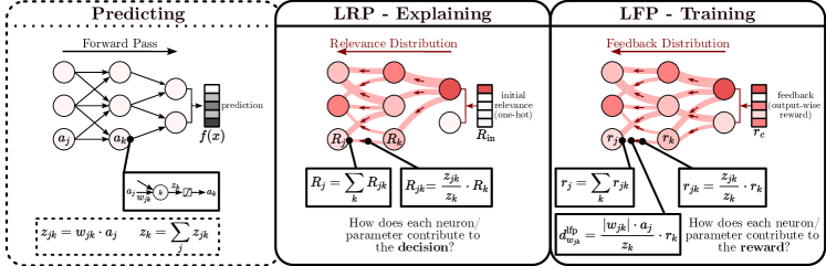
Figure 1: From LRP to LFP. [Left] The model makes a prediction during the forward pass. [Middle] LRP explains a specific decision by decomposing an initial relevance value and assigning credit to each neuron and connection, w.r.t. how (much) they contributed to this decision.[Right] LFP makes two adaptations to leverage this information for training: (I) Instead of an initial relevance value, a feedback is given to each output neuron evaluating how well it performed w.r.t. a given task. This feedback is then distributed to each latent neuron and parameter via LRP, assigning task-specific credit to each neuron and connection. (II) A parameter update $d^{\text{lfp}}_{w_{jk}}$ is derived from the credit assigned to connection $j\rightarrow k$.

In recent decades, gradient-based optimization techniques, as described by [1] have become the preferred method for optimizing complex machine learning (ML) models, including Deep Neural Networks (DNNs). This fundamental concept continues to drive groundbreaking advancements in AI, as the works of [2, 3, 4] demonstrate, among others. However, several issues have been identified with gradient-based training over the years. One such issue is the tendency for gradients to shatter in very deep models, resulting in behavior similar to white noise and making the training of deep models increasingly challenging [5]. Additionally, the utility of gradients for training is limited to scenarios where they are not undefined and at least provide meaningful information rather than returning zero or infinite values, which render optimization impossible. Although this leaves a broad range of functions, there are still important cases where direct application of gradients is impractical. For example, models that employ discrete activation functions (such as step functions), e.g., SNNs [6, 7].

Regarding training behavior, gradient-based optimization aims to identify the direction in the parameter space that results in the most significant reduction of the loss function. However, when dealing with large parameter spaces and complex loss landscapes, this approach can lead to unstable training behavior and high sensitivity to hyperparameters such as the learning rate. At the same time, previous research [8, 9] has demonstrated that even randomly initialized models with sufficient capacity often contain subnets that — when trained in isolation — are capable of achieving satisfactory performance on a given task. This suggests that deep models tend to be highly overparameterized in general. Given this observation, updating all parameters without discrimination towards a local optimum appears inefficient and unnecessarily unstable. It may be more advantageous to focus on identifying and extracting well-parameterized subnets that can be further optimized with minimal adjustments.

Due to the aforementioned limitations of gradient-based optimization, several alternative training methods have recently emerged. For instance, a number of studies [10, 11, 12, 13, 14] formulate neural network training as alternating minimization problems. Another set of approaches [15, 16, 17] involves training models through evolutionary strategies, by making random alterations to the model’s parameters and selecting the best-performing version. [18] propose modeling each synapse as a reinforcement learning agent using Q-learning, with a discrete action space consisting of increase, decrease, or no action. Another novel approach, introduced by [19], is the Forward-Forward Method, which employs a contrastive approach where the traditional backward pass is replaced with a second forward pass that operates on (generated) negative data. Each layer’s objective is to maximize the goodness on positive data while minimizing it on negative data. These alternative methods offer new perspectives and techniques for training neural networks, addressing the limitations of gradient-based optimization and exploring different optimization paradigms.

In recent years, the field of explainability has gained significant importance in the realm of AI. Within this field, a subset of methods [20, 21, 22, 23, 24] focuses on obtaining local explanations, which assign importance scores to individual features or groups of features in specific samples, based on the model’s behavior. These attribution scores provide insights into how the model responds to different features, offering a concise representation of its behavior. It is important to note that these methods are not limited to attributing importance solely to input features but can also determine the significance of individual units within a model. Previous studies have demonstrated the meaningfulness of these importance assignments, particularly in the case of LRP [23]. LRP has been successfully applied to a variety of tasks, including pruning [25] or quantizing [26] models, or to mitigate catastrophic forgetting [27].

LRP is a method that — after inference — is able to compute the contribution of network components to the prediction outcome. It achieves this by decomposing an initial relevance value at the output layer through a modified backward pass. Building upon this concept, we propose a novel approach called Layer-wise Feedback Propagation (LFP), which leverages LRP to distribute a reward (or feedback) to individual connections during training, based on an initial evaluation of the current prediction that measures its “goodness”. Through LFP, this feedback is distributed to each neuron and connection, assigning credit and providing a basis for updating parameters (see Figure 1). Fundamentally, while gradient-based optimization shifts all parameters towards the estimated direction of the largest decrease in loss, LFP distributes a reward to parameters, updating them based on their current contribution to solving the given task, thus implicitly working on a contributing subnet, relating it to the lottery ticket hypothesis [8, 9]. Rewards have shown great potential and have even been discussed as potential solutions for general AI [28], since they offer increased flexibility compared to the specificity of loss functions, potentially expanding the range of problems to which LFP can be applied.

Since LFP is a novel training paradigm, our primary objective is to demonstrate that it provides a valid training signal and converges to a local optimum. However, complex learning problems often require careful hyperparameter tuning and additional techniques for optimizing convergence, which have been extensively researched for gradient descent, the established method for training neural networks. For LFP, such optimizations do not yet exist and further research is needed to refine and improve its performance. Nevertheless, gradient descent serves as our baseline, and we compare it to LFP in our experiments by restricting evaluations to simpler toy settings. If LFP performs well in toy settings, this is likely to extend to more complex scenarios as well, with appropriate parameterization and further research. It is important to note that we do not advocate for or against favoring one method over the other. Rather, our focus lies in examining the similarities and differences between LFP and gradient descent — as both are backpropagation-based methods — as well as exploring potential applications for LFP. The current work serves as a foundation for understanding the fundamental aspects of LFP, with future investigations expected to address optimization challenges and explore its applicability in more complex scenarios.

To this end, we make the following contributions:

• We propose LFP, a novel paradigm for gradient-free training of DNNs.

• We demonstrate the performance of LFP theoretically via a convergence proof, as well as empirically on several different models and datasets.

• We investigate properties and potential applications of LFP beyond gradient-based training. Specifically, we look into the application of LFP to step-function-activated SNNs and of LFP as an efficient (in the sense of relevant parameters) transfer learning method.

To restrict the scope of this work, we select the well understood task of classification, using DNN models with one output neuron per class and no Batchnorm [29] layers. This fits well to our choice of feedback function (cf. Section 2.2) and to the implicit assumption of LRP with 0 as a reference value that is inherited by LFP as well. While more general formulations of LRP exist [30], exploring these for LFP is beyond the scope of this paper.

2 Layer-wise Feedback Propagation

2.1 Credit Assignment & Parameter Update

Let $x$ be a singular input sample to model $f$, with corresponding one-hot encoded ground-truth label $y\in\mathbb{R}^{C}$, and $C$ possible classes. Then, $f(x)$ denotes the model’s prediction on $x$, $o_{c}$ the logit of the output neuron corresponding to class $c$, and $a_{j}$ the output of an arbitrary neuron $j$. This output is computed as

$$a_{j}=\phi_{j}\left(\sum_{i}w_{ij}\cdot a_{i}\right)~{},$$ (1)

where $\phi_{j}$ denotes the activation function of neuron $j$ and the parameters $w_{ij}$ weigh the output $a_{i}$ of the $i$-th neuron. $w_{ij}$ may be 0 if there is no connection between $i$ and $j$. We view the bias $b_{j}$ of each neuron $j$ as weighted connections receiving $a_{b_{j}}=1$ in this context. As common in LRP-literature [31], we denote the contribution of a connection between neurons $i,j$ as $z_{ij}=w_{ij}\cdot a_{i}$ and the pre-activation of the $j$-th neuron as $z_{j}=\sum_{i}z_{ij}$.

LFP then assumes that a feedback $r_{c}$ is given to each output neuron $c$, assigning credit w.r.t. how well it contributes to solving the task. In other words, if a positive logit receives positive or negative feedback, it should increase or decrease, respectively. With the same-signed feedback, a negative logit should decrease or increase, respectively. Refer to Section 2.2 for more details. This feedback is then propagated backwards through the model based on LRP-rules, so that the $j$-th neuron eventually receives a feedback $r_{j}$. Here, the LRP-0-rule is used for simplicity, for LFP variants corresponding to other common LRP-rules and -composites, refer to Section 2.5. Then, the connection from $i$ to $j$ (i.e., weight $w_{ij}$) receives feedback $r_{ij}$ as

$$r_{ij}=\frac{z_{ij}}{z_{j}}\cdot r_{j}~{},$$ (2)

The feedback for neuron $i$ then accumulates as

$$r_{i}=\sum_{j}r_{ij}~{}.$$ (3)

Equation (3) inherently assigns credit to $a_{i}$, as Equation (2) does for $w_{ij}$, providing a notion of how helpful a parameter is in solving the task correctly.

In order to derive an update for $w_{ij}$, we replace $w_{ij}$ in $z_{ij}$ from Equation (2) with $\text{sign}(w_{ij})\cdot w_{ij}=|w_{ij}|$. I.e., we multiply feedback $r_{ij}$ with the parameter sign (since identically signed feedback should result in opposite update directions for negative/positive parameters) and thus arrive at the following update step:

$$d^{\text{lfp}}_{w_{ij}} =\frac{|w_{ij}|\cdot a_{i}}{z_{j}}\cdot r_{j}$$ (4)

$$w_{ij}^{\text{new}} =w_{ij}+\eta\cdot d^{\text{lfp}}_{w_{ij}}$$

Here, $\eta$ is a learning rate. We refer to this basic formulation of LFP as LFP-0. For instance, optimization akin to Stochastic Gradient Descent (SGD) with a momentum can then be described as follows:

$$d^{\text{momentum}}_{w_{ij}} =d^{\text{old}}_{w_{ij}}$$ (5)

$$d_{w_{ij}} =\alpha\cdot d^{\text{momentum}}_{w_{ij}}+(1-\alpha)\cdot d^{\text{lfp}}_{w_{ij}}$$

$$w_{ij}^{\text{new}} =w_{ij}+\eta\cdot d_{w_{ij}}$$

where $\alpha\in[0,1]$.

As a criterion, LFP employs a feedback instead of a loss function — requiring maximization instead of minimization in the update step of the above formula — guiding the model towards an optimum. This feedback is then distributed throughout the model in the update step, requiring no differentiation (Note: Equation (2) can be written as activation times gradient only for linear or ReLU-models. Consider e.g. the Heaviside step function which has zero or infinite gradients everywhere, but Equations (2) and (3) can still propagate a meaningful nonzero signal through models with Heaviside activations). Finally, we update model parameters based on the distributed feedback.

2.2 Feedback Functions

The feedback function is responsible for determining the initial feedback at the model output, and is subsequently decomposed throughout the model in order to assign credit w.r.t. the task to neurons and parameters.A positive feedback encourages the corresponding output, while a negative feedback discourages it. In that respect, it is similar to a reward function as used, e.g., in reinforcement learning.

However, while distributing a reward via the formulas proposed in Section 2.1 can yield meaningful update directions (cf. A.1), training will not converge: Since we derive updates directly from the credit assigned to connections via LFP (cf. Equation (4)), the updates will grow larger when greater rewards are earned due to improving performance, due to LRP conserving relevance across layers [23].

In order for training to converge, there are various options, such as early stopping, decaying learning rates, or decaying feedback, among others. As the convergence mechanism may be included in the reward function, affecting the received reward, we denote it as ”feedback” instead. In this paper, we choose the latter convergence mechanism, where the feedback must grow closer to zero, the larger the received reward becomes.

Let $\sigma(a)=\frac{1}{1+e^{-a}}$ be the sigmoid function.

During our experiments, we chose the following feedback function as it converged well in the investigated classification settings:

$$r(o_{c})=\begin{cases}o_{c}\cdot(1-\sigma(o_{c}))&\text{if }y_{c}=1\\ -o_{c}\cdot\sigma(o_{c})&\text{if }y_{c}=0\end{cases}$$ (6)

While the first factor of the multiplication (i.e., the logit $o_{c}$ or its negative $-o_{c}$) on its own is sufficient to produce a meaningful update, adding the factor on the right ensures that training also converges, by decaying feedback towards zero for logits with large magnitudes. Equation (6) can the be summarized as

$$r(o_{c})=o_{c}\cdot(y_{c}-\sigma(o_{c}))\text{.}$$ (7)

Note that the factor $(y_{c}-\sigma(o_{c}))$ is equivalent to the negative derivative of a binary crossentropy with a sigmoid, which allows for deriving a relationship to gradient descent in Section 2.3. Other feedback functions may perform similarly well or better. For instance, we show how a simple reward of -1 or 1 can be used for LFP in a simple toy setting in  A.1. However, as the choice of feedback function is not the main focus of this paper, we leave further investigation of it to later research.

2.3 Proof-of-Concept

In this Section, we show theoretically and experimentally that LFP converges, and is able to successfully train ML models. First, we show the following theorem:

Theorem 1.

For the feedback function employed in this paper (cf. Equation 7) and ReLU-activated models with non-negative logits, LFP-0 converges to a local minimum.

For the detailed proof refer to Appendix A.2. The proof relies on relating LFP to gradient descent as expressed by the chainrule, showing that the updates computed by LFP have the same sign as the updates computed via gradient descent. From there, convergence results for SignSGD [32] can be used.

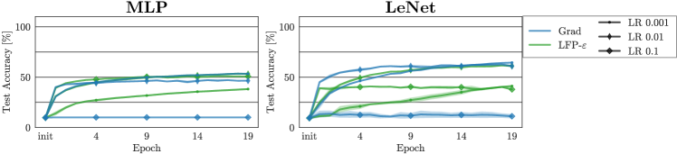
Figure 2: Performance of LFP-$\varepsilon$ vs. gradient backpropagation on the Cifar10 dataset. The experiment was performed using an MLP [left] and a LeNet [right], as well as three different learning rates (LR). LFP can achieve similar performance as gradient backpropagation, depending on hyperparameters such as the choice of learning rate or model. Both methods seem to require a different choice of hyperparameters for optimal performance. Results are averaged over 5 random seeds.

In a first experiment, we show that LFP is able to train models, achieving similar performances as gradient backpropagation, in a simple classification setting. For this purpose, we train a small MLP and a LeNet [33] model on the Cifar10 [34] dataset using both LFP-$\varepsilon$ (Equation 8) and gradient backpropagation. For more details about the specific setup refer to Appendix A.6.1.

Figure 2 shows the Cifar10-Training with LFP-$\varepsilon$ and gradient descent using different learning rates. While the learning rates at which both methods perform best differ, with the right choice of hyperparameters, LFP can achieve comparable performance gradient descent.

2.4 Relation to Gradient Descent

As shown in Section 2.3, LFP-0 as formulated in Equation (4) has the same sign as gradient descent in ReLU models, but may differ in the magnitude of updates. This does not hold for non-ReLU models or for different LFP-rules (see Section 2.5), where the updates caused by LFP and gradient descent may differ more significantly.

Fundamentally, LFP distributes a feedback signal to each connection and then derives an update for each connection depending on how it contributed. It improves useful connections and changes or diminishes obstructive ones. The advantage here is that LFP rewards/punishes how the model currently operates with potentially less disruptive updates (see e.g. the experiments in Sections 2.5 and 3), however, this also means that connections that do not contribute at all will not be updated. In contrast, gradient descent finds the direction in parameter space that minimizes a given loss function in estimation, generally updating all connections, no matter their contribution. Note also that LFP does not consider activation functions explicitly, only implicitly through the incoming feedback. LFP assumes that the model can be expressed in terms of layer-wise mappings $z_{ij}$ — which is the case, e.g., for neural networks, but it does not require the model to have meaningful derivatives (i.e., non-infinity and non-zero) and can therefore be applied to a different (although overlapping) set of problems than gradient descent (see e.g. Section 3).

2.5 LFP-Rules

The LFP-0-rule described in Section 2.1 captures the fundamental idea behind LFP, however, it is difficult to use in practice (comparable to the LRP-0-rule [23]), due to several undesirable properties: For instance, it becomes numerically unstable for denominators close to zero, and tends to cause backpropagated feedback to explode (although this is not exclusive to LFP, i.e., gradients can also explode) in deeper models if $|z_{ij}|\gg|z_{j}|$ (cf. Equation 3), which easily occurs when a neuron has both positive and negative contributions $z_{ij}$.

To resolve these problems, we extend LFP by three rules in the following, similar to what is done to render LRP numerically stable or adapt it to specific types of layers [23, 31]. For a detailed description of each rule and its potential benefits, please refer to Appendix A.3:

LFP-$\boldsymbol{\varepsilon}$ For this rule, a normalizing constant $\varepsilon$ is introduced for numerical stability, similar to LRP-$\varepsilon$ [23]:

$$r_{ij}=\frac{z_{ij}}{z_{j}+\text{sign}(z_{j})\cdot\varepsilon}\cdot r_{j}~{}$$ (8)

$$d^{\text{lfp}}_{w_{ij}}=\frac{|w_{ij}|\cdot a_{i}}{z_{j}+\text{sign}(z_{j})\cdot\varepsilon}\cdot r_{j}\\$$ (9)

LFP-$\boldsymbol{\alpha\beta}$ Treating positive and negative contributions separately can alleviate the issue of exploding feedback. With $z_{j}^{+}=\sum_{i}\text{max}(z_{ij},0)$ and $z_{j}^{-}=\sum_{i}\text{min}(z_{ij},0)$, we can formulate an LFP-$\alpha\beta$-rule as

$$r_{ij}=\begin{cases}\alpha\frac{z_{ij}}{z_{j}^{+}}\cdot\text{sign}(z_{j})\cdot r_{j}&\text{if }z_{ij}\geq 0\\ -\beta\frac{z_{ij}}{z_{j}^{-}}\cdot\text{sign}(z_{j})\cdot r_{j}&\text{else}{}\end{cases}$$ (10)

$$d^{\text{lfp}}_{w_{ij}}=\begin{cases}\alpha\frac{|w_{ij}|\cdot a_{i}}{z_{j}^{+}}\cdot\text{sign}(z_{j})\cdot r_{j}&\text{if }w_{ij}a_{i}\geq 0\\ -\beta\frac{|w_{ij}|\cdot a_{i}}{z_{j}^{-}}\cdot\text{sign}(z_{j})\cdot r_{j}&\text{else}{}\end{cases}~{},$$ (11)

subject to $\alpha-\beta=1$ to ensure the sum of feedback being conserved across layers in estimation.

We will investigate the behavior of LFP-$\alpha\beta$ in more detail in the experimental part of this section. In practice we use $\alpha=2$ and $\beta=1$ (called LFP-$\alpha 2\beta 1$ in the following), as this is a recommendation prevalent in LRP-literature [23], with the caveat that the values that work well for LRP may not carry over to LFP in the same manner. However, in-depth exploration of this parameter choice is beyond the scope of this paper.

LFP-$\boldsymbol{z^{+}z^{-}}$ In order to avoid exploding feedback and to adapt the general idea of the $\alpha\beta$-rule to updating parameters instead of explaining models, we further propose the LFP-$z^{+}z^{-}$-rule, which also treats positive and negative contributions separately, but relaxes the $\alpha-\beta=1$ constraint:

$$r_{ij}=\begin{cases}\frac{|z_{j}^{+}|}{|z_{j}^{+}|+|z_{j}^{-}|}\frac{z_{ij}}{z_{j}^{+}}\cdot\text{sign}(z_{j})\cdot r_{j}&\text{if }z_{ij}\geq 0\\ -\frac{|z_{j}^{-}|}{|z_{j}^{+}|+|z_{j}^{-}|}\frac{z_{ij}}{z_{j}^{-}}\cdot\text{sign}(z_{j})\cdot r_{j}&\text{else}{}\end{cases}$$ (12)

$$d^{\text{lfp}}_{w_{ij}}=\frac{|w_{ij}|\cdot a_{i}}{|z_{j}^{-}|+|z_{j}^{+}|}\cdot\text{sign}(z_{j})\cdot r_{j},$$ (13)

where the above formula is derived from Equation (A.13).

In practice, the stabilizing constant $\varepsilon$ from the previous paragraph is also applied to LFP-$\alpha\beta$ and LFP-$z^{+}z^{-}$ for numerical stability, but left out from the equations for readability.

All of the above rules can be applied in a layer-wise fashion and combined into composites [35], meaning that different rules are applied to different layers or types of layers. A description of the composites utilized in the following experiments can be found in Appendix A.6.2.

Effects of LFP-Rules After establishing that LFP is able to achieve comparable performances to gradient backpropagation in Section 2.3, we will now examine the effects of the different LFP-Rules introduced above, as well as gradient descent as a baseline. In a slighly more complex setting than for the previous experiments, we compare the different methods on a VGG-16 [36] model learning to classify a 20-class subset of the ImageNet [37] dataset. Both random initialization and pretraining on the original (1000-class) ImageNet dataset are utilized, with the latter aiming at evaluation of each method’s ability to retain and utilize existing information. More details on the training setup can be found in Appendix A.6.2.

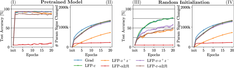
Figure 3: Performance and count of changing parameter signs on a 20-class ImageNet subset using VGG-16. Compared are both models pretrained on the original (1000-class) ImageNet [left], as well as trained from scratch [right]. Both test accuracy [I, III] and number of parameters that changed signs compared to the previous epoch [II, IV] are visualized. Gradient changes parameter signs (and thus their meaning) most significantly. While LFP-$\varepsilon$ performs similar to gradient descent, specifically LFP-$z^{+}z^{-}$ seems to perform much better on the pretrained model than on the randomly initialized one, while changing parameter signs only minimally.

Figure 3 shows the results of that experiment. Considering the randomly initialized setting first (III), we find that LFP-$\varepsilon$ is on par with gradient backpropagation in terms of performance, confirming the results of the previous section. However, all other composites perform significantly worse, with the mixed ones that employ LFP-$\varepsilon$ for dense layers leading to better accuracies than LFP-$z^{+}z^{-}$, and LFP-$\alpha 2\beta 1$ only achieving random performance. In the pretrained setting (I), only LFP-$\alpha 2\beta 1$ performs significantly lower than the other composites. The reason for this may be that while LFP-$\alpha 2\beta 1$ imposes a bound on the exploding feedback, it also introduces an average increase (assuming equal distribution of positively and negatively contributing connections) in feedback magnitude of 1.5 with each layer. For deep models, this may impact training more than for any other rules. Figure A.6 confirms through the MSE-difference between parameters at consecutive epochs that LFP-$\alpha 2\beta 1$ on average indeed leads to the largest updates by magnitude, supporting above interpretation. These results showcase that while LFP utilizes the basic formulation of LRP to measure parameter and neuron contribution, when it comes to specific rules and parameter choices, some adaptations need to be made, due to the diverging goals of explaining vs. learning between the two methods.

Comparing the number of changing parameter signs between methods, we observe that gradient backpropagation seems to change them most significantly, followed by LFP-$\varepsilon$ and the combined composites using LFP-$\varepsilon$. LFP-$\alpha 2\beta 1$ changes parameters the least. In fact, for the randomly initialized setting (IV), changing parameter signs more significantly seems to lead to better performance overall, which is consistent with the fact that the random model is not adapted to the classification task at all yet. However, in the finetuning setting (II), where the internal representations are already well-adapted to the task from initialization, composites that make less changes to parameter signs (excluding LFP-$\alpha 2\beta 1$ which behaves unstably assumedly due to exploding feedback) perform just as well as the gradient baseline. This observation is most significant for LFP-$z^{+}z^{-}$. As the sign of a parameter can be interpreted as the qualitative meaning of the corresponding connection (i.e., inhibitory or excitatory), not changing parameter signs during learning is interesting, as it implies a task-solving subnet being extracted and only finetuned in terms of quantitative contributions, not qualitative meaning, i.e., more existing knowledge is utilized, similar to what the lottery ticket hypothesis [8, 9] proposes. We will further investigate the LFP-$z^{+}z^{-}$ rule in that context in Section 3.2.

3 Applications

Despite certain similarities (cf. Sections 2.3, 2.4) to gradient descent, LFP functions differently, as it does not require gradients, propagates a reward, and bases its updates on the current contribution of connections. As such, it may have some advantages over gradient descent in specific settings (as well as disadvantages, as discussed in Section 2.4). To showcase some of these advantages, we will consider two specific applications in the following. Since LFP is a novel training method, we restrict experiments to simple problems and models, as application to more complex settings may require additional steps and optimizations that are subject to future work.

3.1 Application 1: Spiking Neural Networks

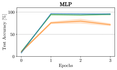
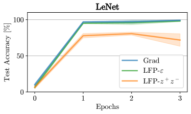
Figure 4: Test accuracy during the training process of the different examined methods on SNNs. Results depict the optimal performance achieved for each training method as determined via grid search hyperparameter optimization. The specific optimal hyperparameters used for each training approach are provided in Appendix A.6.3 (Table 1).

Spiking neural networks (SNNs) incorporate spiking neurons that resemble biological neural processing of information more closely compared to traditional artificial neural networks (ANNs) [6, 7]. However, the non-differentiable activation function of spike neurons poses a challenge for the application of gradient-based learning approaches that require differentiable operations. Thus, differentiable surrogate functions that approximate activation must typically be used during backpropagation to enable training [38]. When implementing such models directly in hardware, such an approximation could be extremely inefficient, as the (binary) step function would need to be replaced by a continuous function [39]. LFP provides a suitable training paradigm for SNNs that circumvents this limitation by propagating rewards directly through the non-differentiable spiking activation.

To evaluate our novel training method for SNNs, we utilized the LFP-$\varepsilon$ and LFP-$z^{+}z^{-}$ rules to train LeNet and fully-connected networks on the MNIST dataset [33]. Both networks employ Leaky Integrate-and-Fire (LIF) units, described by Equations (A.14)-(A.15). As a baseline, we used SGD training with a surrogate for the LIF unit to enable gradient computations. See Appendix A.6.3 for details on the experimental setup and the LIF units.

In Figure 4, the performance of the investigated training method is presented, with each technique utilizing its own set of optimal hyperparameters. The LFP training utilizing the LFP-$\varepsilon$ rule matches the accuracy obtained by gradient-based training without requiring any surrogate. In contrast, models trained with LFP-$z^{+}z^{-}$ do not achieve comparable results. This validates our findings at the end of Section 2.5.

During hyperparameter optimization, we found that LFP-based training exhibited greater performance variability compared to the baseline when exposed to different sequence lengths and membrane potential decay factors $\beta$ (cf. Figure A.4 in the Appendix). LFP generally performs better in the SNN setting when the membrane potential decays more slowly (at larger $\beta$ values) and with longer input sequences. This appears to stem from the sparsity induced by spiking neurons. A smaller $\beta$ implies a higher activation threshold for each neuron to spike and thus leads to network outputs that tend to be comprised mostly of zeros. With inactive neurons not transmitting information or contributing to the update, only few model updates can occur under these sparse conditions. We discuss this phenomenon in more detail in Section 2.4. Moreover, we empirically validated the impact of sparsity, see the Figure A.5. In contrast, longer sequences allow finer temporal encoding and more temporal relationships between neurons, benefiting training.

3.2 Application 2: LFP for Efficient Fine-tuning

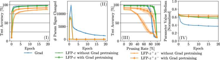
Figure 5: Performance (I). Parameter Sign Changes (II). Pruning LeNet models (lr 0.01) (III), using weight magnitude as a pruning criterion. Combinations of LFP and gradient descent are able to preserve accuracy for longer under pruning. LFP-$\varepsilon$ performs best in this sense. Parameter median (IV), normalized by the 75th percentile at each epoch. Averaged over 5 random seeds.

Since LFP updates the model based on the already present knowledge, its updates are less disruptive compared to those of gradient descent, as we already observed in the experiments of Section 2.5, where most LFP-composites (and LFP-$z^{+}z^{-}$ in particular) already changed parameter signs significantly less than gradient descent, while achieving comparable performances on a finetuning task. This is an interesting property, as it seems to confirm — since performance is matched while parameter signs barely change — that while LFP encourages any connections that contribute positively to solving the task, it tends to update obstructive connections towards zero rather than changing their sign, effectively pruning them (similar to an implicit LASSO-regularization [40]).

We compare the performance of gradient backpropagation, the LFP-$z^{+}z^{-}$-rule, and the LFP-$\varepsilon$-rule on MNIST using a LeNet model. For the LFP-rules, we investigate two variations each, one that uses gradient pretraining and then employs LFP for the remaining epochs, and one that completely trains the model using LFP, as shown in Figure 5.

From this Figure, we can make several observations. Firstly, LFP-$\varepsilon$ achieves final performances equal to gradient descent regardless of pretraining (I). LFP-$z^{+}z^{-}$ performs slightly worse, but achieves slightly better performance in the pretrained setting. Of the evaluated training methods, gradient descent converges the fastest — which extends to the LFP settings with gradient pretraing in comparison to their non-pretrained counterparts. However, when using gradient backpropagation, parameter signs change throughout the whole training process (although less the more training progresses), while they are constant as soon as LFP is applied (II).

We further investigate how well parameter magnitude aligns to its importance for predicting correctly (III): The value of a parameter is not always a good indicator for how significant the corresponding connection is to making correct predictions [25]. However, if obstructive connections are updated towards zero instead of changing signs, while beneficial connections increase in magnitude, parameter value should correlate significantly more to parameter importance. To evaluate this, we employ a simple pruning setup based on the weight magnitude (i.e., the weights with the smallest absolute value are pruned first similar to [41]). Here, the models trained with LFP-$\varepsilon$ are able to preserve their performance the longest, until almost 90% of weights are pruned. In contrast, models trained with gradient backpropagation lose performance around 70% weights pruned. For LFP-$z^{+}z^{-}$, we observe a significant effect of the pretraining, with the setting employing pretraining being able to preserve performance for much longer than without (the same effect can be observed for LFP-$\varepsilon$ as well, but far less significant). Despite the performance of LFP-$z^{+}z^{-}$ starting to decrease as early as 20-40% under pruning, especially for the pretrained setting, it decreases comparatively slowly, and even overtakes gradient descent above 80% parameters pruned.

We interpret this result as follows: LFP is mainly able to utilize and extract the knowledge already present in the model (coinciding with observations in the experiments in Section 2.5). Here, LFP-$\varepsilon$ seems to be more accurate in its updates, achieving better performances. In contrast, gradient backpropagation can optimize parameters regardless of knowledge already existing within the model. However, after a good configuration has been found, it exhibits high volatility in parameter space, changing more than necessary. So, when instead employing the modified LFP after gradient pretraining, LFP starts from a good “initialization”, and is able to utilize existing knowledge well. Especially LFP-$z^{+}z^{-}$ benefits from this pretraining. We can observe (IV) that gradient descent significantly reduces the median parameter magnitude especially in the beginning of training, indicating a higher number of comparatively large parameters. Between LFP-$z^{+}z^{-}$ and LFP-$\varepsilon$, the former seems to change distribution of parameter magnitudes the least across training, explaining why it is far more sensitive to the initialization. We initially introduced the LFP-$z^{+}z^{-}$-rule in order to mitigate exploding feedback occurring for the base formulation as well as LFP-$\varepsilon$. LFP-$\varepsilon$ vastly outperformed LFP-$z^{+}z^{-}$ in this experiment. However, as exploding feedback only becomes an issue with deep models, and the model employed here is quite shallow, we suspect LFP-$z^{+}z^{-}$ may perform significantly better in more complex transfer-learning settings (cf. Figure 3).

4 Conclusion

In this work we introduced LFP, a novel XAI-based paradigm for training neural networks that backpropagates a feedback in order to update parameters with out requiring computation of gradients.

We found that with the right choice of hyperparameters, LFP is able to arrive at similarly accurate solutions as gradient descent on several different models and datasets. We further extended several LRP-rules to LFP, providing solutions for the issues of numerical stability and exploding feedback that the base formulation of LFP suffers from. With LFP being a gradient-free method, it is able to train models with derivatives that make application of gradient descent impossible, e.g., SNNs, however, we also found that performance in this setting largely depends on hyperparameters due to LFP being unable to propagate feedback through inactive neurons. In a second application, we investigated the utility of LFP as a transfer learning method, and found that while performance of LFP is on par with gradient descent, it barely changes parameter signs during training, decaying obstructive connections towards zero, effectively pruning them. The resulting model demonstrated a far better relationship between parameter magnitude and ablative parameter importance to model performance than models trained fully via gradient descent, however, as already observed in the SNN application, LFP often has difficulties training randomly initialized models from scratch, as it utilizes existing knowledge to improve the model.

As this paper mainly served as an introduction of LFP and demonstration of its potential applications, in-depth investigation of the effects of hyperparameters such as $\alpha,\beta$ in the $\alpha\beta$-rule, learning rate, or feedback function, among others, are subject to future work. Similarly, our experiments were performed in relatively simple settings, and extensions to state-of-the-art problems will be explored in follow-up works. However, since LFP mainly builds upon knowledge already present in a model, it may be best suited for transfer learning, or applications where meaningful derivatives cannot be computed. With the main idea behind LFP being the distribution of a reward via LRP, possible extensions include disconnecting the credit assignment and derived updates, in order to avoid the update magnitude for a connection being determined by its reward magnitude.

Appendix A Appendix

A.1 LFP with Simplistic Rewards

While we observed the feedback function from Equation (7) to converge well in the investigated settings, LFP can also backpropagate other feedback functions, such as standard rewards. To shortly demonstrate this, we train a small ReLU-activated fully-connected model (32, 32, 2 neurons) on 2-class one-dimensional toy data (from $-4$ to $4$ in steps of $5\cdot 10^{-4}$, with the sign denoting the class assignment and 100 random samples being held out for testing). The backpropagated signal is normalized by its maximum absolute value after passing through each layer. SGD with a learning rate of 1.0 and a momentum of 0.9 is employed for optimization. As feedback, only the true-class output neuron receives a reward; 1 for a correct classification and -1 for a wrong classification. LFP-$\varepsilon$ is used for training. As shown in Figure A.1, this yields a meaningful signal for updating weights as well, however, it quickly becomes unstable if some manner of convergence is not ensured. In Equation (7), this is done through the sigmoid term, however, other methods would be applicable as well, e.g., early stopping or the learning rate scheduling employed here (learning rate is multiplied with 0.1 every 40 steps).

Figure A.1: LFP-$\varepsilon$ with a simple reward-function. This does yield meaningful update signals, however, convergence still needs to be ensured in some way (here through a diminishing learning rate), otherwise training can become unstable.

A.2 Proof of Theorem 1

Proof.

We prove the convergence of LFP by relating it to gradient descent with a binary crossentropy loss. Specifically, we show that — provided the restrictions of the proven theorem (Feedback function from Equation 7, ReLU-activated models, LFP-0, and logits $o_{c}\geq 0$) — the updates computed by LFP have under a condition shown below the same sign as the updates computed via gradient descent.

As the sign is the driving factor behind convergence [42], the key to prove convergence lies in showing that the signs of gradient descent and LFP are matching.

This principle, namely, that the sign is the relevant component for an effective update when minimizing a loss under small step sizes, is known in the adversarial attack community, where it is exploited in the mechanisms of the Fast Gradient Sign Method adversarial attack (FGSM) [43] and iterative FGSM attacks [44, 45, 46]. The convergence of SignSGD and SigNum in theory has been established under mild conditions in Section 3 of [32].

The gradient used to update weights can be expressed by chainrule into three terms:

$$\frac{\partial L}{\partial w_{ij}}=\sum_{c}{\underbrace{\vphantom{\frac{\partial a_{j}}{\partial w_{ij}}}\frac{\partial L}{\partial o_{c}}}_{\textbf{I}}}\cdot{\underbrace{\vphantom{\frac{\partial a_{j}}{\partial w_{ij}}}\frac{\partial o_{c}}{\partial a_{j}}}_{\textbf{II}}}\cdot{\underbrace{\frac{\partial a_{j}}{\partial w_{ij}}}_{\textbf{III}}}$$ (A.1)

where $\frac{\partial L}{\partial o_{c}}$ is the partial derivative of the loss with respect to the logit $o_{c}$ and $\frac{\partial o_{c}}{\partial a_{j}}$ is the partial derivative of the logit $o_{c}$ with respect to the neuron $a_{j}$ to which the parameter $w_{ij}$ belongs to. When considering the gradient in equation (A.1) together with the LFP-update $d^{\text{lfp}}_{w_{ij}}$ from Equation (4), as well as Equations (2) and (3)), we can observe an analogous structure:

$$d^{\text{lfp}}_{w_{ij}}=\sum_{c}r(o_{c})\cdot r(o_{c}\rightarrow a_{j})\cdot r(a_{j}\rightarrow w_{ij})~{},$$ (A.2)

where $r(o_{c})$ denotes the feedback received by the logit $o_{c}$, $r(o_{c}\rightarrow a_{j})$ the feedback flowing from $o_{c}$ to activation $a_{j}$ and $r(a_{j}\rightarrow w_{ij})$ the feedback flowing from $a_{j}$ to $w_{ij}$ for the update step. In the following, $\text{sign}(\cdot)$ denotes the sign-function.

(I)

Firstly, the feedback function in Equation (7) contains the derivative of a binary crossentropy (BCE) with a sigmoid, with a negative sign:

BCE Derivative: $$\frac{\partial L}{\partial o_{c}} =\sigma(o_{c})-y_{c}$$ (A.3)

Feedback Eq (7): $$r(o_{c}) =o_{c}\cdot(y_{c}-\sigma(o_{c}))$$ (A.4)

$o_{c}$ in Equation (7) is a simple scaling factor. Consequently, and since $o_{c}\geq 0$ the following holds:

$$\operatorname{\text{sign}}(r(o_{c}))=-\operatorname{\text{sign}}(\frac{\partial L}{\partial o_{c}})$$ (A.5)

The sign is different, which makes sense because the weight update employs the negative gradient, whereas for LFP-Feedback we do not switch signs.

(II)

Instead of the middle term $\frac{\partial o_{c}}{\partial a_{j}}$, LFP utilizes the feedback $r(o_{c}\rightarrow a_{j}))$ sent from logit $o_{c}$ to neuron $a_{j}$ to compute neuron feedback $r_{j}$, as described by Equations 2 and 3. As LFP employs LRP to backpropagate feedback, this is equal to computing the LRP-relevance $R(o_{c}\rightarrow a_{j})$ of $a_{j}$ with respect to output $o_{c}$ (cf. Equations 2, 3 and LRP-Equations, e.g., from [23]).

We can show that this term is correlated to the partial derivative II from Equation (A.1). Let $z$ denote the current value of $a_{j}$. The important property is that relevance explains the prediction relative to a zero state. If $R(o_{c}\rightarrow a_{j})$ is positive, it implies that setting $a_{j}$ to zero would decrease $o_{c}$. Then, using Taylor approximation

$$R(o_{c}\rightarrow a_{j})>0 \Rightarrow o_{c}\mid_{a_{j}=z}>o_{c}\mid_{a_{j}=0}$$ (A.6)

$$\Rightarrow 0<o_{c}\mid_{a_{j}=z}-o_{c}\mid_{a_{j}=0}$$

$$\approx\frac{\partial o_{c}}{\partial a_{j}}(z)(z-0)$$

Analogously, if $R(o_{c}\rightarrow a_{j})$ of $a_{j}$ is negative, then it implies that setting $a_{j}$ to zero would increase $o_{c}$:

$$R(o_{c}\rightarrow a_{j})<0 \Rightarrow o_{c}\mid_{a_{j}=z}<o_{c}\mid_{a_{j}=0}$$ (A.7)

$$\Rightarrow 0>o_{c}\mid_{a_{j}=z}-o_{c}\mid_{a_{j}=0}$$

$$\approx\frac{\partial o_{c}}{\partial a_{j}}(z)(z-0)$$

For ReLU units we have always $z\geq 0$. Therefore, whenever the approximation of the difference $o_{c}\mid_{a_{j}=z}-o_{c}\mid_{a_{j}=0}$ by the partial derivative $\frac{\partial o_{c}}{\partial a_{j}}(z)$ times the value $z$ holds, the relevance $R(o_{c}\rightarrow a_{j})$ has the same sign as the partial derivative $\frac{\partial o_{c}}{\partial a_{j}}(z)$ . Thus, for ReLU-models, we can expect to have

$$\operatorname{\text{sign}}(R(o_{c}\rightarrow a_{j})) =\operatorname{\text{sign}}(\frac{\partial o_{c}}{\partial a_{j}})$$ (A.8)

The approximation might not hold for $|z|$ sufficiently large. The experiments show that the impact of possible violations are limited.

(III)

Lastly, for the third term $\frac{\partial a_{j}}{\partial w_{ij}}$, we show that it has for ReLU activations the same sign as LFP from Equation (4). Let $z_{j}$ denote the pre-activation corresponding to $a_{k}$. Here, we consider two cases:

1. In the first case, if the output of $a_{j}$ is zero: $a_{j}=0\geq z_{j}$, then it receives in the backward pass also zero feedback $r_{j}$ via LFP (cf. Equations 2, 3):

$$r_{j} =\sum_{k}r_{jk}$$ (A.9)

$$=\sum_{k}\frac{w_{jk}\cdot a_{j}}{z_{k}}\cdot r_{k} |a_{j}=0$$

$$=0=\frac{\partial a_{j}}{\partial w_{ij}}~{},$$

which means that the weight update $d^{\text{lfp}}_{w_{ij}}$ from Equation (4) also becomes zero. 2. In the second case, if the ReLU value is positive, i.e. $z_{j}=a_{j}>0$, then

$$a_{j}=z_{j} =\sum_{i}w_{ij}a_{i}\geq 0\text{ and }$$ (A.10)

$$\frac{\partial a_{j}}{\partial w_{ij}} =a_{i}~{},$$

and we can rewrite the distribution of feedback to the weight update in Equation (4) (denoted as $r(a_{j}\rightarrow w_{ij})$) as follows:

$$r(a_{j}\rightarrow w_{ij}) =\frac{|w_{ij}|\cdot a_{i}}{z_{j}}$$ (A.11)

$$=a_{i}\cdot\frac{|w_{ij}|}{z_{j}}$$

$$=\frac{\partial a_{j}}{\partial w_{ij}}\cdot\frac{|w_{ij}|}{z_{j}} |z_{j}>0$$

$$\propto\frac{\partial a_{j}}{\partial w_{ij}}$$

Putting (I), (II), and (III) and Equation (A.2) together, we get:

$$\operatorname{\text{sign}}(d^{\text{lfp}}_{w_{ij}}) =\begin{cases}\operatorname{\text{sign}}(\frac{\partial a_{j}}{\partial w_{ij}}))&\text{if }a_{j}=0\\ \begin{gathered}\parbox[t]{108.405pt}{$\operatorname{\text{sign}}(r(o_{c}))\cdot\operatorname{\text{sign}}(r(o_{c}\rightarrow a_{j}))\\ \cdot\operatorname{\text{sign}}(r(a_{j}\rightarrow w_{ij}))$}\end{gathered}&\text{else.}\end{cases}$$ (A.12)

$$\approx\begin{cases}\operatorname{\text{sign}}(\frac{\partial a_{j}}{\partial w_{ij}}))|=0&\text{if }a_{j}=0\\ \begin{gathered}\parbox[t]{108.405pt}{$-\operatorname{\text{sign}}(\frac{\partial L}{\partial o_{c}})\cdot\operatorname{\text{sign}}(\frac{\partial o_{c}}{\partial a_{j}})\\ \cdot\operatorname{\text{sign}}(\frac{\partial a_{j}}{\partial w_{ij}})$}\end{gathered}&\text{else.}\end{cases}$$

$$=-\operatorname{\text{sign}}(\frac{\partial L}{\partial o_{c}})\cdot\operatorname{\text{sign}}(\frac{\partial o_{c}}{\partial a_{j}})\cdot\operatorname{\text{sign}}(\frac{\partial a_{j}}{\partial w_{ij}})$$

$$=-\operatorname{\text{sign}}(\frac{\partial L}{\partial w_{ij}})$$

Consequently, all three terms from Equation (A.1) can be related to a corresponding counterpart from LFP. The sign of $d^{\text{lfp}}_{w_{ij}}$ from Equation (4) opposes the sign of $\frac{\partial L}{\partial w_{ij}}$. This, however, leads to the same update direction for $w_{ij}$ as LFP adds the update with a positive sign (Equation (4)), while the gradient decent update step contains a negative sign.

∎

A.3 Details of LFP-Rules

LFP-$\boldsymbol{\varepsilon}$ This rule introduces a normalizing constant $\varepsilon$ to the denominator for numerical stability. However, similar to the LFP-0-rule presented in Section 2.1, this rule can still lead to exploding feedback when applied in succession across layers, although this does not necessarily seem to be the case in practice (see Figure 3). We use $\varepsilon=10^{-6}$ in our experiments.

LFP-$\boldsymbol{\alpha\beta}$ By separating positive and negative contributions, LFP-$\alpha\beta$ is able to bound the explosion of feedback in the backward pass. It is inspired by LRP, where several rules, e.g., the LRP-$\alpha\beta$-rule [23], treat positive and negative contributions separately, as this aligns well to the behavior of layers that output only positive values, e.g., ReLU-activated layers. Note that both $0\leq\frac{z_{ij}}{z_{j}^{+}}\leq 1$ and $0\leq\frac{z_{ij}}{z_{j}^{-}}\leq 1$ hold. Thus, LFP-$\alpha\beta$ alleviates exploding feedback by introducing an upper bound of $\text{max}(|\alpha|,|\beta|)$ to the magnitude of the factor by which feedback can potentially explode with each additional layer. Note also the multiplication with $\text{sign}(z_{j})$ in Equations (10), (11), different to LRP-$\alpha\beta$, this is due to the feedback $r_{j}$ rewarding the actual output $z_{j}$ and its sign, and not the partial contributions $z_{j}^{+},~{}z_{j}^{-}$.

LFP-$\alpha\beta$ thus may not fully solve the issue of exploding feedback, depending on the choice of $\alpha$ and $\beta$. Exploding feedback can only be avoided for both $\alpha,\beta\in[0,1]$ which — under the constraint $\alpha-\beta=1$ — is only given for $\alpha=1,\beta=0$, in which case obstructive connections would not receive any updates. While this relevance-conserving method of separating positive and negative contributions is useful when explaining layers with specific activation functions [23], this does not necessarily make sense for training, e.g., if this leads to positively contributing connections being updated more than negatively contributing ones.

LFP-$\boldsymbol{z^{+}z^{-}}$ extends the general idea of the LFP-$\alpha\beta$ to single neurons, separating positive and negative contributions, but making exploding feedback impossible. The factors $\alpha,\beta$ are replaced by adaptive factors $\frac{|z_{j}^{+}|}{|z_{j}^{+}|+|z_{j}^{-}|}\in[0,1]$ and $\frac{|z_{j}^{-}|}{|z_{j}^{+}|+|z_{j}^{-}|}\in[0,1]$, that sum to 1 and make exploding feedback impossible. As such, LFP-$z^{+}z^{-}$ can be viewed as a special case of LFP-$\alpha\beta$ with parameters that vary for each neuron. While it does not conserve the sum of feedback across layers (as LFP-$\alpha\beta$ aims to do), it imposes a bound on feedback magnitude

The unshortened formulation of the LFP-$z^{+}z^{-}$-rule is as follows:

$$d^{\text{lfp}}_{w_{ij}}=\begin{cases}\frac{|z_{j}^{+}|}{|z_{j}^{-}|+|z_{j}^{+}|}\frac{|w_{ij}|\cdot a_{i}}{z_{j}^{+}}\cdot\text{sign}(z_{j})\cdot r_{j}&\text{if }w_{ij}a_{i}\geq 0\\ -\frac{|z_{j}^{-}|}{|z_{j}^{-}|+|z_{j}^{+}|}\frac{|w_{ij}|\cdot a_{i}}{z_{j}^{-}}\cdot\text{sign}(z_{j})\cdot r_{j}&\text{else}{}\end{cases}$$ (A.13)

A.4 Shattering Behavior of Gradients vs. LFP

Using the same dataset as in Section A.1, but sampled with a stepsize of 0.02 instead, similar to the one employed by [5], we further investigate the shattering behavior of gradients and different LFP-Rules. The employed model consists of a variable number of ReLU-activated dense layers, with 200 neurons at the first layer, 2 neurons at the output layer, and a variable number of 200-neuron hidden layers in between. The backpropagated signal is normalized by its maximum absolute value after passing through each layer. We plot the backpropagated signal at the input for LFP and gradients.

As shown in Figure A.2 — corroborating the results from [5] —, gradients become increasingly noise-like for deeper models. I.e., the correlation between gradient values for similar inputs decreases with depth. A similar behavior can be observed for LFP-$\varepsilon$, which not only becomes uncorrelated to the input, but seems to vanish as well. In contrast, the LFP rules that distinguish between positive and negative contributions seem to not shatter to the same extent. Especially LFP-$z^{+}z^{-}$ seems to provide an extremely stable signal even for 500 hidden layers.

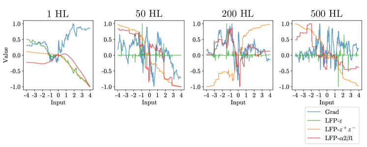
Figure A.2: Gradient and LFP values at the input for models with increasing depth. With increasing depth (number of hidden layers (HL)), both gradients and LFP-$\varepsilon$ seem to approach noise processes, with barely any correlation between values at neighboring inputs. In contrast, LFP-$\alpha 2\beta 1$ and especially LFP-$z^{+}z^{-}$ seem to have similar values for similar inputs.

We further investigate to what extend this property may make LFP more robust against network depth. For this purpose, we train a ReLU-activated fully-connected model on the same dataset as in A.1. The model consists of a varying number of hidden layers (1–20) and an output layer with two neurons. We repeat the experiment with varying numbers of neurons per layer (repeated for values 8, 16, 32, and 64). SGD with a learning rate of 1.0 and a momentum of 0.9 is employed for optimization, and the model is trained for 5 epochs on the dataset from above. The backpropagated signal is normalized by its maximum absolute value after passing through each layer. Results are shown in Figure A.3 averaged over 3 random seeds and the different values of neurons per layer.

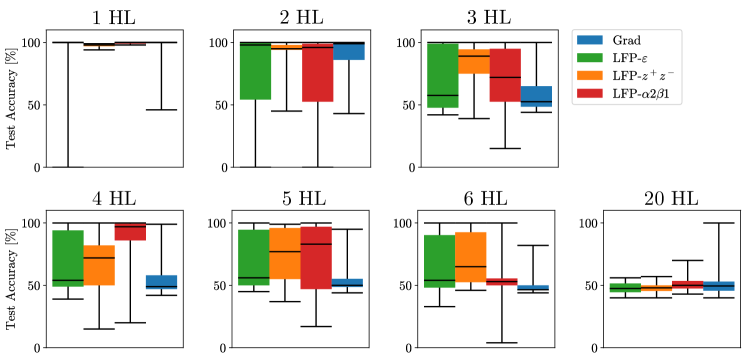
Figure A.3: Accuracies for training models with an increasing number of hidden layers (HL). Each bar shows, from bottom to top, the following values, measured over 12 runs each (three different seeds and four different values for neurons per hidden layer): minimum, 25th percentile, median, 75th percentile, maximum. LFP-$z^{+}z^{-}$ and LFP-$\alpha 2\beta 1$ seem to be most robust against depth. Despite that, performance is already significantly reduced at 6HL, and completely random at 20HL

Figure A.3 shows the results of that experiment. In correspondence to the results observed in Figure A.2, LFP-$z^{+}z^{-}$ and LFP-$\alpha 2\beta 1$ seem to be most robust against depth, up to a certain degree. However, even at six hidden layers, their performance is severely impacted, and at 20 hidden layers, it is completely random. As shattering is not the only issue with training deep models (e.g., internal covariate shift [29] occurs in parallel), we can only expect a limited effect of reducing shattering. Nevertheless, we can observe a clear trend in favor of LFP-$z^{+}z^{-}$ and LFP-$\alpha 2\beta 1$, but this effect would need to be studied more thoroughly in future work.

A.5 Spiking Neural Networks

Spiking neural networks (SNNs) [6, 7] are a special type of recurrent network build out of spiking neurons that model biological processing in real brains more closely than conventional neurons in ANNs. Spiking neurons have a membrane potential $U\in\mathbb{R}$ that dictates whether a neuron sends out a discrete spike or remains inactive. The output of neurons in a SNN can be modeled using the Heaviside step function:

$$\operatorname*{H}\left(U[t]-\theta\right)=\begin{cases}1&\text{if}~{}U[t]>\theta\\ 0&\text{else}\end{cases}$$ (A.14)

where

$$U[t]\coloneqq\beta U[t-1]+WX[t]-\theta\operatorname{H}\left(U[t-1]-\theta\right).$$ (A.15)

Here, the hyperparameter $\beta\in(0,1]$ controls the decay of the membrane potential and $\theta\in\mathbb{R}$ is a threshold that determines the membrane potential required for the neuron to fire. The learnable parameters associated with the input connections originating from the output $X[t]$ of the preceding layer are denoted as $W$. The final summand in Equation (A.15) resets the membrane potential after the neuron has fired. For more details see [6] and [38].

Implemented on neuromorphic hardware, SNNs exhibit advantageous features such as energy-efficient inference, event-based processing, and the ability to learn online [39].

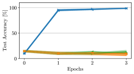
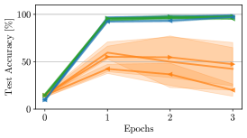
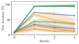
(a) LeNet

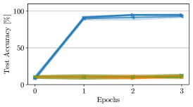
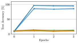
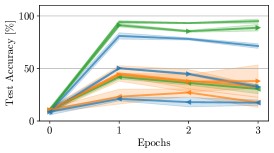
(b) MLP

Figure A.4: Performance comparison of spiking neural networks (SNNs) with LeNet [top] and MLP [bottom] architecture trained using different learning rules. A fixed learning rate of $LR{=}10^{-3}$ and varying sequence lengths ($L$) and potential decay factors ($\beta$) were utilized. In the left, middle and right columns, $\beta$ was set to $0.3,0.6$ and $0.9$ respectively. Training with LFPs demonstrated diminished performance for small $\beta$ compared to gradient-based training. This is hypothesized to result from the sparsity induced by spiking neurons, which limits the contribution of most network components and prevents effective updating by LFP, as discussed in Section 2.4. Results are averaged across three random seeds.

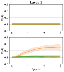
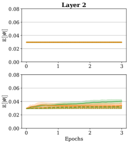
(a) Mean of the absolute values of the bias parameters during training. Top row: $\beta=0.3$. Bottom row: $\beta=0.6$.

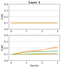
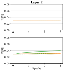
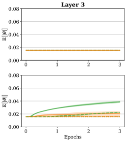
(b) Mean of the absolute values of the weight parameters during training. Top row: $\beta=0.3$. Bottom row: $\beta=0.6$.

Figure A.5: Mean magnitude changes of parameters during LFP-training for varying learning rates ($LR$), potential decay factors ($\beta$), and a fixed sequence length $L=5$ using the LeNet architecture. With $\beta=0.3$, most parameters underwent only negligible updates, except for bias terms in the final layer. However, with $\beta=0.6$, the increased information flow enabled larger, more evenly distributed parameter updates across layers. Similar results were obtained using MLP architectures. Results are averaged across three random seeds.

A.6 Details on Experiments

Of the experiments in this work, the ones in Appendix A.1 and A.4, as well as the pruning and parameter median computation in Application 2 (Figure 5 (III) and (IV)) were computed on a local machine, while all other experiments were run on an HPC Cluster.

The local machine used Ubuntu 20.04.6 LTS, an NVIDIA TITAN RTX Graphics Card with 24GB of memory, an Intel Xeon CPU E5-2687W V4 with 3.00GHz, and 32GB of RAM.

The HPC-Cluster used Ubuntu 18.04.6 LTS, an NVIDIA A100 Graphics Card with 40GB of memory, an Intel Xeon Gold 6150 CPU with 2.70GHz, and 512GB of RAM. Apptainer was used to containerize experiments on the cluster.

All experiments were implemented in python, using PyTorch [47] for deep learning, including weights available from torchvision, as well as snnTorch [38] for SNN applications. matplotlib was used for plotting. The implementation of LFP builds upon zennit [48], an XAI-library.

A.6.1 Proof-of-Concept

Both an MLP and a LeNet [33] were trained for 20 epochs on the Cifar10 benchmark dataset [34] with a batch size of 32. The MLP consists of four dense layers with 512, 256, 128, and 10 neurons, respectively, and three dropout layers ($p=0.5$) in between. The LeNet has two convolutional layers with 16 channels and a kernel-size of 5 each, followed by three dense layers (120, 84, 10 neurons) with dropout layers ($p=0.5$) in between. Models are ReLU-activated and were trained using either gradient backpropagation or LFP-$\varepsilon$. SGD with a momentum of $0.9$ and learning rates $10^{-1}$, $10^{-2}$, and $10^{-3}$ was utilized for optimization of both training paradigms. Categorical crossentropy was utilized as the criterion for gradient descent. The experiment was repeated 5 times for each setting with different random seeds, and results averaged.

A.6.2 Effects of LFP-Rules

A VGG-16 model [36] was trained for 20 epochs on a 20-class subset of the ImageNet (ILSVRC2012) Dataset [37] (classes "Mailbox", "Maillot", "Medicine Chest", "Mobile Home", "Notebook", "Sea Snake", "Bouvier des Flandres", "American Alligator", "Walker Hound", "Dishwasher", "Street Sign", "Tub", "Coho", "Ear", "Great Pyrenees", "Ground Beetle", "Rule", "Megalith", "Three-toed Sloth", "Dhole") with a batch size of 32. Models were trained using both gradient backpropagation, and various LFP-composites: LFP-$\varepsilon$, LFP-$z^{+}z^{-}$, and LFP-$\alpha 2\beta 1$ apply the respective rule to all layers. LFP-$\varepsilon$-$z^{+}z^{-}$ and LFP-$\varepsilon$-$\alpha 2\beta 1$ apply LFP-$\varepsilon$ to the dense layers of the classifier, and LFP-$z^{+}z^{-}$ or LFP-$\alpha 2\beta 1$ to the convolutional layers in the feature extractor, respectively. For the pretrained model, ImageNet weights available from the torchvision framework were utilized. We employed Adam with an initial learning rate of $10^{-4}$ for optimization, and a categorical crossentropy criterion for gradient backpropagation. The experiment was repeated 3 times for each setting with different random seeds; results are averaged over these.

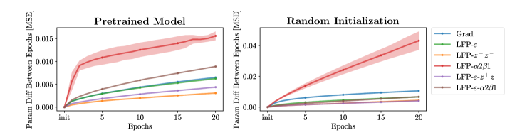
Figure A.6: MSE between parameters at consecutive epochs for different LFP-rules (cf. Figure 3). The LFP-$\alpha 2\beta 1$-rule leads to the largest parameter updates, LFP-$z^{+}z^{-}$ to the smallest parameter updates on average

A.6.3 Application 1: Spiking Neural Networks

For this study, LeNet and multilayer perceptron (MLP) architectures were trained on the MNIST dataset [33] for image classification. The LeNet architecture consisted of two successive convolution blocks followed by a final MLP block. The convolution blocks each contained a convolution layer with 12 and 64 channels, respectively, utilizing $5{\times}5$ kernels with stride 1 and no input padding. Max pooling layers with $2{\times}2$ kernels and stride 2 followed, along with the leaky integrate-and-fire (LIF) activation functions (refer to Equations (A.14)-(A.15)). The final MLP classification block contained a dense layer of 1,024 LIF neurons followed by a final application of the LIF non-linearity.
The MLP architecture consisted of three dense layers each followed by the LIF non-linearity. The dimension of the hidden layers was set to 1,000.
For the LIFs activation function we adapted the implementation from [38]. To enable gradient-based training we utilized the surrogate function $s\colon\mathbb{R}\to\mathbb{R}$ with $x\mapsto{x}\cdot({1+25\cdot\lvert x\rvert})^{-1}$ in the backward pass during the related experiments.
Experiments were conducted with a fixed LIF threshold of $\theta{=}1$ and varying the decay factor $\beta$ to values of $0.3$, $0.6$, and $0.9$. The sequence length $L$ was varied across $5$, $15$, and $25$ time steps. Both networks were trained for three epochs using a batch size of $128$. For optimization, the Adam algorithm was utilized with beta parameters of $0.9$ and $0.999$. Learning rates of $10^{-3}$, $10^{-4}$, and $10^{-5}$ were investigated. For stability, the backward pass was normalized by the maximum absolute value between layers. Additionally we utilized the adaptive gradient clipping strategy proposed in [49]. The experiments were performed across three different random seeds, with results averaged.
For the gradient-based training, the categorical cross-entropy loss was employed between the one-hot encoded target classes and the accumulated per-output spike counts.
The LFP training methodology requires a reward function. For these experiments, the reward described in Equation (6) was adapted as follows to enable sequence-based inputs and outputs:

For the SNNs experiments, the static MNIST images are encoded into the required input sequence through constant encoding. Specifically, a given image $X_{i}\in\mathbb{R}^{w\times h\times c}$ is fed continuously into the network $n$ times, yielding the input $X{\in}\mathbb{R}^{n\times w\times h\times c}$. When presented with the input $X$, the SNNs produces an output sequence $(o_{c,i})_{i=1}^{n}$ per class, with $1\leqslant c\leqslant m$ denoting the class. This can be written as an output matrix $O\in\mathbb{R}^{n,m}$ where the rows correspond to the individual output sequences. Given the corresponding target label $y_{c}\in\mathbb{N}$ the reward matrix $R\in\mathbb{R}^{n,m}$ is element wise defined via

$$r_{c,i}{=}\begin{cases}\textstyle~{}{+1}\big{(}{1{-}\sigma(\sum_{i}o_{c,i}-\tfrac{n}{2})}\big{)}&\text{if}~{}y_{c}{=}c\\ \textstyle{-o_{c,i}}\big{(}1{-}\sigma(\sum_{i}(o_{c,i}{-}1){-}\tfrac{n}{2})\big{)}&\text{if}~{}y_{c}{\neq}c.\end{cases}$$ (A.16)

	LR $M^{M^{M}}$	$\beta$	$L$
LFP-$\varepsilon$	$10^{-3}$ $M^{M^{M}}$	$0.9$	$25$
LFP-$z^{+}z^{-}$	$10^{-4}$	$0.9$	$25$
Grad	$10^{-3}$	$0.6$	$25$

Table 1: Optimized hyperparameter values for each training methodology utilized during the SNNs experiments (refer to Figure 4).

A.6.4 Application 2: LFP for Efficient Fine-tuning

The same LeNet model as described in A.6.1 was trained for 10 epochs with batch size 32 on the MNIST benchmark dataset. Gradient backpropagation and the LFP-$z^{+}z^{-}$ and LFP-$\varepsilon$-rules were used as training paradigms, in addition to a combined approach where gradient backpropagation was used for the first 100 iterations and the modified LFP for the rest. Optimization was performed using SGD with a momentum of 0.9 and a learning rate of $10^{-2}$. For stability, the backward pass was normalized by the maximum absolute value between layers. For gradient backpropagation, a categorical crossentropy criterion was employed. Results are averaged over 5 random seeds.

References

- [1] D. E. Rumelhart, G. E. Hinton, and R. J. Williams, “Learning internal representations by error propagation,” California Univ San Diego La Jolla Inst for Cognitive Science, Tech. Rep., 1985.
- [2] Q. V. Le, “Building high-level features using large scale unsupervised learning,” in IEEE International Conference on Acoustics, Speech and Signal Processing, ICASSP 2013, Vancouver, BC, Canada, May 26-31, 2013. IEEE, 2013, pp. 8595–8598.
- [3] K. He, X. Zhang, S. Ren, and J. Sun, “Deep residual learning for image recognition,” in 2016 IEEE Conference on Computer Vision and Pattern Recognition, CVPR 2016, Las Vegas, NV, USA, June 27-30, 2016. IEEE Computer Society, 2016, pp. 770–778.
- [4] K. Han, A. Xiao, E. Wu, J. Guo, C. Xu, and Y. Wang, “Transformer in transformer,” in Advances in Neural Information Processing Systems 34: Annual Conference on Neural Information Processing Systems 2021, NeurIPS 2021, December 6-14, 2021, virtual, M. Ranzato, A. Beygelzimer, Y. N. Dauphin, P. Liang, and J. W. Vaughan, Eds., 2021, pp. 15 908–15 919.
- [5] D. Balduzzi, M. Frean, L. Leary, J. P. Lewis, K. W.-D. Ma, and B. McWilliams, “The shattered gradients problem: If resnets are the answer, then what is the question?” in Proceedings of the 34th International Conference on Machine Learning, ser. Proceedings of Machine Learning Research, vol. 70. PMLR, 06–11 Aug 2017, pp. 342–350.
- [6] W. Maass, “Networks of spiking neurons: The third generation of neural network models,” Neural Networks, vol. 10, no. 9, pp. 1659–1671, Dec. 1997.
- [7] F. Ponulak and A. Kasinski, “Introduction to spiking neural networks: Information processing, learning and applications,” Acta Neurobiologiae Experimentalis, vol. 71, no. 4, pp. 409–433, 2011.
- [8] J. Frankle and M. Carbin, “The lottery ticket hypothesis: Finding sparse, trainable neural networks,” in 7th International Conference on Learning Representations, ICLR 2019, New Orleans, LA, USA, May 6-9, 2019. OpenReview.net, 2019.
- [9] E. Malach, G. Yehudai, S. Shalev-Shwartz, and O. Shamir, “Proving the lottery ticket hypothesis: Pruning is all you need,” in Proceedings of the 37th International Conference on Machine Learning, ICML 2020, 13-18 July 2020, Virtual Event, ser. Proceedings of Machine Learning Research, vol. 119. PMLR, 2020, pp. 6682–6691.
- [10] M. Á. Carreira-Perpiñán and W. Wang, “Distributed optimization of deeply nested systems,” in Proceedings of the Seventeenth International Conference on Artificial Intelligence and Statistics, AISTATS 2014, Reykjavik, Iceland, April 22-25, 2014, ser. JMLR Workshop and Conference Proceedings, vol. 33. JMLR.org, 2014, pp. 10–19.
- [11] G. Taylor, R. Burmeister, Z. Xu, B. Singh, A. B. Patel, and T. Goldstein, “Training neural networks without gradients: A scalable ADMM approach,” in Proceedings of the 33nd International Conference on Machine Learning, ICML 2016, New York City, NY, USA, June 19-24, 2016, ser. JMLR Workshop and Conference Proceedings, M. Balcan and K. Q. Weinberger, Eds., vol. 48. JMLR.org, 2016, pp. 2722–2731.
- [12] J. Wang, F. Yu, X. Chen, and L. Zhao, “ADMM for efficient deep learning with global convergence,” in Proceedings of the 25th ACM SIGKDD International Conference on Knowledge Discovery & Data Mining, KDD 2019, Anchorage, AK, USA, August 4-8, 2019, A. Teredesai, V. Kumar, Y. Li, R. Rosales, E. Terzi, and G. Karypis, Eds. ACM, 2019, pp. 111–119.
- [13] J. Zeng, T. T. Lau, S. Lin, and Y. Yao, “Global convergence of block coordinate descent in deep learning,” in Proceedings of the 36th International Conference on Machine Learning, ICML 2019, 9-15 June 2019, Long Beach, California, USA, ser. Proceedings of Machine Learning Research, K. Chaudhuri and R. Salakhutdinov, Eds., vol. 97. PMLR, 2019, pp. 7313–7323.
- [14] J. Wang, H. Li, and L. Zhao, “Accelerated gradient-free neural network training by multi-convex alternating optimization,” Neurocomputing, vol. 487, pp. 130–143, 2022.
- [15] T. Salimans, J. Ho, X. Chen, and I. Sutskever, “Evolution strategies as a scalable alternative to reinforcement learning,” CoRR, vol. abs/1703.03864, 2017.
- [16] F. P. Such, V. Madhavan, E. Conti, J. Lehman, K. O. Stanley, and J. Clune, “Deep neuroevolution: Genetic algorithms are a competitive alternative for training deep neural networks for reinforcement learning,” CoRR, vol. abs/1712.06567, 2017.
- [17] R. Tripathi and B. Singh, “RSO: A gradient free sampling based approach for training deep neural networks,” CoRR, vol. abs/2005.05955, 2020.
- [18] A. Bhargava, M. R. Rezaei, and M. Lankarany, “Gradient-free neural network training via synaptic-level reinforcement learning,” CoRR, vol. abs/2105.14383, 2021.
- [19] G. E. Hinton, “The forward-forward algorithm: Some preliminary investigations,” CoRR, vol. abs/2212.13345, 2022.
- [20] D. Baehrens, T. Schroeter, S. Harmeling, M. Kawanabe, K. Hansen, and K. Müller, “How to explain individual classification decisions,” Journal of Machine Learning Research, vol. 11, pp. 1803–1831, 2010.
- [21] K. Simonyan, A. Vedaldi, and A. Zisserman, “Deep inside convolutional networks: Visualising image classification models and saliency maps,” CoRR, vol. abs/1312.6034, 2013.
- [22] J. Springenberg, A. Dosovitskiy, T. Brox, and M. Riedmiller, “Striving for simplicity: The all convolutional net,” in ICLR (workshop track), 2015.
- [23] S. Bach, A. Binder, G. Montavon, F. Klauschen, K.-R. Müller, and W. Samek, “On pixel-wise explanations for non-linear classifier decisions by layer-wise relevance propagation,” PLoS ONE, vol. 10, no. 7, p. e0130140, 2015.
- [24] M. Sundararajan, A. Taly, and Q. Yan, “Axiomatic attribution for deep networks,” CoRR, vol. abs/1703.01365, 2017.
- [25] S. Yeom, P. Seegerer, S. Lapuschkin, A. Binder, S. Wiedemann, K. Müller, and W. Samek, “Pruning by explaining: A novel criterion for deep neural network pruning,” Pattern Recognit., vol. 115, p. 107899, 2021.
- [26] D. Becking, M. Dreyer, W. Samek, K. Müller, and S. Lapuschkin, “Ecq: Explainability-driven quantization for low-bit and sparse dnns,” in xxAI - Beyond Explainable AI - International Workshop, Held in Conjunction with ICML 2020, July 18, 2020, Vienna, Austria, Revised and Extended Papers, ser. Lecture Notes in Computer Science, A. Holzinger, R. Goebel, R. Fong, T. Moon, K. Müller, and W. Samek, Eds., vol. 13200. Springer, 2022, pp. 271–296.
- [27] S. Ede, S. Baghdadlian, L. Weber, A. Nguyen, D. Zanca, W. Samek, and S. Lapuschkin, “Explain to not forget: Defending against catastrophic forgetting with XAI,” in Machine Learning and Knowledge Extraction - 6th IFIP TC 5, TC 12, WG 8.4, WG 8.9, WG 12.9 International Cross-Domain Conference, CD-MAKE 2022, Vienna, Austria, August 23-26, 2022, Proceedings, ser. Lecture Notes in Computer Science, A. Holzinger, P. Kieseberg, A. M. Tjoa, and E. R. Weippl, Eds., vol. 13480. Springer, 2022, pp. 1–18.
- [28] D. Silver, S. Singh, D. Precup, and R. S. Sutton, “Reward is enough,” Artif. Intell., vol. 299, p. 103535, 2021.
- [29] S. Ioffe and C. Szegedy, “Batch normalization: Accelerating deep network training by reducing internal covariate shift,” in Proceedings of the 32nd International Conference on Machine Learning, ICML 2015, Lille, France, 6-11 July 2015, ser. JMLR Workshop and Conference Proceedings, F. R. Bach and D. M. Blei, Eds., vol. 37. JMLR.org, 2015, pp. 448–456.
- [30] S. Letzgus, P. Wagner, J. Lederer, W. Samek, K. Müller, and G. Montavon, “Toward explainable AI for regression models,” CoRR, vol. abs/2112.11407, 2021.
- [31] G. Montavon, A. Binder, S. Lapuschkin, W. Samek, and K. Müller, “Layer-wise relevance propagation: An overview,” in Explainable AI: Interpreting, Explaining and Visualizing Deep Learning, ser. Lecture Notes in Computer Science, W. Samek, G. Montavon, A. Vedaldi, L. K. Hansen, and K. Müller, Eds. Springer, 2019, vol. 11700, pp. 193–209.
- [32] J. Bernstein, Y. Wang, K. Azizzadenesheli, and A. Anandkumar, “SIGNSGD: compressed optimisation for non-convex problems,” in Proceedings of the 35th International Conference on Machine Learning, ICML 2018, Stockholmsmässan, Stockholm, Sweden, July 10-15, 2018, ser. Proceedings of Machine Learning Research, J. G. Dy and A. Krause, Eds., vol. 80. PMLR, 2018, pp. 559–568.
- [33] Y. LeCun, L. Bottou, Y. Bengio, and P. Haffner, “Gradient-based learning applied to document recognition,” Proc. IEEE, vol. 86, no. 11, pp. 2278–2324, 1998.
- [34] A. Krizhevsky, “Learning multiple layers of features from tiny images,” Master’s thesis, University of Toronto, Department of Computer Science, 2009.
- [35] M. Kohlbrenner, A. Bauer, S. Nakajima, A. Binder, W. Samek, and S. Lapuschkin, “Towards best practice in explaining neural network decisions with LRP,” in 2020 International Joint Conference on Neural Networks, IJCNN 2020, Glasgow, United Kingdom, July 19-24, 2020. IEEE, 2020, pp. 1–7.
- [36] K. Simonyan and A. Zisserman, “Very deep convolutional networks for large-scale image recognition,” CoRR, vol. abs/1409.1556, 2014.
- [37] A. Krizhevsky, I. Sutskever, and G. E. Hinton, “Imagennet classification with deep convolutional neural networks,” in Advances in Neural Information Processing Systems (NIPS), 2012, pp. 1097–1105.
- [38] J. K. Eshraghian, M. Ward, E. Neftci, X. Wang, G. Lenz, G. Dwivedi, M. Bennamoun, D. S. Jeong, and W. D. Lu, “Training spiking neural networks using lessons from deep learning,” CoRR, vol. abs/2109.12894, 2021.
- [39] M. Pfeiffer and T. Pfeil, “Deep Learning With Spiking Neurons: Opportunities and Challenges,” Frontiers in Neuroscience, vol. 12, 2018.
- [40] R. Tibshirani, “Regression shrinkage and selection via the lasso,” Journal of the Royal Statistical Society Series B: Statistical Methodology, vol. 58, no. 1, pp. 267–288, 1996.
- [41] S. Han, J. Pool, J. Tran, and W. J. Dally, “Learning both weights and connections for efficient neural network,” in Advances in Neural Information Processing Systems 28: Annual Conference on Neural Information Processing Systems 2015, December 7-12, 2015, Montreal, Quebec, Canada, C. Cortes, N. D. Lawrence, D. D. Lee, M. Sugiyama, and R. Garnett, Eds., 2015, pp. 1135–1143.
- [42] Q. Liao, J. Z. Leibo, and T. A. Poggio, “How important is weight symmetry in backpropagation?” in Proceedings of the Thirtieth AAAI Conference on Artificial Intelligence, February 12-17, 2016, Phoenix, Arizona, USA, D. Schuurmans and M. P. Wellman, Eds. AAAI Press, 2016, pp. 1837–1844.
- [43] I. J. Goodfellow, J. Shlens, and C. Szegedy, “Explaining and harnessing adversarial examples,” in 3rd International Conference on Learning Representations, ICLR 2015, San Diego, CA, USA, May 7-9, 2015, Conference Track Proceedings, Y. Bengio and Y. LeCun, Eds., 2015.
- [44] A. Kurakin, I. J. Goodfellow, and S. Bengio, “Adversarial machine learning at scale,” in International Conference on Learning Representations, 2017.
- [45] Y. Dong, F. Liao, T. Pang, H. Su, J. Zhu, X. Hu, and J. Li, “Boosting adversarial attacks with momentum,” in 2018 IEEE/CVF Conference on Computer Vision and Pattern Recognition, 2018, pp. 9185–9193.
- [46] C. Xie, Z. Zhang, Y. Zhou, S. Bai, J. Wang, Z. Ren, and A. L. Yuille, “Improving transferability of adversarial examples with input diversity,” in 2019 IEEE/CVF Conference on Computer Vision and Pattern Recognition (CVPR), 2019, pp. 2725–2734.
- [47] A. Paszke, S. Gross, F. Massa, A. Lerer, J. Bradbury, G. Chanan, T. Killeen, Z. Lin, N. Gimelshein, L. Antiga, A. Desmaison, A. Köpf, E. Yang, Z. DeVito, M. Raison, A. Tejani, S. Chilamkurthy, B. Steiner, L. Fang, J. Bai, and S. Chintala, “Pytorch: An imperative style, high-performance deep learning library,” in Advances in Neural Information Processing Systems (NeurIPS), 2019, pp. 8024–8035.
- [48] C. J. Anders, D. Neumann, W. Samek, K.-R. Müller, and S. Lapuschkin, “Software for dataset-wide xai: From local explanations to global insights with Zennit, CoRelAy, and ViRelAy,” CoRR, vol. abs/2106.13200, 2021.
- [49] A. Brock, S. De, S. L. Smith, and K. Simonyan, “High-performance large-scale image recognition without normalization,” in Proceedings of the 38th International Conference on Machine Learning, ICML 2021, 18-24 July 2021, Virtual Event, ser. Proceedings of Machine Learning Research, M. Meila and T. Zhang, Eds., vol. 139. PMLR, 2021, pp. 1059–1071.