Bias-Aware Minimisation: Understanding and
Mitigating Estimator Bias in Private SGD

Abstract

Differentially private SGD (DP-SGD) holds the promise of enabling the safe and responsible application of machine learning to sensitive datasets. However, DP-SGD only provides a biased, noisy estimate of a mini-batch gradient. This renders optimisation steps less effective and limits model utility as a result. With this work, we show a connection between per-sample gradient norms and the estimation bias of the private gradient oracle used in DP-SGD. Here, we propose Bias-Aware Minimisation (BAM) that allows for the provable reduction of private gradient estimator bias. We show how to efficiently compute quantities needed for BAM to scale to large neural networks and highlight similarities to closely related methods such as Sharpness-Aware Minimisation. Finally, we provide empirical evidence that BAM not only reduces bias but also substantially improves privacy-utility trade-offs on the CIFAR-10, CIFAR-100, and ImageNet-32 datasets.

1 Introduction

The application of machine learning models to datasets containing sensitive information necessitates meaningful privacy guarantees, as it has been shown that the public release of unsecured models trained on sensitive data can pose serious threats to data-contributing individuals [1, 2, 3]. To this end, differential privacy (DP) [4], the widely accepted gold standard approach to privacy-preserving data analysis, has been extended to many machine learning methods. Most significantly, for modern machine learning, differentially private stochastic gradient descent (DP-SGD) [5, 6] has enabled the application of powerful deep neural networks to sensitive datasets with meaningful privacy guarantees.

In practice, however, DP-SGD comes with a substantial utility penalty. As we demonstrate below, this is because DP-SGD only provides a noisy, biased gradient estimate, causing optimization to settle in regions of the loss landscape that yield poorly performing models. We show that (ignoring sampling noise), the variance of a private gradient estimate is fixed while its bias is not. In this work, we attempt to improve private gradient estimators by minimising their bias. The bias of an estimate $\hat{p}$ of the true value $p$ underlying a process generating observations $x$ is defined as:

$$\mathrm{Bias}(\hat{p},p)=\mathbb{E}_{x}[\hat{p}]-p.$$ (1)

Figure 1: (a) Clipping per-sample gradients $g_{1}$ and $g_{2}$ yields a biased gradient estimate $\boldsymbol{\hat{g}_{\mathrm{clip}}}$ of the true mini-batch gradient $\boldsymbol{\hat{g}}$ in expectation. Below we show this bias, represented by the vector $\boldsymbol{\text{Bias}(\hat{g}_{\text{priv}},\hat{g},)}$ in (b), to depend on $\lVert g_{1}\rVert_{2}$ and $\lVert g_{2}\rVert_{2}$.

Thus, when an estimator has zero bias, it is called unbiased and its expected value is equal to the quantity being estimated. When estimating gradients, unbiasedness is a useful property as it implies that gradient estimates –in expectation– point towards the correct descent direction.

Bias in DP-SGD results from the per-sample gradient clipping operation, used to enforce a sensitivity bound on the gradients (illustrated above in Fig. 1). However, despite its importance, the nature of this bias and how it affects parameter updates has remained poorly understood. With this work, we show that private gradient estimator bias is intimately related to the per-sample gradient norms and can further be decomposed into a magnitude and directional component (See Appendix C). We develop Bias-Aware Minimisation (BAM) and provide empirical evidence that our method effectively (I) reduces bias magnitude and (II) increases classification performance on a range of challenging vision benchmarks.

2 Related Work

The bias-variance tradeoff of the private gradient oracle was first discussed in [7]. More generally, bias associated with gradient clipping in SGD has been studied by Zhang et al. [8], Qian et al. [9] and also in the private setting, where Song et al. [10] demonstrated the importance of the correct choice of clipping threshold in convex models, while Chen et al. [11] showed that no bias is incurred when a symmetricity condition on the gradient distribution holds.

Concurrent work [12, 13] has provided empirical evidence that Sharpness-Aware-Minisation (SAM) [14] can improve privacy-utility tradeoffs. Park et al. [12] suggest that the magnitude of the bias vector (referred to as the effect of clipping in their work) is bounded by the sharpness. With this work, we provide evidence that sharpness, while closely related, might not be the root cause determining private gradient bias but rather the per-sample gradient norms in a mini-batch.

3 Preliminaries

Differential privacy [15] (DP), is a stability notion on randomised mechanisms over sensitive databases. Let $D$ and $D^{\prime}$ be two databases (datasets) that differ exactly in one individual’s data. We denote this relationship (i.e. database adjacency) through the symbol $\simeq$ and use the standard remove/add one relation throughout.

Definition 1 (Differential privacy).

A randomised mechanism $M$ executed on the result of a query function $q$ (i.e. $M(q(\cdot))$) preserves $(\varepsilon$, $\delta)$-DP if, for all pairs of adjacent databases $D$ and $D^{\prime}$, and all subsets $\mathcal{S}$ of $M(q(\cdot))$’s range:

$$p\left[M\left(q(D)\right)\in\mathcal{S}\right]\leq{e^{\varepsilon}}\,p\left[M(q(D^{\prime}))\in\mathcal{S}\right]+\delta,$$ (2)

where the relationship between $D$ and $D^{\prime}$ is symmetric. The guarantee is given over the randomness of $M$.

To achieve $(\varepsilon,\delta)$-DP using Gaussian noise perturbation (i.e. the Gaussian mechanism $\mathcal{M}$), one needs to calibrate the magnitude of the noise to the query function’s (global) sensitivity:

$$\Delta_{2}(q)=\sup_{D\simeq D^{\prime}}\left\lVert q(D)-q(D^{\prime})\right\rVert_{2},$$

or $\Delta$ for short. Since obtaining a (non-vacuous) sensitivity bound is generally not possible for deep neural network gradients, it is common practice to enforce a bound manually by projecting per-sample gradients to the $L_{2}$-ball [6]. Together, this operation, more commonly known as clipping, followed by appropriately scaled Gaussian perturbation, then yields the DP-SGD algorithm, which can be thought of as simply querying a private gradient oracle at each optimisation step as seen in Algorithm 1:

Algorithm 1 Private gradient oracle $\psi$

Input: (Poisson-sampled) mini-batch $B=\{(x_{1},y_{1}),...,(x_{l},y_{l})\}$, Clipping Bound $C$, noise multiplier $\sigma$, loss function $\mathcal{L}$, parameters $\theta\in\mathbb{R}^{d}$
Output; private gradient estimate

$(x_{i},y_{i})$in $B$

1:$g_{i}\leftarrow\nabla_{\theta}\mathcal{L}\left(f_{\theta}(x_{i}),y_{i}\right)$

2:$\bar{g}_{i}\leftarrow g_{i}/\max(1,\frac{\left\lVert g_{i}\right\rVert_{2}}{C})$ $\triangleright$ clip

3:$\hat{g}_{\mathrm{priv}}\leftarrow\frac{1}{l}\left(\sum_{i=1}^{l}\bar{g}_{i}+\mathcal{N}(0,\sigma^{2}C^{2}I_{d})\right)$ $\triangleright$ perturb

4:return $\hat{g}_{\mathrm{priv}}$

Where $l$ is the expected batch size due to the sub-sampling amplification requirement that $B$ is constructed through a Poisson sample of the Dataset $D$.

3.1 Setting

We focus on supervised learning where, given a dataset $D=\{(x_{i},y_{i}),...,(x_{n},y_{n})\}$ drawn i.i.d from a product distribution $\mathcal{X}\times\mathcal{Y}$, we wish to find a mapping $f:\mathcal{X}\rightarrow\mathcal{Y}$, realised through a neural network. This neural network has parameters $\theta\in\Theta\in\mathbb{R}^{d}$ and is trained by minimising the empirical loss function $\mathcal{L}(\theta):=\frac{1}{n}\sum_{i=1}^{n}\mathcal{L}(\theta,x_{i},y_{i})$ using DP-SGD, whereby at each optimisation step the private gradient oracle is queried to obtain a privatised gradient estimate.

$$\theta^{(t+1)}=\theta^{(t)}-\gamma^{(t)}\hat{g}^{(t)}_{\mathrm{priv}}$$ (3)

$$\hat{g}^{(t)}_{\mathrm{priv}}=\psi(B,C,\sigma,\mathcal{L},\theta^{t})$$ (4)

We drop the superscript $t$ for notational simplicity, assuming we are on step $t$ in the following analyses. We further denote the clipped minibatch gradient as $\hat{g}_{\mathrm{clip}}=1/l\sum_{i}^{l}\bar{g}_{i}$.

4 Clipping dominates private gradient bias

Since we are interested in obtaining an unbiased version of DP-SGD, we first study the bias introduced by constructing a private estimate for the mini-batch gradient $\hat{g}$. Our analysis focuses on the quantity:

$$\text{Bias}\left(\hat{g}_{\mathrm{priv}},\,\hat{g}\right)=\mathbb{E}[\hat{g}_{\mathrm{priv}}]-\hat{g},$$

where we view $\hat{g}$ as fixed, that is, the gradient constructed for an already observed batch of data to be used in a step of conventional SGD. This enables us to isolate the bias introduced through private estimation of $\hat{g}$. Note that when using $\mathbb{E}$ without a subscript, we take the expectation over all randomness present. In the case of $\hat{g}_{\mathrm{priv}}$, this randomness is –by assumption– only due to the Gaussian mechanism. We first observe that this gradient perturbation does not introduce additional bias:

Lemma 1.

The bias of the private gradient estimate, Bias($\hat{g}_{\mathrm{priv}},\hat{g})$, is unaffected by the noise addition in the Gaussian mechanism. That is,

$$\mathrm{Bias}(\hat{g}_{\mathrm{priv}},\hat{g})=\mathrm{Bias}(\hat{g}_{\mathrm{clip}},\hat{g})$$

Proof.

$$\mathrm{Bias}(\hat{g}_{\mathrm{priv}}, \hat{g})=\mathbb{E}\Big{[}\frac{1}{l}\sum_{i=1}^{l}\Big{(}\mathrm{clip}(g_{i})+\mathcal{N}(0,\sigma^{2}C^{2}I_{d})\Big{)}\Big{]}-\hat{g}$$ (5)

$$= \frac{1}{l}\sum_{i=1}^{l}\Big{(}\mathrm{clip}(g_{i})+\mathbb{E}\big{[}\mathcal{N}(0,\sigma^{2}C^{2}I_{d})\big{]}\Big{)}-\hat{g}$$ (6)

$$= \hat{g}_{\mathrm{clip}}-\hat{g}$$ (7)

$$= \mathrm{Bias}(\hat{g}_{\mathrm{clip}},\hat{g})$$ (8)

This holds since $\hat{g}$ and $\hat{g}_{\mathrm{clip}}$ are viewed as constructed from an observed mini-batch of data and the zero centred Gaussian random variables are independent of one another. ∎

Thus, private gradient bias is caused by the clipping operation alone. Next, we develop an objective function that provably minimises the aforementioned bias.

5 A bias-aware objective

We propose $\mathcal{L}_{\mathrm{BAO}}$, an objective that, when minimised, provably reduces the bias of private gradient estimates $\hat{g}_{\mathrm{priv}}$ by encouraging small per-sample gradient norms:

$$\mathcal{L}_{\mathrm{BAO}}(\theta,x,y)=\underbrace{\mathcal{L}(\theta,x,y)}_{\text{original loss}}+\underbrace{\lambda\left(\frac{1}{l}\sum_{i=1}^{l}\left\lVert g_{i}\right\rVert_{2}\right)}_{\text{regularising term}}$$ (9)

which can be sub-sampled as follows:

$$\mathcal{L}_{\mathrm{BAO}}(\theta,x_{i},y_{i})=\mathcal{L}(\theta,x_{i},y_{i})+\lambda\left\lVert g_{i}\right\rVert_{2}$$ (10)

To motivate this optimisation objective, we will now demonstrate the primary dependence of Bias($\hat{g}_{\mathrm{priv}},\hat{g})$ on the per-sample gradient norms for a fixed clipping threshold $C$.

Lemma 2.

A smaller per-sample gradient norm $\lVert g_{i}\rVert_{2}$ of the $i$-th sample in a mini-batch decreases $\text{Bias}(\hat{g}_{\mathrm{priv}},\hat{g})$.

Proof.

First note that

$$\mathrm{clip}(g_{i})=\frac{g_{i}}{\mathrm{max}(1,\frac{\lVert g_{i}\rVert_{2})}{C})}=\begin{cases}g_{i}&\mathrm{if}\,\lVert g_{i}\rVert_{2}\leq C\\ \frac{Cg_{i}}{\lVert g_{i}\rVert_{2}}&\mathrm{if}\,\lVert g_{i}\rVert_{2}>C.\end{cases}$$

Thus, if $\lVert g_{i}\rVert_{2}\leq C$ for every $i$ in the mini-batch, then by Lemma 1:

$$\mathrm{Bias}(\hat{g}_{\mathrm{priv}},\hat{g})=\frac{1}{l}\sum_{i=1}^{l}g_{i}-\hat{g}=0.$$

That is, if the $L_{2}$-norm of the gradients of the mini-batch are all below the clipping threshold, the bias of the private gradient estimate reduces to zero. On the other hand, if $\lVert g_{i}\rVert_{2}>C$:

$$\mathrm{Bias}(\hat{g}_{\mathrm{priv}},\hat{g}) =\frac{1}{l}\sum_{i=1}^{l}\frac{C}{\lVert g_{i}\rVert_{2}}g_{i}-\hat{g}.$$ (11)

Therefore, the bias is dependent on the ratios $\frac{C}{\lVert g_{i}\rVert_{2}}\forall i$: as a per-sample gradient norm $\lVert g_{i}\rVert_{2}$ gets increasingly larger than $C$, the bias grows (note that here grows means gets further from the origin). Conversely, if we minimise $\lVert g_{i}\rVert_{2}$ for any $i$, the bias will shrink until all $\left\lVert g_{i}\right\rVert_{2}$ in the mini-batch are less than $C$, at which point the estimate becomes unbiased. ∎

Notice that (9) is similar to the gradient norm penalty, used by [16] to encourage flatness of the loss landscape:

$$\mathcal{L}_{Z}(\theta)=\mathcal{L}(\theta)+\left\lVert\nabla_{\theta}\mathcal{L}(\theta)\right\rVert_{2},$$ (12)

It can be shown that (9) upper-bounds $\mathcal{L}_{Z}$ (see Appendix B). This means that a reduction in $\mathcal{L}_{\mathrm{BAO}}$ implies a reduction in $\mathcal{L}_{Z}$, but the converse is not generally true. Note also that $\mathcal{L}_{Z}$ does not allow for the required per-sample DP analysis, precluding the simple application of DP-SGD [12].

Dataset	$\boldsymbol{\varepsilon}$	$\boldsymbol{\delta}$	DP-SGD	DP-SAT	BAM (ours)
CIFAR-10	$1.0$	$10^{-5}$	$60.9\pm 0.49$	$60.9\pm 0.62$	$\mathbf{61.4\pm 0.48}$
	$2.0$		$67.1\pm 0.10$	$67.2\pm 0.30$	$\mathbf{68.2\pm 0.27}$
	$10.0$		$78.6\pm 0.08$	$78.1\pm 0.69$	$\mathbf{79.7\pm 0.13}$
CIFAR-100	$1.0$	$10^{-5}$	$18.1\pm 0.10$	$18.2\pm 0.13$	$\mathbf{18.5\pm 0.04}$
	$2.0$		$24.9\pm 0.46$	$24.9\pm 0.35$	$\mathbf{25.4\pm 0.40}$
	$10.0$		$40.3\pm 0.21$	$40.1\pm 0.19$	$\mathbf{40.8\pm 0.06}$
ImageNet32	$10.0$	$8\times 10^{-7}$	$14.97$	$14.70$	$\mathbf{20.67}$

Table 1: Test accuracy (mean$\pm$SD %) for CIFAR-10, CIFAR-100 and ImageNet32 computed over three random seeds at different $(\varepsilon,\delta)$. Due to computational resource constraints, we report only a single training run for Imagenet32.

5.1 Efficient Computation

Naïvely implementing $\mathcal{L}_{\mathrm{BAO}}$ is problematic, as the gradient computation now involves computing a Hessian-Vector Product (HVP) for every sample:

$$\nabla_{\theta}\mathcal{L}_{\mathrm{BAO}}(\theta,x,y) =\nabla_{\theta}\mathcal{L}(\theta,x,y)+$$

$$\lambda\frac{1}{n}\sum_{i=1}^{l} \underbrace{\nabla^{2}_{\theta}\mathcal{L}(\theta,x_{i},y_{i})\frac{\nabla_{\theta}\mathcal{L}(\theta,x_{i},y_{i})}{\left\lVert\nabla_{\theta}\mathcal{L}(\theta,x_{i},y_{i})\right\rVert_{2}}}_{\text{HVP}}.$$ (13)

This objective is thus expensive to compute for deep networks using reverse-mode automatic differentiation (AD) [17]. Fortunately, however, prior work has shown that HVPs can be computed efficiently, in this case, either exactly using a combination of forward and reverse mode AD [18, 19], or approximately using the local gradient ascent step of SAM [16].

6 Method

To reduce the bias of the private gradient oracle in DP-SGD, we optimise our bias-aware objective $\mathcal{L}_{\mathrm{BAO}}$ and approximate the necessary per-sample gradients. Concretely, we perform the local gradient ascent step of SAM, at the sample level before computing the gradient:

$$\nabla_{\theta}\mathcal{L}_{\mathrm{BAO}}(\theta,x_{i},y_{i})\approx\nabla_{\theta}\mathcal{L}(\theta,x_{i},y_{i})\bigg{|}_{\theta=\theta+\lambda\frac{\nabla_{\theta}\mathcal{L}(\theta,x_{i},y_{i})}{\left\lVert\nabla_{\theta}\mathcal{L}(\theta,x_{i},y_{i})\right\rVert_{2}}}.$$ (14)

The entire training procedure is summarised in Algorithm 2.

Algorithm 2 Bias-Aware Minimisation (BAM)

$t\in 1,2,...,T$

1:$B\leftarrow$ Poisson sample of $D$ with probability $q$ $(x_{i},y_{i})\in B$

2:$\theta^{\prime(t)}\leftarrow\theta^{(t)}+\lambda^{(t)}\frac{\nabla_{\theta}\mathcal{L}(\theta^{(t)},x_{i},y_{i})}{\left\lVert\nabla_{\theta}\mathcal{L}(\theta^{(t)},x_{i},y_{i})\right\rVert_{2}}$ $\triangleright$ SAM step

3:$g^{(t)}_{i}\leftarrow\nabla_{\theta^{\prime}}\mathcal{L}_{\mathrm{BAO}}(\theta^{\prime(t)},x_{i},y_{i})$

4:$\bar{g}_{i}^{(t)}\leftarrow g_{i}^{(t)}/\max\Big{(}1,\,\frac{\left\lVert g_{i}^{(t)}\right\rVert_{2}}{C}\Big{)}$ $\triangleright$ clip

5:$\hat{g}_{\mathrm{priv}}^{(t)}=\frac{1}{l}\sum_{i}^{l}\left[{\bar{g}^{(t)}_{i}}+\mathcal{N}(0,\,\sigma^{2}C^{2}I_{d})\right]$ $\triangleright$ perturb

6:$\theta^{(t+1)}=\theta^{(t)}-\gamma^{(t)}\,\hat{g}_{\mathrm{priv}}^{(t)}$

Note that, since $\nabla_{\theta}\mathcal{L}_{\mathrm{BAO}}(\theta,x_{i},y_{i})$ only depends on sample-level statistics, the sampling process is identical to DP-SGD and all quantities are privatised as in DP-SGD, every iteration $t$ of Algorithm 2 satisfies $(\varepsilon,\delta)$-DP with identical privacy parameters as DP-SGD.

7 Results

To evaluate our proposed approach and compare its performance to DP-SGD and DP-SAT [12], we perform a range of experiments on challenging computer vision datasets. Results for CIFAR-10/100 [20] and ImageNet32[21] are reported above in Table 1. We employ state-of-the-art (SOTA) training practices for DP-SGD [22], namely: weight standardisation, group normalisation, large batch sizes and augmentation multiplicity. Full experimental details and hyperparameter values can be found in Table 2, Appendix A.

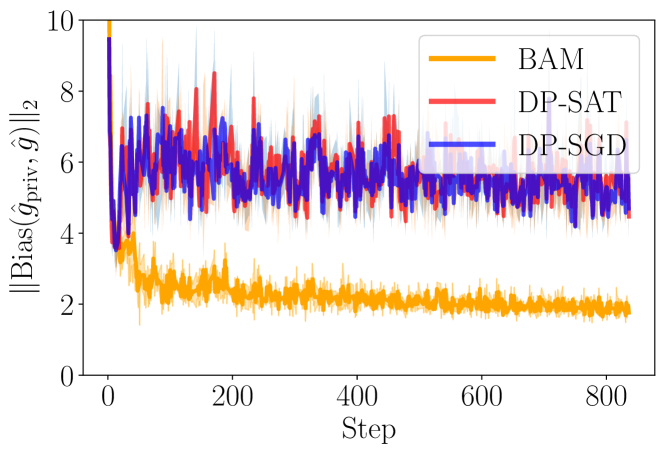
Figure 2: BAM effectively minimises bias: The magnitude of the bias vector measured on CIFAR-10 at a batch size of $512$ is substantially lower for BAM, while DP-SAT incurs the same bias as DP-SGD.

We find that BAM effectively minimises private gradient bias in practice (see Fig. 2 above). On the other hand, DP-SAT largely has no effect on estimator bias for values of the regularisation parameter $\lambda$ that yield high-performing models. Further empirical run-time comparisons (data shown in Appendix A) reveal that while both exact and approximate gradient computations for BAM do incur higher computational costs than DP-SAT (and DP-SGD), this burden is manageable for most practically sized networks with less than 200 layers. Finally, our empirical performance comparison reveals that when using very large batch sizes and the other SOTA practices of De et al. [22], performance gains on more challenging datasets realised through DP-SAT are smaller than reported in the original publication [12]. In contrast, BAM consistently improves performance across different privacy budgets (Table 1).

8 Discussion

After deriving the bias of the private gradient oracle from first principles, we developed a bias-aware regularisation objective $\mathcal{L}_{\mathrm{BAO}}$ that was empirically confirmed effective at minimising the bias vector associated with private gradient estimation. We further demonstrated that using the SAM approximation as suggested by [16], our objective and its gradient are computable with manageable computational overhead.

Our method performs the local gradient ascent step (SAM step) at the per-sample level and is thus closely related to the DP-SAT method of [12], which performs the ascent step with the previous iteration’s privatised mini-batch gradient. Our experiments show that our method outperforms DP-SAT at minimising bias, which is mirrored in the superior accuracy of models trained with BAM. Notably, our method yields a more than $5\%$ accuracy increase on the most challenging dataset tested, ImageNet32. Based on our results, we hypothesise that, with modern private training practices [22] (very large batch size, large learning rate), the noisy gradient of the previous iteration ($\hat{g}^{(t-1)}_{\mathrm{priv}}$), is a poor approximation for finding the maximum loss in the local neighbourhood around the current iteration’s parameter value $\theta^{(t)}$. This is corroborated by a simple experiment (data shown in Fig. 4, Appendix A) that shows the ascent step vector used in DP-SAT to point in slightly different directions to the current iteration’s (un-privatised) mini-batch gradient conventionally used in SAM.

Our results, while not without limitations (BAM incurs slight computational overhead), have shown that reducing private gradient bias can lead to effective performance increases on challenging image datasets. More extensive empirical evaluation, especially on large-scale datasets such as (full-size) ImageNet, is ongoing work and required to fully assess its benefits. Finally, future work should investigate the effectiveness of alternative methods that encourage smoothness [23] and look into connections to and impact on model fairness with respect to sub-groups [24].

9 Acknowledgments

This paper was supported by the DAAD programme Konrad Zuse Schools of Excellence in Artificial Intelligence, sponsored by the Federal Ministry of Education and Research.

Dataset	Method	$\lambda$	Model	Batch-size	LR	C	Multiplicity
CIFAR-10	DP-SGD	$0.0$	ResNet-9	$32\times 128$	2e-3	$1$	16
	DP-SAT	$0.086$
	BAM	$0.02$
CIFAR-100	DP-SGD	$0.0$	ResNet-9	$32\times 128$	2e-3	$1$	16
	DP-SAT	$0.086$
	BAM	$0.01$
ImageNet32	DP-SGD	$0.0$	WideResNet-16-4	$8\times 512$	1e-3	$1$	4
	DP-SAT	$0.07$
	BAM	$0.005$

Table 2: Hyperparameter values for experiments on CIFAR-10, CIFAR-100 and ImageNet32.

Appendix A Experimental details & further results

To obtain suitable hyperparameter values for the compared methods (reported above in Table 2), a random search was first employed using DP-SGD, after which a separate search for optimal $\lambda$-values was performed for both DP-SAT and BAM with N=200 random trials each. For Imagenet32, only a very small-scale hyperparameter search was employed due to the high computational cost. Augmentation multiplicity, as described in [22], was employed with probability $p=0.5$ (for each augmentation) across all compared methods with random pixel shifts (up to $4$ pixels) and random vertical flips. All models were trained for $75$ epochs with the NAdam[25] optimizer and, besides the learning rate (LR), otherwise, default hyperparameters. To meet the different $(\varepsilon,\delta)$ privacy budget requirements the noise multiplier $\sigma^{2}$ was adjusted accordingly.

A.1 Computational aspects

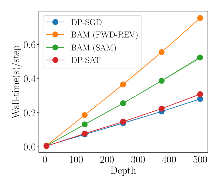
Figure 3: Per-step wall-time (mean $\pm$ SD) for different computational approaches to bias mitigation in DP-SGD for increasing network depth. Results were computed over ten trials and five repetitions.

We evaluate the empirical run-time complexity of the two previously mentioned approaches to compute $\nabla_{\theta}\mathcal{L}_{\mathrm{BAO}}(\theta,x_{i},y_{i})$. Concretely, we compare forward-over-reverse mode AD (BAM FWD-REV) and the SAM (BAM SAM) approximation to compute necessary gradients for BAM and compare to DP-SAT [12]. DP-SAT uses the previous step’s privatised mini-batch gradient to approximate (12) at no additional privacy cost and little computational overhead. Figure 3 showcases the results of an empirical run-time comparison on a toy dataset, implemented in jax [26] and compiled with XLA to obtain a fair comparison between methods.

A.2 Gradient ascent step effectiveness

To investigate the effectiveness the gradient ascent step in DP-SAT and BAM, we investigate the cosine similarity between the ascent direction used by the respective method and the (ground-truth) ascent direction as used in SAM, that is the un-privatised, current mini-batch gradient. Our findings (below in Fig. 4) indicate that the per-sample gradient ascent step of DP-SAT is substantially better aligned with the non-private SAM ascent step than the ascent step with the previous iteration’s privatised gradient of the DP-SAT method. Concretely, we find DP-SAT ascent steps to point in slightly opposite directions, as indicated by a small, but negative cosine similarity.

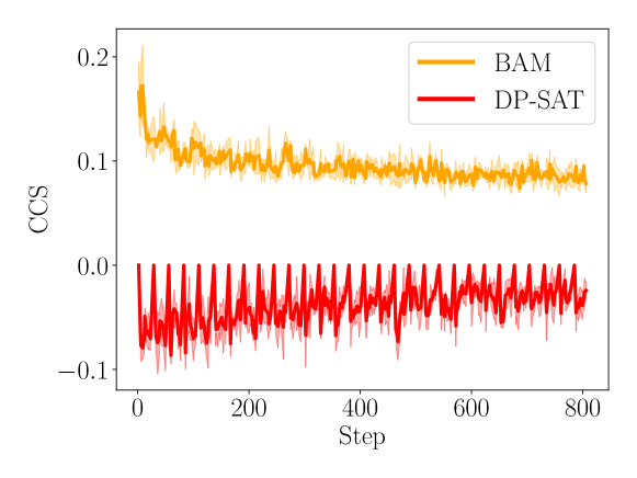
Figure 4: Effectiveness of the ascent step throughout training on CIFAR-10 (three repetitions) with DP-SAT and BAM as measured by the cosine similarity $\mathrm{cos}(\hat{g}_{\mathrm{priv}}^{(t-1)},\hat{g}^{(t)})$ and $1/l\sum_{i}^{l}\mathrm{cos}(g_{i}^{(t)},\hat{g}^{(t)})$ respectively.

A.3 C. Batch size and its effects on bias and directional error

To investigate the empirical success of recent works using extremely large batch sizes (or even full-batch training), we investigate the impact of batch size on private gradient bias and its directional component.

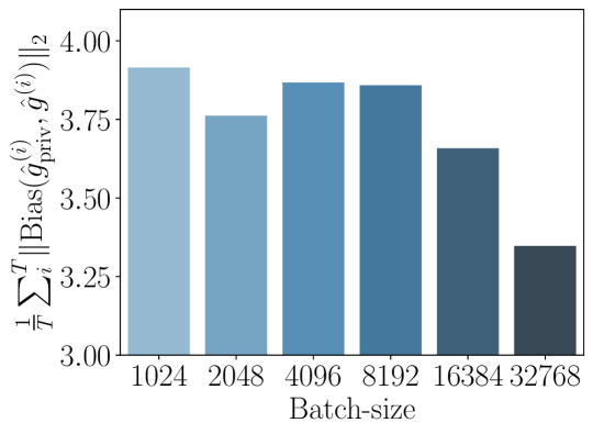
Figure 5: Bigger batches reduce private gradient bias magnitude. The figure showcases bias magnitude averaged over training iterations when training on CIFAR-10 with DP-SGD with different batch sizes.

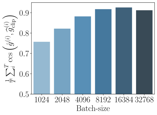
Figure 6: Bigger batches reduce the directional component of private gradient bias as measured by an increased average cosine similarity between clipped and unclipped mini-batch gradients during training on CIFAR-10.

We find large batches to reduce both: the magnitude of the bias vector and the directional components of the bias vector. The latter is indicated by an increased cosine similarity between clipped and unclipped gradients.

Appendix B BAM and effects on loss landscape flatness

Minimising (9) has the additional benefit of smoothing the optimisation landscape around the minima (flat minima) which, as originally argued by Hochreiter and Schmidhuber [27], is widely believed to offer better generalisation performance than sharp minima. To find such flat minima, Zhao et al. [16] propose the objective:

$$\mathcal{L}_{Z}(\theta) =\mathcal{L}(\theta)+\lambda\big{\lVert}\nabla_{\theta}\mathcal{L}(\theta)\big{\rVert}_{2}$$ (15)

$$=\mathcal{L}(\theta)+\lambda\Big{\lVert}\frac{1}{n}\sum_{i=1}^{n}g_{i}\Big{\rVert}_{2}$$ (16)

This objective finds flat minima because $\lVert\nabla_{\theta}\mathcal{L}(\theta)\rVert_{2}$ approximates the Lipschitz constant of the loss function $\mathcal{L}$. The Lipschitz constant is an upper bound on how much the magnitude of a change in the parameter space changes the magnitude of the loss. This is a way of capturing flatness: the smaller the Lipschitz constant of the loss function, the flatter the minima (since the same change in $\theta$ would lead to a smaller bound on the change in the loss magnitude). Hence, by decreasing the Lipschitz constant of the loss function, the solution will be driven towards a flatter minimum.

However, objective (15) cannot be used in our case because it does not allow for the per-sample analysis required for DP. Nonetheless, we can show the following:

Lemma 3.

The bias aware objective $\mathcal{L}_{\mathrm{BAO}}$ (9) upper-bounds the objective $\mathcal{L}_{Z}$ (15) of [16].

Proof.

This follows from the triangle inequality:

$$\mathcal{L}(\theta)+\lambda\Big{\lVert}\frac{1}{n}\sum_{i=1}^{n}g_{i}\Big{\rVert}_{2} =\mathcal{L}(\theta)+\lambda\frac{1}{n}\Big{\lVert}\sum_{i=1}^{n}g_{i}\Big{\rVert}_{2}$$ (17)

$$\leq\mathcal{L}(\theta)+\lambda\frac{1}{n}\sum_{i=1}^{n}\lVert g_{i}\rVert_{2}.$$ (18)

∎

Thus, minimising $\mathcal{L}_{\mathrm{BAO}}$ will additionally drive the solution to a flat minimum by minimising an upper bound on (15).

Appendix C A meaningful decomposition of the private gradient

Figure 7: Illustration of the proposed bias (a) decomposition into orthogonal vector components (b): magnitude $\boldsymbol{a}$ and direction $\boldsymbol{c}$.

With the aim of better capturing the pathological nature of clipping during private stochastic optimisation, we propose a bias decomposition into orthogonal components that allow for the isolation of magnitude and directional estimation error.

In our case, we have an estimator $\hat{g}_{\mathrm{priv}}$ of $\hat{g}$. We now show a decomposition of $\hat{g}_{\mathrm{priv}}$ in terms of $\hat{g}$, which will allow us to differentiate harmful from harmless bias.

Theorem 1.

The private gradient estimate $\hat{g}_{\mathrm{priv}}$ can be decomposed as:

$$\hat{g}_{\mathrm{priv}}=a\cdot\hat{g}+c,$$

where $a\in\mathbb{R},c\in\mathbb{R}^{d}$. We call $a$ the magnitude error and $c$ the directional error that arise through (private) estimation.

Proof.

We first relate each per-sample gradient $g_{i}$ to the mini-batch gradient $\hat{g}$ through a vector decomposition into orthogonal components.

$$g_{i}=\mathrm{proj}_{\hat{g}}\,g_{i}+\tau_{i}$$

where $\mathrm{proj}_{\hat{g}}\,g_{i}=\frac{\langle g_{i},\hat{g}\rangle}{\lVert\hat{g}\rVert^{2}}\cdot\hat{g}$ and $\tau_{i}$ is a suitable vector orthogonal to the projection. Letting $\eta_{i}=\frac{\langle g_{i},\hat{g}\rangle}{\lVert\hat{g}\rVert^{2}}$, the decomposition is:

$$\mathrm{proj}_{\hat{g}}\,g_{i}=\eta_{i}\cdot\hat{g}+\tau_{i}.$$ (19)

Utilising this decomposition inside the $\mathrm{clip}$ function gives us:

$$\mathrm{clip}(g_{i})=\frac{g_{i}}{\max(1,\frac{C}{||\hat{g}_{i}||_{2}})}=\frac{\eta_{i}\hat{g}+\tau_{i}}{\max(1,\frac{C}{||g_{i}||_{2}})}.$$ (20)

Now, let $M_{i}=\max(1,\frac{C}{||g_{i}||_{2}})$ so that we can simplify the above as

$$\mathrm{clip}(g_{i})=\frac{\eta_{i}}{M_{i}}\hat{g}+\frac{\tau_{i}}{M_{i}}.$$ (21)

Averaging the clipped gradients across the mini-batch yields:

$$\hat{g}_{\mathrm{clip}} =\frac{1}{l}\sum_{i=1}^{l}\mathrm{clip}(g_{i})$$ (22)

$$=\frac{1}{l}\sum_{i=1}^{l}\left(\frac{\eta_{i}}{M_{i}}\hat{g}+\frac{\tau_{i}}{M_{i}}\right)$$ (23)

$$=\left(\frac{1}{l}\sum_{i=1}^{l}\frac{\eta_{i}}{M_{i}}\right)\;\cdot\;\hat{g}+\left(\frac{1}{l}\sum_{i=1}^{l}\frac{\tau_{i}}{M_{i}}\right).$$ (24)

Finally, perturbing each $g_{i}$ with a vector $\beta_{i}\sim\mathcal{N}(0,C\sigma I_{d})$ we obtain the desired decomposition in terms of magnitude error $a$ and directional error $c$:

$$\hat{g}_{\mathrm{priv}} =\frac{1}{l}\sum_{i=1}^{l}\left(\mathrm{clip}(g_{i})+\beta_{i}\right)$$ (25)

$$=\underbrace{\left(\frac{1}{l}\sum_{i=1}^{l}\frac{\eta_{i}}{M_{i}}\right)}_{a}\;\cdot\;\hat{g}\;+\;\underbrace{\left(\frac{1}{l}\sum_{i=1}^{l}\frac{\tau_{i}}{M_{i}}+\beta_{i}\right)}_{c}$$ (26)

∎

This allows us to now effectively isolate directional from magnitude components of the private gradient bias:

$$\mathrm{Bias}(\hat{g}_{\mathrm{priv}},\hat{g}) =\mathbb{E}\left[\hat{g}_{\mathrm{priv}}\right]-\hat{g}$$ (27)

$$=\mathbb{E}\left[a\cdot\hat{g}+c\right]-\hat{g}.$$ (28)

References

- Geiping et al. [2020] Jonas Geiping, Hartmut Bauermeister, Hannah Dröge, and Michael Moeller. Inverting gradients-how easy is it to break privacy in federated learning? Advances in Neural Information Processing Systems, 33:16937–16947, 2020.
- Carlini et al. [2021] Nicholas Carlini, Florian Tramer, Eric Wallace, Matthew Jagielski, Ariel Herbert-Voss, Katherine Lee, Adam Roberts, Tom Brown, Dawn Song, Ulfar Erlingsson, et al. Extracting training data from large language models. In 30th USENIX Security Symposium (USENIX Security 21), pages 2633–2650, 2021.
- Carlini et al. [2019] Nicholas Carlini, Chang Liu, Úlfar Erlingsson, Jernej Kos, and Dawn Song. The secret sharer: Evaluating and testing unintended memorization in neural networks. In 28th USENIX Security Symposium (USENIX Security 19), pages 267–284, 2019.
- Dwork et al. [2014a] Cynthia Dwork, Aaron Roth, et al. The algorithmic foundations of differential privacy. Foundations and Trends® in Theoretical Computer Science, 9(3–4):211–407, 2014a.
- Shokri and Shmatikov [2015] Reza Shokri and Vitaly Shmatikov. Privacy-preserving deep learning. In Proceedings of the 22nd ACM SIGSAC conference on computer and communications security, pages 1310–1321, 2015.
- Abadi et al. [2016] Martin Abadi, Andy Chu, Ian Goodfellow, H Brendan McMahan, Ilya Mironov, Kunal Talwar, and Li Zhang. Deep learning with differential privacy. In Proceedings of the 2016 ACM SIGSAC conference on computer and communications security, pages 308–318, 2016.
- McMahan et al. [2018] H Brendan McMahan, Daniel Ramage, Kunal Talwar, and Li Zhang. Learning differentially private recurrent language models. In International Conference on Learning Representations, 2018.
- Zhang et al. [2019] Jingzhao Zhang, Tianxing He, Suvrit Sra, and Ali Jadbabaie. Why gradient clipping accelerates training: A theoretical justification for adaptivity. In International Conference on Learning Representations, 2019.
- Qian et al. [2021] Jiang Qian, Yuren Wu, Bojin Zhuang, Shaojun Wang, and Jing Xiao. Understanding gradient clipping in incremental gradient methods. In International Conference on Artificial Intelligence and Statistics, pages 1504–1512. PMLR, 2021.
- Song et al. [2020] Shuang Song, Om Thakkar, and Abhradeep Thakurta. Characterizing private clipped gradient descent on convex generalized linear problems. arXiv preprint arXiv:2006.06783, 2020.
- Chen et al. [2020] Xiangyi Chen, Steven Z Wu, and Mingyi Hong. Understanding gradient clipping in private sgd: A geometric perspective. Advances in Neural Information Processing Systems, 33:13773–13782, 2020.
- Park et al. [2023] Jinseong Park, Hoki Kim, Yujin Choi, and Jaewook Lee. Differentially private sharpness-aware training. In International Conference on Machine Learning, pages XXXX–YYYY. PMLR, 2023.
- Shi et al. [2023] Yifan Shi, Yingqi Liu, Kang Wei, Li Shen, Xueqian Wang, and Dacheng Tao. Make landscape flatter in differentially private federated learning. In Proceedings of the IEEE/CVF Conference on Computer Vision and Pattern Recognition, pages 24552–24562, 2023.
- Foret et al. [2020] Pierre Foret, Ariel Kleiner, Hossein Mobahi, and Behnam Neyshabur. Sharpness-aware minimization for efficiently improving generalization. arXiv preprint arXiv:2010.01412, 2020.
- Dwork et al. [2014b] Cynthia Dwork, Aaron Roth, et al. The algorithmic foundations of differential privacy. 2014b.
- Zhao et al. [2022] Yang Zhao, Hao Zhang, and Xiuyuan Hu. Penalizing gradient norm for efficiently improving generalization in deep learning. In International Conference on Machine Learning, pages 26982–26992. PMLR, 2022.
- Karakida et al. [2022] Ryo Karakida, Tomoumi Takase, Tomohiro Hayase, and Kazuki Osawa. Understanding gradient regularization in deep learning: Efficient finite-difference computation and implicit bias. arXiv preprint arXiv:2210.02720, 2022.
- Wiltschko and Johnson [n.d.] Alex Wiltschko and Matthew Johnson. Jax- autodiff cookbook, n.d. Accessed June 20, 2023. https://jax.readthedocs.io/en/latest/notebooks/autodiff˙cookbook.html.
- Pearlmutter [1994] Barak A Pearlmutter. Fast exact multiplication by the hessian. Neural computation, 6(1):147–160, 1994.
- Krizhevsky et al. [2009] Alex Krizhevsky, Geoffrey Hinton, et al. Learning multiple layers of features from tiny images. 2009.
- Chrabaszcz et al. [2017] Patryk Chrabaszcz, Ilya Loshchilov, and Frank Hutter. A downsampled variant of imagenet as an alternative to the cifar datasets. arXiv preprint arXiv:1707.08819, 2017.
- De et al. [2022] Soham De, Leonard Berrada, Jamie Hayes, Samuel L Smith, and Borja Balle. Unlocking high-accuracy differentially private image classification through scale. arXiv preprint arXiv:2204.13650, 2022.
- Cha et al. [2021] Junbum Cha, Sanghyuk Chun, Kyungjae Lee, Han-Cheol Cho, Seunghyun Park, Yunsung Lee, and Sungrae Park. Swad: Domain generalization by seeking flat minima. Advances in Neural Information Processing Systems, 34:22405–22418, 2021.
- Tran et al. [2021] Cuong Tran, My Dinh, and Ferdinando Fioretto. Differentially private empirical risk minimization under the fairness lens. Advances in Neural Information Processing Systems, 34:27555–27565, 2021.
- Dozat [2016] Timothy Dozat. Incorporating nesterov momentum into adam. 2016.
- Bradbury et al. [2018] James Bradbury, Roy Frostig, Peter Hawkins, Matthew James Johnson, Chris Leary, Dougal Maclaurin, George Necula, Adam Paszke, Jake VanderPlas, Skye Wanderman-Milne, and Qiao Zhang. JAX: composable transformations of Python+NumPy programs, 2018. URL http://github.com/google/jax.
- Hochreiter and Schmidhuber [1997] Sepp Hochreiter and Jürgen Schmidhuber. Flat minima. Neural computation, 9(1):1–42, 1997.