Negative Refraction in isotropic achiral and chiral materials

Abstract

We show that negative refraction in materials can occur at frequencies $\omega$ where the real part of the permittivity $\varepsilon(\omega)$ and the real part of the permeability $\mu(\omega)$ are of different sign, and that light with such frequencies can propagate just as well as light with frequencies where they are of equal sign. Therefore, in order to have negative refraction one does not need to be in the “double negative” regime. We consider negative refractive index achiral materials using the Drude model, and chiral materials using the Drude-Born-Fedorov model. We find that the time-averaged Poynting vector always points along the wave vector, the time-averaged energy flux density is always positive, and the time-averaged energy density is positive (negative) when the refractive index is positive (negative). The phase velocity is negative when the real part of the refractive index is negative, and the group velocity generally changes sign several times as a function of frequency near resonance.

Introduction: Negative refraction (NR) is a phenomenon in which electromagnetic waves are refracted at an interface with NR angle [1, 2, 3, 4, 5]. It is believed that in order for NR to occur, the real part of the (electric) permittivity ($\varepsilon$) and real part of the (magnetic) permeability ($\mu$) must both be negative at a particular frequency [1, 2, 3, 4, 5, 6, 7, 8, 9]. Such materials are sometimes called “double negative” materials. NR meta-materials, i.e., specially designed double negative materials made from assemblies of multiple elements fashioned from composite materials have been developed [3, 6, 7, 8, 9]. It is furthermore believed that light at frequencies such that {${\mathrm{Re}}(\varepsilon(\omega))>0$ and ${\mathrm{Re}}(\mu(\omega))<0$} or {${\mathrm{Re}}(\varepsilon(\omega))<0$ and ${\mathrm{Re}}(\mu(\omega))>0$}, is not able to propagate in materials [1, 2, 3, 4, 5, 6, 7, 8, 9]. Here we show that both beliefs are false. We shall use the amplitude-phase representation of the permittivity and permeability within a Drude model to calculate the complex refractive index. We then analyze and categorize the wealth of phenomena in isotropic achiral and chiral media that occur when optical waves in frequency ranges near resonant optical transitions where NR is possible.

NR materials are usually man-made meta-materials, but naturally occurring NR materials exist, e.g., Dirac semi-metals such as Cd₃As₂ [10]. NR meta-materials have led to significant technological advancements [4, 5, 6, 7, 8, 9] including: (1) superlensing, i.e., overcoming the diffraction limit of conventional lenses, allowing for sub-wavelength imaging for high-resolution microscopy [11, 12], (2) cloaking using devices that can manipulate the flow of light around an object, rendering it invisible to observers [4, 13, 14], (3) terahertz imaging, spectroscopy, and communication systems, enabling non-invasive inspections in biomedical imaging and security screening [15], (4) antennas incorporating NR meta-materials that can enhance the radiated power of the antenna NR by focusing electromagnetic radiation by a flat lens versus dispersion [16, 17, 18].

Theory: For an electromagnetic plane wave, $\mathbf{E}({\bf r},t)=\mathrm{Re}(\bm{\mathcal{E}}_{0}\,e^{i(\mathbf{k}\cdot\mathbf{r}-\omega t)})$ and $\mathbf{H}({\bf r},t)=\mathrm{Re}(\bm{\mathcal{H}}_{0}\,e^{i(\mathbf{k}\cdot\mathbf{r}-\omega t)})$, the Faraday and Ampère equations, together with the constitutive equations ${\bf D}=\varepsilon{\bf E}$ and ${\bf B}=\mu{\bf H}$ in an isotropic homogeneous material, yield, in SI units,

$${\bf k}\times\bm{\mathcal{E}}_{0}=\omega\,\mu(\omega)\bm{\mathcal{H}}_{0},\quad{\bf k}\times\bm{\mathcal{H}}_{0}=-\omega\,\varepsilon(\omega)\bm{\mathcal{E}}_{0}.$$ (1)

Substituting ${\bf k}=\tfrac{n(\omega)\,\omega}{c}\,{\hat{\bf k}}$ we obtain

$$n(\omega)\,{\hat{\bf k}}\times\bm{\mathcal{E}}_{0}=c\,\mu(\omega)\bm{\mathcal{H}}_{0},$$ (2)

$$n(\omega)\,{\hat{\bf k}}\times\bm{\mathcal{H}}_{0}=-c\,\varepsilon(\omega)\bm{\mathcal{E}}_{0},$$ (3)

which yields [noting that in vacuum, $c^{2}=(\varepsilon_{0}\mu_{0})^{-1}$],

$$n^{2}(\omega)=c^{2}\varepsilon(\omega)\mu(\omega)=\tfrac{\varepsilon(\omega)\mu(\omega)}{\varepsilon_{0}\mu_{0}}.$$ (4)

The Drude(-Lorentz) model [19] is a widely used theoretical framework for describing the behavior of electromagnetic waves in materials. It provides a phenomenological approach to model $\varepsilon$ and $\mu$ of materials, including those with NR. In the Drude model, the equation of motion for an electron in a meta-atom can be expressed as:

$$m\frac{d^{2}\mathbf{r}}{dt^{2}}=-m\omega_{0}^{2}\mathbf{r}-m\gamma\frac{d\mathbf{r}}{dt}+(-e)\mathbf{E}(\omega)e^{-i\omega t},$$ (5)

where $m$ is the effective mass of the electron, $\mathbf{r}(t)$ is the displacement of the electron, $\omega_{0}$ is the resonance frequency, $\gamma$ is the damping coefficient, $e$ is the elementary charge, and $\mathbf{E}(\omega)$ is the electric field of the incident electromagnetic wave at frequency $\omega$. Substituting $\mathbf{r}(t)=\mathbf{r}_{0}(\omega)e^{-i\omega t}$, into Eq. (5), we find $\mathbf{r}_{0}(\omega)=\left(\frac{-e/m}{\omega_{0}^{2}-\omega^{2}+i\gamma\omega}\right)\mathbf{E}(\omega)$. The polarization $\mathbf{P}(\omega)$ related to the induced dipole moment per unit volume, can be written as $\mathbf{P}(\omega)=Ne\mathbf{r}_{0}(\omega)\equiv\chi(\omega)\mathbf{E}(\omega)$, where $\chi(\omega)$ is the electric susceptibility of the material. Substituting the expression for $\mathbf{r}_{0}$ into $\mathbf{P}(\omega)$, we can obtain the electric susceptibility as $\chi(\omega)=-\frac{Ne^{2}}{m(\omega^{2}-\omega_{0}^{2}+i\gamma\omega)}$ where $N$ is the number density of electric dipole moments. The electric permittivity $\varepsilon(\omega)$ of the material can then be calculated as $\varepsilon(\omega)=\varepsilon_{0}(1+\chi(\omega))=\varepsilon_{0}(1-\frac{\omega_{p}^{2}}{\omega^{2}-\omega_{0}^{2}+i\gamma\omega})$ where the plasma frequency is defined by $\omega_{p}^{2}=\frac{Ne^{2}}{m}$ [20]. Similarly, a magnetic dipole transition with resonance frequency $\omega_{0}^{\prime}$ and width $\gamma^{\prime}$ yields the magnetic permeability $\mu(\omega)=\mu_{0}(1-\frac{\omega_{p,m}^{2}}{\omega^{2}-\omega_{0}^{\prime 2}+i\gamma^{\prime}\omega})$ where the magnetic plasma frequency squared, $\omega_{p,m}^{2}$, is a constant related to the magnetic properties of the material and is proportional to the transition magnetic dipole moment squared.

In order to develop the theory of NR, Veselago [1] wrote, $n(\omega)=\pm\sqrt{\tfrac{\varepsilon(\omega)\mu(\omega)}{\varepsilon_{0}\mu_{0}}}$, where the minus sign is required for the case when the real part of both $\varepsilon(\omega)$ and $\mu(\omega)$ are negative. This is the standard approach for dealing with double negative materials [1, 2, 3, 4, 5, 6, 7, 8, 9]. Instead we follow a more direct and mathematically appealing procedure. We write the complex refractive index as

$$n(\omega)=\frac{\sqrt{|\varepsilon(\omega)||\mu(\omega)|}}{\sqrt{\varepsilon_{0}\mu_{0}}}e^{i(\theta_{\varepsilon}(\omega)+\theta_{\mu}(\omega))/2},$$ (6)

where $\theta_{\varepsilon}$ and $\theta_{\mu}$ are the complex phase of $\varepsilon$ and $\mu$, respectively, i.e., $\varepsilon=|\varepsilon|e^{i\theta_{\varepsilon}}$, $\mu=|\mu|e^{i\theta_{\mu}}$. This form for the refractive index is unique (there are no branch point problems) because of the square root in the definition of the refractive index. The real (imaginary) part of $n(\omega)$ is the refractive index (optical absorption coefficient divided by $\omega/c$).

The Poynting vector (which gives the electromagnetic energy transfer per unit area per unit time) is defined as $\mathbf{S}=\mathbf{E}\times\mathbf{H}$. For a linearly polarized plane wave with $\mathbf{E}({\bf r},t)=\mathrm{Re}(\bm{\mathcal{E}}_{0}\,e^{i(\mathbf{k}\cdot\mathbf{r}-\omega t)})$ and $\mathbf{H}({\bf r},t)=\mathrm{Re}(\bm{\mathcal{H}}_{0}\,e^{i(\mathbf{k}\cdot\mathbf{r}-\omega t)})$, where $\bm{\mathcal{E}}_{0}$ and $\bm{\mathcal{H}}_{0}$ obey the Eqs. (2) and (3) with $\varepsilon$, $\mu$ and $n$ complex, the three orthogonal vectors {$\bm{\mathcal{E}}_{0},\bm{\mathcal{H}}_{0},\mathbf{k}$}, can be written as $\bm{\mathcal{E}}_{0}=\!\mathcal{E}_{0}\,\hat{\mathbf{x}}$, $\bm{\mathcal{H}}_{0}=\mathcal{H}_{0}\,\hat{\mathbf{y}}$ and $\mathbf{k}=k\,\hat{\mathbf{z}}$, where $k=\omega n(\omega)/c$, $\mathcal{H}_{0}=\sqrt{|\varepsilon|/|\mu|}\,\mathcal{E}_{0}e^{i\theta_{H}}$, and $\theta_{H}=(\theta_{\varepsilon}-\theta_{\mu})/2$. The orthogonal vectors {$\bm{\mathcal{E}}_{0},\bm{\mathcal{H}}_{0},\mathbf{k}$} form a right(left)-handed coordinate system if $\mathrm{Re}(n)>0$ ($\mathrm{Re}(n)<0$). Taking $\mathcal{E}_{0}$ to be real and positive, we obtain $\mathbf{S}=\hat{\mathbf{z}}\,\sqrt{|\varepsilon|/|\mu|}\,\mathcal{E}_{0}^{2}\cos(\zeta)\cos(\zeta+\theta_{H})e^{-2k^{\prime\prime}z}$. Here $\zeta=k^{\prime}z-\omega t$, and $k^{\prime}=n^{\prime}(\omega)\omega/c$ ($k^{\prime\prime}=n^{\prime\prime}(\omega)\omega/c$) is the real (imaginary) part of $k$, and $n^{\prime}$ ($n^{\prime\prime}$) is the real (imaginary) part of $n$. When $\theta_{H}$ vanishes, $\mathbf{S}$ is proportional to $\cos^{2}(\zeta)$ and is directed along $\hat{\mathbf{z}}$. When $\theta_{H}\neq 0$, the magnetic field has the phase shift $\theta_{H}$ with respect to the electric field. Hence, there are intervals of $\zeta$ where both $\cos(\zeta)$ and $\cos(\zeta+\theta_{H})$ have the same sign and $\mathbf{S}$ is along $\hat{\mathbf{z}}$, and there are intervals of $\zeta$ where $\cos(\zeta)$ and $\cos(\zeta+\theta_{H})$ have different signs. In the latter case, $\mathbf{S}$ is along $-\hat{\bf z}$. Hence the energy transfer per unit area per unit time is time-dependent and can be either positive or negative. The time-averaged energy flux is $\bar{\mathbf{S}}\equiv\tfrac{1}{T}\int_{0}^{T}\mathbf{S}(z,t)dt=\hat{\mathbf{z}}\,\sqrt{|\varepsilon|/|\mu|}\,(\mathcal{E}_{0}^{2}/2)\cos(\theta_{H})e^{-2k^{\prime\prime}z}$, where $T=2\pi/\omega$ is the wave period. Since $0\leq\theta_{\varepsilon}<\pi$ and $0\leq\theta_{\mu}<\pi$, and $|\theta_{H}|\leq\pi/2$, as is clear from the Drude model, $\bar{\mathbf{S}}$ is always directed along $\hat{\mathbf{z}}$.

The electromagnetic energy density is $u=(\mathbf{E}\cdot\mathbf{D}+\mathbf{B}\cdot\mathbf{H})/2$. Taking into account that $\mathbf{D}=\mathrm{Re}(\varepsilon\bm{\mathcal{E}})$, we can write the electric energy density as $\mathbf{E}\cdot\mathbf{D}/2=\tfrac{|\varepsilon|}{2}\mathcal{E}_{0}^{2}\cos(\zeta)\cos(\zeta+\theta_{\varepsilon})\,e^{-2k^{\prime\prime}z}$. When $\varepsilon$ is real and positive, $\theta_{\varepsilon}$ vanishes and $\mathbf{E}\cdot\mathbf{D}$ is positive. For complex $\varepsilon$, $\theta_{\varepsilon}\neq 0$, and there are intervals of $\zeta$ where $\mathbf{E}\cdot\mathbf{D}$ is negative. The negative sign of $\mathbf{E}\cdot\mathbf{D}$ occurs due to interaction of light with frequency $\omega$ which is close to the dipole electric transition frequency $\omega_{0}$. Similarly, $\mathbf{B}=\mathrm{Re}(\mu\bm{\mathcal{H}})$, and the magnetic energy density is $\mathbf{B}\cdot\mathbf{H}/2=\tfrac{|\varepsilon|}{2}\mathcal{E}_{0}^{2}\cos(\zeta+\theta_{H})\cos(\zeta+\theta_{n})\,e^{-2k^{\prime\prime}z}$, where $\theta_{n}=(\theta_{\varepsilon}+\theta_{\mu})/2$ [see Eq. (6]. When $\mu$ is real and positive, $\theta_{\mu}=0$, and $\theta_{H}=\theta_{n}=\theta_{\varepsilon}/2$, hence $\mathbf{B}\cdot\mathbf{H}$ is positive. For complex $\mu$, $\theta_{H}\neq\theta_{n}$, and there are intervals of $\zeta$ where $\mathbf{B}\cdot\mathbf{H}$ is negative. The negative sign of $\mathbf{B}\cdot\mathbf{H}$ occurs due to interaction of light with frequency $\omega$ close to the dipole magnetic transition frequency $\omega^{\prime}_{0}$. The electromagnetic energy density is $u=\frac{|\varepsilon|}{2}\mathcal{E}_{0}^{2}\big{[}\cos(\zeta)\cos(\zeta+\theta_{\varepsilon})+\cos(\zeta+\theta_{H})\cos(\zeta+\theta_{n})\big{]}e^{-2k^{\prime\prime}z}$, and its average over a period $T$ is $\bar{u}\equiv\tfrac{1}{T}\int_{0}^{T}u(z,t)dt=\tfrac{|\varepsilon|}{2}\mathcal{E}_{0}^{2}\cos\theta_{n}\cos\theta_{H}$. Note that $\bar{u}<0$ over the frequency region where ${\mathrm{Re}}[n]<0$ [21, 22]. See the SM [21] figure in the section titled Energy Density which shows the frequency region where both the average energy density and the refractive index are negative. Note that when the electromagnetic wave propagates in a medium with real $n(\omega)$, $\mathbf{S}(z,t)$ and $u(z,t)$ satisfy the Poynting theorem, $\partial_{t}u(z,t)+\nabla\cdot\mathbf{S}(z,t)=0$. When $n(\omega)$ is complex, $\mathbf{S}(z,t)$ and $u(z,t)$ undergo exponential decay as described by the Beer–Lambert law.

The phase velocity of light is $v_{p}=\omega/k^{\prime}$, and the group velocity is $v_{g}=(\partial k^{\prime}/\partial\omega)^{-1}$/ Hence, $v_{p}=c/n^{\prime}$, and $v_{g}=c/(n^{\prime}+\omega\partial_{\omega}n^{\prime})$. Note that when $n^{\prime}<0$, the phase velocity is negative, and when $n^{\prime}+\omega\partial_{\omega}n^{\prime}<0$, the group velocity is negative. In other words, if a pulse propagates through a material with a negative group velocity, the peak of the pulse propagates in the direction opposite to the energy flow direction [24, 23]. Moreover, near a resonance, $n^{\prime}+\omega\partial_{\omega}n^{\prime}$ can be small, and the group velocity can exceed the speed of light [25]. Experiments have verified that it is possible for the group velocity to exceed the speed of light in vacuum [26, 24, 27, 28].

A circular-polarization representation for achiral materials will be discussed following the chiral case below. It turns out to be simpler than the linearly polarized analysis above.

Numerical results: Using the Drude model for an electric dipole transition and a magnetic dipole transition with resonance frequencies that are close to one another (see the caption of Fig. 1 for the set of parameters used), we calculate the complex permittivity $\varepsilon(\omega)$ and complex permeability $\mu(\omega)$ versus frequency, and the complex refractive index $n(\omega)$ (whose real part is the index of refraction and imaginary part is the absorption coefficient) using Eq. (6). Figure 1 shows the complex $\varepsilon(\omega)$ and $\mu(\omega)$ versus frequency calculated with the Drude model. The region of frequencies where both of the real parts of $\varepsilon(\omega)$ and $\mu(\omega)$ are negative in Fig. 1, but there are also frequency regions where the real parts of $\varepsilon(\omega)$ and $\mu(\omega)$ are of opposite sign. Figure 2 plots the real and imaginary parts $n(\omega)$, defined in Eq. (6), versus $\omega$. Note that the absorption coefficient $\alpha\equiv\mathrm{Im}[n(\omega)]\geq 0$ for all frequencies [hence there is absorption (no gain) for all frequencies]. Moreover, there are frequency regions where $\mathrm{Re}[n(\omega)]<0$ and in part of this frequency range the real parts of $\varepsilon(\omega)$ and $\mu(\omega)$ are of opposite sign. A figure in [21] shows the the real and imaginary parts $n(\omega)$ plotted versus $\omega$ where these functions are set to zero in the regions where the real parts of $\varepsilon$ and $\mu$ are of opposite sign. In that figure, the region near $\omega=3$ where the functions are zeroed correspond to frequencies to the right of the zero in the real part of $\varepsilon$ and the the left of the frequency where real part of $\mu$ vanishes. The large region where the function are zeroed to the right of $\omega=3.7$ is where the real part of $\varepsilon$ is negative but the real part of $\mu$ is positive.

Figure 1: The complex relative electric permittivity ($\varepsilon/\varepsilon_{0}$) and complex magnetic permeability ($\mu/\mu_{0}$) plotted versus $\omega$ (in arbitrary units) for Drude parameters, $\omega_{0}=3,\omega_{0}^{\prime}=3.2,\gamma=0.3,\gamma^{\prime}=0.2,\omega_{p}=5,\omega_{p,m}=2$. The dashed curves are the imaginary parts of $\varepsilon(\omega)$ and $\mu(\omega)$.

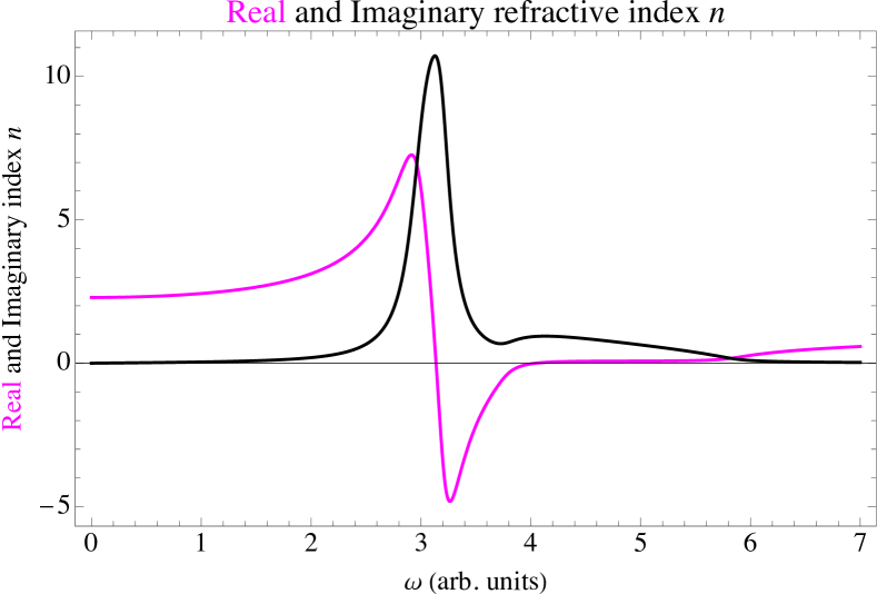
Figure 2: The real (magenta) and imaginary (black) parts of the complex refractive index $n(\omega)$ versus $\omega$ (in arbitrary units) for same Drude parameters as used in Fig. 1. The NR region is right of the resonance frequency. The imaginary part shows absorption over a large region about the resonance frequency.

The supplementary material (SM) [21] contains a Mathematica notebook used to produce the numerical results in Figs. 1 and 2, and Fig. 3; you can vary the parameters of the model by using the sliders in the Manipulate statements in the notebook. For comparison, the SM notebook [21] also calculates and plots $n(\omega)$ assuming the light can propagate only if the real parts of $\varepsilon$ and $\mu$ are the same sign, as assumed in the literature. You can compare this figure with Fig. 2 (and the refractive index figures in the notebook).

Chiral Media: The constitutive equations for isotropic chiral media must be modified to allow for optical activity. One form of the modified constitutive equations, called the Drude-Born-Fedorov model [19, 29], is as follows:

$$\bm{\mathcal{D}} = \varepsilon[\bm{\mathcal{E}}+\beta\,\nabla\times\bm{\mathcal{E}}],$$ (7)

$$\bm{\mathcal{B}} = \mu[\bm{\mathcal{H}}+\beta\,\nabla\times\bm{\mathcal{H}}].$$ (8)

This form is symmetric under time-reversal. The pseudoscalar $\beta$, sometimes called the chiral admittance, has the units of length and is a measure of the optical activity. Let us consider a plane wave electromagnetic field, ${\bf E}({\bf r},t)={\mathrm{Re}}[\bm{\mathcal{E}}({\bf r},t)]={\mathrm{Re}}[\bm{\mathcal{E}}_{0}e^{i({\bf k}\cdot{\bf r}-\omega\,t)}]$, and similarly for ${\bf B}({\bf r},t)$, ${\bf D}({\bf r},t)$ and ${\bf H}({\bf r},t)$, and determine the consequences of Eqs. (7)-(8). Using the Faraday and Ampère laws in a nonconducting medium, $\nabla\times\bm{\mathcal{E}}=i\omega\bm{\mathcal{B}}$, $\nabla\times\bm{\mathcal{H}}=-i\omega\bm{\mathcal{D}}$, the Drude-Born-Fedorov equation takes the form

$$\bm{\mathcal{D}}_{0}=\varepsilon\left[\bm{\mathcal{E}}_{0}+i\omega\beta\bm{\mathcal{B}}_{0}\right],\quad\bm{\mathcal{B}}_{0}=\mu\left[\bm{\mathcal{H}}_{0}-i\omega\beta\bm{\mathcal{D}}_{0}\right],$$ (9)

These equations can be written in matrix form as

$$\left(\begin{matrix}\bm{\mathcal{E}}_{0}\\ \bm{\mathcal{H}}_{0}\\ \end{matrix}\right)=\left(\begin{matrix}\varepsilon^{-1}&-i\omega\beta\\ i\omega\beta&\mu^{-1}\end{matrix}\right)\left(\begin{matrix}\bm{\mathcal{D}}_{0}\\ \bm{\mathcal{B}}_{0}\end{matrix}\right).\,\,\,\,\,\,\,\,$$ (10)

Substituting into the Faraday and Ampère equations gives

$${\bf k}\times\bm{\mathcal{E}}_{0}=\omega\bm{\mathcal{B}}_{0},\qquad{\bf k}\times\bm{\mathcal{H}}_{0}=-\omega\bm{\mathcal{D}}_{0},$$ (11)

which, upon writing ${\bf k}=\tfrac{\tilde{n}(\omega)\omega}{c}\,{\hat{\bf k}}$, can be written in terms of the refractive index as

$$\frac{\tilde{n}(\omega)}{c}\,{\hat{\bf k}}\times(\varepsilon^{-1}\bm{\mathcal{D}}_{0}-i\omega\beta\bm{\mathcal{B}}_{0}) = \bm{\mathcal{B}}_{0},$$

$$\frac{\tilde{n}(\omega)}{c}\,{\hat{\bf k}}\times(\mu^{-1}\bm{\mathcal{B}}_{0}+i\omega\beta\bm{\mathcal{D}}_{0}) = -\bm{\mathcal{D}}_{0}.$$ (12)

Solving for $\tilde{n}(\omega)$ in the determinant obtained using these equations yields two degenerate solutions for the right-and left-handed circularly polarized light fields,

$$\tilde{n}(\omega)\equiv\ n_{\pm}(\omega)=\frac{n(\omega)}{1\mp\frac{\beta\omega}{c}\,n(\omega)},$$ (13)

where $\varepsilon$, $\mu$, $\theta_{\varepsilon}$ and $\theta_{\mu}$ are $\omega$ dependent, and $n(\omega)$ is given in Eq. (6).

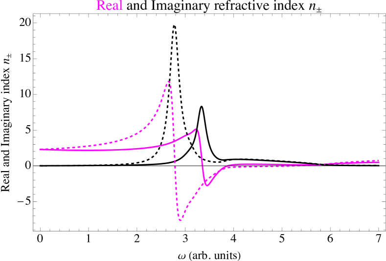
Figure 3: In a medium that is chiral, the real and imaginary parts of the complex refractive index $n_{\pm}(\omega)$ versus $\omega$ (in arbitrary units) are different for right-circular polarization (solid curves) and left (dashed). The same Drude parameters as used in Fig. 1 are used here, and $\beta=0.05$ (arb. units –FIX).

Figure 3 plots the real (magenta) and imaginary (black) parts of $n_{\pm}(\omega)$ versus $\omega$ for right-circular polarized ($+$) (solid curves) and left-circular polarized ($-$) light (dashed curves). The resonance frequency and the entire curves for the complex refractive index are shifted to higher (lower) frequencies for the right-circular polarized (left-circular polarized) light in the chiral medium (finite $\beta$) relative to those in Fig. 2 (which is for $\beta=0$). Moreover, both ${\mathrm{Re}}(n_{+})$ and ${\mathrm{Im}}(n_{+})$ are smaller in magnitude than ${\mathrm{Re}}(n_{-})$ and ${\mathrm{Im}}(n_{-})$, respectively. Clearly, both ${\mathrm{Re}}(n_{+})$ and ${\mathrm{Im}}(n_{-})$ have regions of NR. Also both ${\mathrm{Im}}(n_{+})$ and ${\mathrm{Im}}(n_{-})$ are positive (absorptive) for all frequencies.

Using a circular polarization basis we write

$$\bm{\mathcal{E}}_{0}=\mathcal{E}_{+}\,\mathbf{e}_{+}+\mathcal{E}_{-}\,\mathbf{e}_{-},$$ (14)

(similarly for $\bm{\mathcal{D}}_{0}$, $\bm{\mathcal{B}}_{0}$ and $\bm{\mathcal{H}}_{0}$) where the subscript $\pm$ refers to right-polarized (left-polarized) waves, $\mathbf{e}_{+}=\frac{-1}{\sqrt{2}}\,\big{(}\hat{\mathbf{x}}+i\hat{\mathbf{y}}\big{)}$, and $\mathbf{e}_{-}=\frac{1}{\sqrt{2}}\,\big{(}\hat{\mathbf{x}}-i\hat{\mathbf{y}}\big{)}$. We find that

$$\mathcal{D}_{\pm}=\frac{n_{\pm}(\omega)}{n(\omega)}\,\varepsilon(\omega)\mathcal{E}_{\pm},\quad\mathcal{B}_{\pm}=\mp\frac{in_{\pm}(\omega)}{c}\,\mathcal{E}_{\pm},$$

$$\mathcal{H}_{\pm}=\mp i\sqrt{\frac{|\varepsilon(\omega)|}{|\mu(\omega)|}}\,e^{i\theta_{H}}\mathcal{E}_{\pm}.$$ (15)

The real part of the complex wavenumber of a circularly polarized wave is $k^{\prime}_{\sigma}=\omega n^{\prime}_{\sigma}(\omega)/c$, where $\sigma=\pm$, and $n^{\prime}_{\sigma}(\omega)$ is the real part of $n_{\sigma}(\omega)$. The rotation angle of the polarization of linearly polarized light is given by $\theta_{\mathrm{rot}}=\Delta n_{\pm}l=(n^{\prime}_{+}-n^{\prime}_{-})l$, where $l$ is the length of the NR material traversed. The SM [21] contains a Manipulate statement where you can vary the $\beta$ parameter (and other parameters) and view the dramatic changes in the frequency dependence of $\theta_{\mathrm{rot}}(\omega)$. Moreover, differential absorption $\Delta\alpha_{\pm}\equiv(n^{\prime\prime}_{+}-n^{\prime\prime}_{-})\tfrac{\omega}{c}$ (circular dichroism) ensues, hence the light will generally be elliptically polarized upon propagation through the material, and $\theta_{\mathrm{rot}}(\omega)$ will be the rotation of the major and minor axes. Note that $\beta$ itself might be frequency dependent but it is not clear how to model such dependence at present. The phase velocity is $v_{p,\sigma}(\omega)=\omega/k^{\prime}_{\sigma}=\frac{c}{n^{\prime}_{\sigma}(\omega)}$, and the group velocity is $v_{g,\sigma}(\omega)=(\partial k^{\prime}_{\sigma}/\partial\omega)^{-1}=\frac{c}{n^{\prime}_{\sigma}(\omega)+\omega\partial_{\omega}n^{\prime}_{\sigma}(\omega)}$. The statements made regarding the phase and group velocities for achiral media hold also for chiral NR media. The Poynting vector is given by

$$\mathbf{S}_{\pm}=\hat{\mathbf{k}}\,\sqrt{\frac{|\varepsilon(\omega)|}{|\mu(\omega)|}}\,\frac{\mathcal{E}_{\pm}^{2}}{2}\,\cos\theta_{H}e^{-2k^{\prime\prime}_{\sigma}z}.$$ (16)

Since $|\theta_{H}|\leq\pi/2$, $\mathbf{S}_{\pm}$ points in the $\hat{\mathbf{k}}$ direction. Note that the energy flux $\mathbf{S}_{\pm}$ does not depend on $\mathbf{r}$ or $t$, moreover, $\mathbf{S}_{\pm}$ does not depend on $\beta$. The energy density is

$$u_{\pm} = \frac{|\varepsilon(\omega)|}{2}\,\frac{|n_{\pm}(\omega)|^{2}}{|n(\omega)|^{2}}\,\mathcal{E}_{\pm}^{2}\,(\cos\theta_{n}\mp\frac{\beta\omega}{c}|n(\omega)|)$$ (17)

$$\times\cos\theta_{H}\,e^{-2k^{\prime\prime}_{\sigma}z}.$$

Just as in the achiral case, the energy density is positive (negative) when $n^{\prime}_{\pm}$ is positive (negative) (see SM [21]). In the limit $\beta\to 0$, the phase velocities and group velocities go to the achiral ones, and the energy flux density and energy density go to the achiral average energy flux density and the average energy density, respectively. The SM [21] contains details of the calculations and figures.

Summary: We calculated the complex $\varepsilon$, $\mu$ and refractive index $n$ versus frequency using a Drude model for a material having electric dipole and magnetic dipole transition resonances that are near one another, using Eq. (6) to define $\sqrt{\varepsilon\mu}$. We then calculated the phase velocity, group velocity, Poynting vector (energy flux density) and energy density and discussed their surprising behavior for frequencies near the resonances. Then we used the Drude-Born-Federov model for chiral media. The circular polarized representation used to treat the chiral case determines the optical rotation activity and circular dichroism of the light given incident linearly polarized light, and yields the Poynting vector (energy flux density) and energy density which are independent of position and time (this is true for the achiral case too). In the limit as the chiral admittance $\beta\to 0$, the energy flux density and energy density agree with the temporally averaged energy flux density and energy density calculated with the linear polarized representation in the achiral case.

References

- [1] V. G. Veselago, “The electrodynamics of substances with simultaneously negative values of and ”. Soviet Physics Uspekhi 10, 509 (1968).
- [2] J. B. Pendry, D. R. Smith, “Reversing Light With Negative Refraction”, Physics Today 57, 37 (2004).
- [3] D. R. Smith, J. B. Pendry, M. C. K. Wiltshire, “Metamaterials and Negative Refractive Index’, Science 305, 788 (2004).
- [4] J. B. Pendry, D. Schurig, D. R. Smith, “Controlling Electromagnetic Fields”, Science 312, 1780 (2006).
- [5] V. Veselago, L. Braginsky, V. Shklover, C. Hafner, “Negative Refractive Index Materials”, J. Computat. Theor. Nanosci. 3, 1 (2006).
- [6] C. M. Krowne, Y. Zhang (Eds.), Physics of Negative Refraction and Negative Index Materials, (Springer, Berlin, 2007), see for example, p. 357, Fig. 12.15.
- [7] G. V. Eleftheriades, K. G. Balmain (Eds.), Negative-Refraction Metamaterials, Fundamental Principles and Applications, (John Wiley & Sons, Hoboken, 2005). See the paper by D. Schurig and D. R. Smith, “Negative Index Lenses”, Chapter 5, p. 221, after Eq. (5.15).
- [8] S. A. Ramakrishna, T. M. Grzegorczyk (Eds.), Physics and Applications of Negative Refractive Index Materials, (CRC Press, Boca Raton, 2009), see for example, p. 121, Fig. 3.21.
- [9] F. Capolino (Ed.), Theory and Phenomena of Metamaterials (CRC Press, Boca Raton, 2009). See for example the paper by C-W Qiu, S. Zouhdi and A. Sihvola, “A Review of Chiral and Bianisotropic Composite Materials Providing Backward Waves and Negative Refractive Indices”; Section 24.2 states: “In order to realize the negative refraction [16, 17], the composite material must have effective permittivity and permeability that are negative over the same frequency band. When the real parts of permittivity and permeability possess the same sign, the electromagnetic waves can propagate.”
- [10] C-Y Chen, M-C Hsu, C. D. Hu, Y C. Lin, “Natural Negative-Refractive-Index Materials”, Phys. Rev. Lett. 127, 237401 (2021).
- [11] J. B. Pendry, “Negative Refraction Makes a Perfect Lens”, Phys. Rev. Lett. 85, 3966 (2000).
- [12] X. Zhang, Z. Liu, “Superlenses to overcome the diffraction limit”, Nature Materials 7, 435 (2008).
- [13] U. Leonhardt, T. Philbin, Geometry and Light: The Science of Invisibility, Dover Books on Physics (Dover, 2010).
- [14] M. Kim and J. Rho, “Metamaterials and imaging”, Nano Convergence 2, (2015). DOI 10.1186/s40580-015-0053-7.
- [15] F. Ling, Z. Zhong, R. Huang and B. Zhang, “A broadband tunable terahertz negative refractive index metamaterial”, Sci. Rep. 8, 9843 (2018).
- [16] G. V. Eleftheriades, A. Grbic, and M. Antoniades, “Negative-refractive-index metamaterials and enabling electromagnetic applications”, Proc. IEEE Int. Symp. Antennas and Propagation 2, 1399-1402 (2004).
- [17] R. W. Ziolkowski and A. D. Kipple, “Application of double negative materials to increase the power radiated by electrically small antennas”, IEEE Trans Antennas and Propagation 51, 2626-2640, (2003).
- [18] A. Rennings, S. Otto, C. Caloz, and P. Waldow, “Enlarged half-wavelength resonator antenna with enhanced gain”, Proc. IEEE Int. Symp. Antennas and Propagation 3A, 683 (2005).
- [19] P. Drude, Lehrbuchder Optik, (S.Hirzel, Leipzig, 1912).
- [20] Quantum mechanical treatments include the transition electric dipole moment of the transition divided by the Bohr radius, , to give . Often one incorporates the factor into the plasma frequency as follows: .
- [21] The supplementary material contains the Mathematica notebook Negative-refractive_index.nb. Please contact Yehuda Band if you want to receive a copy of the code.
- [22] Shivanand, and K. J. Webb, “Electromagnetic field energy density in homogeneous negative index materials”, Opt. Express 20, 11370 (2012).
- [23] G. M. Gehring, A. Schweinsberg, C. Barsi, N. Kostinski and R. W. Boyd, “Observation of Backward Pulse Propagation Through a Medium with a Negative Group Velocity”, Science 312, 895 (2006).
- [24] G. Dolling, C. Enkrich, M. Wegener, C. M. Soukoulis and S. Linden, “Simultaneous Negative Phase and Group Velocity of Light in a Metamaterial”, Science 312, 892 (2006).
- [25] B. Segev, P. W. Milonni, J. F. Babb and R. Y. Chiao, “Quantum noise and superluminal propagation”, Phys. Rev. A 62, 022114 (2000).
- [26] R W. Boyd and D J. Gauthier, “Controlling the Velocity of Light Pulses”, Science 326, 1074 (2009).
- [27] M. S. Bigelow, N. N. Lepeshkin, H. Shin and R. W. Boyd, “Propagation of smooth and discontinuous pulses through materials with very large or very small group velocities”, J. Phys.: Condens. Matter 18, 3117 (2006).
- [28] A. Schweinsberg, N. N. Lepeshkin, M. S. Bigelow, R. W. Boyd, and S. Jarabo, “Observation of superluminal and slow light propagation in erbium-doped optical fiber”, Euro. Phys. Lett. 73, 218 (2006).
- [29] M. Born, Optik, Ein Lehrbuch der Elektromagnetischen Lichttheorie, (Springer, Heidelberg, 1933); F. I. Fedorov, “The Theory of the Optical Activity of Crystals”, Sov. Phys. Usp. 15, 849 (1973).