DISCO: Distribution-Aware Calibration for Object Detection with
Noisy Bounding Boxes

Abstract

Large-scale well-annotated datasets are of great importance for training an effective object detector. However, obtaining accurate bounding box annotations is laborious and demanding. Unfortunately, the resultant noisy bounding boxes could cause corrupt supervision signals and thus diminish detection performance. Motivated by the observation that the real ground-truth is usually situated in the aggregation region of the proposals assigned to a noisy ground-truth, we propose DIStribution-aware CalibratiOn (DISCO) to model the spatial distribution of proposals for calibrating supervision signals. In DISCO, spatial distribution modeling is performed to statistically extract the potential locations of objects. Based on the modeled distribution, three distribution-aware techniques, i.e., distribution-aware proposal augmentation (DA-Aug), distribution-aware box refinement (DA-Ref), and distribution-aware confidence estimation (DA-Est), are developed to improve classification, localization, and interpretability, respectively. Extensive experiments on large-scale noisy image datasets (i.e., Pascal VOC and MS-COCO) demonstrate that DISCO can achieve state-of-the-art performance, especially at high noise levels.

1 Introduction

Object detection has made substantial progress in recent years Ren et al. (2015); Lin et al. (2017); Carion et al. (2020); Sun et al. (2021); Zou et al. (2023), which is largely attributed to the utilization of large-scale well-annotated datasets Everingham et al. (2010); Lin et al. (2014). However, obtaining accurate bounding box annotations is labor-intensive and demanding, especially for some real-world scenarios such as medical diagnosis Luo et al. (2021); Chai et al. (2023) and autonomous driving Michaelis et al. (2019); Mao et al. (2022). As shown in Figure 1(a), inherent ambiguities of bounding boxes are often caused by object occlusion or unclear boundaries He et al. (2019). Moreover, insufficient domain expertise and the strenuous workload can also lead to low-quality labeling of bounding boxes Liu et al. (2022). In practical deployments and applications, vanilla object detectors will inevitably suffer from such noisy bounding box annotations. Therefore, it is of scientific interest to explore how to tackle noisy bounding boxes in object detection.

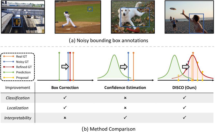
Figure 1: (a) Examples of noisy bounding box annotations. For simplicity, the noisy annotation for one object is presented per image. (b) Trait comparison of existing solutions and our DISCO. Their learning behaviors for one single border of bounding boxes are presented above as an illustration. Note that our DISCO can achieve improvement in all three aspects.

Due to the degenerated supervision introduced by noisy annotations, object detection with noisy bounding boxes remains a challenging problem. Obviously, such corrupt supervision signals could weaken the localization precision of object detectors. Besides, although the classification accuracy is less affected Liu et al. (2022), noisy bounding boxes do introduce biased category features during training, which reduces the generalization capability of classification. Notably, there is also a significant concern about the lack of interpretability for box predictions, especially considering the influence of noisy bounding box annotations.

Encountering the above challenges, existing solutions still exhibit drawbacks in this special setting (see Figure 1(b)). Several previous works are dedicated to correcting noisy bounding boxes Liu et al. (2022); Li et al. (2020a); Xu et al. (2021), aiming to mitigate the effect of noisy box annotations. However, their performance gains in classification and localization are constrained by heuristic box correction approaches, and the detector cannot identify which bounding boxes are inaccurately predicted. An alternative series of methods focus on equipping the model with the capability to estimate the confidence of predicted bounding boxes He et al. (2019); Li et al. (2020b); Choi et al. (2019), through which the detector can be more robust against noisy box annotations. Despite these efforts, it is unfortunate that the detector is still plagued by flawed supervision during training.

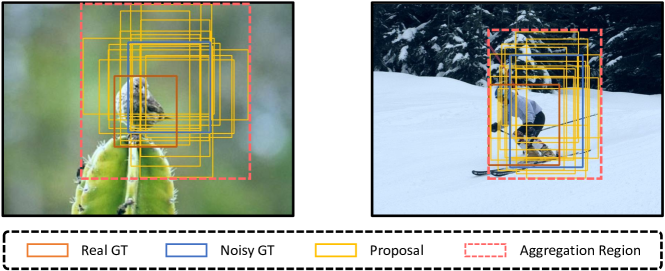
Figure 2: Examples of proposal aggregation in object detection with noisy bounding boxes. It can be observed that the real ground-truth is usually situated in the aggregation region of the proposals assigned to a noisy ground-truth.

Essentially, the corrupt supervision signals should be blamed for the above issues. In this work, we expect to answer the following question: How to properly calibrate the corrupt supervision signals? As shown in Figure 2, we observed that the real ground-truth is usually situated in the aggregation region of the proposals assigned to a noisy ground-truth, showing that the spatial distribution of proposals can act as a statistical prior for the potential locations of objects. Thus, we propose DIStribution-aware CalibratiOn (DISCO), which aims to model the spatial distribution of proposals for calibrating supervision signals (see Figure 1(b)). For each group of the assigned proposals, we perform spatial distribution modeling with a four-dimensional Gaussian distribution, statistically extracting potential locations of objects. Based on the modeled distribution, we develop three distribution-aware techniques to improve classification, localization, and interpretability, respectively: 1) Distribution-aware proposal augmentation (DA-Aug): Additional proposals are generated from the distribution to enrich category features in the representative locations, and then the proposal with the highest classification score is collected to boost classification performance; 2) Distribution-aware box refinement (DA-Ref): With a non-linear weighting strategy, noisy ground-truth is fused with the distribution into a refined ground-truth to achieve superior bounding box regression; 3) Distribution-aware confidence estimation (DA-Est): An extra estimator is integrated into the detection head, with the distribution variance elegantly acting as its supervision, to estimate the confidence of predicted bounding boxes. Without introducing complicated learnable modules, DISCO can attain state-of-the-art performance on large-scale noisy image datasets (i.e., Pascal VOC and MS-COCO), especially at high noise levels. Our main contributions are summarized as follows:

• Motivated by the observation about proposal aggregation, we propose an approach called DISCO to calibrate supervision signals with spatial distribution modeling.

• To improve classification, localization, and interpretability, we introduce three techniques (i.e., DA-Aug, DA-Ref, and DA-Est) to collaborate with the modeled distribution in a distribution-aware manner.

• Comprehensive experiments show that our DISCO can attain state-of-the-art performance in object detection with noisy bounding boxes and meanwhile achieve satisfactory interpretability for its predictions.

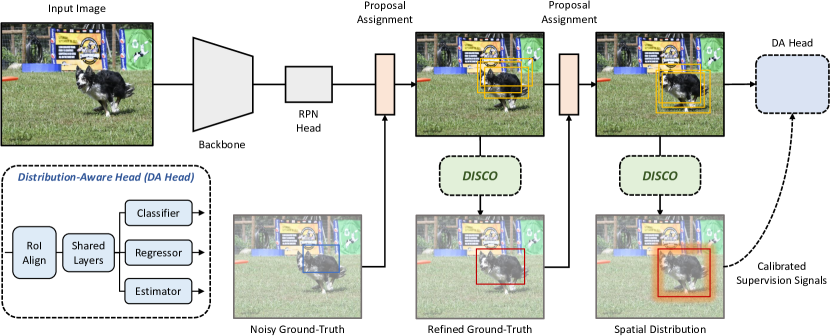
Figure 3: Training pipeline with our DISCO. DISCO is performed twice in a training iteration, the first time for proposal re-assignment to obtain better-matching proposals and the second time for producing calibrated supervision signals. In DISCO, spatial distribution modeling (Section 3.2) is performed firstly, followed by three distribution-aware techniques, i.e., DA-Aug (Section 3.3), DA-Ref (Section 3.4), and DA-Est (Section 3.5), to collaborate with the modeled distribution. Note that we additionally integrate an estimator into the vanilla detection head to construct the distribution-aware head (DA head) for the implementation of DISCO.

2 Related Works

2.1 Object Detection

The goal of object detection is to recognize what objects are present and where they are situated. Faster-RCNN Ren et al. (2015) is a classic detection framework with a two-stage strategy, and is widely adopted and improved in subsequent works Cai and Vasconcelos (2018); Pang et al. (2019); Sun et al. (2021). Moreover, RetinaNet Lin et al. (2017), YOLO Redmon et al. (2016), and CenterNet Zhou et al. (2019) delve into strengthening the performance of one-stage detectors. Recently, transformer-based detectors Carion et al. (2020); Zhu et al. (2020); Zhang et al. (2022) also attract the attention of the community, which conducts object detection in an end-to-end fashion. Training with accurate bounding box annotations, object detectors can achieve satisfactory and even remarkable performance. However, object detection with noisy bounding boxes remains an under-explored subproblem.

2.2 Object Detection with Noisy Annotations

Specifically, noisy annotations of an object detection dataset could compose of noisy category labels and noisy bounding boxes. Previous works Chadwick and Newman (2019); Li et al. (2020a); Xu et al. (2021) have made attempted to jointly tackle these two types of noisy annotations. Unlike this setting, we focus on training an object detector with noisy bounding boxes, since box noise is more common and challenging in realistic scenarios Liu et al. (2022). The state-of-the-art for this tough task is called OA-MIL Liu et al. (2022), which adopts a multi-instance learning (MIL) framework at the object level to correct bounding boxes. Besides, some approaches aiming to boost the robustness of detectors, such as KL Loss He et al. (2019), can also contribute to performance improvement in this task.

2.3 Weakly Supervised Object Detection

Weakly supervised object detection (WSOD) is also a relevant task, where only image-level labels can be accessed to train an object detector. The mainstream solution is to treat WSOD as a MIL problem Bilen and Vedaldi (2016); Wan et al. (2018); Chen et al. (2020); Tang et al. (2017), where each training image is constructed as a bag of instances. To handle the non-convex optimization of MIL, spatial regularization Diba et al. (2017); Wan et al. (2018), optimization strategy Tang et al. (2017); Wan et al. (2019), and context information Kantorov et al. (2016); Wei et al. (2018) are introduced to attain better convergence. Moreover, it is worth noting that SD-LocNet Zhang et al. (2019a) contributes a self-directed optimization strategy to handle object instances with noisy initial locations. Unfortunately, WSOD always results in relatively inaccurate box predictions due to the lack of fine-grained supervision. Effective methods for object detection with noisy bounding boxes can contribute to further refining these box predictions.

3 Methodology

3.1 Overview

In this work, we propose DISCO to calibrate the corrupt supervision signals caused by noisy bounding boxes in object detection. Essentially, DISCO is a training-time calibration approach designed for two-stage detectors. In a training iteration, DISCO is performed twice using the distribution-aware head (DA head) with the assigned proposals as input (see Figure 3). These two times of DISCO follow the same process and have only subtle differences for different purposes. The first time aims to yield a refined ground-truth for proposal re-assignment, by which better-matching proposals can be obtained. The second time aims to produce spatial distributions of proposals acting as superior supervision. In the following, we start by describing spatial distribution modeling in Section 3.2. Then, we will introduce three distribution-ware techniques (i.e., DA-Aug, DA-Ref, and DA-Est) in Section 3.3, 3.4 and 3.5, respectively, in which we will also detail the differences between these two times of DISCO.

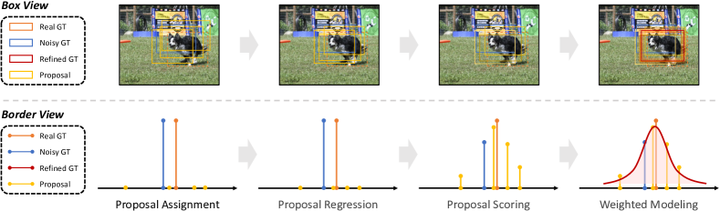
Figure 4: Illustration of spatial distribution modeling. For clarity, we present the process in the view of the whole bounding box and one single border. Note that the length of the vertical line indicates its weight. Here the refined ground-truth is essentially a spatial distribution.

3.2 Spatial Distribution Modeling

In DISCO, spatial distribution modeling is conducted for each group of the proposals assigned to a noisy/refined ground-truth (see Figure 4). Let $\mathbf{P}^{i}=[P^{i}_{1},P^{i}_{2},...,P^{i}_{N^{i}}]\in\mathbb{R}^{N^{i}\times 4}$ denotes the $i$-th group of the proposals, where $N^{i}$ is the number of the proposals in $\mathbf{P}^{i}$. Moreover, $\mathbf{P}^{i}$ is associated with a category indicator $l^{i}\in\{1,2,...,L\}$ where $L$ is the number of categories. Note that the noisy ground-truth is included in $\mathbf{P}^{i}$ as commonly done, and each proposal $P^{i}_{j}\in\mathbb{R}^{4}$ represents four coordinates of bounding boxes. First, the features of the proposals in $\mathbf{P}^{i}$ are extracted as

$$\mathbf{F}^{i}=\mathcal{F}(\mathbf{P}^{i},\mathbf{X})=[F^{i}_{1},F^{i}_{2},...,F^{i}_{N^{i}}]\in\mathbb{R}^{N^{i}\times D},$$ (1)

where $\mathcal{F}(\cdot,\cdot)$ is the joint operation of RoIAlign He et al. (2017) and two shared fully-connected layers, and $\mathbf{X}$ is the feature maps produced by the backbone. As a result, each proposal $P^{i}_{j}$ corresponds to a $D$-dimensional feature vector $F^{i}_{j}$. Then, we adopt the regressor $\mathcal{R}(\cdot)$ of the DA head to predict proposal offsets for further localization and update the features, which is formulated as

$$\mathbf{P}^{i*}=\operatorname{Trans}(\mathbf{P}^{i},\mathcal{R}(\mathbf{F}^{i}))\in\mathbb{R}^{N^{i}\times 4},$$ (2)

$$\mathbf{F}^{i*}=\mathcal{F}(\mathbf{P}^{i*},\mathbf{X})\in\mathbb{R}^{N^{i}\times D},$$ (3)

where $\operatorname{Trans(\cdot,\cdot)}$ is a function that translates predicted offsets to proposals Ren et al. (2015). Following Liu et al. (2022), we utilize classification scores to measure the possibilities of object locations. Therefore, the classifier $\mathcal{C}(\cdot)$ is used to score the proposals $\mathbf{F}^{i*}$, which is defined as

$$\mathbf{S}^{i}=\mathcal{C}(\mathbf{F}^{i*})\in\mathbb{R}^{N^{i}\times(L+1)},$$ (4)

$$S^{i}=\operatorname{LookUp}(\mathbf{S}^{i},l^{i})=[s^{i}_{1},s^{i}_{2},...,s^{i}_{N^{i}}]\in\mathbb{R}^{N^{i}},$$ (5)

where $\operatorname{LookUp}(\cdot,\cdot)$ is a look-up operation that extracts the $l^{i}$-th column from $\mathbf{S}^{i}$, and the resultant $S^{i}$ denotes the classification scores of the corresponding category. Subsequently, we utilize $S^{i}$ to produce the normalized weights $W^{i}$ for the proposals $\mathbf{F}^{i*}$, expressed as

$$W^{i}=\operatorname{Softmax}(S^{i},T)=[w^{i}_{1},w^{i}_{2},...,w^{i}_{N^{i}}]\in\mathbb{R}^{N^{i}},$$ (6)

where $\operatorname{Softmax}(\cdot,\cdot)$ is the Softmax function to obtain normalized weights (sum up to $1$) and $T$ is the temperature coefficient Hinton et al. (2015) to control its sharpness. Finally, we model the spatial distribution of $\mathbf{P}^{i*}$ as a four-dimensional Gaussian distribution by directly calculating its parameters (i.e., mean $\mu^{i}$ and standard deviation $\sigma^{i}$) in a weighting manner, which can be formulated as

$$\mu^{i}=\sum_{j=1}^{N^{i}}w^{i}_{j}*P^{i*}_{j}\in\mathbb{R}^{4},$$ (7)

$$\sigma^{i}=\sqrt{\sum_{j=1}^{N^{i}}w^{i}_{j}*(P^{i}_{j}-\mu^{i})^{2}}\in\mathbb{R}^{4},$$ (8)

where we assume that each dimension of this Gaussian distribution is uncorrelated so that its standard deviation can be formulated as a four-dimensional vector. Note that $w^{i}_{j}$ is already normalized so dividing the sum is unnecessary. This assumption simplifies the modeling problem, makes the method more computationally efficient, and is not detrimental to performance. Therefore, it has been widely adopted in previous works, such as KL Loss He et al. (2019), GFL Li et al. (2020b), and Gaussian YOLOv3 Choi et al. (2019).

3.3 Distribution-Aware Proposal Augmentation

Instead of using heuristic approaches such as selective search Uijlings et al. (2013) and edge box Zitnick and Dollár (2014), we propose to augment proposals with the modeled distribution, aiming to statistically cover more potential locations of objects. Firstly, we create a Guassian noise matrix $\mathbf{G}\in\mathbb{R}^{N^{\prime}\times 4}$ whose each element is sampled from $\mathcal{N}(0,1)$ to ensure randomness. Here $N^{\prime}$ is a hyperparameter that indicates the number of augmented proposals. Then, augmented proposals $\mathbf{P}^{i\prime}$ can be generated by

$$\mathbf{P}^{i\prime}=\mu^{i}+\mathbf{G}\odot\sigma^{i}=[P^{i\prime}_{1},P^{i\prime}_{2},...,P^{i\prime}_{N^{\prime}}]\in\mathbb{R}^{N^{\prime}\times 4},$$ (9)

where $\odot$ denotes element-wise multiplication and the operations here are all conducted in a broadcasting fashion. Following Equation 4 and 5, its classification scores $S^{i\prime}$ can be obtained. Subsequently, we incorporate the augmented proposals $\mathbf{P}^{i\prime}$ into $\mathbf{P}^{i}$, expressed as

$$\mathbf{P}^{i*}\leftarrow\mathbf{P}^{i*}\oplus\mathbf{P}^{i\prime}\in\mathbb{R}^{(N^{i}+N^{\prime})\times 4},$$ (10)

$$S^{i}\leftarrow S^{i}\oplus S^{i\prime}\in\mathbb{R}^{N^{i}+N^{\prime}},$$ (11)

where $\oplus$ indicates proposal-wise concatenation. To boost classification performance, the proposals with the highest classification score, which could contain representative category features, are collected to form a loss term for classification, formulated as

$$s^{i}_{\star}=\max_{j}s^{i}_{j},\quad j=1,2,...,(N^{i}+N^{\prime}),$$ (12)

$$\mathcal{L}_{\text{Aug}}=-\frac{1}{M}\sum_{i=1}^{M}\log(s^{i}_{\star}),$$ (13)

where $M$ is the number of proposal groups in a batch. Note that $\mathcal{L}_{\text{Aug}}$ does not be computed in the first-time DISCO. Finally, after proposal augmentation, we follow Equation 7 and 8 to model the spatial distribution of $\mathbf{P}^{i*}$ once again for a better representation of these proposals.

Method	VOC				COCO
	Noise Level				20% Noise Level						40% Noise Level    [t]
	10%	20%	30%	40%	AP	$\text{AP}_{50}$	$\text{AP}_{75}$	$\text{AP}_{\text{S}}$	$\text{AP}_{\text{M}}$	$\text{AP}_{\text{L}}$	AP	$\text{AP}_{50}$	$\text{AP}_{75}$	$\text{AP}_{\text{S}}$	$\text{AP}_{\text{M}}$	$\text{AP}_{\text{L}}$ [b]
Clean-FasterRCNN	77.2	77.2	77.2	77.2	37.9	58.1	40.9	21.6	41.6	48.7	37.9	58.1	40.9	21.6	41.6	48.7 [t]
FasterRCNN	76.3	71.2	60.1	42.5	30.4	54.3	31.4	17.4	33.9	38.7	10.3	28.9	3.3	5.7	11.8	15.1 [t]
RetinaNet	71.5	67.5	57.9	45.0	30.0	53.1	30.8	17.9	33.7	38.2	13.3	33.6	5.7	8.4	15.9	18.0
Co-teaching	75.4	70.6	60.9	43.7	30.5	54.9	30.5	17.3	34.0	39.1	11.5	31.4	4.2	6.4	13.1	16.4
SD-LocNet	75.7	71.5	60.8	43.9	30.0	54.5	30.3	17.5	33.6	38.7	11.3	30.3	4.3	6.0	12.7	16.6
FreeAnchor	73.0	67.5	56.2	41.6	28.6	53.1	28.5	16.6	32.2	37.0	10.4	28.9	3.3	5.8	12.1	14.9
KL Loss	75.8	72.7	64.6	48.6	31.0	54.3	32.4	18.0	34.9	39.5	12.1	36.7	3.7	6.2	13.0	17.4
OA-MIL	77.4	74.3	70.6	63.8	32.1	55.3	33.2	18.1	35.8	41.6	18.6	42.6	12.9	9.2	19.0	26.5
DISCO (Ours)	77.5	75.3	72.1	68.7	32.3	54.7	34.5	18.7	35.8	41.2	21.2	45.7	16.9	11.4	24.7	27.8 [b]

Table 1: Benchmark results on VOC and COCO. Note that Clean-FasterRCNN is trained with clean annotations for reference. In noisy settings, the best results are marked in bold. Our DISCO can achieve state-of-the-art performance especially at high noise levels.

Method	Noise Level	AP	$\text{AP}_{50}$	$\text{AP}_{75}$	$\text{AP}_{\text{S}}$	$\text{AP}_{\text{M}}$	$\text{AP}_{\text{L}}$
OA-MIL	10%	35.1	57.2	37.9	20.5	38.5	44.9 [t]
DISCO (Ours)		36.1	57.3	39.4	20.8	39.5	45.7 [b]
OA-MIL	30%	24.6	49.1	21.9	13.8	27.5	32.7 [t]
DISCO (Ours)		26.4	49.8	25.3	14.2	29.7	34.2 [b]

Table 2: Experimental results on COCO at 10% and 30% noise levels. Our DISCO can still outperform OA-MIL and achieve state-of-the-art performance in additional noisy settings.

3.4 Distribution-Aware Box Refinement

As we mentioned before, the modeled spatial distribution can be considered as a statistical prior for the potential locations of objects. Therefore, it can act as guidance for noisy bounding box refinement. First, we treat $\mu^{i}$ as a proposal, extract its feature with $\mathcal{F}(\cdot,\cdot)$, and adopt the classifier $\mathcal{C}(\cdot)$ to obtain its classification score $s^{i}_{\mu}$. Then, the noisy bounding box $B^{i}$ is refined as $B^{i\prime}$ by a fusion strategy as

$$B^{i\prime}=\phi(s^{i}_{\mu})\cdot\mu^{i}+(1-\phi(s^{i}_{\mu}))\cdot B^{i},$$ (14)

where $\phi(\cdot)$ is a non-linear weighting function following Liu et al. (2022). To stabilize the early stage of training, the fusion strategy is conditional on the classification score $s^{i}_{\mu}$, and thus the $\phi(\cdot)$ is defined as

$$\phi(s^{i}_{\mu})=\min((s^{i}_{\mu})^{\alpha},\beta),$$ (15)

where $\alpha$ and $\beta$ are two hyperparameters. It means that the higher $s^{i}_{\mu}$ is, the more the model would reply on $\mu^{i}$. Finally, the refined $B^{i\prime}$ is used as supervision for the original proposals $\mathbf{P}^{i}$ to compute regression loss as

$$\mathcal{L}_{\text{reg}}=\frac{1}{M}\sum_{i=1}^{M}\frac{1}{N^{i}}\sum_{j=1}^{N^{i}}\operatorname{Dist}(P^{i}_{j},B^{i\prime}),$$ (16)

where $\operatorname{Dist}(\cdot,\cdot)$ is a predefined distance function for two bounding boxes Ren et al. (2015). It is worth noting that the first-time DISCO is ended with Equation 14 to obtain the refined ground-truth $B^{i\prime}$ for proposal re-assignment.

3.5 Distribution-Aware Confidence Estimation

To estimate the confidence of predicted bounding boxes, we integrate an estimator $\mathcal{E}(\cdot)$ into the DA head. Note that $\mathcal{E}(\cdot)$ comprises only one fully-connected layer. As excepted, the confidence $\mathbf{V}^{i}$ for the proposals $\mathbf{P}^{i}$ can be produced as

$$\mathbf{V}^{i}=\mathcal{E}(\mathbf{F}^{i})=[V^{i}_{1},V^{i}_{2},...,V^{i}_{N^{i}}]\in\mathbb{R}^{N^{i}\times 4}.$$ (17)

In the modeled spatial distribution, the variance (or standard deviation) can measure the border-wise variability of the potential locations of objects. Therefore, the distribution variance can be elegantly adopted as the supervision of the estimator $\mathcal{E}(\cdot)$. The loss for training $\mathcal{E}(\cdot)$ is formulated as

$$\mathcal{L}_{\text{Est}}=\frac{1}{M}\sum_{i=1}^{M}\frac{1}{N^{i}}\sum_{j=1}^{N^{i}}\|V^{i}_{j}-(\sigma^{i})^{2}\|_{1}.$$ (18)

Different from He et al. (2019), we train the estimator with direct supervision of variance rather than implicit supervision of bounding boxes. Then, the estimated confidence (i.e., predicted variance) is used in Softer-NMS He et al. (2019) for a better inference-time process. Finally, the overall loss function is formed as

$$\mathcal{L}_{\text{All}}=\mathcal{L}_{\text{Cls}}+\mathcal{L}_{\text{Reg}}+\gamma\mathcal{L}_{\text{Est}}+\lambda\mathcal{L}_{\text{Aug}},$$ (19)

where $\gamma$ and $\lambda$ is two hyperparameters to down-weight $\mathcal{L}_{\text{Est}}$ and $\mathcal{L}_{\text{Aug}}$ respectively, and $\mathcal{L}_{\text{Cls}}$ is a cross-entropy classification loss for the original proposals $\mathbf{P}^{i}$ Ren et al. (2015).

Method	VOC	COCO
	$\text{AP}_{50}$	AP	$\text{AP}_{50}$	$\text{AP}_{75}$	$\text{AP}_{\text{S}}$	$\text{AP}_{\text{M}}$	$\text{AP}_{\text{L}}$
OA-MIL	77.1	37.0	57.9	40.3	21.8	40.6	47.6 [t]
DISCO (Ours)	78.0	38.0	57.9	41.9	21.9	41.4	48.5 [b]

Table 3: Experimental results on the original VOC and COCO. Unlike OA-MIL, Our DISCO can still provide performance improvement even without manually introducing noise.

4 Experiments

4.1 Experimental Setup

Datasets.

Two large-scale image datasets are adopted in our experiments, including Pascal VOC 2007 Everingham et al. (2010) and MS-COCO 2017 Lin et al. (2014). Pascal VOC 2007 (VOC) is a standard dataset for object detection, consisting of $9,963$ images with $24,640$ box annotations. MS-COCO 2017 (COCO) is also a popular object detection benchmark, containing $328,000$ images of generic objects. Following Liu et al. (2022), noisy box annotations are simulated by perturbing clean ones at various noise levels which are set to $\{10\%,20\%,30\%,40\%\}$ for VOC and $\{20\%,40\%\}$ for COCO (see more details in Appendix A.1).

Component			Category																				All [t]
DA-Aug	DA-Ref	DA-Est	Aero	Bicy	Bird	Boat	Bot	Bus	Car	Cat	Cha	Cow	Dtab	Dog	Hors	Mbik	Pers	Plnt	She	Sofa	Trai	Tv	[b]
$\checkmark$			49.4	69.5	47.4	32.1	35.2	62.3	64.1	60.3	31.9	55.1	41.5	61.8	54.3	56.8	58.7	22.5	48.6	49.7	49.8	51.3	50.1 [t]
	$\checkmark$		56.0	70.6	56.0	38.5	33.0	64.7	74.8	77.4	32.2	58.5	42.4	72.1	65.6	64.8	62.5	23.4	51.2	51.5	65.7	50.5	55.6
	$\checkmark$	$\checkmark$	61.2	74.4	59.7	43.1	37.0	69.4	75.2	73.3	34.8	64.1	54.5	74.1	71.7	66.0	66.7	28.7	54.1	55.4	70.5	60.2	59.7
$\checkmark$	$\checkmark$		69.9	77.1	68.2	47.2	49.9	70.9	80.6	80.8	43.0	76.4	60.0	82.6	81.0	74.4	73.4	39.2	62.7	64.3	67.9	68.6	66.9
$\checkmark$	$\checkmark$	$\checkmark$	71.5	76.9	71.5	45.6	52.2	76.1	81.2	83.2	43.4	79.8	60.3	81.5	82.9	75.4	73.6	40.6	64.4	68.2	76.8	70.0	68.7 [b]

Table 4: Ablation studies of component effectiveness. Note that per-category performance is reported for a detailed comparison. The proposed components (i.e., three distribute-aware techniques) of our DISCO can all contribute to performance improvement.

Hyper.	Value	$\text{AP}_{50}$
$T$	0.01	68.6
	0.1	68.7
	0.2	67.8

Hyper.	Value	$\text{AP}_{50}$
$\alpha$	3	68.3
	5	68.7
	7	68.2

Hyper.	Value	$\text{AP}_{50}$
$\beta$	0.7	68.1
	0.8	68.7
	0.9	67.3

Table 5: Ablation studies of hyperparameter sensitivity. DISCO can still achieve relatively stable performance when these hyperparameters vary within a moderate range.

Implementation Details.

Following Liu et al. (2022), we implement our method on FasterRCNN Ren et al. (2015) with ResNet-50 He et al. (2016) as the backbone. The idea of DISCO can be easily generalized to other frameworks and we choose to perform our experiments with FasterRCNN as it is widely adopted Kaur and Singh (2023). As a common practice, the model is trained with the “$1\times$” schedule Girshick et al. (2018). Hyperparameter selections of our method are detailed in Appendix A.2. Notably, all other training configurations are aligned with Liu et al. (2022) to ensure fairness.

Evaluation Metrics.

As commonly done, mean average precision (mAP@$.5$) and mAP@$[.5,95]$ are used for VOC and COCO respectively. Specifically, we report $\text{AP}_{50}$ for VOC and $\{\text{AP},\text{AP}_{50},\text{AP}_{75},\text{AP}_{S},\text{AP}_{M},\text{AP}_{L}\}$ for COCO.

4.2 Results and Discussions

We compare DISCO with the state-of-the-art methods of this task, including FasterRCNN Ren et al. (2015), Co-teaching Han et al. (2018), SD-LocNet Zhang et al. (2019a), KL Loss He et al. (2019), and OA-MIL Liu et al. (2022). Besides, the results of two one-stage methods are presented for a further comparison, including RetinaNet Lin et al. (2017) and FreeAnchor Zhang et al. (2019b). For reference, we also report the result of Clean-FasterRCNN, which is trained with clean annotations under the same setup.

Benchmark Results.

Benchmark results are reported in Table 1. It can be observed that noisy bounding box annotations significantly reduce the performance of vanilla object detectors like FasterRCNN, especially at high box noise levels. Moreover, Co-teaching and SD-LocNet can only marginally improve detection performance, showing that small-loss sample selection and sample weight assignment are not decent solutions for handling noisy bounding boxes. Besides, even with better label assignment, FreeAnchor still underperforms in such a challenging task. It is worth noting that KL Loss is a competitive method that also improves the interpretability of detectors. Moreover, OA-MIL adopts a MIL-based training strategy by iteratively constructing object-level bags, attaining better detection performance than the aforementioned methods. As shown in Table 1, our DISCO, which aims to calibrate the corrupt supervision signals caused by noisy bounding boxes, achieves state-of-the-art performance on these two benchmarks. Notably, it can significantly outperform the existing methods at high noise levels (i.e., $30\%$ and $40\%$), showing that our method is more robust to noisy bounding boxes. Specifically, compared with OA-MIL, DISCO attains $+1.5\text{AP}_{50}$ and $+4.9\text{AP}_{50}$ improvement on VOC at the $30\%$ and $40\%$ noise levels respectively. DISCO can also achieve $+2.6\text{AP}$, $+3.1\text{AP}_{50}$, and $+4.0\text{AP}_{75}$ improvement on COCO at the $40\%$ noise level.

Additional Evaluations.

To further demonstrate the effectiveness of our DISCO, We compare it with OA-MIL in more settings other than those included in Liu et al. (2022). The additional evaluations include two aspects: 1) Performance on COCO at $10\%$ and $30\%$ noise levels: Compared to OA-MIL, Our DISCO can still achieve state-of-the-art performance in additional noisy settings on COCO (see Figure 2), suggesting its flexibility for various noise levels; 2) Performance on the original VOC and COCO (i.e., the noise level is set to $0\%$): Without manually introducing noise, DISCO can still provide performance improvement on original datasets (see Figure 3), especially on VOC, showing that it has the potential to be generalized to real-world noisy scenarios.

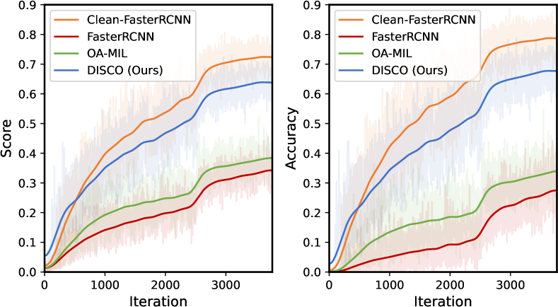
Figure 5: Illustration of classification performance improvement. Left: Average classification scores of the positive proposals for corresponding categories. Right: Classification accuracy of the positive proposals. Compared to OA-MIL, DISCO can provide superior improvement for classification, which even approaches the results of training with clean annotations.

4.3 Ablation Studies

We conduct comprehensive ablation studies including component effectiveness and hyperparameter sensitivity to further verify DISCO’s performance. Due to space limitation, more ablation studies (e.g., backbone compatibility) are provided in Appendix B. Unless otherwise specified, the following experiments are all based on VOC at the $40\%$ noise level.

Component Effectiveness.

To investigate the effectiveness of three key techniques in DISCO (i.e., DA-Aug, DA-Ref, and DA-Est), we gradually integrate them into training. Note that the implementation of DA-Est is heavily based on DA-Ref thus it cannot be adopted independently. The experimental results are reported in Table 4, where we also list per-category performance for a detailed comparison. Notably, using only DA-Aug or DA-Ref can considerably contribute to performance improvement. DA-Ref seems to be more effective since it comes with refined ground-truths for better localization. Moreover, its detection performance can be further boosted when collaborating with DA-Aug or DA-Est. It is also worth noting that DA-Est can achieve $+4.1\text{AP}_{50}$ improvement by enhancing the robustness of detectors. Adopting all three techniques, our DISCO can attain superior detection performance in almost all categories, demonstrating the performance improvement of these components.

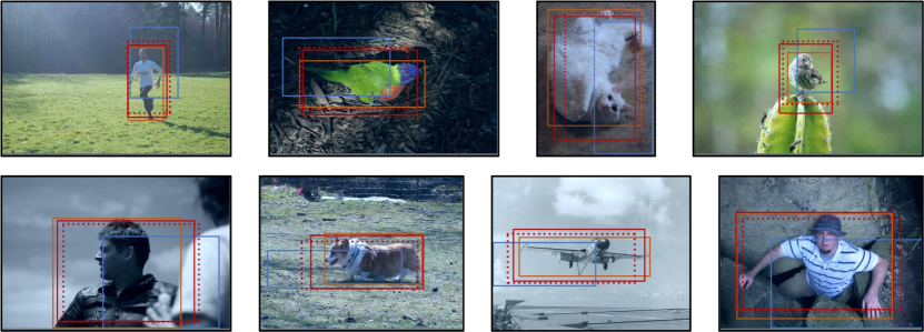
Figure 6: Qualitative results of box refinement in DISCO. Real ground-truths and noisy ground-truths are marked in orange and blue. Refined bounding boxes produced by the first-/second-time DISCO are indicated in dotted/solid red. The first-time refined boxes can cover the objects more tightly than noisy ground-truths, and the second-time refinement can further contribute to more precise ones.

Hyperparameter Sensitivity.

Here we evaluate the sensitivity of $T$ of Equation 6 and $\alpha,\beta$ of Equation 15. The evaluations of other hyperparameters are provided in Appendix B.2. Note that we choose some moderate values rather than extreme ones to reasonably evaluate the sensitivity. As shown in Table 5, the temperature coefficient $T$ is relatively robust when set to 0.01 or 0.2. Tuning $T$ to a proper value can contribute to better performance. Moreover, the hyperparameters regulate the fusion of two bounding boxes (i.e., $\alpha$ and $\beta$) is also insensitive when varying within a moderate range, showing the effectiveness of our method.

4.4 Further Analysis

In this subsection, additional evidence and discussion are provided to further analyze the advantages of DISCO in classification, localization, and interpretability, respectively. Unless otherwise specified, the following experiments are all based on VOC at the $40\%$ noise level.

Classification Performance Improvement.

DA-Aug is used to generate proposals in the potential locations of objects for obtaining representative category features, by which classification performance can be boosted. The evidence is provided in Figure 5. It shows that noisy bounding box annotations can badly reduce the classification scores and the accuracy of foreground features. Notably, OA-MIL can also enhance classification performance. More importantly, DISCO provides superior improvement for classification, which even approaches the results of training with clean annotations.

Box Refinement for Better Localization.

To improve the localization capability of detectors, DA-Ref utilizes the modeled distributions of proposals for noisy box refinement (see Figure 6). Note that DISCO is performed twice in a training iteration and thus there are two successive refined boxes, where the first one is for proposal re-assignment and the second one acts as the supervision for regression. Since box refinement is very challenging when given only noisy ground-truths, it is natural that refined ones may be not exactly identical to real ones. Even so, the refined boxes can cover the objects more tightly than noisy ground-truths. Furthermore, the second-time refinement contributes to more precise ones, showing the effectiveness of our refinement strategy.

Interpretability with Confidence Estimation.

We introduce interpretability into box predictions in DISCO, aiming to enhance the robustness of detectors. The term “interpretability” is used to convey that our box predictions are interpretable, which is also adopted in He et al. (2019). This is implemented by estimating the confidence of each border of the predicted bounding boxes with the variance of the modeled distribution as its supervision. For an intuitive understanding, some qualitative results are represented in Figure 7. For a predicted border that deviates largely from the real one, DISCO could estimate a relatively large variance, indicating low confidence for this prediction. Such a crucial property enhances the practicability of DISCO in realistic scenarios.

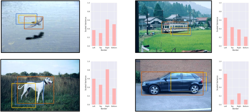
Figure 7: Qualitative results of interpretability in DISCO. We randomly choose an assigned proposal (yellow) per image to report its estimated variances. Real ground-truths and noisy ground-truths are marked in orange and blue. Note that the variance is scaled by the width and height for clarity. With the proposed DA-Est, DISCO can estimate reasonable variances for each border of box prediction.

5 Conclusions

In this paper, we focus on an under-explored and challenging problem termed object detection with noisy bounding boxes. Motivated by the observation about proposal aggregation, we propose DISCO to calibrate the corrupt supervision signals. Spatial distribution modeling is performed and then three distribution-aware techniques (i.e., DA-Aug, DA-Ref, and DA-Est) are adopted successively. Experiments show that our DISCO can achieve state-of-the-art performance. We believe that DISCO can serve as a stronger baseline for this task and expect it can motivate more future works in the field of object detection and learning with noisy labels.

Appendix

Appendix A Details of the Experimental Setup

A.1 Noise Simulation

Following Liu et al. [2022], clean annotations are perturbed to simulate noisy bounding box annotations in our experiments, which is performed once for each dataset. Specifically, let $c_{\text{x}},c_{\text{y}},w,h$ represent the central x-axis coordinate, central y-axis coordinate, width, and height of a clean bounding box, respectively. We simulate a noisy bounding box by randomly shifting and scaling a clean one, which can be formulated as

$$\left\{\begin{aligned} &\hat{c}_{\text{x}}=c_{\text{x}}+\Delta_{\text{x}}\cdot w,\ &\hat{c}_{\text{y}}=c_{\text{y}}+\Delta_{\text{y}}\cdot h,\\ &\hat{w}=(1+\Delta_{\text{w}})\cdot w,\ &\hat{h}=(1+\Delta_{\text{h}})\cdot h,\end{aligned}\right.$$ (20)

where $\Delta_{\text{x}}$, $\Delta_{\text{y}}$, $\Delta_{\text{w}}$, and $\Delta_{\text{h}}$ obey the uniform distribution $U(-n,n)$ and $n$ is the noise level. For example, when $n$ is set to $40\%$, $\Delta_{\text{x}}$, $\Delta_{\text{y}}$, $\Delta_{\text{w}}$, and $\Delta_{\text{h}}$ would ranges from $-0.4$ to $0.4$. Note that Equation 20 is conducted on each bounding box of the training set. Such a noise simulation can guarantee access to real ground-truths for analyzing training behaviors and evaluating the performance of box refinement.

A.2 Hyperparameter Selections

There are six hyperparameters in DISCO, including the temperature coefficient $T$, the augmented proposal number $N^{\prime}$, two box fusion hyperparameters $\alpha$ and $\beta$, and two loss weights $\gamma$ and $\lambda$. As there are no additional validation sets available, we tuned these hyperparameters based on the performance on the training set with clean annotations, which can also avoid the leakage of test data. For the sake of simplicity, we empirically fix $N^{\prime}$ and $\gamma$ to $10$ and $0.3$, and then tuning $T\in[0.01,0.2]$, $\alpha\in[3,10]$, $\beta\in[0.7,0.9]$, and $\lambda\in[0.01,0.2]$. To ensure reproducibility, the selected hyperparameters for all settings are reported in Table 6. Notably, we have just roughly tuned these hyperparameters by selecting some regular values, thus the performance of our method in Table 1 has the potential to be better.

Appendix B More Ablation Studies

In this section, we conduct more ablation studies to further verify the effectiveness of the proposed DISCO. These ablation studies contain backbone compatibility, sensitivity analysis of other hyperparameters, and the execution number of DISCO. Unless otherwise specified, the following experiments are all based on VOC at the $40\%$ noise level.

B.1 Backbone Compatibility

As mentioned in Section 4.1, following Liu et al. [2022], the benchmark experiments are performed with ResNet-50 He et al. [2016] as the backbone. To further demonstrate the superior performance of our method, we conduct an additional experiment based on different backbones. Specifically, in this experiment, DISCO is compared to OA-MIL on COCO at the $40\%$ noise level with the backbone set to ResNet-101 He et al. [2016] and Swin-T Liu et al. [2021], and other experiment setups remain the same. In this way, we aim to evaluate the performance of our DISCO for a large-scale dataset when it is equipped with an advanced backbone. The experimental results are reported in Table 7. For ResNet-101, it can be observed that our DISCO can further improve performance and still achieve state-of-the-art results. For Swin-T, although the noisy setting and training configurations may not be suitable for this backbone, compared to OA-MIL, our DISCO can still attain superior detection performance.

Dataset	Noise Level	Hyperparameter     [t]
		$T$	$N^{\prime}$	$\alpha$	$\beta$	$\gamma$	$\lambda$ [b]
VOC	10%	0.05	10	10	0.7	0.3	0.05 [t]
	20%	0.05	10	10	0.7	0.3	0.05
	30%	0.1	10	10	0.8	0.3	0.1
	40%	0.1	10	5	0.8	0.3	0.1 [b]
COCO	20%	0.01	10	10	0.7	0.3	0.01 [t]
	40%	0.1	10	5	0.8	0.3	0.1 [b]

Table 6: Hyperparameter selections. We report the hyperparameters for all settings to ensure reproducibility.

Method	Backbone	AP	$\text{AP}_{50}$	$\text{AP}_{75}$	$\text{AP}_{\text{S}}$	$\text{AP}_{\text{M}}$	$\text{AP}_{\text{L}}$
OA-MIL	ResNet-101	19.3	44.1	13.1	9.3	20.8	27.8 [t]
DISCO (Ours)		22.7	47.6	18.4	12.9	26.6	29.8 [b]
OA-MIL	Swin-T	15.5	37.0	9.7	7.7	15.7	23.1 [t]
DISCO (Ours)		18.0	42.1	12.0	10.3	20.6	24.0 [b]

Table 7: Ablation studies of backbone compatibility. The experiment is conducted on COCO at 40% noise level with ResNet-101 and Swin-T. DISCO can still outperform OA-MIL when equipped with different backbones.

B.2 Other Hyperparameter Sensitivity

We perform sensitivity analysis for other hyperparameters, including $N^{\prime}$ of Equation 9 and $\gamma,\lambda$ of Equation 19. Note that we choose some moderate values rather than extreme ones to reasonably evaluate the sensitivity for each hyperparameter. The experimental results are reported in Table 8. It can be observed that the augmented proposal number $N^{\prime}$ is insensitive when varying from $5$ to $20$. This is the reason why we empirically fix $N^{\prime}$ to $10$ for all settings. Besides, two loss weights $\gamma,\lambda$ also remain insensitive while $\lambda$ is relatively crucial. This is because it controls the strength of an extra classification loss term, directly affecting classification accuracy.

B.3 Execution Number of DISCO

In this work, DISCO is performed twice in a training iteration, where the first time is for proposal re-assignment and the second time is for obtaining better supervision. We compare such an execution strategy with two other options: 1) The execution number of DISCO is set to $1$: proposal re-assignment is removed and the only one time of DISCO is for obtaining better supervision; 2) The execution number of DISCO is set to $3$: the first two times are for proposal re-assignment and the third time is for obtaining better supervision. As shown in Table 9, more execution numbers of DISCO do not contribute to better detection performance. This is because such an improper strategy could result in excessive box refinement and thus influence the learning stability of detectors. Moreover, it also can be observed that our execution strategy can achieve superior performance.

Hyper.	Value	$\text{AP}_{50}$
$N^{\prime}$	5	68.5 [t]
	10	68.7
	20	68.6 [b]

Hyper.	Value	$\text{AP}_{50}$
$\gamma$	0.1	68.3 [t]
	0.3	68.7
	0.5	68.4 [b]

Hyper.	Value	$\text{AP}_{50}$
$\lambda$	0.05	67.9 [t]
	0.1	68.7
	0.15	67.4 [b]

Table 8: Ablation studies of hyperparameter sensitivity. DISCO can still achieve relatively stable performance when these hyperparameters vary within a moderate range.

Execution Number of DISCO	$\text{AP}_{50}$
1	68.1 [t]
2	68.7
3	67.9 [b]

Table 9: Ablation studies of the execution number of DISCO. Our execution strategy can achieve superior performance.

Appendix C More Qualitative Results

C.1 Box Refinement

As an extension to Figure 6, we present more qualitative results of box refinement in DISCO (see Figure 8), which shows that DISCO can attain tighter bounding boxes than noisy ground-truths. As shown in Figure 8, it is worth noting that DISCO can achieve consistent refinement of bounding boxes for different objects varying in size.

C.2 Interpretability

In Figure 9, more qualitative results of interpretability in DISCO are provided to demonstrate such a characteristic of our method. As shown in Figure 9, when trained with DISCO, the detector can output a reasonable variance as the confidence for each border of predicted bounding boxes, which shows that the detector is capable of realizing which border may be inaccurately predicted.

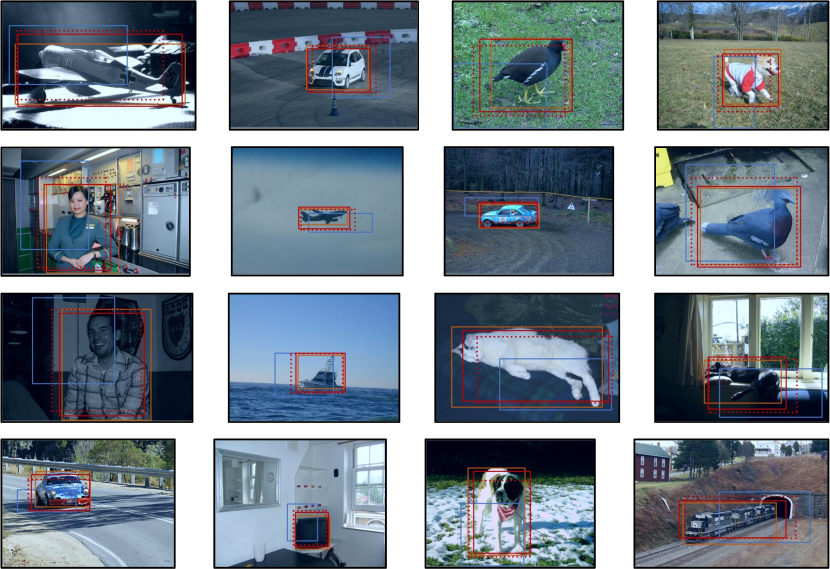
Figure 8: Qualitative results of box refinement in DISCO. Real ground-truths and noisy ground-truths are marked in orange and blue. Refined bounding boxes produced by the first-/second-time DISCO are indicated in dotted/solid red. The first-time refined boxes can cover the objects more tightly than noisy ground-truths, and the second-time refinement can further contribute to more precise ones.

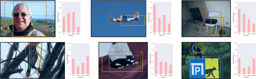
Figure 9: Qualitative results of interpretability in DISCO. We randomly choose an assigned proposal (yellow) per image to report its estimated variances. Real ground-truths and noisy ground-truths are marked in orange and blue. Note that the variance is scaled by the width and height for clarity. With the proposed DA-Est, DISCO can estimate reasonable variances for each border of box prediction.

References

- Bilen and Vedaldi [2016] Hakan Bilen and Andrea Vedaldi. Weakly supervised deep detection networks. In Proceedings of the IEEE conference on computer vision and pattern recognition, pages 2846–2854, 2016.
- Cai and Vasconcelos [2018] Zhaowei Cai and Nuno Vasconcelos. Cascade r-cnn: Delving into high quality object detection. In Proceedings of the IEEE conference on computer vision and pattern recognition, pages 6154–6162, 2018.
- Carion et al. [2020] Nicolas Carion, Francisco Massa, Gabriel Synnaeve, Nicolas Usunier, Alexander Kirillov, and Sergey Zagoruyko. End-to-end object detection with transformers. In European conference on computer vision, pages 213–229. Springer, 2020.
- Chadwick and Newman [2019] Simon Chadwick and Paul Newman. Training object detectors with noisy data. In 2019 IEEE Intelligent Vehicles Symposium (IV), pages 1319–1325. IEEE, 2019.
- Chai et al. [2023] Zhizhong Chai, Luyang Luo, Huangjing Lin, Pheng-Ann Heng, and Hao Chen. Deep omni-supervised learning for rib fracture detection from chest radiology images. arXiv preprint arXiv:2306.13301, 2023.
- Chen et al. [2020] Ze Chen, Zhihang Fu, Rongxin Jiang, Yaowu Chen, and Xian-Sheng Hua. Slv: Spatial likelihood voting for weakly supervised object detection. In Proceedings of the IEEE/CVF Conference on Computer Vision and Pattern Recognition, pages 12995–13004, 2020.
- Choi et al. [2019] Jiwoong Choi, Dayoung Chun, Hyun Kim, and Hyuk-Jae Lee. Gaussian yolov3: An accurate and fast object detector using localization uncertainty for autonomous driving. In Proceedings of the IEEE/CVF International conference on computer vision, pages 502–511, 2019.
- Diba et al. [2017] Ali Diba, Vivek Sharma, Ali Pazandeh, Hamed Pirsiavash, and Luc Van Gool. Weakly supervised cascaded convolutional networks. In Proceedings of the IEEE conference on computer vision and pattern recognition, pages 914–922, 2017.
- Everingham et al. [2010] Mark Everingham, Luc Van Gool, Christopher KI Williams, John Winn, and Andrew Zisserman. The pascal visual object classes (voc) challenge. International journal of computer vision, 88:303–338, 2010.
- Girshick et al. [2018] Ross Girshick, Ilija Radosavovic, Georgia Gkioxari, Piotr Dollár, and Kaiming He. Detectron, 2018.
- Han et al. [2018] Bo Han, Quanming Yao, Xingrui Yu, Gang Niu, Miao Xu, Weihua Hu, Ivor Tsang, and Masashi Sugiyama. Co-teaching: Robust training of deep neural networks with extremely noisy labels. Advances in neural information processing systems, 31, 2018.
- He et al. [2016] Kaiming He, Xiangyu Zhang, Shaoqing Ren, and Jian Sun. Deep residual learning for image recognition. In Proceedings of the IEEE conference on computer vision and pattern recognition, pages 770–778, 2016.
- He et al. [2017] Kaiming He, Georgia Gkioxari, Piotr Dollár, and Ross Girshick. Mask r-cnn. In Proceedings of the IEEE international conference on computer vision, pages 2961–2969, 2017.
- He et al. [2019] Yihui He, Chenchen Zhu, Jianren Wang, Marios Savvides, and Xiangyu Zhang. Bounding box regression with uncertainty for accurate object detection. In Proceedings of the ieee/cvf conference on computer vision and pattern recognition, pages 2888–2897, 2019.
- Hinton et al. [2015] Geoffrey Hinton, Oriol Vinyals, and Jeff Dean. Distilling the knowledge in a neural network. arXiv preprint arXiv:1503.02531, 2015.
- Kantorov et al. [2016] Vadim Kantorov, Maxime Oquab, Minsu Cho, and Ivan Laptev. Contextlocnet: Context-aware deep network models for weakly supervised localization. In Computer Vision–ECCV 2016: 14th European Conference, Amsterdam, The Netherlands, October 11-14, 2016, Proceedings, Part V 14, pages 350–365. Springer, 2016.
- Kaur and Singh [2023] Ravpreet Kaur and Sarbjeet Singh. A comprehensive review of object detection with deep learning. Digital Signal Processing, 132:103812, 2023.
- Li et al. [2020a] Junnan Li, Caiming Xiong, Richard Socher, and Steven Hoi. Towards noise-resistant object detection with noisy annotations. arXiv preprint arXiv:2003.01285, 2020.
- Li et al. [2020b] Xiang Li, Wenhai Wang, Lijun Wu, Shuo Chen, Xiaolin Hu, Jun Li, Jinhui Tang, and Jian Yang. Generalized focal loss: Learning qualified and distributed bounding boxes for dense object detection. Advances in Neural Information Processing Systems, 33:21002–21012, 2020.
- Lin et al. [2014] Tsung-Yi Lin, Michael Maire, Serge Belongie, James Hays, Pietro Perona, Deva Ramanan, Piotr Dollár, and C Lawrence Zitnick. Microsoft coco: Common objects in context. In Computer Vision–ECCV 2014: 13th European Conference, Zurich, Switzerland, September 6-12, 2014, Proceedings, Part V 13, pages 740–755. Springer, 2014.
- Lin et al. [2017] Tsung-Yi Lin, Priya Goyal, Ross Girshick, Kaiming He, and Piotr Dollár. Focal loss for dense object detection. In Proceedings of the IEEE international conference on computer vision, pages 2980–2988, 2017.
- Liu et al. [2021] Ze Liu, Yutong Lin, Yue Cao, Han Hu, Yixuan Wei, Zheng Zhang, Stephen Lin, and Baining Guo. Swin transformer: Hierarchical vision transformer using shifted windows. In Proceedings of the IEEE/CVF international conference on computer vision, pages 10012–10022, 2021.
- Liu et al. [2022] Chengxin Liu, Kewei Wang, Hao Lu, Zhiguo Cao, and Ziming Zhang. Robust object detection with inaccurate bounding boxes. In European Conference on Computer Vision, pages 53–69. Springer, 2022.
- Luo et al. [2021] Luyang Luo, Hao Chen, Yanning Zhou, Huangjing Lin, and Pheng-Ann Heng. Oxnet: Deep omni-supervised thoracic disease detection from chest x-rays. In Medical Image Computing and Computer Assisted Intervention–MICCAI 2021: 24th International Conference, Strasbourg, France, September 27–October 1, 2021, Proceedings, Part II 24, pages 537–548. Springer, 2021.
- Mao et al. [2022] Jiageng Mao, Shaoshuai Shi, Xiaogang Wang, and Hongsheng Li. 3d object detection for autonomous driving: A review and new outlooks. arXiv preprint arXiv:2206.09474, 2022.
- Michaelis et al. [2019] Claudio Michaelis, Benjamin Mitzkus, Robert Geirhos, Evgenia Rusak, Oliver Bringmann, Alexander S Ecker, Matthias Bethge, and Wieland Brendel. Benchmarking robustness in object detection: Autonomous driving when winter is coming. arXiv preprint arXiv:1907.07484, 2019.
- Pang et al. [2019] Jiangmiao Pang, Kai Chen, Jianping Shi, Huajun Feng, Wanli Ouyang, and Dahua Lin. Libra r-cnn: Towards balanced learning for object detection. In Proceedings of the IEEE/CVF conference on computer vision and pattern recognition, pages 821–830, 2019.
- Redmon et al. [2016] Joseph Redmon, Santosh Divvala, Ross Girshick, and Ali Farhadi. You only look once: Unified, real-time object detection. In Proceedings of the IEEE conference on computer vision and pattern recognition, pages 779–788, 2016.
- Ren et al. [2015] Shaoqing Ren, Kaiming He, Ross Girshick, and Jian Sun. Faster r-cnn: Towards real-time object detection with region proposal networks. Advances in neural information processing systems, 28, 2015.
- Sun et al. [2021] Peize Sun, Rufeng Zhang, Yi Jiang, Tao Kong, Chenfeng Xu, Wei Zhan, Masayoshi Tomizuka, Lei Li, Zehuan Yuan, Changhu Wang, et al. Sparse r-cnn: End-to-end object detection with learnable proposals. In Proceedings of the IEEE/CVF conference on computer vision and pattern recognition, pages 14454–14463, 2021.
- Tang et al. [2017] Peng Tang, Xinggang Wang, Xiang Bai, and Wenyu Liu. Multiple instance detection network with online instance classifier refinement. In Proceedings of the IEEE conference on computer vision and pattern recognition, pages 2843–2851, 2017.
- Uijlings et al. [2013] Jasper RR Uijlings, Koen EA Van De Sande, Theo Gevers, and Arnold WM Smeulders. Selective search for object recognition. International journal of computer vision, 104:154–171, 2013.
- Wan et al. [2018] Fang Wan, Pengxu Wei, Jianbin Jiao, Zhenjun Han, and Qixiang Ye. Min-entropy latent model for weakly supervised object detection. In Proceedings of the IEEE conference on computer vision and pattern recognition, pages 1297–1306, 2018.
- Wan et al. [2019] Fang Wan, Chang Liu, Wei Ke, Xiangyang Ji, Jianbin Jiao, and Qixiang Ye. C-mil: Continuation multiple instance learning for weakly supervised object detection. In Proceedings of the IEEE/CVF Conference on Computer Vision and Pattern Recognition, pages 2199–2208, 2019.
- Wei et al. [2018] Yunchao Wei, Zhiqiang Shen, Bowen Cheng, Honghui Shi, Jinjun Xiong, Jiashi Feng, and Thomas Huang. Ts2c: Tight box mining with surrounding segmentation context for weakly supervised object detection. In Proceedings of the European conference on computer vision (ECCV), pages 434–450, 2018.
- Xu et al. [2021] Youjiang Xu, Linchao Zhu, Yi Yang, and Fei Wu. Training robust object detectors from noisy category labels and imprecise bounding boxes. IEEE Transactions on Image Processing, 30:5782–5792, 2021.
- Zhang et al. [2019a] Xiaopeng Zhang, Yang Yang, and Jiashi Feng. Learning to localize objects with noisy labeled instances. In Proceedings of the AAAI Conference on Artificial Intelligence, volume 33, pages 9219–9226, 2019.
- Zhang et al. [2019b] Xiaosong Zhang, Fang Wan, Chang Liu, Rongrong Ji, and Qixiang Ye. Freeanchor: Learning to match anchors for visual object detection. Advances in neural information processing systems, 32, 2019.
- Zhang et al. [2022] Hao Zhang, Feng Li, Shilong Liu, Lei Zhang, Hang Su, Jun Zhu, Lionel M Ni, and Heung-Yeung Shum. Dino: Detr with improved denoising anchor boxes for end-to-end object detection. arXiv preprint arXiv:2203.03605, 2022.
- Zhou et al. [2019] Xingyi Zhou, Dequan Wang, and Philipp Krähenbühl. Objects as points. arXiv preprint arXiv:1904.07850, 2019.
- Zhu et al. [2020] Xizhou Zhu, Weijie Su, Lewei Lu, Bin Li, Xiaogang Wang, and Jifeng Dai. Deformable detr: Deformable transformers for end-to-end object detection. arXiv preprint arXiv:2010.04159, 2020.
- Zitnick and Dollár [2014] C Lawrence Zitnick and Piotr Dollár. Edge boxes: Locating object proposals from edges. In Computer Vision–ECCV 2014: 13th European Conference, Zurich, Switzerland, September 6-12, 2014, Proceedings, Part V 13, pages 391–405. Springer, 2014.
- Zou et al. [2023] Zhengxia Zou, Keyan Chen, Zhenwei Shi, Yuhong Guo, and Jieping Ye. Object detection in 20 years: A survey. Proceedings of the IEEE, 2023.