Analytical valuation of vulnerable derivative contracts with bilateral cash flows under credit, funding and wrong-way risks

Abstract

We study the problem of valuing a vulnerable derivative with bilateral cash flows between two counterparties in the presence of funding, credit and wrong-way risks, and derive a closed-form valuation formula for an at-the-money (ATM) forward contract as well as a second order approximation for the general case. We posit a model with heterogeneous interest rates and default occurrence and infer a Cauchy problem for the pre-default valuation function of the contract, which includes ab initio any counterparty risk – as opposed to calculating valuation adjustments collectively known as XVA. Under a specific funding policy which linearises the Cauchy problem, we obtain a generic probabilistic representation for the pre-default valuation (Theorem 1). We apply this general framework to the valuation of an equity forward and establish the contract can be expressed as a continuous portfolio of European options with suitably chosen strikes and expiries under a particular probability measure (Theorem 2). Our valuation formula admits a closed-form expression when the forward contract is ATM (Corollary 2) and we derive a second order approximation in moneyness when the contract is close to ATM (Theorem 3) which is shown to be extremely accurate. Numerical results of our model show that the forward is more sensitive to funding factors than credit ones, while higher stock funding costs increase sensitivity to credit spreads and wrong-way risk.

1 Introduction

In the decade and a half that has just elapsed, financial markets have undergone significant structural shifts, motivated by changes in both attitudes and the regulatory environment. As a consequence, market participants started recognizing additional risk factors and trading costs when pricing and entering into derivative transactions, which were neglected or inexistent previously. Academic and industry research sought to incorporate such factors into derivative valuation theory, in a momentum which continues to this day.

This trend can be traced back to the 2007-2008 financial crisis and its profound implications. The default of the US broker-dealer Lehman Brothers in September 2008 suddenly brought to the forefront the default risk faced by both counterparties in any bilateral derivative transaction; pricing models had to be adjusted to incorporate the cost of hedging this inherent credit risk, known as credit valuation adjustment (CVA) and modelled as an additional component to the risk-free value of the contract (Gregory,, 2009). The ensuing financial panic re-acquainted market participants with term premium when lending cash, causing a divergence in interest rate curves based on their tenor as well as their currency (Bianchetti,, 2010; Fujii et al.,, 2010). Under the multi-curve market that emerged post-crisis, traders and investors had to start accounting for different rates for borrowing or lending funds when valuing derivative transactions (Mercurio,, 2014); some participants introduced funding valuation adjustments (FVA) into their pricing models to account for any asymmetrical financing cost arising from these transactions (Hull & White,, 2012). Changes to traditional credit and funding assumptions were compounded by the response of global regulators to the crisis, who overhauled the banking regulation architecture throughout the 2010s decade in what is now known as Basel III (2011 BCBS). These new regulations put special emphasis on credit risk mitigation by pushing bilateral derivative transactions to either be secured with collateral or executed in central counterparties, overhauling the traditional discounting assumptions made in pricing models (Piterbarg,, 2010). For non-collateralized transactions, Basel III imposed further capital requirements which had to be recognized by large derivative dealers as additional costs when valuing and hedging derivative transactions (Green et al.,, 2014). More recently, the default of Archegos Asset Management painfully reminded derivative dealers of both wrong-way and gap risks, to which they are exposed when counterparties default on their contracts, and thus highlighting the need to accurately model spikes in exposures at the time of liquidation (Dickinson,, 2022; Anfuso,, 2023).

In this article, we present a comprehensive model which incorporates ab initio most credit and funding risk factors described above, instead of treating them as additive components to the risk-free valuation. Our model remains sufficiently tractable to provide closed-form formulæ for valuing uncollateralized derivative contracts with bilateral cash flows such as forwards, which allows for accurate risk sensitivity analysis to input parameters. We generalize the work from Burgard & Kjaer, (2011) and Brigo et al., (2017) which posit financial markets with multiple funding instruments and defaultable counterparties. In the former paper, the authors derive partial differential equations (PDE) for the valuation of derivative contracts subject to bilateral default risk under different recovery assumptions, yet explicit valuation formulas are only derived for the case of a European option. In the latter work, a valuation formula for a European call option with no recovery at default is derived, where counterparty risks and costs are included ab initio; their formula is interpreted as the classical Black-Scholes formula (Black & Scholes,, 1973) with a modified dividend yield. In both these papers, the authors only deal with the case where the derivative contract has unilateral cash flows.

In contrast we consider contracts with bilateral cash flows traded in a market with credit and funding instruments. We follow the approach from Mercurio & Li, (2015) and augment the dynamics of the underlying asset price by including an additional stochastic component which jumps at the time of default from either counterparty to the contract. This approach allows us to capture a mix of wrong-way and gap risk at default; with respect to the paper by Mercurio and Li, here we generalize their model by including two distinct sources of jump risk, one for each counterparty involved in the transaction. Subsequently we apply our framework to study the valuation of a forward contract between two counterparties, both of which are subject to default risk and with positive recovery at the time of liquidation; we find that the vulnerable forward contract can be valued analytically as a continuous portfolio of European call and put options priced under a measure $\widehat{\mathbb{Q}}$ which incorporates funding, credit and WWR parameters (Theorem 1). We show this valuation formula can be reduced to a closed-form one involving only single Gaussian integrals whenever the forward contract is at-the-money (ATM) with respect to the risk-free forward price of the stock (Corollary 2) – which we interpret as the forward par value prevailing on contracts free from counterparty risk such as in cleared exchanges. While no closed-form expression exists for the general case, we use a Taylor expansion method to derive a second order approximation with respect to the contract’s moneyness (Theorem 3); the formula is observed to perform extremely well, with errors generally within $\pm$0.5% of the contract notional for deviations from the ATM level of up to $\pm$40%. Finally, numerical analysis of our valuation formulas reveals the relative sensitivity of the valuation to different model parameters, demonstrating the importance of funding parameters such as the deposit or borrowing rate as well as the sensitivity of the contract’s price to the stock volatility.

Our results are relevant from both academic and industrial perspectives. Compared to options which have unidirectional cash flows, bilateral contracts such as forwards exhibit two-way default and funding risk which makes the valuation problem more complex; our ATM formula in Corollary 2 demonstrates it is possible to evaluate forward contracts in closed-form, even under an exhaustive model which includes multiple counterparty-related features. This formula is readily applicable to popular payoffs such as equity forwards or swaps, a common instrument which has been increasingly used by hedge funds and other investors to gain exposure to the stock market in the last few years, with outstanding notional among large derivative dealers more than doubling between 2016 and 2021. Both our general, ATM and approximation formulas are quick to evaluate and can provide sales and trading desks with a swift estimate of the overall cost of entering into trades. Such estimates can be used to quote all-inclusive prices to external clients and avoid full-blown XVA calculations, which are longer to execute and hence vulnerable to material market moves in the meantime; banks have an active interest in such accurate and speedy approximations to remain price-competitive while ensuring appropriate risk management, particularly in electronic trading (Tunstead,, 2023). Moreover, these analytical formulas also provide immediate estimate of sensitivities with respect to different model parameters which can be mapped to observable market risk factors, such as the funding rate or credit spreads; this enables a trader to assess how a new trade modifies the risk profile of its trading book without resorting to expensive Monte Carlo simulations. Finally, Theorem 2 characterizes the vulnerable forward valuation as a portfolio of European options: this representation illuminates the optionality inherent in vulnerable contracts and suggests hedging strategies for managing real-life portfolios subject to credit and funding risks.

2 Model description and problem setup

2.1 Model description

We fix a probability space $(\Omega,\mathscr{F},\mathbb{P})$ over a continuous trading horizon $[0,\bar{T}]$ for some large real $\bar{T}\in\mathbb{R}_{\geq 0}$ where $\mathbb{P}$ is the physical probability measure. We consider two market participants: a derivative dealer (counterparty 1) and a corporate client (counterparty 2). Both counterparties can default at any given time $t$ between 0 and $\bar{T}$. To model default we introduce two independent Poisson process $N^{(1)},N^{(2)}:[0,\bar{T}]\times\Omega\rightarrow\mathbb{N}$ with intensities $\lambda_{1},\lambda_{2}\in\mathbb{R}_{\geq 0}$, and define the default jump process $J^{(i)}:[0,\bar{T}]\times\Omega\rightarrow\{0,1\}$ for counterparty $i\in\{1,2\}$ as follows:

$$J^{(i)}_{t}:=\mathbbm{1}_{\{N^{(i)}_{t}>0\}}.$$ (1)

Because the two Poisson processes are independent, they a.s. never jump at the same time, hence simultaneous defaults do not occur in this model. The default processes generate the default filtration $\mathbb{H}$, and each default process $J^{(i)}$ induces the $\mathscr{H}_{t}$-stopping time $\tau_{i}$ corresponding to the first jump time from the Poisson process $N^{(i)}$. We define the first default time as $\tau:=\tau_{1}\wedge\tau_{2}$ and it generates the first-to-default jump process $J:[0,\bar{T}]\times\Omega\rightarrow\{0,1\}$:

$$J_{t}:=\mathbbm{1}_{\{t\geq\tau\}}$$ (2)

We now introduce a frictionless financial market $\mathfrak{M}$, defined as a set of assets which can be traded by the derivative dealer such that each asset is characterized by a price process and a dividend process as in Duffie, (2001). We equip $\mathfrak{M}$ with eight assets in total: (1) a stock share; (2-3) two defaultable zero-coupon bonds with zero recovery and expiries $T_{1},T_{2}\in(0,\bar{T}]$, issued by counterparties 1 and 2 respectively; (4-6) repurchase agreements (repos) on the stock and the two bonds; (7) a deposit account to invest cash at a risk-free rate $r\in\mathbb{R}$; and (8) a funding account to borrow cash on an unsecured basis at a funding rate $f\in\mathbb{R}$.

The prices of the deposit and funding accounts available to the dealer (whose point of view we are taking) are given by the stochastic processes $B,F:[0,\bar{T}]\times\Omega\rightarrow\mathbb{R}$ with dynamics:

$$\mathrm{d}B_{t}=rB_{t}\mathrm{d}t$$ (3)

$$\mathrm{d}F_{t}=fF_{t}\mathrm{d}t,$$ (4)

and initial condition $B_{0},F_{0}\in\mathbb{R}_{+}^{*}$ respectively. The defaultable zero-coupon bonds are fully characterized by their price process $P^{(i)}:[0,\bar{T}]\times\Omega\rightarrow\mathbb{R}$ for each $i\in\{1,2\}$, whose dynamics are given by:

$$\mathrm{d}P^{(i)}_{t}=P^{(i)}_{t^{-}}(r_{i}\mathrm{d}t-\mathrm{d}J^{(i)}_{t}),$$ (5)

with $P^{(i)}_{0}=e^{-r_{i}T_{i}}>0$ and where $r_{i}\in\mathbb{R}$ is the rate of return for the zero-coupon bond issued by counterparty $i$. The stock price is modelled by the process $S:[0,\bar{T}]\times\Omega\rightarrow\mathbb{R}$ such that:

$$\mathrm{d}S_{t}=S_{t^{-}}((\mu-q)\mathrm{d}t+\sigma\mathrm{d}W_{t}+\kappa\mathrm{d}J_{t})$$ (6)

with initial condition $S_{0}=s\in\mathbb{R}_{+}^{*}$ and where $W:[0,\bar{T}]\times\Omega\rightarrow\mathbb{R}$ is a Brownian motion; $\mu\in\mathbb{R}$ the stock price drift; $q\in\mathbb{R}$ the stock dividend rate; $\sigma\in\mathbb{R}_{+}^{*}$ the stock price volatility; and $\kappa\in[-1,1]$ the relative jump in price at time of first default. We assume the Brownian motion and the Poisson processes $N^{(1)}$, $N^{(2)}$ are independent. This model generalizes the one from Mercurio & Li, (2015) where the asset price is only sensitive to the default from one of the parties. Since the individual default processes cannot jump simultaneously and we only care about modelling asset dynamics up to $\tau\wedge T$, we can make the stock price sensitive to the first-to-default process instead of the two individual ones.

By including the jump component $J$ into the dynamics of $S$, we introduce correlation between the default event and the stock price, capturing any gap risk arising from a sudden downward spike in the stock price at the time of default. This is reflected in the following proposition.

Proposition 1.

Let $S^{0}$ designate the continuous part of the stock price process $S$. Then the correlation $\rho_{S,J}(t)$ at time $t\in[0,\bar{T}]$ between the stock price $S$ and the default event $J$ is equal to:

$$\rho_{S,J}(t)=\kappa\mathbb{E}(S^{0}_{t})\sqrt{\frac{\mathbb{V}\mathrm{ar}(J_{t})}{\mathbb{V}\mathrm{ar}(S_{t})}}$$ (7)

Moreover for values of $\kappa$ close to 0, the correlation is linear in the jump size:

$$\rho_{S,J}(t)=a(t)\kappa+\mathcal{O}(\kappa^{2})$$ (8)

for some positive function $a:\mathbb{R}_{+}^{*}\rightarrow\mathbb{R}_{+}^{*}$.

Proof.

See Appendix B.1, page B.1, where we display a closed-form formula for equation (7). ∎

Formula (7) demonstrates stock-default correlation depends on two components: the expected stock price jump in case of default; and the ratio of volatilities. Naturally stock and bond prices are also correlated through the jump component $J$; as suggested in Mercurio & Li, (2015) the jump size $\kappa$ can be used to express a view on the correlation between market risk factors, an approach which here is justified by the linear relationship (8) – which demonstrates the parameter $\kappa$ is well-suited to control stock-credit correlation.

Models with price jumps at default have been recently used in the context of CVA calculation for quanto CDS contracts with credit risk, where the FX rate is expected to jump whenever the sovereign defaults (Brigo et al.,, 2019); our model (6) is applicable to such case if we interpret $S$ as the exchange rate, $\mu$ as the foreign interest rate and $q$ as the domestic one, along the lines of Garman & Kohlhagen, (1983). Moreover, the model is also applicable to contracts referencing a stock price when it is known to be highly correlated with either counterparties, e.g. an US investment bank trading a forward contract referencing the stock of another US bank. More generally, introducing jumps linked to default in the stock price process allows to capture any gap risk arising at contract default, see Anfuso, (2023).

In addition to the price process (6), the stock share is also characterized by a dividend process $D:[0,\bar{T}]\times\Omega\rightarrow\mathbb{R}$ which verifies:

$$\mathrm{d}D_{t}=qS_{t^{-}}\mathrm{d}t,$$ (9)

with initial condition $D_{0}=0$. Finally, repurchase agreements are defined as pure dividend assets with zero price; the dividend process $R^{S}:[0,\bar{T}]\times\Omega\rightarrow\mathbb{R}$ for the repo on the stock has the dynamics:

$$\mathrm{d}{R}^{S}_{t}=\mathrm{d}(S_{t}+D_{t})-h_{S}S_{t^{-}}\mathrm{d}t,$$ (10)

with initial condition $R^{S}_{0}=0$ and where $h_{S}\in\mathbb{R}$ is the repo rate on the stock; similarly the bond repos have dividend process $R^{(i)}:[0,\bar{T}]\times\Omega\rightarrow\mathbb{R}$ for $i\in\{1,2\}$:

$$\mathrm{d}{R}^{(i)}_{t}=\mathrm{d}P^{(i)}_{t}-h_{i}P^{(i)}_{t^{-}}\mathrm{d}t,$$ (11)

with $R^{(1)}_{0},R^{(2)}_{0}=0$ and where $h_{1},h_{2}\in\mathbb{R}$ are the repo rates.

The probability space $(\Omega,\mathscr{F},\mathbb{P})$ is equipped with a market filtration $\mathbb{F}$ generated by the price and dividend processes from traded assets in $\mathfrak{M}$. We progressively enlarge this market filtration with the default filtration $\mathbb{H}$ in order to obtain the enlarged filtration $\mathbb{G}$ defined as $\mathbb{G}:=\mathbb{F}\vee\mathbb{H}$. We work under the $(\mathcal{H})$ hypothesis which states that any (square integrable) $\mathbb{F}$-martingale remains a (square integrable) $\mathbb{G}$-martingale (Jeanblanc et al.,, 2009).

At any time $t\in[0,\bar{T}]$ and for any contingent claim he needs to hedge, the dealer holds a portfolio of traded assets from $\mathfrak{M}$ according to a trading strategy, which is defined as a 8-dimensional stochastic process $\Theta:[0,\bar{T}]\times\Omega\rightarrow\mathbb{R}^{8}$ specifying the number of units held of each asset such that:

$$\Theta_{t}:=(\theta^{S}_{t},\theta^{(1)}_{t},\theta^{(2)}_{t},\upvartheta^{S}_{t},\upvartheta^{(1)}_{t},\upvartheta^{(2)}_{t},\theta^{B}_{t},\theta^{F}_{t})$$ (12)

where the elements of $\Theta$ are themselves stochastic processes from $[0,\bar{T}]\times\Omega$ into $\mathbb{R}$ which give respectively the units of stock $\theta^{S}$; defaultable bonds from counterparties one $\theta^{(1)}$ and two $\theta^{(2)}$; repos on the stock and the two bonds $\upvartheta^{S}$, $\upvartheta^{(1)}$ and $\upvartheta^{(2)}$; the deposit account $\theta^{B}$; and the funding account $\theta^{F}$. The dealer can take either long or short positions in the assets, meaning the number of units can be a positive or negative number, except for the deposit and funding accounts: the deposit account can only be used for positive cash amounts while the funding account is required for negative cash balances. Therefore for any $t\in[0,\bar{T}]$ we impose the condition:

$$\theta^{B}_{t}\geq 0,\qquad\theta^{F}_{t}\leq 0$$ (13)

The value of the portfolio constructed with the strategy $\Theta$ is a stochastic process $\Pi^{\Theta}:[0,\bar{T}]\times\Omega\rightarrow\mathbb{R}$ defined as the dot product of the price and trading strategy vectors:

$$\Pi^{\Theta}_{t}:=\theta^{S}_{t}S_{t}+\theta^{(1)}_{t}P^{(1)}_{t}+\theta^{(2)}_{t}P^{(2)}_{t}+\theta^{B}_{t}B_{t}+\theta^{F}_{t}F_{t}.$$ (14)

where we have used the fact that repos are zero price assets. The gain process associated to this portfolio is an additional stochastic process $G^{\Theta}:[0,\bar{T}]\times\Omega\rightarrow\mathbb{R}$ defined as follows (see Duffie,, 2001):

$$G^{\Theta}_{t} :=\Pi^{\Theta}_{0}+\int_{0}^{t}\theta^{S}_{u}(\mathrm{d}S_{u}+\mathrm{d}D_{u})+\int_{0}^{t}\theta^{(1)}_{u}\mathrm{d}P^{(1)}_{u}+\int_{0}^{t}\theta^{(2)}_{u}\mathrm{d}P^{(2)}_{u}$$

$$\qquad+\int_{0}^{t}\upvartheta^{S}_{u}\mathrm{d}R^{S}_{u}+\int_{0}^{t}\upvartheta^{(1)}_{u}\mathrm{d}R^{(1)}_{u}+\int_{0}^{t}\upvartheta^{(2)}_{u}\mathrm{d}R^{(2)}_{u}+\int_{0}^{t}\theta^{B}_{u}\mathrm{d}B_{u}+\int_{0}^{t}\theta^{F}_{u}\mathrm{d}F_{u}.$$ (15)

It is easy to prove that for any trading strategy such that $\tilde{\theta}^{B}_{t}\tilde{\theta}^{F}_{t}\neq 0$, there exists a (better) strategy such that $\theta^{B}_{t}\theta^{F}_{t}=0$ such that the portfolio value is the same in both cases but the latter has higher cumulative gains. Therefore we impose the optimality condition (Mercurio,, 2014):

$$\forall\;t\in[0,\bar{T}],\ \theta^{B}_{t}\theta^{F}_{t}=0$$ (16)

Condition (16) states that we do not simultaneously lend and borrow cash, instead we borrow (resp. lend) our net negative (resp. positive) cash balance.

We also impose the following funding condition on any portfolio (Green et al.,, 2014):

$$\forall\;t\in[0,\bar{T}],\ \Pi^{\Theta}_{t}=0$$ (17)

Equation (17) establishes that any long position in physical securities (stock, bonds) must be financed using the funding account whereas any short position generates a cash inflow which is invested in the deposit account. In particular, it implies market participants have no initial wealth endowment. This assumption is consistent with the behaviour of a market participant seeking to hedge the cash flows from a derivative contract – see below.

We recall from Duffie, (2001) that a strategy is self-financing if $\mathrm{d}G^{\Theta}_{t}=\mathrm{d}\Pi^{\Theta}_{t}$. We define an arbitrage strategy along the lines of Björk, (2020): it is a self-financing trading strategy $\Theta$ such that $\Pi^{\Theta}_{0}=0$, $\mathbb{P}(G^{\Theta}_{t}\geq 0)=1$ and $\mathbb{P}(G^{\Theta}_{t}>0)>0$ for $t\in[0,\bar{T}]$. We state the following proposition.

Proposition 2.

If the financial market $\mathfrak{M}$ is arbitrage-free then the following conditions must hold:

$$\forall\;h\in\{h_{S},h_{1},h_{2}\},\ r\leq h\leq f$$ (18)

$$\forall\;i\in\{1,2\},\ h_{i}<r_{i}$$ (19)

Proof.

See Appendix B.2, page B.2. ∎

Note that condition (18) implies that $r\leq f$ whereas both conditions combined entail $r<r_{i}$. Proposition 2 is consistent with Proposition 9.9 in Cont & Tankov, (2004) on no arbitrage conditions for Lévy market models: under conditions (18)-(19) the prices of risky traded assets – that is the stock, the bonds, and the repos – have neither a.s. increasing trajectories nor a.s. decreasing ones.

For the rest of the paper we assume that the conditions stated in Proposition 2 are fulfilled.

2.2 Problem setup

We assume counterparty 2 (the client) wants to trade with counterparty 1 (the dealer) a vulnerable European derivative contract written on the stock price $S$ and with expiry $T\in(0,\bar{T})$ such that $T\leq T_{1},T_{2}$ – where vulnerable means that the contract is subject to the risk that any party might default. In the following, cash flows are defined with respect to the dealer – for example, a positive cash flow represents an inflow for the dealer and an outflow for the client.

The contract pays the cash amount $\varphi(S_{T})\mathbbm{1}_{\{\tau>T\}}$ at time $T$, where $\varphi:\mathbb{R}_{+}^{*}\rightarrow\mathbb{R}$ is the terminal payoff function; we assume the contract can have bilateral payoffs, that is the sign of the payoff function $\varphi$ can be both negative and positive.

On the other hand, if $\tau\leq T$, that is either party defaults prior to expiry, the contract is terminated based on its mark-to-market (MTM) value $M:[0,T]\times\Omega\rightarrow\mathbb{R}$ which is usually independent of the counterparties transacting the contract and only depends on the asset price $S$ and time $t$ (Burgard & Kjaer,, 2011). Therefore we can assume the MTM value of the contract can be modelled as $M_{t}=m(t,S_{t})$ where $m:[0,T]\times\mathbb{R}_{+}^{*}\rightarrow\mathbb{R}$ is a continuous function. The recovery amount, which we model by process $Z:[0,T]\times\Omega\rightarrow\mathbb{R}$, represents the actual liquidation value which is either paid or received by the dealer and which is dependant on the MTM value at default. The ISDA 2002 Master Agreement which governs bilateral derivative transactions specifies recovery is usually done at full MTM value if the contract has positive value to the defaulting party at $\tau$; otherwise, at a fraction of the MTM value if the contract has positive value for the surviving entity. We introduce the recovery rates $\varkappa_{1},\varkappa_{2}\in(0,1]$ where $\varkappa_{i}$ is the recovery rate if party $i$ defaults first (that is, the fraction of the MTM value that the other party will recover at $\tau$). Formally, the recovery process can be written as follows (Burgard & Kjaer,, 2011):

$$Z_{t}:=\mathbbm{1}_{\{\tau=\tau_{1}\}}(\max\{M_{t},0\}+\varkappa_{1}\min\{M_{t},0\})+\mathbbm{1}_{\{\tau=\tau_{2}\}}(\varkappa_{2}\max\{M_{t},0\}+\min\{M_{t},0\})$$ (20)

Hence the recovery value can be modelled as $Z_{t}=z(t,S_{t})$ for some continuous function $z:[0,T]\times\mathbb{R}_{+}^{*}\rightarrow\mathbb{R}$, so that the contract is terminated by paying off the close-out amount $z(\tau,S_{\tau})$. Note that by setting $\varkappa_{1},\varkappa_{2}>0$ we are assuming positive recovery.

For the rest of this paper we set

$$\varkappa_{1}=\varkappa_{2}=1,$$ (21)

that is recovery is symmetrical for both counterparties and executed at the full MTM value. This assumption does not fundamentally change our results, but it allows us to ease understanding by lightening notation. Under this assumption, equation (20) simplifies to:

$$Z_{t}=M_{t}$$ (22)

That is the recovery function $z$ is equivalent to the MTM value function $m$.

In the following, we will use the notation $\hstretch{2}{\hat{\hstretch{.5}{\mathcal{D}}}}_{1}(\varphi,z)$ to refer to this contract. This notation stresses that, under our standing assumptions, the contract is fully specified by its terminal payoff function $\varphi$ and the recovery function $z$; and that cash flows are defined with respect to counterparty 1 (the dealer). If there is no ambiguity, we will shorten our notation to $\hstretch{2}{\hat{\hstretch{.5}{\mathcal{D}}}}_{1}$.

We introduce the stochastic process $\hat{V}:[0,T]\times\Omega\rightarrow\mathbb{R}$ to model the full valuation of the vulnerable contract described above. Our specification for the price and dividend processes from $\mathfrak{M}$ entails the vector of prices has the Markov property under $\mathbb{P}$; we introduce a continuous function $v:[0,T]\times\mathbb{R}_{+}^{*}\rightarrow\mathbb{R}$, which is assumed to be twice continuously differentiable, and we model the claim’s full valuation as follows:

$$\hat{V}_{t}=\mathbbm{1}_{\{t<\tau\}}V_{t}+\mathbbm{1}_{\{t\geq\tau\}}Z_{t}$$ (23)

where $V_{t}:=v(t,S_{t})$ and $Z_{t}:=z(t,S_{t})$ for $t\in[0,T]$. The first term in (23) is usually known as the pre-default value and the function $v$ as the pre-default valuation function. This modelling has already been suggested in the literature, see for example Bielecki et al., (2004) which justify the representation (23) using martingale methods. In fact, this characterization might be rewritten in terms of a function $\hat{v}:[0,T]\times\mathbb{R}_{+}^{*}\times\{0,1\}\rightarrow\mathbb{R}$:

$$\hat{V}_{t}=\hat{v}(t,S_{t},J_{t})$$ (24)

$$v(t,s):=\hat{v}(t,s,0)$$ (25)

$$z(t,s):=\hat{v}(t,s,1)$$ (26)

which corresponds to the approach from Burgard & Kjaer, (2011). It is also possible to express $\hat{V}$ as a function of all asset prices in $\mathfrak{M}$ however as noted in Section 7.9.2 of Jeanblanc et al., (2009), because the bank accounts and the (non-defaultable) components of the zero-coupon bonds are deterministic, we can restrict our attention to a function of time $t$ and underlying price $S$ only – any dependency, prior to default, on the other deterministic assets is captured through $t$; while the default component of the bonds is already present through the indicator functions in (23).

Counterparty 1 wants to hedge claim $\hstretch{2}{\hat{\hstretch{.5}{\mathcal{D}}}}_{1}$. However, in practice, in case of default the derivative is liquidated and the contractual relationship is extinguished: the dealer only needs to hedge up to $\tau$. Consequently we introduce the stopped valuation process:

$$\hat{V}^{\tau}_{t}:=\hat{V}_{t\wedge\tau}=\mathbbm{1}_{\{t<\tau\}}V_{t}+\mathbbm{1}_{\{t\geq\tau\}}Z_{\tau}.$$ (27)

We state the following Lemma.

Lemma 1.

The stopped valuation process $\hat{V}^{\tau}$ admits the following representation for $t\in[0,T]$:

$$\hat{V}^{\tau}_{t}=\hat{V}_{0}+\int_{0}^{t}\mathbbm{1}_{\{u\leq\tau\}}\mathrm{d}V_{u}+\int_{0}^{t}\mathbbm{1}_{\{u\leq\tau\}}(\widehat{L}_{u}-\Delta V_{u})\mathrm{d}J_{u}$$ (28)

where we have defined the jump size processes $\Delta V_{t}:=V_{t}-V_{t^{-}}$ and $\widehat{L}_{t}:=Z_{t}-V_{t^{-}}$.

Proof.

See Appendix B.3, page B.3. ∎

The process represented in (28) exhibits the characteristics we want in a valuation model with credit and wrong-way risks. The first integral captures the change in value before any jump, that is those arising from the continuous fluctuations of the stock price $S$. At default, our model captures the combined PnL loss arising from (1) the change in the value of $V$ from the stock price jump that is $\Delta V$; and (2) the contract’s loss from default that is $\widehat{L}-\Delta V$, such that the net effect is equal to $Z-V_{-}$. We will call process $\widehat{L}$ the loss-at-default from the contract, which is justified by the equality $\widehat{L}_{\tau}=\hat{V}_{\tau}-\hat{V}_{\tau^{-}}$.

We can now formally state the dealer valuation problem.

Problem 1.

Does the stopped valuation process $\hat{V}^{\tau}$ of the vulnerable bilateral contract $\hstretch{2}{\hat{\hstretch{.5}{\mathcal{D}}}}_{1}(\varphi,z)$ – under credit, funding and wrong-way risks factors as well as positive recovery – admit an analytical expression?

Moreover, since the recovery function $z$ is exogenously given, in practice the problem reduces to finding the pre-default valuation function $v$.

3 General solution to the vulnerable valuation problem

3.1 The general case

Per derivative valuation theory (see e.g. Duffie,, 2001), in order to determine the function $v$ we need to set up a self-financing trading strategy $\Theta$ such that the portfolio induced by $\Theta$ hedges the stopped value $\hat{V}^{\tau}$ up to default $\tau$.

Formally, let us consider a hedging portfolio where we hold one unit of the contract with value $\hat{V}^{\tau}$ together with the assets from the market $\mathfrak{M}$ in quantities given by a trading strategy $\Theta$. For $\Theta$ to hedge $\hstretch{2}{\hat{\hstretch{.5}{\mathcal{D}}}}_{1}$, we need to ensure the portfolio has zero value up to default time while being self-financing. The two conditions can be expressed jointly as follows:

$$\mathbbm{1}_{\{t\leq\tau\}}\hat{V}^{\tau}_{t}+\Pi^{\Theta}_{t} =0$$ (29a)

$$\int_{0}^{t}\mathrm{d}\hat{V}^{\tau}_{u}+\int_{0}^{t}\mathrm{d}G^{\Theta}_{u} =0$$ (29b)

for any $t\in[0,T]$. We will refer to them as hedging and self-financing conditions respectively. A trading strategy $\Theta$ is said to be admissible for contract $\hstretch{2}{\hat{\hstretch{.5}{\mathcal{D}}}}_{1}$ if it satisfies conditions (16), (29a), and (29b) – note the hedging condition implies the funding condition (17) is fulfilled for the overall position.

We state the following Proposition, which is a modification of Proposition 3.24 in Harrison & Pliska, (1981) in which we include the existence of two distinct bank accounts for depositing and borrowing cash at asymmetric rates, see also Proposition 2.1.1.3 in Jeanblanc et al., (2009).

Proposition 3.

Let $\mathfrak{M}$ be a financial market with $n+1$ assets with prices $Y^{(0)},Y^{(1)},\dots,Y^{(n)}$ such that asset 0 is the deposit account and asset 1 the funding account with prices given by (3)-(4). Let $\Theta=(\theta^{(0)},\theta^{(1)},\dots,\theta^{(n)})$ be a hedging strategy for a contingent claim with price process $V:\Omega\times[0,T]\rightarrow\mathbb{R}$. Let us set the number of units in the bank accounts as follows:

$$\theta^{(0)}_{t}:=\frac{1}{B_{t}}\max\left\{-V_{t^{-}}-\sum_{i>1}\theta^{(i)}_{t}Y^{(i)}_{t^{-}},0\right\},\qquad\theta^{(1)}_{t}:=\frac{1}{F_{t}}\min\left\{-V_{t^{-}}-\sum_{i>1}\theta^{(i)}_{t}Y^{(i)}_{t^{-}},0\right\}$$ (30)

Then the following holds:

1. The strategy is self-financing if and only if the gain process of the portfolio is equally zero: $\mathrm{d}V_{t}+\mathrm{d}G^{\Theta}_{t}=0$ for any $t\in[0,T]$.

2. The strategy $\Theta$ hedges the claim i.e. $V_{t}+\Pi^{\Theta}_{t}=0$ for any $t\in[0,T]$.

By setting $\theta^{B}$ and $\theta^{F}$ according to Proposition 3, (ii) ensures the strategy $\Theta$ hedges the vulnerable claim by construction. It then suffices to solve for the pre-default valuation $\hat{V}^{\tau}$ such that the equality $\mathrm{d}\hat{V}^{\tau}_{t}+\mathrm{d}G^{\Theta}_{t}=0$ holds over the contract’s life.

By using Lemma 1 and applying Itô’s Formula for semimartingales to $V_{t}=v(t,S_{t})$ (Theorem 32, Chapter II in Protter,, 1990), we obtain the following SDE for the stopped process $\hat{V}^{\tau}$:

$$\mathrm{d}\hat{V}^{\tau}_{t} =\mathbbm{1}_{\{t\leq\tau\}}\left(\Big{(}\mathscr{L}_{S}v(t,S_{t^{-}})\mathrm{d}t+v_{s}(t,S_{t^{-}})(\mathrm{d}S_{t}-\Delta S_{t}\mathrm{d}J_{t})+\Delta V_{t}\mathrm{d}J_{t}\Big{)}+(\widehat{L}_{t}-\Delta V_{t})\mathrm{d}J_{t}\right)$$

$$=\mathbbm{1}_{\{t\leq\tau\}}\left(\Big{(}\mathscr{L}_{S}v(t,S_{t^{-}})\mathrm{d}t+v_{s}(t,S_{t^{-}})\mathrm{d}S_{t}\Big{)}+\left(\widehat{L}_{t}-v_{s}(t,S_{t^{-}})\Delta S_{t}\right)\mathrm{d}J_{t}\right)$$ (31)

where subscripts denote partial derivatives and we have introduced the infinitesimal generator $\mathscr{L}_{S}$ of process $S$:

$$\mathscr{L}_{S}:=\frac{\partial}{\partial t}+\frac{\sigma^{2}s^{2}}{2}\frac{\partial^{2}}{\partial s^{2}}$$ (32)

Next we consider the gains of the strategy $\Theta$ in market assets. Using the SDE for the repo dividend processes (10) and (11), the portfolio gain process (15) can be written in differential form:

$$\mathrm{d}G^{\Theta}_{t} =(\theta^{S}_{t}+\upvartheta^{S}_{t})\mathrm{d}(S_{t}+D_{t})+(\theta^{(1)}_{t}+\upvartheta^{(1)}_{t})\mathrm{d}P^{(1)}_{t}+(\theta^{(2)}_{t}+\upvartheta^{(2)}_{t})\mathrm{d}P^{(2)}_{t}$$

$$\quad-(h_{S}\upvartheta^{S}_{t}S_{t}+h_{1}\upvartheta^{(1)}_{t}P^{(1)}_{t}+h_{2}\upvartheta^{(2)}_{t}P^{(2)}_{t})\mathrm{d}t+\theta^{B}_{t}\mathrm{d}B_{t}+\theta^{F}_{t}\mathrm{d}F_{t}$$ (33)

We seek to set the sum of (31) and (33) equal to zero. In particular, we want the stochastic contributions from the asset portfolio to hedge away any stochastic risk factors from the claim – which arise from the stock price and default. We state the following Lemma.

Lemma 2.

The hedging strategy $\Theta$ for the vulnerable claim with pre-default valuation process $\hat{V}^{\tau}$ verifies the following equalities for $i\in\{1,2\}$:

$$\theta^{S}_{t}+\vartheta^{S}_{t}=-\mathbbm{1}_{\{t\leq\tau\}}v_{s}(t,S_{t^{-}})$$ (34)

$$\theta^{(i)}_{t}+\vartheta^{(i)}_{t}=\frac{\mathbbm{1}_{\{t\leq\tau\}}}{P^{(i)}_{t^{-}}}(z(t,(1+\kappa)S_{t^{-}})-v(t,S_{t^{-}})-v_{s}(t,S_{t^{-}})\kappa S_{t^{-}})$$ (35)

$$\theta^{B}_{t}=\frac{1}{B_{t}}\max\left\{-\mathbbm{1}_{\{t\leq\tau\}}\hat{V}^{\tau}_{t^{-}}-\theta^{S}_{t}S_{t^{-}}-\theta^{(1)}_{t}P^{(1)}_{t^{-}}-\theta^{(2)}_{t}P^{(2)}_{t^{-}},0\right\}$$ (36)

$$\theta^{F}_{t}=\frac{1}{F_{t}}\min\left\{-\mathbbm{1}_{\{t\leq\tau\}}\hat{V}^{\tau}_{t^{-}}-\theta^{S}_{t}S_{t^{-}}-\theta^{(1)}_{t}P^{(1)}_{t^{-}}-\theta^{(2)}_{t}P^{(2)}_{t^{-}},0\right\}$$ (37)

Proof.

See Appendix B.4, page B.4. ∎

We introduce the funding policy $\alpha=(\alpha_{S},\alpha_{1},\alpha_{2})\in[0,1]^{3}$ to represent the split in funding for stock and bond exposures between outright purchases and repos where $\alpha$ represents the fraction of the exposure funded using the bank accounts. Hence for the stock exposure, we have:

$$\theta^{S}_{t}=\alpha_{S}(\theta^{S}_{t}+\upvartheta^{S}_{t}),\qquad\upvartheta^{S}_{t}=(1-\alpha_{S})(\theta^{S}_{t}+\upvartheta^{S}_{t}),$$ (38)

and similarly for the bonds. We can now state the following theorem.

Proposition 4.

The pre-default valuation function $v:(t,s)\mapsto v(t,s)$ can be characterized as the solution to the following Cauchy problem:

$$\mathscr{L}_{S}v-\hat{r}_{V}v+\hat{b}_{V}z_{\kappa}+(\hat{r}_{S}-\kappa\hat{b}_{V})v_{s}s$$

$$\qquad+b\min\{-(1-\alpha_{1,2})v+(\alpha_{S}+\alpha_{1,2}\kappa)v_{s}s-\alpha_{1,2}z_{\kappa},0\}=0$$ (39)

with terminal condition $v(T,s)=\varphi(s)$ for $s\in\mathbb{R}_{+}^{*}$ and $t\in[0,T]$, where we have defined the following variables for $i\in\{1,2\}$:

$$\hat{r}_{S} :=\alpha_{S}r+(1-\alpha_{S})h_{S}-q$$ (40)

$$\hat{b}_{i} :=\alpha_{i}r+(1-\alpha_{i})h_{i}-r_{i}$$ (41)

$$\hat{r}_{V} :=r-(\hat{b}_{1}+\hat{b}_{2})$$ (42)

$$\hat{b}_{V} :=\hat{r}_{V}-r$$ (43)

$$b :=f-r$$ (44)

$$z_{\kappa} :=z(t,(1+\kappa)s)$$ (45)

$$\alpha_{1,2} :=\alpha_{1}+\alpha_{2}$$ (46)

Proof.

See Appendix B.5, page B.5. ∎

Even before assuming any specific functional form for the recovery function $z$, the PDE (39) is non-linear due to the presence of the minimum operator around the unknown function $v$ and its spatial partial derivative $v_{s}$. To the best of our knowledge, problem (39) does not admit a general analytical solution due to this non-linearity, see Piterbarg, (2015).

3.2 The linearized case

We seek to determine conditions under which the PDE can be linearized with respect to the pre-default function $v$. Let $\alpha\in[0,1]$, we define the following funding policy $\alpha^{\ast}$:

$$\alpha_{1}^{\ast} :=\alpha$$ (47a)

$$\alpha_{2}^{\ast} :=1-\alpha$$ (47b)

$$\alpha_{S}^{\ast} :=-\kappa(\alpha_{1}^{\ast}+\alpha_{2}^{\ast})$$ (47c)

The following corollary ensues.

Corollary 1.

Under the assumptions of Proposition 4 and the funding policy (47), the pre-default Cauchy problem (39) becomes linear:

$$\mathscr{L}_{S}v-\hat{r}_{V}v+\hat{b}_{V}z_{\kappa}+(\hat{r}_{S}-\kappa\hat{b}_{V})v_{s}s-b\max\{z_{\kappa},0\}=0$$ (48)

with terminal condition $v(T,s)=\varphi(s)$ for $s\in\mathbb{R}_{+}^{*}$ and $t\in[0,T]$.

Proof.

Under the funding policy $\alpha^{\ast}$ we have $\alpha_{1,2}=\alpha+(1-\alpha)=1$ hence $(1-\alpha_{1,2})=0$; moreover $\alpha_{S}^{\ast}+\alpha_{1,2}\kappa=0$ given $\alpha^{\ast}_{S}=-\kappa(\alpha_{1}^{\ast}+\alpha_{2}^{\ast})=-\kappa$. Replacing these values in (39) gives the result, where we have used the equality $\min\{-x,0\}=-\max\{x,0\}$ for $x\in\mathbb{R}$. ∎

Note that by assumption $\alpha_{S}\geq 0$, hence the funding policy $\alpha^{\ast}$ is only viable when $\kappa\in[-1,0]$ which corresponds to the case where the stock price $S$ falls whenever counterparties 1 and 2 default: this is the most realistic case in practice and is usually referred to as wrong-way risk; from equation (7) in Proposition 1 we observe this implies negative correlation between $S$ and the default process $J$.

We call $\alpha^{\ast}$ the linearising funding policy, in particular the strategy for the bonds $(\alpha_{1}^{\ast},\alpha_{2}^{\ast})$ generalizes Burgard & Kjaer, (2011) in which the authors consider the specific case $\alpha=1$. Equation (47c) is equivalent to funding all exposure to the stock price $S$ through repurchase agreements; on the other hand, equations (47a)-(47b) imply half of the total exposure to the defaultable bonds is financed using repos. These assumptions are consistent with standard market practice whereby participants, in particular large derivative dealers, tend to fund hedging portfolios using repos.

Assuming the recovery function $z$ is independent from the pre-default function $v$, the PDE (48) is now linear because the term within the minimum operator does not depend any longer on the unknown function.

3.3 An explicit representation via the Feynman-Kac theorem

The solution $v:[0,T]\times\mathbb{R}_{+}^{*}\rightarrow\mathbb{R}$ to the linearised Cauchy problem from Corollary 1 can be solved explicitly by using the Feynman-Kac formula, which gives a probabilistic representation for the pre-default function $v$. We state the following theorem.

Theorem 1.

Let the functions $\varphi$, $z$ and $v$ satisfy a polynomial growth condition for some constants $a_{1},a_{1}^{\prime}>0$ and $a_{2},a_{2}^{\prime}\geq 2$:

$$|\varphi(x)|\leq a_{1}(1+x^{a_{2}}),\quad x\in\mathbb{R}_{+}^{*}$$ (49)

$$|z(t,x)|\leq a_{1}(1+x^{a_{2}}),\quad x\in\mathbb{R}_{+}^{*},\enspace t\in[0,T]$$ (50)

$$|v(t,x)|\leq a_{1}^{\prime}(1+x^{a_{2}^{\prime}}),\quad x\in\mathbb{R}_{+}^{*},\enspace t\in[0,T]$$ (51)

Then the solution $v$ to the linearised Cauchy problem from Corollary 1 admits the following representation as a conditional expectation for $(t,s)\in[0,T]\times\mathbb{R}_{+}^{*}$:

$$v(t,s) =\mathbb{E}^{\widehat{\mathbb{Q}}}\left(\left.e^{-\hat{r}_{V}(T-t)}\varphi(S_{T})\,\right|S_{t}=s\right)$$

$$\qquad+\hat{b}_{V}\mathbb{E}^{\widehat{\mathbb{Q}}}\left(\left.\int_{t}^{T}e^{-\hat{r}_{V}(u-t)}z(u,(1+\kappa)S_{u})\mathrm{d}u\,\right|S_{t}=s\right)$$

$$\qquad-b\mathbb{E}^{\widehat{\mathbb{Q}}}\left(\left.\int_{t}^{T}e^{-\hat{r}_{V}(u-t)}\max\{z(u,(1+\kappa)S_{u}),0\}\mathrm{d}u\,\right|S_{t}=s\right)$$ (52)

under a probability measure $\widehat{\mathbb{Q}}$ under which $S$ solves the SDE for $t\in[0,T]$:

$$\mathrm{d}S_{t}=S_{t}((\hat{r}_{S}-\kappa\hat{b}_{V})\mathrm{d}t+\sigma\mathrm{d}\widehat{W}_{t})$$ (53)

with initial condition $S_{0}=s$ and where $\widehat{W}$ is a Brownian motion under measure $\widehat{\mathbb{Q}}$.

Proof.

The conditions for applying the Feynman-Kac formula as stated in Theorem 7.6 from Karatzas & Shreve, (1991) are fulfilled, which only requires continuity and not differentiability on the payoff $\varphi$ and recovery $z$ functions. In particular it is straightforward to show the polynomial growth condition (50) on $z$ translates to the function $\tilde{z}:[0,T]\times\mathbb{R}_{+}^{*}\rightarrow\mathbb{R}$ defined as $\tilde{z}(t,s)=\hat{b}_{V}z(t,(1+\kappa)s)-b\max\{z(t,(1+\kappa)s),0\}$ for any $s\in\mathbb{R}_{+}^{*}$. ∎

Proposition 5.

The stock price process $S$ under the physical measure $\mathbb{P}$ is equivalent to the price process under the pricing measure $\widehat{\mathbb{Q}}$ if and only if $\kappa>-1$.

Proof.

Under the measure $\mathbb{P}$, the null set for the price process $S$ is $\mathcal{N}_{(S,\mathbb{P})}:=\{S\leq 0\}$. Indeed from the solution (94) to the stock price SDE with initial condition $s>0$, the continuous component is strictly positive while the price will not collapse to zero at either $\tau_{1}$ or $\tau_{2}$ provided $\kappa>-1$. On the other hand, under the pricing measure $\widehat{\mathbb{Q}}$ the price process is a pure geometric Brownian motion with starting value $s>0$ thus its null set is $\mathcal{N}_{(S,\widehat{\mathbb{Q}})}:=\{S\leq 0\}$ which is equal to $\mathcal{N}_{(S,\mathbb{P})}$ . ∎

From now on we will assume that:

$$\kappa\in(-1,0]$$ (54)

This assumption ensures the two probabilities are equivalent while maintaining the viability of the linearising funding policy $\alpha^{\ast}_{S}$.

Theorem 1 is striking in that the solution to the linearised Cauchy problem for $v$ is given by a conditional expectation under a measure $\widehat{\mathbb{Q}}$ under which the stock price process $S$ does not jump.

To understand this result, let us assume for simplicity that $b=0$ that is we remove any funding aspect from the model keeping merely credit risk which is modelled through the jump processes. We also use the notation (24) from Burgard & Kjaer, (2011) that is the pre-default function is $\hat{v}^{0}:=\hat{v}(\cdot,\cdot,0)=v$ and the recovery one is $\hat{v}^{1}:=\hat{v}(\cdot,\cdot,1)=z$. First, we rearrange the linearised PDE from Corollary 1 as follows:

$$\mathscr{L}_{S}\hat{v}^{0}-r\hat{v}^{0}+(\hat{r}_{S}-\kappa\hat{b}_{V})\hat{v}^{0}_{s}s+\hat{b}_{V}(\hat{v}^{1}-\hat{v}^{0})=0$$ (55)

Then the Feynman-Kac formula gives the following probabilistic representation for $\hat{v}^{0}$:

$$\hat{v}^{0}(t,s)=\mathbb{E}^{\widehat{\mathbb{Q}}}\left(\left.e^{-r(T-t)}\varphi(S_{T})\,\right|S_{t}=s\right)$$

$$\qquad+\hat{b}_{V}\mathbb{E}^{\widehat{\mathbb{Q}}}\left(\left.\int_{t}^{T}e^{-r(u-t)}\left(\hat{v}^{1}(u,(1+\kappa)S_{u})-\hat{v}^{0}(u,S_{u})\right)\mathrm{d}u\,\right|S_{t}=s\right)$$ (56)

where

$$\mathrm{d}S_{t}=S_{t}((\hat{r}_{S}-\kappa\hat{b}_{V})\mathrm{d}t+\sigma\mathrm{d}\widehat{W}_{t}),\qquad S_{0}=s$$ (57)

under the same measure $\widehat{\mathbb{Q}}$ as before.

Secondly, consider instead the following rearrangement of the linearised PDE (48), still under the assumption that $b=0$:

$$\mathscr{L}_{S}\hat{v}^{0}-\hat{r}_{V}\hat{v}^{0}+\hat{b}_{V}\hat{v}^{1}+(\hat{r}_{S}-\kappa\hat{b}_{V})\hat{v}^{0}_{s}s$$

$$\quad\quad\quad=\mathscr{L}_{S}\hat{v}^{0}-r\hat{v}^{0}+\hat{r}_{S}\hat{v}^{0}_{s}s+\hat{b}_{V}(\hat{v}^{1}-\hat{v}^{0}-\hat{v}^{0}_{s}\kappa s)$$ (58)

The right-hand side of (58) has now the form of a classical partial integro-differential equation (PIDE). For purely illustrative purposes, let us make the assumption that $\hat{v}_{1}(t,s)=\hat{v}_{0}(t,(1+\kappa)s)$ that is the recovery value is merely equal to the pre-default value but with the stock price evaluated at $t^{+}$. Then an application of a Feynman-Kac formula for Cauchy problems characterized by a PIDE (Section 10.2.5 in Jeanblanc et al.,, 2009) suggests the following probabilistic solution under a new measure $\widehat{\mathbb{Q}}^{\prime}$:

$$\hat{v}^{0}(t,s)=\mathbb{E}^{\widehat{\mathbb{Q}}^{\prime}}\left(\left.e^{-r(T-t)}\varphi(S_{T})\,\right|S_{t}=s\right)$$ (59)

with

$$\mathrm{d}S_{t}=S_{t^{-}}(\hat{r}_{S}\mathrm{d}t+\sigma\mathrm{d}\widehat{W}_{t}+\kappa((\mathrm{d}\widehat{J}^{(1)}_{t}+\hat{b}_{1}\mathrm{d}t)+(\mathrm{d}\widehat{J}^{(2)}_{t}+\hat{b}_{2}\mathrm{d}t))),\qquad S_{0}=s$$ (60)

where $\widehat{J}^{(1)}_{t}+\hat{b}_{1}t$ and $\widehat{J}^{(2)}_{t}+\hat{b}_{2}t$ are compensated jump processes under $\widehat{\mathbb{Q}}^{\prime}$ – note that by Proposition 2 we have $\hat{b}_{i}<0$ hence these compensated process are well-defined. Under the assumption that $\kappa>-1$ then $\widehat{\mathbb{Q}}^{\prime}$ should also be equivalent to $\widehat{\mathbb{Q}}$ as the null set is $\{S\leq 0\}$ for both measures.

By comparing solutions (56) and (59) we observe that in the first case, the jump component is absent from the process $S$ but explicitly included within the expectation in the form of an integral whose integrand represents the jump sizes in $\hat{v}$. On the other hand, the second solution (59) explicitly includes the jump component within the dynamics of $S$, with no additional integral in the expectation representation. In a sense this is expected: because the solution takes the form of an expectation, the specific pathwise properties of process $S$ do not matter as long as distributional properties of the expectation are preserved.

3.4 The buy-sell spread with asymmetric rates

Up to now we have considered the dealer valuation problem described in Subsection 2.2 which reduces to finding an analytical expression for the pre-default valuation function for the vulnerable contract $\hstretch{2}{\hat{\hstretch{.5}{\mathcal{D}}}}_{1}(\varphi,z)$. To solve this problem we setup a portfolio according to a self-financing trading strategy $\Theta$ which hedges the contract up to $T\wedge\tau$. We find the pre-default valuation for $\hstretch{2}{\hat{\hstretch{.5}{\mathcal{D}}}}_{1}$ is determined by the market price of this hedging portfolio.

In our previous discussion we have not considered so far the point of view of the dealer’s counterparty (counterparty 2, the client). In a valuation model with a single interest rate $r$ and no credit risk, the valuation of any derivative claim is unique for all market participants – provided the market is arbitrage-free and complete. However price uniqueness usually does not hold any longer when rates are asymmetric for lending and borrowing cash – even though no-arbitrage is preserved. Bergman, (1995) shows that in a market with asymmetric rates, the set of no-arbitrage prices for a given claim corresponds to a closed interval whose lower and upper bounds depend on the deposit and borrow rates. Mercurio, (2014) extends the results from Bergman to a market with repos and collateral, and shows the no-arbitrage bounds are obtained as the prices of two distinct contracts with terminal payoffs $\varphi$ and $-\varphi$ respectively.

In our framework with asymmetric rates, the above discussion suggests the value of contract $\hstretch{2}{\hat{\hstretch{.5}{\mathcal{D}}}}_{1}$ for the client is different than the value $v(t,s)$ for the broker-dealer, and that this difference will depend on the borrowing and lending rates. We now study the following problem.

Problem 2.

What is the value of vulnerable contract $\hstretch{2}{\hat{\hstretch{.5}{\mathcal{D}}}}_{1}(\varphi,z)$ – under credit, funding and wrong-way risks factors as well as positive recovery – for counterparty 2?

We start by deriving a representation of $\hstretch{2}{\hat{\hstretch{.5}{\mathcal{D}}}}_{1}(\varphi,z)$ in which cash flow are expressed from the perspective of the client. At expiry $T$, she receives the payoff $-\varphi(S_{T})$ provided $\tau>T$, otherwise she receives a recovery amount at default. The MTM value is calculated independently of the transacting counterparties, thus it does not depend on their specific borrowing and lending rates and we can assume the client’s MTM value function is the opposite of the dealer’s one, that is $-m$. Given our standing assumption that $\varkappa_{1}=\varkappa_{2}=1$ namely recovery equals MTM value, the recovery function for counterparty 2 is $-z$.

From the above, it is clear problem 2 reduces to valuing the derivative contract $\hstretch{2}{\hat{\hstretch{.5}{\mathcal{D}}}}_{2}(-\varphi,-z)$ where subscript 2 indicates cash flows signs are with respect to counterparty 2. The same technology developed for $\hstretch{2}{\hat{\hstretch{.5}{\mathcal{D}}}}_{1}$ can be deployed to value this second contract.

We are interested in knowing ceteris paribus what the valuation of contract $\hstretch{2}{\hat{\hstretch{.5}{\mathcal{D}}}}_{2}(-\varphi,-z)$ is – neglecting any consideration about heterogeneous financing costs across market participants. Hence we make the assumption that deposit and borrow rates are the same for both counterparties, and that the client follows the same funding policy $\alpha$ than the dealer.

In the same vein as Subsection 2.2, we introduce the pre-default value $\mathcal{V}:[0,T]\times\Omega\rightarrow\mathbb{R}$ of contract $\hstretch{2}{\hat{\hstretch{.5}{\mathcal{D}}}}_{2}$ as well as its full valuation $\hat{\mathcal{V}}:[0,T]\times\Omega\rightarrow\mathbb{R}$ defined as in equation (23). We assume the pre-default valuation can be characterized as $\mathcal{V}_{t}:=\nu(t,S_{t})$ for some twice continuously differentiable function $\nu:[0,T]\times\mathbb{R}_{+}^{*}\rightarrow\mathbb{R}$. By using the same arguments as for Proposition 4, the following result for the client’s valuation function $\nu$ for contract $\hstretch{2}{\hat{\hstretch{.5}{\mathcal{D}}}}_{2}$ can be derived.

Proposition 6.

The client’s pre-default valuation function $\nu:(t,s)\mapsto\nu(t,s)$ can be characterized as the solution to the following Cauchy problem:

$$\mathscr{L}_{S}\nu-\hat{r}_{V}\nu-\hat{b}_{V}z_{\kappa}+(\hat{r}_{S}-\kappa\hat{b}_{V})\nu_{s}s$$

$$\qquad+b\min\{-(1-\alpha_{1,2})\nu+(\alpha_{S}+\alpha_{1,2}\kappa)\nu_{s}s+\alpha_{1,2}z_{\kappa},0\}=0$$ (61)

with terminal condition $\nu(T,s)=-\varphi(s)$ for $s\in\mathbb{R}_{+}^{*}$ and $t\in[0,T]$.

Proof.

It suffices to follow the same steps as in the proof of Proposition 4 for default function $v$, but replacing the target hedging value by $\nu(t,S_{t})$ and the recovery process by $-z(t,S_{t})$. ∎

The only differences between equation (61) and our previous result (39) are the terminal condition and the sign in front of $z_{\kappa}$ – all auxiliary variables defined in Proposition 4 are unchanged. Updated versions of Corollary 1 and Theorem 1 can also be derived for contract $\hstretch{2}{\hat{\hstretch{.5}{\mathcal{D}}}}_{2}(-\varphi,-z)$. More interestingly, the following Proposition establishes a relationship between the two pre-default valuation functions, as well as a no-arbitrage band for the price of contract $\hstretch{2}{\hat{\hstretch{.5}{\mathcal{D}}}}_{1}$.

Proposition 7.

Assume all the conditions from Theorem 1 hold for both functions $v$ and $\nu$, including that the linearising funding policy (47) is used for both contracts and that $\nu$ also satisfies a polynomial growth condition such as (51). Then the pre-default valuation functions verify the inequality $v(t,s)+\nu(t,s)\leq 0$. Moreover the set of no-arbitrage prices for contract $\hstretch{2}{\hat{\hstretch{.5}{\mathcal{D}}}}_{1}(\varphi,z)$ is equal to the closed interval $[v(t,s),-\nu(t,s)]$.

Proof.

See Appendix B.6, page B.6. ∎

The valuation band derived in Proposition 7 characterizes no-arbitrage prices for the vulnerable claim: for any price $p\in[v(t,s),-\nu(t,s)]$ against contract $\hstretch{2}{\hat{\hstretch{.5}{\mathcal{D}}}}_{1}$ there is no trading strategy which, combined with a position in the contract at that price, allows for riskless profits. Our result is consistent with those obtained by Bergman, (1995) and Mercurio, (2014).

4 Analytical valuation formulæ for the case of a forward contract under risk-free recovery

We now apply the framework developed in Sections 2 and 3 to the valuation of a vulnerable forward contract, for which the payoff function $\varphi$ is defined as follows for any $s\in\mathbb{R}_{+}^{*}$:

$$\varphi(s):=s-K$$ (62)

for some strike $K\in\mathbb{R}_{+}^{*}$.

4.1 Risk-free recovery

In this section, we will be making the additional assumption that the mark-to-market function $m$ corresponds to the risk-free value of the terminal payoff, that is the valuation obtained in a market with no credit risk and with a single risk-free rate $r$ for both borrowing and depositing cash. This assumption is consistent with ISDA requirements that the MTM value $M$ is established without reference to any of the parties involved in the transaction, and is a standard assumption in the literature (see Burgard & Kjaer,, 2011; Brigo & Morini,, 2011). We refer to this assumption as either risk-free recovery or risk-free close-out.

Standard valuation theory establishes that the risk-free value of a contingent claim in an arbitrage-free and complete market, is given by the conditional expectation under a pricing measure $\mathbb{Q}^{*}$ where any asset price discounted by the deposit account $B$ is a martingale, see for example Theorem 2.1.5.5 in Jeanblanc et al., (2009). Therefore under risk-free close-out, the MTM value function for a contract on $S$ verifies:

$$m(t,s)=\mathbb{E}^{\mathbb{Q}^{*}}\left(\left.e^{-r(T-t)}\varphi(S_{T})\,\right|S_{t}=s\right)$$ (63)

where the dynamics of $S$ are:

$$\mathrm{d}S_{t}=S_{t}(r\mathrm{d}t+\sigma\mathrm{d}W^{*}_{t}),\qquad S_{0}=s$$ (64)

and $W^{*}$ is a Brownian Motion under $\mathbb{Q}^{*}$. When the payoff function $\varphi$ is that of a forward, the MTM values (63) reduces to:

$$m(t,s)=s-e^{-r(T-t)}K$$ (65)

With this we can now derive two valuation formulas for the vulnerable forward, depending on the value taken by the strike $K$.

4.2 Solution for a general strike value

Before stating our general result valid for any $K\in\mathbb{R}$, we introduce the Black-Scholes (BS) pricing function for a European call option $\hstretch{2}{\hat{\hstretch{.5}{\mathcal{BS}}}}_{C}:(\mathbb{R}_{+}^{*})^{2}\times[0,T]\rightarrow\mathbb{R}_{+}^{*}$ where we recall that a European call option has the payoff function $\varphi(s):=\max\{s-K,0\}$ for a given strike $K$.

The BS call function maps a triplet $(s,k,t)$ – corresponding to stock price, strike and time to maturity respectively – to the (undiscounted) valuation of a European call option as derived in Black & Scholes, (1973), but where we assume the dynamics of $S$ are taken under the pricing measure $\widehat{\mathbb{Q}}$ from Theorem 1:

$$\mathrm{d}S_{t}=S_{t}((\hat{r}_{S}-\kappa\hat{b}_{V})\mathrm{d}t+\sigma\mathrm{d}\widehat{W}_{t})$$ (66)

More formally, the BS call function is defined as:

$$\hstretch{2}{\hat{\hstretch{.5}{\mathcal{BS}}}}_{C}(s,k,t):=se^{(\hat{r}_{S}-\kappa\hat{b}_{V})t}\Phi(d_{1}(t))-k\Phi(d_{2}(t))$$ (67)

where $\Phi:\mathbb{R}\rightarrow[0,1]$ is the cumulative distribution function (CDF) of a standard Gaussian random variable, and where we introduce the functions $d_{1},d_{2}:[0,T]\rightarrow\mathbb{R}$:

$$d_{1}(t) :=\frac{1}{\sigma\sqrt{t}}\left(\ln\left(\frac{s}{k}\right)+\left(\hat{r}_{S}-\kappa\hat{b}_{V}+\frac{\sigma^{2}}{2}\right)t\right)$$ (68)

$$d_{2}(t) :=d_{1}(t)-\sigma\sqrt{t}$$ (69)

We define equivalently the Black-Scholes function $\hstretch{2}{\hat{\hstretch{.5}{\mathcal{BS}}}}_{P}$ for the price of a European put option whose payoff is $\varphi:=\max\{K-s,0\}$:

$$\hstretch{2}{\hat{\hstretch{.5}{\mathcal{BS}}}}_{P}(s,k,t):=k\Phi(-d_{2}(t))-se^{(\hat{r}_{S}-\kappa\hat{b}_{V})t}\Phi(-d_{1}(t))$$ (70)

We can now state a valuation theorem for a forward contract, valid for any $K\in\mathbb{R}$ and which gives an analytical representation of its pre-default valuation function. Our pricing formula demonstrates the forward can be replicated using a portfolio of European call and put options with carefully chosen strikes and expiries, valued under the probability measure $\widehat{\mathbb{Q}}$.

Theorem 2.

Under the assumptions of Theorem 1 as well as that of risk-free close-out, the pre-default valuation of a vulnerable forward contract with terminal payoff function (62) is given by:

$$v(t,s) =e^{-\hat{r}_{V}(T-t)}\left(se^{(\hat{r}_{S}-\kappa\hat{b}_{V})(T-t)}-K\right)$$

$$\qquad-\hat{b}_{V}(1+\kappa)\int_{t}^{T}e^{-\hat{r}_{V}(u-t)}\hstretch{2}{\hat{\hstretch{.5}{\mathcal{BS}}}}_{P}\left(s,\frac{\mathcal{K}(u,K)}{1+\kappa},u-t\right)\mathrm{d}u$$

$$\qquad+(\hat{b}_{V}-b)(1+\kappa)\int_{t}^{T}e^{-\hat{r}_{V}(u-t)}\hstretch{2}{\hat{\hstretch{.5}{\mathcal{BS}}}}_{C}\left(s,\frac{\mathcal{K}(u,K)}{1+\kappa},u-t\right)\mathrm{d}u$$ (71)

where we define the risk-free discounted strike $\mathcal{K}:[0,T]\times\mathbb{R}\rightarrow\mathbb{R}$:

$$\mathcal{K}(t,K) :=Ke^{-r(T-t)}$$ (72)

Proof.

The proof consists in calculating the expectation from Theorem 1 under the assumption that $\varphi(s)=s-K$ and $z(t,(1+\kappa)s)=(1+\kappa)s-\mathcal{K}(t,K)$, see Appendix B.7 in page B.7. It is straightforward to verify that the forward valuation function in (71) verifies the polynomial growth condition (51) and thus that Theorem 1 is applicable. ∎

Equation (71) involves integrals of the Black-Scholes function hence it is composed of double Gaussian integrals, for which numerical integration is swift using standard quadrature methods. We note that the sum of the integrals whose common factor is $\hat{b}_{V}$ can be collected together and expressed in closed-form by using put-call parity.

The first term in (71) captures the value arising from the contractual payoff at expiry $T$ if no counterparty has defaulted beforehand; we might refer to this term as the terminal value component. While the functional form of this term is similar to that obtained under a risk-free framework, see equation (65), in our valuation formula counterparty risk factors such as bond rates $r_{1},r_{2}$ or the wrong-way-risk jump size $\kappa$ modify this terminal component: even if no default occurs before $T$, hedging against this risk has a cost throughout the deal’s life no matter what, and this must be reflected in the value realized under the scenario where $\tau>T$.

The integrals in (71) capture two additional components. First, by combining factors in $\hat{b}_{V}$, we capture the value originating from default – indeed, if $z\equiv 0$ then these integrals would vanish. The first integral represents the (possibly negative) value originating if the client defaults first, that is when recovery $Z_{t}$ is negative to the dealer; the second integral represents the same value if it is the dealer who defaults first. The second integral has an additional factor equal to the funding spread $b$: this captures the incremental hedging cost arising from asymmetric rates, which is only incurred when our net cash balance is negative. By abuse of language we will refer to each integral as the put and call recovery components respectively.

Because of the optionality embedded in these last two terms, we will also refer to the terminal component as the intrinsic value of the vulnerable forward: this corresponds to the value of the cash flow to be settled if market and default conditions were not to change until expiry.

4.3 Solution for at-the-money risk-free (ATMRF) strike

The formula (71) can be made simpler in the specific case where at valuation time $t$, the strike $K$ is equal to the value $K^{\star}$ defined below:

$$K^{\star}=(1+\kappa)se^{r(T-t)}$$ (73)

We will call this condition at-the-money risk-free (ATMRF). This condition is most economically sound in the case where $\kappa=0$: it implies that the mark-to-market value $M_{t}$ of the contract is zero, which is the usual market practice when participants enter into forward (or swap) transactions. One might interpret the strike value in (73) as the current par value of forward contracts prevailing in cleared exchanges where there is assumed to be no counterparty risk due to collateral (Piterbarg,, 2010). In practice this situation arises when a derivative dealer enters into an over-the-counter (OTC) bilateral transaction with a client which he then hedges in a cleared exchange – a common practice among global banks.

Corollary 2.

Under the assumptions of Theorem 2 as well as:

$$\hat{b}_{V}(\hat{r}_{V}-\hat{\mu}) \neq 0$$ (74)

$$2(\hat{r}_{V}-\hat{\mu})+\nu_{1}^{2} >0$$ (75)

$$2\hat{b}_{V}+\nu_{2}^{2} >0$$ (76)

where we have defined the following variables:

$$\nu_{1} :=\frac{1}{\sigma}\left(\hat{\mu}-r+\frac{\sigma^{2}}{2}\right)$$ (77)

$$\nu_{2} :=\nu_{1}-\sigma$$ (78)

$$\hat{\mu} :=\hat{r}_{S}-\kappa\hat{b}_{V}$$ (79)

Then if $K=K^{\star}$ the pre-default valuation of a vulnerable forward contract with terminal payoff function (62) is given by:

$$v(t,s) =se^{-\hat{b}_{V}\mathcal{T}}\left(e^{(\hat{\mu}-r)\mathcal{T}}-(1+\kappa)\right)$$

$$\qquad-s\hat{b}_{V}(1+\kappa)\Big{(}\Upsilon_{0}(\mathcal{T},\hat{b}_{V},-\nu_{2})-\Upsilon_{0}(\mathcal{T},\hat{r}_{V}-\hat{\mu},-\nu_{1})\Big{)}$$

$$\qquad+s(\hat{b}_{V}-b)(1+\kappa)\Big{(}\Upsilon_{0}(\mathcal{T},\hat{r}_{V}-\hat{\mu},\nu_{1})-\Upsilon_{0}(\mathcal{T},\hat{b}_{V},\nu_{2})\Big{)}$$ (80)

where we define the time-to-maturity $\mathcal{T}:=T-t$, the function $\Upsilon_{0}:\mathbb{R}_{+}\times\mathbb{R}^{2}\rightarrow\mathbb{R}$:

$$\Upsilon_{0}(t,x,y):=\frac{y}{x\sqrt{c}}\left(\Phi\left(\sqrt{ct}\right)-\frac{1}{2}\right)-\frac{1}{x}\left(e^{-xt}\Phi\left(y\sqrt{t}\right)-\frac{1}{2}\right)$$ (81)

where $c:=2x+y^{2}$.

Proof.

See Appendix B.8 in page B.8. ∎

When unwrapping the auxiliary variables $\hat{r}_{V}$, $\hat{\mu}$ and $\hat{b}_{V}$ using their definitions from Proposition 4, we deduce conditions (75) and (76) are normally fulfilled for common values of model parameters – in fact if Proposition 2 on no-arbitrage holds, then condition (76) is automatically enforced because $\hat{b}_{V}>0$. Condition (74) merely states that $(\hat{r}_{V}-\hat{\mu})$ and $\hat{b}_{V}$ should be non-zero for the formula to hold; an alternative version for the specific case where either of these variables is zero can be derived using the same techniques as for the above corollary.

Note that per Theorem 1, the variable $\hat{\mu}$ corresponds to the drift of the stock price $S$ under the pricing measure $\widehat{\mathbb{Q}}$. Moreover, based on the definition given in Lemma 3 from Appendix B.8, the function $\Upsilon_{0}$ can be interpreted as a weighted probability for the forward contract to be in-the-money (or out-the-money): indeed, taking the case of a call option, recall that in the Black-Scholes formula as displayed in equation (67) the terms $\Phi(d_{1}(t))$ and $\Phi(d_{2}(t))$ are the probabilities for the option to be in-the-money at expiry under the stock and forward probability measures respectively (see Theorem 2 in Geman et al.,, 1995); function $\Upsilon_{0}$ represents the time-integral of these probabilities across the contract lifetime weighted by a discount factor, which justifies our interpretation.

The valuation formula from Corollary 2 has the advantage of being quicker to evaluate with no material impact on accuracy:

• Using the scientific Python library scipy for integrating as well as calculating the CDF of a standard normal, we find a difference between the two values which is within machine epsilon for float numbers.

• On the other hand, using module timeit we measure execution time repeated times and find formula (80) is around 100 times quicker to compute than the integral formula (71) when $K=K^{\star}$ – around 1ms against 110ms.

When aggregated across thousands of trades in an industrial environment, using the closed-form formula can generate material time gains and free up computational resources for other processes.

4.4 Solution approximation for a general strike value

There is no exact analytic formula for valuation formula (52) in the general case when the contract is not at-the-money risk-free, however it is possible to approximate the solution when the strike is near $K^{\star}$.

We define the risk-free moneyness for the vulnerable forward contract $\hstretch{2}{\hat{\hstretch{.5}{\mathcal{D}}}}_{1}$ as follows:

$$m:=\frac{K}{K^{\star}}$$ (82)

To derive an accurate approximation for small values of $m$, it suffices to generalize the function $\Upsilon_{0}$ introduced in Lemma 2 to the case where the moneyness is not one, then to find an approximation for this function – this is done in Lemma 4 from Appendix B.9. From this Lemma, we derive a second order approximation for the forward valuation with respect to a normalized moneyness measure $\bar{m}$, which we define in equation (86) from the following theorem.

Theorem 3.

Under the assumptions of Theorem 2 as well as conditions (74), (75) and (76) from Corollary 2, the pre-default valuation of a vulnerable forward contract with terminal payoff function (62) can be approximated to second order by:

$$v(t,s) =e^{-\hat{r}_{V}(T-t)}\left(se^{(\hat{r}_{S}-\kappa\hat{b}_{V})(T-t)}-K\right)$$ (83)

$$\qquad-\hat{b}_{V}\Big{(}\mathcal{K}(t,K)\tilde{\Upsilon}(\mathcal{T},\hat{b}_{V},-\nu_{2},-\bar{m})-s(1+\kappa)\tilde{\Upsilon}(\mathcal{T},\hat{r}_{V}-\hat{\mu},-\nu_{1},-\bar{m})\Big{)}$$

$$\qquad+(\hat{b}_{V}-b)\Big{(}s(1+\kappa)\tilde{\Upsilon}(\mathcal{T},\hat{r}_{V}-\hat{\mu},\nu_{1},\bar{m})-\mathcal{K}(t,K)\tilde{\Upsilon}(\mathcal{T},\hat{b}_{V},\nu_{2},\bar{m})\Big{)}+\mathcal{O}(\bar{m}^{3})$$ (84)

where we define the function $\tilde{\Upsilon}:\mathbb{R}_{+}\times\mathbb{R}^{3}\rightarrow\mathbb{R}$:

$$\tilde{\Upsilon}(t,x,y,z) :=\Upsilon_{0}(t,x,y)+\frac{2}{\sqrt{c}}\left(\Phi(\sqrt{ct})-\frac{1}{2}\right)\left(z-\frac{y}{2}z^{2}\right)$$ (85)

as well as the risk-free normalized log-moneyness $\bar{m}$:

$$\bar{m}:=\frac{\ln m}{\sigma}.$$ (86)

Proof.

The proof is along the lines of that for Corollary 2 but where we approximate with $\tilde{\Upsilon}$ the exact function $\Upsilon:\mathbb{R}_{+}\times\mathbb{R}^{3}\rightarrow\mathbb{R}$ defined as:

$$\Upsilon(t,x,y,z):=\int_{0}^{t}e^{-xu}\Phi\left(y\sqrt{u}+\frac{z}{\sqrt{u}}\right)\mathrm{d}u$$ (87)

In fact we have $\Upsilon(t,x,y,z)=\tilde{\Upsilon}(t,x,y,z)+\mathcal{O}(z^{3})$ as shown in Lemma 4; see Appendix B.9 in page B.9 for further details. ∎

We make two observations on equation (84):

• The normalized log-moneyness metric $\bar{m}$ is dependent on the level of price volatility $\sigma$ such that the lower the volatility, the lower the range of moneyness levels over which the approximation is accurate.

• The logarithm function is concave therefore $|\ln m|$ grows quicker on the left ($m<1$) than on the right ($m>1$); consequently the approximation is more accurate for higher values of the strike $K$.

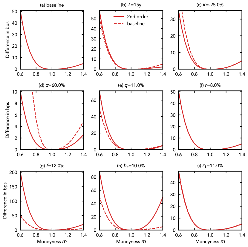
Figure 1: Error levels in basis points of notional for the forward approximation formula (84) as a function of the moneyness level $m$ defined in equation (82). Using the values in Table 1 as baseline in graph plot (a), we modify model parameters one by one across plots to assess how the approximation accuracy varies, varying other parameters as necessary to maintain no-arbitrage conditions from Proposition 2. The approximation is extremely accurate even for deviations of up to $\pm 40\%$ around the ATMRF level $m=1$; the error is even sharper for moneyness levels above 1 where the difference between the approximation and the exact formula does not go above 20bps. Higher volatility or WWR jump size materially decrease the error, whereas higher funding or stock repo rates can significantly increase it.

Our approximation formula allows for computation gains of same magnitude to those obtained for the ATM formula (80), compared to integrating numerically the exact formula (71). In terms of precision, we observe that the formula is very accurate across a wide range of moneyness levels $m$: Figure 1 in page 1 displays absolute errors between the exact formula (71) (calculated by integration) and the second-order approximation for different configurations of the model parameters, where the baseline scenario corresponds to the values displayed in Table 1 in page 1. Overall we observe errors are generally below 50bps even for moneyness values which are up to 40% away from the ATMRF level $K^{\star}$, hence the observed errors are significantly lower than order $\bar{m}^{3}$ which can be explained by the error contributions from each approximation within equation (84) counteracting each other. As noted above, errors noticeably decrease as the volatility $\sigma$ increases; moreover, we also observe a material upward bias in errors when $m<1$ compared to $m>1$ as expected, in fact for the latter case the error remains below 20bps of notional under all cases.

In view of the reported accuracy, the formula can effectively be used for obtaining quick estimates of the cost of entering trades which are near the ATM level – which comprises the majority of transactions. Such estimates enable sales and trading desks to quote accurate prices to clients and execute transactions at fair price levels, without having to resort to expensive Monte Carlo methods; in particular this formula could be integrated into electronic trading systems whereby requests for quotes (RFQ) from clients could be immediately fulfilled inclusive of credit and funding risks.

5 Numerical analysis for the valuation of the vulnerable forward contract

5.1 Setup for the numerical analysis

We now use Theorem 2 to perform comparative statics on the pre-default valuation of the vulnerable forward contract and identify model parameters exhibiting higher sensitivity, as well as any cross-effect between them. Without loss of generality we set $t=0$ – note that valuations only depend on the time to maturity $\mathcal{T}=T-t$.

We perform our analysis under two different settings. First, in order to remove the impact from the moneyness level of the forward, which arises from the terminal component in equation (71) and which normally dominates the valuation, we set the contract strike $K$ to the following value, which we call terminal at-the-money (TATM):

$$\hat{K}=se^{(\hat{r}_{S}-\kappa\hat{b}_{V})T}$$ (88)

Note that if equation (88) holds, the pre-default valuation from Theorem 2 becomes:

$$v(t,s) =-\hat{b}_{V}(1+\kappa)\int_{t}^{T}e^{-\hat{r}_{V}(u-t)}\hstretch{2}{\hat{\hstretch{.5}{\mathcal{BS}}}}_{P}\left(s,\frac{\mathcal{K}(u,\hat{K})}{1+\kappa},u-t\right)\mathrm{d}u$$

$$\qquad+(\hat{b}_{V}-b)(1+\kappa)\int_{t}^{T}e^{-\hat{r}_{V}(u-t)}\hstretch{2}{\hat{\hstretch{.5}{\mathcal{BS}}}}_{C}\left(s,\frac{\mathcal{K}(u,\hat{K})}{1+\kappa},u-t\right)\mathrm{d}u$$ (89)

Under this setting, if we modify any model parameter which changes the value $\hat{K}$, we also modify the value of the TATM strike accordingly so that the value of the terminal component remains zero; we call this setting constant terminal moneyness and it measures how the value arising from the call and put components evolves for a TATM contract (the most important case considering forward contracts tend to be struck ATM); it enables the dealer to assess how its quoted price would change if the assumed parameter values were to change. In our second setting, we set the baseline strike equal to $\hat{K}$ but we keep its value fixed even though we might modify parameters such as the repo rate or the WWR jump size: we call this setting constant terminal strike, and it illustrates how the vulnerable value evolves if market risk factors move.

For our analysis, we set the initial stock price $S_{0}=s$ to 1 throughout. This is equivalent to studying the following terminal payoff at expiry $T$:

$$\varphi\left(\frac{S_{T}}{S_{0}}\right)=\frac{S_{T}}{S_{0}}-K$$ (90)

The payoff (90) corresponds to an equity return forward. Such instruments, together with equity swaps have become increasingly popular among hedge funds and other investors in the last few years: analysis of financial statements (form FR Y-9C) reported by the five largest broker-dealers in the US to the Federal Reserve shows that the total notional of transactions classified as “equity swaps” held in their balance sheets increased from $1.3Tn in March 2016 to $2.7Tn in September 2021 – roughly a two-fold increase. By contrast, during the same period the figure for “interest rate swaps” decreased by more than 10%. In particular, equity swaps were the main trading instrument used by Archegos Capital Management, the fund which imploded spectacularly at the beginning of 2021, triggering large losses among its counterparties (Kinder & Lewis,, 2021; Lewis & Walker,, 2021). The increasing weight of such contracts among market participants, as well as the fact they are often traded by leveraged counterparties running speculative strategies, underlines the importance of measuring accurately both their default and wrong-way risks.

We now select baseline values for all our model parameters based on an analysis of empirical market data for observable risk factors which can be assimilated to our own model parameters such as S&P 500 implied volatility or USD LIBOR rates. We perform single-parameter sensitivity analysis by modifying these baseline inputs across a plausible range of values for that specific parameter and assessing how the contract value changes. We also produce three-dimensional plots where we analyse joint-sensitivities to a simultaneous change in two distinct model parameters, allowing us to identify any salient cross-effect between parameters.

Table 1 shows the baseline values for the model, as well as the sensitivity range for single-parameter analysis – for joint-sensitivities, we sometimes widen the range of values to reveal the relationship between two different inputs. Note our goal is to investigate which risk factors are more critical from a risk management perspective by analysing the magnitude and direction of price sensitivities; hence no-arbitrage conditions from Proposition 2 might not hold over all value combinations implied by the ranges in Table 1. We note that conditions (74), (75) and (76) from Corollary 2 hold for all baseline values of model parameters as well as across all the sensitivity ranges.

Variable	Base value	Sensitivity range
Stock price $s$	1.0	–
Expiry $T$	5y	[1, 30]
Dividend rate $q$	5.5%	[0%, 15%]
Volatility $\sigma$	30.0%	[5%, 80%]
Risk-free rate $r$	4.0%	[$-$3%, 15%]
Funding rate $f$	6.0%	[0%, 15%]
Repo rate $h_{S}$	5.0%	[0%, 15%]
Repo rates $h_{i}$	5.5%	[0%, 15%]
Bond rates $r_{i}$	7.0%	[0%, 15%]
WWR jump rate $\kappa$	0%	[$-$50%, 0%]
Funding policy $\alpha$	0.5	[0, 1]
Recovery rates $\varkappa_{i}$	100%	–

Table 1: Baseline values for numerical analysis.

In order to compare derivative prices across different parameters values, we need to define an appropriate normalised metric. We have explained that the forward contract can be interpreted as a forward on the stock return, for which it is industry practice to express costs in terms of yearly basis points (bps) of notional. The advantage of this metric is that it is insensitive to the size of the trade; the initial stock value $s$; and also to the length $T$ of the deal, which is important in our framework because longer contracts will naturally exhibit larger default and funding risk: for example, the longer the contractual relationship with a certain counterparty, the higher the likelihood she will default during that time frame. Formally, we look at the quantity:

$$\frac{v(t,s)}{s(T-t)}=\frac{v(0,1)}{T}$$ (91)

where we have used our standing numerical assumptions in this section that $t=0$ and $s=1$.

5.2 Single-parameter sensitivity analysis

5.2.1 Constant terminal moneyness

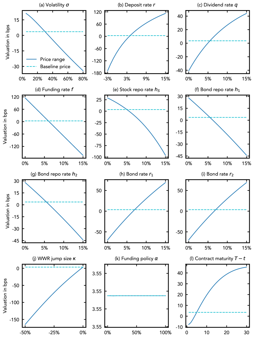
Figure 2: Single-parameter sensitivity analysis across model parameters based on the value ranges displayed in Table 1, with constant terminal moneyness (CTM), plotted against the baseline case calculated with the values from the table. We do not enforce the no-arbitrage restrictions and strictly keep all other parameters fixed, as our purpose is to assess price sensitivity. The y-axis displays the value of metric (91). We observe sensitivity is highest against the deposit $r$ and funding $f$ rates; the concave sensitivity to maturity $T-t$ as observed in graph (l) is explained by the discounting terms within integrals (89), which decrease exponentially any incremental area contributed by the integrand as the integration bound $T$ increases.

Figure 2 in page 2 displays comparative statics across our model parameters when we set the contract strike to $\hat{K}$ from equation (88) and keep moneyness constant across changes in parameters. Values are benchmarked against the contract’s baseline value which is 3.55 bps/year hence 17.74 bps across the deal’s life – by contrast, in a risk-free setting with no default, funding or WWR risk factors, the cost to enter an at-the-money forward contract would be null.

We make the following highlights:

1. Valuation sensitivity is higher for lending/borrowing parameters than credit parameters: we observe that the change in price with respect to the deposit (or risk-free) rate $r$ and the funding rate $f$ is larger than for other inputs, with valuations varying approximately across a 250-300 bps/year range, which represents 2.5% to 3.0% of the trade notional on an annual basis. On the other hand, varying the bond rates from 0% to 15% modifies the valuation by around 120 bps/year. While the order of magnitude is similar, we can state sensitivity to funding is roughly double that to credit parameters.

2. Vulnerable forwards exhibit sensitivity to stock volatility: the cost to enter the vulnerable forward varies within a 60 bps/year range when we change the stock volatility $\sigma$ from close to 0% to 80%. It is worth insisting that, contrary to the case of risk-free valuation where linear products such as forwards do not exhibit sensitivity to volatility, in a framework equipped with counterparty risks the pricing of even simple products becomes dependant on this model parameter. The implication is that vulnerable forwards are contingent assets, that is certain cash flows only arise under specific circumstances. Here, the non-linear term $b\max\{z_{\kappa},0\}$ from the linearised PDE (48) represents such a contingent cash-flow which only occurs when $z(t,s(1+\kappa))<0$. One important fact about contingent contracts is there does not exist a static trading strategy in linear assets which hedges them (Shin,, 2019). We could show that under asymmetric recovery rates, that is $\varkappa_{1}\neq\varkappa_{2}$, there is additional cash-flow contingency.

3. Wrong-way risk can be a material risk in specific deals: the WWR jump size is a material risk factor with valuation varying within a 150 bps/year range when we change $\kappa$ from 0 to $-$50% (roughly the same order of sensitivity than bond repo or credit rates) such that each additional percentage point of jump size moving the forward price by around 3.4bps/year. Recall that by Proposition 1, parameter $\kappa$ can be interpreted as controlling stock-default correlation; hence in the presence of dependency between the contracting parties and the underlying asset referenced by $\hstretch{2}{\hat{\hstretch{.5}{\mathcal{D}}}}_{1}$, failure to account for such correlation can materially misrepresent the risk profile of the transaction. More generally, this parameter can be fine-tuned in specific transactions where the broker-dealer is aware of adverse correlation between stock price movements and counterparty credit quality which might materially impact the change in value from the contract at the time of default.

5.2.2 Constant terminal strike

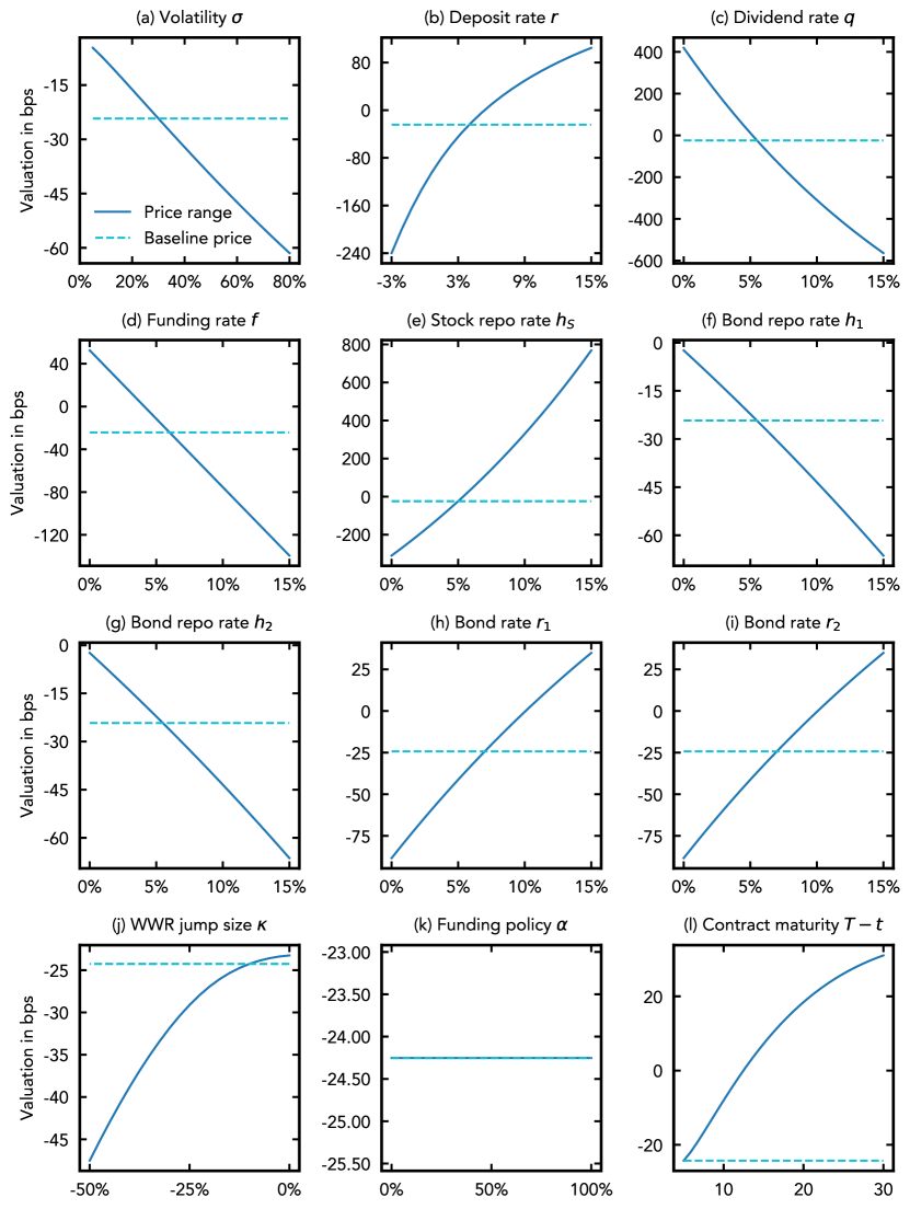
Figure 3: Single-parameter sensitivity analysis across model parameters based on the value ranges displayed in Table 1, with constant terminal strike (CTS), plotted against the baseline case calculated with the values from the table (except for $\kappa$ which has been set to $-10\%$). We do not enforce the no-arbitrage restrictions and strictly keep all other parameters fixed, as our purpose is to assess price sensitivity. The y-axis displays the value of metric (91). Sensitivity is very pronounced for dividend $q$ and stock repo $h_{S}$ rates which are the main parameters driving the risky stock forward (92).

Figure 3 in page 3 displays a similar analysis as in the previous section, but by keeping the terminal ATM strike $\hat{K}$ constant even though the underlying model parameters are modified. To reveal the full spectrum of sensitivities (in particular the interaction between WWR and bond parameters), we have modified the baseline value of the WWR parameter $\kappa$ to $-$10%. In this scenario, the baseline value for the contracts changes to $-$24.25 bps/year and $-$121.27 bps in total.

To interpret our results, we define the risky stock forward $\hat{s}:\mathbb{R}_{+}^{2}\rightarrow\mathbb{R}_{+}$ as follows:

$$\hat{s}(s,\mathcal{T}):=se^{(\hat{r}_{S}-\kappa\hat{b}_{V})\mathcal{T}}$$ (92)

where under our settings $s=1$ and $\mathcal{T}=T$. In the constant strike case, only parameters which modify the value arising from the terminal component – in particular the risky forward – will have a different sensitivity than under the constant moneyness setup. In particular recalling that $\alpha_{S}^{\ast}=-\kappa$:

$$\hat{r}_{S}-\kappa\hat{b}_{V} =(1+\kappa)h_{S}-q+\kappa((\alpha h_{1}+(1-\alpha)h_{2})-(r_{1}+r_{2}))$$ (93)

We make the following observations, which highlight the differences with the constant moneyness case:

1. Stock repo and bond return rates push up the risky forward: because $\kappa\in(-1,0]$ heightening the stock repo rate or the bond rates effectively increases the vulnerable stock forward $\hat{s}(1,T)$ above the contract strike, thereby increasing the value of the terminal cash flow in case of no default.

2. Dividend rate and bond repo rates have the opposite effect: on the other hand, an increase in the dividend rate or the bond repo rates lower the risky forward below the strike and decrease the terminal value.

3. Changes in WWR shift sensitivity to credit risk factors: from the decomposition (93) and the plots in Figure 3, we also observe that increasing the WWR jump size $\kappa$ lowers the weight of the stock repo while increasing that from the bond repo and return rates: more generally, higher wrong-way risk increases the sensitivity to credit parameters as we will show in the next section.

The behaviour from the stock repo and dividend rates is consistent with that observed under no credit or funding risks: by modifying the funding rate for the hedging strategy (that is the stock repo rate) or the benefits received (dividends) we change the moneyness of the forward contract – namely its intrinsic value. We also observe this intrinsic value dominates any value arising from the contingent cash flow induced by recovery payouts or asymmetric funding rates: when keeping the strike constant, the valuation sensitivity to $h_{S}$ and $q$ is much higher than for the rest, with values varying over a range of almost 10%/year for both parameters.

One important implication from the above is for contracts referencing distressed names: a worsening outlook on the economic prospects of a company will tend to increase short positions on its stock, exerting upward pressure on its repo rate (usually known as “specials” in industry parlance) and materially affecting the contract valuation.

5.3 Joint-sensitivity analysis

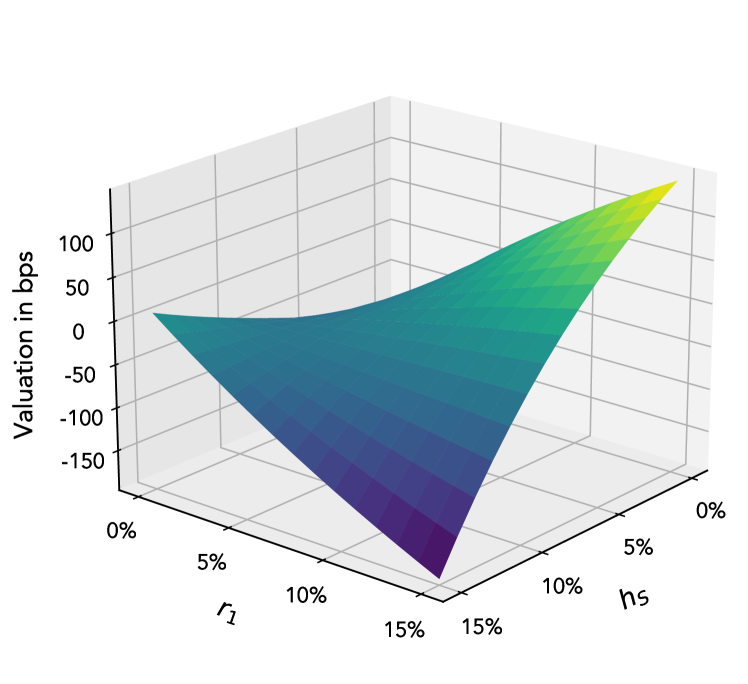
(a) Bond rate $r_{1}$ vs. stock repo $h_{S}$

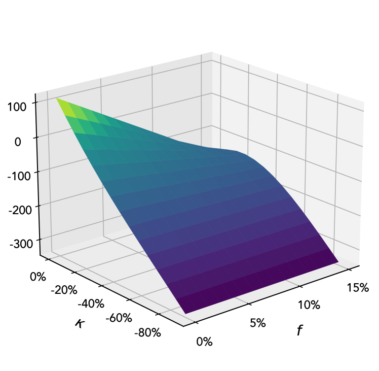
(b) WWR jump $\kappa$ vs. funding rate $f$

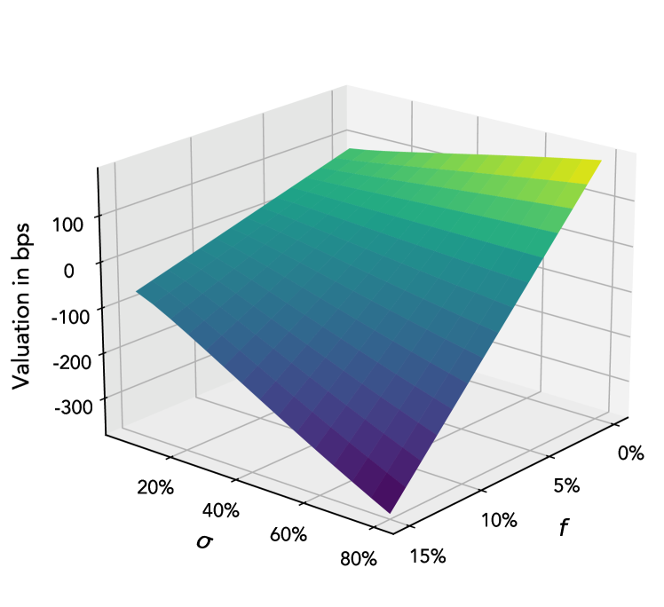
(c) Volatility $\sigma$ vs. funding rate $f$

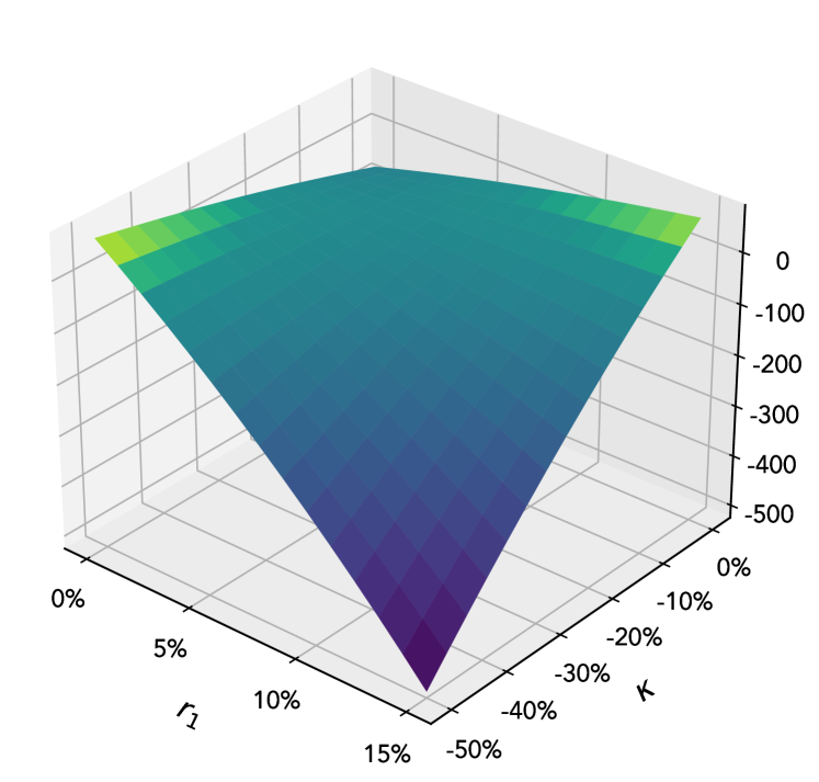
(d) Bond rate $r_{1}$ vs. WWR jump $\kappa$

Figure 4: Joint-sensitivity analysis across selected pairs of model parameters. The y-axis displays the value of metric (91); colouring is based on distance to the baseline value.

Figure 4 in page 4 displays comparative statics across selected pairs of model parameters, where in some cases we have extended the value ranges from Table 1 to illuminate more prominently any relevant cross-effects. We work under the constant terminal moneyness assumption so that the TATM strike changes with parameters in order for $m$ to stay equal to 1.

We make the following highlights:

1. Sign of sensitivity to bond rates $r_{i}$ and the stock repo rate $h_{S}$ are dependent on each other: Surface 4(a) plots the valuation (in bps of notional) against different values for the bond rate $r_{1}$ and the repo rate $h_{S}$. We observe that the direction of sensitivity to each parameter changes depending on the value of the other parameter: for example sensitivity to the repo rate $h_{S}$ is more pronounced when the bond rate $r_{1}$ stands at 15%, with valuation decreasing from around 125bps down to $-$150bps as we vary the repo rate from close to 0% up to 15%; however when the credit rate goes to zero, the sensitivity range for $h_{S}$ tightens and we observe the direction changes, with the valuation becoming increasing in the repo rate. The same phenomenon is observed for the credit rate $r_{1}$. In periods of market stress where credit spreads widen and repo rates can spike, the risk profile of vulnerable forwards can suddenly flip; the sharp sensitivity to the repo rate $h_{S}$ under high credit spreads suggests the derivative dealer should pay particular attention to its repo risk for stocks or currencies for which the borrowing cost is high.

2. Sensitivity to the funding rate vanishes under extreme WWR risk: as show in Figure 4(b) the sensitivity of the forward valuation to the dealer’s funding rate $f$ vanishes very quickly as the WWR jump size $\kappa$ decreases down to $-$90%. In specific transactions where WWR is particularly acute, managing this risk becomes much more critical than any funding cost arising from the dealer’s funding spread. These results highlight again the importance of modelling wrong-way/gap risks as well as stock-credit correlations for derivative transactions where there is default risk from either counterparty.

3. Simultaneous increases of the funding rate $f$ and volatility $\sigma$ feed each other: Graph 4(c) demonstrates the valuation can be subject to violent changes in situations of market stress, where funding spreads might widen and volatilities spike up. Sensitivity to volatility goes to zero as the funding rate converges to the deposit rate $r$ (whose baseline value is 4%) which is expected: the sensitivity to $f$ arises from cash flow contingency, yet without volatility there is no randomness and future cash flows are known since inception. When volatility and the funding spread reach very high levels, the difference with our baseline value is close to 300 bps. A potential scenario reflective of this observation is a liquidity crisis in the banking sector, where market funding costs spike and stock volatility shots up.

4. Widening credit spreads combined with high wrong-way risk lead to a strong fall in TATM prices: Figure 4(d) illustrates a catastrophic scenario where widening credit spreads coupled with a sharp increase in wrong-way risk can drive a large fall in the contract’s TATM valuation from between 0 to $-$50bps all the way down to around $-$500bps. This scenario is another illustration of how important it is to account for any potential wrong-way risk: for counterparties exhibiting higher default risk than usual, the dealer needs to be particularly careful about its WWR assumptions to avoid materially misrepresenting the credit risk embedded in the transaction.

6 Conclusions

In this paper we have presented a market model which incorporates ab initio funding, credit and wrong-way risk factors using a mixed Brownian-Poisson model for price dynamics and defaults.

We have derived a trading strategy which allows a dealer contracting a vulnerable derivative to hedge away any such risks. From this strategy and the theory of derivative valuation, we find a non-linear PDE whose solution determines the pre-default valuation of the vulnerable contract and we determine conditions on the funding policy under which the PDE become linear, see Proposition 4 and Corollary 1. An application of the Feynman-Kac theorem allows us to characterize the solution to the pre-default valuation problem as a conditional expectation under a pricing measure $\widehat{\mathbb{Q}}$ in Theorem 1.

We deploy the previous framework to the specific problem of valuing a vulnerable forward contract on a stock. We find that the pre-default valuation can be expressed as a portfolio over a continuum of European call and put options valued under measure $\widehat{\mathbb{Q}}$ thereby obtaining an analytical formula involving double Gaussian integrals, as established in Theorem 2. The previous valuation formula is simplified when the forward is at-the-money with respect to the market risk-free rate $r$, so that the pre-default value can be expressed as a linear combination of Gaussian integrals – see Corollary 2. Although no formula exists for the general case where the strike can be any value, in Theorem 3 we derive a second order approximation in moneyness which is shown empirically to be very precise, with errors below 0.5% of notional even for deviations of up to $\pm$40% from the ATM case.

Finally, we have performed sensitivity analysis to different model parameters and made three important conclusions: first, deposit/funding rates are the most material risk factors for contracts whose terminal component is at-the-money; secondly, valuations exhibit high sensitivity to wrong-way risk and neglecting it can materially undervalue the contract; thirdly, wrong-way risk and credit spreads exhibit strong joint sensitivity and can generate sharp moves in valuation when both evolve adversely.

Our research demonstrates it is possible to compute in closed-form the price of derivative contract with bilateral cash flows, including ab initio any credit or funding risk factor, without needing to resort to individual credit or funding valuation adjustments. These findings can be used for industrial applications such as swift quoting of all-inclusive derivative prices to clients, instead of relying on valuation engines based on slow Monte Carlo simulations. Moreover, our representation of the contract price in terms of a portfolio of options illustrates the inherent optionality in contracts where there is default risk and asymmetric rates, and suggests alternative strategies for hedging such risks.

Appendix A Figures

Appendix B Mathematical proofs

B.1 Proof of Proposition 1

Proof.

Throughout the proof we work under the probability measure $\mathbb{P}$. The solution to the SDE (6) for the stock price $S$ is well-known (Merton,, 1976):

$$S_{t}=s\exp\left\{\left(\mu-q-\frac{\sigma^{2}}{2}\right)t+\sigma W_{t}\right\}\left(1+\kappa J_{t}\right)$$ (94)

with $S_{0}=s$. Let us define the continuous part process $S^{0}$ of the stock price as:

$$S^{0}_{t}=s\exp\left\{\left(\mu-q-\frac{\sigma^{2}}{2}\right)t+\sigma W_{t}\right\}$$ (95)

Note that $S^{0}$ and $J$ are independent because we have assumed the Brownian motion $W$ and the Poisson processes to be independent. Therefore by bilinearity, the covariance between the stock price and the default event is equal to:

$$\mathbb{C}\mathrm{ov}\left(S_{t},J_{t}\right) =\mathbb{C}\mathrm{ov}(S^{0}_{t}(1+\kappa J_{t}),J_{t})$$

$$=\kappa\mathbb{E}(S^{0}_{t})\mathbb{V}\mathrm{ar}(J_{t})$$ (96)

Equation (7) directly ensues. Additionally, we can compute expression (96) in closed-form. We recall that the sum of two independent Poisson process is a Poisson process with intensity equal to the sum of the intensities from its components; therefore the first-to-default process $J$ is induced by a Poisson process $N$ defined as $N:=N^{(1)}+N^{(2)}$ with intensity $\lambda:=\lambda_{1}+\lambda_{2}$. Hence the expectation and variance of $J$ are given by:

$$\mathbb{E}\left(J_{t}\right) =\mathbb{P}\left(\tau\leq t\right)=1-e^{-\lambda t}$$ (97)

$$\mathbb{V}\mathrm{ar}\left(J_{t}\right) =\mathbb{E}\left(J_{t}\right)-\mathbb{E}\left(J_{t}\right)^{2}=e^{-\lambda t}(1-e^{-\lambda t})$$ (98)

Let us define for $t\in[0,\bar{T}]$:

$$p_{J}(t):=1-e^{-\lambda t}$$ (99)

which corresponds to the probability of the first default happening at or before $t$. By independence of $S^{0}$ and $J$, the second moment of the stock price is equal to:

$$\mathbb{E}(S_{t}^{2}) =s^{2}e^{(2(\mu-q)+\sigma^{2})t}(1+\kappa p_{J}(t)(2+\kappa))$$ (100)

On the other hand:

$$\mathbb{E}(S_{t})^{2} =s^{2}e^{2(\mu-q)t}(1+\kappa p_{J}(t)(2+\kappa p_{J}(t)))$$

Therefore the variance of $S$ is equal to:

$$\mathbb{V}\mathrm{ar}(S_{t})=s^{2}e^{2(\mu-q)t}\big{(}e^{\sigma^{2}t}(1+\kappa p_{J}(t)(2+\kappa))-(1+\kappa p_{J}(t)(2+\kappa p_{J}(t)))\big{)}$$ (101)

Using equations (98) and (96), we derive the closed-form expression for stock-default correlation:

$$\rho_{S,J}(t) =\kappa\sqrt{\frac{p_{J}(t)(1-p_{J}(t))}{e^{\sigma^{2}t}(1+\kappa p_{J}(t)(2+\kappa))-(1+\kappa p_{J}(t)(2+\kappa p_{J}(t)))}}$$ (102)

Note that for $\kappa$ near 0 we can make the following approximation for the denominator in (102):

$$e^{\sigma^{2}t}(1+\kappa p_{J}(t)(2+\kappa))-(1+\kappa p_{J}(t)(2+\kappa p_{J}(t)))=(1+2\kappa p_{J}(t))(e^{\sigma^{2}t}-1)+\mathcal{O}(\kappa^{2})$$ (103)

Therefore for $\kappa$ near 0:

$$\rho_{S,J}(t)\approx a(t)\kappa\sqrt{\frac{1}{1+2\kappa p_{J}(t)}}$$ (104)

where the function $a:t\mapsto a(t)$ depends on $\lambda$ and $\sigma$. Moreover using the following Taylor expansion for $x\in\mathbb{R}$ near 0:

$$\frac{1}{1+x}=1-x+\mathcal{O}(x^{2}),$$ (105)

we refine further the approximation (104):

$$a(t)\kappa\sqrt{\frac{1}{1+2\kappa p_{J}(t)}}\approx a(t)\kappa\sqrt{1-2\kappa p_{J}(t)}$$ (106)

A final approximation of (106) in $\kappa$ by neglecting terms of order $\mathcal{O}(\kappa^{2})$ allows us to conclude. ∎

B.2 Proof of Proposition 2

Proof.

Proposition 2 states a necessary condition for $\mathfrak{M}$ to be arbitrage-free hence it suffices to prove that if conditions (18)-(19) are not fulfilled, then there exists arbitrage opportunities. To prove (18) is a necessary condition, without loss of generality let us consider $h=h_{S}$ and a trading strategy $\Theta$ such that $\upvartheta^{S}_{t}\geq 0$ for all $t$ and:

$$\theta^{S}_{t}=-\upvartheta^{S}_{t},\qquad\theta^{B}_{t}=\frac{\upvartheta^{S}_{t}S_{t}}{B_{t}}$$ (107)

while the rest of the elements of $\Theta$ are null, then:

$$\Pi^{\Theta}_{0}=0,\qquad\mathrm{d}G^{\Theta}_{t}=(r-h_{S})\upvartheta^{S}_{t}S_{t}\mathrm{d}t$$ (108)

which is an arbitrage if $r>h_{S}$. To show that $f<h_{S}$ entails arbitrage opportunities, it suffices to consider instead the portfolio with $\vartheta^{S}_{t}\leq 0$ and:

$$\theta^{S}_{t}=-\upvartheta^{S}_{t},\qquad\theta^{F}_{t}=\frac{\upvartheta^{S}_{t}S_{t}}{F_{t}}$$ (109)

The same reasoning is applicable to the bond repo rates $h_{1}$ and $h_{2}$ thus establishing the necessity of (18). To prove (19) is necessary, consider an alternative strategy $\Theta$ with $\vartheta^{(i)}_{t}\leq 0$ and the rest of units being null such that:

$$\Pi^{\Theta}_{0}=0,\qquad\mathrm{d}G^{\Theta}_{t}=P^{(i)}_{t^{-}}((h_{i}-r_{i})\mathrm{d}t+\mathrm{d}J^{(i)}_{t})$$ (110)

If $h_{i}\geq r_{i}$ then the strategy receives a continuous positive cash flow stream $P^{(i)}_{t^{-}}(h_{i}-r_{i})\mathrm{d}t$ until default $\tau$ where it pays out the positive lump sum $P^{(i)}_{\tau}$ which constitutes an arbitrage. ∎

B.3 Proof of Lemma 1

Proof.

The continuous component $\tilde{S}$ of the stock price (94) (see page 94) can be expressed a twice-continuously differentiable function of time $t$ and the Brownian Motion $W$ which is a semimartingale by Corollary 3 in Section 3 of Chapter II from Protter, (1990) hence this continuous component is also a semimartingale process per Itô’s Formula (Theorem 32, Chapter II in Protter,, 1990); additionally, the jump component of (94) is a finite variation process hence it is also a semimartingale (Section 8.1.1 in Cont & Tankov,, 2004). As $S$ is the product of two semimartingales, it is also a semimartingale (Corollary 2, Section 6 of Chapter II in Protter,, 1990). Moreover, by assumption the processes $V$ and $Z$ are defined as twice-continuously differentiable functions evaluated at $(t,S_{t})$ thus they are also semimartingales by Itô’s Lemma. We can use the integration by parts formula for semimartingales (Corollary 2, Chapter II in Protter,, 1990) and $1-J_{0}=1$:

$$(1-J_{t})V_{t}=V_{0}-\int_{0}^{t}V_{u^{-}}\mathrm{d}J_{u}+\int_{0}^{t}(1-J_{u^{-}})\mathrm{d}V_{u}-[J,V]_{t}$$ (111)

We have shown $V$ is a semimartingale; moreover, $J$ is a process of finite variation hence we have (see Lemma 3, Section “Properties of Quadratic Variations” in Lowther,, 2009):

$$[J,V]_{t}=\int_{0}^{t}\Delta V_{u}\mathrm{d}J_{u}$$ (112)

By the same arguments and $J_{0}=0$:

$$J_{t}Z_{t}=\int_{0}^{t}Z_{u^{-}}\mathrm{d}J_{u}+\int_{0}^{t}J_{u^{-}}\mathrm{d}Z_{u}+\int_{0}^{t}\Delta Z_{u}\mathrm{d}J_{u}$$ (113)

where we define $\Delta Z_{t}:=Z_{t}-Z_{t^{-}}$. Summing (111) and (113) and using the definition of $\Delta Z$ we obtain an expression for $\hat{V}_{t}$:

$$\hat{V}_{t} =\hat{V}_{0}+\int_{0}^{t}(1-J_{u^{-}})\mathrm{d}V_{u}-\int_{0}^{t}\Delta V_{u}\mathrm{d}J_{u}+\int_{0}^{t}(Z_{u}-V_{u^{-}})\mathrm{d}J_{u}+\int_{0}^{t}J_{u^{-}}\mathrm{d}Z_{u}$$ (114)

The stopped valuation process is therefore equal to:

$$\hat{V}^{\tau}_{t} =\hat{V}_{0}+\int_{0}^{t\wedge\tau}(1-J_{u^{-}})\mathrm{d}V_{u}-\int_{0}^{t\wedge\tau}\Delta V_{u}\mathrm{d}J_{u}+\int_{0}^{t\wedge\tau}(Z_{u}-V_{u^{-}})\mathrm{d}J_{u}+\int_{0}^{t\wedge\tau}J_{u^{-}}\mathrm{d}Z_{u}$$ (115)

Note that $J_{u^{-}}=0$ for $u\leq\tau$ hence the last integral is equal to 0. Combining the second and third integrals and using the definition of process $\widehat{L}=Z-V_{-}$ we get the following expression for $\hat{V}^{\tau}$:

$$\hat{V}^{\tau}_{t} =\hat{V}_{0}+\int_{0}^{t}\mathbbm{1}_{\{u\leq\tau\}}(1-J_{u^{-}})\mathrm{d}V_{u}+\int_{0}^{t}\mathbbm{1}_{\{u\leq\tau\}}(\widehat{L}_{u}-\Delta V_{u})\mathrm{d}J_{u}$$ (116)

By observing that $\mathbbm{1}_{\{u\leq\tau\}}=(1-J_{u^{-}})$ we conclude. ∎

B.4 Proof of Lemma 2

Proof.

Equations (36) and (37) for processes $\theta^{B}$ and $\theta^{F}$ respectively are a direct consequence of Proposition 3 and the hedging condition (29a). The strategy in the stock (34) is derived by matching the term in $\mathrm{d}S_{t}$ from the claim dynamics (31) with that from the portfolio gain process (33):

$$\mathrm{d}\hat{V}^{\tau}_{t}=\mathbbm{1}_{\{t\leq\tau\}}v_{s}(t,S_{t^{-}})\mathrm{d}S_{t}+\dots,\quad\quad\quad\mathrm{d}G^{\Theta}_{t}=(\theta^{S}_{t}+\upvartheta^{S}_{t})\mathrm{d}S_{t}+\dots$$ (117)

To derive the strategy (35) for the bonds, we start by rewriting the jump component of the stopped valuation process from equation (31) using the definitions of $\widehat{L}$ and $J$:

$$\mathbbm{1}_{\{t\leq\tau\}}\left(\widehat{L}_{t}-v_{s}(t,S_{t^{-}})\Delta S_{t}\right)\mathrm{d}J_{t}=$$

$$\qquad\mathbbm{1}_{\{t\leq\tau\}}\left(Z_{t}-V_{t^{-}}-v_{s}(t,S_{t^{-}})\Delta S_{t}\right)\mathrm{d}(J^{(1)}_{t}+J^{(2)}_{t}-J^{(1)}_{t}J^{(2)}_{t})$$ (118)

Observe that $\mathbbm{1}_{\{t\leq\tau\}}\mathrm{d}(J^{(1)}_{t}J^{(2)}_{t})=0$ given the default processes cannot jump simultaneously; moreover we have assumed $\kappa_{1}=\kappa_{2}=\kappa$ thus at the time of any jump we have $Z_{t}=Z_{t^{-}}+\Delta Z_{t}=z(t,(1+\kappa)S_{t^{-}})$; finally, $\Delta S_{t}=S_{t}-S_{t^{-}}=\kappa S_{t^{-}}$. It comes:

$$\mathbbm{1}_{\{t\leq\tau\}}\left(\widehat{L}_{t}-v_{s}(t,S_{t^{-}})\Delta S_{t}\right)\mathrm{d}J_{t}=$$

$$\qquad\mathbbm{1}_{\{t\leq\tau\}}\left(z(t,(1+\kappa)S_{t^{-}})-v(t,S_{t^{-}})-v_{s}(t,S_{t^{-}})\kappa S_{t^{-}}\right)(\mathrm{d}J^{(1)}_{t}+\mathrm{d}J^{(2)}_{t})$$ (119)

It then suffices to split the price changes $\mathrm{d}P^{(i)}_{t}$ into their drift and jump components, and match the jump components with the term (119):

$$(\theta^{(i)}_{t}+\upvartheta^{(i)}_{t})\mathrm{d}P^{(i)}_{t}=-(\theta^{(i)}_{t}+\upvartheta^{(i)}_{t})P^{(i)}_{t^{-}}\mathrm{d}J^{(i)}_{t}+\dots$$ (120)

∎

B.5 Proof of Proposition 4

Proof.

To compact notation for the purposes of this proof, we introduce the continuous function $\widehat{l}:[0,T]\times\mathbb{R}_{+}^{*}\rightarrow\mathbb{R}$ defined for $(t,s)$:

$$\widehat{l}(t,s):=z(t,(1+\kappa)s)-v(t,s)$$ (121)

In particular note that $\widehat{L}_{\tau}=\widehat{l}(\tau,S_{\tau^{-}})$.

In expression (33) for the gain process $G^{\Theta}$ of the portfolio, we expand the differentials for the stock dividends $\mathrm{d}D_{t}$, the bond prices $\mathrm{d}P^{(i)}_{t}$ and the bank accounts $\mathrm{d}D_{t}$ and $\mathrm{d}F_{t}$ – where we recall the expressions are given in Section 2.1, equations (9), (5) and (3)-(4) respectively:

$$\mathrm{d}G^{\Theta}_{t} =(\theta^{S}_{t}+\upvartheta^{S}_{t})\mathrm{d}(S_{t}+qS_{t^{-}}\mathrm{d}t)-(\theta^{(1)}_{t}+\upvartheta^{(1)}_{t})P^{(1)}_{t^{-}}\mathrm{d}J^{(1)}_{t}-(\theta^{(2)}_{t}+\upvartheta^{(2)}_{t})P^{(2)}_{t^{-}}\mathrm{d}J^{(2)}_{t}$$

$$\quad+r_{1}(\theta^{(1)}_{t}+\upvartheta^{(1)}_{t})P^{(1)}_{t^{-}}\mathrm{d}t+r_{2}(\theta^{(2)}_{t}+\upvartheta^{(2)}_{t})P^{(2)}_{t^{-}}\mathrm{d}t-\left(h_{S}\upvartheta^{S}_{t^{-}}S_{t}+h_{1}\upvartheta^{(1)}_{t}P^{(1)}_{t^{-}}+h_{2}\upvartheta^{(2)}_{t}P^{(2)}_{t^{-}}\right)\mathrm{d}t$$

$$\quad+r\theta^{B}_{t}B_{t}\mathrm{d}t+f\theta^{F}_{t}F_{t}\mathrm{d}t$$ (122)

We now replace the units invested in the market assets (stock, bonds, repos, bank accounts) by the expressions given in Lemma 2. First note that using the definition of the funding policy $\alpha_{S}$ from (38) we have the following equality for the stock repo strategy:

$$\upvartheta^{S}_{t}S_{t}=(1-\alpha_{S})(\theta^{S}_{t}+\upvartheta^{S}_{t})S_{t}=-\mathbbm{1}_{\{t\leq\tau\}}(1-\alpha_{S})v_{s}(t,S_{t^{-}})S_{t}$$ (123)

Similarly for the defaultable bonds, with $i\in\{1,2\}$:

$$\upvartheta^{(i)}_{t}P^{(i)}_{t}=\mathbbm{1}_{\{t\leq\tau\}}(1-\alpha_{i})(\widehat{l}(t,S_{t^{-}})-v_{s}(t,S_{t^{-}})\kappa S_{t^{-}})$$ (124)

We rearrange (122) by combining terms in $\mathrm{d}t$:

$$\mathrm{d}G^{\Theta}_{t} =-\mathbbm{1}_{\{t\leq\tau\}}v_{s}(t,S_{t^{-}})\mathrm{d}S_{t}-\mathbbm{1}_{\{t\leq\tau\}}(\widehat{l}(t,S_{t^{-}})-v_{s}(t,S_{t^{-}})\kappa S_{t^{-}})\mathrm{d}(J^{(1)}_{t}+J^{(2)}_{t})$$

$$\quad+\mathbbm{1}_{\{t\leq\tau\}}(r_{1}-(1-\alpha_{1})h_{1}+r_{2}-(1-\alpha_{2})h_{2})(\widehat{l}(t,S_{t^{-}})-v_{s}(t,S_{t^{-}})\kappa S_{t^{-}})\mathrm{d}t$$

$$\quad+\mathbbm{1}_{\{t\leq\tau\}}((1-\alpha_{S})h_{S}-q)S_{t^{-}}v_{s}(t,S_{t^{-}})\mathrm{d}t+r\max\{C^{\Theta}_{t},0\}\mathrm{d}t+f\min\{C^{\Theta}_{t},0\}\mathrm{d}t$$ (125)

where we have introduced the cash balance process $C^{\Theta}:\Omega\times[0,T]\rightarrow\mathbb{R}$ of the strategy, defined as:

$$C^{\Theta}_{t}:=-\mathbbm{1}_{\{t\leq\tau\}}\hat{V}^{\tau}_{t^{-}}-\theta^{S}_{t}S_{t^{-}}-\theta^{(1)}_{t}P^{(1)}_{t^{-}}-\theta^{(2)}_{t}P^{(2)}_{t^{-}}$$ (126)

Note that from Lemma 2 and the definition of the funding policies:

$$\theta^{(1)}_{t}P^{(1)}_{t^{-}}+\theta^{(2)}_{t}P^{(2)}_{t^{-}}=\mathbbm{1}_{\{t\leq\tau\}}(\alpha_{1}+\alpha_{2})(\widehat{l}(t,S_{t^{-}})-v_{s}(t,S_{t^{-}})\kappa S_{t^{-}})$$ (127)

On the other hand we have $\theta^{S}_{t}=-\mathbbm{1}_{\{t\leq\tau\}}\alpha_{S}v_{s}(t,S_{t^{-}})$; defining $\alpha_{1,2}:=\alpha_{1}+\alpha_{2}$ we get:

$$-\theta^{S}_{t}S_{t^{-}}-\theta^{(1)}_{t}P^{(1)}_{t^{-}}-\theta^{(2)}_{t}P^{(2)}_{t^{-}} =\mathbbm{1}_{\{t\leq\tau\}}\left(\alpha_{S}v_{s}(t,S_{t^{-}})S_{t^{-}}-\alpha_{1,2}(\widehat{l}(t,S_{t^{-}})-v_{s}(t,S_{t^{-}})\kappa S_{t^{-}})\right)$$ (128)

Moreover, using the definition of the stopped process (27), note that:

$$\mathbbm{1}_{\{t\leq\tau\}}\hat{V}^{\tau}_{t^{-}}=\mathbbm{1}_{\{t\leq\tau\}}\left(\mathbbm{1}_{\{t\leq\tau\}}V_{t^{-}}+\mathbbm{1}_{\{t>\tau\}}Z_{\tau}\right)=\mathbbm{1}_{\{t\leq\tau\}}V_{t^{-}}$$ (129)

So that by combining (128) and (129) we write $C^{\Theta}$ as:

$$C^{\Theta}_{t}=\mathbbm{1}_{\{t\leq\tau\}}\left(-V_{t^{-}}+\alpha_{S}v_{s}(t,S_{t^{-}})S_{t^{-}}-\alpha_{1,2}(\widehat{l}(t,S_{t^{-}})-v_{s}(t,S_{t^{-}})\kappa S_{t^{-}})\right)$$ (130)

We introduce the funding spread $b=f-r$ which is positive by Proposition 2. Then we can rearrange the positive and negative cash balance components in (125) as follows:

$$r\max\{C^{\Theta}_{t},0\}\mathrm{d}t+f\min\{C^{\Theta}_{t},0\}\mathrm{d}t=rC^{\Theta}_{t}\mathrm{d}t+b\min\{C^{\Theta}_{t},0\}\mathrm{d}t$$ (131)

Because $\mathbbm{1}_{\{t\leq\tau\}}\geq 0$ we can remove the indicator from within the minimum operator and factorize this term across the expression for the gain process $G^{\Theta}$; injecting equations (130) and (131) into (125), we obtain:

$$\mathrm{d}G^{\Theta}_{t} =\Big{(}-v_{s}(t,S_{t^{-}})\mathrm{d}S_{t}-(\widehat{l}(t,S_{t^{-}})-v_{s}(t,S_{t^{-}})\kappa S_{t^{-}})\mathrm{d}(J^{(1)}_{t}+J^{(2)}_{t})$$

$$\quad-rV_{t^{-}}\mathrm{d}t-(\hat{b}_{1}+\hat{b}_{2})(\widehat{l}(t,S_{t^{-}})-v_{s}(t,S_{t^{-}})\kappa S_{t^{-}})\mathrm{d}t$$

$$\quad+\hat{r}_{S}v_{s}(t,S_{t^{-}})S_{t^{-}}\mathrm{d}t+b\min\{C^{\Theta}_{t},0\}\mathrm{d}t\Big{)}\mathbbm{1}_{\{t\leq\tau\}}$$ (132)

where we introduce the following auxiliary variables:

$$\hat{r}_{S} :=\alpha_{S}r+(1-\alpha_{S})h_{S}-q$$ (133)

$$\hat{b}_{i} :=\alpha_{i}r+(1-\alpha_{i})h_{i}-r_{i}$$ (134)

We rearrange (132) to collect terms in $v_{s}(t,S_{t^{-}})S_{t^{-}}\mathrm{d}t$:

$$\mathrm{d}G^{\Theta}_{t} =\Big{(}-v_{s}(t,S_{t^{-}})\mathrm{d}S_{t}-(\widehat{l}(t,S_{t^{-}})-v_{s}(t,S_{t^{-}})\kappa S_{t^{-}})\mathrm{d}(J^{(1)}_{t}+J^{(2)}_{t})$$

$$\quad-rV_{t^{-}}\mathrm{d}t-(\hat{b}_{1}+\hat{b}_{2})\widehat{l}(t,S_{t^{-}})\mathrm{d}t$$

$$\quad+(\hat{r}_{S}+\kappa(\hat{b}_{1}+\hat{b}_{2}))v_{s}(t,S_{t^{-}})S_{t^{-}}\mathrm{d}t+b\min\{C^{\Theta}_{t},0\}\mathrm{d}t\Big{)}\mathbbm{1}_{\{t\leq\tau\}}$$ (135)

Summing (132) with equation (31) on the differential of the stopped valuation process – recalling the definition of processes $\widehat{L}$ and $\Delta S$ – we get the following expression for the gain process of the portfolio with the claim and the market assets, where stochastic components have been cancelled through the hedging strategy:

$$\mathrm{d}\hat{V}^{\tau}_{t}+\mathrm{d}G^{\Theta}_{t} =\Big{(}\mathscr{L}_{S}v(t,S_{t^{-}})-rV_{t^{-}}+(\hat{r}_{S}+\kappa(\hat{b}_{1}+\hat{b}_{2}))v_{s}(t,S_{t^{-}})S_{t^{-}}$$

$$\quad-(\hat{b}_{1}+\hat{b}_{2})\widehat{l}(t,S_{t^{-}})+b\min\{C^{\Theta}_{t},0\}\Big{)}\mathbbm{1}_{\{t\leq\tau\}}\mathrm{d}t$$ (136)

Finally, we use the self-financing condition (29b) that is:

$$\mathrm{d}\hat{V}^{\tau}_{t}+\mathrm{d}G^{\Theta}_{t}=0$$

as well as the definition $V_{t}=v(t,S_{t})$ of the pre-default value; and the following rearranging of the cash balance:

$$C^{\Theta}_{t}=\mathbbm{1}_{\{t\leq\tau\}}\left(-V_{t^{-}}+(\alpha_{S}+\alpha_{1,2}\kappa)v_{s}(t,S_{t^{-}})S_{t^{-}}-\alpha_{1,2}\widehat{l}(t,S_{t^{-}}))\right)$$ (137)

in order to derive the PDE for the pre-default valuation function $v$:

$$\mathscr{L}_{S}v(t,s)-\hat{r}_{V}v(t,s)+\hat{b}_{V}z(t,(1+\kappa)s)+(\hat{r}_{S}-\kappa\hat{b}_{V})v_{s}(t,s)s$$

$$\qquad+b\min\{-(1-\alpha_{1,2})v(t,s)+(\alpha_{S}+\alpha_{1,2}\kappa)v_{s}(t,s)s-\alpha_{1,2}z(t,(1+\kappa)s),0\}=0$$ (138)

where $s=S_{t^{-}}$, $\hat{b}_{V}:=-(\hat{b}_{1}+\hat{b}_{2})$ and $\hat{r}_{V}:=r+\hat{b}_{V}$. Finally, assuming there is no default, the value of the contract at expiry must verify $\hat{V}^{\tau}_{T}=\varphi(S_{T})$ by definition, which entails the terminal condition $v(T,s)=\varphi(s)$. ∎

B.6 Proof of Proposition 7

Proof.

We recall the pre-default valuation PDE for contract $\hstretch{2}{\hat{\hstretch{.5}{\mathcal{D}}}}_{2}(-\varphi,-z)$ from Proposition 6:

$$\mathscr{L}_{S}\nu-\hat{r}_{V}\nu-\hat{b}_{V}z_{\kappa}+(\hat{r}_{S}-\kappa\hat{b}_{V})\nu_{s}s$$

$$\qquad+b\min\{-(1-\alpha_{1,2})\nu+(\alpha_{S}+\alpha_{1,2}\kappa)\nu_{s}s+\alpha_{1,2}z_{\kappa},0\}=0$$ (139)

By applying the linearising funding policy $\alpha^{*}$ from (47) – which by assumption is unchanged with respect to contract $\hstretch{2}{\hat{\hstretch{.5}{\mathcal{D}}}}_{1}(\varphi,z)$ – the pre-default PDE for the client valuation becomes:

$$\mathscr{L}_{S}\nu-\hat{r}_{V}\nu-\hat{b}_{V}z_{\kappa}+(\hat{r}_{S}-\kappa\hat{b}_{V})\nu_{s}s-b\max\{-z_{\kappa},0\}=0$$ (140)

By assumption the conditions for the application of the Feynman-Kac formula as stated in Theorem 7.6 from Karatzas & Shreve, (1991) are fulfilled, hence the client function admits the following representation for $(t,s)\in[0,T]\times\mathbb{R}_{+}^{*}$, under the same probability measure $\widehat{\mathbb{Q}}$ defined in Theorem 1:

$$\nu(t,s) =-\mathbb{E}^{\widehat{\mathbb{Q}}}\left(\left.e^{-\hat{r}_{V}(T-t)}\varphi(S_{T})\,\right|S_{t}=s\right)$$

$$\qquad-\hat{b}_{V}\mathbb{E}^{\widehat{\mathbb{Q}}}\left(\left.\int_{t}^{T}e^{-\hat{r}_{V}(u-t)}z(u,(1+\kappa)S_{u})\mathrm{d}u\,\right|S_{t}=s\right)$$

$$\qquad-b\mathbb{E}^{\widehat{\mathbb{Q}}}\left(\left.\int_{t}^{T}e^{-\hat{r}_{V}(u-t)}\max\{-z(u,(1+\kappa)S_{u}),0\}\mathrm{d}u\,\right|S_{t}=s\right)$$ (141)

Note that for any $x\in\mathbb{R}$ we have $\max\{x,0\}+\max\{-x,0\}=|x|$ therefore by summing the broker-dealer’s (52) and client’s (141) prices at time $t$, we obtain:

$$v(t,s)+\nu(t,s) =-b\mathbb{E}^{\widehat{\mathbb{Q}}}\left(\left.\int_{t}^{T}e^{-\hat{r}_{V}(u-t)}\left|z(u,(1+\kappa)S_{u})\right|\mathrm{d}u\,\right|S_{t}=s\right)$$

Proposition 2 implies that $b=f-r\geq 0$ from which it ensues that $v(t,s)+\nu(t,s)\leq 0$.

We now prove that $[v(t,s),-\nu(t,s)]$ is a no-arbitrage interval for contract $\hstretch{2}{\hat{\hstretch{.5}{\mathcal{D}}}}_{1}(\varphi,z)$. Let $\Theta$ be the trading strategy described in Lemma 2 for hedging contract $\hstretch{2}{\hat{\hstretch{.5}{\mathcal{D}}}}_{1}$ and let $\Psi$ be the strategy to hedge $\hstretch{2}{\hat{\hstretch{.5}{\mathcal{D}}}}_{2}$. Note that by hedging condition (29a), the strategies $\Theta$ and $\Psi$ induce the opposite payoff than contracts $\hstretch{2}{\hat{\hstretch{.5}{\mathcal{D}}}}_{1}$ and $\hstretch{2}{\hat{\hstretch{.5}{\mathcal{D}}}}_{2}$ respectively, that is:

$$\Pi^{\Theta}_{T\wedge\tau}=-\mathbbm{1}_{\{\tau>T\}}\varphi(S_{T})-\mathbbm{1}_{\{\tau\leq T\}}z(\tau,S_{\tau}),\qquad\Pi^{\Psi}_{T\wedge\tau}=\mathbbm{1}_{\{\tau>T\}}\varphi(S_{T})+\mathbbm{1}_{\{\tau\leq T\}}z(\tau,S_{\tau})$$ (142)

Hence the arbitrage band can be written $[-\Pi^{\Theta}_{t},\Pi^{\Psi}_{t}]$. Note that in our framework, entering at time $t$ into a portfolio with value $\Pi_{t}$ generates a cash flow equal to $-\Pi_{t}$. Suppose first a participant in $\mathfrak{M}$ can sell $\hstretch{2}{\hat{\hstretch{.5}{\mathcal{D}}}}_{1}$ at time $t$ for a price $p\in\mathbb{R}$ such that $p\geq-\nu(t,s)=\Pi^{\Psi}_{t}$. Then he can sell the claim and simultaneously set up trading strategy $\Psi$, for an initial cash flow $p-\Pi^{\Psi}_{t}\geq 0$ with no further flows for $t^{\prime}>t$, which constitutes an arbitrage. If instead $p<-\nu(t,s)$ the participant would need to buy the contract and enter into a strategy with opposite cash flows to those from $\hstretch{2}{\hat{\hstretch{.5}{\mathcal{D}}}}_{1}$ in order to generate arbitrage profits. Yet by (142) this strategy is actually $\Theta$ and the value from the induced portfolio is $\Pi^{\Theta}$. The combined cash flows from these positions are $-\Pi^{\Theta}_{t}-p=v(t,s)-p$ which is only positive if $p\leq v(t,s)$. Thus for $p\in[v(t,s),-\nu(t,s)]$ no arbitrage profits can be generated by trading the contract together with an offsetting strategy. ∎

B.7 Proof of Theorem 2

Proof.

We compute separately each element within the conditional expectation (52) under the assumptions $\varphi(s)=s-K$ and $z(t,(1+\kappa)s)=(1+\kappa)s-e^{-r(T-t)}K$, then we sum up all terms. We will use the short-hand notation $\mathbb{E}^{\mathbb{Q}}_{t,s}:=\mathbb{E}^{\mathbb{Q}}(\cdot|S_{t}=s)$ where $\mathbb{Q}$ is any measure defined on $(\Omega,\mathscr{F})$.

The calculation of the first expectation from the formula in Theorem 1 is straightforward, where we use the dynamics from $S$ in (53):

$$\mathbb{E}_{t,s}^{\widehat{\mathbb{Q}}}\left(\varphi(S_{T})\right)=\mathbb{E}_{t,s}^{\widehat{\mathbb{Q}}}\left((S_{T}-K)\right)=se^{(\hat{r}_{S}-\kappa\hat{b}_{V})(T-t)}-K$$ (143)

For the second element in formula (52), we can invert the order of integration by linearity of expectation:

$$\mathbb{E}_{t,s}^{\widehat{\mathbb{Q}}}\left(\int_{t}^{T}e^{-\hat{r}_{V}(u-t)}z(u,(1+\kappa)S_{u})\mathrm{d}u\right)=\int_{t}^{T}e^{-\hat{r}_{V}(u-t)}\mathbb{E}_{t,s}^{\widehat{\mathbb{Q}}}\left(z(u,(1+\kappa)S_{u})\right)\mathrm{d}u$$ (144)

The expectation within the integrand of right-hand side of (144) is equal to:

$$\mathbb{E}_{t,s}^{\widehat{\mathbb{Q}}}\left(z(u,(1+\kappa)S_{u})\right) =\mathbb{E}_{t,s}^{\widehat{\mathbb{Q}}}\left((1+\kappa)S_{u}-e^{-r(T-u)}K\right)$$

$$=(1+\kappa)se^{(\hat{r}_{S}-\kappa\hat{b}_{V})(u-t)}-e^{-r(T-u)}K$$

$$=e^{-r(T-u)}\left((1+\kappa)se^{r(T-u)}e^{(\hat{r}_{S}-\kappa\hat{b}_{V})(u-t)}-K\right)$$ (145)

We can now write the expectation (144) as follows:

$$\mathbb{E}_{t,s}^{\widehat{\mathbb{Q}}}\left(\int_{t}^{T}e^{-\hat{r}_{V}(u-t)}z(u,(1+\kappa)S_{u})\mathrm{d}u\right)$$

$$\quad\quad\quad=\int_{t}^{T}e^{-\hat{r}_{V}(u-t)}e^{-r(T-u)}\left((1+\kappa)se^{r(T-u)}e^{(\hat{r}_{S}-\kappa\hat{b}_{V})(u-t)}-K\right)\mathrm{d}u$$ (146)

Note that we can use put-call parity to decompose the integrand in (146) above. Indeed by using the definitions of the Black-Scholes functions for calls (67) and puts (70):

$$\hstretch{2}{\hat{\hstretch{.5}{\mathcal{BS}}}}_{C}(s,k,t)-\hstretch{2}{\hat{\hstretch{.5}{\mathcal{BS}}}}_{P}(s,k,t) =se^{(\hat{r}_{S}-\kappa\hat{b}_{V})t}\left(\Phi(d_{1}(t))+\Phi(-d_{1}(t))\right)-k\left(\Phi(d_{2}(t))+\Phi(-d_{2}(t))\right)$$

$$=se^{(\hat{r}_{S}-\kappa\hat{b}_{V})t}-k$$ (147)

where we have used the fact that $\Phi(x)=1-\Phi(-x)$. It comes that:

$$(1+\kappa)se^{r(T-u)}e^{(\hat{r}_{S}-\kappa\hat{b}_{V})(u-t)}-K=$$

$$\quad\quad\quad\hstretch{2}{\hat{\hstretch{.5}{\mathcal{BS}}}}_{C}((1+\kappa)se^{r(T-u)},K,u-t)-\hstretch{2}{\hat{\hstretch{.5}{\mathcal{BS}}}}_{P}((1+\kappa)se^{r(T-u)},K,u-t)$$ (148)

Hence the integral (146) can be split into an integral of call prices and another of put prices. Now we shift to the last expectation from expression (52) in Theorem 1, for which the order of expectation and time integral can also be inverted:

$$\mathbb{E}_{t,s}^{\widehat{\mathbb{Q}}}\left(\int_{t}^{T}e^{-\hat{r}_{V}(u-t)}\max\{z(u,(1+\kappa)S_{u}),0\}\mathrm{d}u\right)$$

$$\quad\quad\quad=\int_{t}^{T}e^{-\hat{r}_{V}(u-t)}\mathbb{E}_{t,s}^{\widehat{\mathbb{Q}}}\left(\max\{z(u,(1+\kappa)S_{u}),0\}\right)\mathrm{d}u$$

$$\quad\quad\quad=\int_{t}^{T}e^{-\hat{r}_{V}(u-t)}\mathbb{E}_{t,s}^{\widehat{\mathbb{Q}}}\left(\max\{(1+\kappa)S_{u}-e^{-r(T-u)}K,0\}\right)\mathrm{d}u$$ (149)

The expectation in (149) corresponds to the price of a European call option on a traded asset whose price dynamics are those of a geometric Brownian motion. Therefore we can use the BS call function, where we factorize the strictly positive term $e^{-r(T-u)}$:

$$\mathbb{E}_{t,s}^{\widehat{\mathbb{Q}}}\left(\max\{(1+\kappa)S_{u}-e^{-r(T-u)}K,0\}\right)$$

$$\quad\quad\quad=e^{-r(T-u)}\mathbb{E}_{t,s}^{\widehat{\mathbb{Q}}}\left(\max\{(1+\kappa)S_{u}e^{r(T-u)}-K,0\}\right)$$

$$\quad\quad\quad=e^{-r(T-u)}\hstretch{2}{\hat{\hstretch{.5}{\mathcal{BS}}}}_{C}((1+\kappa)se^{r(T-u)},K,u-t)$$ (150)

We now resort to the decomposition (148) to collect integrands in $\hstretch{2}{\hat{\hstretch{.5}{BS}}}_{C}(\cdot)$ and those in $\hstretch{2}{\hat{\hstretch{.5}{BS}}}_{P}(\cdot)$ from both equations (146) and (150), obtaining the following representation for the pre-default valuation:

$$v(t,s) =e^{-\hat{r}_{V}(T-t)}\left(se^{(\hat{r}_{S}-\kappa\hat{b}_{V})(T-t)}-K\right)$$

$$\qquad-\hat{b}_{V}\int_{t}^{T}e^{-\hat{r}_{V}(u-t)}e^{-r(T-u)}\hstretch{2}{\hat{\hstretch{.5}{\mathcal{BS}}}}_{P}((1+\kappa)se^{r(T-u)},K,u-t)\mathrm{d}u$$

$$\qquad+(\hat{b}_{V}-b)\int_{t}^{T}e^{-\hat{r}_{V}(u-t)}e^{-r(T-u)}\hstretch{2}{\hat{\hstretch{.5}{\mathcal{BS}}}}_{C}((1+\kappa)se^{r(T-u)},K,u-t)\mathrm{d}u$$ (151)

Finally, we recall that the BS functions are homogeneous of degree one (Merton,, 1973) that is in the case of the call function:

$$\hstretch{2}{\hat{\hstretch{.5}{\mathcal{BS}}}}_{C}(xs,xk,t)=x\hstretch{2}{\hat{\hstretch{.5}{\mathcal{BS}}}}_{C}(s,k,t)$$ (152)

for any $x\in\mathbb{R}^{*}$, which implies that:

$$\hstretch{2}{\hat{\hstretch{.5}{\mathcal{BS}}}}_{C}((1+\kappa)se^{r(T-u)},K,u-t)=(1+\kappa)e^{r(T-u)}\hstretch{2}{\hat{\hstretch{.5}{\mathcal{BS}}}}_{C}\left(s,\frac{\mathcal{K}(u,K)}{1+\kappa},u-t\right)$$ (153)

where we have defined the risk-free discounted strike $\mathcal{K}:[0,T]\times\mathbb{R}\rightarrow\mathbb{R}$ as $\mathcal{K}(t,K):=Ke^{-r(T-t)}$. We make the same transformation to the put values and the result ensues. ∎

B.8 Proof of Corollary 2

We state the following Lemma.

Lemma 3.

Let $x,y\in\mathbb{R}$ and define the function $\Upsilon_{0}:\mathbb{R}_{+}\times\mathbb{R}^{2}\rightarrow\mathbb{R}_{+}$ as follows:

$$\Upsilon_{0}(t,x,y):=\int_{0}^{t}e^{-xu}\Phi\left(y\sqrt{u}\right)\mathrm{d}u$$ (154)

where $\Phi:\mathbb{R}\rightarrow[0,1]$ is the CDF of a standard normal variable. Then:

$$\Upsilon_{0}(t,x,y)=\frac{y}{x\sqrt{c}}\left(\Phi\left(\sqrt{ct}\right)-\frac{1}{2}\right)-\frac{1}{x}\left(e^{-xt}\Phi\left(y\sqrt{t}\right)-\frac{1}{2}\right)$$ (155)

where $c:=2x+y^{2}$.

Proof.

Using integration by parts, we get:

$$\Upsilon_{0}(t,x,y)=\left[\frac{e^{-xu}}{-x}\Phi\left(y\sqrt{u}\right)\right]_{u=0}^{t}+\int_{0}^{t}\left(\frac{e^{-xu}}{x}\right)\left(\frac{y}{2\sqrt{u}}\phi\left(y\sqrt{u}\right)\right)\mathrm{d}u$$ (156)

where $\phi:\mathbb{R}\rightarrow\mathbb{R}_{+}$ is the probability density function of a standard Gaussian random variable. For the first term on the right-hand side of (156), we have:

$$\left[\frac{e^{-xu}}{-x}\Phi\left(y\sqrt{u}\right)\right]_{u=0}^{t}=\frac{1}{x}\left(\Phi(0)-e^{-xT}\Phi\left(y\sqrt{t}\right)\right)$$ (157)

For the second term in (156), let us define $c:=2x+y^{2}$ and make the following change of variables:

$$w:=\sqrt{cu},\quad\quad\quad\mathrm{d}w=\frac{1}{2}\sqrt{\frac{c}{u}}\mathrm{d}u$$ (158)

Then:

$$\int_{0}^{t}\left(\frac{e^{-xu}}{x}\right)\left(\frac{y}{2\sqrt{u}}\phi\left(y\sqrt{u}\right)\right)\mathrm{d}u =\frac{y}{x}\int_{0}^{\sqrt{ct}}e^{-w^{2}\left(\frac{x}{z}\right)}\frac{1}{\sqrt{c}}\phi\left(w\left(\frac{y}{\sqrt{c}}\right)\right)\mathrm{d}w$$

$$=\frac{y}{x\sqrt{c}}\int_{0}^{\sqrt{zt}}\frac{1}{\sqrt{2\pi}}e^{-\frac{w^{2}}{2}\left(\frac{2x}{c}+\frac{y^{2}}{c}\right)}\mathrm{d}w$$

$$=\frac{y}{x\sqrt{c}}\left(\Phi\left(\sqrt{ct}\right)-\Phi(0)\right)$$ (159)

Combining the terms (157) and (159) and using the fact that $\Phi(0)=1/2$, we obtain the desired result. ∎

We can now proceed to prove Corollary 2 from page 2.

Proof.

Recalling that $\mathcal{K}(u,K)=Ke^{-r(T-u)}$, we start by rearranging terms inside the function $d_{1}$ from Theorem 2:

$$d_{1}(u-t) =\frac{1}{\sigma\sqrt{u-t}}\left(\ln\left(s\left(\frac{1+\kappa}{\mathcal{K}(u,K)}\right)\right)+\left(\hat{r}_{S}-\kappa\hat{b}_{V}+\frac{\sigma^{2}}{2}\right)(u-t)\right)$$

$$=\frac{1}{\sigma\sqrt{u-t}}\left(\ln\left(\frac{(1+\kappa)s}{K}\right)+r((T-t)-(u-t))+\left(\hat{r}_{S}-\kappa\hat{b}_{V}+\frac{\sigma^{2}}{2}\right)(u-t)\right)$$

$$=\frac{1}{\sigma\sqrt{u-t}}\left(\ln\left(\frac{(1+\kappa)se^{r(T-t)}}{K}\right)+\left(\hat{r}_{S}-\kappa\hat{b}_{V}-r+\frac{\sigma^{2}}{2}\right)(u-t)\right)$$ (160)

A similar manipulation can be done for $d_{2}$. Hence if $K=K^{\star}:=(1+\kappa)se^{r(T-t)}$ we have:

$$d_{1}(u-t) =\frac{1}{\sigma}\left(\hat{r}_{S}-\kappa\hat{b}_{V}-r+\frac{\sigma^{2}}{2}\right)\sqrt{u-t}$$ (161)

where we recall $d_{2}(t):=d_{1}(t)-\sigma\sqrt{t}$. We define the variables $\nu_{1}$ and $\nu_{2}$:

$$\nu_{1} :=\frac{1}{\sigma}\left(\hat{r}_{S}-\kappa\hat{b}_{V}-r+\frac{\sigma^{2}}{2}\right)$$ (162)

$$\nu_{2} :=\nu_{1}-\sigma$$ (163)

such that $d_{i}(u-t)=\nu_{i}\sqrt{u-t}$. Let us focus on the call integral in formula (71) from Theorem 2. When $K=K^{\star}$ and defining the drift variable $\hat{\mu}:=\hat{r}_{S}-\kappa\hat{b}_{V}$, the Black-Scholes call integrand becomes:

$$\hstretch{2}{\hat{\hstretch{.5}{\mathcal{BS}}}}_{C}\left(s,\frac{\mathcal{K}(u,K^{\star})}{1+\kappa},u-t\right) =se^{(\hat{r}_{S}-\kappa\hat{b}_{V})(u-t)}\Phi\left(\nu_{1}\sqrt{u-t}\right)-\frac{e^{-r(T-u)}K^{\star}}{1+\kappa}\Phi\left(\nu_{2}\sqrt{u-t}\right)$$

$$=s\left(e^{\hat{\mu}(u-t)}\Phi\left(\nu_{1}\sqrt{u-t}\right)-e^{r(u-t)}\Phi\left(\nu_{2}\sqrt{u-t}\right)\right)$$ (164)

Therefore the call integral from formula (71) is equal to the following, where we have made the change of variable $w:=u-t$:

$$\int_{t}^{T}e^{-\hat{r}_{V}(u-t)}\hstretch{2}{\hat{\hstretch{.5}{\mathcal{BS}}}}_{C}\left(s,\frac{\mathcal{K}(u,K^{\star})}{1+\kappa},u-t\right)\mathrm{d}u$$

$$=s\left(\int_{t}^{T}e^{-(\hat{r}_{V}-\hat{\mu})(u-t)}\Phi\left(\nu_{1}\sqrt{u-t}\right)\mathrm{d}u-\int_{t}^{T}e^{-\hat{b}_{V}(u-t)}\Phi\left(\nu_{2}\sqrt{u-t}\right)\mathrm{d}u\right)$$

$$=s\left(\int_{0}^{T-t}e^{-(\hat{r}_{V}-\hat{\mu})w}\Phi\left(\nu_{1}\sqrt{w}\right)\mathrm{d}w-\int_{0}^{T-t}e^{-\hat{b}_{V}w}\Phi\left(\nu_{2}\sqrt{w}\right)\mathrm{d}w\right)$$ (165)

By using Lemma 3 and defining time to maturity $\mathcal{T}:=T-t$, we conclude:

$$\int_{t}^{T}e^{-\hat{r}_{V}(u-t)}\hstretch{2}{\hat{\hstretch{.5}{\mathcal{BS}}}}_{C}\left(s,\frac{\mathcal{K}(u,K^{\star})}{1+\kappa},u-t\right)\mathrm{d}u=s\left(\Upsilon_{0}(\mathcal{T},\hat{r}_{V}-\hat{\mu},\nu_{1})-\Upsilon_{0}(\mathcal{T},\hat{b}_{V},\nu_{2})\right)$$ (166)

The same argument applies to the integral along Black-Scholes put prices in equation (71), whose integrand is equal to:

$$\hstretch{2}{\hat{\hstretch{.5}{\mathcal{BS}}}}_{P}\left(s,\frac{\mathcal{K}(u,K^{\star})}{1+\kappa},u-t\right) =s\left(e^{r(u-t)}\Phi\left(-\nu_{2}\sqrt{u-t}\right)-e^{\hat{\mu}(u-t)}\Phi\left(-\nu_{1}\sqrt{u-t}\right)\right)$$ (167)

by definition (70). Therefore:

$$\int_{t}^{T}e^{-\hat{r}_{V}(u-t)}\hstretch{2}{\hat{\hstretch{.5}{\mathcal{BS}}}}_{P}\left(s,\frac{\mathcal{K}(u,K^{\star})}{1+\kappa},u-t\right)\mathrm{d}u$$

$$=s\left(\int_{t}^{T}e^{-\hat{b}_{V}(u-t)}\Phi\left(-\nu_{2}\sqrt{u-t}\right)\mathrm{d}u-\int_{t}^{T}e^{-(\hat{r}_{V}-\hat{\mu})(u-t)}\Phi\left(-\nu_{1}\sqrt{u-t}\right)\right)$$

$$=s\left(\int_{0}^{\mathcal{T}}e^{-\hat{b}_{V}w}\Phi\left(-\nu_{2}\sqrt{w}\right)\mathrm{d}w-\int_{0}^{\mathcal{T}}e^{-(\hat{r}_{V}-\hat{\mu})w}\Phi\left(-\nu_{1}\sqrt{w}\right)\mathrm{d}w\right)$$

$$=s\left(\Upsilon_{0}(\mathcal{T},\hat{b}_{V},-\nu_{2})-\Upsilon_{0}(\mathcal{T},\hat{r}_{V}-\hat{\mu},-\nu_{1})\right)$$ (168)

Finally, when $K=K^{\star}$, the terminal component in the forward’s valuation formula (71) is equal to:

$$e^{-\hat{r}_{V}(T-t)}\left(se^{(\hat{r}_{S}-\kappa\hat{b}_{V})(T-t)}-K^{\star}\right) =e^{-\hat{r}_{V}\mathcal{T}}\left(se^{\hat{\mu}\mathcal{T}}-(1+\kappa)se^{r\mathcal{T}}\right)$$

$$=se^{-(\hat{r}_{V}-r)\mathcal{T}}\left(e^{(\hat{\mu}-r)\mathcal{T}}-(1+\kappa)\right)$$ (169)

By replacing $\hat{r}_{V}-r$ by $\hat{b}_{V}$ above and combining equations (166), (168) and (169) we obtain the desired result. ∎

B.9 Proof of Theorem 3

We first state the following Lemma, which gives an approximation to the general version of function $\Upsilon_{0}$ introduced in Lemma 3 from Appendix B.8.

Lemma 4.

Let $x,y,z\in\mathbb{R}$ and define the function $\Upsilon:\mathbb{R}_{+}\times\mathbb{R}^{3}\rightarrow\mathbb{R}_{+}$ as follows:

$$\Upsilon(t,x,y,z):=\int_{0}^{t}e^{-xu}\Phi\left(y\sqrt{u}+\frac{z}{\sqrt{u}}\right)\mathrm{d}u$$ (170)

where $\Phi:\mathbb{R}\rightarrow[0,1]$ is the CDF of a standard normal variable. Then the following approximation holds for $z\rightarrow 0$:

$$\Upsilon(t,x,y,z)=\Upsilon_{0}(t,x,y)+\frac{2}{\sqrt{c}}\left(\Phi(\sqrt{ct})-\frac{1}{2}\right)\left(z-\frac{y}{2}z^{2}\right)+\mathcal{O}(z^{3})$$ (171)

where $c:=2x+y^{2}$.

Proof.

Throughout the proof we use the notation $\Upsilon(t):=\Upsilon(t,x,y,z)$. To derive an approximation, we use a second-order Taylor expansion in $z$ for the integrand in (170) when $z$ is near 0. To avoid convergence problems when integrating this expansion, we split $\Upsilon(t)$ into a bottom residual term and the rest of the integral, and show this residual term can be made arbitrarily small: this ensures our approximation is well behaved.

We start by making the split $\Upsilon(t)=\Upsilon(\varepsilon)+(\Upsilon(t)-\Upsilon(\varepsilon))$ and define $\Upsilon(\varepsilon,t):=\Upsilon(t)-\Upsilon(\varepsilon)$ for some small real number $\varepsilon>0$. Because $0<\Phi(u)<1$ for any $u\in\mathbb{R}$, the integral $\Upsilon(t)$ converges for any $0\leq t<\infty$ and the residual term $\Upsilon(\varepsilon)$ is bounded from below and above:

$$0<\Upsilon(\varepsilon)<\int_{0}^{\varepsilon}e^{-xu}\mathrm{d}u=\frac{1}{x}(1-e^{-x\varepsilon})$$ (172)

Hence we can make the bottom residue arbitrarily small, namely $\Upsilon(t)=\lim_{\varepsilon\rightarrow 0}\Upsilon(\varepsilon,t)$. We now consider the integral $\Upsilon(\varepsilon,t)$ which is convergent because the integrand is finite for any $u$. Define the function $g:\mathbb{R}\rightarrow[0,1]$ taking $z$ as argument:

$$g(z):=\Phi\left(y\sqrt{u}+\frac{z}{\sqrt{u}}\right)$$ (173)

Recalling that $\phi^{\prime}(u)=-u\phi(u)$, we obtain the first and second derivative of $g$:

$$g^{\prime}(z)=\frac{1}{\sqrt{u}}\phi\left(y\sqrt{u}+\frac{z}{\sqrt{u}}\right),\qquad g^{\prime\prime}(z)=-g^{\prime}(z)\left(y+\frac{z}{u}\right)$$ (174)

A second-order Taylor expansion of $g$ around 0 gives us:

$$g(z)=g(0)+g^{\prime}(0)z\left(1-\frac{yz}{2}\right)+\mathcal{O}(z^{3})$$ (175)

Therefore when $z\rightarrow 0$ we make the following approximation of order $z^{2}$ for the integral $\Upsilon(\varepsilon,t)$ which is obtained by integrating $g$ with respect to $u$:

$$\Upsilon(\varepsilon,t)=\int_{\varepsilon}^{t}e^{-xu}\Phi(y\sqrt{u})\mathrm{d}u+z\left(1-\frac{yz}{2}\right)\int_{\varepsilon}^{t}e^{-xu}\frac{1}{\sqrt{u}}\phi(y\sqrt{u})\mathrm{d}u+\mathcal{O}(z^{3})$$ (176)

By making the change of variable $w=\sqrt{cu}$ as in the proof of Lemma 3, we find closed-form expressions for the two integrals in equation (176):

$$\int_{\varepsilon}^{t}e^{-xu}\Phi(y\sqrt{u})\mathrm{d}u =\frac{y}{x\sqrt{c}}\left(\Phi\left(\sqrt{ct}\right)-\Phi(\sqrt{c\varepsilon})\right)-\frac{1}{x}\left(e^{-xt}\Phi\left(y\sqrt{t}\right)-\Phi(\sqrt{c\varepsilon})\right)$$ (177)

$$\int_{\varepsilon}^{t}e^{-xu}\frac{1}{\sqrt{u}}\phi(y\sqrt{u})\mathrm{d}u =\frac{2}{\sqrt{c}}\left(\Phi(\sqrt{ct})-\Phi(\sqrt{c\varepsilon})\right)$$ (178)

where we recall that $c=2x+y^{2}$. Note that $\lim_{\varepsilon\rightarrow 0}\Phi(\sqrt{c\varepsilon})=1/2$ and define the integral $\tilde{\Upsilon}(\varepsilon,t):\mathbb{R}_{+}^{*}\rightarrow\mathbb{R}$ as:

$$\tilde{\Upsilon}(\varepsilon,t):=\int_{\varepsilon}^{t}e^{-xu}\Phi(y\sqrt{u})\mathrm{d}u+z\left(1-\frac{yz}{2}\right)\int_{\varepsilon}^{t}e^{-xu}\frac{1}{\sqrt{u}}\phi(y\sqrt{u})\mathrm{d}u$$ (179)

Then $\Upsilon(\varepsilon,t)=\tilde{\Upsilon}(\varepsilon,t)+\mathcal{O}(z^{3})$. Moreover $\tilde{\Upsilon}(t):=\lim_{\varepsilon\rightarrow 0}\tilde{\Upsilon}(\varepsilon,t)$ is an approximation of order $z^{2}$ to $\Upsilon(t)$ and equal to:

$$\tilde{\Upsilon}(t) =\Upsilon_{0}(t,x,y)+\frac{2}{\sqrt{c}}\left(\Phi(\sqrt{ct})-\frac{1}{2}\right)\left(z-\frac{y}{2}z^{2}\right)$$ (180)

which concludes the proof. ∎

We can now prove the main theorem.

Proof.

The proof follows the same steps as that for Corollary 2, located in Appendix B.8. In fact, notice equation (160) for the function $d_{1}$ is equal to:

$$d_{1}(u-t) =\frac{1}{\sigma\sqrt{u-t}}\left(\ln\left(\frac{(1+\kappa)se^{r(T-t)}}{K}\right)+\left(\hat{r}_{S}-\kappa\hat{b}_{V}-r+\frac{\sigma^{2}}{2}\right)(u-t)\right)$$

$$=\frac{\bar{m}}{\sqrt{u-t}}+\nu_{1}\sqrt{u-t}$$ (181)

where $\bar{m}$ is the log-moneyness as defined in equation (86) from the theorem’s statement, while $\nu_{1}$ was defined in Corollary 2. We then proceed as in the proof of the latter, but by assuming $\bar{m}\neq 0$ and replacing the function $\Upsilon_{0}$ by the approximation $\tilde{\Upsilon}$ introduced in Lemma 4. ∎

References

- Anfuso, (2023) Anfuso, Fabrizio. 2023. “Collateralised exposure modelling: bridging the gap risk”. Risk Magazine, 36(2).
- Basel Committee on Banking Supervision, (2011) Basel Committee on Banking Supervision. 2011. Basel III: A global regulatory framework for more resilient banks and banking systems.
- Bergman, (1995) Bergman, Yaacov. 1995. “Option Pricing with Differential Interest Rates”. The Review of Financial Studies, 8(3), 475–500.
- Bianchetti, (2010) Bianchetti, Marco. 2010. “Two curves, one price”. Asia Risk Magazine, 23(9), 62–68.
- Bielecki et al., (2004) Bielecki, Tomasz, Jeanblanc, Monique, & Rutkowski, Marek. 2004. Hedging of Defaultable Claims. Pages 1–132 of: Carmona, René A., Çinlar, Erhan, Ekeland, Ivar, Jouini, Elyes, Scheinkman, José A., & Touzi, Nizar (eds), Paris-Princeton Lectures on Mathematical Finance 2003. Springer.
- Björk, (2020) Björk, Tomas. 2020. Arbitrage Theory in Continuous Time. Fourth edn. Oxford Finance. Oxford University Press.
- Black & Scholes, (1973) Black, Fischer, & Scholes, Myron. 1973. “The Pricing of Options and Corporate Liabilities”. Journal of Political Economy, 81(3), 637–654.
- Brigo & Morini, (2011) Brigo, Damiano, & Morini, Massimo. 2011. “Close-Out Convention Tensions”. Risk Magazine, 24(12), 74–78.
- Brigo et al., (2017) Brigo, Damiano, Buescu, Cristin, & Rutkoswki, Marek. 2017. “Funding, repo and credit inclusive valuation as modified option pricing”. Operations Research Letters, 45(6), 665–670.
- Brigo et al., (2019) Brigo, Damiano, Pede, Nicola, & Petrelli, Andrea. 2019. “Multi-Currency Credit Default Swaps”. International Journal of Theoretical and Applied Finance, 22(4).
- Burgard & Kjaer, (2011) Burgard, Christoph, & Kjaer, Mats. 2011. “Partial Differential Equation Representations of Derivatives with Bilateral Counterparty Risk and Funding Costs”. Journal of Credit Risk, 7(3), 1–19.
- Cont & Tankov, (2004) Cont, Rama, & Tankov, Peter. 2004. Financial Modelling with Jump Processes. First edn. CRC Financial Mathematics Series. Chapman & Hall/CRC.
- Dickinson, (2022) Dickinson, Andrew. 2022. “Mind the gap”. Risk Magazine, 33(5).
- Duffie, (2001) Duffie, Darrell. 2001. Dynamic Asset Pricing Theory. Third edn. Princeton University Press.
- Fujii et al., (2010) Fujii, Masaaki, Shimada, Yasufumi, & Takahashi, Akihiko. 2010. “A Note on Construction of Multiple Swap Curves with and without Collateral”. FSA Research Review, 6.
- Garman & Kohlhagen, (1983) Garman, Mark, & Kohlhagen, Steven. 1983. “Foreign Currency Option Values”. Journal of International Money and Finance, 2(3), 231–237.
- Geman et al., (1995) Geman, Hélyette, El Karoui, Nicole, & Rochet, Jean-Charles. 1995. “Changes of Numéraire, Changes of Probability Measure and Option Pricing”. Journal of Applied Probability, 32(2), 443–458.
- Green et al., (2014) Green, Andrew, Kenyon, Chris, & Dennis, Chris. 2014. “KVA: capital valuation adjustment by replication”. Risk Magazine, 27(12), 82–87.
- Gregory, (2009) Gregory, Jon. 2009. “Being two-faced over counterparty credit risk”. Risk Magazine, 22(2), 86–90.
- Harrison & Pliska, (1981) Harrison, J Michael, & Pliska, Stanley R. 1981. “Martingales and stochastic integrals in the theory of continuous trading”. Stochastic Processes and their Applications, 11(3), 215–260.
- Hull & White, (2012) Hull, John, & White, Alan. 2012. “The FVA Debate”. Risk Magazine, 25(7), 83–85.
- Jeanblanc et al., (2009) Jeanblanc, Monique, Yor, Marc, & Chesney, Marc. 2009. Mathematical Methods for Financial Markets. First edn. Springer Finance. Springer London.
- Karatzas & Shreve, (1991) Karatzas, Ioannis, & Shreve, Steven. 1991. Brownian Motion and Stochastic Calculus. Second edn. Graduate Texts in Mathematics. Springer New York.
- Kinder & Lewis, (2021) Kinder, Tabby, & Lewis, Leo. 2021. “How Bill Hwang got back into banks’ good books – then blew them up”. The Financial Times, March 29. Available at The Financial Times webpage: ft.com.
- Lewis & Walker, (2021) Lewis, Leo, & Walker, Owen. 2021. “Total bank losses from Archegos implosion exceed $10bn”. The Financial Times, April 27. Available at The Financial Times webpage: ft.com.
- Lowther, (2009) Lowther, George. 2009. “Stochastic Calculus Notes”. Almost Sure, a random mathematical blog. Available at: almostsuremath.com.
- Mercurio, (2014) Mercurio, Fabio. 2014. “Differential rates, differential prices”. Risk Magazine, 27(1), 100–105.
- Mercurio & Li, (2015) Mercurio, Fabio, & Li, Minqiang. 2015. “Jumping with default: wrong-way risk modelling for CVA”. Risk Magazine, 28(11), 58–63.
- Merton, (1973) Merton, Robert C. 1973. “Theory of Rational Option Pricing”. The Bell Journal of Economics and Management Science, 4(1), 141–183.
- Merton, (1976) Merton, Robert C. 1976. “Option pricing when underlying stock returns are discontinuous”. Journal of Financial Economics, 3(1-2), 125–144.
- Piterbarg, (2010) Piterbarg, Vladimir. 2010. “Funding beyond discounting: collateral agreements and derivatives pricing”. Risk Magazine, 23(2), 97–102.
- Piterbarg, (2015) Piterbarg, Vladimir. 2015. “A non-linear PDE for XVA by forward Monte Carlo”. Risk Magazine, 28(10), 74–79.
- Protter, (1990) Protter, Philip. 1990. Stochastic Integration and Differential Equations. Second edn. Stochastic Modelling and Applied Probability. Springer.
- Shin, (2019) Shin, Hyun Song. 2019. Risk and Liquidity. Clarendon Lectures in Finance. Oxford University Press.
- Tunstead, (2023) Tunstead, Rebekah. 2023. “NatWest plans to put the XVA into RFQs”. Risk Magazine, July 11. Available at Risk Magazine’s webpage: risk.net.