RT-MonoDepth: Real-time Monocular Depth Estimation on Embedded Systems

Abstract

Depth sensing is a crucial function of unmanned aerial vehicles and autonomous vehicles. Due to the small size and simple structure of monocular cameras, there has been a growing interest in depth estimation from a single RGB image. However, state-of-the-art monocular CNN-based depth estimation methods using fairly complex deep neural networks are too slow for real-time inference on embedded platforms. This paper addresses the problem of real-time depth estimation on embedded systems. We propose two efficient and lightweight encoder-decoder network architectures, RT-MonoDepth and RT-MonoDepth-S, to reduce computational complexity and latency. Our methodologies demonstrate that it is possible to achieve similar accuracy as prior state-of-the-art works on depth estimation at a faster inference speed. Our proposed networks, RT-MonoDepth and RT-MonoDepth-S, runs at 18.4&30.5 FPS on NVIDIA Jetson Nano and 253.0&364.1 FPS on NVIDIA Jetson AGX Orin on a single RGB image of resolution 640$\times$192, and achieve relative state-of-the-art accuracy on the KITTI dataset. To the best of the authors’ knowledge, this paper achieves the best accuracy and fastest inference speed compared with existing fast monocular depth estimation methods.

I INTRODUCTION

Depth estimation is a key perception component of autonomous systems, which can also serve with high-level vision tasks [1, 2, 3]. For example, in the case of autopilot driving or robot navigation [4, 5], obstacle detection [6], 3D reconstruction [7], or visual odometer [8] often rely on depth information. While many sensors, e.g., LiDAR, stereo camera, and millimeter-wave radar, provide accurate sparse depth information, they can be costly and bulky. In contrast, monocular depth estimation is a low-cost and easy-to-deploy approach to autonomous and intelligent systems recently well-developed due to advances in deep learning and reinforcement learning.

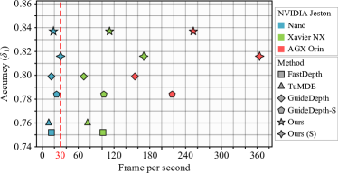
Figure 1: Accuracy (in $\delta_{1}$) vs. runtime (in FPS) on NVIDIA Jetson Nano, Xavier NX, and AGX Orin for various depth estimation algorithms on KITTI [9] dataset using the Eigen split [10]. The top right represents the desired characteristics of a depth estimation network design: high inference speed and high accuracy. The data comes from published papers or is measured using official implementation (online test, $batchsize=1$).

Considerable monocular depth estimation methods are proposed based on convolutional neural networks [11, 12, 13] and different types of supervision [14, 15, 16]. Current state-of-the-art monocular depth estimation CNN-based methods [17, 18, 19] have focused almost exclusively on pursuing accuracy, the resulting methods with intensive computation. Although these methods have significantly improved accuracy, the cost of doing so is increased by computational complexity and hardly deployed to resource-constrained embedded devices, which is still far from practical deployment. Most embedded systems are limited in computing resources and run multiple subtasks (e.g., object detection, depth estimation, and semantic segmentation) in parallel. To practical deployment of the monocular depth estimation in autonomous embedded systems, a key challenge is balancing the latency and the accuracy to enable real-time performance even with a limited computing budget.

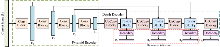
Figure 2: Proposed RT-MonoDepth framework. The shape of input image is $H\times W\times 3$, symbol ”F” denotes feature maps in the pyramid encoder, symbol ”D” denotes predicted depth maps in each scale, the subscript number indicates their shape (e.g., $F_{n}\colon\frac{H}{2^{n}}\times\frac{W}{2^{n}}\times C_{n}$, $D_{n}\colon\frac{H}{2^{n}}\times\frac{W}{2^{n}}\times 1$). Decoder₃, Decoder₂ and Decoder₁ can be removed when inferring.

Most recent works on efficient depth estimation approaches are devoted to improving the real-time performance of existing monocular depth estimation methods, focusing on the hardware-specific compilation [20], quantization [21], and model compression [22]. In addition, some works [23, 24] use the existing lightweight backbone design to achieve faster execution, while others [25] design an efficient decoding structure to reduce latency.

This paper presents a low latency, high-throughput, high-accuracy monocular depth estimation method running on embedded platforms. Our approach addresses the challenge of balancing the accuracy and the latency of monocular depth estimation of autonomous systems. We propose two efficient encoder-decoder network architectures, RT-MonoDepth and RT-MonoDepth-S, focusing on high-accuracy with medium-latency design and medium-accuracy with low-latency, respectively.

We analyze the delaying factors of signal stream, design a basic lightweight encoder-decoder architecture, explore the best parameter setting and feature fusion strategy, and obtain the final model. Our middle and low latency network design, RT-MonoDepth and RT-MonoDepth-S, can perform real-time depth estimation on the NVIDIA Jetson Nano, Xavier NX and AGX Orin without post-processing (e.g., network pruning, hardware optimization). Fig. 1 shows that our middle latency network design, RT-MonoDepth, can execute on the embedded platforms with reasonable accuracy and operate at over 253.0 frames per second (FPS) on the AGX Orin and around 18.4 FPS on the Nano. In addition, our small model, RT-MonoDepth-S, reaches solid performance at a high frame rate, operating at over 364.1 FPS on the AGX Orin and around 30.5 FPS on the Nano.

To sum up, we propose two lightweight convolutional neural networks for monocular depth estimation. To the best of the authors’ knowledge, our approach outperforms the related methods that target fast monocular depth estimation in terms of the best accuracy for the KITTI [9] benchmark while achieving the quickest inference speed.

II RELATED WORK

Depth sensing from a monocular camera has been an active topic in the research of computer vision and robotics communities for over a decade. Early works on depth estimation using single RGB images usually relied on probabilistic graphical models using hand-crafted features and non-parametric methods [26, 27, 28]. With the development of computer hardware and deep learning, the convolutional neural network has made significant progress in computer vision and robotics.

At first, Eigen et al. [10] proposed a coarse-to-fine network with two stacked sub-networks, one sub-network predicting the global coarse depth map and the other refining local details. Liu et al. [29] used a deep CNN and a continuous conditional random field (CRF) to jointly estimate depth from a single image and further improved depth estimation accuracy. In contrast, Laina et al. [11] suggested an end-to-end encoder-decoder architecture for monocular depth estimation, using a pre-trained ResNet [30] backbone as a feature extractor, and got comparable results to the depth sensor. Qi et al. [31] trained depth-to-normal and normal-to-depth networks to jointly estimate the depth and the surface normal maps to address the edge-blurring problem.

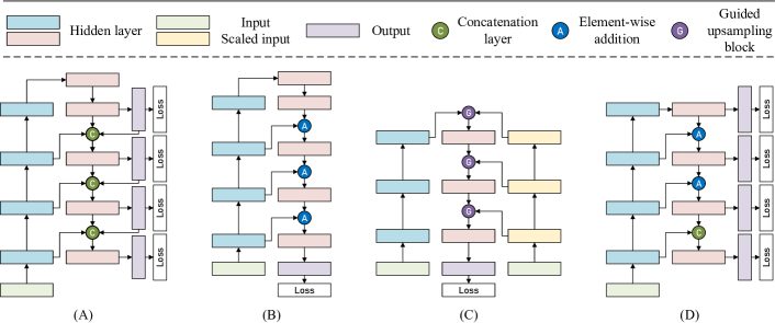
Figure 3: Feature fusion methods of different approaches. (A) Monodepth2 [32]; (B) FastDepth [23]; (C) GuideDepth [25]; (D) Our model.

Godard et al. [33] proposed an unsupervised training strategy using the left-right consistency of stereo pairs to solve the problem that CNN model training requires a large amount of labeled data. In contrast, Zhou et al. [34] suggested an unsupervised framework, solving the depth estimation problem as a view synthesis problem by combing the depth model with a pose model. Furthermore, Godard et al. [32] suggested a self-supervised strategy by applying auto-masking to the moving object and using novel minimum reprojection loss to improve the accuracy further, making Monodepth2 a monumental baseline model.

Most recently, state-of-the-art works significantly improved the accuracy of monocular depth estimation. Guizilini et al. [35] first introduced 3D convolution and used a novel symmetrical packing and unpacking block structure to learn the detail-preserving representations of depth estimation jointly. By employing the gated recurrent unit (GRU) and the convex upsampling module from RAFT [36], Zhou et al. [37] constructed a novel recurrent updates network to refine the prediction iteratively and achieved a high-level depth estimation performance. In contrast, Miangoleh et al. [19] suggested a double estimation method to merge low- and high-resolution predictions to achieve better performance both in the background and foreground. In the latest research, Yang et al. [18] proposed a transformer-based network with a unified attention gate structure, achieving the best monocular depth estimation accuracy.

Conversely, some works focus on finding the trade-off between accuracy and real-time performance. At first, Wofk et al. [23] proposed the FastDepth, an efficient method assembled by a pre-trained MobileNetV2 [38] backbone with a lightweight decoder. Tu et al. [24] designed a similar architecture but further simplified the decoder. To increase inference speed, Wofk et al. [23] and Tu et al. [24] compiled their models with TVM [20], and employed NetAdapt [22] and reinforcement learning algorithm [39] to reduce the model size, respectively. In the latest research, Rudolph et al. [25] proposed an efficient network, GuideDepth, conducted by a DDRNet-23-slim [40] backbone and a lightweight decoder with guided upsampling block. GuideDepth compared with Wofk et al. [23] and Tu et al. [24] in the condition without post-processing, and achieves the best result both in accuracy and inference speed on embedded platforms.

III METHOD

Our proposed fully convolutional encoder-decoder RT-MonoDepth framework is shown in Fig. 2. It consists of two pieces: a pyramid encoder and a depth decoder. The pyramid encoder extracts high-level low-resolution features from the input image. These feature maps are then transmitted into the depth decoder, where they are gradually upsampled, fused, and predicted the depth map at each scale. In designing a monocular depth estimation network that can run in real-time on embedded systems, we pursue low latency and high-precision designs for both the pyramid encoder and the depth decoder.

III-A Pyramid Encoder

The pyramid encoder usually employed a designed backbone network for image classification in past monocular depth estimation methods. ResNet [30] and MobileNet [38, 41] were the most common choices because of their powerful feature extraction ability and high accuracy. As a price of high performance, such structures are also subject to the limitations of complexity and latency, causing them to be deployed to resource-constrained embedded devices hardly. In addition, due to the fixed shape of the backbone network, it is also hard to design a flexible decoder for low latency.

Unlike previous monocular depth estimation methods, we construct a 4-layer pyramid encoder from scratch targeting low latency. Each layer has a ConvBlock, containing three $3\times 3$ convolution layers with activation functions. The ConvBlock downsample inputs and yields higher-level feature maps.

Due to the complex topologies and deep layers, ResNet and MobileNet insert the batch normalization layer [42] into the backbone to accelerate convergence. Considering that the capacity of GPU memory limits the dense regression task, a small batch size brings instability to the model using batch normalization [43]. Since we are committed to designing a simple, lightweight encoder, removing the normalization layer has no negative impact and can reduce computation slightly.

By instead standard convolution with depth-wise separable convolution, MobileNet dramatically reduces the computational complexity in theory. However, depth-wise convolution is slow in current deep learning frameworks while both training and inferring [44] because their implementations cannot fully utilize the GPU without hardware support. Thus, we only use standard convolutions in our framework to minimize latency.

TABLE I: Quantitative results of depth estimation on the KITTI dataset (Eigen split, 640$\times$192, 0-80m).

methods	year	Data	pre- train	#para  (M)	$\pagecolor{COLOR1}\mathrm{AbsRel}\downarrow$	$\pagecolor{COLOR1}\mathrm{SqRel}\downarrow$	$\pagecolor{COLOR1}\mathrm{RMSE}\downarrow$	$\pagecolor{COLOR1}\mathrm{RMSE_{log}}\downarrow$	$\pagecolor{COLOR2}\delta<1.25\uparrow$	$\pagecolor{COLOR2}\delta<1.25^{2}\uparrow$	$\pagecolor{COLOR2}\delta<1.25^{3}\uparrow$	FPS$\uparrow$  (Nano)	FPS$\uparrow$  (Xavier)	FPS$\uparrow$  (Orin)
FastDepth [23]	2019	D	$\bullet$	4.0	0.168	-	5.839	-	0.752	0.927	0.977	15.0	101.4	-
TuMDE [24]	2021	D	$\bullet$	5.7	0.150	-	5.801	-	0.760	0.930	0.980	10.5	75.7	-
GuideDepth [25]	2022	D	$\bullet$	5.8	0.142	-	5.194	-	0.799	0.941	0.982	15.2	69.3	155.0
GuideDepth-S [25]	2022	D	$\bullet$	5.7	0.142	-	5.480	-	0.784	0.936	0.981	25.2	102.9	217.5
Monodepth2 [32]	2019	M		14.3	0.132	1.044	5.142	0.210	0.845	0.948	0.977	-	-	142.3
Monodepth2 [32]	2019	M	$\bullet$	14.3	0.115	0.903	4.863	0.193	0.877	0.959	0.981	-	-	142.3
RT-MonoDepth(Ours)	-	M		2.8	0.125	0.959	4.985	0.202	0.857	0.952	0.979	18.4	112.5	253.0
RT-MonoDepth-S(Ours)	-	M		1.2	0.132	0.997	5.262	0.214	0.840	0.946	0.977	30.5	169.8	364.1
Monodepth2 [32]	2019	MS		14.3	0.127	1.031	5.266	0.221	0.836	0.943	0.974	-	-	142.3
Monodepth2 [32]	2019	MS	$\bullet$	14.3	0.106	0.818	4.750	0.196	0.874	0.957	0.979	-	-	142.3
RT-MonoDepth(Ours)	-	MS		2.8	0.127	0.995	5.153	0.217	0.837	0.944	0.975	18.4	112.5	253.0
RT-MonoDepth-S(Ours)	-	MS		1.2	0.135	1.040	5.413	0.229	0.816	0.936	0.973	30.5	169.8	364.1

III-B Depth Decoder

The function of the decoder is to upsample and fuse the output of the encoder to form a dense depth prediction. Determining how to design the three most critical parts of the depth decoder: upsampling layers, fusion layers, and prediction layers, to improve the throughput is the main objective.

Upsampling

Upsample operation is one of the basic designs of the low-latency depth decoder. In the past decades, many upsampling methods have been proposed (e.g., unpooling, transpose convolution, interpolation, interpolation combined with convolution). FastDepth [23] has explored the impact of different upsampling methods on depth performance. They compared the upsampling methods of different combinations and finally proposed an upsampling method called NNConv5 ($5\times 5$ depth-wise separable convolution followed by nearest-neighbor interpolation with a scale factor of $2$). We further instead NNConv5 with NNConv3 to achieve a faster inference speed. Each NNConv3 UpConvBlock performs $3\times 3$ standard convolution and reduces the number of output channels by 1/2 relative to the number of input channels, followed by nearest-neighbor interpolation that doubles the resolution of intermediate feature maps.

Fusion

Fusing the features of different scales is an essential means to improve performance in many works [45, 46]. The low-level features with high resolution have more spatial information but less semantic information and more noise. In contrast, the high-level features with low resolution have more semantic information but less spatial information. Two standard fusion methods in deep learning practice exist: element-wise addition and concatenate. Monodepth2 [32] gradually concatenates the upper-level feature maps to the lower level. Meanwhile, FastDepth [23] gradually adds the upper-level feature maps to the next level. In contrast, GuideDepth [25] introduces the guided upsampling block to use the input image as guidance to upsample the feature maps without previous level feature maps. To balance the latency and the accuracy, we perform element-wise addition at the first and second layers to accelerate feature fusion and concatenate at the third layer of the depth decoder for better final accuracy.

Prediction

Our model set one prediction decoder at each scale. Each decoder includes two $3\times 3$ convolution layers, followed by a leakyReLU and a sigmoid function as activating functions, respectively. Decoders receive the fused feature maps and yield depth prediction at each scale for self-supervision. We do not pass the intermediate depth prediction to the next level to minimize the latency, which allows us to disable the first three decoders to speed up inferencing.

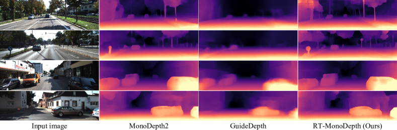
Figure 4: Qualitative results of monocular depth estimation comparing RT-MonoDepth with Monodepth2 and GuideDepth on the KITTI dataset. Our method provides cleaner boundaries and more effective object reconstruction than the other methods.

IV EXPERIMENT

In this section, we present experimental results to demonstrate our approach. We first introduce the details of our implementation. Then give an evaluation against existing high-precision or low-latency methods on the KITTI [9] benchmark for monocular depth estimation, and then provide ablation studies of our framework based on accuracy and latency metrics. Finally, we give some limitations and future directions of our approach.

IV-A Implementation details

Hardware Platforms

We train our networks at a single NVIDIA RTX 3090 GPU with a 9 GB GPU memory occupation. Then, we evaluate the real-time performance of our models on three edge computing embedded systems: NVIDIA Jetson Nano, Xavier NX, and AGX Orin. Nano and Xavier NX are low-power embedded devices, and the AGX Orin is the most powerful embedded platform deployed in autonomous systems. The Jetson Nano has a 4-core Arm Cortex-A57 processor, a 128-core NVIDIA Maxwell GPU, and 4 GB of RAM. The Jetson Xavier NX works with a 6-core NVIDIA Carmel Arm processor, a 384-core NVIDIA Volta GPU, and 8 GB of RAM. The AGX Orin owns a 12-core Arm Cortex-A78AE processor, a 2048-core NVIDIA Ampere GPU, and 32 GB of RAM. For a fair comparison, we report the results of Jetson Nano in 10W power mode and Jetson Xavier NX in 15W power mode, both of which use the same configurations described in [25]. In addition, we report detailed results run in AGX Orin to show our advantage compared with the state-of-the-art fast depth estimation method.

Dataset

We train and evaluate our networks on the KITTI [9] dataset using the train/test data split described in [10]. For training, we follow Zhou et al.’s [34] pre-processing to remove static frames. During the evaluation, we clip depth to 80m per standard practice [33].

Training Details

Our method is implemented in PyTorch [47] with 32-bit floating-point precision. We use the AdamW [48] optimizer with a learning rate of $1\times 10^{-4}$, and a batch size of 8. We train for 20 epochs and reduce the learning rate by 10 after 15 epochs. Additionally, we use the same data augmentation and the self-supervised strategy during training as Monodepth2 [32].

Testing Details

There are two standard testing methods in deep learning: offline and online. Offline testing is often used in some tasks without real-time requirements, allowing multiple data (batchsize=N) to be fed into the model for parallel processing. In contrast, online testing only allows one data (batchsize=1) to be sent into the model simultaneously to test the real-time performance. All inference speeds in our experiments were reported on models converted to TensorRT with 16-bit floating-point precision and online testing for a fair comparison. Unlike [25], we run each method 1000 times for a warm-up and then measure the time consumption with an average test time of 5000 iterations (10 warm-up and 200 testing in [25]).

Evaluation Metrics

We use standard six metrics used in used in prior work [32] to compare various methods. Let $\hat{d_{i}}$ be the pixel of prediction depth map $\hat{d}$, and $d_{i}$ be the pixel in the ground-truth $d$, and $N$ be the total number of pixels. Then we use the following evaluation metrics: absolute relative error ($\mathrm{AbsRel}$): $\frac{1}{N}\sum\frac{|d_{i}-\hat{d_{i}}|}{d_{i}}$; square relative error ($\mathrm{SqRel}$): $\frac{1}{N}\sum\frac{|d_{i}-\hat{d_{i}}|^{2}}{d_{i}}$; root mean square error ($\mathrm{RMSE}$): $\sqrt{\frac{1}{N}\sum{|d_{i}-\hat{d_{i}}|}^{2}}$; root mean square logarithmic error ($\mathrm{RMSE_{log}}$): $\sqrt{\frac{1}{N}\sum|\log_{10}d_{i}-\log_{10}\hat{d}_{i}|^{2}}$; threshold accuracy ($\delta_{j}$): $\%$ of $d_{i}$ s.t. $\max(\frac{d_{i}}{\hat{d_{i}}},\frac{\hat{d_{i}}}{d_{i}})=\delta<thr$ for $thr=1.25,1.25^{2},1.25^{3}$.

IV-B Final Results and Comparison With Prior Work

Results achieved with our methodology against some existing high-precision or low-latency methods are summarized in Table I. The symbol D in the Data column (data source used for training) refers to methods that use depth supervision at training time, M is for self-supervised training on monocular video, and MS is for models trained with stereo video. We also show results for Monodepth2 with ImageNet pretraining, denoted as the checkmark at the pre-train column.

We compare our model with some low-latency methods, e.g., FastDepth [23], TuMDE [24], and GuideDepth [25], and the classical method Monodepth2 [32]. We also evaluate a smaller model that reduces the running time by dropping the FusionBlock and reducing the layers of ConvBlock of the original version. The resulting model, RT-MonoDepth-S, is about 6% less accurate but 47% faster than RT-MonoDepth.

As shown in Table I, compared with the existing state-of-the-art low-latency method GuideDepth, RT-MonoDepth can perform about an average of 5% better than GuideDepth with 53% less parameter and an average of 60% higher FPS. For the lite version, RT-MonoDepth-S can perform about an average of 3% better than GuideDepth with 75% fewer parameters and an average of 63% higher FPS. Compared with the classical method Monodepth2, RT-MonoDepth can outperform Monodepth2 slightly without pre-training in all metrics. However, there is still a significant gap in performance between our method and the pre-trained Monodepth2.

As a result of our efficient, lightweight architecture design, the inference of RT-MonoDepth is possible with up to 18.4 FPS on the Jetson Nano and 253.0 FPS on the AGX Orin. For the lite version, RT-MonoDepth-S delivers up to 30.5 FPS on the NVIDIA Jetson Nano and up to 364.1 FPS on the AGX Orin. The low latency allows our methods can be directly deployed to the autonomous robot platform with high real-time performance requirements. To the best of our knowledge, our method is the fastest no-pruning monocular depth estimation method on embedded systems.

Qualitative results of our RT-MonoDepth, state-of-the-art fast monocular depth estimation method GuideDepth, and the classical method Monodepth2 (w/o pre-trained) are presented in Fig. 4. As shown in Fig. 4, our method performs better than GuideDepth obviously and can provide more effective object reconstruction than MonoDepth2, especially in the edge regions.

IV-C Ablation Studies

We explored the design space based on the RT-MonoDepth framework and conducted ablation studies on supervision scales, pyramid encoder levels, feature fusions, and other components and training strategies. All the ablation studies are performed with monocular and stereo self-supervision and tested on NVIDIA Jetson Nano at $640\times 192$ resolution.

Supervision scales

Monodepth2 [32], FastDepth [23], and GuideDepth [25] gradually merge feature maps in the decoder and output a full-resolution depth map at the last level. Monodepth2 [32] predicts depth maps and applies supervision signals at different scales, and these intermediate depth maps are merged upward and can not be ignored when inferencing. FastDepth [23] and GuideDepth [25] only yield depth maps at the last level and do not apply additional intermediate supervision signals. Table II summarizes the results of four variants that use 1, 2, 3, and 4 layers of supervision. The results show that deeper depth supervision leads to consistently better performance. Unlike Monodepth2, these intermediate predictions of RT-MonoDepth will not affect the final real-time performance because they can be ignored when inferencing.

TABLE II: Ablation experiments. Settings used in final model are bold.

Ablation	Parameter	$\pagecolor{COLOR1}\mathrm{AbsRel}\downarrow$	$\pagecolor{COLOR1}\mathrm{RMSE}\downarrow$	$\pagecolor{COLOR2}\delta<1.25\uparrow$	FPS$\uparrow$
Supervision Scales	1	0.128	5.227	0.834	18.4
	2	0.128	5.157	0.834	18.4
	3	0.128	5.158	0.836	18.4
	4	0.127	5.153	0.837	18.4
Encoder Levels	2	0.146	5.357	0.814	24.3
	3	0.133	5.207	0.828	20.9
	4	0.127	5.153	0.837	18.4
	5	0.123	5.080	0.837	16.2
Fusion Methods	+++	0.132	5.257	0.834	19.3
	++c	0.127	5.153	0.837	18.4
	+cc	0.126	5.139	0.837	17.6
	ccc	0.126	5.086	0.838	15.8

Feature Pyramid Levels

The feature pyramid levels determine the decoder’s starting minimum resolution, which is one of the critical parameters of such coarse-to-fine architecture. To fully use the employed backbone network, Monodepth2 [32] and FastDepth [23] extract the feature map with a minimum resolution of 1/32. In contrast, GuideDepth [25] only extracts the feature map with a minimum resolution of 1/8 to achieve a faster inference speed. Table II summarizes the results of four variants that use 2, 3, 4, and 5 layers of the feature pyramid, which extract the feature map with a minimum resolution of 1/4, 1/8, 1/16, and 1/32, respectively. The results show that more levels of the feature pyramid have higher precision but worse real-time performance. A pyramid level of 4 is a trade-off between accuracy and latency.

Feature Fusions

We tested the accuracy and latency of the model under different feature fusion methods. Table II summarizes the results of four methods that use different feature fusion methods. Symbol ’+’ refers to element-wise addition, and ’c’ is for concatenate. The results show that more concatenate operations have better precision but worse real-time performance. A method of ’++c’ is a trade-off between accuracy and latency.

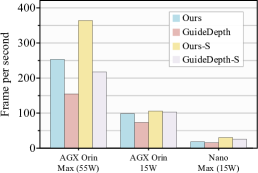
Figure 5: Comparison results of inferencing speed comparing RT-MonoDepth with GuideDepth. Our method provides faster inferencing speed than the GuideDepth.

IV-D Comparison of inferencing speed

We perform various speed tests of our RT-MonoDepth and the state-of-the-art fast monocular depth estimation method GuideDepth on the AGX Orin and Nano using the image resolution of 640$\times$192. The results are presented in Fig. 5. In the full power mode (Orin Max and Nano Max), our method is significantly faster than GuideDepth. With GPU improvement, our method’s advantages are more prominent. In addition, we make AGX Orin work in 15W mode to simulate the resource-constrained when a single device runs multiple tasks in parallel. The results show that our method is faster than GuideDepth, even under the condition of limited computing resources.

V LIMITATION

Table III shows the performance of RT-MonoDepth under different resolution inputs. Our method achieves promising results at low resolution. However, the performance of our approach is degraded when inputting high-resolution images. Our model trained with high-resolution images loses about 4% of the average performance compared with the low-resolution model. According to the existing research [49, 50, 19], the monocular depth estimation model mainly relies on the learned image edge features for depth estimation. High-resolution images will make the model need an encoder with a higher receptive field and complexity for effective learning. Our model uses a lightweight, simple encoder, which is challenging to learn accurately in high-resolution images, so the performance of our model degraded when training with high-resolution images.

TABLE III: Quantitative results of RT-MonoDepth with different resolution images on the KITTI dataset (Eigen split, 0-80m).

Resolution	Data	$\pagecolor{COLOR1}\mathrm{AbsRel}\downarrow$	$\pagecolor{COLOR1}\mathrm{RMSE}\downarrow$	$\pagecolor{COLOR2}\delta<1.25\uparrow$
640$\times$192	M	0.125	4.985	0.857
	MS	0.126	5.157	0.836
1024$\times$320	M	0.139	5.108	0.837
	MS	0.136	5.182	0.825

VI CONCLUSION

In this work, we design low latency monocular depth estimation networks on embedded systems for resource-constrained robot systems. We perform high frame rates by developing an efficient network architecture, referred to as RT-MonoDepth and RT-MonoDepth-S, with a low complexity and low-latency encoder-decoder design. On the Jetson Nano, Xavier NX, and AGX Orin, our final models achieve runtimes faster than prior works while maintaining comparable accuracy with related architectures on the KITTI dataset. To the best of our knowledge, our method is the fastest no-pruning monocular depth estimation method. We hope our methods can be a practical choice for real-world applications of autonomous driving and robotics. For future work, we aim to improve the accuracy of high-resolution input and further reduce the runtimes.

References

- [1] S. Wang, M. Mihajlovic, Q. Ma, A. Geiger, and S. Tang, “Metaavatar: Learning animatable clothed human models from few depth images,” in Advances in Neural Information Processing Systems (NeurIPS), pp. 2810–2822, 2021.
- [2] J. Wiederer, A. Bouazizi, U. Kressel, and V. Belagiannis, “Traffic control gesture recognition for autonomous vehicles,” in IEEE/RSJ International Conference on Intelligent Robots and Systems (IROS), pp. 10676–10683, 2020.
- [3] H. Mei, B. Dong, W. Dong, P. Peers, X. Yang, Q. Zhang, and X. Wei, “Depth-aware mirror segmentation,” in IEEE Conference on Computer Vision and Pattern Recognition (CVPR), pp. 3044–3053, 2021.
- [4] Y. Long, D. Morris, X. Liu, M. Castro, P. Chakravarty, and P. Narayanan, “Radar-camera pixel depth association for depth completion,” in IEEE Conference on Computer Vision and Pattern Recognition (CVPR), pp. 12507–12516, 2021.
- [5] M. Wei, D. Lee, V. Isler, and D. D. Lee, “Occupancy map inpainting for online robot navigation,” in IEEE International Conference on Robotics and Automation (ICRA), pp. 8551–8557, 2021.
- [6] P. Wenzel, T. Schön, L. Leal-Taixé, and D. Cremers, “Vision-based mobile robotics obstacle avoidance with deep reinforcement learning,” in IEEE International Conference on Robotics and Automation (ICRA), pp. 14360–14366, 2021.
- [7] J. Kopf, X. Rong, and J. Huang, “Robust consistent video depth estimation,” in IEEE Conference on Computer Vision and Pattern Recognition (CVPR), pp. 1611–1621, 2021.
- [8] X. Zuo, N. Merrill, W. Li, Y. Liu, M. Pollefeys, and G. Huang, “Codevio: Visual-inertial odometry with learned optimizable dense depth,” in IEEE International Conference on Robotics and Automation (ICRA), pp. 14382–14388, 2021.
- [9] A. Geiger, P. Lenz, C. Stiller, and R. Urtasun, “Vision meets robotics: The KITTI dataset,” Int. J. Robotics Res., vol. 32, no. 11, pp. 1231–1237, 2013.
- [10] D. Eigen, C. Puhrsch, and R. Fergus, “Depth map prediction from a single image using a multi-scale deep network,” in Advances in Neural Information Processing Systems (NeurIPS), pp. 2366–2374, 2014.
- [11] I. Laina, C. Rupprecht, V. Belagiannis, F. Tombari, and N. Navab, “Deeper depth prediction with fully convolutional residual networks,” in International Conference on 3D Vision (3DV), pp. 239–248, 2016.
- [12] D. Xu, W. Wang, H. Tang, H. Liu, N. Sebe, and E. Ricci, “Structured attention guided convolutional neural fields for monocular depth estimation,” in IEEE Conference on Computer Vision and Pattern Recognition (CVPR), pp. 3917–3925, 2018.
- [13] S. Gur and L. Wolf, “Single image depth estimation trained via depth from defocus cues,” in IEEE Conference on Computer Vision and Pattern Recognition (CVPR), pp. 7683–7692, 2019.
- [14] P. P. Srinivasan, R. Garg, N. Wadhwa, R. Ng, and J. T. Barron, “Aperture supervision for monocular depth estimation,” in IEEE Conference on Computer Vision and Pattern Recognition (CVPR), pp. 6393–6401, 2018.
- [15] K. Xian, C. Shen, Z. Cao, H. Lu, Y. Xiao, R. Li, and Z. Luo, “Monocular relative depth perception with web stereo data supervision,” in IEEE Conference on Computer Vision and Pattern Recognition (CVPR), pp. 311–320, 2018.
- [16] H. Zhan, R. Garg, C. S. Weerasekera, K. Li, H. Agarwal, and I. D. Reid, “Unsupervised learning of monocular depth estimation and visual odometry with deep feature reconstruction,” in IEEE Conference on Computer Vision and Pattern Recognition (CVPR), pp. 340–349, 2018.
- [17] V. Guizilini, R. Ambrus, S. Pillai, A. Raventos, and A. Gaidon, “3d packing for self-supervised monocular depth estimation,” in IEEE/CVF Conference on Computer Vision and Pattern Recognition (CVPR), pp. 2482–2491, 2020.
- [18] G. Yang, H. Tang, M. Ding, N. Sebe, and E. Ricci, “Transformer-based attention networks for continuous pixel-wise prediction,” in IEEE/CVF International Conference on Computer Vision (ICCV), pp. 16249–16259, 2021.
- [19] S. M. H. Miangoleh, S. Dille, L. Mai, S. Paris, and Y. Aksoy, “Boosting monocular depth estimation models to high-resolution via content-adaptive multi-resolution merging,” in IEEE Conference on Computer Vision and Pattern Recognition (CVPR), pp. 9685–9694, 2021.
- [20] T. Chen, T. Moreau, Z. Jiang, L. Zheng, E. Q. Yan, H. Shen, M. Cowan, L. Wang, Y. Hu, L. Ceze, C. Guestrin, and A. Krishnamurthy, “TVM: an automated end-to-end optimizing compiler for deep learning,” in USENIX Symposium on Operating Systems Design and Implementation (OSDI), pp. 578–594, 2018.
- [21] C. J. N. C. Jr., A. Kuusela, S. Li, H. Zhuang, J. Ngadiuba, T. K. Aarrestad, V. Loncar, M. Pierini, A. A. Pol, and S. Summers, “Automatic heterogeneous quantization of deep neural networks for low-latency inference on the edge for particle detectors,” Nat. Mach. Intell., vol. 3, no. 8, pp. 675–686, 2021.
- [22] T. Yang, A. G. Howard, B. Chen, X. Zhang, A. Go, M. Sandler, V. Sze, and H. Adam, “Netadapt: Platform-aware neural network adaptation for mobile applications,” in European Conference on Computer Vision (ECCV) (V. Ferrari, M. Hebert, C. Sminchisescu, and Y. Weiss, eds.), vol. 11214, pp. 289–304, 2018.
- [23] D. Wofk, F. Ma, T. Yang, S. Karaman, and V. Sze, “Fastdepth: Fast monocular depth estimation on embedded systems,” in International Conference on Robotics and Automation (ICRA), pp. 6101–6108, 2019.
- [24] X. Tu, C. Xu, S. Liu, R. Li, G. Xie, J. Huang, and L. T. Yang, “Efficient monocular depth estimation for edge devices in internet of things,” IEEE Trans. Ind. Informatics, vol. 17, no. 4, pp. 2821–2832, 2021.
- [25] M. Rudolph, Y. Dawoud, R. Güldenring, L. Nalpantidis, and V. Belagiannis, “Lightweight monocular depth estimation through guided decoding,” in IEEE International Conference on Robotics and Automation (ICRA), pp. 2344–2350, 2022.
- [26] A. Saxena, S. H. Chung, and A. Y. Ng, “Learning depth from single monocular images,” in Advances in Neural Information Processing Systems (NeurIPS), pp. 1161–1168, 2005.
- [27] K. Karsch, C. Liu, and S. B. Kang, “Depth extraction from video using non-parametric sampling,” in European Conference on Computer Vision (ECCV), vol. 7576, pp. 775–788, 2012.
- [28] K. Karsch, C. Liu, and S. B. Kang, “Depth transfer: Depth extraction from video using non-parametric sampling,” IEEE Trans. Pattern Anal. Mach. Intell., vol. 36, no. 11, pp. 2144–2158, 2014.
- [29] F. Liu, C. Shen, and G. Lin, “Deep convolutional neural fields for depth estimation from a single image,” in IEEE Conference on Computer Vision and Pattern Recognition (CVPR), pp. 5162–5170, 2015.
- [30] K. He, X. Zhang, S. Ren, and J. Sun, “Deep residual learning for image recognition,” in IEEE Conference on Computer Vision and Pattern Recognition (CVPR), pp. 770–778, 2016.
- [31] X. Qi, R. Liao, Z. Liu, R. Urtasun, and J. Jia, “Geonet: Geometric neural network for joint depth and surface normal estimation,” in IEEE Conference on Computer Vision and Pattern Recognition (CVPR), pp. 283–291, 2018.
- [32] C. Godard, O. M. Aodha, M. Firman, and G. J. Brostow, “Digging into self-supervised monocular depth estimation,” in IEEE/CVF International Conference on Computer Vision, ICCV, pp. 3827–3837, 2019.
- [33] C. Godard, O. M. Aodha, and G. J. Brostow, “Unsupervised monocular depth estimation with left-right consistency,” in IEEE Conference on Computer Vision and Pattern Recognition (CVPR), pp. 6602–6611, 2017.
- [34] T. Zhou, M. Brown, N. Snavely, and D. G. Lowe, “Unsupervised learning of depth and ego-motion from video,” in IEEE Conference on Computer Vision and Pattern Recognition (CVPR), pp. 6612–6619, 2017.
- [35] R. Ranftl, K. Lasinger, D. Hafner, K. Schindler, and V. Koltun, “Towards robust monocular depth estimation: Mixing datasets for zero-shot cross-dataset transfer,” IEEE Trans. Pattern Anal. Mach. Intell., vol. 44, no. 3, pp. 1623–1637, 2022.
- [36] Z. Teed and J. Deng, “RAFT: recurrent all-pairs field transforms for optical flow,” in European Conference on Computer Vision (ECCV) (A. Vedaldi, H. Bischof, T. Brox, and J. Frahm, eds.), vol. 12347, pp. 402–419, 2020.
- [37] Z. Zhou, X. Fan, P. Shi, and Y. Xin, “R-MSFM: recurrent multi-scale feature modulation for monocular depth estimating,” in IEEE/CVF International Conference on Computer Vision (ICCV), pp. 12757–12766, 2021.
- [38] M. Sandler, A. G. Howard, M. Zhu, A. Zhmoginov, and L. Chen, “Mobilenetv2: Inverted residuals and linear bottlenecks,” in IEEE Conference on Computer Vision and Pattern Recognition (CVPR), pp. 4510–4520, 2018.
- [39] Y. He, J. Lin, Z. Liu, H. Wang, L. Li, and S. Han, “AMC: automl for model compression and acceleration on mobile devices,” in European Conference on Computer Vision (ECCV), vol. 11211, pp. 815–832, 2018.
- [40] Y. Hong, H. Pan, W. Sun, and Y. Jia, “Deep dual-resolution networks for real-time and accurate semantic segmentation of road scenes,” arXiv preprint, arXiv:2101.06085,2021.
- [41] A. Howard, R. Pang, H. Adam, Q. V. Le, M. Sandler, B. Chen, W. Wang, L. Chen, M. Tan, G. Chu, V. Vasudevan, and Y. Zhu, “Searching for mobilenetv3,” in IEEE/CVF International Conference on Computer Vision (ICCV), pp. 1314–1324, 2019.
- [42] S. Ioffe and C. Szegedy, “Batch normalization: Accelerating deep network training by reducing internal covariate shift,” in International Conference on Machine Learning (ICML), vol. 37, pp. 448–456, 2015.
- [43] Y. Wu and K. He, “Group normalization,” in European Conference on Computer Vision (ECCV), vol. 11217, pp. 3–19, 2018.
- [44] Z. Qin, Z. Zhang, D. Li, Y. Zhang, and Y. Peng, “Diagonalwise refactorization: An efficient training method for depthwise convolutions,” in International Joint Conference on Neural Networks (IJCNN), pp. 1–8, 2018.
- [45] T. Lin, P. Dollár, R. B. Girshick, K. He, B. Hariharan, and S. J. Belongie, “Feature pyramid networks for object detection,” in IEEE Conference on Computer Vision and Pattern Recognition (CVPR), pp. 936–944, 2017.
- [46] Z. Zhang, X. Zhang, C. Peng, X. Xue, and J. Sun, “Exfuse: Enhancing feature fusion for semantic segmentation,” in European Conference on Computer Vision (ECCV), vol. 11214, pp. 273–288, 2018.
- [47] A. Paszke, S. Gross, F. Massa, A. Lerer, J. Bradbury, G. Chanan, T. Killeen, Z. Lin, N. Gimelshein, L. Antiga, A. Desmaison, A. Köpf, E. Z. Yang, Z. DeVito, M. Raison, A. Tejani, S. Chilamkurthy, B. Steiner, L. Fang, J. Bai, and S. Chintala, “Pytorch: An imperative style, high-performance deep learning library,” in Advances in Neural Information Processing Systems (NeurIPS), pp. 8024–8035, 2019.
- [48] I. Loshchilov and F. Hutter, “Decoupled weight decay regularization,” in International Conference on Learning Representations (ICLR), 2019.
- [49] J. Hu, Y. Zhang, and T. Okatani, “Visualization of convolutional neural networks for monocular depth estimation,” in IEEE/CVF International Conference on Computer Vision (ICCV), pp. 3868–3877, 2019.
- [50] X. Lyu, L. Liu, M. Wang, X. Kong, L. Liu, Y. Liu, X. Chen, and Y. Yuan, “Hr-depth: High resolution self-supervised monocular depth estimation,” in AAAI Conference on Artificial Intelligence, AAAI, pp. 2294–2301, 2021.