General procedure for free-surface recovery from bottom pressure measurements: Application to rotational overhanging waves

Abstract.

A novel boundary integral approach for the recovery of overhanging (or not) rotational (or not) water waves from pressure measurements at the bottom is presented. The method is based on the Cauchy integral formula and on an Eulerian–Lagrangian formalism to accommodate overturning free surfaces. This approach eliminates the need to introduce a priori a special basis of functions, providing thus a general means of fitting the pressure data and, consequently, recovering the free surface. The effectiveness and accuracy of the method are demonstrated through numerical examples.

1. Introduction

Nonlinear water waves have been extensively studied since the mid eighteenth century, when Euler introduced his eponymous equation. Since then, surface gravity waves have attracted much attention in their modelling, although scientists quickly realised their inherent complexity. This is one reason why physicists and mathematicians are still interested by the richness of this problem, making it an endless source for research in fluid dynamics. For instance, one crucial concern in environmental and coastal engineering is to accurately measure the surface of the sea for warning about the formation of large waves near coasts and oceanic routes. One solution to this problem is reconstructing the surface using a discrete set of measurements obtained from submerged pressure transducers [17]. This approach avoids the limitations of offshore buoy systems, which are susceptible to climatic disasters, located on moving boundaries, and lacking accuracy in wave height estimates [13]. Consequently, solving the nonlinear inverse problem associated with water-waves is a timely request for building practical engineering apparatus that rely on in situ data.

While the hydrostatic theory was originally used to tackle this problem when first formulated [1, 12], it was only recently that nonlinear waves began to be addressed [15]. Some works, such as [9], considered conformal mapping to successfully obtain reconstruction formulae. However, the numerical cost associated with solving these implicit relations renders conformal mapping inefficient when dealing with real physical data, i.e., when pressure data are given at known abscissas of the physical plane, not of the conformally mapped one. Actually, introducing some suitable holomorphic functions, it is possible to efficiently solve this nonlinear problem while staying within the physical plane for the recovery procedure [5, 3]. These studies demonstrated the convergence of the reconstruction process and the ability to recover waves of maximum amplitude [6]. Furthermore, the method was adapted to handle cases involving linear shear currents [7], remarkably recovering the unknown magnitude of vorticity alongside the wave profile and associated parameters.

The recovery method studied in [3, 5, 6, 7] has two shortcomings, however. First, it was developed for non-overhanging waves, so it cannot directly address these waves that can occur, in particular, in presence of vorticity. Second, part of this reconstruction procedure is based on analytic continuation of some well-chosen eigenfunctions. If for some waves a “good” choice of eigenfunctions is clear a priori, this is not necessarily the case for complicated wave profiles. By “good” choice, we mean a set of eigenfunctions that provides an accurate representation of the free surface with a minimal amount of modes and, at the same time, that can be easily computed. Even though Fourier series (or integrals) can be used in principle, a large number of eigenfunctions may be required to accurately represent the free surface. Since a surface recovery from bottom pressure is intrinsically ill-conditioned, using a large number of Fourier modes may lead to numerical issues. Another basis should then be preferably employed. For instance, for irrotational long waves propagating in shallow water (i.e., cnoidal waves), the use of Jacobian elliptic functions is effective [3, 5]. However, such alternative basis are not always easily guessed. Thus, it is desirable to derive a reconstruction procedure independent of a peculiar basis of eigenfunctions. Here, we propose a recovery methodology addressing these two shortcoming.

In this article, we derive a general formulation to address the surface recovery problem using a boundary integral formulation. While a similar approach was described by Da Silva and Peregrine [11] for computing rotational waves, to our knowledge it has never been applied in the context of a recovery procedure. The Cauchy integral formula, although singular by definition, proves advantageous from a numerical perspective. Dealing with singular kernels, the integral formulation easily allows for the consideration of arbitrary steady rotational surface waves (periodic, solitary, aperiodic) without the need to select a peculiar basis of functions to fit the pressure data. Additionally, this method facilitates the parametrisation of the surface profile, enabling the recovery of overhanging waves with arbitrarily large amplitudes.

Overturning profiles are known to be hard to compute accurately [18], which presents a significant challenge due to the ill-posed nature of our problem. Nevertheless, by considering a mixed Eulerian–Lagrangian description at the boundaries, we demonstrate the feasibility of the recovery process. To illustrate the robustness of our method, we present two examples of rotational steady waves: a periodic wave with an overturning surface and a solitary wave. In both scenarii, we achieve good agreement in recovering the wave elevation, albeit with the necessity of using refined grids in the regions of greatest surface variation. Refining a grid where needed is way much easier than finding a better basis of functions, that is a feature of considerable practical interest.

The method presented in this study consists in the first boundary integral approach to solve this nonlinear recovery problem. We expect this work to pave the way for addressing even more challenging configurations, including the extension to three-dimensional settings, which will inevitably involve Green functions in the integral kernels.

The paper is organised as follow. The mathematical model and relations of interest are introduced in section 2, with an Eulerian description of motion. In order to handle overhanging waves, their Lagrangian counterparts are introduced in section 4. In section 3, we derive an equation for the free surface, allowing us to compute reference solutions for testing our recovery procedure. This procedure is described in the subsequent section 5. Numerical implementation and examples are provided in section 6. Finally, in section 7, we discuss our general results, as well as the future extensions and implications of this work.

2. Mathematical settings

We give here the classical formulation of our water-wave problem in Eulerian variables. Physical assumptions and notations being identical to that of Clamond et al. [7], interested readers should refer to this paper for further details.

2.1. Equations of motion and useful relations

We consider the steady two-dimensional motion of an incompressible inviscid fluid with constant vorticity $\omega$. The fluid is bounded above and below by impermeable free surface and solid horizontal bed, respectively. Our focus lies on traveling waves of permanent form that propagate with a constant phase speed $c$ and wavenumber $k$ ($k=0$ for solitary and more general aperiodic waves). We adopt a Galilean frame of reference moving with the wave, thus ensuring that the velocity field appears independent of time for the observer. Consequently, we can express the fluid domain, denoted as $\Omega$, as the set of points $(x,y)$ (Cartesian coordinates) satisfying $x\in\mathds{R}$ and $-0pt\leqslant y\leqslant\eta(x)$, where $\eta(x)$ represents the surface elevation from rest and $0pt$ is the mean water depth. Thus, the mean water level is located at $y=0$, such that

$$\langle\eta\rangle\stackrel{{\scriptstyle\text{\tiny{def}}}}{{=}}\frac{k}{2\pi}\int_{-\pi/k}^{\pi/k}\eta(x)\mathrm{d}x=0,$$ (1)

where $\langle\bm{\cdot}\rangle$ denotes the Eulerian averaging operator (c.f. Figure 1).

In this setting, the velocity field $\bm{u}=(u,v)$ and pressure $p$ (divided by the density and relative to the reference value at the surface) are governed by the stationary Euler equations

$$\bm{\nabla}\bm{\cdot}\bm{u}=0,\qquad\bm{u}\bm{\cdot}\bm{\nabla}\bm{u}+\bm{\nabla}p+\bm{g}=0,$$

where $\bm{g}=(0,g)$, the acceleration due to gravity $g>0$ acting downwards. Equations of motion ($(2a,b)$) are supplemented with kinematic and dynamic conditions at the upper and lower boundaries

$$\bm{u}\bm{\cdot}\bm{n}-\bm{u}\bm{\cdot}\bm{\nabla}\eta =0\quad\textrm{at}\quad y=\eta(x),$$ (3a)

$$p =0\quad\textrm{at}\quad y=\eta(x),$$ (3b)

$$\bm{u}\bm{\cdot}\bm{n} =0\quad\textrm{at}\quad y=-d,$$ (3c)

where $\bm{n}$ is the outward normal vector (see Figure 1 for a sketch of this configuration).

Since our physical system is two-dimensional per se, we introduce a scalar stream function $\psi$ such that $u=\psi_{y}$ and $v=-\psi_{x}$, so ($(2a,b)$a) is satisfied identically and $\omega=-\psi_{xx}-\psi_{yy}$ is assumed constant. Thus, the Euler equations can be integrated into the Bernoulli equation

$$2(p+gy)+u^{2}+v^{2}={B}_{\mathrm{s}}-2\omega(\psi-{\psi}_{\mathrm{s}})\stackrel{{\scriptstyle\text{\tiny{def}}}}{{=}}B(\psi),$$ (4)

for a constant ${B}_{\mathrm{s}}$ [7]. Alternatively, we can define a Bernoulli constant at the bottom ${B}_{\mathrm{b}}\stackrel{{\scriptstyle\text{\tiny{def}}}}{{=}}{B}_{\mathrm{s}}-2\omega({\psi}_{\mathrm{b}}-{\psi}_{\mathrm{s}})$. In (4), as in the rest of the article, subscripts ‘s’ and ‘b’ denote that the fields are evaluated, respectively, at the surface and at the bottom. The free surface and the seabed being both streamlines, ${\psi}_{\mathrm{s}}$ and ${\psi}_{\mathrm{b}}$ are constant in this problem.

Because here ${p}_{\mathrm{s}}=0$ (constant atmospheric pressure set to zero without loss of generality), we have the relations relating some average bottom quantities and parameters [7]

$$\left<\/{p}_{\mathrm{b}}\/\right>=g0pt,\qquad\left<\/{u}_{\mathrm{b}}^{\,2}\/\right>={B}_{\mathrm{b}},\qquad\left<\/{u}_{\mathrm{b}}-\left(1+\eta_{x}^{\,2}\right){u}_{\mathrm{s}}\/\right>=\omega\/0pt.$$

Although we decide to set the reference frame as moving with the wave celerity, it is still useful to consider Stokes’ first and second definitions of phase speed

$$c_{1} \stackrel{{\scriptstyle\text{\tiny{def}}}}{{=}}-\left<{u}_{\mathrm{b}}\right>=-\omega 0pt-\left<\left(1+\eta_{x}^{2}\right){u}_{\mathrm{s}}\right>,$$ (6)

$$c_{2} \stackrel{{\scriptstyle\text{\tiny{def}}}}{{=}}-\left<\frac{1}{0pt}\int_{-0pt}^{\eta}u\mathrm{d}y\right>=\frac{{\psi}_{\mathrm{b}}-{\psi}_{\mathrm{s}}}{0pt}=-\frac{\omega 0pt}{2}-\frac{\omega\left<\eta^{2}\right>}{20pt}-\frac{\left<\left(1+\eta_{x}^{2}\right)h\,{u}_{\mathrm{s}}\right>}{0pt},$$ (7)

where $h\stackrel{{\scriptstyle\text{\tiny{def}}}}{{=}}\eta(x)+0pt$ is the local water depth.

Figure 1. Definition sketch in the referential moving with the wave.

2.2. Holomorphic functions

The vorticity being constant, potential theory still holds when using a Helmholtz representation to subtract the contribution of the linear shear current [7]. Therefore, it is convenient to introduce the complex relative velocity

$$W(z)\stackrel{{\scriptstyle\text{\tiny{def}}}}{{=}}U(x,y)-\mathrm{i}V(x,y)=(y+0pt)\omega+u(x,y)-\mathrm{i}v(x,y),$$ (8)

that is holomorphic in $\Omega$ for the complex coordinate $z\stackrel{{\scriptstyle\text{\tiny{def}}}}{{=}}x+\mathrm{i}y$. (Obviously, the complex velocity $w\stackrel{{\scriptstyle\text{\tiny{def}}}}{{=}}u-\mathrm{i}v$ is not holomorphic if $\omega\neq 0$.) The relative complex velocity (8) is related to the relative complex potential $F(z)\stackrel{{\scriptstyle\text{\tiny{def}}}}{{=}}\Phi(x,y)+\mathrm{i}\Psi(x,y)$ by $W=\mathrm{d}F/\mathrm{d}z$, where $U=\Phi_{x}=\Psi_{y}$ and $V=\Phi_{y}=-\Psi_{x}$ (see Clamond et al. [7] for more details).

Following Clamond and Constantin [5], we introduce a complex “pressure” function as

$${\mathfrak{P}}(z)\/\stackrel{{\scriptstyle\text{\tiny{def}}}}{{=}}\/g0pt+{\textstyle{\frac{1}{2}}}{B}_{\mathrm{s}}+\omega({\psi}_{\mathrm{s}}-{\psi}_{\mathrm{b}})-{\textstyle{\frac{1}{2}}}W(z)^{2}=g0pt+{\textstyle{\frac{1}{2}}}{B}_{\mathrm{b}}-{\textstyle{\frac{1}{2}}}W(z)^{2},$$ (9)

that is holomorphic in the fluid domain $\Omega$, its restriction to the flat bed $y=-0pt$ having zero imaginary part and real part $p_{\text{b}}$. Thus, $p_{\text{b}}$ determines $\mathfrak{P}$ uniquely throughout the fluid domain, i.e., ${\mathfrak{P}}(z)={p}_{\mathrm{b}}(z+\mathrm{i}0pt)$. Note that $p$ introduced in ($(2a,b)$) coincides with the real part of $\mathfrak{P}$ only on $y=-0pt$ because the former is not a harmonic function in the fluid domain [8, 10].

As for irrotational waves, it is useful [3, 4, 7] to introduce the anti-derivative of $\mathfrak{P}(z)$

$$\mathfrak{Q}(z)\stackrel{{\scriptstyle\text{\tiny{def}}}}{{=}}\int_{z_{0}}^{z}\left[\mathfrak{P}(z^{\prime})-g0pt\right]\mathrm{d}z^{\prime}=\int_{z_{0}}^{z}{\textstyle{\frac{1}{2}}}\left[{B}_{\mathrm{b}}-W(z^{\prime})^{2}\right]\mathrm{d}z^{\prime},$$ (10)

where $z_{0}$ is an arbitrary constant. For the same abscissa $x$, the functions $\mathfrak{Q}$ at the free surface (i.e., ${\mathfrak{Q}}_{\mathrm{s}}(x)$) and at the bottom (i.e., ${\mathfrak{Q}}_{\mathrm{b}}(x)$) satisfy the relation

$${\mathfrak{Q}}_{\mathrm{s}}(x)-{\mathfrak{Q}}_{\mathrm{b}}(x)=\int_{x-\mathrm{i}d}^{x+\mathrm{i}\eta(x)}\left[\/\mathfrak{P}(z)-g0pt\/\right]\mathrm{d}z=\frac{\mathrm{i}h(x){B}_{\mathrm{b}}}{2}-\int_{x-\mathrm{i}d}^{x+\mathrm{i}\eta(x)}\frac{W(z)^{2}}{2}\mathrm{d}z.$$ (11)

2.3. Cauchy integral formula

In the complex $z$-plane, the boundaries are analytical curves defined by ${z}_{\mathrm{s}}=x+\mathrm{i}\eta$ and ${z}_{\mathrm{b}}=x-\mathrm{i}d$. For a holomorphic function $\Upxi(z)$, the Cauchy integral formula applied to the fluid domain $\Omega$ (assuming non-intersecting and non-overturning seabed and free surface) yields

$$\mathrm{i}\vartheta\,\Upxi(z)=\text{P.V.}\oint\frac{\Upxi(z^{\prime})}{z^{\prime}-z}\mathrm{d}z^{\prime}=\int_{-\infty}^{\infty}\frac{{\Upxi}_{\mathrm{b}}^{\prime}\mathrm{d}x^{\prime}}{{z}_{\mathrm{b}}^{\prime}-z}-\int_{-\infty}^{\infty}\frac{\left(1+\mathrm{i}\eta_{x}^{\prime}\right){\Upxi}_{\mathrm{s}}^{\prime}\mathrm{d}x^{\prime}}{{z}_{\mathrm{s}}^{\prime}-z},$$ (12)

where $\vartheta=\{2\pi,0,\pi\}$ respectively inside, outside and at the smooth boundary of the domain. We emphasis that, in this paper, all integrals must be taken in the sense of the Cauchy principal value (P.V.), even if it is not explicitly mentioned for brevity. When $\operatorname{Im}\{{\Upxi}_{\mathrm{b}}\}=0$, the bottom boundary condition can be taken into account with the method of images, yielding

$$\Upxi(z)=\frac{\mathrm{i}}{\vartheta}\int_{-\infty}^{\infty}\frac{\left(1+\mathrm{i}\eta_{x}^{\prime}\right){\Upxi}_{\mathrm{s}}^{\prime}\mathrm{d}x^{\prime}}{{z}_{\mathrm{s}}^{\prime}-z}-\frac{\mathrm{i}}{\vartheta}\int_{-\infty}^{\infty}\frac{\left(1-\mathrm{i}\eta_{x}^{\prime}\right){\bar{\Upxi}}_{\mathrm{s}}^{\prime}\mathrm{d}x^{\prime}}{{\bar{z}}_{\mathrm{s}}^{\prime}-z-2\mathrm{i}d},$$ (13)

where an overbar denotes the complex conjugation. Note that the formula (13) is valid in finite depth (provided that $\operatorname{Im}\{{\Upxi}_{\mathrm{b}}\}=0$), and in infinite depth if ${\Upxi}_{\mathrm{b}}\to 0$ as $d\to\infty$. Examples of functions satisfying these conditions are $\Upxi=W+c_{1}$, $\Upxi=W^{2}-{B}_{\mathrm{b}}$ and $\Upxi=\mathfrak{P}-gd$, so (13) provides an expression for computing these functions in arbitrary depth.

2.4. Integral formulations for periodic waves

For $L$-periodic waves (with $L=2\pi/k$), the kernel is repeated in the horizontal direction, along the interval $\mathcal{I}=[0,L]$, leading to the Cauchy integral formula with Hilbert kernel

$$\Upxi(z)=\frac{\mathrm{i}k}{2\vartheta}\int_{\mathcal{I}}\left[\cot\!\left(k\frac{{z}_{\mathrm{s}}^{\prime}-z}{2}\right)\left(1+\mathrm{i}\eta_{x}^{\prime}\right){\Upxi}_{\mathrm{s}}^{\prime}-\cot\!\left(k\frac{{z}_{\mathrm{b}}^{\prime}-z}{2}\right){\Upxi}_{\mathrm{b}}^{\prime}\right]\mathrm{d}x^{\prime}.$$ (14)

Alternatively, using the method of images, along with the identity (65), the Cauchy integral can be written

$$\Upxi(z)=\frac{k}{\vartheta}\int_{\mathcal{I}} \left[\mbox{\,L{\scriptsize{i}}}_{0}\{\mathrm{e}^{\mathrm{i}k({z}_{\mathrm{s}}^{\prime}-z)}\}\left(1+\mathrm{i}\eta_{x}^{\prime}\right){\Upxi}_{\mathrm{s}}^{\prime}+\mbox{\,L{\scriptsize{i}}}_{0}\{\mathrm{e}^{\mathrm{i}k(z-{\bar{z}}_{\mathrm{s}}^{\prime}+2\mathrm{i}0pt)}\}\left(1-\mathrm{i}\eta_{x}^{\prime}\right){\bar{\Upxi}}_{\mathrm{s}}\right]\mathrm{d}x^{\prime}$$

$$+\pi\/\vartheta^{-1}\langle\/(1+\mathrm{i}\eta_{x}){\Upxi}_{\mathrm{s}}+(1-\mathrm{i}\eta_{x}){\bar{\Upxi}}_{\mathrm{s}}\rangle,$$ (15)

where $\mbox{\,L{\scriptsize{i}}}_{\nu}$ is the $\nu$th polylogarithm whose definition is given in appendix A along with useful relations. It is worth noticing that the last term in the right-hand side of (2.4) corresponds to the zeroth Fourier coefficient (not present when the holomorphic function $\Upxi(z)$ has zero mean over the wave period). Equation (2.4) can be rewritten using the identity (64), yielding

$$\Upxi(z)=\frac{\mathrm{i}}{\vartheta}\int_{\mathcal{I}}\frac{\partial}{\partial\/z} \left[\mbox{\,L{\scriptsize{i}}}_{1}\{\mathrm{e}^{\mathrm{i}k({z}_{\mathrm{s}}^{\prime}-z)}\}\left(1+\mathrm{i}\eta_{x}^{\prime}\right){\Upxi}_{\mathrm{s}}^{\prime}-\mbox{\,L{\scriptsize{i}}}_{1}\{\mathrm{e}^{\mathrm{i}k(z-{\bar{z}}_{\mathrm{s}}^{\prime}+2\mathrm{i}0pt)}\}\left(1-\mathrm{i}\eta_{x}^{\prime}\right){\bar{\Upxi}}_{\mathrm{s}}\right]\mathrm{d}\/x^{\prime}$$

$$+2\/\pi\/\vartheta^{-1}\left<\operatorname{Re}{\left\{{\Upxi}_{\mathrm{s}}\right\}}-\eta_{x}\operatorname{Im}{\left\{{\Upxi}_{\mathrm{s}}\right\}}\right>,$$ (16)

At the free surface (where $\vartheta=\pi$, $z={z}_{\mathrm{s}}$ and $\mathrm{d}{z}_{\mathrm{s}}=(1+\mathrm{i}\eta_{x})\mathrm{d}\/x$), carefully applying the Leibniz integral rule (c.f. formula (71) in appendix B) on the singular term in the integrand, equation (2.4) reduces to

$$\left(1+\mathrm{i}\eta_{x}\right){\Upxi}_{\mathrm{s}}= \frac{\mathrm{i}}{2\pi}\frac{\mathrm{d}}{\mathrm{d}\/x}\int_{\mathcal{I}}\left[\mbox{\,L{\scriptsize{i}}}_{1}\{\mathrm{e}^{\mathrm{i}k({z}_{\mathrm{s}}^{\prime}-{z}_{\mathrm{s}})}\}\left(1+\mathrm{i}\eta_{x}^{\prime}\right){\Upxi}_{\mathrm{s}}^{\prime}-\mbox{\,L{\scriptsize{i}}}_{1}\{\mathrm{e}^{\mathrm{i}k({z}_{\mathrm{s}}-{\bar{z}}_{\mathrm{s}}^{\prime}+2\mathrm{i}0pt)}\}\left(1-\mathrm{i}\eta_{x}^{\prime}\right){\bar{\Upxi}}_{\mathrm{s}}\right]\mathrm{d}\/x^{\prime}$$

$$+\left(1+\mathrm{i}\eta_{x}\right)\left<\operatorname{Re}{\left\{{\Upxi}_{\mathrm{s}}\right\}}-\eta_{x}\operatorname{Im}{\left\{{\Upxi}_{\mathrm{s}}\right\}}\right>.$$ (17)

It should be noted that, obviously, aperiodic equations can be obtained from the periodic ones letting $L\to\infty$ (i.e. $k\to 0^{+}$). Thus, for now on, we only consider periodic waves.

3. Lagrangian description

This section focuses on addressing the limitation of the Eulerian framework that hinders the computation of overhanging waves, which are characterised by multi-valued surfaces. While one option to address this challenge involves employing an arclength formulation, as elaborated by Vanden-Broeck [18], we have chosen to adopt a Lagrangian formalism in this study. One benefit of the Lagrangian approach is its inherent capability to aggregate collocation points near the wave crest, where they are most crucial [11].

Our approach is similar to that used by Da Silva and Peregrine [11], although we modify the integral kernels in terms of polylogarithms and we primitive the Cauchy integral formula to remove the strong singularity from the kernels following Clamond [4]. The resulting analytical expression is characterised by a weak logarithmic singularity, and it is suitable for calculating various types of waves, including solitary and periodic waves, overhanging or not.

Considering the (rotational) complex velocity $w=u-\mathrm{i}v$ evaluated at the surface, let introduce the holomorphic function $\log{(-{w}/\sqrt{gd})}={q}-\mathrm{i}{\theta}$ and define accordingly

$${q}_{\mathrm{s}} \stackrel{{\scriptstyle\text{\tiny{def}}}}{{=}}\operatorname{Re}{\{\log{(-{w}_{\mathrm{s}}/\sqrt{gd})}\}}=\frac{1}{2}\ln{\left[({u}_{\mathrm{s}}^{2}+{v}_{\mathrm{s}}^{2})/\sqrt{gd}\right]},$$

$${\theta}_{\mathrm{s}} \stackrel{{\scriptstyle\text{\tiny{def}}}}{{=}}-\operatorname{Im}{\{\log{(-{w}_{\mathrm{s}}/\sqrt{gd})}\}}=-\operatorname{atan2}{({v}_{\mathrm{s}},-{u}_{\mathrm{s}})},$$ (18)

where we notably used the Bernoulli’s principle at the surface.

Exploiting the impermeability and isobarity of the free surface, one gets

$$\tan{{\theta}_{\mathrm{s}}}=\eta_{x}=\frac{{v}_{\mathrm{s}}}{{u}_{\mathrm{s}}}=\frac{\sigma{v}_{\mathrm{s}}}{\sqrt{{B}_{\mathrm{s}}-2g\eta-{v}_{\mathrm{s}}^{2}}}=\frac{\sqrt{{B}_{\mathrm{s}}-2g\eta-{u}_{\mathrm{s}}^{2}}}{\sigma{u}_{\mathrm{s}}}.$$ (19)

Hence, extracting ${u}_{\mathrm{s}}$ and ${v}_{\mathrm{s}}$ from the latter relations, we have

$${u}_{\mathrm{s}}=\sigma\cos({{\theta}_{\mathrm{s}}})\sqrt{{B}_{\mathrm{s}}-2g\eta},\quad{v}_{\mathrm{s}}=\sigma\sin({{\theta}_{\mathrm{s}}})\sqrt{{B}_{\mathrm{s}}-2g\eta}.$$ (20)

We now consider the Lagrangian description of motion, with $t$ denoting the time, thus ${u}_{\mathrm{s}}=\mathrm{d}x/\mathrm{d}t$ and ${v}_{\mathrm{s}}=\mathrm{d}\eta/\mathrm{d}t$ ($\mathrm{d}/\mathrm{d}t$ the temporal derivative following the motion). From the second expression in (20), we deduce that

$$\frac{\mathrm{d}}{\mathrm{d}t}\sqrt{{B}_{\mathrm{s}}-2g\eta}=-\sigma g\sin({{\theta}_{\mathrm{s}}}),$$ (21)

and hence, considering a crest at $t=0$ (where $\eta(0)=a$ is the wave amplitude), we have

$$\sqrt{{B}_{\mathrm{s}}-2g\eta}=\mu-g\sigma\int_{0}^{t}\sin({{\theta}_{\mathrm{s}}^{\prime}})\,\mathrm{d}t^{\prime},\quad\mu\stackrel{{\scriptstyle\text{\tiny{def}}}}{{=}}\sqrt{{B}_{\mathrm{s}}-2ga},$$ (22)

where ${\theta}_{\mathrm{s}}^{\prime}\stackrel{{\scriptstyle\text{\tiny{def}}}}{{=}}{\theta}_{\mathrm{s}}(t^{\prime})$. Therefore, all quantities at the free surface can be expressed in terms of the surface angle ${\theta}_{\mathrm{s}}$, using $t$ as independent variable, e.g.

$${z}_{\mathrm{s}}(t) =\sigma\int_{0}^{t}\left[\mu-g\sigma\int_{0}^{t^{\prime}}\sin({{\theta}_{\mathrm{s}}^{\prime\prime}})\,\mathrm{d}t^{\prime\prime}\right]\exp{(\mathrm{i}{\theta}_{\mathrm{s}}^{\prime})}\mathrm{d}t^{\prime}+\mathrm{i}a,$$ (23)

$${w}_{\mathrm{s}}(t) =\frac{\mathrm{d}{\bar{z}}_{\mathrm{s}}}{\mathrm{d}t}=\sigma\left[\mu-g\sigma\int_{0}^{t}\sin({\theta}_{\mathrm{s}}^{\prime})\,\mathrm{d}t^{\prime}\right]\exp{(-\mathrm{i}{\theta}_{\mathrm{s}})},$$ (24)

$$\eta(t) =\operatorname{Im}{{z}_{\mathrm{s}}}=\frac{{B}_{\mathrm{s}}}{2g}-\frac{1}{2g}\left[\mu-g\sigma\int_{0}^{t}\sin({\theta}_{\mathrm{s}}^{\prime})\,\mathrm{d}t^{\prime}\right]^{2}.$$ (25)

In the Eulerian description of motion, the wave period is constant and depends on the reference frame (moving at a constant phase speed) where one observes the fluid. On the other hand, in the Lagrangian context, the period $T_{L}$ of the free surface differs from the Eulerian period due to the Stokes drift [14]. The Lagrangian period being such that $\eta(t+T_{L})=\eta(t)$, we exploit expression (25) which, after some elementary algebra and simplifications, yields

$$\left[2\mu-g\sigma\int_{t}^{t+T_{L}}\sin({\theta}_{\mathrm{s}}^{\prime})\,\mathrm{d}t^{\prime}-2g\sigma\int_{0}^{t}\sin({\theta}_{\mathrm{s}}^{\prime})\,\mathrm{d}t^{\prime}\right]\int_{t}^{t+T_{L}}\sin({\theta}_{\mathrm{s}}^{\prime})\,\mathrm{d}t^{\prime}=0,$$ (26)

that is necessarily satisfied for all times if and only if

$$\int_{0}^{T_{L}}\sin({\theta}_{\mathrm{s}}^{\prime})\,\mathrm{d}t^{\prime}=0,$$ (27)

thus defining the Lagrangian period $T_{L}$.

4. Equations for the free surface

Since we do not have access to measurements of the bottom pressure for rotational waves, we must generate these data from numerical solutions of the exact equations. Thus, this section aims to derive a comprehensive formulation for the computation of surface wave using a boundary integral method. From these solutions, the bottom pressure is subsequently obtained and used as input for our surface recovery procedure.

4.1. Eulerian formulation

From expressions (4) and (8), the complex (irrotational part of the) velocity at the surface is given explicitly by

$${W}_{\mathrm{s}}=\omega h+\sigma\left(1-\mathrm{i}\eta_{x}\right)\sqrt{({B}_{\mathrm{s}}-2g\eta)/(1+\eta_{x}^{2})},$$ (28)

$\sigma=\mp 1$ denoting waves propagating upstream or downstream, respectively. The parameter $\sigma$ is introduced for convenience in order to characterise the (arbitrarily chosen) direction of the wave propagation in a ‘fixed’ frame of reference, i.e., $\sigma=-1$ if the wave travels toward the increasing $x$-direction in this frame and, obviously, $\sigma=+1$ if the wave travels toward the decreasing $x$-direction.

Considering the holomorphic function $\Upxi=W+c$ ($c$ being an arbitrary definition of the phase speed), the left-hand side of (2.4) follows directly from (28)

$$\left(1+\mathrm{i}\eta_{x}\right){\Upxi}_{\mathrm{s}}=\left(\omega h+c\right)\left(1+\mathrm{i}\eta_{x}\right)+\sigma\sqrt{({B}_{\mathrm{s}}-2g\eta)(1+\eta_{x}^{2})},$$ (29)

where the radicand is purely real since ${B}_{\mathrm{s}}\geqslant\max(2g\eta)$ for all waves. Substituting expression (29) in (2.4), the integral term splits into several contributions as

$$\omega\eta\left(1+\mathrm{i}\eta_{x}\right)= \frac{\mathrm{i}}{2\pi}\frac{\mathrm{d}}{\mathrm{d}\/x}\left[\int_{\mathcal{C}}\mbox{\,L{\scriptsize{i}}}_{1}\{\mathrm{e}^{\mathrm{i}k({z}_{\mathrm{s}}^{\prime}-{z}_{\mathrm{s}})}\}\left(\omega h^{\prime}+c\right)\mathrm{d}{z}_{\mathrm{s}}^{\prime}+\int_{\mathcal{C}}\mbox{\,L{\scriptsize{i}}}_{1}\{\mathrm{e}^{\mathrm{i}k({z}_{\mathrm{s}}-{\bar{z}}_{\mathrm{s}}^{\prime}+2\mathrm{i}0pt)}\}\left(\omega h^{\prime}+c\right)\mathrm{d}{\bar{z}}_{\mathrm{s}}^{\prime}\right.$$

$$+\left.\sigma\int_{\mathcal{I}}\mbox{\,L{\scriptsize{i}}}_{\nu}\!\left(\mathrm{e}^{\mathrm{i}k({z}_{\mathrm{s}}^{\prime}-{z}_{\mathrm{s}})}\right)-\mbox{\,L{\scriptsize{i}}}_{\nu}\!\left(\mathrm{e}^{\mathrm{i}k({z}_{\mathrm{s}}-{\bar{z}}_{\mathrm{s}}^{\prime}+2\mathrm{i}0pt)}\right)\sqrt{({B}_{\mathrm{s}}-2g\eta)(1+\eta_{x}^{2})}\mathrm{d}x^{\prime}\right]$$

$$+\left(1+\mathrm{i}\eta_{x}\right)\langle{u}_{\mathrm{s}}\left(1+\eta_{x}^{2}\right)\rangle-\sigma\sqrt{({B}_{\mathrm{s}}-2g\eta)(1+\eta_{x}^{2})},$$ (30)

where $\mathcal{C}$ represents the free surface path, i.e., we use the brief notations $\int_{\mathcal{C}}(\cdots)\/\mathrm{d}{z}_{\mathrm{s}}^{\prime}\stackrel{{\scriptstyle\text{\tiny{def}}}}{{=}}\int_{\mathcal{I}}(\cdots)(1+\mathrm{i}\eta_{x}^{\prime})\/\mathrm{d}\/x^{\prime}$ and $\int_{\mathcal{I}}(\cdots)\/\mathrm{d}\/x^{\prime}\stackrel{{\scriptstyle\text{\tiny{def}}}}{{=}}\int_{0}^{L}(\cdots)\/\mathrm{d}\/x^{\prime}$. The first term inside the square bracket of the right-hand side of (4.1) reduces to

$$J_{1} \stackrel{{\scriptstyle\text{\tiny{def}}}}{{=}}\int_{\mathcal{C}}\mbox{\,L{\scriptsize{i}}}_{1}\!\left(\mathrm{e}^{\mathrm{i}k({z}_{\mathrm{s}}^{\prime}-{z}_{\mathrm{s}})}\right)(\omega h^{\prime}+c)\,\mathrm{d}\/{z}_{\mathrm{s}}^{\prime}=\omega\int_{\mathcal{C}}\mbox{\,L{\scriptsize{i}}}_{1}\!\left(\mathrm{e}^{\mathrm{i}k({z}_{\mathrm{s}}^{\prime}-{z}_{\mathrm{s}})}\right)\eta^{\prime}\,\mathrm{d}\/{z}_{\mathrm{s}}^{\prime}$$

$$=\omega\int_{\mathcal{I}}\mbox{\,L{\scriptsize{i}}}_{1}\!\left(\mathrm{e}^{\mathrm{i}k({z}_{\mathrm{s}}^{\prime}-{z}_{\mathrm{s}})}\right)\eta^{\prime}\left(1+\mathrm{i}\eta_{x}^{\prime}\right)\mathrm{d}\/x^{\prime}=\frac{\mathrm{i}\omega}{k}\int_{\mathcal{I}}\mbox{\,L{\scriptsize{i}}}_{2}\!\left(\mathrm{e}^{\mathrm{i}k({z}_{\mathrm{s}}^{\prime}-{z}_{\mathrm{s}})}\right)\eta_{x}^{\prime}\,\mathrm{d}\/x^{\prime}$$

$$=-\frac{\omega}{k}\int_{\mathcal{I}}\mbox{\,L{\scriptsize{i}}}_{2}\!\left(\mathrm{e}^{\mathrm{i}k({z}_{\mathrm{s}}^{\prime}-{z}_{\mathrm{s}})}\right)\mathrm{d}\/x^{\prime},$$

where we exploited the property [4]

$$\int_{\mathcal{C}}\mbox{\,L{\scriptsize{i}}}_{\nu}\!\left(\mathrm{e}^{\mathrm{i}k{z}_{\mathrm{s}}}\right)\mathrm{d}{z}_{\mathrm{s}}=0.$$ (31)

Similarly, we have

$$J_{2}\stackrel{{\scriptstyle\text{\tiny{def}}}}{{=}}\int_{\mathcal{C}}\mbox{\,L{\scriptsize{i}}}_{1}\!\left(\mathrm{e}^{\mathrm{i}k({z}_{\mathrm{s}}-{\bar{z}}_{\mathrm{s}}^{\prime}+2\mathrm{i}0pt)}\right)(\omega h^{\prime}+c)\,\mathrm{d}\/{\bar{z}}_{\mathrm{s}}^{\prime}=-\frac{\omega}{k}\int_{\mathcal{I}}\mbox{\,L{\scriptsize{i}}}_{2}\!\left(\mathrm{e}^{\mathrm{i}k({z}_{\mathrm{s}}-{\bar{z}}_{\mathrm{s}}^{\prime}+2\mathrm{i}0pt)}\right)\mathrm{d}\/x^{\prime}.$$ (32)

Finally, after integrating the whole expression (4.1) and retaining the imaginary part only, we obtain the equation for the free surface

$$K= \,\frac{\omega\/\eta^{2}}{2}-\eta\left<{u}_{\mathrm{s}}(1+\eta_{x}^{2})\right>+\frac{\omega}{2\pi k}\int_{\mathcal{I}}\operatorname{Re}\{\mathcal{L}_{2}\}\,\mathrm{d}\/x^{\prime}$$

$$\,-\frac{\sigma}{2\pi}\int_{\mathcal{I}}\operatorname{Re}\{\mathcal{L}_{1}\}\sqrt{({B}_{\mathrm{s}}-2g\eta^{\prime})(1+\eta_{x}^{\prime 2})}\,\mathrm{d}\/x^{\prime},$$ (33)

where $K$ is an integration constant obtained enforcing the mean-level condition (1), i.e,

$$K=\left<\frac{\omega\eta^{2}}{2}+\frac{\omega}{2\pi k}\int_{\mathcal{I}}\operatorname{Re}\{\mathcal{L}_{2}\}\,\mathrm{d}\/x^{\prime}\,-\frac{\sigma}{2\pi}\int_{\mathcal{I}}\operatorname{Re}\{\mathcal{L}_{1}\}\sqrt{({B}_{\mathrm{s}}-2g\eta^{\prime})(1+\eta_{x}^{\prime 2})}\,\mathrm{d}\/x^{\prime}\right>.$$ (34)

From now on, the same notation $K$ is used to denote integration constants in the different surface recovery formulas. The exact values of these constants is obtained, as above, enforcing the condition (1). Moreover, we have introduced, for brevity, the notation for the kernels

$$\mathcal{L}_{\nu}\stackrel{{\scriptstyle\text{\tiny{def}}}}{{=}}\mbox{\,L{\scriptsize{i}}}_{\nu}\!\left(\mathrm{e}^{\mathrm{i}k({z}_{\mathrm{s}}^{\prime}-{z}_{\mathrm{s}})}\right)-\mbox{\,L{\scriptsize{i}}}_{\nu}\!\left(\mathrm{e}^{\mathrm{i}k({z}_{\mathrm{s}}-{\bar{z}}_{\mathrm{s}}^{\prime}+2\mathrm{i}0pt)}\right).$$ (35)

Equation (33) is a nonlinear integro-differential equation for the computation of the surface elevation $\eta$. Once $\eta$ is obtained solving (33) numerically, one can compute the corresponding bottom pressure. This bottom pressure can then be considered as “experimental data” to illustrate the reconstruction procedure described below. This is necessary when such data are not available from physical measurement, as it is the case with rotational waves.

4.2. Lagrangian formulation

Expression (27) provides an implicit definition of $T_{L}$ if the wavelength $L$ is fixed a priori. It is now of interest to convert our formula for the surface elevation (33) using the Lagrangian description introduced previously (the variable of interest now becomes ${\theta}_{\mathrm{s}}$). After some simplifications, we obtain

$$\frac{\omega\sigma}{2} \eta^{2}-\frac{k\eta}{2\pi}\int_{0}^{T_{L}}({B}_{\mathrm{s}}-2g\eta)\mathrm{d}t-\frac{1}{2\pi}\int_{0}^{T_{L}}\operatorname{Re}{\{\mathcal{L}_{1}\}}({B}_{\mathrm{s}}-2g\eta^{\prime})\mathrm{d}t^{\prime}$$

$$+\frac{\omega\sigma}{2\pi k}\int_{0}^{T_{L}}\operatorname{Re}{\{\mathcal{L}_{2}\}}\cos\!\left({{\theta}_{\mathrm{s}}^{\prime}}\right)\sqrt{{B}_{\mathrm{s}}-2g\eta^{\prime}}\,\mathrm{d}t^{\prime}=K,$$ (36)

where $K$ is recovered using condition (1) in the same way as to obtain (34).

The computation of (36) involves weak logarithmic singularities in the kernel of the $\mathcal{L}_{1}$ operator. In the numerical implementation, we use a similar approach as the one presented by Clamond [4], by subtracting the regular part of the operator. Thence, we obtain an explicit expression for the regularized finite integral as

$$\int_{0}^{T_{L}}\operatorname{Re}{\{\mathcal{L}_{1}\}}({B}_{\mathrm{s}}-2g\eta^{\prime})\mathrm{d}t^{\prime}= -2g\int_{0}^{T_{L}}\operatorname{Re}{\{\mathcal{L}_{1}\}}(\eta^{\prime}-\eta)\mathrm{d}t^{\prime}$$

$$+({B}_{\mathrm{s}}-2g\eta)\int_{0}^{T_{L}}\operatorname{Re}{\{\mathcal{L}_{1}-\widehat{\mathcal{L}}_{1}\}}\mathrm{d}t^{\prime},$$ (37)

where we introduced

$$\widehat{\mathcal{L}}_{\nu}\stackrel{{\scriptstyle\text{\tiny{def}}}}{{=}}\mbox{\,L{\scriptsize{i}}}_{\nu}\{\mathrm{e}^{\mathrm{i}\tau(t^{\prime}-t)}\}-\mbox{\,L{\scriptsize{i}}}_{\nu}\{\mathrm{e}^{\mathrm{i}\tau(t-t^{\prime})}\mathrm{e}^{-2k0pt}\},$$ (38)

with $\tau\stackrel{{\scriptstyle\text{\tiny{def}}}}{{=}}2\pi/T_{L}$. Considering $t\to t^{\prime}$ in both integrands in (4.2), we have

$$\lim_{t\to t^{\prime}}\operatorname{Re}{\{\mathcal{L}_{1}\}}(\eta-\eta^{\prime}) =0,$$ (39)

$$\lim_{t\to t^{\prime}}\operatorname{Re}{\{\mathcal{L}_{1}-\widehat{\mathcal{L}}_{1}\}} =\log\!\left[\left(\frac{1-\mathrm{e}^{-2kh}}{1-\mathrm{e}^{-2k0pt}}\right)\frac{\tau/k}{\sqrt{{B}_{\mathrm{s}}-2g\eta}}\right].$$ (40)

The numerical computation of Lagrangian surface waves is thus done by solving the nonlinear expression (36), providing a given wave amplitude $\left.\eta\right|_{t=0}=a$. The wave period $T_{L}$, as well as the Bernoulli constant $B_{s}$, are both obtained from the Lagrangian counterpart of (1) and the requirement that $\int_{0}^{T_{L}}\mathrm{d}{z}_{\mathrm{s}}=2\pi\sigma/k$. Moreover, since the abscissa $x(t)$ is given explicitly from the definition of the wave profile $\eta(t)$ through the real part of formula (23), we only have to solve expression (36) for $\eta$ — and not for both $x$ and $\eta$, as done previously by Da Silva and Peregrine [11] and by Vanden-Broeck [18] — thus allowing us to further reduce the numerical cost.

5. Surface recovery from bottom pressure

Building upon the last three sections, we propose a nonlinear integral equation to recover the surface elevation in terms of a given measure of pressure ${p}_{\mathrm{b}}(x)$ at the seabed. This ‘measurement’ is given here numerically by solving expression (36) and, subsequently, computing the pressure from the surface profile (exploiting the boundary integrals and the Bernoulli equation).

The principal benefit in establishing an integral formulation lies in the fact that no specific eigenfunctions are needed to fit the pressure data. In fact, our derived equation remains applicable regardless of the nature of the wave under consideration, be it periodic or not, overhanging or not. We reemphasise here that, although the equations consider $(2\pi/k)$-periodic waves, their aperiodic counterparts are easily obtained letting $k\to 0^{+}$.

5.1. Eulerian boundary integral formulation

Let consider the Cauchy integral formula (2.4) (without the method of images) for the holomorphic function $\Upxi(z)=\mathfrak{P}(z)-g0pt$. It yields

$$\mathfrak{P}-g0pt= \frac{k}{\vartheta}\int_{\mathcal{I}}\left[\mbox{\,L{\scriptsize{i}}}_{0}\!\left(\mathrm{e}^{\mathrm{i}k({z}_{\mathrm{s}}^{\prime}-z)}\right)(1+\mathrm{i}\eta_{x}^{\prime})({\mathfrak{P}}_{\mathrm{s}}^{\prime}-g0pt)-\mbox{\,L{\scriptsize{i}}}_{0}\!\left(\mathrm{e}^{\mathrm{i}k({z}_{\mathrm{b}}^{\prime}-z)}\right)({\mathfrak{P}}_{\mathrm{b}}^{\prime}-g0pt)\right]\mathrm{d}x^{\prime}$$

$$+\langle(1+\mathrm{i}\eta_{x})({\mathfrak{P}}_{\mathrm{s}}-g0pt)-({\mathfrak{P}}_{\mathrm{b}}^{\prime}-g0pt)\rangle.$$ (41)

In order to simplify the latter expression, we exploit both definitions of ${\mathfrak{P}}_{\mathrm{b}}\stackrel{{\scriptstyle\text{\tiny{def}}}}{{=}}p_{b}(x)$ and $\mathrm{d}{\mathfrak{Q}}_{\mathrm{s}}/\mathrm{d}x=({\mathfrak{P}}_{\mathrm{s}}-g0pt)(1+\mathrm{i}\eta_{x})$ (we recall that ${\mathfrak{Q}}_{\mathrm{s}}$ is a periodic function). Hence, expression (5.1) can be rewritten

$$\mathfrak{P}-g0pt=\frac{\mathrm{i}}{\vartheta}\int_{\mathcal{I}}\frac{\partial}{\partial z}\left[\mbox{\,L{\scriptsize{i}}}_{1}\!\left(\mathrm{e}^{\mathrm{i}k({z}_{\mathrm{s}}^{\prime}-z)}\right)(1+\mathrm{i}\eta_{x}^{\prime})({\mathfrak{P}}_{\mathrm{s}}^{\prime}-g0pt)-\mbox{\,L{\scriptsize{i}}}_{1}\!\left(\mathrm{e}^{\mathrm{i}k({z}_{\mathrm{b}}^{\prime}-z)}\right)({p}_{\mathrm{b}}^{\prime}-g0pt)\right]\mathrm{d}x^{\prime}.$$ (42)

Before pursuing, let introduce the compact notations for the polylogarithmic kernels

$$\mathcal{K}_{\nu}\stackrel{{\scriptstyle\text{\tiny{def}}}}{{=}}\mbox{\,L{\scriptsize{i}}}_{\nu}\!\left(\mathrm{e}^{\mathrm{i}k({z}_{\mathrm{s}}^{\prime}-{z}_{\mathrm{s}})}\right)\quad\textrm{and}\quad\mathcal{J}_{\nu}\stackrel{{\scriptstyle\text{\tiny{def}}}}{{=}}\mbox{\,L{\scriptsize{i}}}_{\nu}\!\left(\mathrm{e}^{\mathrm{i}k({z}_{\mathrm{b}}^{\prime}-{z}_{\mathrm{s}})}\right).$$ (43)

We now evaluate expression (42) at the free surface, reducing it to

$$({\mathfrak{P}}_{\mathrm{s}}-g0pt)(1+\mathrm{i}\eta_{x})=\frac{\mathrm{i}}{2\pi}\frac{\mathrm{d}}{\mathrm{d}x}\int_{\mathcal{I}}\left[\mathcal{K}_{1}(1+\mathrm{i}\eta_{x}^{\prime})({\mathfrak{P}}_{\mathrm{s}}^{\prime}-g0pt)-\mathcal{J}_{1}({\mathfrak{P}}_{\mathrm{b}}^{\prime}-g0pt)\right]\mathrm{d}x^{\prime}.$$ (44)

As one can notice, the left-hand side of (44) is the integrand of ${\mathfrak{Q}}_{\mathrm{s}}$. For that reason, we first integrate the whole expression over the $x$-coordinate and then split the contributions from the surface and the bottom

$${\mathfrak{Q}}_{\mathrm{s}}=\frac{\mathrm{i}}{2\pi}\int_{\mathcal{I}}\mathcal{K}_{1}(1+\mathrm{i}\eta_{x}^{\prime})({\mathfrak{P}}_{\mathrm{s}}^{\prime}-g0pt)\mathrm{d}x^{\prime}-\frac{\mathrm{i}}{2\pi}\int_{\mathcal{I}}\mathcal{J}_{1}({p}_{\mathrm{b}}^{\prime}-g0pt)\mathrm{d}x^{\prime}+K,$$ (45)

for a constant of integration $K$ also obtained applying condition (1).

The next step is to decompose the integrand in the first integral of (45). To do so, we merely replace the complex velocity by its expression (8) and exploit the identity (31) to cancel out some constant terms, i.e.

$$\int_{\mathcal{C}}\mathcal{K}_{1}({\mathfrak{P}}_{\mathrm{s}}^{\prime}-g0pt)\mathrm{d}{z}_{\mathrm{s}}^{\prime} = -\frac{1}{2}\int_{\mathcal{C}}\mathcal{K}_{1}{W}_{\mathrm{s}}^{\prime 2}\mathrm{d}{z}_{\mathrm{s}}^{\prime}=-\frac{1}{2}\int_{\mathcal{C}}\mathcal{K}_{1}\left[\omega h^{\prime}+(1-\mathrm{i}\eta_{x}^{\prime})\sqrt{\frac{({B}_{\mathrm{s}}-2g\eta^{\prime})}{(1+\eta_{x}^{\prime 2})}}\right]^{2}\mathrm{d}{z}_{\mathrm{s}}^{\prime}$$

$$= -\frac{\omega^{2}}{2}\int_{\mathcal{C}}\mathcal{K}_{1}h^{\prime 2}\mathrm{d}{z}_{\mathrm{s}}^{\prime}-\omega\sigma\int_{\mathcal{C}}\mathcal{K}_{1}h^{\prime}(1-\mathrm{i}\eta_{x}^{\prime})\sqrt{\frac{({B}_{\mathrm{s}}-2g\eta^{\prime})}{(1+\eta_{x}^{\prime 2})}}\mathrm{d}{z}_{\mathrm{s}}^{\prime}$$

$$-\frac{1}{2}\int_{\mathcal{C}}\mathcal{K}_{1}(1-\mathrm{i}\eta_{x}^{\prime})^{2}\frac{({B}_{\mathrm{s}}-2g\eta^{\prime})}{(1+\eta_{x}^{\prime 2})}\mathrm{d}{z}_{\mathrm{s}}^{\prime}.$$ (46)

After some algebraic manipulations, it further reduces to

$$\int_{\mathcal{C}}\mathcal{K}_{1}({\mathfrak{P}}_{\mathrm{s}}^{\prime}-g0pt)\mathrm{d}{z}_{\mathrm{s}}^{\prime} = -\frac{\omega^{2}}{2}\int_{\mathcal{C}}\mathcal{K}_{1}\eta^{\prime 2}\mathrm{d}{z}_{\mathrm{s}}^{\prime}-\omega^{2}0pt\int_{\mathcal{C}}\mathcal{K}_{1}\eta^{\prime}\mathrm{d}{z}_{\mathrm{s}}^{\prime}$$

$$-\frac{1}{2}\int_{\mathcal{I}}\mathcal{K}_{1}({B}_{\mathrm{s}}-2g\eta^{\prime})(1-\mathrm{i}\eta_{x}^{\prime})\mathrm{d}x^{\prime}$$

$$-\omega\sigma\int_{\mathcal{I}}\mathcal{K}_{1}h^{\prime}\sqrt{({B}_{\mathrm{s}}-2g\eta^{\prime})(1+\eta_{x}^{\prime 2})}\mathrm{d}x^{\prime}$$

$$= -\frac{\mathrm{i}\omega^{2}}{k}\int_{\mathcal{I}}\mathcal{K}_{2}\eta^{\prime}\eta_{x}^{\prime}\mathrm{d}x^{\prime}+\frac{\omega^{2}0pt+g}{k}\int_{\mathcal{I}}\mathcal{K}_{2}\mathrm{d}x^{\prime}$$

$$-\int_{\mathcal{I}}\mathcal{K}_{1}({B}_{\mathrm{s}}-2g\eta^{\prime})\mathrm{d}x^{\prime}$$

$$-\omega\sigma\int_{\mathcal{I}}\mathcal{K}_{1}h^{\prime}\sqrt{({B}_{\mathrm{s}}-2g\eta^{\prime})(1+\eta_{x}^{\prime 2})}\mathrm{d}x^{\prime}.$$ (47)

Substituting (5.1) into (45), the imaginary part yields the Eulerian integral formulation for the surface recovery

$$2\pi\operatorname{Im}\{{\mathfrak{Q}}_{\mathrm{s}}\}= \frac{\omega^{2}}{2k}\int_{\mathcal{I}}\operatorname{Im}\{\mathcal{K}_{2}\}(\eta^{\prime 2})_{x}\mathrm{d}x^{\prime}-\int_{\mathcal{I}}\operatorname{Re}\{\mathcal{K}_{1}\}({B}_{\mathrm{s}}-2g\eta^{\prime})\mathrm{d}x^{\prime}$$

$$+\frac{\omega^{2}0pt+g}{k}\int_{\mathcal{I}}\operatorname{Re}\{\mathcal{K}_{2}\}\mathrm{d}x^{\prime}-\int_{\mathcal{I}}\operatorname{Re}\{\mathcal{J}_{1}\}({\mathfrak{P}}_{\mathrm{b}}^{\prime}-g0pt)\mathrm{d}x^{\prime}$$

$$-\omega\sigma\int_{\mathcal{I}}\operatorname{Re}\{\mathcal{K}_{1}\}h^{\prime}\sqrt{({B}_{\mathrm{s}}-2g\eta^{\prime})(1+\eta_{x}^{\prime 2})}\mathrm{d}x^{\prime}-2\pi\operatorname{Im}\{K\},$$ (48)

where $K$ is the same constant as in (45).

Equation (5.1) is a nonlinear integral equations for the free surface recovery from the bottom pressure. Being strictly Eulerian, this equation is not suitable for overhanging waves. For the latter, one can proceed as follow.

5.2. Hybrid formulation

Equation (5.1) involves integrals at the free surface and at the bottom. In practice, the bottom pressure is given at some known abscissa $x$, so the bottom integral must be kept in Eulerian form. However, Eulerian integrals are not suitable for overhanging waves, so we rewrite surface integrals in their Lagrangian counterparts. Doing so, the inverse problem is described by a mixed Eulerian–Lagrangian formalism.

Thus, the surface integrals in (5.1) being rewritten in Lagrangian description, the bottom integral being kept in Eulerian form, one gets the general expression for the surface recovery

$$2\pi\operatorname{Im}\{{\mathfrak{Q}}_{\mathrm{s}}\}= \frac{\omega^{2}}{k}\int_{0}^{T_{L}}\left[k^{-1}\operatorname{Re}\{\mathcal{K}_{3}\}+\left(h^{\prime}+g\omega^{-2}\right)\operatorname{Re}\{\mathcal{K}_{2}\}\right]\cos({\theta}_{\mathrm{s}}^{\prime})\sqrt{{B}_{\mathrm{s}}-2g\eta^{\prime}}\mathrm{d}t^{\prime}$$

$$-\int_{0}^{T_{L}}\operatorname{Re}\{\mathcal{K}_{1}\}\left[\cos({\theta}_{\mathrm{s}}^{\prime})\sqrt{{B}_{\mathrm{s}}-2g\eta^{\prime}}+\sigma\omega h^{\prime}\right]\left({B}_{\mathrm{s}}-2g\eta^{\prime}\right)\mathrm{d}t^{\prime}$$

$$-\int_{0}^{L}\operatorname{Re}\{\mathcal{J}_{1}\}({p}_{\mathrm{b}}^{\prime}-g0pt)\mathrm{d}x^{\prime}-2\pi\operatorname{Im}\{K\}.$$ (49)

This reformulation is necessary for practical recovery of overhanging waves. It is of course also suitable for non-overhanging waves.

6. Numerical illustrations

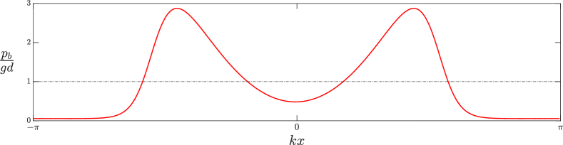
(a)

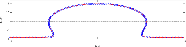
(b)

Figure 2. Numerical demonstration of the surface recovery procedure for an overhanging and periodic steady wave with a constant vorticity $\omega\sqrt{d/g}=3\sqrt{2}$. (a) Eulerian representation of the bottom pressure. The dashed dot line corresponds to the mean bottom pressure. (b) Surface wave profile (blue circles) obtained from expression (33). The red line represents the surface reconstruction achieved from ${p}_{\mathrm{b}}$ through equation (5.2), while the dashed dot line indicates the mean water level.

6.1. Details on the overall methodology

From a numerical standpoint, the nonlinear integral equations (33) and (5.2), employed respectively for computing the surface profile and recovering it from the bottom pressure, possess notable characteristics. First, these equations eliminate the need for evaluating the derivative of ${\theta}_{\mathrm{s}}$ at any point. Second, we can rely on Fourier analysis since the kernels are periodic and use trapezoidal rule for numerical integration.

Since we already know the value of $g$ and the wavenumber $k$ (or equivalently the wave period $L$) as inputs in our numerical scheme, we can deduce the depth of the layer $d$ from the definition of the hydrostatic law [3, 7]. For simplicity, we consider that the constant vorticity $\omega$ is known. However, $\omega$ can also be determined adapting the procedure described by Clamond et al. [7]. Then, initialising our numerical schemes with an appropriate initial guess, either from linear theory or by a previous iteration, as done by Da Silva and Peregrine [11], we observe fast convergence for a discrete set of $N$ equidistant points. In our simulations, we typically use $N=128$ for moderate waves and $N=512$ for waves (regardless of whether they exhibit overturning or not) with large amplitudes.

When investigating overhanging waves, the non-algebraic nonlinearities inherent in the problem often pose numerical challenges. The most troublesome issue arises from aliasing errors present in the functions spectra, a phenomenon occasionally referred to as “spectral blocking” [2], leading to exponential growth of high frequencies. As a consequence, this aliasing effect prevent the spectral accuracy inherent in our formulation. To address this issue, we employ the “zero padding” method, which involves increasing the size of the quadrature in Fourier space while appending zeros above the Nyquist frequency. Subsequently, we transform the functions back to physical space, compute the nonlinear terms, and filter out the previously introduced zero frequencies from the spectrum. For quadratic nonlinear terms, enlarging the degree of quadrature by a factor of $3/2$ has proven sufficient to mitigate this phenomenon [16]. However, in the context of non-algebraic nonlinearities encountered in this study, this argument does not hold, and the exact value of the enlargement factor remains unknown. Instead, we utilize a factor of $2$ (typically suitable for cubic nonlinearities) when performing products throughout the algorithm. Although we experimented with larger factors in our simulations, it appeared that this value was adequate for eliminating spurious frequencies in most aliased spectra.

In addition to aliasing, we noticed that it is numerically more efficient to perform a change of coordinates in evaluating the finite integrals. Particularly, significant variations in ${\theta}_{\mathrm{s}}$ occur where the wave undergoes overturning, indicating a requirement for additional collocation points in these regions. Thus, rather than evaluating the previous integrals with respect to the time variable $t\in[0,T_{L}]$, we introduce a new integration variable $\Upxi(t)$, defined as

$$\frac{\mathrm{d}\xi}{\mathrm{d}t}\stackrel{{\scriptstyle\text{\tiny{def}}}}{{=}}\sqrt{1+\beta\sin\!\left({\theta}_{\mathrm{s}}\right)^{2}},$$ (50)

where $\beta$ is a scaling parameter arbitrarily set. A similar change of coordinate can be found in [11]. In most simulations involving overhanging waves, we employ a value of $\beta=2\pi/(kdN)$.

Finally, we solve the whole system of equations (33) and (5.2) with the built-in iterative solver fsolve from Matlab software, using the Levenberg–Marquardt algorithm.

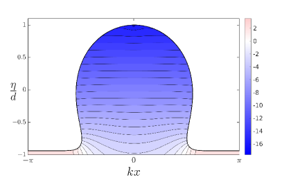
(a)

(b)

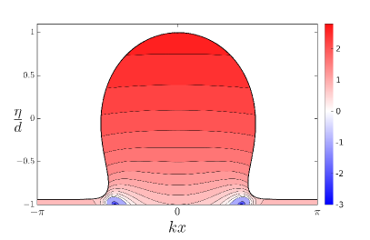
(c)

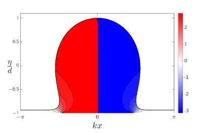
(d)

Figure 3. Iso-values of (a): $u/\sqrt{gd}$, (b): $v/\sqrt{gd}$, (c): $\log{(|w|/\sqrt{gd})}$ and (d): $\arg{(w/\sqrt{gd})}$ for the configuration displayed in figure (2).

6.2. Periodic overhanging wave

The first case of interest, as shown in figure 2, depicts a periodic overturning wave of large amplitude. This particular scenario poses significant computational challenges, making it an ideal benchmark for evaluating the robustness of our recovery procedure. Utilizing the pressure data highlighted in figure 2a, we successfully reconstruct the surface profile using the expression 5.2, resulting in excellent agreement, as evident from figure 2b. Notably, the change of variables achieved through equation 50 effectively concentrates the points in regions where $\theta_{s}$ varies the most. Consequently, we attain a high level of accuracy, with $||\eta-\eta^{\textrm{ex}}||_{\infty}\approx 4.48\times 10^{-3}$, where $\eta^{\textrm{ex}}$ corresponds to a numerical solution obtained by solving equation (36). Furthermore, for the computation of the unknown Bernoulli constant at the surface, the error is approximately $|{B}_{\mathrm{s}}-{B}_{\mathrm{s}}^{\textrm{ex}}|\approx 5.83\times 10^{-3}$.

We emphasize the effectiveness of our recovery procedure by presenting the velocity field within the fluid layer in both upper panels of figure 3. Notably, a pair of stagnation points is observed in the panel 3c on the flat bottom boundary, which often poses challenges when utilizing conformal mapping techniques. In the present context, since our methodology operates solely in the physical plane, our general approach can readily reconstruct the surface profile regardless of the presence or absence of stagnation points.

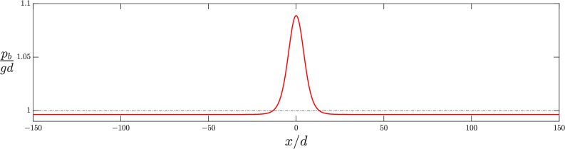
(a)

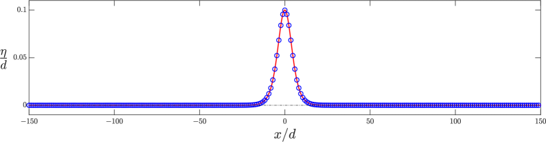
(b)

Figure 4. Surface recovery procedure for a solitary steady wave with a constant vorticity $\omega\sqrt{d/g}=1$. Both panels have the same legend than figure 2.

6.3. Rotational solitary surface wave

Computing solitary waves using our procedure is straightforward but necessitates considering a relatively large numerical domain to accurately capture their behavior far from the crest. Meanwhile, to ensure that the wave is located above the mean water level, we substitute the condition (1) with

$$\eta^{(n+1)}=\eta^{(n)}-\min\eta^{(n)},$$ (51)

instead, at each numerical iteration $n$.

The recovery process for a solitary wave is presented in figure 4, which illustrates the pressure data in the upper panel and the corresponding surface profile in the lower panel. We consider here a solitary wave of relatively small amplitude because it is quite challenging. Indeed, the larger the solitary wave, the faster its decay (thus requiring a smaller computational box) and the larger the ratio signal/noise (for field data). So, in that respect, the recovery of small amplitude solitary waves is more challenging.

In the present specific case, the agreement with a given numerical solution is great, yielding numerical errors of $||\eta-\eta^{\textrm{ex}}||_{\infty}\approx 1.46\times 10^{-4}$ and $|{B}_{\mathrm{s}}-{B}_{\mathrm{s}}^{\textrm{ex}}|\approx 4.21\times 10^{-5}$ for the surface profile and the Bernoulli constant, respectively. Unfortunately, spurious infinitesimal oscillations (located) far from the wave crest) prevent us to reach a much better accuracy that we would expect from our method. In order to facilitate these computations and remove unwanted oscillations, another change of variables can be implemented (similar to the approach (50) used for the periodic case) to concentrate the quadrature points near the crest, rather than far away where the elevation is infinitesimal. However, we reserve this task for future investigations, which will provide more comprehensive details on the efficient computation of solitary waves within this context.

7. Discussion

This work presents a novel and comprehensive boundary integral method for recovering surface water-waves from bottom pressure measurements. Despite the inherent complexity of this inverse problem, we successfully formulate the relatively simple expression (5.2) for surface recovery, enabling the computation of a wide range of rotational steady waves. A significant advantage of this approach lies in the integral formulation, which eliminates the need for arbitrarily selecting a basis of functions to fit the pressure data, as done previously in [3, 5, 7].

To demonstrate the robustness and efficiency of our method, we showcased two challenging examples: an overturning wave with a large amplitude and a solitary wave. In both cases, we accurately recovered the surface profile and the hydrodynamic parameters with good agreement. Although it might be possible to adapt our numerical procedure to compute extreme waves (with angular surface) with (or without) overhanging profiles, this task is left for future investigations. In fact, our main goal here is a proof of concept and to provide clear evidence on the effectiveness of this new formulation.

In conclusion, this article, along with the proposed boundary integral formulation, represents a significant milestone in solving the surface wave recovery problem, providing a solid foundation for future extensions, such as its potential application to three-dimensional configurations. Indeed, in 3D holomorphic functions cannot be employed but integral representations via Green functions remain, so an efficient fully nonlinear surface recovery is conceivable.

Funding. Joris Labarbe has been supported by the French government, through the $\mbox{UCA}^{\mbox{\tiny JEDI}}$ Investments in the Future project managed by the National Research Agency (ANR) with the reference number ANR-15-IDEX-01.

Declaration of interests. The authors report no conflict of interest.

Appendix A Logarithms and Polylogarithms

The function $\ln(x)$ denotes the natural logarithm (Napierian logarithm) of a real positive variable $x$ ($x\in\mathds{R}^{+}$), and $\log(z)$ denotes the principal logarithm of a complex variable $z\in\mathds{C}$, i.e.,

$$\log(z)\stackrel{{\scriptstyle\text{\tiny{def}}}}{{=}}\ln|z|+\mathrm{i}\arg(z),\qquad-\pi<\arg(z)\leqslant\pi.$$ (52)

This definition requires that the argument of any complex number lies in $]-\pi;\pi]$. It implies, in particular, that $\arg(z^{-1})=-\arg(z)$ if $z\not\in\mathds{R}^{-}$ and that $\arg(z^{-1})=\arg(z)=\pi$ if $z\in\mathds{R}^{-}$. We have the special relations

$$\log(-z) =\mathrm{i}\pi+\log(z)+2\mathrm{i}\pi\left\lfloor-\arg(z)/2\pi\right\rfloor,$$ (53)

$$\log\!\left(\mathrm{e}^{\mathrm{i}\/z}\right) =\mathrm{i}z+2\mathrm{i}\pi\left\lfloor{\textstyle{\frac{1}{2}}}-\operatorname{Re}(z/2\pi)\right\rfloor,$$ (54)

$$\log\!\left(-\mathrm{e}^{\mathrm{i}\/z}\right) =\mathrm{i}(\pi+z)+2\mathrm{i}\pi\left\lfloor-\operatorname{Re}(z/2\pi)\right\rfloor,$$ (55)

where $\left\lfloor\cdot\right\rfloor$ is the rounding toward $-\infty$.

The polylogarithms can be defined, for $|z|<1$ and $\nu\in\mathds{C}$, by

$$\mbox{\,L{\scriptsize{i}}}_{\nu}(z) =\sum_{n=1}^{\infty}{\frac{z^{n}}{n^{\nu}}},$$ (56)

and for all complex $z$ by analytic continuation [19]. With the above definition of the complex logarithm, we have the special inversion formulae

$$\mbox{\,L{\scriptsize{i}}}_{0}(z)+\mbox{\,L{\scriptsize{i}}}_{0}(z^{-1})+1 =0,$$ (57)

$$\mbox{\,L{\scriptsize{i}}}_{1}(z)-\mbox{\,L{\scriptsize{i}}}_{1}(z^{-1})+\log(-z) =\left\{\begin{array}[]{lrl}0&&\text{if}\quad z\not\in[0;1],\\ 2\/\mathrm{i}\/\pi&&\text{if}\quad z\in[0;1],\end{array}\right.$$ (60)

$$\mbox{\,L{\scriptsize{i}}}_{2}(z)+\mbox{\,L{\scriptsize{i}}}_{2}(z^{-1})+\frac{1}{2}\log^{2}(-z)+\frac{1}{6}\pi^{2} =\left\{\begin{array}[]{lrl}0&&\text{if}\quad z\not\in[0;1],\\ 2\/\mathrm{i}\/\pi\log(z)&&\text{if}\quad z\in[0;1],\end{array}\right.$$ (63)

The polylogarithms for $\nu\in\mathds{N}^{*}$ are single-valued functions in the cut plane $z\in\mathds{C}\backslash[1;+\infty[$ and the inversion formula can be used to extend their definition for $z\in[1;+\infty[$. Note that the inversion formula depends on the definition of the principal logarithm that is not unique, thus several variants can be found in the literature.

We finally note other relations useful in this paper

$$\mbox{\,L{\scriptsize{i}}}_{\nu}\!\left(\mathrm{e}^{\pm\/\mathrm{i}\/z}\right) =\mp\mathrm{i}\mathrm{d}\mbox{\,L{\scriptsize{i}}}_{\nu+1}\!\left(\mathrm{e}^{\pm\/\mathrm{i}\/z}\right)/\mathrm{d}\/z,$$ (64)

$$\mbox{\,L{\scriptsize{i}}}_{0}\!\left(\mathrm{e}^{\pm\/\mathrm{i}\/z}\right) =\pm\/{\textstyle{\frac{\mathrm{i}}{2}}}\/\cot\!\left(z/2\right)-{\textstyle{\frac{1}{2}}},$$ (65)

$$\mbox{\,L{\scriptsize{i}}}_{1}\!\left(\mathrm{e}^{\pm\mathrm{i}z}\right) =\pm\/\mathrm{i}\pi\left[\operatorname{Re}\{z\}/2\pi\right]+{\textstyle{\frac{\mathrm{i}}{2}}}\arg(z^{2})-\mathrm{i}\arg(\mp\mathrm{i}z)-{\textstyle{\frac{1}{2}}}\/\log\!\left(4\sin^{2}(z/2)\right)\mp{\textstyle{\frac{\mathrm{i}}{2}}}z$$ (66)

$$\mbox{\,L{\scriptsize{i}}}_{2}\!\left(\mathrm{e}^{\pm\/\mathrm{i}\/z}\right) =\frac{\pi^{2}}{6}+\frac{z^{2}}{4}\mp\left(\arg(z^{2})-2\arg(\mp\mathrm{i}z)\right)\frac{z}{2}\mp\frac{\mathrm{i}}{2}\int_{0}^{z}\log\!\left(4\sin^{2}\!\left(\frac{z^{\prime}}{2}\right)\right)\/\mathrm{d}\/z^{\prime},$$ (67)

where $[\cdot]$ denotes the rounding toward zero, the last relation being valid for $-2\pi<\mathrm{Re}\{z\}<2\pi$.

Appendix B Singular Leibniz integral rule

Let be $K(x,y)$ a function regular everywhere for $y\in\interval{a}{b}$, except perhaps at $y=y_{0}\in\interval[open]{a}{b}$ ($y_{0}$ generally depending on $x$, as well as $a$ and $b$) where $K$ may be singular, its finite integral being taken in the sense of Cauchy principal value, i.e.

$$J(x)=\mathchoice{{\vbox{\hbox{$\textstyle-$}}\kern-4.86108pt}}{{\vbox{\hbox{$\scriptstyle-$}}\kern-3.25pt}}{{\vbox{\hbox{$\scriptscriptstyle-$}}\kern-2.29166pt}}{{\vbox{\hbox{$\scriptscriptstyle-$}}\kern-1.875pt}}\!\int_{a(x)}^{b(x)}K(x,y)\mathrm{d}y\stackrel{{\scriptstyle\text{\tiny{def}}}}{{=}}\lim_{\epsilon\to 0^{+}}\left\{\int_{a(x)}^{y_{0}(x)-\epsilon}K(x,y)\mathrm{d}y+\int_{y_{0}(x)+\epsilon}^{b(x)}K(x,y)\mathrm{d}y\right\},$$ (68)

exists. The first derivative of $J$ is thus

$$\frac{\mathrm{d}J}{\mathrm{d}x} =\lim_{\epsilon\to 0^{+}}\left\{\frac{\mathrm{d}}{\mathrm{d}x}\int_{a}^{y_{0}-\epsilon}K(x,y)\mathrm{d}y+\frac{\mathrm{d}}{\mathrm{d}x}\int_{y_{0}+\epsilon}^{b}K(x,y)\mathrm{d}y\right\}$$

$$=\lim_{\epsilon\to 0^{+}}\left\{\int_{a}^{y_{0}-\epsilon}\frac{\partial K(x,y)}{\partial x}\mathrm{d}y+\frac{\mathrm{d}y_{0}}{\mathrm{d}x}K(x,y_{0}-\epsilon)-\frac{\mathrm{d}a}{\mathrm{d}\/x}K(x,a)\right.$$

$$\qquad\qquad\left.+\int_{y_{0}+\epsilon}^{b}\frac{\partial K(x,y)}{\partial x}\mathrm{d}y+\frac{\mathrm{d}b}{\mathrm{d}x}K(x,b)-\frac{\mathrm{d}y_{0}}{\mathrm{d}x}K(x,y_{0}+\epsilon)\right\}$$

$$=\mathchoice{{\vbox{\hbox{$\textstyle-$}}\kern-4.86108pt}}{{\vbox{\hbox{$\scriptstyle-$}}\kern-3.25pt}}{{\vbox{\hbox{$\scriptscriptstyle-$}}\kern-2.29166pt}}{{\vbox{\hbox{$\scriptscriptstyle-$}}\kern-1.875pt}}\!\int_{a}^{b}\frac{\partial K(x,y)}{\partial x}\mathrm{d}y+\frac{\mathrm{d}b}{\mathrm{d}x}K(x,b)-\frac{\mathrm{d}a}{\mathrm{d}x}K(x,a)$$

$$\quad-\frac{\mathrm{d}y_{0}}{\mathrm{d}x}\lim_{\epsilon\to 0^{+}}\left\{K(x,y_{0}+\epsilon)-K(x,y_{0}-\epsilon)\right\}.$$ (69)

For instance, $a$ and $b$ being constant and for a sufficiently well-behaving function $\varphi$, we have

$$\mathchoice{{\vbox{\hbox{$\textstyle-$}}\kern-4.86108pt}}{{\vbox{\hbox{$\scriptstyle-$}}\kern-3.25pt}}{{\vbox{\hbox{$\scriptscriptstyle-$}}\kern-2.29166pt}}{{\vbox{\hbox{$\scriptscriptstyle-$}}\kern-1.875pt}}\!\int_{a}^{b}\frac{\varphi(y)}{x-y}\mathrm{d}\/y =\mathchoice{{\vbox{\hbox{$\textstyle-$}}\kern-4.86108pt}}{{\vbox{\hbox{$\scriptstyle-$}}\kern-3.25pt}}{{\vbox{\hbox{$\scriptscriptstyle-$}}\kern-2.29166pt}}{{\vbox{\hbox{$\scriptscriptstyle-$}}\kern-1.875pt}}\!\int_{a}^{b}\frac{\partial\ln|x-y|\varphi(y)}{\partial\/x}\mathrm{d}\/y$$

$$=\frac{\mathrm{d}}{\mathrm{d}\/x}\mathchoice{{\vbox{\hbox{$\textstyle-$}}\kern-4.86108pt}}{{\vbox{\hbox{$\scriptstyle-$}}\kern-3.25pt}}{{\vbox{\hbox{$\scriptscriptstyle-$}}\kern-2.29166pt}}{{\vbox{\hbox{$\scriptscriptstyle-$}}\kern-1.875pt}}\!\int_{a}^{b}\ln|x-y|\varphi(y)\mathrm{d}\/y+\lim_{\epsilon\to 0^{+}}\ln(\epsilon)\left[\varphi(x+\epsilon)-\varphi(x-\epsilon)\right],$$ (70)

where the limit is zero if $\varphi$ is Hölder continuous (sufficient but unnecessary condition). This formula is a consequence of (B) but also of the choice of the antiderivative of $1/(x-y)$. Indeed, one can also write

$$\mathchoice{{\vbox{\hbox{$\textstyle-$}}\kern-4.86108pt}}{{\vbox{\hbox{$\scriptstyle-$}}\kern-3.25pt}}{{\vbox{\hbox{$\scriptscriptstyle-$}}\kern-2.29166pt}}{{\vbox{\hbox{$\scriptscriptstyle-$}}\kern-1.875pt}}\!\int_{a}^{b}\frac{\varphi(y)}{x-y}\mathrm{d}\/y =\mathchoice{{\vbox{\hbox{$\textstyle-$}}\kern-4.86108pt}}{{\vbox{\hbox{$\scriptstyle-$}}\kern-3.25pt}}{{\vbox{\hbox{$\scriptscriptstyle-$}}\kern-2.29166pt}}{{\vbox{\hbox{$\scriptscriptstyle-$}}\kern-1.875pt}}\!\int_{a}^{b}\frac{\partial\log(x-y)\varphi(y)}{\partial\/x}\mathrm{d}\/y$$

$$=\frac{\mathrm{d}}{\mathrm{d}\/x}\mathchoice{{\vbox{\hbox{$\textstyle-$}}\kern-4.86108pt}}{{\vbox{\hbox{$\scriptstyle-$}}\kern-3.25pt}}{{\vbox{\hbox{$\scriptscriptstyle-$}}\kern-2.29166pt}}{{\vbox{\hbox{$\scriptscriptstyle-$}}\kern-1.875pt}}\!\int_{a}^{b}\log(x-y)\varphi(y)\mathrm{d}\/y+\mathrm{i}\pi\varphi(x)+\lim_{\epsilon\to 0^{+}}\ln(\epsilon)\left[\varphi(x+\epsilon)-\varphi(x-\epsilon)\right],$$ (71)

where we have used the relations $\log(\epsilon)=\ln(\epsilon)$ and $\log(-\epsilon)=\ln(\epsilon)+\mathrm{i}\pi$, since $\epsilon\in\mathds{R}^{+}$. The relation (70) is more convenient when dealing only with real variables, while (71) is more suitable for complex formulations. The reason behind the latter argument is because $\log(x)$ can be continued analytically in the complex plane, which is not the case with $\ln|x|$.

References

- Bergan et al. [1969] P. Bergan, A. Tørum, and A. Traetteberg. Wave measurements by a pressure type wave gauge. Coastal Engineering 1968, pages 19–29, 1969.
- Boyd [2001] J. P. Boyd. Chebyshev and Fourier spectral methods. Courier Corporation, 2001.
- Clamond [2013] D. Clamond. New exact relations for easy recovery of steady wave profiles from bottom pressure measurements. J. Fluid Mech., 726:547–558, 2013.
- Clamond [2018] D. Clamond. New exact relations for steady irrotational two-dimensional gravity and capillary surface waves. Phil. Trans. R. Soc. A, 376(2111):20170220, 2018.
- Clamond and Constantin [2013] D. Clamond and A. Constantin. Recovery of steady periodic wave profiles from pressure measurements at the bed. J. Fluid Mech., 714:463–475, 2013.
- Clamond and Henry [2020] D. Clamond and D. Henry. Extreme water-wave profile recovery from pressure measurements at the seabed. J. Fluid Mech., 903:R3, 12, 2020.
- Clamond et al. [2023] D. Clamond, J. Labarbe, and D. Henry. Recovery of steady rotational wave profiles from pressure measurements at the bed. J. Fluid Mech., 961:R2, 2023.
- Constantin [2006] A. Constantin. The trajectories of particles in Stokes waves. Invent. Math., 3:523–535, 2006.
- Constantin [2012] A. Constantin. On the recovery of solitary wave profiles from pressure measurements. J. Fluid Mech., 699:376–384, 2012.
- Constantin and Strauss [2010] A. Constantin and W. Strauss. Pressure beneath a Stokes wave. Comm. Pure App. Math, 63:533–557, 2010.
- Da Silva and Peregrine [1988] A. T. Da Silva and D. H. Peregrine. Steep, steady surface waves on water of finite depth with constant vorticity. J. Fluid Mech., 195:281–302, 1988.
- Lee and Wang [1985] D. Lee and H. Wang. Measurement of surface waves from subsurface gage. Coastal Engineering 1984, pages 271–286, 1985.
- Lin and Yang [2020] M. Lin and C. Yang. Ocean observation technologies: A review. Chin. J. Mech. Eng., 33(1):1–18, 2020.
- Longuet-Higgins [1986] M. S. Longuet-Higgins. Eulerian and Lagrangian aspects of surface waves. J. Fluid Mech., 173:683–707, 1986.
- Oliveras et al. [2012] K. L. Oliveras, V. Vasan, B. Deconinck, and D. Henderson. Recovering the water-wave profile from pressure measurements. SIAM J. Appl. Math., 72(3):897–918, 2012.
- Patterson Jr and Orszag [1971] G. S. Patterson Jr and S. A. Orszag. Spectral calculations of isotropic turbulence: Efficient removal of aliasing interactions. Phys. Fluids, 14(11):2538–2541, 1971.
- Tsai and Tsai [2009] J. C. Tsai and C. H. Tsai. Wave measurements by pressure transducers using artificial neural network. Ocean Eng., 36(15–16):1149–1157, 2009.
- Vanden-Broeck [1994] J. M. Vanden-Broeck. Steep solitary waves in water of finite depth with constant vorticity. J. Fluid Mech., 274:339–348, 1994.
- Wood [1992] D. C. Wood. The computation of polylogarithms. Technical Report 15-92, University of Kent Computing Laboratory, Canterbury, UK, 1992.