Computational complexity of counting coincidences

Abstract.

Can you decide if there is a coincidence in the numbers counting two different combinatorial objects? For example, can you decide if two regions in $\mathbb{R}^{3}$ have the same number of domino tilings? There are two versions of the problem, with  $2\times 1\times 1$  and  $2\times 2\times 1$  boxes. We prove that in both cases the coincidence problem is not in the polynomial hierarchy unless the polynomial hierarchy collapses to a finite level. While the conclusions are the same, the proofs are notably different and generalize in different directions.

We proceed to explore the coincidence problem for counting independent sets and matchings in graphs, matroid bases, order ideals and linear extensions in posets, permutation patterns, and the Kronecker coefficients. We also make a number of conjectures for counting other combinatorial objects such as plane triangulations, contingency tables, standard Young tableaux, reduced factorizations and the Littlewood–Richardson coefficients.

1. Introduction

1.1. Tilings

In this paper we consider coincidences of combinatorial counting functions. Consider two bounded regions in the plane. Do they have the same number of domino tilings? Here we are assuming that the regions are finite subsets of unit squares on a square grid, we write  $\Gamma\subset\mathbb{Z}^{2}$, and the dominos are the usual  $2\times 1$  rectangles. For example, a  $2\times 3$  rectangle has three domino tilings, and both regions on the right have four domino tilings:

Algorithmically, the coincidence problem is easy, since we can simply compute the number of domino tilings of each region in polynomial time, and then compare the numbers. Indeed, the Kasteleyn formula  gives the number  $\tau(\Gamma)$  of domino tilings as an  $n\times n$ determinant which can be computed in time polynomial in $n$, where  $n=|\Gamma|$  is the area of region $\Gamma$, see e.g. [Ken04, LP09].

Now consider what happens to domino tilings in $\mathbb{R}^{3}$. Should we expect that the coincidence problem remains easy? It turns out, this is a much harder problem. In fact, there are two versions of $3$-dimensional dominoes: a  $2\times 2\times 1$  box which we call a slab, and a  $2\times 1\times 1$  box which we call a brick. For example, there are three tilings of a  $2\times 2\times 2$  box with a slab and nine with a brick, shown below up to rotations:

For both versions, there is no analogue of the Kasteleyn formula for the number of tilings. Indeed, for tilings with slabs or with bricks, Jed Yang and the second author proved that computing the number of tilings is #P-complete [PY13a]. But this is where the similarities end: the coincidence problems have very different nature in these two cases. The reason for the difference is the type of reduction used in the proofs (see Section 4 and $\S$6.2).

Let  $\tau_{s}(\Gamma)$  be the number of tilings of a region  $\Gamma\subset\mathbb{Z}^{3}$  with slabs. Denote by  C${}_{\text{ST}}$  the slab tiling coincidence problem:

(1.1) $$\text{\sc C${}_{\text{ST}}$}\ :=\ \big{\{}\hskip 1.70709pt\tau_{s}(\Gamma)\hskip 0.85355pt=^{?}\hskip 0.85355pt\tau_{s}(\Gamma^{\prime}),\ \ \text{where}\ \ \Gamma,\Gamma^{\prime}\subset\mathbb{Z}^{3}\big{\}}.$$

Theorem 1.1.

Problem  C${}_{\text{ST}}$  is  coNP-hard. Furthermore,  C${}_{\text{ST}}$  is not in the polynomial hierarchy unless the polynomial hierarchy collapses to a finite level:   C${}_{\text{ST}}$  $\in\textup{{{PH}}}\ \Rightarrow\ \textup{{{PH}}}=\Sigma^{{\textup{p}}}_{m}$  for some $m$.

In particular, the theorem implies that  C${}_{\text{ST}}$  does not have a polynomial time algorithm (unless $\textup{{{P}}}=\textup{{{NP}}}$). Nor does it have a probabilistic polynomial time algorithm (unless PH collapses), since  $\textup{{{BPP}}}\subseteq\textup{{{PH}}}$. Nor does there exist a polynomial size witness for the coincidence (ditto).

The first part of the theorem follows immediately from NP-completeness of the slab tileability [PY13a, Thm 1.1], which is a special cases of the  C${}_{\text{ST}}$. The second part follows from the parsimonious reduction in the proof of #P-completeness of the  C${}_{\text{ST}}$, combined with some known computational complexity (see $\S$4.1).

Let  $\tau_{b}(\Gamma)$  be the number of tilings of a region  $\Gamma\subset\mathbb{Z}^{3}$  with bricks. We similarly denote by  C${}_{\text{BT}}$  the brick tiling coincidence problem:

(1.2) $$\text{\sc C${}_{\text{BT}}$}\ :=\ \big{\{}\hskip 1.70709pt\tau_{b}(\Gamma)\hskip 0.85355pt=^{?}\hskip 0.85355pt\tau_{b}(\Gamma^{\prime}),\ \ \text{where}\ \ \Gamma,\Gamma^{\prime}\subset\mathbb{Z}^{3}\big{\}}.$$

Theorem 1.2.

Problem  C${}_{\text{BT}}$  is not in the polynomial hierarchy unless the polynomial hierarchy collapses to a finite level:   C${}_{\text{BT}}$  $\in\textup{{{PH}}}\ \Rightarrow\ \textup{{{PH}}}=\Sigma^{{\textup{p}}}_{m}$  for some $m$.

Note that we make no claims that  C${}_{\text{BT}}$  is  coNP-hard. Proof of that would require a major advance in computational complexity. However, the theorem does imply that  C${}_{\text{BT}}$  is not in  P,  BPP,  NP,  coNP, etc., unless  $\textup{{{PH}}}=\Sigma^{{\textup{p}}}_{m}$. For the proof we again need some standard results in computational complexity, combined with a curious combinatorial result of independent interest (Theorem 3.1).

1.2. Beyond tilings

The paper starts with proofs of two theorems above which allows us to develop tools to prove similar results for the coincidence problem of many other combinatorial counting functions. We group the results into two, by analogy with the two theorems above.

Let  $f\in\textup{{{\#P}}}$  be a counting function. The coincidence problem  C_f  is defined as follows:

$$\text{\sc C}_{f}\ :=\ \big{\{}\hskip 0.85355ptf(x)\hskip 1.70709pt=^{?}\hskip 0.85355ptf(y)\hskip 0.85355pt\big{\}}.$$

Theorem 1.3.

The coincidence problem  C_f  is not in the polynomial hierarchy unless the polynomial hierarchy collapses to a finite level, where  $f$  is either one of the following:

$(0)$  the number of satisfying assignments of a  3SAT  formula,

$(1)$  the number of proper $3$-colorings of a planar graph,

$(2)$  the number of Hamiltonian cycles in a graph,

$(3)$  the number  $\mathrm{PC}_{\pi}(\sigma)$  of patterns $\hskip 0.85355pt\pi\hskip 0.85355pt$ in a permutation $\hskip 0.85355pt\sigma$,

$(4)$  the Kronecker coefficient  $g(\lambda,\mu,\nu)$  for partitions  $\lambda,\mu,\nu\vdash n$  given in unary.

Furthermore, the coincidence problem  C_f  is  coNP-hard in all these cases.

As we explain, the theorem follows from known complexity results. This is in sharp contrast with our next theorem where each part requires additional work. We need just one definition.

A rational matroid  is a matroid that is realizable over $\mathbb{Q}$. We assume that this matroid is given by a set of $n$ vectors in $\mathbb{Q}^{d}$. In this presentation, computing the number  $b(M)$  of bases of a rational matroid $M$ is known to be #P-complete [Sno12] (cf. $\S$6.3).

Theorem 1.4 (main theorem).

The coincidence problem  C_f  is not in the polynomial hierarchy unless the polynomial hierarchy collapses to a finite level, where  $f$  is either of the following:

$(0)$  the number of perfect matchings  $\mathrm{PM}(P)$  in a simple bipartite graph,

$(1)$  the number of satisfying assignments of a  MONOTONE 2SAT  formula,

$(2)$  the number of independent sets  $\lambda(G)$  in a planar bipartite graph,

$(3)$  the number of order ideals  $\mu(P)$  of a poset,

$(4)$  the number of linear extensions  $e(P)$  of a $2$-dimensional poset,

$(5)$  the number of matchings  ${\rm ma}(G)$  in a planar bipartite graph,

$(6)$  the number of bases  $b(M)$  of a rational matroid.

Note that all counting functions in Theorems 1.3 and 1.4 are  #P-complete. Unfortunately, that by itself does not imply that the corresponding coincidence problems are not in PH (see $\S$6.18). Example 5.15 (see also $\S$6.4) has an especially notable variation on part $(4)$ in the theorem for posets of height two. While the number of linear extensions is known to be  #P-complete in this case, it is open whether the corresponding coincidence problem is in PH. Similarly, a variation on part $(6)$ for bicircular matroids gives another example of this type (see $\S$6.3). The number of bases is known to be  #P-complete in this case, but corresponding coincidence problem remains unexplored.

Paper structure

We start with basic definitions and notation in a short Section 2. In Section 3, we give some preliminary results on domino tilings. In Section 4, we prove Theorems 1.1, 1.2 and 1.3. In a lengthy Section 5, we discuss further examples, and prove Main Theorem 1.4. We conclude with many final remarks and open problems in Section 6.

2. Definitions and notation

General notation

Let  $[n]=\{1,\ldots,n\}$  and  $\mathbb{N}=\{0,1,2,\ldots\}$. For a sequence  $\textbf{{a}}=(a_{1},\ldots,a_{m})$, denote  $|a|:=a_{1}+\ldots+a_{m}$ . Similarly, for the integer partitions  $\mu\subset\lambda$, let the size  $|\lambda/\mu|$  be the number of squares in the skew Young diagram $\lambda/\mu$. For  $|\lambda|=n$  we also write  $\lambda\vdash n$.

Combinatorics

We think of  $\mathbb{Z}^{d}\subset\mathbb{R}^{d}$  both as a lattice and a collection of the corresponding unit $d$-cube. A region  $\Gamma\subset\mathbb{Z}^{d}$  is a subset of $d$-cubes. Denote by  $|\Gamma|$  the size of $\Gamma$, which can also be viewed as the volume of the union of the corresponding unit cubes. Region  $\Gamma$  is called simply connected if the union of the corresponding (closed) $d$-cubes is simply connected. A tile  in  $\mathbb{R}^{d}$  is a finite simply connected region. For a set of tiles  $T=\{t_{1},\ldots,t_{m}\}$, a tiling  is a disjoint union of copies of tiles $t_{i}$ (unless stated otherwise, parallel translations, rotations and reflections are allowed).

We assume that the reader is familiar with basic notions in algebraic combinatorics, such as  standard Young tableaux, Kostka numbers, Littlewood–Richardson  and Kronecker coefficients. Defining them, explaining their importance, combinatorial interpretations and properties would take too much space and be a distraction. We refer the reader to [Mac95, Man01, Sta12] and further references sprinkled throughout the paper.

Complexity

We assume that the reader is familiar with basic notions and results in computational complexity and only recall a few definitions. We use standard complexity classes  P,  NP, coNP,  #P,  $\Sigma^{{\textup{p}}}_{m}$  and  PH. The notation  $\{a=^{?}b\}$  is used to denote the decision problem whether  $a=b$. We use the oracle notation  K${}^{\text{\sf L}}$  for two complexity classes  K, L $\subseteq\textup{{{PSPACE}}}$, and the polynomial closure  $\langle$A$\rangle$ for a problem  A $\in\textup{{{PSPACE}}}$. We will also use less common classes

$$\textup{{{GapP}}}:=\{f-g\mid f,g\in\textup{{{\#P}}}\}\quad\text{and}\quad{\textup{{{C${}_{=}$P}}}}:=\{f(x)=^{?}g(y)\mid f,g\in\textup{{{\#P}}}\}.$$

The distinction between binary  and unary  presentation will also be important. We refer to [GJ78] and [GJ79, $\S$4.2] for the corresponding notions of NP-completeness and strong  NP-completeness.

We also that assume the reader is familiar with standard decision and counting problems, such as  2SAT,  MONOTONE 2SAT,  3SAT,  1-in-3 SAT,  HAMILTON CYCLE,  #2SAT,  #3SAT,  PERMANENT, etc. Occasionally, we conflate counting functions $f$ and the problems of computing $f$. We hope this does not lead to a confusion.

We refer to [AB09, Gol08, MM11, Pap94] for definitions and standard results in computational complexity. See [GJ79] for the classical introduction and a long list of NP-complete problems. See also [Pak22, $\S$13] for a recent overview of #P-complete problems in combinatorics. For surveys on counting complexity, see [For97, Sch90].

3. Counting tilings

3.1. Domino tilings

Denote by  $\mathcal{T}(n)$  the set of numbers of domino tilings over all regions of size $2n$:

$$\mathcal{T}(n)\ :=\ \big{\{}\hskip 1.70709pt\tau(\Gamma)\hskip 1.70709pt,\ \ \text{where}\ \ \Gamma\subset\mathbb{Z}^{2},\ |\Gamma|\hskip 0.85355pt=\hskip 0.85355pt2n\hskip 1.70709pt\big{\}}.$$

Clearly,  $\mathcal{T}(n)\subseteq\{0,1,\ldots,4^{n}\}$  since each domino tilings is determined by the $4$ choices for a domino at every even square. The following result proves a converse:

Theorem 3.1.

There is a constant  $c>1$, such that  $\mathcal{T}(n)\supseteq\{0,1,\ldots,c^{n}\}$, for all  $n\geq 1$. Moreover, for all  $k\leq c^{n}$, a region  $\Gamma\subset\mathbb{Z}^{2}$  with  $\tau(\Gamma)=k$  and  $|\Gamma|=2n$, can be constructed in time polynomial in $n$.

Remark 3.2.

It was known before that  $\cup_{n}\mathcal{T}(n)=\mathbb{N}$, i.e. that every nonnegative integer is the number of domino tilings of some  region. This was shown by Philippe Nadeau with an elegant explicit construction. Unfortunately, this construction has  $\tau(\Gamma)=\Theta(n)$  where  $n=|\Gamma|$, and thus does not give our theorem.

In a different direction, Brualdi and Newman in [BN65] gave (in the language of permanents), an explicit construction of a simple bipartite graph on  $n$  vertices with exactly $k$ perfect matchings, for all  $0\leq k\leq 2^{n-1}$. These graphs have unbounded degree and thus very far from being grid graphs (or even planar graphs). There was a recent constant factor improvement in [GT18], but relatively little attention otherwise (see [OEIS, A089477]), compared to the corresponding determinant problem (see $\S$6.10).

Proof of Theorem 3.1.

For an integer  $k\geq 0$, we give an explicit construction of a region  $\Gamma\subset\mathbb{Z}^{2}$  with  $\tau(G)=k$  and  $|\Gamma|=O(\log k)$. This implies the result.

A square  $(i,j)\in\mathbb{Z}^{2}$  is called even (odd ) if  $i+j$  is even (odd). Denote by  $\Gamma_{e}=\Gamma\cap\mathbb{Z}_{e}^{2}$  and  $\Gamma_{o}:=\Gamma\cap\mathbb{Z}_{o}^{2}$  the sets of even and odd squares in $\Gamma$, respectively. Clearly, if  $|\Gamma_{e}|\neq|\Gamma_{o}|$  then  $\tau(\Gamma)=0$. We use  $\Gamma-x-y$  to denote $\Gamma$ with squares $x,y$ removed. Denote by  $\mathcal{D}(a,b)$  the set of regions  $\Gamma$ such that  $\tau(\Gamma)=a$  and  $\tau(\Gamma-x-y)=b$  for some  $x\in\Gamma_{e}$  and  $y\in\Gamma_{o}$.

Below we give constructions which prove the following implications:

(3.1) $$\mathcal{D}(a,1)\neq\varnothing\ \Longrightarrow\ \mathcal{D}(2a,1)\neq\varnothing\hskip 0.85355pt,$$

$$\mathcal{D}(a,1)\neq\varnothing\ \Longrightarrow\ \mathcal{D}(2a+1,1)\neq\varnothing\hskip 0.85355pt.$$

Starting with  $\mathcal{D}(1,1)\neq\varnothing$  and iterating these in  $O(\log k)$  times gives the desired  $\Gamma\in\mathcal{D}(k,1)$.

For a region  $\Gamma$  and squares  $x,y\in\Gamma$, we say that  $(\Gamma,x,y)$  is a $C$-triple  if

$\circ$   $x=(i,j)\in\Gamma_{e}$  and  $y=(i,j+7)\in\Gamma_{o}$ ,

$\circ$   $(u,v)\notin\Gamma$  for all  $u>i$,

$\circ$   $(u,v)\notin\Gamma$  for all  $i-1\leq u\leq i$  and  $j+1\leq v\leq j+6$.

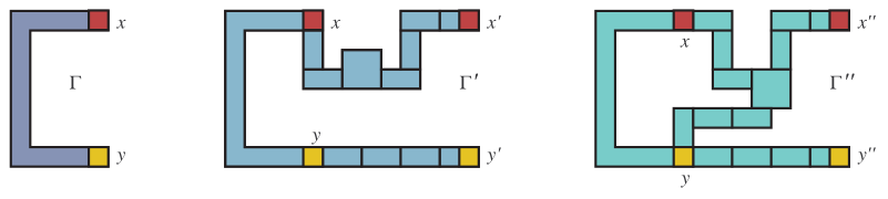
Figure 3.1. Region $\Gamma\in\mathcal{D}(1,1)$, and two transformations  $\Gamma\in\mathcal{D}(a,1)\hskip 0.85355pt\Rightarrow\hskip 0.85355pt\Gamma^{\prime}\in\mathcal{D}(2a,1)$, and  $\Gamma\in\mathcal{D}(a,1)\hskip 0.85355pt\Rightarrow\hskip 0.85355pt\Gamma^{\prime\prime}\in\mathcal{D}(2a+1,1)$.

We start with a $C$-triple  $(\Gamma,x,y)\in\mathcal{D}(1,1)$  as in Figure 3.1. We then define two transformations  $(\Gamma,x,y)\to(\Gamma^{\prime},x^{\prime},y^{\prime})$  and  $(\Gamma,x,y)\to(\Gamma^{\prime\prime},x^{\prime\prime},y^{\prime\prime})$  as in the figure, which prove the implications (3.1). Note that in both cases we obtain two $C$-triples by adding at most 30 squares. This completes the construction. ∎

Corollary 3.3.

In notation of the proof above, we have  $\mathcal{D}(a,b)\neq\varnothing$  for all  $a,b\geq 0$.

Proof.

By modifying our two transformations, one can show that

(3.2) $$\mathcal{D}(a,b)\neq\varnothing\ \Longrightarrow\ \mathcal{D}(b,a)\neq\varnothing\hskip 0.85355pt,$$

$$\mathcal{D}(a,b)\neq\varnothing\hskip 0.85355pt,\ \mathcal{D}(a^{\prime},b^{\prime})\neq\varnothing\ \Longrightarrow\ \mathcal{D}(aa^{\prime}+bb^{\prime},bb^{\prime})\neq\varnothing\hskip 0.85355pt.$$

The first of these is given by  $(\Gamma,x,y)\to(\Gamma^{\prime},x^{\prime},y^{\prime})$  as in Figure 3.2. Similarly, the second is given by $(\Gamma,x,y),(\Gamma,x^{\prime},y^{\prime})\to(\Gamma^{\prime\prime},x,y^{\prime})$  as in the figure. Note that  $(\Gamma^{\prime\prime},x,y^{\prime})$  is no longer a $C$-triple, so this transformation can be used only once.

In the proof above, we showed that  $\mathcal{D}(n,1)\neq\varnothing$  for all  $n\geq 0$. By the first transformation in (3.2), this implies that  $\mathcal{D}(1,m)\neq\varnothing$  for all  $m\geq 0$. Therefore, by the second transformation in (3.2), we have  $\mathcal{D}(m+n,m)\neq\varnothing$. We then have  $\mathcal{D}(m,m+n)\neq\varnothing$  by the first (after a modification where $x^{\prime}$ and $y^{\prime}$ are above and placed below $x^{\prime}$ and $y^{\prime}$, respectively). Note that the second transformation is used only here, and thus the construction is well defined.

The remaining cases in  $\mathcal{D}(n,0)$  and  $\mathcal{D}(0,n)$, follow from the two transformations above applied to  $\mathcal{D}(1,0)$. Alternatively, they follow the last two transformations in Figure 3.2; the details are straightforward. This finishes the proof. ∎

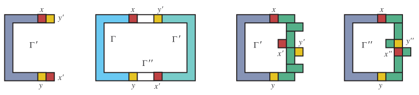
Figure 3.2. Four transformations:  $\Gamma\in\mathcal{D}(a,b)\hskip 0.85355pt\Rightarrow\hskip 0.85355pt\Gamma^{\prime}\in\mathcal{D}(b,a)$,   $\Gamma\in\mathcal{D}(a,b)$,  $\Gamma^{\prime}\in\mathcal{D}(a^{\prime},b^{\prime})\hskip 0.85355pt\Rightarrow\hskip 0.85355pt\Gamma^{\prime\prime}\in\mathcal{D}(aa^{\prime}+bb^{\prime},bb^{\prime})$,  $\Gamma\in\mathcal{D}(a,b)\hskip 0.85355pt\Rightarrow\hskip 0.85355pt\Gamma^{\prime}\in\mathcal{D}(0,a)$   and   $\Gamma\in\mathcal{D}(a,b)\hskip 0.85355pt\Rightarrow\hskip 0.85355pt\Gamma^{\prime\prime}\in\mathcal{D}(a,0)$.

Corollary 3.4.

Let  $\mathcal{D}^{\prime}(a,b)$  be the set of regions  $\Gamma$ such that  $\tau(\Gamma)=a$  and  $\tau(\Gamma-x-y)=b$  for some domino  $(x,y)$, where  $x,y\in\Gamma$. Then  $\mathcal{D}^{\prime}(a,b)\neq\varnothing$,  for all  $0\leq b\leq a$.

Proof.

Note that if  $(x,y)$  is a domino in $\Gamma$, then  $\tau(\Gamma-x-y)\leq\tau(\Gamma)$. Thus the assumption  $b\leq a$  in the claim. Now, for  $\Gamma\in\mathcal{D}(a-b,1)$  where  $b\geq 1$, and  $\Gamma^{\prime}\in\mathcal{D}(1,b)$, the second transformation in (3.2) gives a region  $\Gamma^{\prime\prime}\in\mathcal{D}(a,b)$  as in Figure 3.2. Removing one white domino and keeping the other, gives the desired region in  $\mathcal{D}^{\prime}(a,b)$.

Similarly, taking a region  $\Gamma\subset\mathbb{Z}^{2}$  with  $\tau(\Gamma)=a$, attaching a domino $(x,y)$ to a top right square  $z\in\Gamma$  gives region  $\Gamma^{\prime}\in\mathcal{D}^{\prime}(a,0)$  since  $\tau(\Gamma+x+y)=\tau(\Gamma)$  and  $\tau(\Gamma-x-z)=0$. The details are straightforward. ∎

3.2. Slab tilings

Denote by  $\mathcal{T}_{s}(n)$  the set of numbers of tilings with slabs:

$$\mathcal{T}_{s}(n)\ :=\ \big{\{}\hskip 1.70709pt\tau_{s}(\Gamma)\hskip 1.70709pt,\ \ \text{where}\ \ \Gamma\subset\mathbb{Z}^{3},\ |\Gamma|\hskip 0.85355pt=\hskip 0.85355pt4n\hskip 1.70709pt\big{\}}.$$

Theorem 3.5.

There is a constant  $c>1$, such that  $\mathcal{T}_{s}(n)\supseteq\{0,1,\ldots,c^{n}\}$, for all  $n\geq 1$. Moreover, for all  $k\leq c^{n}$, a region  $\Gamma\subset\mathbb{Z}^{3}$  with  $\tau_{s}(\Gamma)=k$  and  $|\Gamma|=2n$, can be constructed in time polynomial in $n$.

Note that the corresponding result for the set  $\mathcal{T}_{b}(n)$  of numbers of tiling with bricks, follows trivially from Theorem 3.1 since  $\mathcal{T}(n)\subseteq\mathcal{T}_{b}(n)$.

Proof of Theorem 3.5.

The result follows from the proof of Theorem 3.1. Indeed, for every region  $\Gamma\subset\mathbb{Z}^{2}$  we can take a 2-layered region  $\Gamma_{2}:=\Gamma\times\{0,1\}\subset\mathbb{Z}^{3}$. Assuming  $\Gamma$  does not have a  $2\times 2$  square inside, we have  $\tau_{s}(\Gamma_{2})=\tau(\Gamma)$. The result now follows from reductions in Figure 3.1, where the  $2\times 2$  square in the middle is replaced by a  $3\times 3$  square without a center square (see an example below). Note that the notion of $C$-triples also needs to be adjusted accordingly. The details are straightforward. ∎

4. Complexity of coincidences

4.1. Parsimonious reductions

Let  $f\in\textup{{{\#P}}}$  be a counting function. As in the introduction, denote by

$$\text{\sc C}_{f}\ :=\ \big{\{}\hskip 0.85355ptf(x)\hskip 1.70709pt=^{?}\hskip 0.85355ptf(y)\hskip 0.85355pt\big{\}}$$

the coincidence problem  for $f$  (cf. 6.1). This problem naturally belongs to the complexity class

(4.1) $${\textup{{{C${}_{=}$P}}}}:=\big{\{}\hskip 0.85355ptf(x)\hskip 1.70709pt=^{?}\hskip 0.85355ptg(y)\ \text{where}\ f,\hskip 1.70709ptg\hskip 0.85355pt\in\hskip 0.85355pt\textup{{{\#P}}}\hskip 0.85355pt\big{\}}.$$

Note that  $\textup{{{coNP}}}\subseteq{\textup{{{C${}_{=}$P}}}}$, by definition. The  #3SAT  coincidence problem  C${}_{\text{\sc\#3SAT}}$  is a complete problem in this class.

Function  $f$  is said to have a parsimonious reduction  to $g$, if there is an injection  $\rho:x\to y$  from the instances of $f$ to the instances of $g$, which maps values of the functions:  $f(x)=g(y)$, and such that $\rho$ can be computed in polynomial time. If  #3SAT  has a parsimonious reduction to $f$, then the coincidence problem  C_f  is  coNP-hard because the decision problem  3SAT  is  NP-complete. Moreover,  C_f  is  C₌P-complete by the definition of  C₌P. In general, there are other ways for a problem to be  C₌P-complete, but having a parsimonious reduction is the most straightforward.

Proposition 4.1 (cf. Theorem 1.3, part $(0)$).

Let  $f\in\textup{{{\#P}}}$  be a function with a parsimonious reduction from  #3SAT. Then the coincidence problem  C_f  is not in  PH, unless  $\textup{{{PH}}}=\Sigma^{{\textup{p}}}_{m}$  for some $m$.

Proof.

Suppose that  C${}_{f}\in\textup{{{PH}}}$. Then  C${}_{f}\in\hskip 0.85355pt\Sigma^{{\textup{p}}}_{n}$  for some $n$. We then have:

(4.2) $$\textup{{{PH}}}\hskip 1.70709pt\subseteq\hskip 1.70709pt\textup{{{NP}}}^{{\textup{{{C${}_{=}$P}}}}}\hskip 1.70709pt\subseteq\hskip 1.70709pt\textup{{{NP}}}^{\langle\text{\sc C}_{\text{\sc\#3SAT}}\rangle}\hskip 1.70709pt\subseteq\hskip 1.70709pt\textup{{{NP}}}^{\langle\text{{\sc C}}_{f}\rangle}\hskip 1.70709pt\subseteq\hskip 1.70709pt\textup{{{NP}}}^{\Sigma^{{\textup{p}}}_{n}}\hskip 1.70709pt\subseteq\hskip 1.70709pt\Sigma^{{\textup{p}}}_{n+1}\,,$$

where the first inclusion is by Tarui [Tar91] (see also [Gre93]), the second inclusion follows since  C${}_{\text{\sc\#3SAT}}$  is a complete problem in C₌P, the third follows from the parsimonious reduction of  #3SAT  to $f$, and the last inclusion is by definition. This proves the desired collapse of the polynomial hierarchy. ∎

Proof of Theorem 1.1.

The NP-completeness of  SlabTileability  is proved in [PY13a] by a bijective reduction from  1-in-3 SAT. Since Schaefer’s reduction  of  1-in-3 SAT  from  3SAT  is also by a bijection [Sch78] (see also [GJ79, Problem LO4]), we conclude that the number of slab tilings has a parsimonious reduction from  #3SAT. The result now follows from Proposition 4.1. ∎

Proof of Theorem 1.3, parts $(1)$, $(2)$.

These follow immediately from Proposition 4.1 and parsimonious reductions from #3SAT  given in [GJ79]. ∎

4.2. Pattern containment

Let  $\pi\in S_{k}$  and  $\sigma\in S_{n}$. We say that  $\sigma$  contains  $\pi$  if there is  $A=\{a_{1}<\ldots<a_{k}\}\subset[n]$, such that  $\sigma(a_{1}),\ldots,\sigma(a_{k})$  has the same relative order as $\hskip 0.85355pt\pi$. Denote by  $\mathrm{PC}_{\pi}(\sigma)$  the number of subsets $A$ as above. This counting functions is well studied in various settings, see e.g. [Kit11, Vat15].

Define the pattern containment coincidence problem:

$$\text{\sc C}_{\text{\sc PC}}\,=\,\big{\{}\hskip 0.85355pt\mathrm{PC}_{\pi}(\sigma)\hskip 1.70709pt=^{?}\hskip 0.85355pt\mathrm{PC}_{\pi^{\prime}}(\sigma^{\prime})\hskip 0.85355pt\big{\}}.$$

Proof of Theorem 1.3, part $(3)$.

It was shown in [BBL98, Cor. 4], that computing the pattern containment function  $\mathrm{PC}_{\pi}(\sigma)$  is #P-complete, and the proof uses a parsimonious reduction from  #3SAT. Now the theorem follows from Proposition 4.1. ∎

4.3. Kronecker coefficients

Consider the following application of the tools above to algebraic combinatorics. Let  $g(\lambda,\mu,\nu)$, where $\lambda,\mu,\nu\vdash n$, denote the Kronecker coefficients:

$$g(\lambda,\mu,\nu)\,:=\,\langle\chi^{\lambda}\chi^{\mu},\chi^{\nu}\rangle\,=\,\frac{1}{n!}\hskip 1.70709pt\sum_{\sigma\in S_{n}}\hskip 1.70709pt\chi^{\lambda}(\sigma)\hskip 1.70709pt\chi^{\mu}(\sigma)\hskip 1.70709pt\chi^{\nu}(\sigma)\hskip 1.70709pt,$$

where  $\chi^{\lambda}$  denote the irreducible $S_{n}$ character corresponding to $\lambda\vdash n$. By definition,  $g(\lambda,\mu,\nu)\in\mathbb{N}$  and is symmetric with respect to permutations of  $\lambda,\mu,\nu$. It is known that  $g$  is in  $\textup{{{GapP}}}:=\textup{{{\#P}}}-\textup{{{\#P}}}$, i.e. can be written as the difference of two functions in #P. It is a major open problem whether  $g$  is in #P. Here and below we are assuming that partitions are given in unary. We refer to recent surveys [Pak22, Pan23] for further background.

Define the Kronecker coefficients coincidence problem:

$$\text{\sc C}_{\text{\sc KRON}}\,=\,\big{\{}\hskip 0.85355ptg(\lambda,\mu,\nu)\hskip 1.70709pt=^{?}\hskip 0.85355ptg(\alpha,\beta,\gamma)\hskip 0.85355pt\big{\}}.$$

Proof of Theorem 1.3, part $(4)$.

It was shown in [IMW17] that the Kronecker vanishing problem  $\{g(\lambda,\mu,\nu)=^{?}0\}$  is  coNP-hard. This proves the first part. For the second part, recall that computing  $g$  is  #P-hard (in the unary) [IMW17], and that the original proof gives an explicit (although rather involved) parsimonious reduction from  #3SAT  to $\hskip 0.85355ptg$. Now the theorem follows from Proposition 4.1. ∎

4.4. The permanent

We start with a more general problem which will be used to demonstrate our approach. Recall that the  0/1 Permanent  is the benchmark #P-complete problem, which corresponds to counting perfect matchings in simple bipartite graphs.

Let  C${}_{\text{\sc PER}}$  denote the  0/1 Permanent Coincidence problem:

$$\text{\sc C${}_{\text{\sc PER}}$}\ :=\ \big{\{}\mathrm{per}(M)\,=^{?}\,\mathrm{per}(M^{\prime})\hskip 1.70709pt\mid\hskip 1.70709ptM,\hskip 0.85355ptM^{\prime}\in\mathcal{M}_{n}\big{\}},$$

where  $\mathcal{M}_{n}$  is the set of $n\times n$  matrices with entries in $\{0,1\}$.

Theorem 4.2 (= Theorem 1.4, part $(0)$).

C${}_{\text{\sc PER}}$ $\notin\textup{{{PH}}}$  unless  $\textup{{{PH}}}=\Sigma^{{\textup{p}}}_{m}$  for some $\hskip 0.85355ptm$.

Proof.

Let  V${}_{\text{\sc PER}}$  denote the  0/1 Permanent Verification problem:

$$\text{\sc V${}_{\text{\sc PER}}$}\ :=\ \big{\{}\mathrm{per}(M)\,=^{?}\,k\big{\}},$$

where  $M$  is a 0/1 matrix and  $k\in\mathbb{N}$  is given in binary. We have:

(4.3) $$\textup{{{PH}}}\hskip 1.70709pt\subseteq\hskip 1.70709pt\textup{{{P}}}^{\textup{{{\#P}}}}\hskip 1.70709pt\subseteq\hskip 1.70709pt\textup{{{NP}}}^{\langle\text{\sc V${}_{\text{\sc PER}}$}\rangle}\hskip 1.70709pt\subseteq\hskip 1.70709pt\textup{{{NP}}}^{\langle\text{\sc C${}_{\text{\sc PER}}$}\rangle}.$$

The first inclusion is Toda’s theorem [Toda91]. The second inclusion follows because  0/1 PERMANENT  is  #P-complete [Val79a, Val79c]. Indeed, transform every query to a #P oracle to a 0/1 permanent instance, guess the value $k$ of that permanent, then call  V${}_{\text{\sc PER}}$  to check that this guess is correct.

For the third inclusion in (4.3), use Theorem 3.1 to construct a region  $\Gamma\subset\mathbb{Z}^{2}$  of size  $|\Gamma|=O(\log k)^{c}$  and with exactly $k$ domino tilings. The dual bipartite graph $G$ then has exactly $k$ perfect matchings. This corresponds to an instance of the 0/1 permanent equal to $k$. Now call  C${}_{\text{\sc PER}}$  to simulate  V${}_{\text{\sc PER}}$.

Finally, suppose  C${}_{\text{\sc PER}}$ $\in\textup{{{PH}}}$. Then  C${}_{\text{\sc PER}}$ $\in\hskip 0.85355pt\Sigma^{{\textup{p}}}_{n}$  for some $n$. By (4.3), this implies:

(4.4) $$\textup{{{PH}}}\hskip 1.70709pt\subseteq\hskip 1.70709pt\textup{{{NP}}}^{\langle\text{\sc C${}_{\text{\sc PER}}$}\rangle}\hskip 1.70709pt\subseteq\hskip 1.70709pt\textup{{{NP}}}^{\Sigma^{{\textup{p}}}_{n}}\hskip 1.70709pt\subseteq\hskip 1.70709pt\Sigma^{{\textup{p}}}_{n+1}\,,$$

as desired. ∎

Proof of Theorem 1.2.

Recall that the problem of counting  $2\times 1\times 1$  brick tilings is #P-complete [PY13a, Thm 1.3], see also [Val79b]. Now, note that the  C${}_{\text{BT}}$  restricted to the case of regions in $\mathbb{Z}^{2}$ still satisfies conclusions of Theorem 3.1. From this point, the proof follows verbatim the proof of Theorem 4.2. ∎

Remark 4.3.

The proof in [PY13a] is via a parsimonious reduction from the number of perfect matchings in $3$-regular bipartite graphs, which in turn is proved  #P-complete via a non-parsimonious reduction from the  0/1 PERMANENT  [DL92, Thm 6.2]. This is why we cannot proceed by analogy with the proof of Theorem 1.1.

5. Variations on the theme

In this section we use the tools that we developed to solve other coincidence problems.

5.1. Complete functions

Let  $\mathcal{X}=\sqcup\hskip 0.85355pt\mathcal{X}_{n}$, where  $\mathcal{X}_{n}\subseteq\{0,1\}^{\gamma(n)}$  be a set of combinatorial objects, which means that the input size  $\gamma(n)$  is polynomial in $n$. A counting function  $f\in\textup{{{\#P}}}$  can be viewed as a function  $f:\mathcal{X}\to\mathbb{N}$. For example, let  $\mathcal{X}$  be the set of simple graphs  $G=(V,E)$  where  $n=|V|$, and let  $f(G)$  be the number of Hamiltonian cycles in $G$.

Denote

$$\mathcal{T}_{f}(n)\,:=\,\{f(x)\hskip 1.70709pt\mid\hskip 1.70709ptx\in\mathcal{X}_{n}\}\quad\text{and}\quad\mathcal{T}_{f}\,:=\,\{f(x)\hskip 1.70709pt\mid\hskip 1.70709ptx\in\mathcal{X}\}$$

the set of all values of the function $f$. We say that  $f$  is complete  if  $\mathcal{T}_{f}=\mathbb{N}$. We say that  $f$  is almost complete  if  $\mathcal{T}_{f}$  contain all but a finite number of integers  $k\in\mathbb{N}$.

For example, by Theorem 3.1, the number of domino tilings in the plane is a complete function. Trivial examples of complete functions include the number of $3$-cycles in a simple graphs, or the number  $\operatorname{{\rm inv}}(\sigma)$  of inversions in a permutation $\sigma$. Similarly, the number of spanning trees in a simple graph is in  $\{0,1,3,4,\ldots\}$, and thus almost complete.

Example 5.1 (Linear extensions).

Let  $P=(X,\prec)$  be a finite poset with  $n=|X|$  elements. A linear extension of $P$ is a bijection  $\rho:X\to[n]$, such that  $\rho(x)<\rho(y)$  for all  $x\prec y$. Denote by  $e(P)$  the number of linear extensions of $P$. We use  #LE  to denote the problem of computing  $e(P)$. It is known that  #LE  is  #P-complete [BW91].

Clearly,  $e(P)\geq 1$  for all $P$. Note that the set of numbers of linear extensions  $\mathcal{T}_{e}=\{1,2,3,\ldots\}$, since  $e(C_{k}+C_{1})=k$, where we take a parallel sum of an element and a chain of length $k$. In particular, the function $e$ is almost complete.

Example 5.2 (Symmetric Kronecker coefficients).

For a slightly nontrivial example, consider the symmetric Kronecker coefficient  $g_{s}(\lambda):=g(\lambda,\lambda,\lambda)$, see [PP22]. Note that function  $g_{s}:\{\lambda\}\to\mathbb{N}$  is complete:

$$g_{s}(1^{2})\hskip 0.85355pt=\hskip 0.85355pt0\hskip 0.85355pt,\quad g_{s}(1)\hskip 0.85355pt=\hskip 0.85355pt1\quad\text{and}\quad g_{s}(4k,2k)\hskip 1.70709pt=\hskip 1.70709ptk+1\ \ \text{for all}\ \ k\geq 1,$$

where  $(4k,2k)\vdash 6k=n$, see e.g. [Ste14].

Example 5.3 (Littlewood–Richardson coefficients).

The  Littlewood–Richardson $($LR$)$ coefficients  $c^{\lambda}_{\mu\nu}$  can be defined as structure constants for the ring of Schur functions:

$$s_{\mu}\hskip 0.85355pt\cdot\hskip 0.85355pts_{\nu}\ =\ \sum_{\lambda}\,c^{\lambda}_{\mu\nu}\hskip 1.70709pts_{\lambda}\hskip 1.70709pt,$$

see e.g. [Sta12, Ch. 7]. It remains open whether computing  $c^{\lambda}_{\mu\nu}$  is #P-complete (in unary), see an extensive discussion in [Pak22] and [Pan23]. We note that this is a complete function:

$$c^{3}_{1,1^{2}}\hskip 0.85355pt=\hskip 0.85355pt0,\quad c^{2}_{1,1}\hskip 0.85355pt=\hskip 0.85355pt1\quad\text{and}\quad c^{k(321)}_{k(21),\hskip 0.85355ptk(21)}\hskip 1.70709pt=\hskip 1.70709ptk+1\ \ \text{for all}\ \ k\geq 1,$$

where the last equality follows form  $c^{321}_{21,21}=2$  combined with [Ras04, Rem. 5.2].

Example 5.4 (Contingency tables).

Let  $\textbf{{a}}=(a_{1},\ldots,a_{r})\in\mathbb{N}^{r}$  and  $\textbf{{b}}=(b_{1},\ldots,b_{s})\in\mathbb{N}^{s}$. Denote by  $\text{CT}(\textbf{{a}},\textbf{{b}})$  the number of contingency tables  $M=(x_{ij})\in\mathbb{N}^{rs}$, defined by

$$\sum_{j=1}^{s}\hskip 0.85355ptx_{ij}\hskip 1.70709pt=\hskip 1.70709pta_{i}\ \ \text{for all \ $i$}\hskip 0.85355pt,\quad\sum_{i=1}^{r}\hskip 0.85355ptx_{ij}\hskip 1.70709pt=\hskip 1.70709ptb_{j}\ \ \text{for all \ $j$}\hskip 0.85355pt,\quad\text{and}\quad x_{ij}\hskip 0.85355pt\geq\hskip 0.85355pt0\ \ \text{for all \ $i,j$}\hskip 0.85355pt.$$

Note that  $\text{CT}(\textbf{{a}},\textbf{{b}})\geq 1$  for all  $|\textbf{{a}}|=|\textbf{{b}}|$ .

Computing the number  $\text{CT}(\textbf{{a}},\textbf{{b}})$  of contingency tables (with the input in unary) is conjectured to be  #P-complete [Pak22, $\S$13.4.1]. On the other hand,  $\text{CT}(\cdot)$  is clearly a complete function, since e.g.  $\text{CT}(\textbf{{a}},\textbf{{a}})=k+1$, for  $m=n=2$  and  $\textbf{{a}}=(k,k)$. Using standard reductions this also implies that the Kostka number  is also a complete function, see e.g. [PV10].

Example 5.5 (Pattern containment).

Let  $\sigma\in S_{n}$. Clearly, the pattern containment function  $\mathrm{PC}_{21}(\sigma)=\operatorname{{\rm inv}}(\sigma)$  is complete. The following result is a generalization:

Proposition 5.6.

Fix  $\pi\in S_{k}$ , where  $k\geq 2$. Then function  $\mathrm{PC}_{\pi}(\sigma)$  is complete.

Proof.

Without loss of generality, assume that  $\pi$  starts with an ascent. Let  $\sigma$  be a decreasing sequence  $m,m-1,\ldots,\pi(1)=a$. Append it with  $\pi(2),\ldots,\pi(k)$  which are shifted above  $m$  if they are strictly greater than $a$. Suppose exactly  $r$  elements are shifted. Let  $m=n-r$  be so that the resulting $\hskip 0.85355pt\sigma$  is in  $S_{n}$ , and observe that  $\mathrm{PC}_{\pi}(\sigma)=n-r-a+1$. This implies the result.

For example, let  $\pi=(2,5,1,3,6,4)$. The construction above gives:

$$\mathrm{PC}_{251364}\hskip 0.85355pt(n-4,n-5,\ldots,\hskip 0.85355pt3,\hskip 0.85355pt2,n-1,\hskip 0.85355pt1,n-3,n,n-2)\hskip 1.70709pt=\hskip 1.70709ptn-5,$$

where  $k=6$,  $a=2$,  $r=4$, and  $m=n-4$. ∎

5.2. Concise functions

Note that being complete is neither necessary nor sufficient for our approach to the complexity of the coincidence problems. The following purely combinatorial definition gets us closer to the goal.

Definition 5.7.

Function  $f:\mathcal{X}\to\mathbb{N}$  is called concise  if there exist some fixed constants  $C,c>0$, such that for all  $k\in\mathcal{T}_{f}$  there is an element  $x\in\mathcal{X}_{n}$  with  $f(x)=k$  and  $n<C\hskip 0.85355pt(\log k)^{c}$.

Our Theorem 3.1 shows that number  $\tau(\Gamma)$  of domino tilings of regions  $\Gamma\subset\mathbb{Z}^{2}$  is concise. On the other hand, the numbers of patterns  $\mathrm{PC}_{\pi}(\sigma)\leq\binom{n}{k}$  for every  $\pi\in S_{k}$  and  $\sigma\in S_{n}$ (see Example 5.5), so the function  $\mathrm{PC}_{\pi}$  is not concise for a fixed $\pi$. We now present several less obvious examples of concise functions.

Example 5.8 (Independent sets).

Let  $G=(V,E)$  be a finite simple graph, and let  $\lambda(G)$  be the number of independent sets in $G$, i.e. subsets  $X\subseteq V$  such that $X$ contains no two adjacent vertices. Recall that computing  $\lambda$  is  #P-complete, see [PB83]. Moreover, this holds even for planar bipartite graphs [Vad01].

We now show that  $\lambda$  is concise. Denote by $G^{\prime}$ the graph obtained from $G$ by adding a new vertex $w$ and adding all edges from $w$ to $V$. Similarly, denote by $G^{\prime\prime}$ the graph obtained from $G$ by adding a new vertex $w$ disconnected from $V$. Observe that  $\lambda(G^{\prime})=\lambda(G)+1$  and  $\lambda(G^{\prime\prime})=2\lambda(G)$. Iterating these two operations we obtain the desired graph $G$ on $n$ vertices, with  $\lambda(G)=k$  and  $n=O(\log k)$.

Example 5.9 (Order ideals).

Let  $P=(X,\prec)$  be a finite poset with  $n=|X|$  elements. A subset  $Y\subseteq X$  is a lower order ideal  if for all  $x\prec y$  where  $x\in X$  and  $y\in Y$, we also have  $x\in Y$. Denote by  $\mu(P)$  the number of lower order ideals in $P$. Recall that computing  $\mu$  is  #P-complete, see [PB83].

We can similarly show that  $\mu$  is concise by constructing posets  $P^{\prime},\hskip 0.85355ptP^{\prime\prime}$  with an extra element $x$ that is either smaller than all elements in $X$, or incomparable to $X$. We then have  $\mu(P^{\prime})=\mu(P)+1$,  $\mu(P^{\prime\prime})=2\mu(P)$. Iterating these two operations proves the claim.

Remark 5.10.

For closely related problems on the smallest topology  with a given number of open sets, and the shortest addition chain  of a given integer, see [RT10], [Knu98, $\S$4.6.3], and sequences [OEIS, A137814], [OEIS, A003064].

Example 5.11 (Satisfiability).

Recall that satisfiability decision problem  2SAT  is in P, while the corresponding counting problems  #MONOTONE 2SAT  is #P-complete [Val79a]. Here monotone  refers to boolean formulas which do not have negative variables.

Observe that the number of independent sets  $\lambda(G)$  has an obvious parsimonious reduction to  #MONOTONE 2SAT:

$$G=(V,E)\ \ \longrightarrow\ \ \Phi_{G}\,:=\,\bigwedge_{(v,w)\in E}\hskip 1.70709pt(x_{v}\vee x_{w}),$$

since complements to independent sets  $V\smallsetminus X$  are in natural bijection with satisfying assignments of $\Phi_{G}$. Since  $\lambda(G)$  is concise, then so is  #MONOTONE 2SAT. Similarly,  #3SAT  is also concise, via the standard reduction:

$$G=(V,E)\ \ \longrightarrow\ \ \ \Phi_{G}^{\prime}\,:=\,(z\vee z\vee z)\bigwedge_{(v,w)\in E}(x_{v}\vee x_{w}\vee\overline{z}).$$

The approach in this example can be distilled in the following basic observation:

Proposition 5.12.

Suppose a concise counting function  $g$  has a parsimonious reduction to $\hskip 0.85355ptf$. Then  $f$  is also concise.

5.3. Further examples

We start with the following general notion of exponential growth which will prove useful in several examples.

Definition 5.13.

We say that a counting function  $f:\mathcal{X}\to\mathbb{N}$  has exponential growth  if there exist  $A,\alpha>0$, such that  $f(x)>A\exp(n^{\alpha})$  for all  $x\in\mathcal{X}_{n}$ .

For example, the number of independent sets of a bipartite graph $\hskip 0.85355ptG\hskip 0.85355pt$ on $\hskip 0.85355ptn\hskip 0.85355pt$ vertices has exponential growth:  $\lambda(G)\geq 2^{n/2}$. Note also that every  $f\in\textup{{{\#P}}}$  satisfies the opposite inequality:  $f(x)<B\exp(n^{\beta})$  for all  $x\in\mathcal{X}_{n}$  and some  $B,\beta>0$.

Proposition 5.14.

Let  $\mathcal{X}=\sqcup\hskip 0.85355pt\mathcal{X}_{n}$  be a set of combinatorial objects. Suppose function  $f:\mathcal{X}\to\mathbb{N}$  has exponential growth. Suppose also that  $f$  is almost complete. Then  $f$  is concise.

Proof.

Since  $f$  is almost complete, there exists an integer  $N$, s.t. for every  $k>N$, we have  $f(x)=k$  for some  $x\in\mathcal{X}_{n}$. Since  $f$  has exponential growth, we must have  $k>A\exp(n^{\alpha})$. Let

$$C\,:=\,\max\big{\{}\hskip 0.85355ptn\hskip 1.70709pt:\hskip 1.70709ptf(x)\leq N\ \ \text{for some}\ \ x\in\mathcal{X}_{n}\hskip 0.85355pt\big{\}}.$$

Then,  $n<C+\big{(}\log\frac{k}{A}\big{)}^{1/\alpha}$  for all  $k$, so  $f$  is concise. ∎

Example 5.15 (Linear extensions of restricted posets).

The height  and width  of a  $P$  is the size of the longest chain and antichain, respectively. For posets of bounded width,  #LE is in P (via dynamic programming). On the other hand, for posets of height two,  #LE  is  #P-complete [DP18].

For a permutation  $\sigma\in S_{n}$  consider a partial order  $P_{\sigma}=([n],\prec)$, where  $i\prec j$  if and only if  $1\leq i<j\leq n$  and  $\sigma(i)<\sigma(j)$. Such posets  $P_{\sigma}$  are called two-dimensional, and  #LE  is also  #P-complete for this family [DP18]. Note that all posets of width two also have dimension two, see e.g. [Tro95].

In [KS21], Kravitz and Sah show that function $e$ is concise on posets of width two (see also [CP24]). Additionally, they prove that

(5.1) $$\mathcal{T}_{e}(n)\,\supseteq\,\big{\{}1,\ldots,c^{n/(\log n)}\big{\}}\quad\text{for some}\ \ c>1.$$

In particular, they prove a  $O(\log k\log\log k)$  bound on the minimal size of a poset with $k$ linear extensions, cf.  [OEIS, A160371]  and  [OEIS, A281723]. They also conjecture the  $O(\log k)$  bound for posets of width two, and thus for general posets [KS21, Conj. $7.3$ and $7.4$].

On the other hand, for posets of height two, we have  $\lfloor n/2\rfloor!\cdot\lceil n/2\rceil!\hskip 0.85355pt\leq\hskip 0.85355pte(P)\hskip 0.85355pt\leq\hskip 0.85355ptn!$ . Thus, we have  $k=\exp\big{(}n\log n+O(n)\big{)}$, i.e. function  $e$  restricted to height two posets has exponential growth. Now Proposition 5.14 gives a somewhat unexpected result:

Proposition 5.16.

If the function  $e$  restricted to height two posets is almost complete, then it is also concise.

This suggests the following conjecture:

Conjecture 5.17.

The function  $e$  restricted to height two posets is almost complete.

By Proposition 5.16 this gives a strong improvement over (5.1) for general posets:

Proposition 5.18.

Conjecture 5.17 implies that

(5.2) $$\mathcal{T}_{e}(n)\,\supseteq\,\big{\{}1,\ldots,e^{n\log n-c\hskip 0.85355ptn}\big{\}}\quad\text{for some}\ \ c>0.$$

In particular, Conjecture 5.17 would imply [KS21, Conj. $7.3$] mentioned above. See $\S$6.4 for more on this conjecture, and [CP24] for connections to other conjectures in number theory.

Example 5.19 (Matchings).

Let  $G=(V,E)$  be a simple graph on  $n=|V|$  vertices. A matching  is a subset  $X\subseteq E$  of pairwise nonadjacent edges. Denote by  ${\rm ma}(G)$  number of matchings. In [Jer87], Jerrum showed that computing  ${\rm ma}$  is #P-complete, even when restricted to planar graphs. Vadhan extended this to planar bipartite graphs [Vad01]. The following result shows that  ${\rm ma}$  is concise even when restricted to forests.

Proposition 5.20.

The function   ${\rm ma}$  restricted to forests is concise.

Proof.

By analogy with the proof of Theorem 3.1, let  $\mathcal{D}(a,b)$  be the set of trees $T$ such that  ${\rm ma}(T)=a$  and  ${\rm ma}(T-x)=b$  for some vertex $x$ in $T$. Let $T^{\prime}$ be a tree obtained by adding a vertex $y$ and an edge $(xy)$. Clearly,  ${\rm ma}(T^{\prime})=a+b$  and  ${\rm ma}(T^{\prime}-x)=b$. We conclude:

$$\mathcal{D}(a,b)\neq\varnothing\ \ \Longrightarrow\ \ \mathcal{D}(a+b,a)\neq\varnothing\quad\text{and}\quad\mathcal{D}(a+b,b)\neq\varnothing,$$

where in the first implication we have  $(T,x)\to(T^{\prime},y)$, and the second implication we have  $(T,x)\to(T^{\prime},x)$. Iterating this procedure starting with a single edge, we obtain a tree $T_{a\hskip 0.85355ptb}$ for every relatively prime $(a,b)$, $a\geq b\geq 1$. Following [KS21], we can think of pairs  $(a,b)$  as vertices of the Calkin–Wilf tree, and conclude that for every prime $a$ there is an integer $b$, such that some tree in  $\mathcal{D}(a,b)$  has  $O(\log a\hskip 0.85355pt\log\log a)$  vertices.

For a given integer $k$, take a prime factorization  $k=a_{1}\cdots a_{\ell}$  and let  $F$  be the union of the corresponding trees  $T_{i}\in\mathcal{D}(a_{i},b_{i})$. Continuing the analysis in [KS21], we conclude that the forest  $F$  has  $O(\log k\hskip 0.85355pt\log\log k)$  vertices and  ${\rm ma}(F)=k$. ∎

Example 5.21 (Spanning trees).

Let  $G=(V,E)$  be a simple graph and let  ${\rm st}(G)$  be the number of spanning trees in $G$. Only recently, Stong proved in [Sto22] that function  ${\rm st}$  is concise using a technical number theoretic argument. This resolved an open problem which goes back to [Sed70]. More precisely, Stong proved that for all  $k$  sufficiently large, there is a simple planar  graph  $G$  on $n$ vertices with exactly  $k$  spanning trees, and  $n<C\hskip 0.85355pt(\log k)^{3/2}/(\log\log k)$. Note also that the function  ${\rm st}\in\textup{{{FP}}}$  since it can be computed by the matrix-tree theorem.

Example 5.22 (Pattern containment).

As we discussed in $\S$4.2, the pattern containment function  $\mathrm{PC}(\sigma,\pi)$  has a parsimonious reduction from  #3SAT. From above, this immediately implies that function $\hskip 0.85355pt\mathrm{PC}\hskip 0.85355pt$ is concise. It would be interesting to see a more direct construction of this result.

Example 5.23 (Young tableaux).

Denote by  $\operatorname{{\rm SYT}}(\lambda/\mu)$  the number of standard Young tableaux  of a skew shape $\lambda/\mu$. Recall that computing  $\operatorname{{\rm SYT}}(\lambda/\mu)$  is in FP by the Aitken–Feit determinant formula, see e.g. [Sta12, Eq. $(7.71)$]. Note also  $\operatorname{{\rm SYT}}$  is almost complete, since  $\operatorname{{\rm SYT}}(n-1,1)=n-1$.

Question 5.24.

Is  $\operatorname{{\rm SYT}}$  concise? In other words, does for all  $k>0$  there exist partitions  $\mu\subset\lambda$  which satisfy  $\operatorname{{\rm SYT}}(\lambda/\mu)=k$  and   $|\lambda/\mu|\leq C(\log k)^{c}$, for some fixed  $C,c>0$?

By definition, the function  $\operatorname{{\rm SYT}}$  is a restriction of the function $e$ counting the number of linear extensions to two-dimensional posets corresponding to skew shapes. Therefore, if the answer to the question is positive, the proof will be very challenging (cf. $\S$6.11). There is, however, some negative evidence.

Proposition 5.25.

Function  $\operatorname{{\rm SYT}}$  restricted to straight shapes $($i.e. $\mu=\varnothing)$, is  not  concise.

Proof.

Recall that  $\operatorname{{\rm SYT}}(\lambda)=\chi^{\lambda}(1)\hskip 0.85355pt|\hskip 0.85355ptn!$  for all  $\lambda\vdash n$. Thus  $\operatorname{{\rm SYT}}(\lambda)$  cannot be a prime $>n$. Since  $\operatorname{{\rm SYT}}$  is almost complete even when restricted to straight shapes, it is not concise. ∎

Note that the argument in the proof does not apply to general skew shapes, as we can have large prime even for the zigzag shape  $\rho_{k}/\rho_{k-2}$, where  $\rho_{k}=(k,k-1,\ldots,1)$, see $\S$6.4. Note also that function  $\operatorname{{\rm SYT}}$  restricted to straight shapes can have unbounded coincidences (beyond conjugation). This was proved in [Cra08] by an elegant construction.

Proposition 5.26.

Function  $\operatorname{{\rm SYT}}$  restricted to self-conjugate straight shapes $($i.e. $\mu=\varnothing$ and $\lambda=\lambda^{\prime})$, is  not  almost complete.

Proof.

Observe that  $\operatorname{{\rm SYT}}$  restricted to self-conjugate straight shapes, has exponential growth:  $\operatorname{{\rm SYT}}(\lambda)\geq 2^{n(1-o(1))}$  for all  $\lambda=\lambda^{\prime}\vdash n$. Indeed, let  $h_{ii}(\lambda)=2a_{i}+1$,  $1\leq i\leq d$, be the principal hook length  of $\lambda$, where  $d$  is the size of the Durfee square  of $\lambda$. We have:

$$\operatorname{{\rm SYT}}(\lambda)\,\geq\,\binom{2a_{1}}{a_{1}}\cdots\binom{2a_{d}}{a_{d}}\,\geq\,\frac{2^{2a_{1}-1}}{\sqrt{a_{1}}}\,\cdots\,\frac{2^{2a_{d}-1}}{\sqrt{a_{d}}}\,\geq\,\frac{2^{n-2d}}{n^{d/2}}\,\geq\,\frac{2^{n-2\sqrt{n}}}{n^{\sqrt{n}}}\,\geq\,2^{n\hskip 0.85355pt-\hskip 0.85355ptO(\sqrt{n}\hskip 0.85355pt\log n)}\,,$$

since  $d\leq\sqrt{n}$  and  $\binom{2k}{k}\geq 2^{2k-1}/\sqrt{k}$  for all  $k\geq 1$. On the other hand, there are at most  $n\hskip 0.85355ptp(n)=e^{O(\sqrt{n})}$  possible values of  $\operatorname{{\rm SYT}}$  on symmetric partitions of size at most $n$. The disparity with the growth implies the result. ∎

Example 5.27 (Kronecker coefficients).

As we discussed in $\S$4.3, the Kronecker coefficients function  $g(\lambda,\mu,\nu)$  has a parsimonious reduction from  #3SAT. From above, this immediately implies that function $\hskip 0.85355ptg\hskip 0.85355pt$ is concise.

On the other hand, the symmetric Kronecker coefficients function  $g_{s}(\lambda)=g(\lambda,\lambda,\lambda)$  is more mysterious. Although  $g_{s}$  is complete (see Remark 5.2), it was proved only recently [PP20, Thm 1.3], that  $\max_{\lambda\vdash n}\hskip 0.85355ptg_{s}(\lambda)\hskip 0.85355pt=\hskip 0.85355pt\exp\Omega(n^{\alpha})$, via an explicit construction based on the approach in [IMW17]. The exact asymptotics  $\max_{\lambda\vdash n}\hskip 0.85355ptg_{s}(\lambda)\hskip 0.85355pt=\hskip 0.85355pt\exp\Theta(n\log n)$  was given in [PP22] by a nonconstructive argument.

Conjecture 5.28.

Symmetric Kronecker coefficient function $g_{s}$ is concise.

Example 5.29 (Contingency tables).

In notation of Example 5.4, denote by  $n:=|\textbf{{a}}|=|\textbf{{b}}|$  the size  of the contingency table, where  $\textbf{{a}}\in\mathbb{N}^{r}$  and  $\textbf{{b}}\in\mathbb{N}^{s}$. Recall that  CT  is complete.

Conjecture 5.30.

The function  CT  is concise, i.e. for every  $k>0$  there exist vectors  $\textbf{\em{a}},\textbf{\em{b}}$  of size $n$, such that  $\text{\em CT}(\textbf{\em{a}},\textbf{\em{b}})=k$  and  $n\leq C\hskip 0.85355pt(\log k)^{c}$, for some fixed  $C,c>0$.

Recall that

$$\text{CT}(\textbf{{a}},\textbf{{b}})\,\leq\,\left(1+\frac{rs}{n}\right)^{n}\left(1+\frac{n}{rs}\right)^{rs}\,\leq\,4^{n}\hskip 1.70709pt,$$

where the second inequality is under assumption  $rs\leq n$, see [PP20, Thm 1.1]. Moreover, this upper bound is tight up to lower order terms. On the other hand, the number of pairs  $(\textbf{{a}},\textbf{{b}})\in\mathbb{N}^{r+s}$  is  $n^{O(r+s)}$, suggesting that  $c\geq 2$  in the conjecture. We refer to [Bar17, BLP23], for an overview of the known bounds on  $\text{CT}(\textbf{{a}},\textbf{{b}})$, and further references. See also $\S$6.6 and $\S$6.12, for two closely related problems.

5.4. Back to coincidence problems

Let us first summarize what we know. Recall the notion of the coincidence problem  C_f  defined in (4.1). When  $f\in\textup{{{FP}}}$, we trivially have  C${}_{f}\in\textup{{{P}}}$. The examples include the number of standard Young tableaux of skew shapes, spanning trees in graphs, pattern containment of a fixed pattern, and linear extensions of width two posets.

When  $f$  has a parsimonious reduction from  #3SAT, the complexity of  C_f  is given by Proposition 4.1. The examples are given in Theorem 1.3. When  $f$  is  not  known to be either in  FP  nor  #P-hard, none of our tools apply. The examples include the number of contingency tables, the Littlewood–Richardson coefficients, and symmetric Kronecker coefficients (additional examples are given in Section 6).

Finally, as the examples above show, there are many cases when  $f$  is #P-complete, but the corresponding decision problem is in P. The examples are given in the Main Theorem 1.4 which we are now ready to prove.

Proof of Main Theorem 1.4.

For  $(1)$,  $(2)$  and $(3)$, recall that these counting functions are concise, and that computing them is #P-complete (see above). The rest of the proof follows verbatim the proof of Theorem 4.2.

For  $(4)$, the problem   #LE  is #P-complete, the counting function  $e$  concise, but the proof is a little less straightforward. Indeed, the proof in [KS21] does not produce a polynomial time construction of the width two poset  $Q$  with  $n=O(\log k\hskip 0.85355pt\log\log k)$  elements and  $e(Q)=k$. Even the first step requires factoring of $k$ which not known to be in polynomial time (cf. Remark 5.31).

The way to get around the issue is to guess  the width two poset $Q$ of size  $n$  with  $e(Q)=k$. Such poset exists by [KS21], and  $\{e(Q)=^{?}k\}$  can be verified in polynomial time  $O\big{(}(\log k)^{c}\big{)}$  since  $Q$  has width two and size  $n=O(\log k\hskip 0.85355pt\log\log k)$. Denote

$$\text{\sc V}_{e}\hskip 1.70709pt:=\hskip 1.70709pt\{e(Q)=^{?}k\}\quad\text{and}\quad\text{\sc C}_{e}\hskip 1.70709pt:=\hskip 1.70709pt\{e(P)=^{?}e(Q)\},$$

the verification and coincidence problems for the numbers of linear extensions. Note that a version of (4.3) still holds in this case:

(5.3) $$\textup{{{PH}}}\hskip 1.70709pt\subseteq\hskip 1.70709pt\textup{{{P}}}^{\textup{{{\#P}}}}\hskip 1.70709pt\subseteq\hskip 1.70709pt\textup{{{NP}}}^{\langle\text{\sc V}_{e}\rangle}\hskip 1.70709pt\subseteq\hskip 1.70709pt\textup{{{NP}}}^{\langle\{e(P)=^{?}e(Q)\}\rangle,\hskip 1.70709pt\langle\{e(Q)=^{?}k\}\rangle}\hskip 1.70709pt\subseteq\hskip 1.70709pt\textup{{{NP}}}^{\langle\text{\sc C}_{e}\rangle},$$

where the first inclusion is Toda’s theorem again, in the third inclusion we guess both $Q$ and $k$, and in the fourth inclusion we use  $\{e(Q)=^{?}k\}\in\textup{{{P}}}$. From this point, proceed verbatim the proof of Theorem 4.2.

For  $(5)$, we use the proof of Proposition 5.20 to guess a forest  $F$  with  $n=O(\log k\log\log k)$  vertices and  ${\rm ma}(F)=k$  matchings. Since we are using the approach in [KS21] again, we similarly conclude that this cannot be used to construct an explicit forest  $F$  in polynomial time. On the other hand, note from the proof of the proposition, that give the forest  $F$  and the order of removed vertices, the function  ${\rm ma}(F)$  can be computed by induction in polynomial time.

We now follow the approach in  $(4)$. Proceed by guessing the desired forest  $F$  and the order of vertices to be removed, verify in polynomial time that this forest has exactly  $k$  matchings, and obtain the analogue of (5.3). Recall also that the problem of computing the number of matchings is #P-complete for bipartite planar graphs (see above). From this point, proceed as in  $(4)$  above.

For  $(6)$, recall that computing  $b(M)$  is  #P-complete [Sno12]. Recall also that graphic matroids are rational, so  the number of spanning trees  ${\rm st}$  is a restriction of the counting function $b$. We need only a weaker version [Sto22, Cor. 6.2.1], which states that for all  $k$  sufficiently large, there is a simple graph  $G$  on $n$ vertices with exactly  $k$  spanning trees, and  $n<C\hskip 0.85355pt(\log k)^{2}$. Examining the proof of this result gives a polynomial time construction, but even without a careful examination the verification problem  $\{{\rm st}(G)=^{?}k\}$  is clearly in  P  by the matrix-tree theorem. Thus we obtain the analogue of (5.3), and can proceed as above. ∎

Remark 5.31.

The authors of [KS21] reported to us that there is a way to avoid integer factoring by separating primes into small:  $p\leq C(\log k)^{3/2}$, and large:  $p>C(\log k)^{3/2}$. The former can be found exhaustively, while the latter can treated probabilistically in one swoop. This gives a probabilistic polynomial time algorithm for generating a poset with few elements and desired number of linear extensions. We should mention that the best deterministic version of this problem is known to give only $n=O(\sqrt{k})$, see [Ten09].

5.5. Most general version

Now that we treated many examples, we are ready to state the most general complexity result which can be used as a black box. For that we need a new definition which combines the notions of concise functions and the polynomial time complexity.

Let  $\mathcal{X}=\sqcup\hskip 0.85355pt\mathcal{X}_{n}$  be the set of combinatorial objects (see $\S$5.1), and let  $\mathcal{Y}=\sqcup\hskip 0.85355pt\mathcal{Y}_{n}$  be a subset, such that  $\mathcal{Y}_{n}\subseteq\mathcal{X}_{n}$ . For a counting function  $f:\mathcal{X}\to\mathbb{N}$  denote  $\mathcal{T}_{f,\mathcal{Y}}=\{f(y)\mid y\in\mathcal{Y}\}$. Similarly, denote by

(5.4) $$\text{\sc V}_{f,\mathcal{Y}}\,:=\,\big{\{}\hskip 0.85355ptf(y)\hskip 0.85355pt=^{?}\hskip 0.85355ptk\hskip 1.70709pt\mid\hskip 1.70709pty\in\mathcal{Y}_{n}\ \ \text{and}\ \ k\in f(\mathcal{X}_{n})\hskip 0.85355pt\big{\}}$$

the restricted verification problem.

Definition 5.32.

A counting function  $f:\mathcal{X}\to\mathbb{N}$  is called recognizable  if there exists   $\mathcal{Y}=\sqcup\hskip 0.85355pt\mathcal{Y}_{n}\hskip 0.85355pt,$  $\mathcal{Y}_{n}\subseteq\mathcal{X}_{n}$ , such that  $\mathcal{T}_{f,\mathcal{X}}=\mathcal{T}_{f,\mathcal{Y}}$  and  $\text{\sc V}_{f,\mathcal{Y}}\hskip 0.85355pt\in\hskip 0.85355pt\textup{{{PH}}}$.

Note that if  $f$  is almost complete on $\mathcal{X}$, then it is almost complete on $\mathcal{Y}$. In this case, we can replace the  “$k\in f(\mathcal{X}_{n})$”  assumption with “for all sufficiently large $k$”. In order for the problem to be in PH, the input of $y$ has to have a polynomial in the bit-length of $k$. Thus, almost complete recognizable functions must also be concise.

Proposition 5.33.

Let  $f$  be a counting function which is both #P-complete and recognizable. Then  C_f  $\in\textup{{{PH}}}\ \Rightarrow\ \textup{{{PH}}}=\Sigma^{{\textup{p}}}_{m}$  for some $m$.

Proof.

Since  $f$ is recognizable, we have  V${}_{f,\mathcal{Y}}\in\textup{{{PH}}}$  for some  $\mathcal{Y}\subseteq\mathcal{X}$. Then  V${}_{f,\mathcal{Y}}\in\Sigma^{{\textup{p}}}_{\ell}$  for some  $\ell\geq 1$. We have:

$$\textup{{{PH}}}\hskip 1.70709pt\subseteq\hskip 1.70709pt\textup{{{P}}}^{\textup{{{\#P}}}}\hskip 1.70709pt\subseteq\hskip 1.70709pt\textup{{{NP}}}^{\langle\text{\sc V}_{f}\rangle}\hskip 1.70709pt\subseteq\hskip 1.70709pt\textup{{{NP}}}^{\langle\{f(x)=^{?}f(y)\}\rangle,\hskip 1.70709pt\langle\{f(y)=^{?}k\}\rangle}\hskip 1.70709pt\subseteq\hskip 1.70709pt\textup{{{NP}}}^{\langle\text{\sc C}_{f}\rangle,\hskip 1.70709pt\langle\text{\sc V}_{f,\mathcal{Y}}\rangle}\hskip 1.70709pt\subseteq\hskip 1.70709pt\textup{{{NP}}}^{\langle\text{\sc C}_{f}\rangle,\hskip 1.70709pt\Sigma^{{\textup{p}}}_{\ell}}\hskip 1.70709pt\subseteq\hskip 1.70709pt\Sigma_{\ell+1}^{\langle\text{\sc C}_{f}\rangle},$$

where in the first inclusion we use Toda’s theorem again, in the third inclusion we guess both $y$ and $k$, and in the fourth inclusion we use the definition of recognizable functions.

Now suppose  C${}_{f}\in\textup{{{PH}}}$. Then   C${}_{f}\in\hskip 0.85355pt\Sigma^{{\textup{p}}}_{r}$  for some $r$. Then we have:

(5.5) $$\textup{{{PH}}}\hskip 1.70709pt\subseteq\hskip 1.70709pt\Sigma_{\ell+1}^{\langle\text{\sc C}_{f}\rangle}\hskip 1.70709pt\subseteq\hskip 1.70709pt\Sigma_{\ell+1}^{\Sigma^{{\textup{p}}}_{r}}\hskip 1.70709pt\subseteq\hskip 1.70709pt\Sigma^{{\textup{p}}}_{r+\ell+1}\,,$$

as desired. ∎

Remark 5.34.

For example, suppose $f$ is concise and the instance  $y\in\mathcal{Y}_{n}$  with given  $f(y)=k$  can be obtained by a probabilistic polynomial time algorithm as in Remark 5.31. Since  $\textup{{{BPP}}}\subseteq\Sigma^{{\textup{p}}}_{2}$, Proposition 5.33 applies in this case.

Similarly, suppose Conjecture 5.17 has a nonconstructive proof, where the family of posets $\mathcal{Y}$ with some parameters are introduced, and the almost completeness is proved by a probabilistic method. Recall that  #LE  restricted to height two posets is #P-complete. By Proposition 5.16, the restriction of function  $e$  to height two posets is concise. Therefore, if the number of random bits used is at most polynomial, we can again apply Proposition 5.33.

6. Final remarks and further open problems

6.1. On terminology

There is a gulf of a difference between the notions of “equality”, “equality conditions” and “coincidence”. Deciding equality  is typically of the form  $\{f(x)=^{?}g(x)\ \forall x\}$, whether two functions are equal for all $x$. Deciding the equality conditions  is typically of the form  $\{f(x)=^{?}g(x)\}$, whether two functions are equal for a given $x$. Usually this refer to the inequality  $f(x)\geqslant g(x)$  which holds for all $x$ (cf. $\S$6.19). Finally, deciding the coincidence  is typically of the form  $\{f(x)=^{?}f(y)\}$, whether the same function has equal values at given  $x,y$. Despite superficial similarities, these properties have very distinctive flavors from the computational complexity point of view. We refer to [Wig19] for the general background and philosophy.

6.2. Two types of #P-complete problems

There are so many known #P-complete problems, it can be difficult to trace down the literature to see if they are proved by a parsimonious reduction from  #3SAT (often, they are not). Helpfully, [GJ79] addresses this for every reduction, but [Pak22, $\S$13] does not, for example. Clearly, a parsimonious reduction from  #3SAT  is not possible if the corresponding decision problem is in P. This applies to the numbers of linear extensions, order ideals, independent sets, matchings and bases of matroids considered in Section 5, since the corresponding decision problems are trivially in P.

6.3. Bases in matroids

Recall that every graphic matroid is binary, so binary matroids  is a more natural class to be used in part $(6)$ of Main Theorem 1.4. For the number of bases of binary matroids, the #P-completeness result was claimed by Vertigan and is widely quoted (see e.g. [Wel93]), despite not appearing in print (cf. [Sno12] and [Pak22, $\S$13.5.8]). The complete proof was obtained most recently by Knapp and Noble [KN23, Thm 50], after this paper was already written.

Let us mention that number of bases of matroids is  #P-complete for other concise presentations. Notable classes include sparse paving matroids [Jer06] (proved via a parsimonious reduction to the number of Hamiltonian cycles), and bicircular matroids [GN06] (proved via a non-parsimonious reduction to the permanent).

Conjecture 6.1.

Function  $b$  restricted to bicircular matroids is concise.

6.4. Linear extensions of height two posets

In the context of Conjecture 5.17, denote by  $e^{\prime}$  the restriction of function  $e^{\prime}$  to posets height two. The conjecture claims that $e^{\prime}$ is almost complete, even though the numerical evidence points in the opposite direction:

(6.1) $$7,\hskip 1.70709pt9,\hskip 1.70709pt10,\hskip 1.70709pt11,\hskip 1.70709pt13,\hskip 1.70709pt15,\hskip 1.70709pt17,\hskip 1.70709pt18,\hskip 1.70709pt19,\hskip 1.70709pt21,\hskip 1.70709pt22,\hskip 1.70709pt23,\hskip 1.70709pt26,\hskip 1.70709pt27,\hskip 1.70709pt28,\hskip 1.70709pt29,\hskip 1.70709pt31,\hskip 1.70709pt32,\,\ldots\,\notin\hskip 1.70709pt\mathcal{T}_{e^{\prime}}\hskip 1.70709pt.$$

However, the number of height two posets on $n$ elements is asymptotically  $\exp\Theta(n^{2})$, thus overwhelming the numbers of linear extensions (cf. Example 5.23). In fact, almost all posets have bounded height [KR75]. Additionally,  $\mathcal{T}_{e^{\prime}}$  can contain large primes, e.g.  $E_{6}=61\in\mathcal{T}_{e^{\prime}}(6)$  and

$$E_{38}\,=\,23489580527043108252017828576198947741\,\in\hskip 1.70709pt\mathcal{T}_{e^{\prime}}(38),$$

see [OEIS, A092838]. Here  $E_{n}:=e(Z_{n})$  is the Euler number (also called secant number), defined as the number of linear extensions of the zigzag poset  $x_{1}\prec x_{2}\succ x_{3}\prec x_{4}\succ\ldots\hskip 1.70709pt$, see e.g. [Sta10] and [OEIS, A000111]. Clearly, $Z_{n}$ has height two. Thus we believe that positive evidence outweighs the negative, favoring the conjecture.

6.5. Hamiltonian paths in tournaments

An orientation of all edges of a complete graph  $K_{n}$  is called a tournament. Denote by  $h(T)$  the number of (directed) Hamiltonian paths in $T$. Following Szele (1943), there is large literature on the maximal value of $h$ over all tournaments with $n$ vertices, see an overview in [KO12, $\S$4.2]. Rédei (1934) proved that  $h(T)$  always odd, see e.g. [Moon68, $\S$9] and [Ber85, $\S 10.2$]. Curiously, it is not known if  $(h-1)/2$  is almost complete:

Conjecture 6.2.

Function $\hskip 0.85355pth$  takes all odd values except $7$ and $21$.

This conjecture was made by the MathOverflow user bof and Gordon Royle (March 2016). Royle reported that the conjecture holds for all odd integers up to 80557 (ibid).

6.6. Degree sequences

Let  $\textbf{{d}}=(d_{1},\ldots,d_{n})\in\mathbb{N}^{n}$, such that  $0\leq d_{1},\ldots,d_{n}\leq n-1$. Denote by  $c(\textbf{{d}})$  the number of simple graphs on $n$ vertices  $V=\{v_{1},\ldots,v_{n}\}$, with  $\deg(v_{i})=d_{i}$  for all  $1\leq i\leq n$. It was conjectured in [Pak22, $\S$13.5.4], that computing $\hskip 0.85355ptc(\cdot)$  is #P-complete. Note that the decision problem  $\{c(\textbf{{d}})>^{?}0\}$  is in P by the Erdős–Gallai theorem, see [EG61, SH91]. We refer to [Wor18] for a recent survey of the large literature on the subject.

Conjecture 6.3.

Function $\hskip 0.85355ptc$  is concise, i.e. for every  $k>0$  there exists  $\textbf{{d}}=(d_{1},\ldots,d_{n})\in\mathbb{N}^{n}$, such that  $c(\textbf{{d}})=k$  and  $n\leq C(\log k)^{c}$, for some fixed  $C,c>0$.

Note that graphs with a given degree sequences can also be viewed as binary $(0/1)$ symmetric contingency tables, making this conjecture a variation on Conjecture 5.30.

6.7. Plane triangulations

Let  $X=\{p_{1},\ldots,p_{n}\}\in\mathbb{Q}^{2}$  be the set of $n$ points in general positions, i.e. where no three points lie on a line. Denote by  $t(X)$  the number of triangulations of the convex hull of  $X$  which contain all vertices in $X$. It was conjectured in [DRS10, Exc. 8.16], that computing  $t$  is  #P-complete (see also [Epp20] for a closely related problem). It is known that  $t$  has exponential growth (see e.g. [DRS10, $\S$3.3]):

$$C_{1}\cdot 2.3^{n}\hskip 1.70709pt\leq\hskip 1.70709ptt(X)\hskip 1.70709pt\leq\hskip 1.70709ptC_{2}\cdot 43^{n}\quad\text{for some \ $C_{1},C_{2}>0$.}$$

Conjecture 6.4.

Function $\hskip 0.85355ptt$  is almost complete.

By Proposition 5.14, the conjecture implies that  $t$ is concise. One reason to believe the conjecture is the exponential number of topological triangulations on $n$ vertices, given by Tutte’s formula (see e.g. [DRS10, Thm 3.3.5]), combined with Fáry’s theorem  that all topological triangulations are realizable as plane triangulations (see e.g. [PA95, Thm 8.2]). Thus, there is no growth discrepancy as in the proof of Proposition 5.26.

6.8. Trees in planar graphs

Let  $G=(V,E)$  be a simple planar graph, and let  $tr(G)$  be the number of trees in $G$ (of all sizes). Trivially, the number of trees in an empty graph with $n$ vertices is $n$, so  $tr$  is almost complete. On the other hand, Jerrum showed that computing  $tr$  is #P-complete [Jer94], but the proof uses a non-parsimonious reduction to  #2SAT. This suggests the following:

Conjecture 6.5.

Function $\hskip 0.85355pttr$  is concise.

Note that the number of planar graphs on $n$ vertices is asymptotically  $C\hskip 0.85355ptn^{-7/2}\hskip 0.85355pt\gamma^{n}$  where  $\gamma\approx 27.23$, see [GN09], which is large enough to make the conjecture plausible.

6.9. Critical group

In [GK20, p. 19], Glass and Kaplan ask about the smallest number of vertices  $n=n({\text{\rm H}})$  of a graph with a given critical group  H (also known as the sandpile group), that can be defined by the Smith normal form  of the graph Laplacian. Recall that for every graph $G$, the size of its critical group is the number of spanning trees in $G$ :  $|{\text{\rm H}}_{G}|={\rm st}(G)$. Thus this problem refines the problem in the Example 5.21. In particular, Stong’s theorem [Sto22] implies that  $n({\text{\rm H}})=o((\log k)^{3/2})$  for all square-free  $k=|{\text{\rm H}}|$, and suggests that the same bound holds for all H. We refer to [CP18, Ch. 6] and [Kli19, Ch. 4] for the background and further references on the critical group.

6.10. Determinants

In their study of hypergraphs with positive discrepancy, Cherkashin and Petrov [CP19] considered the following problem. Fix a parameter  $\delta\in\mathbb{N}$. Denote by  $\mathcal{T}_{\delta}(n)$  the set of all possible determinants of  $n\times n$  matrices with entries in  $\{0,1,\ldots,\delta\}$. They show that

$$\mathcal{T}_{4}(n)\,\supset\,\big{\{}\hskip 0.85355pt0,1,\ldots,c^{n}\hskip 0.85355pt\big{\}}\quad\text{for some}\ \ c>1.$$

This result shows that the determinant is a concise  GapP  function. A stronger result is proved by Shah [Shah22] in connection with random binary $(0/1)$ matrices:

$$\mathcal{T}_{1}(n)\,\supset\,\big{\{}\hskip 0.85355pt0,1,\ldots,\hskip 0.85355pt\tfrac{\alpha\hskip 0.85355pt2^{n}}{n}\hskip 1.70709pt\big{\}}\quad\text{for some}\ \ \alpha>0,$$

(cf. [OEIS, A013588]).

In [CP19, $\S$4], the authors ask whether these results can be strengthened to

(6.2) $$\mathcal{T}_{\delta}(n)\,\supset\,\big{\{}\hskip 0.85355pt0,1,\ldots,\hskip 0.85355ptc^{n\log n}\hskip 0.85355pt\big{\}}\quad\text{for some}\ \ \delta\geq 1\ \text{and}\ c>1.$$

Denote  $\beta_{n}:=\max\mathcal{T}_{1}(n)$. Finding  $\beta_{n}$  is the famous Hadamard maximal determinant problem, see e.g.  [BC72, BEHO21], [OEIS, A003432] and references therein. It was shown by Hadamard (1893) that  $\beta_{n}\leq n^{n/2}$. In a different direction, it is known that  $\beta_{n}>C\hskip 0.85355pte^{n\log n-cn}$  for an infinite set of integer $n$ and fixed $c,C>0$, see [BEHO21, Cor. 27]. This lends a (weak) partial evidence towards (6.2).

Finally, recall that by the matrix-tree theorem, the number of spanning trees is a determinant of the Laplacian. Thus, since the graphs in [Sto22] have degrees at most six (cf. Example 5.21), Stong’s result gives a (6.2)–style inclusion for matrices with entries in  $\{-1,0,1,\ldots,6\}$, but with a weaker upper limit  $c^{n^{2/3}}$. By contrast, Azarija and Škrekovski conjecture in [AS13] that one can take the upper bound to be  $e^{\omega(n)}$  for general simple graphs. Of course, this bound cannot be achieved on graphs with bounded (average) degree, since they have at most exponential number of spanning trees, see e.g. [Gri76].

6.11. Reduced factorizations

For a permutation  $\sigma\in S_{n}$, a reduced factorization  is a product  $\sigma=(i_{1},i_{1}+1)\cdots(i_{\ell},i_{\ell}+1)$  of  $\ell=\operatorname{{\rm inv}}(\sigma)$  adjacent transpositions. Denote by  $\mathrm{red}(\sigma)$  the number of reduced factorizations of $\sigma$. It was conjectured in [DP18] that computing  $\mathrm{red}$  is #P-complete. Observe that function  $\mathrm{red}$  is almost complete, since

$$\mathrm{red}(2,1,n,3,4,\ldots,n-1)\,=\,n-2\quad\,\text{for}\ \ \hskip 1.70709ptn\hskip 0.85355pt\geq\hskip 0.85355pt3.$$

Conjecture 6.6.

Function  $\mathrm{red}$  is concise.

Let  $\sigma\in S_{n}$  be a $321$-avoiding  permutation, i.e. suppose that  $\mathrm{PC}_{321}(\sigma)=0$. We have in this case:  $\mathrm{red}(\sigma)=\operatorname{{\rm SYT}}(\lambda/\mu)$, where  $\lambda/\mu$  is a skew shape associated to $\sigma$, see [BJS93, pp. 358-359]. Vice versa, for every skew shape  $\lambda/\mu$  of size $n$, there is a $321$-avoiding permutation  $\sigma\in S_{n}$  such that  $\mathrm{red}(\sigma)=\operatorname{{\rm SYT}}(\lambda/\mu)$. In other words, a positive answer to Question 5.24 implies Conjecture 6.6. For further discussions and applications of this result, see e.g. [Man01, $\S$2.6.6] and [MPP19, $\S$2.2, $\S$5.3].

6.12. Littlewood–Richardson coefficients

Recall that the Littlewood–Richardson coefficients is a complete function (see Example 5.3), and that the maximal LR-coefficient is exponential in $n$, see [PPY19]. This suggest the following:

Conjecture 6.7.

The Littlewood–Richardson coefficients  $c^{\lambda}_{\mu\nu}$  is a concise function, i.e. for every  $k>0$  there exists three partitions  $\lambda,\mu,\nu$, such that  $c^{\lambda}_{\mu\nu}=k$,  $|\lambda|=|\mu|+|\nu|=n$  and  $n\leq C(\log k)^{c}$, for some fixed  $C,c>0$.

Using standard reductions, this conjecture follows from Conjecture 5.30 that the numbers of contingency tables is a concise function, see e.g. [PV10]. Let us mention that similarly to the domino tilings, the LR-coefficients have a combinatorial interpretation as the number of Knutson–Tao puzzles  with boundary markings as shown in Figure 6.1, see e.g. [Knu23].

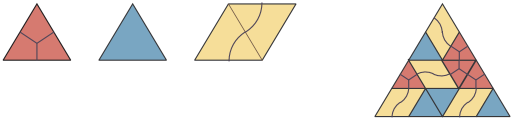
Figure 6.1. Tiles of the Knutson–Tao puzzles (up to rotation, reflections are not allowed), and an example of a puzzle.

6.13. Integer points

Let  $P\in\mathbb{R}^{d}$  be a rational convex H-polytope, i.e. defined by inequalities over $\mathbb{Q}$, and let  $\zeta(P)$  be the number of integer points in $P$. One can ask if  $\zeta$  is concise in full generality? Here we are assuming that the input is in unary. Note that  $\zeta$  is a counting function which generalizes the number of contingency tables (Example 5.4) and LR-coefficients (Example 5.3), but we don’t know if either of these is concise (see Conjectures 5.30 and 6.7).

There is a sneaky way to establish that  $\zeta$  is concise, by noting that in a special case this becomes one of the known  #P-complete problems in unary, with a parsimonious reduction from the  0/1 PERMANENT (see e.g. [DO04, Thm 1.2])  or the  #3SAT (see e.g. [IMW17, $\S$5.1] and references therein). Recall that both of these problems have concise counting functions. In both cases, Proposition 5.12 implies that  $\zeta$  is concise. We omit the details.

6.14. Domino tilings of simply connected regions

Recall that our proof of Theorem 3.1 uses regions that are not simply connected. Note also that Nadeau’s construction in Remark 3.2 is simply connected.

Conjecture 6.8.

Theorem 3.1 holds for simply connected regions.

If true, the proof would have to be much more elaborate than our proof for general regions. Indeed, note that domino tilings of simply connected regions have additional properties given by the height functions  (see e.g. [PST16, Rém04, Thu90]).

Additionally, the generalized Temperley’s bijection [KPW00] relates the number of domino tilings in simply connected regions with the number of spanning trees in certain grid graphs. Thus, Conjecture 6.8 can be reformulated to say that a certain restriction of  ${\rm st}$  is concise, see Example 5.21. This gives another reason to think that the conjecture might be difficult.

On the other hand, it follows from the approach [ÇS18, Sch19] and [CP24] that Conjecture 6.8 follows from Zaremba’s conjecture. Moreover, for the snake regions defined in [ÇS18] this approach gives the following analogue of (5.1); we omit the details.

Theorem 6.9.

There is  $c>1$, such that  $\mathcal{T}_{\text{\rm snake}}(n)\supseteq\big{\{}0,1,\ldots,c^{n/(\log n)}\big{\}}$, for all  $n\geq 1$.

6.15. Tilings with small tiles

The literature on tilings in the plane is much too large to be reviewed here, but let us mention a few relevant highlight. In [MR01], the authors proved NP-completeness for the decision problem and #P-completeness for the counting problem of tilings of general regions for a small set with just two tiles (up to rotation). In [BNRR95],  NP-completeness was proved for tilings with bars  $k\times 1$  and  $1\times k$, where  $k\geq 3$. This is especially remarkable since for the same set of tiles, tileability of simply connected regions is in P, see [KK93]. Finally, in [PY13b], a finite set of rectangle tiles was given, with an NP-complete decision problem and #P-complete corresponding counting problem for simply connected regions.

6.16. The induction two-step

The inductive arguments in the paper can be used to extend some results of concise functions. This phenomenon can be seen, for example, in Corollary 3.3 which arises naturally from the proof of Theorem 3.1. Similarly, for relatively prime  $(a,b)$, the analogue of the corollary holds for linear extensions of width two posets (Example 5.15), and the number of matchings of trees (Example 5.19). This is a corollary of properties of the Stern–Brocot tree (see references in [KS21]). Another notable example of this phenomenon is a beautiful result in [HKNS10], that for every two groups  $\Gamma_{0}$  and  $\Gamma_{1}$, there is a graph  $G=(V,E)$  and an edge  $e\in E$, such that  Aut$(G)=\Gamma_{0}$  and  Aut$(G-e)=\Gamma_{1}$ .

6.17. Concise functions

As we mentioned earlier, the notion of a concise function is closely related to  #P-completeness. Indeed, for every parsimonious reduction  $f\mapsto g$, if  $f$  is concise, then so is $g$. Below we give an example of a #P-complete function that is not  concise. Note that if either Conjecture 5.17 or Conjecture 6.1 is false, this would also give such examples.

On the other hand, note that there are several interesting examples of concise functions that are in FP, such as the number of spanning trees in simple graphs and the number of linear extensions of width two posets (Examples 5.21 and 5.15). This suggests that being concise is an interesting property in its own right, independently of complexity considerations.

6.18. Coincidence problems

Note that none of the natural #P-complete counting functions $f$ that we consider have the corresponding coincidence problems  C_f  in PH (unless PH collapses). Theorems 1.3 and 1.4 prove this in many cases, and some interesting examples remain open (see above). The same applies for the verification problem  V_f. Note that if  $f$  is recognizable, then these two problems are PH-equivalent, i.e.  $\text{\sc C}_{f}\in\textup{{{PH}}}\ \Longleftrightarrow\ \text{\sc V}_{f}\in\textup{{{PH}}}$  by the argument in the proof of Proposition 5.33.

The following elegant example by Greta Panova shows that #P-complete functions can have easy coincidence problems. In notation of $\S$4.4, let  $A=(a_{ij})\in\mathcal{M}_{n}$  where $\mathcal{M}_{n}$  is the set of $n\times n$  matrices with entries in  $\{0,1\}$. Denote  $g(A):=a_{11}+2a_{12}+4a_{13}+\ldots+2^{n^{2}-1}a_{nn}+2^{n^{2}}$  and let  $f:\sqcup\hskip 0.85355pt\mathcal{M}_{n}\to\mathbb{N}$  be defined by  $f(A):=\mathrm{per}(A)+2^{n^{2}}g(A)$. Observe that  $\mathrm{per}(A)\leq n!<2^{n^{2}}$. Since  $f(A)=\mathrm{per}(A)\mod 2^{n^{2}}$, we conclude that computing $\hskip 0.85355ptf\hskip 0.85355pt$ is  #P-complete. On the other hand, we have  $f(A)=f(A^{\prime})$  if and only if  $A=A^{\prime}$, so  C${}_{f}\in\textup{{{P}}}$.

Curiously, function  $f$  is not  almost complete since the first  $(n^{2}+1)$  bits determine the last  $n^{2}$  bits, but is concise since  $n^{2}=O\big{(}\log f(A)\big{)}$  for all  $A\in\mathcal{M}_{n}$ . Function  $f$  is not recognizable, however, since the corresponding restricted verification problem is exactly  V${}_{\text{PER}}$  which is not in PH (unless PH collapses). Now take  $\mathcal{M}_{n}^{\prime}:=\mathcal{M}_{n}\times[n]$. Define  $f^{\prime}(A,\ell):=f(A)$  if  $\ell=0$, and  $f^{\prime}(A,\ell):=\ell-1$  if  $\ell>0$. Then function  $f^{\prime}$  is complete, and thus not  concise. Of course, computing  $f^{\prime}$  remains  #P-complete.

This leaves us with more questions than answers. Is  C${}_{\text{PER}}\in\textup{{{coNP}}}$-hard? Is it  C₌P-complete under Turing reductions? What about other natural coincidence problems that we discuss in this paper? Does it make sense to consider a complexity class of  #P-complete recognizable functions as in Proposition 5.33?

6.19. Equality conditions

The equality conditions for many combinatorial inequalities, have been studied widely in the area, especially in order theory. We refer to [Gra83, Win86] for dated surveys, to [Pak22] for a recent overview. Computationally, the equality conditions are decision problems in  C₌P. This paper grew out of our efforts to understand the Alexandrov–Fenchel inequality for mixed volumes [CP23].

Acknowledgements

We are grateful to Karim Adiprasito, Sasha Barvinok, Richard Brualdi, Jesús De Loera, Darij Grinberg, Christian Ikenmeyer, Mark Jerrum, Nathan Kaplan, Greg Kuperberg, Alejandro Morales, Steven Noble, Greta Panova, Fedya Petrov, Colleen Robichaux, Rikhav Shah, David Soukup, Richard Stanley and Bridget Tenner, for useful discussions and helpful remarks. Special thanks to Noah Kravitz, Ashwin Sah and Richard Stong for their help explaining [KS21] and [Sto22].

This paper was finished when both authors were visiting the American Institute of Mathematics at their new location in Pasadena, CA. We are grateful to AIM for the hospitality. The first author was partially supported by the Simons Foundation. Both authors were partially supported by the NSF.

References

- [AB09] Sanjeev Arora and Boaz Barak, Computational complexity. A modern approach, Cambridge Univ. Press, Cambridge, 2009, 579 pp.
- [AS13] Jernej Azarija and Riste Škrekovski, Euler’s idoneal numbers and an inequality concerning minimal graphs with a prescribed number of spanning trees, Math. Bohem. 138 (2013), 121–131.
- [Bar17] Alexander Barvinok, Counting integer points in higher-dimensional polytopes, in Convexity and concentration, Springer, New York, 2017, 585–612.
- [BNRR95] Danièle Beauquier, Maurice Nivat, Éric Remila and Mike Robson, Tiling figures of the plane with two bars, Comput. Geom. 5 (1995), 1–25.
- [Ber85] Claude Berge, Graphs (second ed.), North-Holland, Amsterdam, 1985, 413 pp.
- [BJS93] Sara C. Billey, William Jockusch and Richard P. Stanley, Some combinatorial properties of Schubert polynomials, J. Algebraic Combin. 2 (1993), 345–374.
- [BBL98] Prosenjit Bose, Jonathan F. Buss and Anna Lubiw, Pattern matching for permutations, Inform. Process. Lett. 65 (1998), 277–283.
- [BLP23] Petter Brändén, Jonathan Leake and Igor Pak, Lower bounds for contingency tables via Lorentzian polynomials, Israel J. Math. 253 (2023), 43–90.
- [BC72] Joel Brenner and Larry Cummings, The Hadamard maximum determinant problem, Amer. Math. Monthly 79 (1972), 626–630.
- [BW91] Graham Brightwell and Peter Winkler, Counting linear extensions, Order 8 (1991), 225–247.
- [BEHO21] Patrick Browne, Ronan Egan, and Fintan Hegarty and Padraig Ó Catháin, A survey of the Hadamard maximal determinant problem, Electron. J. Combin. 28 (2021), no. 4, Paper No. 4.41, 35 pp.
- [BN65] Richard A. Brualdi and Morris Newman, Some theorems on the permanent, J. Res. Nat. Bur. Standards, Sect. B 69B (1965), 159–163.
- [ÇS18] Ilke Çanakçı and Ralf Schiffler, Cluster algebras and continued fractions, Compos. Math. 154 (2018), 565–593.
- [CP23] Swee Hong Chan and Igor Pak, Equality cases of the Alexandrov–Fenchel inequality are not in the polynomial hierarchy, preprint (2023), 35 pp.; arXiv:2309.05764; extended abstract to appear in Proc. 56th STOC, ACM, New York, 2024.
- [CP24] Swee Hong Chan and Igor Pak, Linear extensions and continued fractions, preprint (2024), 14 pp.; arXiv:2401.09723.
- [CP19] Danila Cherkashin and Fëdor Petrov, On small -uniform hypergraphs with positive discrepancy, J. Combin. Theory, Ser. B 139 (2019), 353–359.
- [CP18] Scott Corry and David Perkinson, Divisors and sandpiles. An introduction to chip-firing, AMS, Providence, RI, 2018, 325 pp.
- [Cra08] David A. Craven, Symmetric group character degrees and hook numbers, Proc. LMS 96 (2008), 26–50.
- [DL92] Paul Dagum and Michael Luby, Approximating the permanent of graphs with large factors, Theoret. Comput. Sci. 102 (1992), 283–305.
- [DO04] Jesús A. De Loera and Shmuel Onn, The complexity of three-way statistical tables, SIAM J. Comput. 33 (2004), 819–836.
- [DRS10] Jesús A. De Loera, Jörg Rambau and Francisco Santos, Triangulations, Springer, Berlin, 2010, 535 pp.
- [DP18] Samuel Dittmer and Igor Pak, Counting linear extensions of restricted posets, preprint (2018), 34 pp.; arXiv:1802.06312.
- [Epp20] David Eppstein, Counting polygon triangulations is hard, Discrete Comput. Geom. 64 (2020), 1210–1234.
- [EG61] Paul Erdős and Tibor Gallai, Graphs with prescribed degrees of vertices (in Hungarian), Mat. Lapok 11 (1961), 264–274.
- [GJ78] Michael R. Garey and David S. Johnson, “Strong” NP-completeness results: motivation, examples, and implications, J. ACM 25 (1978), 499–508.
- [GJ79] Michael R. Garey and David S. Johnson, Computers and Intractability: A Guide to the Theory of NP-completeness, Freeman, San Francisco, CA, 1979, 338 pp.
- [For97] Lance Fortnow, Counting complexity, in Complexity theory retrospective II, Springer, New York, 1997, 81–107.
- [GN06] Omer Giménez and Marc Noy, On the complexity of computing the Tutte polynomial of bicircular matroids, Combin. Probab. Comput. 15 (2006), 385–395.
- [GN09] Omer Giménez and Marc Noy, Asymptotic enumeration and limit laws of planar graphs, J. Amer. Math. Soc. 22 (2009), 309–329.
- [GK20] Darren Glass and Nathan Kaplan, Chip-firing games and critical groups, in A project-based guide to undergraduate research in mathematics, Springer, Cham, 2020, 107–152.
- [Gol08] Oded Goldreich, Computational complexity. A conceptual perspective, Cambridge Univ. Press, Cambridge, UK, 2008, 606 pp.
- [Gra83] Ronald L. Graham, Applications of the FKG inequality and its relatives, in Mathematical programming: the state of the art, Springer, Berlin, 1983, 115–131.
- [Gre93] Frederic Green, On the power of deterministic reductions to C=P, Math. Systems Theory 26 (1993), 215–233.
- [Gri14] Rostislav Grigorchuk, Milnor’s problem on the growth of groups and its consequences, in Frontiers in complex dynamics, Princeton Univ. Press, Princeton, NJ, 2014, 705–773.
- [Gri76] Geoffrey R. Grimmett, An upper bound for the number of spanning trees of a graph, Discrete Math. 16 (1976), 323–324.
- [Gro93] Helmut Groemer, Stability of geometric inequalities, in Handbook of convex geometry, Vol. A, North-Holland, Amsterdam, 1993, 125–150.
- [GT18] Alexander E. Guterman and Konstantin A. Taranin, On the values of the permanent of -matrices, Linear Algebra Appl. 552 (2018), 256–276.
- [Guy88] Richard K. Guy, The strong law of small numbers, Amer. Math. Monthly 95 (1988), 697–712.
- [HKNS10] Stephen G. Hartke, Hannah Kolb, Jared Nishikawa and Derrick Stolee, Automorphism groups of a graph and a vertex-deleted subgraph, Electron. J. Combin. 17 (2010), no. 1, RP 134, 8 pp.
- [IMW17] Christian Ikenmeyer, Ketan D. Mulmuley and Michael Walter, On vanishing of Kronecker coefficients, Comp. Complexity 26 (2017), 949–992.
- [IP22] Christian Ikenmeyer and Igor Pak, What is in #P and what is not?, preprint (2022), 82 pp.; extended abstract in Proc. 63rd FOCS (2022), 860–871; arXiv:2204.13149.
- [IPP22] Christian Ikenmeyer, Igor Pak and Greta Panova, Positivity of the symmetric group characters is as hard as the polynomial time hierarchy, preprint (2022), 15 pp.; extended abstract in Proc. 34th SODA (2023), 3573–3586; arXiv:2207.05423.
- [Jer87] Mark Jerrum, Two-dimensional monomer-dimer systems are computationally intractable. J. Statist. Phys. 48 (1987), 121–134. Erratum, 59 (1990), 1087–1088.
- [Jer94] Mark Jerrum, Counting trees in a graph is #P-complete, Inform. Process. Lett. 51 (1994), 111–116.
- [Jer06] Mark Jerrum, Two remarks concerning balanced matroids, Combinatorica 26 (2006), 733–742.
- [KK93] Claire Kenyon and Richard Kenyon, Comment paver des polygones avec des barres (in French), C. R. Acad. Sci. Paris, Sér. I Math. 316 (1993), no. 12, 1319–1322; Extended abstract: Tiling a polygon with rectangles, in Proc. 33rd FOCS (1992), 610–619.
- [Ken04] Richard Kenyon, An introduction to the dimer model, in ICTP Lect. Notes XVII, Trieste, 2004, 267–304.
- [KPW00] Richard Kenyon, James G. Propp, and David B. Wilson, Trees and matchings, Electron. J. Combin. 7 (2000), RP 25, 34 pp.
- [Kit11] Sergey Kitaev, Patterns in permutations and words, Springer, Heidelberg, 2011, 494 pp.
- [KR75] Daniel J. Kleitman and Bruce L. Rothschild, Asymptotic enumeration of partial orders on a finite set, Trans. AMS 205 (1975), 205–220.
- [Kli19] Caroline J. Klivans, The mathematics of chip-firing, CRC Press, Boca Raton, FL, 2019, 295 pp.
- [KN23] Christopher Knapp and Steven Noble, The complexity of the greedoid Tutte polynomial, preprint (2023), 44 pp.; arXiv:2309.04537.
- [Knu98] Donald E. Knuth, The art of computer programming. Vol. 2. Seminumerical algorithms (Third ed.), Addison-Wesley, Reading, MA, 1998, 762 pp.
- [Knu23] Allen Knutson, Schubert calculus and quiver varieties, Proc. ICM (2022, virtual), Vol. VI, 4582–4605, EMS Press, Berlin, 2023; available at tinyurl.com/5n99dbja
- [KS21] Noah Kravitz and Ashwin Sah, Linear extension numbers of -element posets, Order 38 (2021), 49–66.
- [KO12] Daniela Kühn and Deryk Osthus, A survey on Hamilton cycles in directed graphs, European J. Combin. 33 (2012), 750–766.
- [LP09] László Lovász and Michael D. Plummer, Matching theory, AMS, Providence, RI, 2009.
- [Mac95] Ian G. Macdonald, Symmetric functions and Hall polynomials (Second ed.), Oxford U. Press, New York, 1995, 475 pp.
- [Man01] Laurent Manivel, Symmetric functions, Schubert polynomials and degeneracy loci, SMF/AMS, Providence, RI, 2001, 167 pp.
- [Moon68] John W. Moon, Topics on tournaments, Holt, Rinehart and Winston, New York, 1968, 104 pp.; available at www.gutenberg.org/ebooks/42833
- [MM11] Cristopher Moore and Stephan Mertens, The nature of computation, Oxford Univ. Press, Oxford, UK, 2011, 985 pp.
- [MR01] Cristopher Moore and John M. Robson, Hard tiling problems with simple tiles, Discrete Comput. Geom. 26 (2001), 573–590.
- [MPP19] Alejandro H. Morales, Igor Pak and Greta Panova, Hook formulas for skew shapes III. Multivariate and product formulas, Algebraic Comb. 2 (2019), 815–861.
- [PA95] János Pach and Pankaj K. Agarwal, Combinatorial geometry, John Wiley, New York, 1995, 354 pp.
- [Pak22] Igor Pak, What is a combinatorial interpretation?, in Open Problems in Algebraic Combinatorics, AMS, Providence, RI, to appear, 58 pp.; arXiv:2209.06142.
- [PP20] Igor Pak and Greta Panova, Bounds on Kronecker coefficients via contingency tables, Linear Algebra Appl. 602 (2020), 157–178.
- [PP22] Igor Pak and Greta Panova, Durfee squares, symmetric partitions and bounds on Kronecker coefficients, J. Algebra 629 (2023), 358–380.
- [PPY19] Igor Pak, Greta Panova and Damir Yeliussizov, On the largest Kronecker and Littlewood–Richardson coefficients, J. Combin. Theory, Ser. A 165 (2019), 44–77.
- [PST16] Igor Pak, Adam Sheffer and Martin Tassy, Fast domino tileability, Discrete Comput. Geom. 56 (2016), 377–394.
- [PV10] Igor Pak and Ernesto Vallejo, Reductions of Young tableau bijections, SIAM J. Discrete Math. 24 (2010), 113–145.
- [PY13a] Igor Pak and Jed Yang, The complexity of generalized domino tilings, Electron. J. Comb. 20 (2013), no. 4, Paper 12, 23 pp.
- [PY13b] Igor Pak and Jed Yang, Tiling simply connected regions with rectangles, J. Combin. Theory, Ser. A 120 (2013), 1804–1816.
- [Pan23] Greta Panova, Computational complexity in algebraic combinatorics, to appear in Current Developments in Mathematics 2023, International Press, Boston, MA, 30 pp.; arXiv:2306.17511.
- [Pap94] Christos H. Papadimitriou, Computational Complexity, Addison-Wesley, Reading, MA, 1994, 523 pp.
- [PB83] J. Scott Provan and Michael O. Ball, The complexity of counting cuts and of computing the probability that a graph is connected, SIAM J. Comput. 12 (1983), 777–788.
- [RT10] Kári Ragnarsson and Bridget E. Tenner, Obtainable sizes of topologies on finite sets, J. Combin. Theory, Ser. A 117 (2010), 138–151.
- [Ras04] Etienne Rassart, A polynomiality property for Littlewood–Richardson coefficients, J. Combin. Theory, Ser. A 107 (2004), 161–179.
- [Rém04] Eric Rémila, The lattice structure of the set of domino tilings of a polygon, Theoret. Comput. Sci. 322 (2004), 409–422.
- [Sch78] Thomas J. Schaefer, The complexity of satisfiability problems, in Proc. 10th STOC, ACM, New York, 1978, 216–226.
- [Sch19] Rolf Schiffler, Snake graphs, perfect matchings and continued fractions, in Snapshots of modern mathematics from Oberwolfach, 2019, No 1, 10 pp; available at publications.mfo.de/handle/mfo/1405
- [Sch90] Uwe Schöning, The power of counting, in Complexity theory retrospective, Springer, New York, 1990, 204–223.
- [Sed70] Jiří Sedláček, On the minimal graph with a given number of spanning trees, Canad. Math. Bull. 13 (1970), 515–517.
- [Shah22] Rikhav Shah, Determinants of binary matrices achieve every integral value up to , Linear Algebra Appl. 645 (2022), 229–236.
- [SH91] Gerard Sierksma and Han Hoogeveen, Seven criteria for integer sequences being graphic, J. Graph Theory 15 (1991), 223–231.
- [OEIS] Neil J. A. Sloane, The online encyclopedia of integer sequences, oeis.org
- [Sno12] Michael Snook, Counting bases of representable matroids, Electron. J. Combin. 19 (2012), no. 4, Paper 41, 11 pp.
- [Sta10] Richard P. Stanley, A survey of alternating permutations, in Combinatorics and graphs, AMS, Providence, RI, 2010, 165--196.
- [Sta12] Richard P. Stanley, Enumerative Combinatorics, vol. 1 (second ed.) and vol. 2, Cambridge Univ. Press, Cambridge, UK, 2012, 626 pp., and 1999, 581 pp.
- [Ste14] John Stembridge, Generalized stability of Kronecker coefficients, preprint (2014), 27 pp.; available at tinyurl.com/429pkka3
- [Sto22] Richard Stong, Minimal graphs with a prescribed number of spanning trees, Australas. J. Combin. 82 (2022), 182--196.
- [Tar91] Jun Tarui, Randomized polynomials, threshold circuits, and the polynomial hierarchy, in Proc. 8th STACS (1991), 238--250.
- [Ten09] Bridget E. Tenner, Optimizing linear extensions, SIAM J. Discrete Math. 23 (2009), 1450--1454.
- [Thu90] William P. Thurston, Conway’s tiling groups, Amer. Math. Monthly 97 (1990), 757--773.
- [Toda91] Seinosuke Toda, PP is as hard as the polynomial-time hierarchy, SIAM J. Comput. 20 (1991), 865--877.
- [Tro95] William T. Trotter, Partially ordered sets, in Handbook of combinatorics, vol. 1, Elsevier, Amsterdam, 1995, 433--480.
- [Vad01] Salil P. Vadhan, The complexity of counting in sparse, regular, and planar graphs, SIAM J. Comput. 31 (2001), 398--427.
- [Val79a] Leslie G. Valiant, The complexity of enumeration and reliability problems, SIAM J. Comp. 8 (1979), 410--421.
- [Val79b] Leslie G. Valiant, Completeness classes in algebra, in Proc. 11th STOC (1979), 249--261.
- [Val79c] Leslie G. Valiant, The complexity of computing the permanent, Theoret. Comput. Sci. 8 (1979), 189--201.
- [Vat15] Vincent Vatter, Permutation classes, in Handbook of enumerative combinatorics, CRC Press, Boca Raton, FL, 2015, 753--833.
- [Wel93] Dominic J. A. Welsh, Complexity: knots, colourings and counting, Cambridge Univ. Press, Cambridge, UK, 1993, 163 pp.
- [Wig19] Avi Wigderson, Mathematics and computation, Princeton Univ. Press, Princeton, NJ, 2019, 418 pp.; available at math.ias.edu/avi/book
- [Win86] Peter M. Winkler, Correlation and order, in Combinatorics and ordered sets, AMS, Providence, RI, 1986, 151--174.
- [Wor18] Nicholas Wormald, Asymptotic enumeration of graphs with given degree sequence, in Proc. ICM Rio de Janeiro, Vol. 3, 2018, 3229--3248.