The boundary of Rauzy fractal and discrete tilings

Abstract.

The Rauzy fractal is a domain in the two-dimensional plane constructed by the Rauzy substitution, a substitution rule on three letters. The Rauzy fractal has a fractal-like boundary, and the currently known its constructions is not only for its boundary but also for the entire domain. In this paper, we show that all points in the Rauzy fractal have a layered structure. We propose two methods of constructing the Rauzy fractal using layered structures. We show how such layered structures can be used to construct the boundary of the Rauzy fractal with less computation than conventional methods. There is a self-replicating pattern in one of the layered structure in the Rauzy fractal. We introduce a notion of self-replicating word and visualize how some self-replicating words on three letters creates discrete tiling of the two dimensional plane.

Key words. Rauzy fractal, fractal boundary, discrete tiling

1. Introduction

In [9], Rauzy proposed a method of constructing a compact region called the Rauzy fractal (Figure 1(a)). There are two characteristics in the Rauzy fractal. One is that the Rauzy fractal has a fractal-like boundary (as its name indicates), and another is that it discretely tiles the two-dimensional plane (Figure 1(b)). The tiling characteristic of the Rauzy fractal generalizes to the Pisot conjecture, which states that every Pisot substitution ($\S\ref{sec:rauzy-fractal}$) on $d$ letters gives a discrete tiling of the $d$-dimensional space $\mathbb{R}^{d}$ [2, 3, 6, 10, 13]. Pisot substitutions are also studied in relationship with Pisot numbers [7, 14]. In symbolic dynamics, Pisot substitution plays one of key role in understanding the substitutive systems [1, 8]. Pisot conjecture further generalizes to the pure discrete spectrum conjecture which states that every dynamical system defined by a Pisot substitution on $d$ letters has a pure discrete spectrum, which has been proved only for $d\leq 2$ [4, 5, 11, 12].

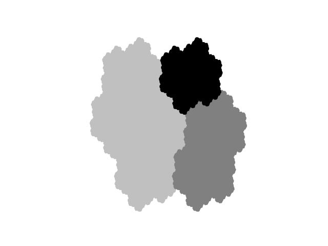
(a) Rauzy fractal in three colors.

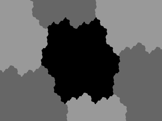
(b) Tiling of the Rauzy fractal

Figure 1. The Rauzy fractal and its tiling

There are two ways known to construct Rauzy fractal. One uses a convergent sequence of $3$-dimensional points [9], and the other uses the exductive method [2]. Both methods construct the entire Rauzy fractal, and increase the resolution of the Rauzy fractal with larger computations for its boundary and interior at the same time. Since the Rauzy fractal is a simply connected domain, so the higher resolution is only visible on its boundary. So it is questionable whether we can effectively increase the resolution of the boundary of the Rauzy fractal only.

Our main goal is to find an efficient algorithm for drawing the boundary of the Rauzy fractal. We found two new construction methods for the Rauzy fractal. Both methods rely on the fact that Rauzy fractal is the union of “layered” points. The first method, the construction A ($\S\ref{sec:rauzy-const-1}$) uses Theorem 1, which states that the union of all A-layers (Equations (26) - (29)) is the Rauzy fractal. To define the points in the A-layers, we use the tribonacci words (c.f. Equation (14)). Each A-layer has its level, and the points in the A-layers at the same level cluster into hexagons, called cells. Thus we can visualize the boundary of the Rauzy fractal with the boundary cells (c.f. Figures 4).

The second method, the construction B ($\S\ref{sec_alternative_construction}$) uses Theorem 2, which states that the union of all B-layers is the Rauzy fractal. The B-layers are defined by a pseudo-self-replicating pattern in the sequence of $0102010$ (Equations (76) - (82)). The points in the B-layers are determined only by this pattern, whereas the points in the A-layers requires extra information on tribonacci words. The word “pseudo” comes from the exception at the number $2$ in the sequence $0102010$, which we must have in order to create the exact Rauzy fractal. Interestingly, we still get compact domains when we use fullly self-replicating patterns of various sequence. In $\S\ref{sec_discrete_tiling_plane}$, we will visualize certain patterns that create compact domains which tiles $\mathbb{R}^{2}$ discretely (Figures 7, 8(a)).

2. Pisot substitutions and their domains

Let the letters be the integers $0,1,2,\cdots$, and a word be a string of letters. Given a sequence $\mathbf{w}=(w_{0},\cdots,w_{l})$ of integers, we denote a word $[\mathbf{w}]$ as

(1) $$[\mathbf{w}]=[w_{0}w_{1}\cdots w_{l}].$$

We call each $w_{i}$ a character. A word on $d$ letters is a word whose characters are in the $d$ letters from $0$ to $d-1$. The empty word is the word without any character, and denoted by $[\,]$. The length of the word is the number of its characters. For example, $L([\,])=0$ and $L([w_{0}\cdots w_{l}])=l+1$. Given a word $[\mathbf{w}]$ on $d$ letters, the word vector for $[w]$ is the $d$-dimensional (integral) vector whose $(i+1)$-th entry ($i=0,\cdots,d-1$) is the number of the letter $i$ in the characters of $[\mathbf{w}]$. The following shows few examples of words $[\mathbf{w}_{n}]$ and their word vectors $\mathbf{v}_{n}$

(2) $$[\mathbf{w}_{0}] =[0], \mathbf{v}_{0}=(1,0,0),$$

(3) $$[\mathbf{w}_{1}] =[01], \mathbf{v}_{1}=(1,1,0),$$

(4) $$[\mathbf{w}_{2}] =[0102], \mathbf{v}_{2}=(2,1,1),$$

(5) $$[\mathbf{w}_{3}] =[0102010], \mathbf{v}_{3}=(4,2,1),$$

(6) $$[\mathbf{w}_{4}] =[0102010010201],\quad \mathbf{v}_{4}=(7,4,2).$$

A subword of $[w_{0}\cdots w_{l}]$ is a substring of the form $[w_{0}\cdots w_{l^{\prime}}]$, $0\leq l^{\prime}\leq l$. For example, from Equations (2) - (6), $[\mathbf{w}_{i}]$ is a subword for $[\mathbf{w}_{j}]$ for $i<j$. We consider the empty word as a subword of any word. We can concatenate words to make another word. For example, from Equations (2) - (5),

(7) $$[\mathbf{w}_{3}]=[\mathbf{w}_{2}][\mathbf{w}_{1}][\mathbf{w}_{0}]=[0102010].$$

A substitution on $d$ letters is a map that transforms single-character words $[0],\cdots,[d-1]$ to words on $d$ letters. For example, $\sigma_{i}$, $i=0,1,2,3$, defined below are substitutions on $3$ letters:

(8) $$\sigma_{0}([0])=[01], \sigma_{0}([1])=[02],\quad \sigma_{0}([2])=[0]$$

(9) $$\sigma_{1}([0])=[12], \sigma_{1}([1])=[2], \sigma_{1}([2])=[0]$$

(10) $$\sigma_{2}([0])=[0102],\quad \sigma_{1}([1])=[2], \sigma_{1}([2])=[0]$$

(11) $$\sigma_{3}([0])=[01], \sigma_{2}([1])=[2], \sigma_{2}([2])=[0]$$

A substitution can transforms any words as follows

(12) $$\sigma([w_{0}\cdots w_{l}])=\sigma([w_{0}])\cdots\sigma([w_{l}]).$$

With the initial word $[\mathbf{w}_{0}]=[0]$, any substitution $\sigma$ generates the sequence of words $[\mathbf{w}_{n}]$ recursively as follows.

(13) $$[\mathbf{w}_{n+1}]=\sigma([\mathbf{w}_{n}])\textrm{ for }n\geq 0.$$

For example, $[\mathbf{w}_{n}]$, $n=0,\cdots,4$, in Equations (2) - (6) are the first five sequence generated by the substitution $\sigma_{0}$ in Equation (8). The substitution $\sigma_{0}$ in Equation (8) is called the Rauzy substitution. The sequence of words $[\mathbf{w}_{n}]$ in Equation (13) obtained by the Rauzy substitution is called the tribonacci words. Let us denote the tribonacci words as $[\mathbf{a}_{n}]$ to distinguish them from general notation for words The tribonacci words satisfies the following recursive formula.

(14) $$[\mathbf{a}_{n+3}]=[\mathbf{a}_{n+2}][\mathbf{a}_{n+1}][\mathbf{a}_{n}]\textrm{ for }n\geq 0.$$

Let $\mathbf{v}_{n}$ be the word vector for the word $[\mathbf{w}_{n}]$ in Equation (13). We can associate a unique $d\times d$ matrix $M$ for each substitution $\sigma$ that satisfies

(15) $$\mathbf{v}_{n+1}=M\mathbf{v}_{n}\textrm{ for }n\geq 0$$

A $d\times d$ matrix $M$ is called a Pisot matrix if its characteristic polynomial has a unique real root $\lambda$ greater than $1$ and all the other (complex) roots have absolute values less than $1$. A substitution $\sigma$ is called a Pisot substitution if the corresponding matrix $M$ in Equation (15) is a Pisot matrix. The unique real root $\lambda$ is called a Pisot number.

Pisot substitution	Pisot matrix	characteristic polynomial	Pisot number
$\sigma_{0}$	$\begin{bmatrix}1&1&1\\ 1&0&0\\ 0&1&0\end{bmatrix}$	$1+\lambda+\lambda^{2}=\lambda^{3}$	$1.8393$
$\sigma_{1}$	$\begin{bmatrix}0&1&1\\ 0&0&1\\ 1&0&0\end{bmatrix}$	$1+\lambda=\lambda^{3}$	$1.3247$
$\sigma_{2}$	$\begin{bmatrix}2&1&1\\ 0&0&1\\ 1&0&0\end{bmatrix}$	$1+\lambda+2\lambda^{2}=\lambda^{3}$	$2.5468$
$\sigma_{3}$	$\begin{bmatrix}1&1&0\\ 0&0&1\\ 1&0&0\end{bmatrix}$	$1+\lambda^{2}=\lambda^{3}$	$1.4656$

Table 1. Matrices associated with Pisot substitution

Table 1 shows the Pisot matrix and Pisot number for the substitutions $\sigma_{i}$ in Equation (8) - (11). The Pisot matrix has a real eigenvector $\mathbf{v}_{\infty}$ whose eigenvalue is the Pisot number $\lambda$.

(16) $$M\mathbf{v}_{\infty}=\lambda\mathbf{v}_{\infty}.$$

Indeed, the limit $\lim\mathbf{v}_{n}/\|\mathbf{v}_{n}\|$ is the eigenvector with the eigenvalue $\lambda$, where $\mathbf{v}_{n}$ is the word vector for $[\mathbf{w}_{n}]$ in Equation (13). The hyperplane $P$ in $\mathbb{R}^{d}$ orthogonal to $\mathbf{v}_{\infty}$ is call the contracting plane. For each $[\mathbf{w}_{n}]$, let $\mathbf{v}_{l}$ be the word vector for the subword of $[\mathbf{w}_{n}]$ with the length $l$. Let $\pi:\mathbb{R}^{d}\to P$ be the orthogonal projection and define the set $R_{n}$ as

(17) $$R_{n}=\{\mathbf{0}\}\cup\{\pi(\mathbf{v}_{l})\,|\,0\leq l\leq L\}.$$

We will call the set $R=\displaystyle\bigcup_{n=0}^{\infty}R_{n}$ the Pisot domain for $\sigma$.

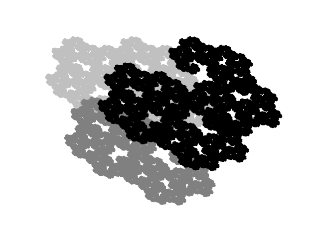
(a) The Pisot domain for $\sigma_{1}$

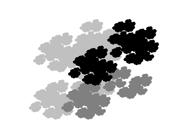
(b) The Pisot domain for $\sigma_{2}$

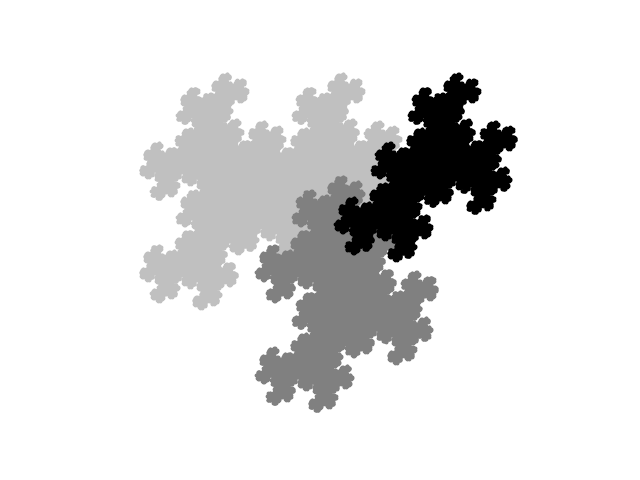
(c) The Pisot domain for $\sigma_{3}$

Figure 2. Pisot domains for Pisot substitutions in three colors.

Figure 1(a) is the Pisot domain for the Rauzy substitution $\sigma_{0}$, and Figure 2 are the Pisot domains for the substitutions $\sigma_{i}$, $i=1,2,3$. Here we explain how to obtain such figures. Let

(18) $$\mathbf{e}_{0}=(1,0,0),\mathbf{e}_{1}=(0,1,0),\mathbf{e}_{2}=(0,0,1)$$

be the standard orthogonal basis for $\mathbb{R}^{3}$. We choose sufficiently long word $[\mathbf{w}_{n}]=[w_{0}\cdots w_{L}]$, and its word vector $\mathbf{v}_{n}$. We approximate $\mathbf{v}_{\infty}\approx\mathbf{v}_{n}$, to define the contracting plane $P$ to be the hyperbolic plane orthogonal to $\mathbf{v}_{n}$. (The size of $n$ is determined by how “dense” the figure obtained at the end looks.) We run the Gram–Schmidt process on the set $\{\mathbf{v}_{n}/\|\mathbf{v}_{n}\|,\mathbf{e}_{0},\mathbf{e}_{1}\}$ to obtain two orthonormal basis $\mathbf{r}_{0}$, $\mathbf{r}_{1}$ on $P$. For each subword $[w_{0}\cdots w_{l}]$, $0\leq l\leq L$, of $[\mathbf{w}_{n}]$, let $\mathbf{v}_{l}$ be its word vector, and define the $2$-dimensional vector $\mathbf{x}_{l}$ as follows.

(19) $$\mathbf{x}_{l}=(\pi(\mathbf{v}_{l})\cdot\mathbf{r}_{0},\pi(\mathbf{v}_{l})\cdot\mathbf{r}_{1}).$$

We then plot the dot at $\mathbf{x}_{l}$ for all $0\leq l\leq L$ with the color depending on the letter of the character $w_{l}$.

3. Rauzy fractal construction A

Our prime concern is to understand the Rauzy fractal (Figure 1(a)) and its boundary. We will consider the Rauzy substitution $\sigma_{0}$ only from now on. We will call a $2$-dimensional point $\mathbf{x}$ to be Rauzy if $\mathbf{x}\in R_{n}$ for some $n\geq 0$. Equation (14) implies that $R_{n}\subset R_{n+1}$. Thus we can identify Rauzy points by the lengths of corresponding subwords uniquely.

Let $\mathbf{e}_{0},\mathbf{e}_{1},\mathbf{e}_{2}$ be the standard basis on $\mathbb{R}^{3}$ defined in Equation (18). Let $\mathbf{u}_{0}$, $\mathbf{u}_{1}$, and $\mathbf{u}_{2}$ be the $2$-dimensional vectors defined by

(20) $$\mathbf{u}_{i}=(\pi(\mathbf{e}_{i})\circ\mathbf{r}_{0},\pi(\mathbf{e}_{i})\circ\mathbf{r}_{1}),\textrm{ for }i=0,1,2,$$

where $\mathbf{r}_{0},\mathbf{r}_{1}$ are orthonormal basis on the contracting plane $P$ for the Rauzy substitution.

Let $\mathbf{b}_{n}$ be the Rauzy point for the tribonacci words $[\mathbf{a}_{n}]$. The first four $\mathbf{b}_{n}$ are

(21) $$\mathbf{b}_{0} =\mathbf{u}_{0},$$

(22) $$\mathbf{b}_{1} =\mathbf{u}_{0}+\mathbf{u}_{1},$$

(23) $$\mathbf{b}_{2} =2\mathbf{u}_{0}+\mathbf{u}_{1}+\mathbf{u}_{2},$$

(24) $$\mathbf{b}_{3} =4\mathbf{u}_{0}+2\mathbf{u}_{1}+\mathbf{u}_{2},$$

(25) $$\mathbf{b}_{4} =7\mathbf{u}_{0}+4\mathbf{u}_{1}+2\mathbf{u}_{2}.$$

For a semantic reason, let us denote $\mathbf{b}_{i}^{(j)}=\mathbf{b}_{3i+j}$. The A-layer at the level $i$ is the set $V_{i}$ of Rauzy poitns defined inductively as follows:

(26) $$V_{-1} =\{\mathbf{0}\},\textrm{ and for }i\geq 0,$$

(27) $$V_{i}^{(0)} =\{\mathbf{x}+\mathbf{b}_{i}^{(0)}\,|\,\mathbf{x}\in\bigcup_{j=-1}^{i-1}V_{j}\},$$

(28) $$V_{i}^{(1)} =\{\mathbf{x}+\mathbf{b}_{i}^{(1)},\mathbf{x}+\mathbf{b}_{i}^{(0)}+\mathbf{b}_{i}^{(1)}\,|\,\mathbf{x}\in\bigcup_{j=-1}^{i-1}V_{j}\},$$

(29) $$V_{i}^{(2)} =\{\mathbf{x}+\mathbf{b}_{i}^{(2)},\mathbf{x}+\mathbf{b}_{i}^{(0)}+\mathbf{b}_{i}^{(2)},\mathbf{x}+\mathbf{b}_{i}^{(1)}+\mathbf{b}_{i}^{(2)}\,|\,\mathbf{x}\in\bigcup_{j=-1}^{i-1}V_{j}\},$$

(30) $$V_{i} =\bigcup_{j=0}^{2}V_{i}^{(j)}.$$

We have the following result.

Theorem 1.

The set of all Rauzy points is the union of all A-layers at all levels.

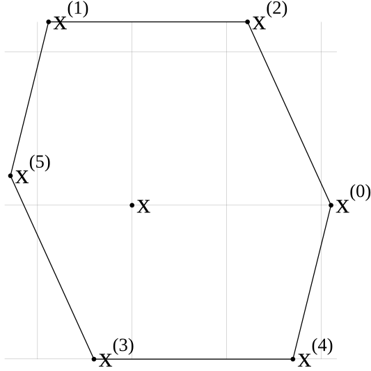
(a) The six children points $\mathbf{x}^{(j)}$ form a cell of their parent point $\mathbf{x}$.

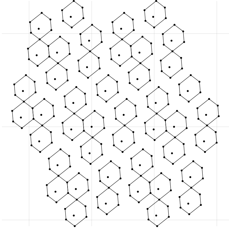
(b) The cells at each level are uniformly distributed.

Figure 3. Rauzy points in Rauzy fractal. The $x$, $y$-axis are equally scaled.

Before we prove the theorem, let us show how we can use this theorem to construct Rauzy fractal and its boundary. For any $\mathbf{x}\in V_{i-1}$, the following six points are in $V_{i}$:

(31) $$\mathbf{x}^{(0)} =\mathbf{x}+\mathbf{b}_{i}^{(0)} \in V_{i}^{(0)},$$

(32) $$\mathbf{x}^{(1)} =\mathbf{x}+\mathbf{b}_{i}^{(1)} \in V_{i}^{(1)},$$

(33) $$\mathbf{x}^{(2)} =\mathbf{x}+\mathbf{b}_{i}^{(0)}+\mathbf{b}_{i}^{(1)} \in V_{i}^{(1)},$$

(34) $$\mathbf{x}^{(3)} =\mathbf{x}+\mathbf{b}_{i}^{(2)} \in V_{i}^{(2)},$$

(35) $$\mathbf{x}^{(4)} =\mathbf{x}+\mathbf{b}_{i}^{(0)}+\mathbf{b}_{i}^{(2)} \in V_{i}^{(2)},$$

(36) $$\mathbf{x}^{(5)} =\mathbf{x}+\mathbf{b}_{i}^{(1)}+\mathbf{b}_{i}^{(2)} \in V_{i}^{(2)}.$$

These points forms a hexagon around $\mathbf{x}$ (Figure 3(a)). We will call this hexagon as the cell of $\mathbf{x}$. The point $\mathbf{x}^{(j)}$, $j=0,\cdots,5$, is a child of its parent $\mathbf{x}$. Theorem 1 implies that Rauzy fractal can be filled recursively by tracing the genealogy of the Rauzy points, starting from the origin $\mathbf{0}$. To plot the boundary of Rauzy fractal, we trace only the descendents that lie outside of the cells of their ancestors. These points are called the boundary points. (To speed up the computation, we can only check whether a points lie inside of the cell of its grandparent.) At each level of layers, we produce the children only for the boundary points, and they are clustered into cells that are uniformly distributed. Figure 3(b) shows all points in A-layers up to the level $3$. In fact, they are the first $274$ Rauzy points, including the origin. The cells are only drawn for the points in A-layer at the level $3$. The interior points in cells are all the points in A-layer up to the level $2$. We can see that there is no conflict on the geneology of points: no two points in the same level of A-layer never enjoy a child-parent relationship.

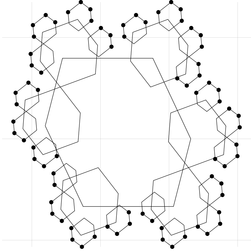
(a) The boundary points and cells up to the level $3$.

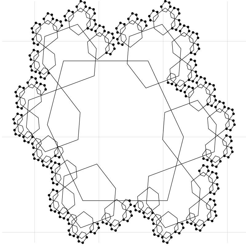
(b) The boundary points and cells up to the level $4$.

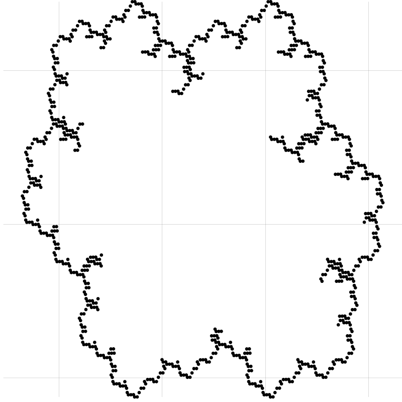
(c) The boundary points up to the layer $5$.

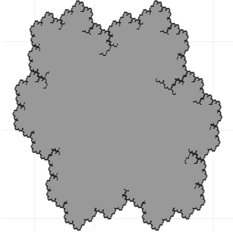
(d) The boundary of Rauzy fractal with its interior.

Figure 4. The boundary Rauzy points in A-layers and the cells.

Figure 4(a) shows the Rauzy points (filled-dots) in A-layers at the level $3$. The hexagons are the cells of boundary points in the previous layers. We can plot only the boundary points at each layer to determine the boundary of Rauzy fractal. Figure 3(b) shows all boundary points in the A-layer at the level $4$ and the cells of all boundary points in the previous layers. One can see that the boundary point at the top layer forms the boundary of the Rauzy fractal. Figure 4(c) shows the boundary points at the level $5$, and Figure 4(d) shows them with Rauzy fractal. One might wonder why there seems to be several estuaries (rivers that meet the ocean), if we put an analogy of Rauzy fractal as the “land” and its complement as an “ocean”. This phenomenon does not mean that the Rauzy fractal has a vacuous “valley”. It is a consequence of discarding non-boundary points at each level. To reduce the computational complexity, it is inevitable to disregard some cells when checking the interior points. As we observed in Figure 3(b), all Rauzy points are almost-uniformly distributed. The shape of the boundary of the Rauzy fractal in Figure 4(c) is optimal in our setting. To remove all estuaries, we should consider all cells at each level of A-layers. This is essentially the same as the conventional way of drawing the Rauzy fractal, and requires the same amount of computational complexity.

Let us prove Theorem 1. We will prove the following holds for all $i\geq 0$:

(37) $$V_{i}=R_{3i+3}-\{\mathbf{b}_{3i+3}\}.$$

Since every Rauzy point $\mathbf{x}_{l}$ is uniquely identified with the length of corresponding substring $[\mathbf{w}_{l}]$ of a tribonacci word, we define the length of the Rauzy point $\mathbf{x}_{l}$ as the length of its subword $[\mathbf{w}_{l}]$:

(38) $$L(\mathbf{x}_{l})=L([\mathbf{w}_{l}]).$$

The following lemma is the key to the proof of Equation (37).

Lemma.

If $\mathbf{x}$ is a Rauzy point satisfying

(39) $$L(\mathbf{x})\leq L(\mathbf{b}_{n-1})+L(\mathbf{b}_{n-2}),$$

then $\mathbf{x}+\mathbf{b}_{n}$ is also a Rauzy point.

Proof.

Let $[\mathbf{w}]$ be the word corresponding to the Rauzy point $\mathbf{x}$. From the condition of the lemma, $[\mathbf{w}]$ is a substring of the word $[\mathbf{a}_{n-1}][\mathbf{a}_{n-2}]$. Thus the word $[\mathbf{a}_{n}][\mathbf{w}]$ is a substring of $[\mathbf{a}_{n+1}]$, and it contains $[\mathbf{a}_{n}]$. Therefore $\mathbf{x}+\mathbf{b}_{n}$ is a Rauzy point. ∎

Let us prove Equation (37) by the induction. Obviously, $V_{-1}=R_{0}-\{\mathbf{b}_{0}\}=\{\mathbf{0}\}$. We get the first six Rauzy points by letting $\mathbf{x}=\mathbf{0}$ in Equations (31)-(36). Thus $V_{0}=R_{3}-\{\mathbf{b}_{3}\}$. This shows that Equation (37) holds for $i=-1,0$.

Let us assume that Equation (37) holds for $i-2$ and $i-1$ for $i\geq 1$. We will show that each set $V_{i}^{(j)}$ is a subset of $R_{3i+3}-\{\mathbf{b}_{3i+3}\}$, and all Rauzy points $\mathbf{x}$ satisfying $L(\mathbf{b}_{3i})\leq L(\mathbf{x})<L(\mathbf{b}_{3i+3})$ appears in one of $V_{i}^{(j)}$.

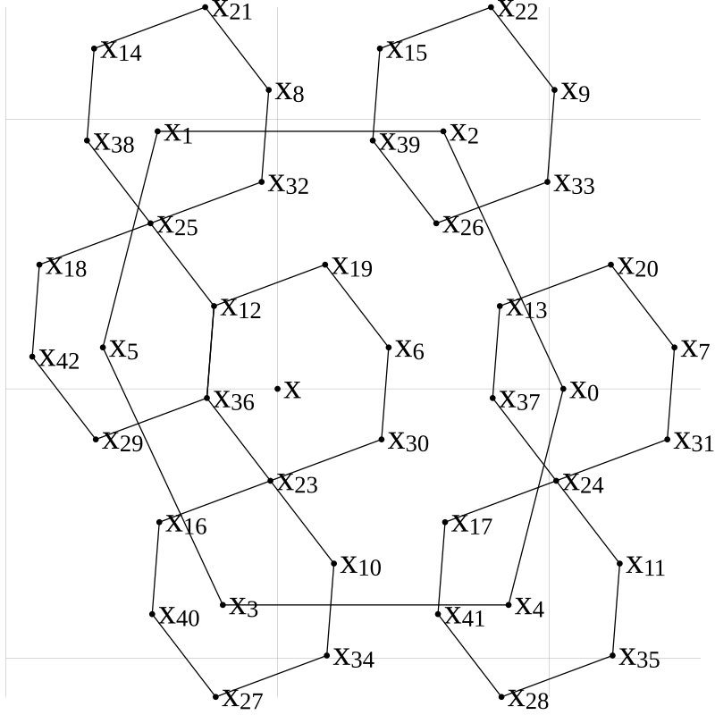
Figure 5. The first $43$ Rauzy points in A-layers up to the level $2$ are shown with numbered indices. The cells are represented by hexagons.

To help understanding, we will use Figure 5, which shows the first $51$ Rauzy points with the origin $\mathbf{x}$. It shows the general configurations of children and grand children of $\mathbf{x}$. We can see that some points have two parents. For any choice of $\mathbf{x}\in V_{i-2}$, the ancestries of all points are identical. The inclusions and exclusions of points to the cells of their ancesters may differ by the choice of $\mathbf{x}$, but our proof does not depend on it. We assume $\mathbf{x}\in V_{i-2}$ and $\mathbf{x}_{0},\cdots,\mathbf{x}_{5}\in V_{i-1}$ be the children of $\mathbf{x}$ obtained by Equations (31)-(36). We also assume that $\mathbf{x}_{0},\cdots,\mathbf{x}_{5}$ are Rauzy points. We will show that

(40) $$\mathbf{x}_{6},\cdots,\mathbf{x}_{12} \in V_{i}^{(0)},$$

(41) $$\mathbf{x}_{13},\cdots,\mathbf{x}_{25} \in V_{i}^{(1)},$$

(42) $$\mathbf{x}_{26},\cdots,\mathbf{x}_{42} \in V_{i}^{(2)}.$$

The points in Equation (40) are obtained by adding $\mathbf{b}_{i}^{(0)}$:

(43) $$\mathbf{x}_{6}=\mathbf{x}+\mathbf{b}_{i}^{(0)},\quad\mathbf{x}_{j+7}=\mathbf{x}_{j}+\mathbf{b}_{i}^{(0)}\textrm{ for }0\leq j\leq 5.$$

The assumption $\mathbf{x}\in V_{i-1}$ implies $L(\mathbf{x})<L(\mathbf{b}_{i-1}^{(0)})$. Thus we can use Equations (31)-(35) to show that $\mathbf{x}$ and $\mathbf{x}_{0},\cdots,\mathbf{x}_{4}$ satisfies the inequality (39):

(44) $$L(\mathbf{x}) <L(\mathbf{b}_{3i-3}) <L(\mathbf{b}_{3i-2}),$$

(45) $$L(\mathbf{x}_{0}) <L(\mathbf{b}_{3i-3})+L(\mathbf{b}_{3i-3}) <L(\mathbf{b}_{3i-1}),$$

(46) $$L(\mathbf{x}_{1}) <L(\mathbf{b}_{3i-3})+L(\mathbf{b}_{3i-2}) <L(\mathbf{b}_{3i-1}),$$

(47) $$L(\mathbf{x}_{2}) <L(\mathbf{b}_{3i-3})+L(\mathbf{b}_{3i-2})+L(\mathbf{b}_{3i-3}) <L(\mathbf{b}_{3i-1})+L(\mathbf{b}_{3i-2}),$$

(48) $$L(\mathbf{x}_{3}) <L(\mathbf{b}_{3i-3})+L(\mathbf{b}_{3i-1}) <L(\mathbf{b}_{3i-1})+L(\mathbf{b}_{3i-2}),$$

(49) $$L(\mathbf{x}_{4}) <L(\mathbf{b}_{3i-3})+L(\mathbf{b}_{3i-1})+L(\mathbf{b}_{3i-3}) \leq L(\mathbf{b}_{3i-1})+L([\mathbf{a}_{3i-2}]).$$

Therefore, $\mathbf{x}_{6},\cdots,\mathbf{x}_{11}$ are Rauzy points by the lemma. Equation (36) shows that

(50) $$L(\mathbf{x}_{5})\leq L(\mathbf{b}_{3i-6})+L(\mathbf{b}_{3i-1})+L(\mathbf{b}_{3i-2}).$$

This does not immediately imply the inequality (39). Meanwhile, $\mathbf{x}_{12}$ also satisfies

(51) $$\mathbf{x}_{12}=\mathbf{x}+\mathbf{b}_{i-1}^{(1)}+\mathbf{b}_{i-1}^{(2)}+\mathbf{b}_{i}^{(0)}=\mathbf{x}+\mathbf{b}_{i}^{(1)}.$$

Therefore $\mathbf{x}_{12}$ is also a Rauzy point by the lemma. The point $\mathbf{x}_{12}$ is the longest Rauzy point among its siblings. Since the longest length for $\mathbf{x}$ is $L(\mathbf{b}_{i-1}^{(0)})-1$,

(52) $$\max L(\mathbf{x}_{12})=L(\mathbf{b}_{i-1}^{(0)})+L(\mathbf{b}_{i}^{(1)})-1<L(\mathbf{b}_{i}^{(2)}).$$

Thus we proved that $V_{i}^{(0)}\subset R_{3i+2}\subset R_{3i+3}-\{\mathbf{b}_{3i+3}\}$.

Next, we show that points in Equation (41) are Rauzy points. On the other hands, they are obtained by adding $\mathbf{b}_{i}^{(1)}$ to the previous points:

(53) $$\mathbf{x}_{j+13}=\mathbf{x}_{j}+\mathbf{b}_{i}^{(1)},\quad 0\leq j\leq 12.$$

From Equations (32) - (33), we can easily check that

(54) $$L(\mathbf{x}_{j})\leq L(\mathbf{b}_{i-1}^{(2)})+L(\mathbf{b}_{i}^{(0)})\textrm{ for }0\leq j\leq 9.$$

However, this inequality is not immediate obvious for the following three points.

(55) $$L(\mathbf{x}_{10}) =L(\mathbf{x})+L(\mathbf{b}_{i-1}^{(2)})+L(\mathbf{b}_{i}^{(0)}),$$

(56) $$L(\mathbf{x}_{11}) =L(\mathbf{x})+L(\mathbf{b}_{i-1}^{(0)})+L(\mathbf{b}_{i-1}^{(2)})+L(\mathbf{b}_{i}^{(0)}),$$

(57) $$L(\mathbf{x}_{12}) =L(\mathbf{x})+L(\mathbf{b}_{i-1}^{(1)})+L(\mathbf{b}_{i-1}^{(2)})+L(\mathbf{b}_{i}^{(0)}).$$

In fact, these points are obtained by adding $\mathbf{b}_{i}^{(2)}$ to the previous Rauzy points.

(58) $$\mathbf{x}_{23} =\mathbf{x}+\mathbf{b}_{i}^{(2)},$$

(59) $$\mathbf{x}_{24} =\mathbf{x}+\mathbf{b}_{i-1}^{(0)}+\mathbf{b}_{i}^{(2)},$$

(60) $$\mathbf{x}_{25} =\mathbf{x}+\mathbf{b}_{i-1}^{(1)}+\mathbf{b}_{i}^{(2)}.$$

Therefore $\mathbf{x}_{23},\mathbf{x}_{24},\mathbf{x}_{25}$ are Rauzy points by the lemma. The maximum length of $\mathbf{x}_{25}$ is

(61) $$\max L(\mathbf{x}_{25})=L(\mathbf{b}_{i-1}^{(0)})+L(\mathbf{b}_{i-1}^{(1)})+L(\mathbf{b}_{i}^{(2)})-1,$$

and it is strictly less than $L(\mathbf{b}_{i+1}^{(0)})$. Thus $V_{i}^{(1)}\subset R_{3i+3}-\{\mathbf{b}_{3i+3}\}$.

Using Equations (34) - (36), we can apply the lemma to the points in Equation (42) without any exception. The maximum length of the longest Rauzy point is $\mathbf{x}_{42}$ is

$$\max L(\mathbf{x}_{42}) =L(\mathbf{b}_{i-1}^{(0)})+L(\mathbf{b}_{i-1}^{(1)})+L(\mathbf{b}_{i-1}^{(2)})+L(\mathbf{b}_{i}^{(1)})+L(\mathbf{b}_{i}^{(2)})-1$$

$$=L(\mathbf{b}_{i}^{(0)})+L(\mathbf{b}_{i}^{(1)})+L(\mathbf{b}_{i}^{(2)})-1$$

(62) $$=L(\mathbf{b}_{i+1}^{(0)})-1.$$

Therefore, $V_{i}^{(2)}\subset R_{3i+3}-\{\mathbf{b}_{3i+3}\}$.

So far, we showed that

(63) $$V_{i}^{(0)}\cup V_{i}^{(1)}\cup V_{i}^{(2)}\subset(R_{3i+3}-\{\mathbf{b}_{3i+3}\})-(R_{3i}-\{\mathbf{b}_{3i}\})$$

Let us show that the opposite holds too. First, suppose that $\mathbf{x}$ is a Rauzy point satisfying

(64) $$L(\mathbf{b}_{i}^{(0)})\leq L(\mathbf{x})<L(\mathbf{b}_{i}^{(1)}).$$

Then the word $[\mathbf{w}]$ corresponding to $\mathbf{x}$ is of the form

(65) $$[\mathbf{w}]=[\mathbf{a}_{3i}]\mathbf{[}\mathbf{w}^{\prime}]$$

where $[\mathbf{w}^{\prime}]$ is a substring of the word $[\mathbf{a}_{3i-1}][\mathbf{a}_{3i-2}]$. Therefore the word $[\mathbf{w}^{\prime}]$ is a subword in the tribonacci word $[\mathbf{a}_{3i}]$, and the corresponding Rauzy points $\mathbf{x}^{\prime}$ lies in $V_{i-1}$. Since Equation (65) implies

(66) $$\mathbf{x}=\mathbf{x}^{\prime}+\mathbf{b}_{i}^{(0)},$$

we havev $\mathbf{x}\in V_{i}^{(0)}$. This is the point $\mathbf{x}^{(0)}$ in Equation (31)

Next, suppose that $\mathbf{x}$ is a Rauzy point satisfying

(67) $$L(\mathbf{b}_{i}^{(1)})\leq L(\mathbf{x})<L(\mathbf{b}_{i}^{(2)}).$$

Then the word $[\mathbf{w}]$ corresponding $\mathbf{x}$ is of the form

(68) $$[\mathbf{w}]=[\mathbf{a}_{3i+1}][\mathbf{w}^{\prime}]$$

where $[\mathbf{w}^{\prime}]$ is a substring of $[\mathbf{a}_{3i}][\mathbf{a}_{3i-1}]$. If $L([\mathbf{w}^{\prime}])<L([\mathbf{a}_{3i}])$, then the Rauzy point $\mathbf{x}^{\prime}$ corresponding $[\mathbf{w}^{\prime}]$ lies in $V_{i-1}$, and

(69) $$\mathbf{x}=\mathbf{x}^{\prime}+\mathbf{b}_{i}^{(1)}.$$

This implies that $\mathbf{x}\in V_{i}^{(1)}$. In fact, this point is $\mathbf{x}^{(1)}$ in Equation (32). On the other hand, if $L([\mathbf{a}_{3i}])\leq L([\mathbf{w}^{\prime}])$, then $[\mathbf{w}^{\prime}]$ is of the form

(70) $$\mathbf{w}^{\prime}=[\mathbf{a}_{3i}][\mathbf{w}^{\prime\prime}],$$

where $[\mathbf{w}^{\prime\prime}]$ is a substring of $[\mathbf{a}_{3i-1}]$. In this cacse, the Rauzy point $\mathbf{x}^{\prime\prime}$ for $\mathbf{w}^{\prime\prime}$ lies in $V_{i-1}^{(2)}\subset V_{i-1}$. Since

(71) $$\mathbf{x}=\mathbf{x}^{\prime\prime}+\mathbf{b}_{i}^{(0)}+\mathbf{b}_{i}^{(1)},$$

we have $\mathbf{x}\in V_{i}^{(1)}$. This point is $\mathbf{x}^{(2)}$ in Equation (33).

Finally, suppose that $\mathbf{x}$ satisfies

(72) $$L(\mathbf{b}_{i}^{(2)})\leq L(\mathbf{x})<L(\mathbf{b}_{i+1}^{(0)}).$$

Then the Rauzy word $\mathbf{w}$ for $\mathbf{x}$ is of the form

(73) $$[\mathbf{w}]=[\mathbf{a}_{3i+2}][\mathbf{w}^{\prime}]$$

where $[\mathbf{w}^{\prime}]$ is a substring of $[\mathbf{a}_{3i+1}][\mathbf{a}_{3i}]$. If $[\mathbf{w}^{\prime}]$ is a substring of $[\mathbf{a}_{3i+1}]$, then $\mathbf{x}$ is the point $\mathbf{x}^{(4)}$ or $\mathbf{x}^{(5)}$ in Equations (34) and (35). If $\mathbf{w}^{\prime}$ is a substring that is longer than $[\mathbf{a}_{3i+1}]$, then $\mathbf{x}$ is the point $\mathbf{x}^{(6)}$ in Equation (36). In either case, we have $\mathbf{x}\in V_{i}^{(2)}$.

4. Rauzy fractal construction B

Now we present yet another way to construct the Rauzy fractal. Let $\mathbf{u}_{i}$ be the $2$-dimensional vector defined in Equation (20). We define the vector $\mathbf{s}_{i}^{(j)}$ for $i\geq 0$ and $j=0,\ldots,6$ as follows:

(74) $$\mathbf{s}_{0}^{(0)} =\mathbf{s}_{0}^{(2)}=\mathbf{s}_{0}^{(4)}=\mathbf{s}_{0}^{(6)}=\mathbf{u}_{0},$$

(75) $$\mathbf{s}_{0}^{(1)} =\mathbf{s}_{0}^{(5)}=\mathbf{u}_{1},\quad\mathbf{s}_{0}^{(3)}=\mathbf{u}_{2},\textrm{ and for }i\geq 0,$$

(76) $$\mathbf{s}_{i+1}^{(0)} =\mathbf{s}_{i}^{(0)}+\mathbf{s}_{i}^{(1)}+\mathbf{s}_{i}^{(2)}+\mathbf{s}_{i}^{(3)}+\mathbf{s}_{i}^{(4)}+\mathbf{s}_{i}^{(5)}+\mathbf{s}_{i}^{(6)},$$

(77) $$\mathbf{s}_{i+1}^{(1)} =\mathbf{s}_{i}^{(0)}+\mathbf{s}_{i}^{(1)}+\mathbf{s}_{i}^{(2)}+\mathbf{s}_{i}^{(3)}+\mathbf{s}_{i}^{(4)}+\mathbf{s}_{i}^{(5)},$$

(78) $$\mathbf{s}_{i+1}^{(2)} =\mathbf{s}_{i}^{(0)}+\mathbf{s}_{i}^{(1)}+\mathbf{s}_{i}^{(2)}+\mathbf{s}_{i}^{(3)}+\mathbf{s}_{i}^{(4)}+\mathbf{s}_{i}^{(5)}+\mathbf{s}_{i}^{(6)},$$

(79) $$\mathbf{s}_{i+1}^{(3)} =\mathbf{s}_{i}^{(0)}+\mathbf{s}_{i}^{(1)}+\mathbf{s}_{i}^{(2)}+\mathbf{s}_{i}^{(3)}$$

(80) $$\mathbf{s}_{i+1}^{(4)} =\mathbf{s}_{i}^{(0)}+\mathbf{s}_{i}^{(1)}+\mathbf{s}_{i}^{(2)}+\mathbf{s}_{i}^{(3)}+\mathbf{s}_{i}^{(4)}+\mathbf{s}_{i}^{(5)}+\mathbf{s}_{i}^{(6)},$$

(81) $$\mathbf{s}_{i+1}^{(5)} =\mathbf{s}_{i}^{(0)}+\mathbf{s}_{i}^{(1)}+\mathbf{s}_{i}^{(2)}+\mathbf{s}_{i}^{(3)}+\mathbf{s}_{i}^{(4)}+\mathbf{s}_{i}^{(5)},$$

(82) $$\mathbf{s}_{i+1}^{(6)} =\mathbf{s}_{i}^{(0)}+\mathbf{s}_{i}^{(1)}+\mathbf{s}_{i}^{(2)}+\mathbf{s}_{i}^{(3)}+\mathbf{s}_{i}^{(4)}+\mathbf{s}_{i}^{(5)}+\mathbf{s}_{i}^{(6)}.$$

Let $W_{-1}=\{\mathbf{0}\}$ and for each $i\geq 0$, define the set $W_{i}$ as follows:

(83) $$W_{i}=\{\mathbf{x}+\sum_{k=0}^{j}\mathbf{s}_{i}^{(k)}\,|\,\mathbf{x}\in\bigcup_{k=-1}^{i-1}W_{k},0\leq j\leq 6\}.$$

Then we have the following result.

Theorem 2.

The set of all Rauzy points is the union all $W_{i}$.

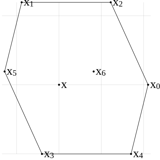
(a) Rauzy points in the B-layers at the levels up to $1$.

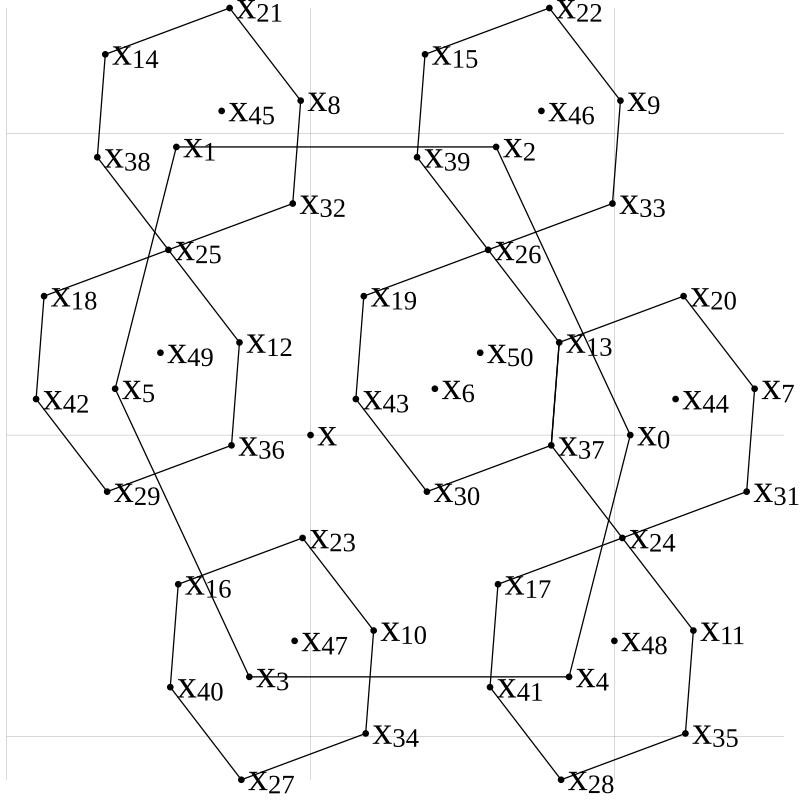
(b) Rauzy points in the B-layer at the levels up to $2$.

Figure 6. Rauzy points generated by sets $W_{i}$.

Before we procede to the proof, let us visualize how Theorem 2 contruct Rauzy fractal and its boundary. To help understanding, we will use the terminologies that we defined in previous sections here in similar ways. The set $W_{i}$ is the $i$-layer of type B, the point $\mathbf{x}+\sum\mathbf{s}_{i}^{(k)}$ is the child of $\mathbf{x}$, and the hexagon bounded by the outer six children is the cell of $\mathbf{x}$. Figure 6(a) and 6(b) shows the points in the $1$-layer and $2$-layer respectively. Unlike to the layers of type A, each point in the $(i-1)$-layer of type A is the parent to the seven children points in the $i$-layer of type A.

The morphic pattern in Equations (74) - (82) is obtained by the following observation. The tribonacci word $[\mathbf{a}_{6}]$ is obtained from concatenating copies of $[\mathbf{a}_{3}]=[0102010]$ with trimmings at the right end:

(84) $$[\mathbf{a}_{6}]=[\underbrace{0102010}_{0\textrm{ trim}}]\Big{|}[\underbrace{010201}_{1\textrm{ trim}}]\Big{|}[\underbrace{0102010}_{0\textrm{ trim}}]\Big{|}[\underbrace{0102}_{\underline{3}\textrm{ trims}}]\Big{|}[\underbrace{0102010}_{0\textrm{ trim}}]\Big{|}[\underbrace{010201}_{1\textrm{ trim}}]\Big{|}[\underbrace{0102010}_{0\textrm{ trim}}]$$

The numbers of trims follows the pattern of letters in $[\mathbf{a}_{3}]$, except for the case of letter $2$: we trim $3$ letters instead of $2$. That means, we follow the sequence $0102010$ from left to right and trim the last $0$, $1$, or $3$ characters from $[\mathbf{a}_{3}]$ to obtain substrings and concatenating them. The tribonacci $[\mathbf{a}_{9}]$ satisfies the same pattern. Each substring in $[\mathbf{a}_{6}]$ separated by $|$ in Equation (84) become a new unit for the next trimming. For example, the first substring of $[\mathbf{a}_{9}]$ is obtained by trimming the last $[0102010]$ from $[\mathbf{a}_{6}]$ (not $[0]$).

The exception at the letter $2$ is essential to obtain the Rauzy fractal. Because of the exception at $2$, we will call this pattern as pseudo self-replicating. Interestingly, removing this exception seems to give discrete tiling of $\mathbb{R}^{2}$ with a compact domain. Tilings obtained by fully self-replicating pattern will be explored in the next section.

Theorem 2 implies that we can produce Rauzy points by the simple pattern from the sequence $0102010$ using the three vectors $\mathbf{u}_{0}$, $\mathbf{u}_{1}$, $\mathbf{u}_{2}$. The construction B also gives the boundary of Rauzy fractal. In fact, it gives the same figures as in Figure 4. We take only the boundary points at each B-layers and produce children points at the next layer. The only difference between the A-layers and the B-layers is that the B-layers contains children that are lie interior to the cells of their parent. For example the point $\mathbf{x}_{6}$ in Figure 6(a) lies at the level $1$ for the A-layer, but it appears at the level $0$ for the B-layer.

The upshot for using the construction B is that the ingredients to produce Rauzy fractal and its boundary are essentially the three vectors $\mathbf{u}_{0},\mathbf{u}_{1},\mathbf{u}_{2}$ and the self-replicating sequence $0102010$. Although we need an exception at the letter $2$ to draw the Rauzy fractal, it is much simpler than having six rules in Equations (31) - (36). Moreover, the construction A requires to prepare the Rauzy points $\mathbf{b}_{i}^{(j)}$, where as the construction B requires none.

Now let us prove Theorem 2. We will show that the following holds for all $i\geq 0$:

(85) $$V_{i}\subset W_{i}\subset V_{i+1}^{(0)}.$$

In particular, we will show that the following equalities hold for all $i\geq 0$:

(86) $$\mathbf{s}_{i}^{(0)}=\mathbf{s}_{i}^{(2)}=\mathbf{s}_{i}^{(4)}=\mathbf{s}_{i}^{(6)} =\mathbf{b}_{i}^{(0)},$$

(87) $$\mathbf{s}_{i}^{(1)}=\mathbf{s}_{i}^{(5)} =\mathbf{b}_{i}^{(1)}-\mathbf{b}_{i}^{(0)},$$

(88) $$\mathbf{s}_{i}^{(3)} =\mathbf{b}_{i}^{(2)}-\mathbf{b}_{i}^{(0)}-\mathbf{b}_{i}^{(1)}.$$

From Equations (74) - (75), we have

(89) $$\mathbf{s}_{0}^{(0)}=\mathbf{s}_{0}^{(2)}=\mathbf{s}_{0}^{(4)}=\mathbf{s}_{0}^{(6)} =\mathbf{u}_{0} =\mathbf{b}_{0}^{(0)},$$

(90) $$\mathbf{s}_{0}^{(1)}=\mathbf{s}_{0}^{(5)} =\mathbf{u}_{1} =\mathbf{b}_{0}^{(1)}-\mathbf{b}_{0}^{(0)},$$

(91) $$\mathbf{s}_{0}^{(3)} =\mathbf{u}_{2} =\mathbf{b}_{0}^{(2)}-\mathbf{b}_{0}^{(0)}-\mathbf{b}_{0}^{(1)}.$$

Suppose that Equations (86) - (88) hold for all $i=k$. Then from Equations (76) - (82), we have

$$\mathbf{s}_{k+1}^{(0)}=\mathbf{s}_{k+1}^{(2)}=\mathbf{s}_{k+1}^{(4)}+\mathbf{s}_{k+1}^{(6)} =\mathbf{b}_{k}^{(0)}+\mathbf{b}_{k}^{(1)}+\mathbf{b}_{k}^{(2)} =\mathbf{b}_{k+1}^{(0)},$$

$$\mathbf{s}_{k+1}^{(1)}=\mathbf{s}_{k+1}^{(5)} =\mathbf{b}_{k}^{(1)}+\mathbf{b}_{k}^{(2)} =\mathbf{b}_{k+1}^{(0)}-\mathbf{b}_{k+1}^{(0)},$$

(92) $$\mathbf{s}_{k+1}^{(3)} =\mathbf{b}_{k}^{(2)} =\mathbf{b}_{k+1}^{(2)}-\mathbf{b}_{k+1}^{(0)}-\mathbf{b}_{k+1}^{(1)}$$

Therefore, we prove Equations (86) - (88). As a consequence, we have

(93) $$\mathbf{s}_{i}^{(0)} =\mathbf{b}_{i}^{(0)},$$

(94) $$\mathbf{s}_{i}^{(0)}+\mathbf{s}_{i}^{(1)} =\mathbf{b}_{i}^{(1)},$$

(95) $$\mathbf{s}_{i}^{(0)}+\mathbf{s}_{i}^{(1)}+\mathbf{s}_{i}^{(2)} =\mathbf{b}_{i}^{(0)}+\mathbf{b}_{i}^{(1)},$$

(96) $$\mathbf{s}_{i}^{(0)}+\mathbf{s}_{i}^{(1)}+\mathbf{s}_{i}^{(2)}+\mathbf{s}_{i}^{(3)} =\mathbf{b}_{i}^{(2)},$$

(97) $$\mathbf{s}_{i}^{(0)}+\mathbf{s}_{i}^{(1)}+\mathbf{s}_{i}^{(2)}+\mathbf{s}_{i}^{(3)}+\mathbf{s}_{i}^{(4)} =\mathbf{b}_{i}^{(0)}+\mathbf{b}_{i}^{(2)},$$

(98) $$\mathbf{s}_{i}^{(0)}+\mathbf{s}_{i}^{(1)}+\mathbf{s}_{i}^{(2)}+\mathbf{s}_{i}^{(3)}+\mathbf{s}_{i}^{(4)}+\mathbf{s}_{i}^{(5)} =\mathbf{b}_{i}^{(1)}+\mathbf{b}_{i}^{(2)},$$

(99) $$\mathbf{s}_{i}^{(0)}+\mathbf{s}_{i}^{(1)}+\mathbf{s}_{i}^{(2)}+\mathbf{s}_{i}^{(3)}+\mathbf{s}_{i}^{(4)}+\mathbf{s}_{i}^{(5)}+\mathbf{s}_{i}^{(6)} =\mathbf{b}_{i}^{(0)}+\mathbf{b}_{i}^{(1)}+\mathbf{b}_{i}^{(2)}=\mathbf{b}_{i+1}^{(0)}.$$

This proves Equation (85) and thus Theorem 2.

5. Self-replicating words and discrete tilings

Let $[\mathbf{w}]=[w_{0}\cdots w_{l}]$ be a word on $d$-letters. Let us denote $[\mathbf{w}_{0}]=[\mathbf{w}]$ and for $0\leq i\leq l$,

(100) $$[\mathbf{w}_{0}^{(i)}]=[w_{i}].$$

For $n\geq 0$, the $n$-th replicate of $[\mathbf{w}]$, denoted by $[\mathbf{w}_{n}]$, is the word defined by

(101) $$[\mathbf{w}_{n}]=[\mathbf{w}_{n}^{(0)}]\cdots[\mathbf{w}_{n}^{(l)}],$$

where for $0\leq i\leq l$,

(102) $$[\mathbf{w}_{n}^{(i)}]=[\mathbf{w}_{n-1}^{(0)}]\cdots[\mathbf{w}_{n-1}^{(l-w_{i})}].$$

Definition 3.

Let $\mathbf{v}_{n}$ be the word vector for $\mathbf{w}_{n}$. A word $\mathbf{w}$ is called self-replicating if the limit $\mathbf{v}_{\infty}=\displaystyle\lim\mathbf{v}_{n}/\|\mathbf{v}_{n}\|$ exists.

We will define the domains for self-replicating words as follows, in a similar way to Pisot domains, but using the ideas from the construction B. Let $P$ the hyperplane orthogonal to $\mathbf{v}_{\infty}$. Let $\mathbf{r}_{0},\cdots,\mathbf{r}_{d-2}$ be the orthonormal basis on $P$ obtained by Gram–Schmidt process on $\mathbf{v}_{\infty},\mathbf{e}_{0},\cdots,\mathbf{e}_{d-2}$. Let $\pi:\mathbb{R}^{d}\to P$ be the orthogonal projection, and $\mathbf{u}_{i}$, $i=0,\cdots,n-1$, be the $(d-1)$-dimensional vectors as follows.

(103) $$\mathbf{u}_{i}=(\pi(\mathbf{e}_{i})\circ\mathbf{r}_{0},\cdots,\pi(\mathbf{e}_{i})\circ\mathbf{r}_{n-2}).$$

We define the vectors $\mathbf{s}_{i}^{(j)}$ similar to Equations (74) - (82): for $j=0,\cdots,l$,

(104) $$\mathbf{s}_{0}^{(j)}=\mathbf{u}_{j},\quad\mathbf{s}_{i+1}^{(j)}=\sum_{k=0}^{l-a_{j}}\mathbf{s}_{i}^{(k)}\textrm{ for }i\geq 0.$$

Finally, using the same definition of the set $W_{i}$ in Equation (83), define the $(d-1)$-dimensional domain $W$ as

(105) $$W=\bigcup_{i=-1}^{\infty}W_{i}.$$

$\mathbf{w}$	$\mathbf{v}_{\infty}$
0120	(0.756, 0.521, 0.397)
0102	(0.850, 0.462, 0.251)
0201	(0.831, 0.259, 0.492)
0102010	(0.861, 0.447, 0.242)
1201	(0.381, 0.717, 0.584)
2010	(0.771, 0.359, 0.526)

Table 2. Self replicating words and their limits

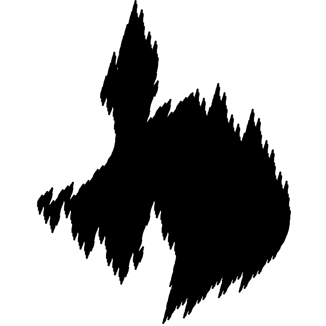
(a) 0120 “The Fish”

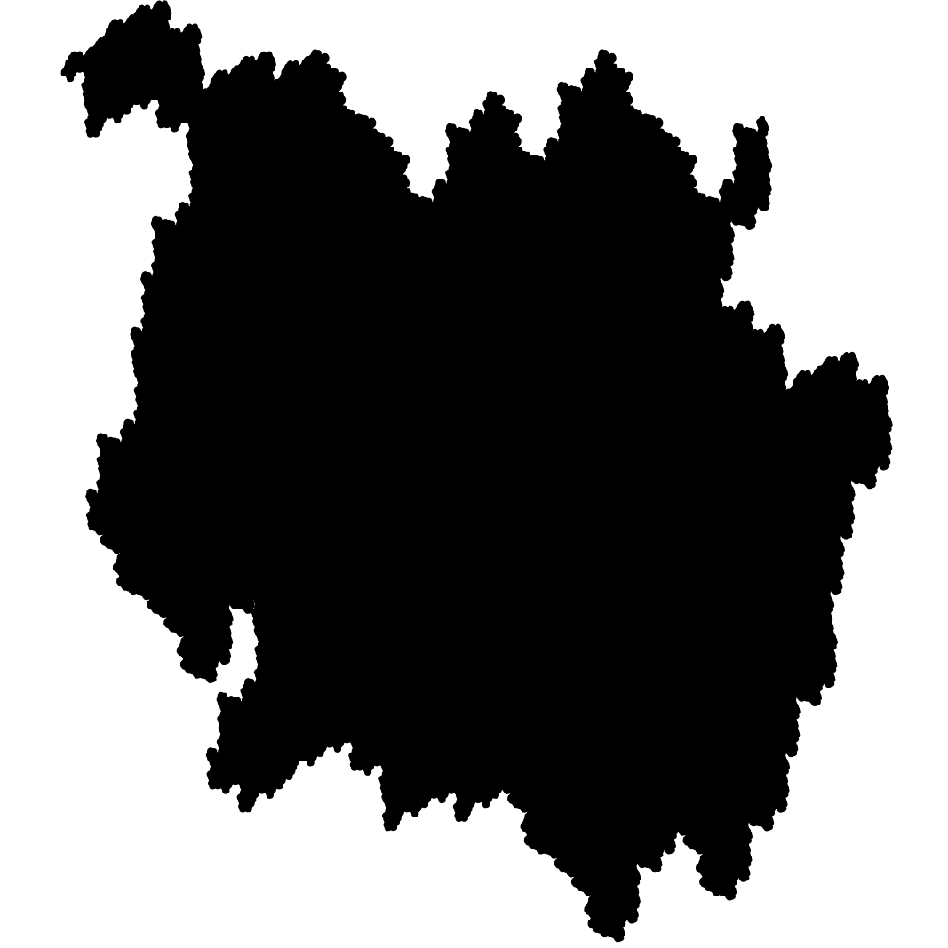
(b) 0102

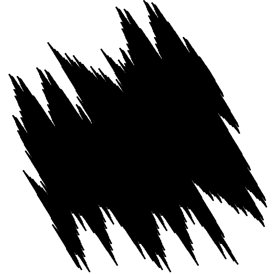
(c) 0201

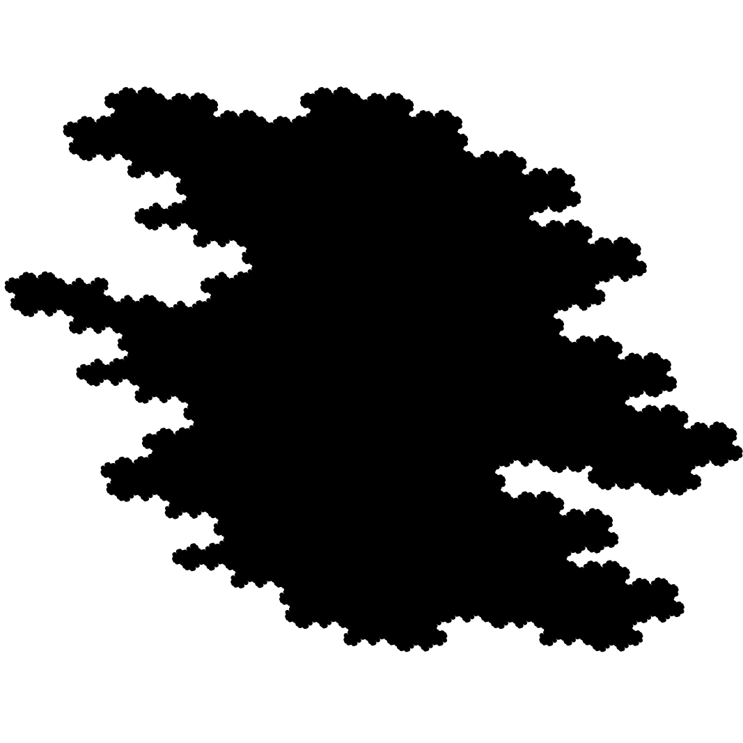
(d) 0102010

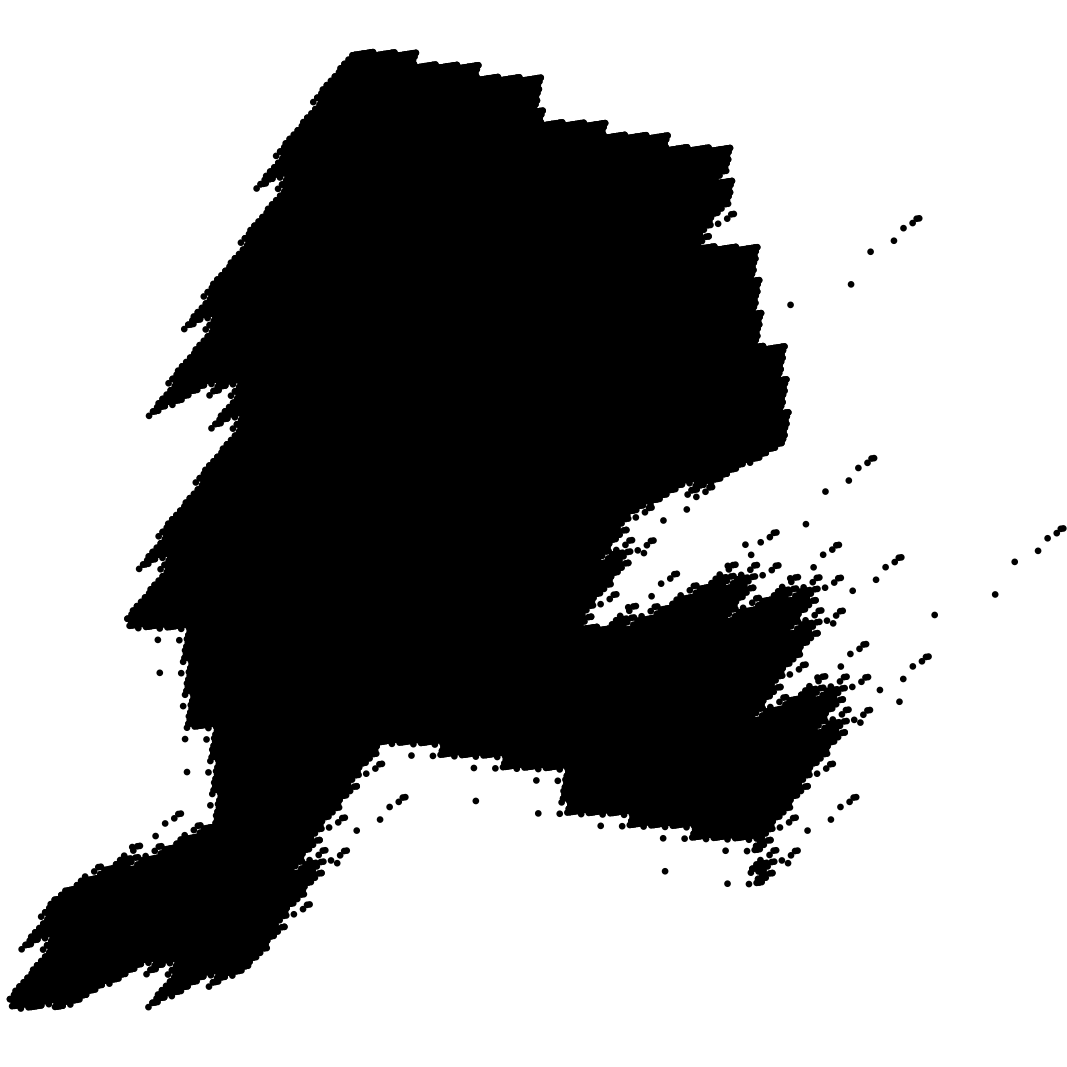
(e) 1201 “The Runner”

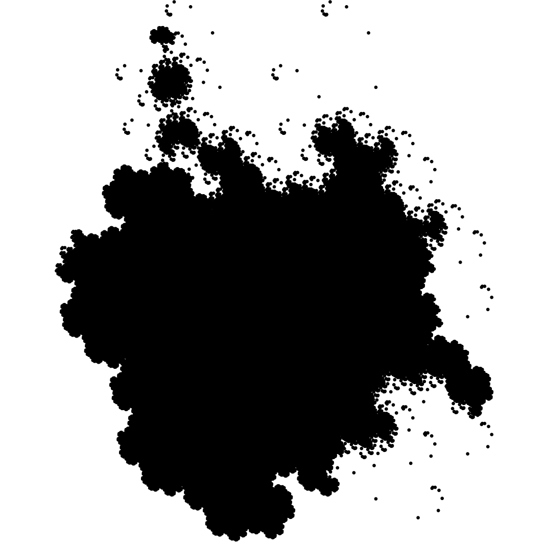
(f) 2010

Figure 7. The domains for self-replicating words

Table 2 shows some examples of self-replicating words on $3$ letters and their limits $\mathbf{v}_{\infty}$. Figure 7 shows the domain $W$ for each elf-replicating words. One can see that all domains are compact, and tiles $\mathbb{R}^{2}$ discretely. Once we have $(n-1)$-dimensional orthonormal basis $\mathbf{u}_{i}$, $i=0,\cdots,n-2$, all points in such domain can be obtained by arithmetic summations of vectors as in Equation (104).

The domains in Figure 7 tiles $\mathbb{R}^{2}$. From $\mathbf{u}_{0},\mathbf{u}_{1},\mathbf{u}_{2}$ in Equation (103), the three vectors

(106) $$\mathbf{u}_{01}=\mathbf{u}_{0}-\mathbf{u}_{1},\quad\mathbf{u}_{12}=\mathbf{u}_{1}-\mathbf{u}_{2},\quad\mathbf{u}_{02}=\mathbf{u}_{0}-\mathbf{u}_{2}$$

are the vectors that translates the domains into hexagonal tilings. For example, we can translate “The Fish” in Figure 7(a) by linear combinations of these three vectors $(1.27,-0.48),(-0.34,1.36),(0.93,0.88)$. Figure 8(a) shows the discrete tilings of Figures 7(a), 7(e). At this point, we can conjecture that the following statement is true.

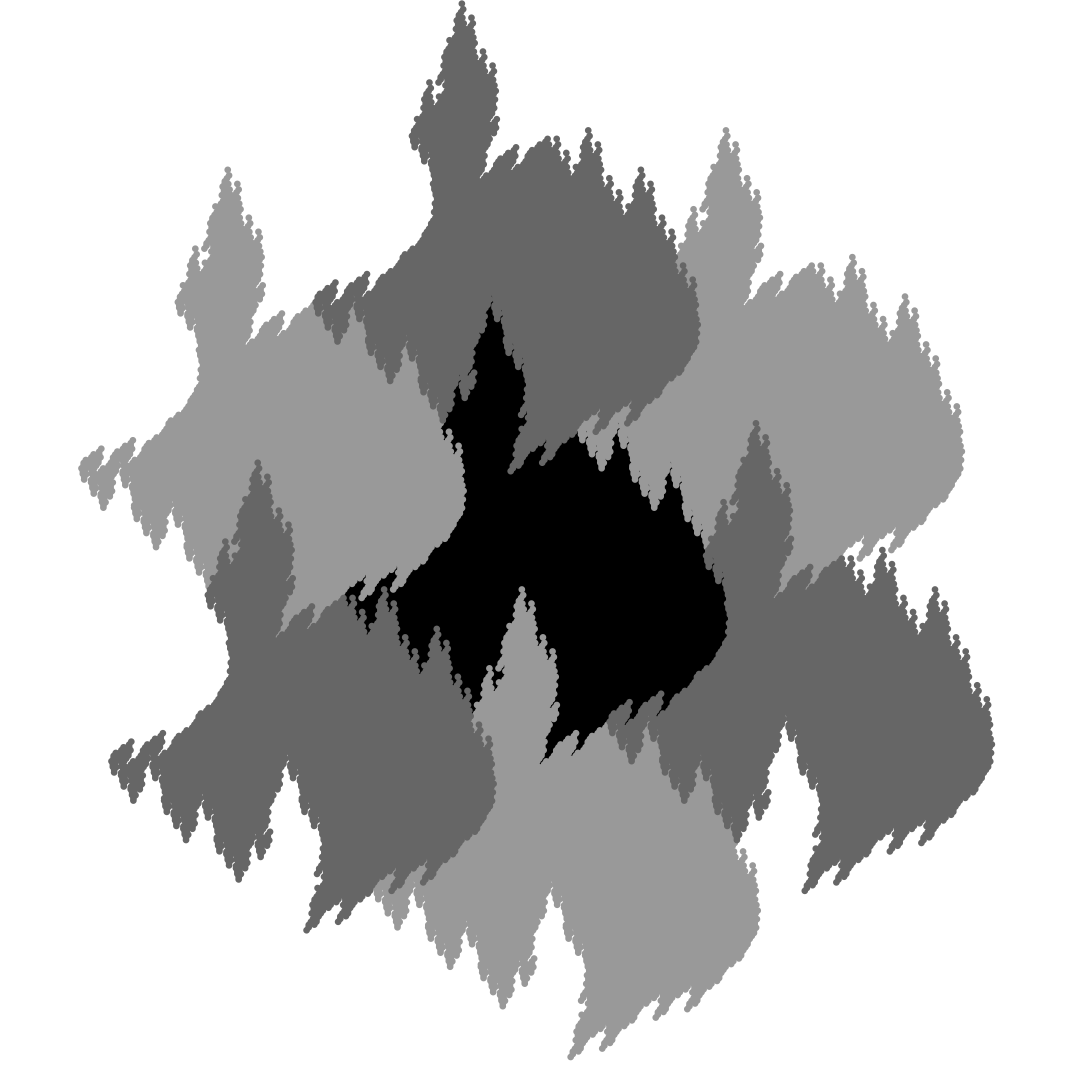
(a) The discrete tiling of “The Fish”

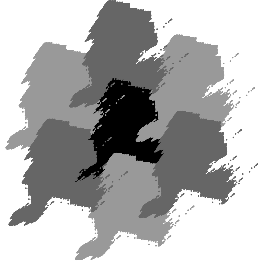
(b) The discrete tiling of “The Runner”

Figure 8. The discrete tiling of self-replicating domains,

Conjecture.

Let $[\mathbf{w}]$ be a self-replicating word on three letters. Then the domain $W$ defined in Equation (105) tiles $\mathbb{R}^{2}$ discretely in the following sense: for the vectors $\mathbf{u}_{01}$, $\mathbf{u}_{12}$, and $\mathbf{u}_{02}$ in Equation (106) and for $3$-dimensional integral vector $\mathbf{c}=(c_{01},c_{12},c_{02})$, define $W_{\mathbf{c}}=W+\sum_{i<j}c_{ij}\mathbf{u}_{ij}$. Then $W_{\mathbf{c}_{1}}\cap W_{\mathbf{c}_{2}}=\emptyset$ unless $\mathbf{c}_{1}=\mathbf{c}_{2}$ and $\mathbb{R}^{2}=\displaystyle\bigcup_{\mathbf{c}\in\mathbb{Z}^{3}}W_{\mathbf{c}}$.

6. Conclusion

The Rauzy fractal attracted mathematical interests for many years, and its characteristics have been generalized into many areas of advanced research. We studied yet another characteristics of the Rauzy fractal with an elementary view point, and showed that this characteristic can be generalized for creating another tiling scheme for the two dimensional Euclidean space. We expect that our final conjecture can be further generalized to higher dimensions.

References

[1]
S. Akiyama, M. Barge, V. Berthé, J.-Y. Lee, and A. Siegel.
On the Pisot substitution conjecture.
In Mathematics of aperiodic order, volume 309 of Progr.
Math., pages 33–72. Birkhäuser/Springer, Basel, 2015.
[2]
Pierre Arnoux and Shunji Ito.
Pisot substitutions and Rauzy fractals.
volume 8, pages 181–207. 2001.
Journées Montoises d’Informatique Théorique
(Marne-la-Vallée, 2000).
[3]
Marcy Barge.
The Pisot conjecture for -substitutions.
Ergodic Theory Dynam. Systems, 38(2):444–472, 2018.
[4]
Marcy Barge and Beverly Diamond.
Coincidence for substitutions of Pisot type.
Bull. Soc. Math. France, 130(4):619–626, 2002.
[5]
Marcy Barge and Jaroslaw Kwapisz.
Geometric theory of unimodular Pisot substitutions.
Amer. J. Math., 128(5):1219–1282, 2006.
[6]
Valerie Berthé and Anne Siegel.
Purely periodic -expansions in the Pisot non-unit case.
J. Number Theory, 127(2):153–172, 2007.
[7]
Charles Pisot.
La répartition modulo 1 et les nombres algébriques.
Ann. Scuola Norm. Super. Pisa Cl. Sci. (2), 7(3-4):205–248,
1938.
[8]
Martine Queffélec.
Substitution dynamical systems—spectral analysis, volume 1294
of Lecture Notes in Mathematics.
Springer-Verlag, Berlin, second edition, 2010.
[9]
G. Rauzy.
Nombres algébriques et substitutions.
Bull. Soc. Math. France, 110(2):147–178, 1982.
[10]
E. Arthur Robinson, Jr.
Symbolic dynamics and tilings of .
In Symbolic dynamics and its applications, volume 60 of Proc. Sympos. Appl. Math., pages 81–119. Amer. Math. Soc., Providence, RI,
2004.
[11]
Anne Siegel.
Pure discrete spectrum dynamical system and periodic tiling
associated with a substitution.
Ann. Inst. Fourier (Grenoble), 54(2):341–381, 2004.
[12]
V. F. Sirvent and B. Solomyak.
Pure discrete spectrum for one-dimensional substitution systems of
Pisot type.
volume 45, pages 697–710. 2002.
Dedicated to Robert V. Moody.
[13]
Boris Solomyak.
Dynamics of self-similar tilings.
Ergodic Theory Dynam. Systems, 17(3):695–738, 1997.
[14]
Toufik Zaïmi.
On the distribution of powers of a Gaussian Pisot number.
Indag. Math. (N.S.), 31(1):177–183, 2020.