Counting and Sampling Labeled Chordal Graphs in Polynomial Time

We present the first polynomial-time algorithm to exactly compute the number of labeled chordal graphs on $n$ vertices. Our algorithm solves a more general problem: given $n$ and $\omega$ as input, it computes the number of $\omega$-colorable labeled chordal graphs on $n$ vertices, using $O(n^{7})$ arithmetic operations. A standard sampling-to-counting reduction then yields a polynomial-time exact sampler that generates an $\omega$-colorable labeled chordal graph on $n$ vertices uniformly at random. Our counting algorithm improves upon the previous best result by Wormald (1985), which computes the number of labeled chordal graphs on $n$ vertices in time exponential in $n$.

An implementation of the polynomial-time counting algorithm gives the number of labeled chordal graphs on up to $30$ vertices in less than three minutes on a standard desktop computer. Previously, the number of labeled chordal graphs was only known for graphs on up to $15$ vertices.

1 Introduction

Generating random graphs from a prescribed graph family is a fundamental task for running simulations and testing conjectures. Although generating a random labeled graph on $n$ vertices is easy (just flip an unbiased coin for each potential edge), the first polynomial-time algorithm for generating an unlabeled graph uniformly at random was only given in 1987, by Wormald [37]. The algorithm of Wormald runs in polynomial time in expectation, and to the best of our knowledge, the existence of a worst-case polynomial-time sampler of random unlabeled graphs remains open.

Naturally, when we wish to sample from a specified graph family, there are many interesting families of graphs for which this problem is nontrivial, even when the graphs are labeled. For the class of labeled trees, a sampling algorithm using Prüfer sequences [28] was discovered in 1918. More recently, a fast (exact) uniform sampler was presented by Gao and Wormald for $d$-regular graphs with $d=o(\sqrt{n})$ in 2017 [12], and then for power-law graphs in 2018 [13]. A more general problem is the following: given an arbitrary degree sequence, generate a random graph with those specified degrees — this has been resolved for bipartite graphs [22, 3] as well as for general graphs when the maximum degree is not too large [17, 1]. See Greenhill [16] for a survey of random generation of graphs with degree constraints. For planar graphs, Bodirsky, Gröpl, and Kang presented a polynomial-time algorithm [7], which uses dynamic programming to exactly compute the number of labeled planar graphs on $n$ vertices and generate a planar graph uniformly at random in time $\widetilde{O}(n^{7})$. This was improved to $O(n^{2})$ expected time by Fusy [11], using a Boltzmann sampler.

Our results fall naturally within this line of work. We consider the problem of generating a labeled chordal graph on $n$ vertices uniformly at random. A graph is chordal if it has no induced cycles of length at least 4. Despite being one of the most fundamental and well-studied graph classes, prior to our work, the fastest uniform sampling algorithm for labeled chordal graphs was the exponential-time algorithm of Wormald from 1985 [36]. (To be precise, optimizing the running time of an algorithm for counting chordal graphs was not the main focus of Wormald; rather, the main goal of the paper was to determine the asymptotic number of chordal graphs with given connectivity, and the exponential-time algorithm is a corollary of these results.) Since then, various algorithmic approaches have been proposed for generating chordal graphs (e.g., [24, 33, 34, 9, 25]), but these algorithms do not come with any formal guarantees about their output distribution. In particular, [33] specifically asks for the existence of a polynomial-time algorithm to sample chordal graphs uniformly at random as an open problem. In a recent abstract, Sun and Bezáková [34] proposed a Markov chain for sampling chordal graphs, but this Markov chain comes with few mixing time guarantees.

We obtain the first polynomial (in $n$) time algorithm to exactly count the number of labeled chordal graphs on $n$ vertices, as well as the first polynomial-time uniform sampling algorithm for the class of labeled chordal graphs. Our algorithm also easily extends to counting and sampling $\omega$-colorable labeled chordal graphs. A graph $G$ is $\omega$-colorable if there exists a function $c\colon V(G)\to\{1,\ldots,\omega\}$ such that every edge $uv\in E(G)$ satisfies $c(u)\neq c(v)$.

Theorem 1.1.

There is a deterministic algorithm that given positive integers $n$ and $\omega\leq n$, computes the number of $\omega$-colorable labeled chordal graphs on $n$ vertices using $O(n^{7})$ arithmetic operations. Moreover, there is a randomized algorithm that given the same input, generates a graph uniformly at random from the set of all $\omega$-colorable labeled chordal graphs on $n$ vertices using $O(n^{7})$ arithmetic operations.

By the known equivalence between chromatic number, maximum clique size, and treewidth of chordal graphs [6], Theorem 1.1 can be reinterpreted as counting and sampling labeled chordal graphs of clique size at most $\omega$, or treewidth at most $\omega-1$. The running time bound of Theorem 1.1 is stated in terms of the number of arithmetic operations. Since there are at most $2^{n^{2}}$ labeled graphs on $n$ vertices, the arithmetic operations need to deal with $n^{2}$-bit integers. Therefore, using the $O(n\log{n})$-time algorithm for multiplying two $n$-bit integers [20] yields an $O(n^{9}\log n)$-time upper bound for our algorithm in the RAM model.

A straightforward implementation of our counting algorithm gives the number of labeled chordal graphs on up to $n=30$ vertices in less than three minutes on a standard desktop computer. Previously, the number of labeled chordal graphs was only known for graphs on up to $15$ vertices [26]. In addition, we use our implementation to compute the number of $\omega$-colorable labeled chordal graphs for $n\leq 12$ and $\omega\leq 12$. We chose to stop at $n=12$ to keep the table at a reasonable size, not because of the computation time. We present the computational results in Section 4.

1.1 A Brief Survey on Chordal Graphs

The literature on chordal graphs is so vast that it would be impossible to fully do it justice. Discussions of chordal graphs in the literature go as far back as 1958 [19]. What follows is a summary of some of the most notable problems and milestones.

Many NP-hard optimization problems (such as coloring [14] and maximum independent set [10]), as well as #P-hard counting problems (such as independent sets [27, 4]), and many others [30], are polynomial-time solvable on chordal graphs. Chordal graphs have a wide variety of applications, including phylogeny in evolutionary biology [18, 29] and Bayesian networks in machine learning [35]. When doing Gaussian elimination on a symmetric matrix, the set of matrix entries that are nonzero for at least one time-point of the elimination process corresponds to the edge set of a chordal graph. Thus the problem of finding an ordering in which to do Gaussian elimination that minimizes the number of nonzero matrix entries can be reduced to finding a chordal supergraph of a given graph with the minimum number of edges [31]. This problem, known as minimum fill-in, was shown to be NP-complete by Yannakakis [38]. Chordal graphs have a central place in graph theory [8], both through their connection to treewidth [21] and through their connection to perfect graphs [15]. From an algorithms perspective, chordal graphs can be recognized in linear time [32].

An interesting and relevant result by Bender et al. [2] is that a random $n$-vertex labeled chordal graph is a split graph with probability $1-o(1)$, i.e., the fraction of labeled chordal graphs that are not split is $o(1)$. This yields a simple approximately uniform sampler for labeled chordal graphs: simply sampling a random labeled split graph leads to an output distribution with total variation distance $o(1)$ from the uniform distribution on labeled chordal graphs. This simple sampling algorithm is unsatisfactory because it can never output a non-split chordal graph. Nevertheless, this result suggests two things: The first is that it might be possible to find a simple and efficient uniform random sampler for labeled chordal graphs. The second is that the type of chordal graphs that one usually envisions when thinking of a chordal graph (namely those with relatively small treewidth) are different from those most likely to be generated by a uniform random sampler (namely split graphs). Therefore, to generate the type of chordal graphs that one usually envisions, one should be sampling not from the set of all chordal graphs but rather from a subset, e.g., the set of all $\omega$-colorable chordal graphs. Fortunately, Theorem 1.1 provides this functionality.

1.2 Methods

Our exact counting algorithm is based on dynamic programming. While clique trees and tree decompositions are never explicitly mentioned in the description of the algorithm, the intuition behind the algorithm is based on these notions. Essentially, we generate a rooted clique tree where the dynamic-programming table encodes certain properties of the graph, including how it relates to the root node of the clique tree. A clique tree of a graph $G$ is a tree $T$ together with a function $f$ that maps each vertex of $G$ to a connected vertex subset of $T$, such that for every pair $u$,$v$ of vertices in $G$, $uv$ is an edge in $G$ if and only if $f(u)\cap f(v)\neq\emptyset$. It is well known that a graph $G$ has a clique tree if and only if it is chordal [6].

The main difficulty with this approach is that different chordal graphs have different numbers of clique trees, so if we count the total number of clique trees, this will not give us an accurate count of the number of $n$-vertex chordal graphs. Therefore, the key idea behind our algorithm is to assign to each labeled chordal graph a unique “canonical” clique tree and to only count these canonical clique trees. The information stored in the dynamic-programming table is sufficient to ensure that every clique tree that we do count is the canonical tree of some chordal graph, and that the canonical clique tree of every chordal graph is counted. As it turns out, the best way to phrase our algorithm is not in terms of clique trees at all, but rather in terms of an (essentially) equivalent notion that we call an “evaporation sequence.” An evaporation sequence is closely related to the standard notion of a perfect elimination ordering (PEO) of a chordal graph. A simplicial vertex is a vertex whose neighborhood is a clique, and a PEO is an ordering of the vertices such that each is simplicial in the current induced subgraph, if we delete the vertices in that order (see Section 3.1 for more details). An evaporation sequence is a type of “canonical” PEO: at each step, we remove all simplicial vertices from the current subgraph, rather than making an arbitrary choice of a single simplicial vertex. We say that all of the simplicial vertices evaporate at time $1$. Next, all of the vertices that become simplicial once the first set of simplicial vertices has been removed are said to evaporate at time $2$, and so on. It is easy to see that every labeled chordal graph has a unique evaporation sequence, and that this sequence does not depend on the labeling of the vertices.

Therefore, the number of chordal graphs on $n$ vertices is the sum over all evaporation sequences of the number of labeled chordal graphs with that evaporation sequence. While different evaporation sequences correspond to different numbers of chordal graphs, because this number is independent of the labels, we can simply guess the number $x$ of vertices that evaporate at any given time, and then without loss of generality assign the labels $1,\ldots,x$ to those vertices.

In our dynamic-programming algorithm, the recursive subproblems deal with counting rooted clique trees. In this context, the root of a clique tree is the set of vertices that evaporate last. Just as we would like to “force” a set of nodes to be in the root of the tree, we will sometimes want to force a set of nodes to evaporate last. This is done using what we call an exception set, i.e., a set of vertices that do not evaporate even if they are simplicial.

The random sampling algorithm in Theorem 1.1 follows from our counting algorithm using the standard sampling-to-counting reduction of [23].

1.3 Overview of the Paper

Our dynamic-programming algorithm, including the associated recurrences, is presented in Section 3. The proof of correctness of the algorithm can be found in Section 3.4 (here we reduce to counting connected chordal graphs) and Section 5 (here we establish the recurrences). In Section 6, we describe the details of how to obtain the random sampling algorithm using the counting algorithm.

2 Preliminaries

Our algorithm counts vertex-labeled chordal graphs. For simplicity of notation, we assume the vertex set of each graph is a subset of $\mathbb{N}=\{1,2,3,\ldots\}$, which allows the labels to also serve as the names of the vertices. For example, we will speak of the vertex $5\in V(G)$ rather than a vertex $v$ with label 5.

Definition 2.1.

A labeled graph is a pair $G=(V,E)$, where the vertex set $V$ is a finite subset of $\mathbb{N}$ and the edge set $E$ is a set of two-element subsets of $V$.

Henceforth, we implicitly assume all graphs that we consider are labeled graphs. For nonnegative integers $n$, we use the notation $[n]\coloneqq\{1,2,\ldots,n\}$. Intervals of integers will often appear in our algorithm as the vertex set of a graph or subgraph, so we also define

$$[a,b]\coloneqq\{a,a+1,\ldots,b\}$$

for nonnegative integers $a,b$. If $b<a$, then $[a,b]=\emptyset$.

Definition 2.2.

Let $A=\{a_{1},\ldots,a_{r}\}$ and $B=\{b_{1},\ldots,b_{r}\}$ be finite subsets of $\mathbb{N}$ such that $|A|=|B|$, where the elements $a_{i}$ and $b_{i}$ are listed in increasing order. We define $\phi(A,B)\colon A\to B$ as the bijection that maps $a_{i}$ to $b_{i}$ for all $i\in[r]$.

Definition 2.3.

Let $G_{1}$, $G_{2}$ be two graphs, and suppose $C\coloneqq V(G_{1})\cap V(G_{2})$ is a clique in both $G_{1}$ and $G_{2}$. When we say we glue $G_{1}$ and $G_{2}$ together at $C$ to obtain $G$, this indicates that $G$ is the union of $G_{1}$ and $G_{2}$: the vertex set is $V(G)=V(G_{1})\cup V(G_{2})$, and the edge set is $E(G)=E(G_{1})\cup E(G_{2})$.

For a graph $G$ and a vertex subset $S\subseteq V(G)$, $G[S]$ denotes the induced subgraph on the vertices of $S$. For a vertex $v\in V(G)$, we denote the neighborhood of $v$ in $G$ by $N_{G}(v)$, or by $N(v)$ if the graph is clear from the context. For $S\subseteq V(G)$, the open neighborhood of $S$ is denoted by

$$N_{G}(S)\coloneqq\{v\in V(G)\setminus S:uv\in E(G)\text{ for some $u\in S$}\}$$

and the closed neighborhood of $S$ is denoted by $N_{G}[S]\coloneqq S\cup N_{G}(S)$, or simply $N(S)$ and $N[S]$, respectively. For $S,T\subseteq V(G)$, we say $S$ sees all of $T$ if $T\subseteq N(S)$.

3 Counting labeled chordal graphs

3.1 The evaporation sequence

Definition 3.1.

A vertex $v$ in a graph $G$ is simplicial if $N(v)$ forms a clique.

A perfect elimination ordering of a graph $G$ is an ordering $v_{1},\ldots,v_{n}$ of the vertices of $G$ such that for all $i\in[n]$, $v_{i}$ is simplicial in the subgraph induced by the vertices $v_{i},\ldots,v_{n}$. It is well known that a graph is chordal if and only if it has a perfect elimination ordering [6]. For our counting algorithm, we define the notion of the evaporation sequence of a chordal graph, which can be viewed as a canonical version of the perfect elimination ordering. In the evaporation sequence, rather than making an arbitrary choice for which of the simplicial vertices in $G$ will go first in the ordering, we place the set of all simplicial vertices as the first item in the sequence. As an example, if $G$ is a tree, then the set of all simplicial vertices would be exactly the leaves of $G$.

To build the evaporation sequence, we use the fact that given a chordal graph $G$, if we repeatedly remove all simplicial vertices, then eventually no vertices remain. By observing at which time step each vertex is deleted, we obtain a partition of $V(G)$, which allows us to classify and understand the structure of $G$. In our algorithm, it will also be useful to set aside a set of exceptional vertices which are never deleted, even if they are simplical.

To formalize this, suppose we are given a chordal graph $G$ and a vertex subset $X\subseteq V(G)$. We define the evaporation sequence of $G$ with exception set $X$ as follows: If $X=V(G)$, then the evaporation sequence of $G$ is the empty sequence. If $X\subsetneq V(G)$, then let $\widetilde{L}_{1}$ be the set of all simplicial vertices in $G$, and let $L_{1}=\widetilde{L}_{1}\setminus X$. Suppose $L_{2},\ldots,L_{t}$ is the evaporation sequence of $G\setminus L_{1}$ (with exception set $X$). Then $L_{1},L_{2},\ldots,L_{t}$ is the evaporation sequence of $G$.

For this definition to make sense, there is one caveat: we must choose $X$ so that all vertices outside of $X$ eventually evaporate. For example, $X=\emptyset$ is always a valid choice since every chordal graph contains a simplicial vertex [6]. Without this assumption, we could potentially reach a point where $X\subsetneq V(G)$ but $X$ contains all of the simplicial vertices of $G$, in which case the evaporation sequence would not be well-defined (we never reach the base case $X=V(G)$). In our algorithm, we will always choose a valid $X$ such that all other vertices eventually evaporate.

If the evaporation sequence $L_{1},L_{2},\ldots,L_{t}$ of $G$ has length $t$, then we say $G$ evaporates at time $t$ with exception set $X$, and $t$ is called the evaporation time. We define $L_{G}(X)\coloneqq L_{t}$ to be the last set in the evaporation sequence of $G$, and we let $L_{G}(X)=\emptyset$ if the sequence is empty. Similarly, we define the evaporation time of a vertex subset: Suppose $G$ has evaporation sequence $L_{1},L_{2},\ldots,L_{t}$ with exception set $X$, and suppose $S\subseteq V(G)\setminus X$ is a nonempty vertex subset. Let $t_{S}$ be the largest index $i$ such that $L_{i}\cap S\neq\emptyset$. We say $S$ evaporates at time $t_{S}$ in $G$ with exception set $X$.

3.2 Setup for the counting algorithm

Given positive integers $n$ and $\omega$, we wish to count the number of $\omega$-colorable chordal graphs on $n$ vertices. This can easily be reduced to the problem of counting connected $\omega$-colorable chordal graphs on at most $n$ vertices (see Lemma 3.13 in Section 3.4). Therefore, our main focus is to describe the following algorithm:

Theorem 3.2.

There is an algorithm that given $n\in\mathbb{N}$, computes the number of $\omega$-colorable labeled connected chordal graphs $G$ with vertex set $[n]$ using $O(n^{7})$ arithmetic operations.

We first give an overview of this algorithm and describe the various dynamic-programming tables (Definition 3.3). Next, we describe the recurrences in detail in Section 3.3. In Section 3.4, we show that the counting portion of Theorem 1.1 (counting chordal graphs) follows from Theorem 3.2 (counting connected chordal graphs). In Section 5, we prove correctness of the recurrences and complete the proof of Theorem 3.2.

Algorithm overview. To count $\omega$-colorable connected chordal graphs $G$, we classify these graphs based on the behavior of their evaporation sequence. We make use of several counter functions (these are our dynamic-programming tables), each of which keeps track of the number of chordal graphs in a particular subclass. The arguments of the counter functions tell us the number of vertices in the graph, the evaporation time, the size of the exception set $X$, the size of the last set of simplicial vertices $L_{G}(X)$, etc. Initially, we consider all possibilities for the evaporation time of $G$ with exception set $X=\emptyset$. Then, using several of our recursive formulas, we reduce the number of vertices by dividing up the graph into smaller subgraphs and counting the number of possibilities for each subgraph. As we do so, the exception set $X$ increases in size. When we consider these various subgraphs, we also make sure that in each subgraph, the maximum clique size is at most $\omega$. In the end, the algorithm understands the possibilities for the entire graph, including the cliques that make up the very first set in its evaporation sequence.

The purpose of the exception set is to allow us to restrict to smaller subgraphs without distorting the evaporation behavior of the graph. For example, suppose we wish to count the number of connected chordal graphs on $n$ vertices that evaporate at time $t$, such that the vertices $1,2,\ldots,l$ make up the last set to evaporate, i.e., $L_{G}(\emptyset)=[l]$. Let $L=[l]$. One subproblem of interest would be to count the number of possibilities for the first connected component of $G\setminus L$. Formally, we count the number of possibilities for $G^{\prime}\coloneqq G[L\cup C]$, where $C$ is the connected component of $G\setminus L$ that contains the vertex $l+1$. For each possible number of vertices in $G^{\prime}$, we make a recursive call to count the number of possible subgraphs $G^{\prime}$ of that size. However, if we were to restrict to $G^{\prime}$ with a still-empty exception set, then the evaporation time of $G^{\prime}$ alone could be much less than the evaporation time of $V(G^{\prime})$ in $G$. Indeed, there may be vertices in $G\setminus G^{\prime}$ adjacent to $L$ that prevent $L$ from evaporating before time $t$, so when we restrict to the subgraph $G^{\prime}$, $L$ would now evaporate too soon. This would cause a cascading effect, causing vertices near $L$ to evaporate as well, and changing the entire evaporation sequence of $G^{\prime}$. To resolve this, we add the vertices of $L$ to the exception set to preserve the evaporation behavior of $G^{\prime}$.

The list of counter functions is given in Definition 3.3; see Fig. 1 for an illustration. As shown below, the number of $\omega$-colorable connected chordal graphs on $n$ vertices is the sum of various calls to the fourth function $\tilde{g}_{1}$, since $\tilde{g}_{1}(t,0,n)$ is the number of $\omega$-colorable connected chordal graphs on $n$ vertices that evaporate at time $t$ with empty exception set. To remember the names of these counter functions, one can think of them as follows: The $g$-functions keep track of the size of the exception set $X$, but these do not have information about the size of $L_{G}(X)$. The $f$-functions have an additional argument $l$, which is the size of $L_{G}(X)$. As a mnemonic, one can say that $g$ stands for “glued” and $f$ stands for “free.” In the $g$-functions, $X$ is the “root,” and all of the vertices of $X$ are glued, in the sense that they cannot evaporate. In the $f$-functions, $X\cup L_{G}(X)$ is the “root,” and some of the vertices in the root are free, since the vertices in $L_{G}(X)$ are allowed to evaporate.

Definition 3.3.

The following functions count particular subclasses of chordal graphs. Unless stated otherwise, the arguments $t,x,l,k,z$ are nonnegative integers.

1. $g(t,x,k,z)$ is the number of $\omega$-colorable connected chordal graphs $G$ with vertex set $[x+k]$ that evaporate in time at most $t$ with exception set $X=[x]$, where $X$ is a clique, with the following property: every connected component of $G\setminus X$ (if any) has at least one neighbor in $X\setminus[z]$. Domain: $t\geq 0$, $x\geq 1$, $z<x$.

2. $\tilde{g}(t,x,k,z)$ is the same as $g(t,x,k,z)$, except every connected component of $G\setminus X$ (if any) evaporates at time exactly $t$ in $G$. Note: A graph with $V(G)=X$ would be counted because in that case, $\tilde{g}$ is the same as $g$. Domain: $t\geq 1$, $x\geq 1$, $z<x$.

3. $\tilde{g}_{p}(t,x,k,z)$ is the same as $\tilde{g}(t,x,k,z)$, except no connected component of $G\setminus X$ sees all of $X$. Domain: $t\geq 1$, $x\geq 1$, $z<x$.

4. $\tilde{g}_{1}(t,x,k)$ and $\tilde{g}_{\geq 2}(t,x,k)$ are the same as $\tilde{g}(t,x,k,z)$, except every connected component of $G\setminus X$ sees all of $X$ (hence we no longer require every component of $G\setminus X$ to have a neighbor in $X\setminus[z]$), and furthermore, for $\tilde{g}_{1}$ we require that $G\setminus X$ has exactly one connected component, and for $\tilde{g}_{\geq 2}$ we require that $G\setminus X$ has at least two components. Domain for $\tilde{g}_{1}$: $t\geq 1$, $x\geq 0$. Domain for $\tilde{g}_{\geq 2}$: $t\geq 1$, $x\geq 1$.

5. $f(t,x,l,k)$ is the number of $\omega$-colorable connected chordal graphs $G$ with vertex set $[x+l+k]$ that evaporate at time exactly $t$ with exception set $X=[x]$, such that $G\setminus X$ is connected, $L_{G}(X)=[x+1,x+l]$, and $X\cup L_{G}(X)$ is a clique. Domain: $t\geq 1$, $x\geq 0$, $l\geq 1$.

6. $\tilde{f}(t,x,l,k)$ is the same as $f(t,x,l,k)$, except every connected component of $G\setminus(X\cup L_{G}(X))$ evaporates at time exactly $t-1$ in $G$, and there exists at least one such component, i.e., $X\cup L_{G}(X)\subsetneq V(G)$. Domain: $t\geq 2$, $x\geq 0$, $l\geq 1$.

7. $\tilde{f}_{p}(t,x,l,k)$ is the same as $\tilde{f}(t,x,l,k)$, except no connected component of $G\setminus(X\cup L_{G}(X))$ sees all of $X\cup L_{G}(X)$. Domain: $t\geq 2$, $x\geq 0$, $l\geq 1$.

8. $\tilde{f}_{p}(t,x,l,k,z)$ is the same as $\tilde{f}_{p}(t,x,l,k)$, except every connected component of $G\setminus(X\cup L_{G}(X))$ has at least one neighbor in $(X\cup L_{G}(X))\setminus[z]$. Domain: $t\geq 2$, $x\geq 0$, $l\geq 1$, $z\leq x$.

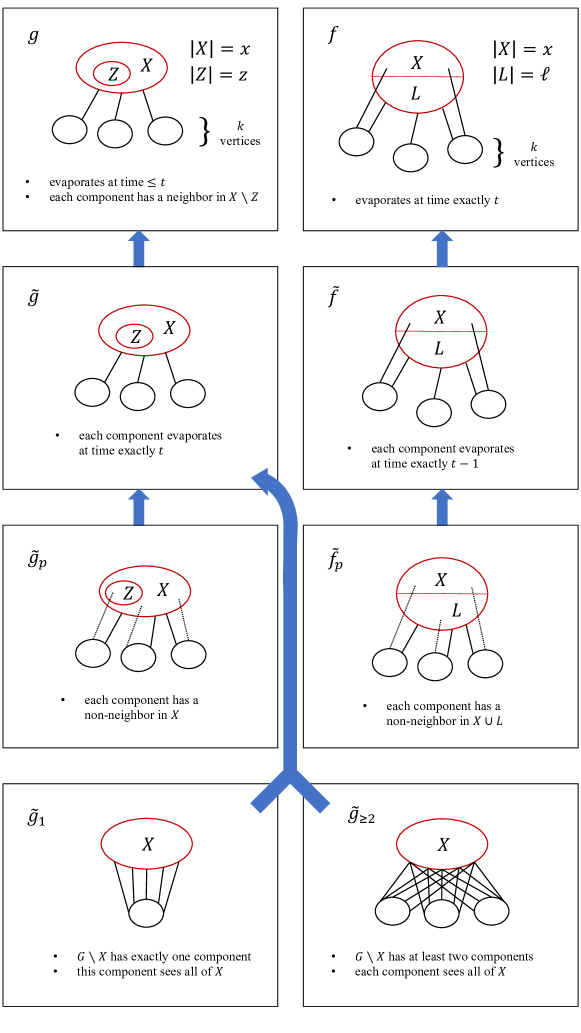
Figure 1: The counter functions. Here $L=L_{G}(X)$ and $Z=[z]$. An arrow from one function to another, say from $\tilde{g}$ to $g$, indicates that the definition of $\tilde{g}$ is the same as that of $g$, except where indicated otherwise. The drawing of $\tilde{f}_{p}$ represents $\tilde{f}_{p}(t,x,l,k)$. The function $\tilde{f}_{p}(t,x,l,k,z)$ is similar but also keeps track of the argument $z$.

3.3 Recurrences for the counting algorithm

We implicitly assume all graphs in this section are connected and $\omega$-colorable. For $k\in\mathbb{N}$, let $c(k)$ denote the number of $\omega$-colorable connected chordal graphs with vertex set $[k]$. To compute $c(n)$, we first consider all possibilities for the evaporation time. Initially, the exception set is empty. We observe that $\tilde{g}_{1}(t,0,n)$ is the number of (connected, $\omega$-colorable) chordal graphs with vertex set $[n]$ that evaporate at time exactly $t$ with empty exception set. Therefore,

$$c(n)=\sum_{t=1}^{n}\tilde{g}_{1}(t,0,n).$$

We compute the necessary values of $\tilde{g}_{1}$ by evaluating the following recurrences top-down using memoization. We take this approach rather than bottom-up dynamic programming to simplify the description slightly, since by memoizing we do not need to specify in what order the entries of the various dynamic-programming tables are computed. We simply compute each value of the counter functions as needed. For the following recurrences, let $X=[x]$ according to the current value of the argument $x$, and let $L=L_{G}(X)$.

To compute $\tilde{g}_{1}(t,0,n)$, the number of chordal graphs that evaporate at time exactly $t$, we consider all possibilities for the size $l$ of $L$. Once the size $l$ is given, there are $\binom{n}{l}$ possibilities for the label set of $L$. Recall that $f$ counts the number of chordal graphs where $L$ is fixed and evaporates at time $t$, and $G\setminus X$ is connected. Formally, we have the following recurrence — the first time this is used, the arguments are $t$, $x=0$ and $k=n$.

Lemma 3.4.

For $\tilde{g}_{1}$, we have

$$\tilde{g}_{1}(t,x,k)=\sum_{l=1}^{k}\binom{k}{l}f(t,x,l,k-l).$$

The proof of Lemma 3.4, along with the proofs of all of the other recurrences, can be found in Section 5.3. We proceed in this order, first presenting the recurrences and later presenting their proofs, to first give the reader the context of the algorithm. For now, to see the intuition behind Lemma 3.4, recall that in the definition of $f(t,x,l,k)$ we require a specific label set for $L_{G}(X)$, namely $[x+1,x+l]$. If we were to replace that requirement with $L_{G}(X)=L^{\prime}$ for any other subset $L^{\prime}$ of $[x+1,x+l+k]$ of size $l$, this would not change the value of $f(t,x,l,k)$. Therefore, in the recurrence for $\tilde{g}_{1}$, it is sufficient to compute $f(t,x,l,k-l)$ and multiply by $\binom{k}{l}$, rather than computing $\binom{k}{l}$ distinct counter functions.

For $f$, to count chordal graphs where $L$ is fixed and evaporates at time $t$, and $G\setminus X$ is connected, we consider all possibilities for the set of labels that appear in components of $G\setminus(X\cup L)$ that evaporate at time exactly $t-1$. Recall that $\tilde{f}$ counts the number of chordal graphs where $L$ is fixed and evaporates at time $t$, $G\setminus X$ is connected, and all components of $G\setminus(X\cup L)$ evaporate at time exactly $t-1$. For each possible $k^{\prime}$ (the size of this label set), $\tilde{f}$ allows us to count the number of possibilities for the subgraph $G_{1}$ consisting of $X\cup L$ and all components of $G\setminus(X\cup L)$ that evaporate at time exactly $t-1$, and $g$ allows us to count the number of possibilities for the subgraph $G_{2}$ consisting of $X\cup L$ and all other components.

Lemma 3.5.

For $f$, we have

$$f(t,x,l,k)=\sum_{k^{\prime}=1}^{k}\binom{k}{k^{\prime}}\tilde{f}(t,x,l,k^{\prime})g(t-2,x+l,k-k^{\prime},x).$$

When $f$ is called for the first time in the initial steps of the algorithm, this is the first moment when $X$ becomes nonempty, since at this point we are restricting to a subgraph with fewer than $n$ vertices. When we restrict to the subgraph $G_{2}$, we want to ensure that its vertices have the same evaporation behavior as they did in $G$. In particular, we need to ensure that the vertices of $L$ do not evaporate too soon, since their presence may be essential for preventing other vertices from evaporating. For this reason, we let $X\cup L$ be the exception set for $G_{2}$. For $G_{1}$, the exception set is simply $X$ because the components that evaporate at time exactly $t-1$ are still present in $G_{1}$, preventing the vertices of $L$ from evaporating before time $t$.

For the subgraph $G_{2}$, now that all of $L$ has been pushed into the exception set, we no longer have information about the argument $l$ since the last set of simplicial vertices in $G_{2}$ evaporates further back in time. This is why we call $g$ rather than $f$ to count the possibilities for $G_{2}$. In fact, $G_{2}\setminus[x+l]$ might not even be connected, which is required by $f$. Finally, the fourth argument of $g$ indicates that every connected component of $G_{2}\setminus(X\cup L)$ has at least one neighbor in $L$. This ensures that $G\setminus X$ is connected.

For $g$, to count chordal graphs that evaporate in time at most $t$, we consider all possibilities for the set of labels that appear in connected components of $G\setminus X$ that evaporate at time exactly $t$. Recall that $\tilde{g}$ counts the number of chordal graphs where all connected components of $G\setminus X$ evaporate at time exactly $t$.

Lemma 3.6.

For $g$, we have

$$g(t,x,k,z)=\sum_{k^{\prime}=0}^{k}\binom{k}{k^{\prime}}\tilde{g}(t,x,k^{\prime},z)g(t-1,x,k-k^{\prime},z).$$

For $\tilde{g}$, to count chordal graphs where all connected components of $G\setminus X$ evaporate at time exactly $t$, we consider all possible label sets for the component $C$ of $G\setminus X$ that contains the lowest label not in $X$. The constraint $x^{\prime}\geq 1$ ensures that $G$ is connected. We also subtract all ways of selecting $x^{\prime}$ elements from $[z]$ to ensure that $N(C)$ is not entirely contained in $[z]$.

Lemma 3.7.

For $\tilde{g}$, we have

$$\tilde{g}(t,x,k,z)=\sum_{k^{\prime}=1}^{k}\sum_{x^{\prime}=1}^{x}\left(\binom{x}{x^{\prime}}-\binom{z}{x^{\prime}}\right)\binom{k-1}{k^{\prime}-1}\tilde{g}_{1}(t,x^{\prime},k^{\prime})\tilde{g}(t,x,k-k^{\prime},z).$$

We subtract 1 in the binomial coefficient $\binom{k-1}{k^{\prime}-1}$ because the label set for $C$ always contains the lowest non-$X$ label, along with $k^{\prime}-1$ other labels.

For $\tilde{f}$, we need to count chordal graphs where $L$ is fixed and evaporates at time $t$, $G\setminus X$ is connected, and all components of $G\setminus(X\cup L)$ evaporate at time exactly $t-1$. The number of such graphs in which zero components see all of $X\cup L$ is $\tilde{f}_{p}(t,x,l,k)$. Now if there is at least one all-seeing component, then we break this down into two further cases: either exactly one component sees all of $X\cup L$, or at least two components see all of $X\cup L$. Recall that $\tilde{f}_{p}$ counts the number of chordal graphs where $L$ is fixed and evaporates at time $t$, all components of $G\setminus(X\cup L)$ evaporate at time exactly $t-1$, and no component sees all of $X\cup L$. Also, recall that $\tilde{g}_{\geq 2}$ counts the number of chordal graphs where all components of $G\setminus X$ evaporate at time exactly $t$, every component sees all of $X$, and there are at least two such components. In the first (resp. second) case, $\tilde{g}_{1}$ (resp. $\tilde{g}_{\geq 2}$) corresponds to the all-seeing component(s), and $\tilde{f}_{p}$ (resp. $\tilde{g}_{p}$) corresponds to the remaining components.

Lemma 3.8.

For $\tilde{f}$, we have

$$\tilde{f}(t,x,l,k) =\tilde{f}_{p}(t,x,l,k)+\sum_{k^{\prime}=1}^{k}\binom{k}{k^{\prime}}\tilde{g}_{1}(t-1,x+l,k^{\prime})\tilde{f}_{p}(t,x,l,k-k^{\prime})$$

$$\quad+\sum_{k^{\prime}=1}^{k}\binom{k}{k^{\prime}}\tilde{g}_{\geq 2}(t-1,x+l,k^{\prime})\tilde{g}_{p}(t-1,x+l,k-k^{\prime},x).$$

The above cases are relevant because if at least two components of $G\setminus(X\cup L)$ see all of $X\cup L$, then this prevents the vertices of $L$ from evaporating before time $t$. Indeed, each vertex $u\in L$ has a neighbor in each of those two components, meaning $u$ has two non-adjacent neighbors. Otherwise, if there is at most one such component, then the neighborhoods of the remaining components of $G\setminus(X\cup L)$ must together cover $L$ to ensure that $L$ does not evaporate until time $t$. In that case, for each vertex $u\in L$ that is covered by a proper-subset neighborhood $N(C)$ of a component $C$, $u$ has a neighbor $v\in C$ as well as a neighbor $w\in(X\cup L)\setminus N(C)$, and $v$ and $w$ are non-adjacent.

The reason we require $G\setminus X$ to be connected in the definition of $f$ (rather than just requiring $G$ to be connected) can be seen from the recurrence for $\tilde{f}$. Since in the first sum over $k^{\prime}$ we only wish to consider graphs with exactly one all-seeing component, in the definition of $\tilde{g}_{1}$ we require $G\setminus X$ to be connected. The recurrence for $\tilde{g}_{1}$ depends on $f$, so this carries over into requiring $G\setminus X$ to be connected in the definition of $f$. This explains the need for the argument $z$ (for example, in $g$): as mentioned above, keeping track of $z$ lets us ensure that $G\setminus X$ is connected in all graphs counted by $f$.

For $\tilde{g}_{\geq 2}$, to count chordal graphs where all components of $G\setminus X$ evaporate at time exactly $t$, every component sees all of $X$, and there are at least two such components, we consider all possibilities for the label set of the component that contains the lowest label not in $X$. For the remaining components, there is either exactly one of them, or at least two.

Lemma 3.9.

For $\tilde{g}_{\geq 2}$, we have

$$\tilde{g}_{\geq 2}(t,x,k)=\sum_{k^{\prime}=1}^{k-1}\binom{k-1}{k^{\prime}-1}\tilde{g}_{1}(t,x,k^{\prime})\Big{(}\tilde{g}_{1}(t,x,k-k^{\prime})+\tilde{g}_{\geq 2}(t,x,k-k^{\prime})\Big{)}.$$

For $\tilde{g}_{p}$, to count chordal graphs where all components of $G\setminus X$ evaporate at time exactly $t$ and no component sees all of $X$, we proceed as we did for $\tilde{g}$, except we require $x^{\prime}<x$ rather than $x^{\prime}\leq x$.

Lemma 3.10.

For $\tilde{g}_{p}$, we have

$$\tilde{g}_{p}(t,x,k,z)=\sum_{k^{\prime}=1}^{k}\sum_{x^{\prime}=1}^{x-1}\left(\binom{x}{x^{\prime}}-\binom{z}{x^{\prime}}\right)\binom{k-1}{k^{\prime}-1}\tilde{g}_{1}(t,x^{\prime},k^{\prime})\tilde{g}_{p}(t,x,k-k^{\prime},z).$$

For $\tilde{f}_{p}$, to count chordal graphs where $L$ is fixed and evaporates at time $t$, all components of $G\setminus(X\cup L)$ evaporate at time exactly $t-1$, and no component sees all of $X\cup L$, we first declare that no component can see only into $X$ (since $G\setminus X$ is connected).

Lemma 3.11.

We have $\tilde{f}_{p}(t,x,l,k)=\tilde{f}_{p}(t,x,l,k,x)$.

The following recurrence for $\tilde{f}_{p}$ counts the number of such graphs in which every component of $G\setminus(X\cup L)$ has at least one neighbor in $(X\cup L)\setminus[z]$. On the first reading, one can skip the two “otherwise” cases in Lemma 3.12. In this lemma, we consider all possibilities for the label set of the component $C$ of $G\setminus(X\cup L)$ that contains the lowest label not in $X\cup L$. Additionally, we consider all possibilities for the size $x^{\prime}$ of $N(C)\cap X$ and the size $l^{\prime}$ of $N(C)\cap L$, and we consider all possibilities for their respective label sets. If $l^{\prime}>0$, then $N(C)$ is automatically not contained in $[z]$ since $z\leq x$, so there are $\binom{x}{x^{\prime}}$ possible label sets for $N(C)\cap X$.

The intuition behind the two “otherwise” cases is as follows. If $l^{\prime}=0$, then we must subtract $\binom{z}{x^{\prime}}$ from the number of possible label sets for $N(C)\cap X$ to ensure that $N(C)\subsetneq[z]$. If $l^{\prime}=l$, then all of the vertices of $L$ have now been pushed into the exception set, so the evaporation time of the subgraph formed from the remaining components is $t-1$. In this case, we call $\tilde{g}_{p}$ since we no longer know the size of the last set of simplicial vertices.

Lemma 3.12.

For $\tilde{f}_{p}(t,x,l,k,z)$, we have

$$\tilde{f}_{p}(t,x,l,k,z)=$$

$$\sum_{k^{\prime}=1}^{k}\sum_{\begin{subarray}{c}0\leq x^{\prime}\leq x\\ 0\leq l^{\prime}\leq l\\ 0<x^{\prime}+l^{\prime}<x+l\end{subarray}}\binom{k-1}{k^{\prime}-1}\binom{l}{l^{\prime}}\tilde{g}_{1}(t-1,x^{\prime}+l^{\prime},k^{\prime}) \boldsymbol{\cdot}\begin{cases}\binom{x}{x^{\prime}}&\text{ if $l^{\prime}>0$}\\ \binom{x}{x^{\prime}}-\binom{z}{x^{\prime}}&\text{ otherwise}\end{cases}$$

$$\boldsymbol{\cdot}\begin{cases}\tilde{f}_{p}(t,x+l^{\prime},l-l^{\prime},k-k^{\prime},z)&\text{if $l^{\prime}<l$}\\ \tilde{g}_{p}(t-1,x+l^{\prime},k-k^{\prime},z)&\text{otherwise}.\end{cases}$$

The base cases are as follows. We reach the base case for $g$ when $t=0$:

$$g(0,x,k,z)=\begin{cases}1&\text{ if $k=0$}\\ 0&\text{ if $k>0$}.\end{cases}$$

For $\tilde{g}$ and $\tilde{g}_{p}$, we have $\tilde{g}(t,x,0,z)=1$ and $\tilde{g}_{p}(t,x,0,z)=1$ when $k=0$. For, $\tilde{g}_{1}$ we observe that $\tilde{g}_{1}(t,x,k)=0$ if $t=0$ or $k=0$. Similarly, for $\tilde{g}_{\geq 2}$ we have $\tilde{g}_{\geq 2}(t,x,k)=0$ if $t=0$ or $k=0$. We reach the base case for $f$ when $x+l>\omega$, $t=1$, or $k=0$. If $x+l>\omega$, then $f(t,x,l,k)=0$. Remarkably, this is the only place where $\omega$ appears in the algorithm. If $x+l\leq\omega$, then we have

$$f(1,x,l,k)=\begin{cases}1&\text{ if $k=0$}\\ 0&\text{ otherwise}.\end{cases}$$

If $x+l\leq\omega$ and $t\geq 2$, then $f(t,x,l,0)=0$. For $\tilde{f}$, we have $\tilde{f}(t,x,l,k)=0$ if $t=1$ or $k=0$. Similarly, for $\tilde{f}_{p}$ we have $\tilde{f}_{p}[t,x,l,k,z]=0$ if $t=1$ or $k=0$. For the version of $\tilde{f}_{p}$ without the fifth argument $z$, we do not need a base case since we always immediately call $\tilde{f}_{p}$ with $z$.

The control flow formed by these recurrences is shown in Fig. 2. The algorithm terminates because either the value of $t$ or the number of vertices in the graph (i.e., $x+k$ or $x+l+k$) decreases each time we return to the same function. For the running time, this is dominated by the arithmetic operations needed to compute $\tilde{f}_{p}$. The recurrence for $\tilde{f}_{p}$ involves a triple summation, and there are five arguments, so a naive implementation uses $O(n^{8})$ arithmetic operations. However, in Section 5.4, we show that the running time can in fact be improved to $O(n^{7})$ arithmetic operations.

Figure 2: The control flow of the counting algorithm. An arrow from $f$ to $g$ indicates that the recursive formula for $f$ depends on $g$. The arrow is red (and dashed) if $t$ decreases by 1, blue (and dashed) if $t$ decreases by 2, and black if $t$ does not change. The black self-loops do not cause an infinite loop because in those recursive calls, the number of vertices decreases.

3.4 Proof of Theorem 1.1 (counting)

In this section, we prove the counting portion of Theorem 1.1 using Theorem 3.2. (See Section 6 for the proof of the sampling portion of Theorem 1.1.) In other words, we describe an algorithm to count chordal graphs, assuming we have an algorithm to count connected chordal graphs. Theorem 3.2 — counting connected chordal graphs — is proved in Section 5.

For $k\in\mathbb{N}$, let $a(k)$ denote the number of $\omega$-colorable chordal graphs with vertex set $[k]$. Recall that $c(k)$ is the number of $\omega$-colorable connected chordal graphs with vertex set $[k]$.

Lemma 3.13.

The number of $\omega$-colorable chordal graphs with vertex set $[n]$ is given by

$$a(n)=\sum_{k=1}^{n}\binom{n-1}{k-1}c(k)a(n-k)$$

for all $n\in\mathbb{N}$.

Proof.

Suppose $G$ is an $\omega$-colorable chordal graph with vertex set $[n]$. Let $G_{1}$ be the graph formed by the connected component of $G$ that contains the label 1, and let $G^{\prime}$ be the graph formed by all other connected components of $G$ (which can potentially be empty). Let $C$ be the set of labels that appear in $G_{1}$, let $k=|C|$, and let $D=[n]\setminus C$, i.e., $D$ is the set of labels that appear in $G^{\prime}$. Now relabel $G_{1}$ by applying $\phi(C,[k])$ to the labels in $C$, and relabel $G^{\prime}$ by applying $\phi(D,[n-k])$ to the labels in $D$. (Recall that $\phi(A,B)$ is defined in Section 2.) We can see that $G_{1}$ is now a connected $\omega$-colorable chordal graph with vertex set $[k]$, and $G^{\prime}$ is a connected $\omega$-colorable chordal graph with vertex set $[n-k]$. The map that takes any chordal graph $G$ to the resulting pair $(G_{1},G^{\prime})$ is injective since $\phi(C,[k])$ and $\phi(D,[n-k])$ are both bijections. Therefore, $a(n)$ is at most the number of possible triples $(G_{1},G^{\prime},C)$, which is given by the summation above.

To see that $a(n)$ is bounded below by the same summation, suppose we are given $1\leq k\leq n$, a connected $\omega$-colorable chordal graph $G_{1}$ with vertex set $[k]$, a chordal $\omega$-colorable graph $G^{\prime}$ with vertex set $[n-k]$, and a subset $C\subseteq[n]$ of size $k$ that contains 1. Let $D=[n]\setminus C$. We construct an $\omega$-colorable chordal graph $G$ with vertex set $[n]$ as follows: Relabel $G_{1}$ by applying $\phi([k],C)$ to its label set, and relabel $G^{\prime}$ by applying $\phi([n-k],D)$ to its label set. Now let $G$ be the union of $G_{1}$ and $G^{\prime}$ (by taking the union of the vertex sets and the edge sets). The map that takes the triple $(G_{1},G^{\prime},C)$ to the resulting graph $G$ is injective, so $a(n)$ is at least the summation above, as desired. ∎

Lemma 3.13 directly gives a dynamic-programming algorithm to compute the number of $\omega$-colorable chordal graphs with vertex set $[n]$, given $n$ as input. First, by Theorem 3.2, we can compute $c(k)$ for all $k\in[n]$ at a cost of $O(n^{7})$ arithmetic operations. Next, we use the recurrence in Lemma 3.13 to compute $a(n)$ at a cost of $O(n^{2})$ arithmetic operations. For the base case, we observe that $a(0)=1$. Therefore, we have an algorithm to count $\omega$-colorable chordal graphs on $n$ vertices using $O(n^{7})$ arithmetic operations.

4 Implementation of the counting algorithm

An implementation of the counting algorithm in C++ can be successfully run for inputs as large as $n=30$ in about 2.5 minutes on a standard desktop computer. Previously, the number of labeled chordal graphs was only known up to $n=15$. Table 1 shows the number of connected chordal graphs on $n$ vertices for $n\leq 30$, with the chromatic number unrestricted. Table 2 shows the number of $\omega$-colorable connected chordal graphs on $n$ vertices for various values of $n$ and $\omega$.

Table 1: Numbers of labeled connected chordal graphs on $n$ vertices

$c(n)$	$n$
1	1
1	2
4	3
35	4
541	5
13302	6
489287	7
25864897	8
1910753782	9
193328835393	10
26404671468121	11
4818917841228328	12
1167442027829857677	13
374059462390709800421	14
158311620026439080777076	15
88561607724193506845709239	16
65629642803250494352023169033	17
64646285130595946195244365518454	18
84997214469704246545711429635276299	19
149881423568752945444616261913109046421	20
356260551239284266908724943672911100488558	21
1147374494946449194450825817605340123679150461	22
5032486852040265322461550844695939678052967384053	23
30210545039307528599583618386687349227933725131035504	24
249400383130659050580193267861459579254489822650065685961	25
2844134548699568981561554629043146070324332400944867482340313	26
44993294034522185332489548856700572371349354518671249097245374660	27
991277251392360301443460288397009109066708275778086061470009877027739	28
30526157144572224953157514915475479605501638476250575941226904780179348933	29
1318363800739595427128835554231270770209426196402736248743162258824492158995254	30

Table 2: Numbers of $\omega$-colorable labeled connected chordal graphs on $n$ vertices.
When $\omega=2$, the algorithm counts labeled trees.

$n$
2	3	4	5	6	7	8	9
1	3	16	125	1296	16807	262144	4782969		2	$\omega$
	4	34	480	9831	268093	9185436	379623492		3
		35	540	13136	466683	22732032	1437072780		4
			541	13301	488873	25736782	1873146621		5
				13302	489286	25863916	1910084529		6
					489287	25864896	1910751531		7
						25864897	1910753781		8
							1910753782		9

$n$
10	11	12
100000000	2357947691	61917364224		2	$\omega$
18376225525	1019282908941	63707908718994		3
112588153700	10535042533301	1144261607209084		4
181962472490	22726623077466	3513611793935959		5
192919501307	26158547399061	4666697716137194		6
193325509217	26400465973728	4813890013657154		7
193328830337	26404655450778	4818876084111431		8
193328835392	26404671456933	4818917765689886		9
193328835393	26404671468120	4818917841203841		10
	26404671468121	4818917841228327		11
		4818917841228328		12

5 Proof of Theorem 3.2 (counting connected chordal graphs)

In this section, we prove correctness of the recurrences presented in Section 3.3, in order to prove Theorem 3.2.

5.1 Chordal graph properties

We make use of the following standard facts about chordal graphs. The proof of Lemma 5.1 can be found in [6].

Lemma 5.1.

Every chordal graph contains a simplicial vertex.

Lemma 5.2.

Let $G_{1}$, $G_{2}$ be two chordal graphs, and suppose $Y\coloneqq V(G_{1})\cap V(G_{2})$ is a clique in both $G_{1}$ and $G_{2}$. If we glue $G_{1}$ and $G_{2}$ together at $Y$, then the resulting graph $G$ is chordal.

Proof.

Suppose $G$ contains an induced cycle $C$ of length at least 4. Since $G_{1}$ and $G_{2}$ are chordal, $C$ contains some vertex $u\in V(G_{1})\setminus Y$ and some $v\in V(G_{2})\setminus Y$. There are no edges connecting $G_{1}\setminus Y$ to $G_{2}\setminus Y$, so $C$ contains two non-adjacent vertices that belong to the clique $Y$, which is a contradiction. ∎

5.2 Properties of the evaporation sequence

In this section, suppose $G$ is a chordal graph that evaporates at time $t$ with exception set $X$, where $G_{1},\ldots,G_{t}$ is the evaporation sequence and $L_{1},\ldots,L_{t}$ are the corresponding sets of simiplicial vertices.

Observation 5.3.

If $G\setminus X$ is connected, then $G_{i}\setminus X$ is connected for all $i\in[t]$.

Proof.

We proceed by induction by showing that if $G_{i}\setminus X$ is connected, then $G_{i+1}\setminus X$ is connected, for all $i\in[t-1]$. Suppose $G_{i}\setminus X$ is connected for some $i$, and let $u,v$ be vertices in $G_{i+1}\setminus X$. Let $P$ be a shortest path from $u$ to $v$ in $G_{i}\setminus X$. No intermediate vertices on $P$ are simplicial in $G_{i}$, since otherwise there would be a shorter path from $u$ to $v$ in $G_{i}\setminus X$. Therefore, the same path $P$ still exists in $G_{i+1}\setminus X$, and hence $G_{i+1}\setminus X$ is connected. ∎

For the following lemmas, we define $N^{X}(L_{t})\coloneqq N_{G}(L_{t})\cap X$.

Lemma 5.4.

Let $C=V(G)\setminus X$. If $G\setminus X$ is connected, then $N(C)=N^{X}(L_{t})$.

Proof.

It is clear that $N^{X}(L_{t})\subseteq N(C)$. To see that $N(C)\subseteq N^{X}(L_{t})$, it is sufficient to show $N^{X}(L_{i})\subseteq N^{X}(L_{i+1}\cup\ldots\cup L_{t})$ for all $i\in[t-1]$. Suppose $u\in N^{X}(L_{i})$, so there is some vertex $v\in L_{i}$ that is adjacent to $u\in X$. We know $G_{i}\setminus X$ is connected by 5.3, so there is a path $v,w_{1},w_{2},\ldots,w_{k},w$ from $v$ to some vertex $w\in L_{i+1}\cup\ldots\cup L_{t}$. Furthermore, we can assume $v,w_{1},w_{2},\ldots,w_{k}\in L_{i}$, so only the last vertex of this path lies outside of $L_{i}$. Since $v$ is simplicial in $G_{i}$, $w_{1}$ is adjacent to $u$. Similarly, by induction, all of the vertices $w_{1},\ldots,w_{k},w$ are adjacent to $u$. Hence $u\in N^{X}(L_{i+1}\cup\ldots\cup L_{t})$. ∎

Observation 5.5.

For all $i\in[t]$, every connected component of $G[L_{i}]$ is a clique.

Proof.

Let $i\in[t]$, and suppose $u$ and $v$ are two vertices that belong to the same connected component in $G[L_{i}]$. We have some path $u,w_{1},w_{2},\ldots,w_{k},v$ from $u$ to $v$ in that connected component. Since $w_{1}$ is simplicial in $G_{i}$ and thus in $G[L_{i}]$, $u$ is adjacent to $w_{2}$. Similarly, by induction, $u$ is adjacent to all of the vertices $w_{1},\ldots,w_{k},v$. Hence $u$ and $v$ are adjacent, as desired. ∎

Observation 5.6.

If $G\setminus X$ is connected, then $L_{t}$ is a clique.

Proof.

Let $u,v\in L_{t}$, and let $P$ be a shortest path from $u$ to $v$ in $G\setminus X$. None of the vertices of $P$ are simplicial in $G_{i}$ for $i\in[t-1]$, since otherwise there would be a shorter path than $P$ from $u$ to $v$. Hence $P\subseteq L_{t}$, so $u$ and $v$ belong to the same connected component of $G[L_{t}]$, which is a clique by 5.5. ∎

Observation 5.7.

Let $i\in[t]$, let $C$ be a connected component of $G[L_{i}]$, and let $u,v\in V(C)$. Then $N_{G_{i}}(u)\setminus\{v\}=N_{G_{i}}(v)\setminus\{u\}$.

Proof.

Let $w\in N_{G_{i}}(u)\setminus\{v\}$. We know $u$ and $v$ are adjacent by 5.5, and $u$ is simplicial in $G_{i}$. Hence $w\in N_{G_{i}}(v)\setminus\{u\}$. ∎

For a connected component $C$ of $G[L_{t-1}]$ with $t\geq 2$, since by 5.7 all vertices of $C$ have the same neighborhood outside of $C$ in $G_{t-1}$, we denote the neighborhood in $L_{t}$ by $\hat{N}(C)\coloneqq N_{G_{t-1}}(v)\cap(X\cup L_{t})=N_{G}(v)\cap(X\cup L_{t})$ for all $v\in V(C)$.

Observation 5.8.

If $G\setminus X$ is connected, $X$ is a clique, and $N^{X}(L_{t})=X$, then $X\cup L_{t}$ is a clique.

Proof.

This follows immediately since $L_{t}$ is a clique by 5.6. ∎

Given a universe $U$ and a subset $L\subseteq U$, we say a collection $\mathcal{S}$ of subsets of $U$ is a set cover for $L$ if $\bigcup_{S\in\mathcal{S}}S\supseteq L$. For a chordal graph $G$, let

$$\mathcal{S}_{G}=\{\hat{N}(C):\text{$C$ is a connected component of $G[L_{t-1}]$}\}.$$

Each set in $\mathcal{S}_{G}$ is a subset of the universe $X\cup L_{t}$.

Lemma 5.9.

Suppose $t\geq 2$. Suppose $G\setminus X$ is connected, $X$ is a clique, and $N^{X}(L_{t})=X$. Then one of the following holds:

1. There is at most one connected component $C$ of $G[L_{t-1}]$ such that $\hat{N}(C)\cap L_{t}=L_{t}$, and $\mathcal{S}_{G}\setminus\{X\cup L_{t}\}$ is a set cover for $L_{t}$.

2. There are at least two distinct connected components $C_{1},C_{2}$ of $G[L_{t-1}]$ such that $\hat{N}(C_{i})\cap L_{t}=L_{t}$ for $i\in\{1,2\}$.

Proof.

We show that if there is at most one connected component of $G[L_{t-1}]$, say $C$, such that $\hat{N}(C)\cap L_{t}=L_{t}$, then $\mathcal{S}_{G}\setminus\{X\cup L_{t}\}$ is a set cover for $L_{t}$. If $C$ does not exist, then we let $C=\emptyset$ to simplify notation. Suppose to the contrary that there is some vertex $v\in L_{t}$ that is not covered by any neighborhood $S\subsetneq X\cup L_{t}$ in $\mathcal{S}_{G}$. If there is a component $C^{\prime}$ of $G[L_{t-1}]$ such that $v\in\hat{N}(C^{\prime})$, then we must have $\hat{N}(C^{\prime})=X\cup L_{t}$. Therefore, there is at most one such component $C^{\prime}$, and if one exists we have $C^{\prime}=C$ and $\hat{N}(C)=X\cup L_{t}$. Hence $N_{G_{t-1}}(v)\subseteq X\cup L_{t}\cup C$. Since $C$ and $X\cup L_{t}$ are cliques by Observations 5.5 and 5.8, $X\cup L_{t}\cup C$ is a clique. This means $v$ is simplicial in $G_{t-1}$, which contradicts $v\in L_{t}$. ∎

Lemma 5.10.

Suppose $G$ is a connected chordal graph that contains a clique $X$, and suppose $C$ is a connected component of $G\setminus X$. Then the evaporation time of $C$ in $G$ is equal to the evaporation time of $G[X\cup C]$, assuming both have exception set $X$.

Proof.

Let $G^{\prime}=G[X\cup C]$. Let $G_{1},\ldots,G_{t}$ be the evaporation sequence of $G$ with exception set $X$, and let $L_{1},\ldots,L_{t}$ be the corresponding sets of simiplicial vertices. Similarly, let $G_{1}^{\prime},\ldots,G_{r}^{\prime}$ be the evaporation sequence of $G^{\prime}$ with exception set $X$, and let $L_{1}^{\prime},\ldots,L_{r}^{\prime}$ be the corresponding sets of simiplicial vertices. For every $v\in C$, we know $N_{G^{\prime}}(v)=N_{G}(v)$ since $N_{G}(v)\subseteq X\cup C$, so $v$ is simplicial in $G$ if and only if $v$ is simplicial in $G^{\prime}$. Hence $L_{1}^{\prime}=L_{1}\cap C$. Continuing by induction, we can see that at each time step, the same set of vertices evaporates from $C$ in both $G_{i}$ and $G_{i}^{\prime}$, and the vertices of $X$ never evaporate. More precisely, for all $1\leq i\leq t$, and for all $v\in C$ that have not yet evaporated, we have $N_{G_{i}^{\prime}}(v)=N_{G_{i}}(v)$, and thus $L_{i}^{\prime}=L_{i}\cap C$. Therefore, $C$ has the same evaporation time in both $G$ and $G^{\prime}$. ∎

Lemma 5.11.

Suppose $G$ is a chordal graph with a vertex subset $X$ such that $G\setminus X$ is connected, and let $L=L_{G}(X)$. Suppose $G$ evaporates at time $t\geq 2$ with exception set $X$, and $X\cup L$ is a clique. Let $A$ be the set of vertices in components $C$ of $G\setminus(X\cup L))$ such that $C$ evaporates at time $t-1$ in $G$, and let $B$ be the set of vertices of all other components of $G\setminus(X\cup L)$. Let $G_{1}=G[X\cup L\cup A]$ and $G_{2}=G[X\cup L\cup B]$. Then the following statements hold:

1. $G_{1}$ evaporates at time $t$, every component of $G_{1}\setminus(X\cup L)$ evaporates at time $t-1$ in $G_{1}$, and we have $L_{G_{1}}(X)=L$, when $X$ is the exception set. Furthermore, $A$ is nonempty.

2. $G_{2}$ evaporates at time at most $t-2$ with exception set $X\cup L$.

Proof.

To prove (1), we proceed using a similar argument to the proof of Lemma 5.10, except now the set $X\cup L$ plays a similar role to $X$ in the previous lemma. In Lemma 5.10, the induction step relied on the fact that the vertices of $X$ never evaporate. For a similar argument to hold here, we need to show that at time steps $1,\ldots,t-1$ in $G_{1}$, none of the vertices of $L$ evaporate. Let $G_{1},\ldots,G_{t}$ be the evaporation sequence of $G$ with exception set $X$, and let $G_{1}^{(1)},\ldots,G_{r}^{(1)}$ be the analogous graphs for $G_{1}$. None of the vertices of $L$ are simplicial in $G_{t-1}$. This means that every vertex $u\in L$ has two distinct non-adjacent neighbors $v_{1},v_{2}\in A$ that belong to $G_{t-1}$, since the other components of $G\setminus(X\cup L)$ besides those in $A$ have already evaporated before we reach $G_{t-1}$. The existence of $v_{1}$ and $v_{2}$ (since $L$ is nonempty) implies that $A$ is nonempty.

By an argument similar to Lemma 5.10, for every $u\in L$, its neighbors $v_{1}$ and $v_{2}$ do not evaporate in the first $t-2$ steps of the evaporation sequence of $G_{1}$, i.e., they still exist in $G_{t-1}^{\prime}$. Furthermore, the vertices that have evaporated from $A$ in each time step to create $G_{t}$ are the same as those for $G_{t}^{(1)}$. Therefore, every component of $G_{1}\setminus(X\cup L)$ evaporates at time $t-1$ in $G_{1}$. In the end, $G_{t}^{(1)}$ is the clique $X\cup L$, so all of $L$ is now simplicial, which yields $L_{G_{1}}(X)=L$.

To prove (2), we again use a similar argument to the proof of Lemma 5.10. In both $G$ and $G_{2}$, none of the vertices of $X\cup L$ evaporate before time step $t$. Therefore, in the first $t-2$ time steps, the evaporation behavior in $G_{2}$ is exactly the same as it was for the corresponding vertices in $G$, which evaporate at time at most $t-2$. ∎

5.3 Proof of recurrences

By Lemma 5.1, every induced subgraph of a chordal graph contains a simplicial vertex, so a chordal graph on $n$ vertices evaporates in time at most $n$ when the exception set is $X=\emptyset$. Therefore, the number of connected chordal graphs with vertex set $[n]$ is

$$c(n)=\sum_{t=1}^{n}\tilde{g}_{1}(t,0,n).$$

Throughout this section, suppose $t,x,l,k,z$ are nonnegative integers in the domain of the relevant function. Let $G(t,x,k,z)$ be the set of graphs counted by $g(t,x,k,z)$, and similarly let $\tilde{G}(t,x,k,z)$, $\tilde{G}_{p}(t,x,k,z)$, $\tilde{G}_{1}(t,x,k)$, $\tilde{G}_{\geq 2}(t,x,k)$, $F(t,x,l,k)$, $\tilde{F}(t,x,l,k)$, $\tilde{F}_{p}(t,x,l,k)$, and $\tilde{F}_{p}(t,x,l,k,z)$, be the sets of graphs counted by $\tilde{g}(t,x,k,z)$, $\tilde{g}_{p}(t,x,k,z)$, $\tilde{g}_{1}(t,x,k)$, $\tilde{g}_{\geq 2}(t,x,k)$, $f(t,x,l,k)$, $\tilde{f}(t,x,l,k)$, $\tilde{f}_{p}(t,x,l,k)$, and $\tilde{f}_{p}(t,x,l,k,z)$, respectively.

We are now ready to prove correctness of the recurrences. For the proofs of the following lemmas, let $X=[x]$ according to the current value of the argument $x$. We proceed in the order in which these functions were defined in Definition 3.3, so that similar functions and proofs appear consecutively. (Note that this is somewhat different from the ordering of the lemma numbers.)

See 3.6

Proof.

To see that $g(t,x,k,z)$ is at most this summation, suppose $G\in G(t,x,k,z)$. Let $A$ be the set of vertices in components $C$ of $G\setminus X$ such that $C$ evaporates at time exactly $t$ in $G$ with exception set $X$, and let $B$ be the set of vertices of all other components of $G\setminus X$. Let $G_{1}=G[X\cup A]$, $G_{2}=G[X\cup B]$, and $k^{\prime}=|A|$. Now relabel $G_{1}$ by applying $\phi(A,[x+1,x+k^{\prime}])$ to the labels in $A$, and relabel $G_{2}$ by applying $\phi(B,[x+1,x+k-k^{\prime}])$ to the labels in $B$. Note that $G_{1}$ and $G_{2}$ are connected since $G$ is connected. Since every component of $G\setminus X$ has at least one neighbor in $X\setminus[z]$, the same is true of $G_{1}$ and $G_{2}$. Therefore, by applying Lemma 5.10 to $G$, $G_{1}$, and $G_{2}$, we can see that $G_{1}\in\tilde{G}(t,x,k^{\prime},z)$ and $G_{2}\in G(t-1,x,k-k^{\prime},z)$.

We claim that this process (including the relabeling step) is injective, i.e. distinct graphs $G$ give rise to distinct triples $(G_{1},G_{2},A)$. Indeed, suppose that starting from $G\in G(t,x,k,z)$, we obtain $(G_{1},G_{2},A)$ along with the set $B$ of remaining components, and starting from a distinct graph $G^{\prime}\in G(t,x,k,z)$, we obtain $(G_{1}^{\prime},G_{2}^{\prime},A^{\prime})$ and the set $B^{\prime}$. If $A\neq A^{\prime}$, then we are done, so suppose $A=A^{\prime}$. If $G[X\cup A]\neq G^{\prime}[X\cup A^{\prime}]$, then after relabeling, $G[X\cup A]$ still differs from $G^{\prime}[X\cup A^{\prime}]$ since $\phi(A,[x+1,x+k^{\prime}])$ is a bijection. Otherwise, $G[X\cup B]\neq G^{\prime}[X\cup B^{\prime}]$, in which case a similar argument shows that $(G_{1},G_{2},A)\neq(G_{1}^{\prime},G_{2}^{\prime},A^{\prime})$. Therefore, $g(t,x,k,z)$ is at most the number of possible triples $(G_{1},G_{2},A)$, which is given by the summation above.

We now show that $g(t,x,k,z)$ is bounded below by the same summation. Suppose we are given $0\leq k^{\prime}\leq k$, a graph $G_{1}\in\tilde{G}(t,x,k^{\prime},z)$, a graph $G_{2}\in G(t-1,x,k-k^{\prime},z)$, and a subset $A\subseteq[x+1,x+k]$ of size $k^{\prime}$. Let $B=[x+1,x+k]\setminus A$. We construct a graph $G\in G(t,x,k,z)$ as follows: Relabel $G_{1}$ by applying $\phi([x+1,x+k^{\prime}],A)$ to the labels in $G_{1}\setminus X$, and relabel $G_{2}$ by applying $\phi([x+1,x+k-k^{\prime}],B)$ to the labels in $G_{2}\setminus X$. By Lemma 5.2, since $X$ is a clique in both $G_{1}$ and $G_{2}$, we can glue $G_{1}$ and $G_{2}$ together at $X$ to obtain a chordal graph $G$. The resulting label set for $G$ is $[x+k]$, and $G$ is connected since $G_{1}$ and $G_{2}$ are connected. Furthermore, every component of $G\setminus X$ has at least one neighbor in $X\setminus[z]$ since the same is true of $G_{1}$ and $G_{2}$. By Lemma 5.10, $G$ evaporates in time at most $t$, so we have $G\in G(t,x,k,z)$.

Suppose $(G_{1},G_{2},A)$ and $(G_{1}^{\prime},G_{2}^{\prime},A^{\prime})$ are distinct triples of the above form that give rise to $G$ and $G^{\prime}$, respectively. If $A\neq A^{\prime}$, then by Lemma 5.10, $G\neq G^{\prime}$. By the same lemma, if $G_{1}\neq G_{1}^{\prime}$ (resp. $G_{2}\neq G_{2}^{\prime}$), then the components of $G\setminus X$ and $G^{\prime}\setminus X$ that evaporate at time exactly $t$ (resp. less than $t$) will differ, which implies $G\neq G^{\prime}$. Therefore, $g(t,x,k,z)$ is at least the number of possible choices for $G_{1}$, $G_{2}$, and $A$. ∎

In the above lemma, we showed that the process that builds $G_{1}$ and $G_{2}$ from $G$ (and vice versa) is injective, which ensures there is no double counting. In the lemmas that follow, we will build up similar injective maps in each direction. We only prove injectivity in detail in the proof of Lemma 3.6 since the arguments for the following lemmas are similar.

See 3.7

Proof.

To see that $\tilde{g}(t,x,k,z)$ is at most this summation, suppose $G\in\tilde{G}(t,x,k,z)$. Let $C$ be the component of $G\setminus X$ that contains the lowest label not in $X$, and let $D$ be the set of vertices of all other components of $G\setminus X$. Let $X^{\prime}=N(C)$, $G_{1}=G[X^{\prime}\cup C]$, $G_{2}=G[X\cup D]$, $k^{\prime}=|C|$, and $x^{\prime}=|N(C)|$. Now relabel $G_{1}$ by applying $\phi(X^{\prime},[x^{\prime}])$ to the labels in $X^{\prime}$ and applying $\phi(C,[x^{\prime}+1,x^{\prime}+k^{\prime}])$ to the labels in $C$. Relabel $G_{2}$ by applying $\phi(D,[x+1,x+k-k^{\prime}])$ to the labels in $D$. Since every component of $G\setminus X$ has at least one neighbor in $X\setminus[z]$, the same is true of $G_{2}$. Therefore, by Lemma 5.10, we have $G_{1}\in\tilde{G}_{1}(t,x^{\prime},k^{\prime})$ and $G_{2}\in\tilde{G}(t,x,k-k^{\prime},z)$, so $\tilde{g}(t,x,k,z)$ is at most the summation above.

We now show that $\tilde{g}(t,x,k,z)$ is bounded below by this summation. Suppose we are given $1\leq k^{\prime}\leq k$, $1\leq x^{\prime}\leq x$, a graph $G_{1}\in\tilde{G}_{1}(t,x^{\prime},k^{\prime})$, a graph $G_{2}\in\tilde{G}(t,x,k-k^{\prime},z)$, a subset $C\subseteq[x+1,x+k]$ of size $k^{\prime}$ that contains $x+1$, and a subset $X^{\prime}\subseteq X$ of size $x^{\prime}$ such that $X^{\prime}\not\subseteq[z]$. Let $D=[x+1,x+k]\setminus C$. We construct a graph $G\in\tilde{G}(t,x,k,z)$ as follows: Relabel $G_{1}$ by applying $\phi([x^{\prime}],X^{\prime})$ to the labels in $[x^{\prime}]$ and applying $\phi([x^{\prime}+1,x^{\prime}+k^{\prime}],C)$ to the labels in $G_{1}\setminus[x^{\prime}]$. Relabel $G_{2}$ by applying $\phi([x+1,x+k-k^{\prime}],D)$ to the labels in $G_{2}\setminus X$. By Lemma 5.2, we can glue $G_{1}$ and $G_{2}$ together at $X^{\prime}$ to obtain a chordal graph $G$. Every component of $G\setminus X$ has at least one neighbor in $X\setminus[z]$ since $G_{2}$ has that property, and because $X^{\prime}\not\subseteq[z]$. By Lemma 5.10, $G$ evaporates at time exactly $t$, so we have $G\in\tilde{G}(t,x,k,z)$. Therefore, $\tilde{g}(t,x,k,z)$ is at least the number of possible choices for $G_{1}$, $G_{2}$, $C$, and $X^{\prime}$. ∎

See 3.10

Proof.

The argument for $\tilde{g}_{p}$ is similar to the proof of Lemma 3.7, except we do not allow $x^{\prime}=x$ since no component of $G\setminus X$ sees all of $X$. ∎

See 3.4

Proof.

To see that $\tilde{g}_{1}(t,x,k)$ is at most this summation, suppose $G\in\tilde{G}_{1}(t,x,k)$. Let $C=V(G)\setminus X$, $L=L_{G}(X)$, $A=[x+1,x+k]\setminus L$, and $l=|L|$. We know $N(C)=X$ by definition of $\tilde{G}_{1}$, and by Lemma 5.4, this implies $N^{X}(L)=X$. Therefore, $X\cup L$ is a clique by 5.8. Relabel $G$ by applying $\phi(L,[x+1,x+l])$ to $L$ and applying $\phi(A,[x+l+1,x+k])$ to $A$. We now have $G\in F(t,x,l,k-l)$ since $L_{G^{\prime}}(X)$ now uses the label set $[x+1,x+l]$, and relabeling vertices does not change the evaporation time of the graph.

We now show that $\tilde{g}_{1}(t,x,k)$ is bounded below by this summation. Suppose we are given $1\leq l\leq k$, a graph $G\in F(t,x,l,k-l)$, and a subset $L\subseteq[x+1,x+k]$ of size $l$. Let $A=[x+1,x+k]\setminus L$. Now relabel $G$ by applying $\phi([x+1,x+l],L)$ to the labels in $[x+1,x+l]$ and applying $\phi([x+l+1,x+k],A)$ to the labels in $[x+l+1,x+k]$, and call the resulting graph $G$. Observe that $L$ sees all of $X$ since $X\cup L$ is a clique, which implies $G\in\tilde{G}_{1}(t,x,k)$. Therefore, $\tilde{g}_{1}(t,x,k)$ is at least the number of possible choices for $G$ and $L$. ∎

See 3.9

Proof.

To see that $\tilde{g}_{\geq 2}$ is at most this summation, suppose $G\in\tilde{G}_{\geq 2}(t,x,k)$. Let $C$ be the component of $G\setminus X$ that contains the lowest label not in $X$, and let $D$ be the set of vertices of all other components of $G\setminus X$. Let $G_{1}=G[X\cup C]$, $G_{2}=G[X\cup D]$, and $k^{\prime}=|C|$. Now relabel $G_{1}$ by applying $\phi(C,[x+1,x+k^{\prime}])$ to the labels in $C$, and relabel $G_{2}$ by applying $\phi(D,[x+1,x+k-k^{\prime}])$ to the labels in $D$. By Lemma 5.10, we have $G_{1}\in\tilde{G}_{1}(t,x,k^{\prime})$. If $G\setminus X$ has exactly two connected components, then $G_{2}\in\tilde{G}_{1}(t,x,k-k^{\prime})$, and otherwise, $G_{2}\in\tilde{G}_{\geq 2}(t,x,k-k^{\prime})$. Hence $\tilde{g}(t,x,k)$ is at most the summation above.

We now show that $\tilde{g}_{\geq 2}(t,x,k)$ is bounded below by this summation. For the first case, suppose we are given $1\leq k^{\prime}\leq k$, a graph $G_{1}\in\tilde{G}_{1}(t,x,k^{\prime})$, a graph $G_{2}\in\tilde{G}_{1}(t,x,k-k^{\prime})$, and a subset $C\subseteq[x+1,x+k]$ of size $k^{\prime}$ that contains $x+1$. Let $D=[x+1,x+k]\setminus C$. We construct a graph $G\in\tilde{G}(t,x,k)$ as follows: Relabel $G_{1}$ by applying $\phi([x+1,x+k^{\prime}],C)$ to the labels in $[x+1,x+k^{\prime}]$, and relabel $G_{2}$ by applying $\phi([x+1,x+k-k^{\prime}],D)$ to the labels in $[x+1,x+k-k^{\prime}]$. By Lemma 5.2, we can glue $G_{1}$ and $G_{2}$ together at $X$ to obtain a chordal graph $G$. By Lemma 5.10, we have $G\in\tilde{G}_{\geq 2}(t,x,k)$. Similarly, if we begin with $G_{1}\in\tilde{G}_{1}(t,x,k^{\prime})$ and $G_{2}\in\tilde{G}_{\geq 2}(t,x,k-k^{\prime})$, a similar argument shows that we can glue these together to obtain a graph $G\in\tilde{G}_{\geq 2}(t,x,k)$. Therefore, $\tilde{g}_{\geq 2}(t,x,k)$ is at least as large as the above summation. ∎

See 3.5

Proof.

To see that $f$ is at most this summation, suppose $G\in F(t,x,l,k)$. Let $L=L_{G}(X)$. Let $A$ be the set of vertices in components $C$ of $G\setminus(X\cup L)$ such that $C$ evaporates at time exactly $t-1$ in $G$ with exception set $X$, and let $B$ be the set of vertices of all other components of $G\setminus(X\cup L)$. Let $G_{1}=G[X\cup L\cup A]$, $G_{2}=G[X\cup L\cup B]$, and $k^{\prime}=|A|$. Now relabel $G_{1}$ by applying $\phi(A,[x+l+1,x+l+k^{\prime}])$ to the labels in $A$, and relabel $G_{2}$ by applying $\phi(B,[x+l+1,x+l+k-k^{\prime}])$ to the labels in $B$. Note that $G_{1}$, $G_{1}\setminus X$, and $G_{2}$ are connected since $G\setminus X$ is connected and $X\cup L$ is a clique. Hence we have $G_{1}\in\tilde{F}(t,x,l,k^{\prime})$ by Lemma 5.11-(1). Since $G\setminus X$ is connected, every component of $G_{2}\setminus(X\cup L)$ has a neighbor in $L$. Therefore, by Lemma 5.11-(2), we have $G_{2}\in G(t-2,x+l,k-k^{\prime})$, so $f(t,x,l,k)$ is at most the summation above.

We now show that $f(t,x,l,k)$ is bounded below by this summation. Suppose we are given $1\leq k^{\prime}\leq k$, a graph $G_{1}\in\tilde{F}(t,x,l,k^{\prime})$, a graph $G_{2}\in G(t-2,x+l,k-k^{\prime})$, and a subset $A\subseteq[x+l+1,x+l+k]$ of size $k^{\prime}$. Let $B=[x+l+1,x+l+k]\setminus A$. We construct a graph $G\in G(t,x,k)$ as follows: Relabel $G_{1}$ by applying $\phi([x+l+1,x+l+k^{\prime}],A)$ to the labels in $[x+l+1,x+l+k^{\prime}]$, and relabel $G_{2}$ by applying $\phi([x+l+1,x+l+k-k^{\prime}],B)$ to the labels in $[x+l+1,x+l+k-k^{\prime}]$. By Lemma 5.2, we can glue $G_{1}$ and $G_{2}$ together at $[x+l]$ to obtain a chordal graph $G$. We know $G\setminus X$ is connected since every component of $G_{2}\setminus([x+l])$ has a neighbor in $[x+1,x+l]$. By the proof of Lemma 5.11, the evaporation behavior of the vertices of $G_{1}$ and $G_{2}$ is the same regardless of whether these are viewed as two separate graphs or as a part of $G$, so we have $G\in F(t,x,l,k)$. Therefore, $f(t,x,l,k)$ is at least the number of possible choices for $G_{1}$, $G_{2}$ and $A$. ∎

See 3.8

Proof.

To see that $\tilde{f}$ is at most this summation, suppose $G\in\tilde{F}(t,x,l,k)$, and let $L=L_{G}(X)$. The graph $G$ falls into one of three cases: either zero, one, or at least two components of $G\setminus(X\cup L)$ see all of $X\cup L$. In the first case, we have $G\in\tilde{F}_{p}(t,x,l,k)$. If $G$ falls into the second case, i.e. exactly one component sees all of $X\cup L$, then let $C$ be that component, and let $D$ be the set of vertices of all other components of $G\setminus(X\cup L)$. Let $G_{1}=G[X\cup L\cup C]$, $G_{2}=G[X\cup L\cup D]$, and $k^{\prime}=|C|$. Now relabel $G_{1}$ by applying $\phi(C,[x+l+1,x+l+k^{\prime}])$ to the labels in $C$, and relabel $G_{2}$ by applying $\phi(D,[x+l+1,x+l+k-k^{\prime}])$ to the labels in $D$. By Lemma 5.9 and an argument similar to the proof of Lemma 5.11, we have $G_{1}\in\tilde{G}_{1}(t-1,x+l,k^{\prime})$ and $G_{2}\in\tilde{F}_{p}(t,x,l,k-k^{\prime})$.

In the third case, i.e. when at least two components see all of $X\cup L$, let $A$ be the set of vertices in those components that see all of $X\cup L$, and let $B$ be the set of vertices of all other components of $G\setminus(X\cup L)$. In this case, let $G_{1}=G[X\cup L\cup A]$, $G_{2}=G[X\cup L\cup B]$, and $k^{\prime}=|A|$. Now relabel $G_{1}$ by applying $\phi(A,[x+l+1,x+l+k^{\prime}])$ to the labels in $A$, and relabel $G_{2}$ by applying $\phi(B,[x+l+1,x+l+k-k^{\prime}])$ to the labels in $B$. Since $G\setminus X$ is connected, every component of $G_{2}\setminus(X\cup L)$ has a neighbor in $L$. Therefore, by Lemma 5.9 and an argument similar to Lemma 5.11, we have $G_{1}\in\tilde{G}_{\geq 2}(t-1,x+l,k^{\prime})$ and $G_{2}\in\tilde{G}_{p}(t-1,x+l,k-k^{\prime},x)$. Hence $\tilde{g}(t,x,k)$ is at most the summation above.

We now show that $\tilde{f}(t,x,l,k)$ is bounded below by this summation. First of all, every graph in $\tilde{F}_{p}(t,x,l,k)$ belongs to $\tilde{F}(t,x,l,k)$ as well. For the second case, suppose we are given $1\leq k^{\prime}\leq k$, a graph $G_{1}\in\tilde{G}_{1}(t-1,x+l,k^{\prime})$, a graph $G_{2}\in\tilde{F}_{p}(t,x,l,k-k^{\prime})$, and a subset $C\subseteq[x+l+1,x+l+k]$ of size $k^{\prime}$. Let $D=[x+l+1,x+l+k]\setminus C$. We construct a graph $G\in\tilde{F}(t,x,l,k)$ as follows: Relabel $G_{1}$ by applying $\phi([x+l+1,x+l+k^{\prime}],C)$ to the labels in $[x+l+1,x+l+k^{\prime}]$, and relabel $G_{2}$ by applying $\phi([x+l+1,x+l+k-k^{\prime}],D)$ to the labels in $[x+l+1,x+l+k-k^{\prime}]$. By Lemma 5.2, we can glue $G_{1}$ and $G_{2}$ together at $[x+l]$ to obtain a chordal graph $G$. By an argument similar to Lemma 5.11, we have $G\in\tilde{f}(t,x,l,k)$.

For the third case, suppose we are given $1\leq k^{\prime}\leq k$, a graph $G_{1}\in\tilde{G}_{\geq 2}(t-1,x+l,k^{\prime})$, a graph $G_{2}\in\tilde{G}_{p}(t-1,x+l,k-k^{\prime},x)$, and a subset $A\subseteq[x+l+1,x+l+k]$ of size $k^{\prime}$. Let $B=[x+l+1,x+l+k]\setminus A$. We construct a graph $G\in\tilde{F}(t,x,l,k)$ as follows: Relabel $G_{1}$ by applying $\phi([x+l+1,x+l+k^{\prime}],A)$ to the labels in $[x+l+1,x+l+k^{\prime}]$, and relabel $G_{2}$ by applying $\phi([x+l+1,x+l+k-k^{\prime}],B)$ to the labels in $[x+l+1,x+l+k-k^{\prime}]$. By Lemma 5.2, we can glue $G_{1}$ and $G_{2}$ together at $[x+l]$ to obtain a chordal graph $G$. By an argument similar to Lemma 5.11, we have $G\in\tilde{f}(t,x,l,k)$. Therefore, $f(t,x,l,k)$ is at least as large as the above summation. ∎

See 3.11

Proof.

Suppose $G\in\tilde{F}_{p}(t,x,l,k)$, and let $L=L_{G}(X)$. Every connected component of $G\setminus(X\cup L)$ has at least one neighbor in $(X\cup L)\setminus[x]=L$ since $G\setminus X$ is connected. Therefore, $\tilde{f}_{p}(t,x,l,k)=\tilde{f}_{p}(t,x,l,k,x)$. ∎

See 3.12

Proof.

To see that $\tilde{f}_{p}$ is at most this summation, suppose $G\in\tilde{F}_{p}(t,x,l,k,z)$, and let $L=L_{G}(X)$. Let $C$ be the component of $G\setminus(X\cup L)$ that contains the lowest label not in $X\cup L$, and let $D$ be the set of vertices of all other components of $G\setminus(X\cup L)$. Let $G_{1}=G[X\cup L\cup C]$, $G_{2}=G[X\cup L\cup D]$, $k^{\prime}=|C|$, $X^{\prime}=N(C)\cap X$, $x^{\prime}=|X^{\prime}|$, $L^{\prime}=N(C)\cap L$, and $l^{\prime}=|L^{\prime}|$. Now relabel $G_{1}$ by applying $\phi(X^{\prime},[x^{\prime}])$ to the labels in $X^{\prime}$, applying $\phi(L^{\prime},[x^{\prime}+1,x^{\prime}+l^{\prime}])$ to the labels in $L^{\prime}$, and applying $\phi(C,[x^{\prime}+l^{\prime}+1,x^{\prime}+l^{\prime}+k^{\prime}])$ to the labels in $C$. Relabel $G_{2}$ by applying $\phi(D,[x+l+1,x+l+k-k^{\prime}])$ to the labels in $D$. By an argument similar to Lemma 5.11, we have $G_{1}\in\tilde{G}_{1}(t-1,x^{\prime}+l^{\prime},k^{\prime})$. If $l^{\prime}=l$, then we have $G_{2}\in\tilde{F}_{p}(t,x+l^{\prime},l-l^{\prime},k-k^{\prime},z)$. If $l^{\prime}=l$, then all of $L$ has now been pushed into the exception set, so we have $G_{2}\in\tilde{F}_{p}(t-1,x+l^{\prime},k-k^{\prime},z)$. Hence $\tilde{f}_{p}(t,x,l,k)$ is at most the summation above.

We now show that $\tilde{f}_{p}(t,x,l,k)$ is bounded below by this summation. Suppose we are given $1\leq k^{\prime}\leq k$, $0\leq x^{\prime}\leq x$ and $0\leq l^{\prime}\leq l$ such that $0<x^{\prime}+l^{\prime}<x+l$, a graph $G_{1}\in\tilde{G}_{1}(t-1,x^{\prime}+l^{\prime},k^{\prime})$, a graph $G_{2}$ such that $G_{2}\in\tilde{F}_{p}(t,x+l^{\prime},l-l^{\prime},k-k^{\prime},z)$ if $l^{\prime}<l$ and $G_{2}\in\tilde{G}_{p}(t-1,x+l^{\prime},k-k^{\prime},z)$ otherwise, a subset $C\subseteq[x+l+1,x+l+k]$ of size $k^{\prime}$ that contains $x+l+1$, a subset $X^{\prime}\subseteq X$ of size $x^{\prime}$, with the added restriction $X^{\prime}\not\subseteq[z]$ if $l^{\prime}=0$, and a subset $L^{\prime}\subseteq[x+1,x+l]$ of size $l^{\prime}$. Let $D=[x+l+1,x+l+k]\setminus C$. We construct a graph $G\in\tilde{F}_{p}(t,x,l,k,z)$ as follows: Relabel $G_{1}$ by applying $\phi([x^{\prime}],X^{\prime})$ to the labels in $[x^{\prime}]$, applying $\phi([x^{\prime}+1,x^{\prime}+l^{\prime}],L^{\prime})$ to the labels in $[x^{\prime}+1,x^{\prime}+l^{\prime}]$, and applying $\phi([x^{\prime}+l^{\prime}+1,x^{\prime}+l^{\prime}+k^{\prime}],C)$ to the labels in $[x^{\prime}+l^{\prime}+1,x^{\prime}+l^{\prime}+k^{\prime}]$. Relabel $G_{2}$ by applying $\phi([x+l+1,x+l+k-k^{\prime}],D)$ to the labels in $[x+l+1,x+l+k-k^{\prime}]$. By Lemma 5.2, we can glue $G_{1}$ and $G_{2}$ together at $X^{\prime}\cup L^{\prime}$ to obtain a chordal graph $G$. By an argument similar to Lemma 5.11, we have $G\in\tilde{F}_{p}(t,x,l,k,z)$. Therefore, $\tilde{f}_{p}(t,x,l,k)$ is at least the number of possible choices for $G_{1}$, $G_{2}$, $C$, $X^{\prime}$, and $L^{\prime}$. ∎

5.4 Wrapping up the proof of Theorem 3.2

Correctness of the counting algorithm for connected $\omega$-colorable chordal graphs follows immediately from the proofs of the recurrences above. All that remains to show that the algorithm terminates and uses at most $O(n^{7})$ arithmetic operations.

To see that the algorithm terminates, we observe that every time a cycle of recursive calls returns to the same function where the cycle began, either the value of $t$ decreases or the number of vertices in the graph decreases. We can see this from Fig. 2: the only cycles where the value of $t$ does not decrease are the black self-loops. For each these self-loops, the number of vertices in the graph decreases in each call to the function. For example, when $\tilde{g}$ calls itself in the recurrence for $\tilde{g}$, the number of vertices in the graph decreases from $x+k$ to $x+k-k^{\prime}$, for some $k^{\prime}>0$. Similarly, the number of vertices in the graph decreases in the self-loops corresponding to $\tilde{g}_{\geq 2}$, $\tilde{g}_{p}$, and $\tilde{f}_{p}$.

To speed up the computation of the recurrence for $\tilde{f}_{p}(t,x,l,k,z)$ (Lemma 3.12), we observe that when $k^{\prime}$ is fixed, $\tilde{g}_{1}(t-1,x^{\prime}+l^{\prime},k^{\prime})$ is a common factor for any choices of $x^{\prime}$ and $l^{\prime}$ that have the same sum $x^{\prime}+l^{\prime}$. Reordering the terms of the sum and letting $r=x^{\prime}+l^{\prime}$, we obtain

$$\tilde{f}_{p}(t,x,l,k,z)=$$

$$\sum_{k^{\prime}=1}^{k}\sum_{r=1}^{x+l-1}\binom{k-1}{k^{\prime}-1}\tilde{g}_{1}(t-1,r,k^{\prime})\sum_{l^{\prime}=\max\{0,r-x\}}^{\min\{r,l\}}\binom{l}{l^{\prime}} \boldsymbol{\cdot}\begin{cases}\binom{x}{r-l^{\prime}}&\text{ if $l^{\prime}>0$}\\ \binom{x}{r-l^{\prime}}-\binom{z}{r-l^{\prime}}&\text{ otherwise}\end{cases}$$

$$\boldsymbol{\cdot}\begin{cases}\tilde{f}_{p}(t,x+l^{\prime},l-l^{\prime},k-k^{\prime},z)&\text{if $l^{\prime}<l$}\\ \tilde{g}_{p}(t-1,x+l^{\prime},k-k^{\prime},z)&\text{otherwise}.\end{cases}$$

Now the inner sum only depends on $t$, $x$, $l$, $z$, $r$, and $k-k^{\prime}$. Thus we define the helper function

$$h(t,x,l,z,r,k)\coloneqq\sum_{l^{\prime}=\max\{0,r-x\}}^{\min\{r,l\}}\binom{l}{l^{\prime}} \boldsymbol{\cdot}\begin{cases}\binom{x}{r-l^{\prime}}&\text{ if $l^{\prime}>0$}\\ \binom{x}{r-l^{\prime}}-\binom{z}{r-l^{\prime}}&\text{ otherwise}\end{cases}$$

$$\boldsymbol{\cdot}\begin{cases}\tilde{f}_{p}(t,x+l^{\prime},l-l^{\prime},k,z)&\text{ if $l^{\prime}<l$}\\ \tilde{g}_{p}(t-1,x+l^{\prime},k,z)&\text{ otherwise}.\end{cases}$$

The recurrence for $\tilde{f}_{p}$ can now be written as

$$\tilde{f}_{p}(t,x,l,k,z)=\sum_{k^{\prime}=1}^{k}\sum_{r=1}^{x+l-1}\binom{k-1}{k^{\prime}-1}\tilde{g}_{1}(t-1,r,k^{\prime})h(t,x,l,z,r,k-k^{\prime}).$$ (1)

Using Eq. 1, it takes $O(n^{7})$ arithmetic operations to compute all values of $\tilde{f}_{p}(t,x,l,k,z)$, since there are five arguments and now only a double summation. The cost of computing $h$ is the same, i.e., $O(n^{7})$ arithmetic operations, since $h$ has six arguments and a single summation. Therefore, the overall running time of the counting algorithm is $O(n^{7})$ arithmetic operations.

6 Sampling labeled chordal graphs

Using the standard sampling-to-counting reduction of [23], we can use the information stored in the dynamic-programming tables from our counting algorithm to sample a uniformly random chordal graph. This sampling algorithm is all that remains to prove Theorem 1.1. Before sampling, assume we have already run the counting algorithm from Section 3, and thus we have constant-time access to the counter functions. In other words, given the name of a counter function and any particular values for its arguments, we can access the value of that function in constant time.

Theorem 6.1.

Suppose the counter functions have been pre-computed and we have constant-time access to their values. We can sample uniformly at random from the following classes of chordal graphs, using $O(n^{4})$ arithmetic operations for each sample:

1. $\omega$-colorable chordal graphs with vertex set $[n]$

2. $\omega$-colorable connected chordal graphs with vertex set $[n]$,

where $n,\omega\in\mathbb{N}$ with $\omega\leq n$.

Proof.

First, we show that we can sample uniformly at random from the following classes of chordal graphs: $G(t,x,k,z)$, $\tilde{G}(t,x,k,z)$, $\tilde{G}_{1}(t,x,k)$, $\tilde{G}_{\geq 2}(t,x,k)$, $F(t,x,l,k)$, $\tilde{F}(t,x,l,k)$, $\tilde{F}_{p}(t,x,l,k)$, and $\tilde{F}_{p}(t,x,l,k,z)$, where $t,x,l,k,z$ are any values in the domains of their respective functions.. In the “greater than or equal” direction of the proof each recurrence in Section 5.3, we describe an injective map. For example, in Lemma 3.6 we are given $0\leq k^{\prime}\leq k$, a graph $G_{1}\in\tilde{G}(t,x,k^{\prime},z)$, a graph $G_{2}\in G(t-1,x,k-k^{\prime},z)$, and a subset $A\subseteq[x+1,x+k]$ of size $k^{\prime}$, and we describe how one can map this to a graph $G\in G(t,x,k,z)$. We also describe an injective map in the reverse direction in each lemma (to prove the “less than or equal” direction). Therefore, each of these injective maps is in fact a bijection.

Consider any one of the recurrence lemmas proved in Section 5.3. Let $\psi$ be the injective map in the “greater than or equal” direction of the proof, let $\mathcal{C}_{1}$ be the domain of $\psi$ and let $\mathcal{C}_{2}$ be the target space. Since $\psi\colon\mathcal{C}_{1}\to\mathcal{C}_{2}$ is in fact a bijection, and our goal is to sample a uniformly random element of $\mathcal{C}_{2}$ (e.g. $G(t,x,k,z)$), it is sufficient to first sample a uniformly random element of $\mathcal{C}_{1}$, and then apply $\psi$. To sample from each of the above graph classes ($G(t,x,k,z)$, $\tilde{G}(t,x,k,z)$, etc.), we sample a uniformly random element of the corresponding set $\mathcal{C}_{1}$ using the values of the counter functions, and then we apply $\psi$.

The samplers for each of these graph classes call one another recursively/cyclically until reaching a base case. We use the same base cases as we did in the counting algorithm. Whenever we reach a base case, there is only one possible graph (since the counter function equals 1), so we simply output that graph. We never choose a base case where the counter function equals 0, since the probability of taking such a path in the algorithm would have been 0.

To sample a connected chordal graph with vertex set $[n]$, we first choose a random value of the evaporation time, weighted by the probability of each evaporation time according to the counter functions, and then we sample a random graph with the chosen evaporation time $t$ using the sampler for $\tilde{G}_{1}(t,0,n)$. At the highest level, to sample a chordal graph with vertex set $[n]$, we use the standard sampling algorithm that is derived from the injective map in the “greater than or equal” direction of the proof Lemma 3.13.

One can also easily modify any of these samplers to only ouptut $\omega$-colorable chordal graphs. This does not explicity change the pseudocode at all (see Appendix A); we simply adjust the values of some of the base cases of the counting algorithm that are used by the sampling algorithm.

The correctness of each of these sampling procedures follows from the correctness of the counting algorithm. The sampling algorithm terminates by a similar argument to the proof of termination for the counting algorithm. For the sampling running time, the bottleneck is the time spent sampling from $\tilde{F}_{p}(t,x,l,k,z)$. In this procedure, we compute the triple summation from the recurrence for $\tilde{F}_{p}(t,x,l,k,z)$, and we call this procedure at most $O(n)$ times, so the overall cost is $O(n^{4})$ arithmetic operations per sample. ∎

This completes the proof of Theorem 1.1. The pseudocode for the sampling algorithm can be found in Appendix A.

7 Approximate counting and sampling

A split graph is a graph whose vertices can be partitioned into a clique and an independent set, with arbitrary edges between the clique and the independent set. It is easy to see that every split graph is chordal. On the other hand, a relevant result by Bender, Richmond, and Wormald [2] shows that a random $n$-vertex chordal graph is a split graph with probability $1-o(1)$. Furthermore, there is a relatively simple algorithm that counts the number of split graphs on $n$ vertices using $O(n^{2})$ arithmetic operations [5]. By combining this with our (exact) counting and sampling algorithms for chordal graphs, we obtain simple algorithms for approximate counting and approximate sampling of chordal graphs.

Theorem 7.1.

There is a deterministic algorithm that given a positive integer $n$ and $\varepsilon>0$ as input, computes a $(1-\varepsilon)$-approximation of the number of $n$-vertex labeled chordal graphs using $O(\max\{n^{2},\log^{7}(1/\varepsilon)\})$ arithmetic operations. Moreover, there is a randomized algorithm that given the same input, generates a random labeled chordal graph according to a distribution whose total variation distance from the uniform distribution is at most $\varepsilon$, using $O(\max\{n^{3},\log^{7}(1/\varepsilon)\})$ arithmetic operations.

To prove Theorem 7.1, we will need the precise formulation of the statement that a random $n$-vertex chordal graph is a split graph with probability $1-o(1)$:

Proposition 7.2 (Bender et al. [2]).

If $\alpha>\sqrt{3}/2$, $n$ is sufficiently large, and $G$ is a uniformly random $n$-vertex chordal graph, then

$$\Pr(\text{$G$ is a split graph})>1-\alpha^{n}.$$

Let $N$ be the cutoff such that $n\geq N$ means “$n$ is sufficiently large” in Proposition 7.2. When applying Proposition 7.2, we let $\alpha=\frac{9}{10}$. The approximate counting algorithm for Theorem 7.1 proceeds as follows.

Approximate counting algorithm. Suppose we are given $n$ and $\varepsilon$ as input. If $n<\max\{N,\log_{10/9}(1/\varepsilon)\}$, then let $\hat{c}$ be the (exact) number of $n$-vertex chordal graphs computed by the counting algorithm from Theorem 1.1. Otherwise, let $\hat{c}$ be the number of $n$-vertex split graphs computed by the algorithm from [5]. Return $\hat{c}$.

Correctness and running time analysis (counting). To prove correctness, we simply need to check that we achieve the desired approximation ratio. This is clearly true if $n<\max\{N,\log_{10/9}(1/\varepsilon)\}$, since in this case we output the exact answer. For the other case, suppose $n\geq\max\{N,\log_{10/9}(1/\varepsilon)\}$. Since $n\geq N$, letting $\alpha=\frac{9}{10}$ in Proposition 7.2 shows that $\hat{c}$ satisfies $(1-\varepsilon)c(n)\leq\hat{c}\leq c(n)$ as long as $(\frac{9}{10})^{n}\leq\varepsilon$, where $c(n)$ is the number of $n$-vertex chordal graphs. This is indeed true when $n\geq\log_{10/9}(1/\varepsilon)$.

For the running time, when $n<\max\{N,\log_{10/9}(1/\varepsilon)\}$ the algorithm uses $O(\log^{7}(1/\varepsilon))$ arithmetic operations since $N$ is a constant. Otherwise, the algorithm uses $O(n^{2})$ arithmetic operations.

A natural consequence of the counting algorithm from [5] is that one can sample a uniformly random split graph in time $O(n^{3})$ — see Section 7.1 for details. We will use this fact in the approximate sampling algorithm for chordal graphs.

Approximate sampling algorithm. Suppose we are given $n$ and $\varepsilon$ as input. If $n<\max\{N,\log_{10/9}(1/\varepsilon)\}$, then let $G$ be a uniformly random chordal graph generated by the sampling algorithm from Theorem 1.1. Otherwise, let $G$ be a uniformly random split graph generated by the algorithm from Lemma 7.3. Return $G$.

Correctness and running time analysis (sampling). We need to show that the total variation distance between the output distribution and the uniform distribution is at most $\varepsilon$. For the case when $n<\max\{N,\log_{10/9}(1/\varepsilon)\}$, this is clearly true since the total variation distance is 0. For the other case, when $n$ is large, this follows from Proposition 7.2. Lastly, for the running time, the analysis is similar to that of the counting algorithm.

This completes the proof of Theorem 7.1. However, the approximate sampling algorithm that we obtain here is unsatisfactory for the same reason mentioned in Section 1 — it can never output a non-split chordal graph. To fix this, we could ask for stronger guarantee, namely we could ask for an algorithm that samples a random $n$-vertex chordal graph according to a probability distribution with the following property: $(1-\varepsilon)\Pr(G_{2})\leq\Pr(G_{1})\leq(1+\varepsilon)\Pr(G_{2})$ for all $n$-vertex chordal graphs $G_{1},G_{2}$. Here $\Pr(G_{i})$ is the probability of generating the graph $G_{i}$ for $i\in\{1,2\}$. It is open whether this stronger guarantee can be achieved by an algorithm whose running time is significantly faster than $O(n^{7})$ arithmetic operations.

7.1 Uniform sampling of split graphs

The counting algorithm from [5] tells us that we can count the number of split graphs on $n$ vertices using $O(n^{2})$ arithmetic operations. We show that a natural consequence of this is an efficient algorithm for sampling a uniformly random $n$-vertex split graph.

Lemma 7.3.

There is a randomized algorithm that given a positive integer $n$, generates a graph uniformly at random from the set of all labeled split graphs on $n$ vertices. The expected running time of this algorithm is $O(n^{3})$ arithmetic operations.

We first need a bit of background information about the split graph counting algorithm. Let $s_{n}$ denote the number of $n$-vertex split graphs. The algorithm from [5] that computes the number of $n$-vertex split graphs does so by computing the sum

$$s_{n}=1+\sum_{k=2}^{n}\binom{n}{k}\left((2^{k}-1)^{n-k}-\sum_{j=1}^{n-k}\frac{j}{j+1}k\binom{n-k}{j}(2^{k-1}-1)^{n-k-j}\right).$$

Let $s_{n}(1)=1$ and let $s_{n}(k)$ denote the $k$th term of the outer sum, for $k\in\{2,\ldots,n\}$, so that $s_{n}=\sum_{k=1}^{n}s_{n}(k)$. For each $k$, $s_{n}(k)$ is equal to the number of $n$-vertex split graphs with maximum clique size $k$.

In the sampling algorithm, we will compare various label sets (of the same size) and decide which is “lexicographically smaller.” To be precise, this simply means the following: we first sort the elements of each set from smallest to largest, and then we compare those sorted sequences lexicographically. For example, the set $\{2,3,8\}$ is lexicographically smaller than the set $\{2,5,7\}$.

We say a partition of a split graph $G$ is a split partition if it partitions $G$ into a clique and an independent set, i.e., a split partition is a partition that demonstrates that $G$ is split. We say a split partition of $G$ is canonical if the clique in the partition is a maximum clique and the label set of that clique is lexicographically as small as possible over all split partitions of $G$.

Uniform sampling algorithm for split graphs. Suppose we are given $n$ as input. The following procedure outputs a random split graph $G$ along with a chosen split partition for $G$. For the sampling algorithm of Lemma 7.3, we repeat this procedure until the partition of the resulting graph $G$ is canonical, and then we return that graph $G$:

First, choose $k\in[n]$ at random such that $k=k^{\prime}$ with probability $s_{n}(k^{\prime})/s_{n}$ for each $k^{\prime}\in[n]$. Let $G$ be a split graph that is partitioned into a clique of size $k$ and an independent set of size $n-k$ (this is the chosen split partition). Let each possible edge that crosses from the clique to the independent set either exist or not, independently and at random, with probability $\frac{1}{2}$ for each. However, if some vertex $v$ in the independent set happens to be adjacent to all vertices in the clique, then reject this collection of cross edges and try again with the same value of $k$. (In fact, we only need to redo the choices for the edges adjacent to $v$.) Once choices have been made for all possible cross edges, we have finished constructing $G$.

Correctness and running time analysis. In this algorithm, we repeat the procedure that constructs $G$ until the partition of this graph is canonical. In fact, each iteration of this procedure outputs a uniformly random pair of the form $(G,P)$, where $G$ is a split graph on $n$ vertices and $P$ is a split partition of $G$ in which the clique is a maximal clique. By the definition of a canonical split partition, for each split graph $G$, there is exactly one split partition $P$ of $G$ such that the pair $(G,P)$ can be output by the above procedure. Therefore, since we reject those that are not canonical, as long as this algorithm terminates, it outputs a uniformly random split graph on $n$ vertices.

For the running time, note that each iteration of the procedure that constructs $G$ uses $O(n^{2})$ arithmetic operations. Furthermore, each iteration of this procedure outputs a uniformly random pair of the form $(G,P)$, where $G$ is a split graph on $n$ vertices and $P$ is a split partition of $G$ in which the clique is a maximal clique. As can be seen from the details of the counting algorithm in [5], the number of such pairs $(G,P)$ is at most $n$ times the number of split graphs on $n$ vertices. Therefore, the expected number of times that we repeat this procedure is $O(n)$.

This completes the proof of Lemma 7.3.

8 Conclusion

Our main result is an algorithm that given $n$, computes the number of chordal graphs on $n$ vertices using $O(n^{7})$ arithmetic operations (and in $O(n^{9}\log n)$ time in the RAM model). This yields a sampling algorithm that generates a chordal graph on $n$ vertices uniformly at random. For the sampling algorithm, once we have run the counting algorithm as a preprocessing step, each sample can be obtained using $O(n^{4})$ arithmetic operations.

The main open problem is to design a substantially faster algorithm for counting or sampling chordal graphs. Two interesting approaches to consider are Markov Chain Monte Carlo (MCMC) algorithms, such as the chain proposed in [34], and the Boltzmann sampling scheme used in [11] for planar graphs.

Moving beyond chordal graphs, there are many interesting graph classes for which the problem of counting/sampling $n$-vertex labeled graphs in polynomial time appears to be open, including perfect graphs, weakly chordal graphs, strongly chordal graphs, and chordal bipartite graphs, as well as many graph classes characterized by a finite set of forbidden minors, subgraphs, or induced subgraphs. It is worth noting that for some well-known graph classes of this form, such as planar graphs, polynomial-time algorithms are known [7, 11].

Appendix A Pseudocode for the sampling algorithm

The pseudocode for the sampling algorithm is as follows. The procedure Sample_Chordal($n$) returns a uniformly random chordal graph with vertex set $[n]$, and Sample_Conn_Chordal($n$) returns a uniformly random connected chordal graph with vertex set $[n]$. To sample from $G(t,x,k,z)$, one calls Sample_$G$($t,x,k,z$), etc. Recall that $\phi(A,B)$ is the bijection defined in Section 2, which maps the smallest element of $A$ to the smallest element of $B$, and so on.

Algorithm 1 Chordal graph sampler

1:procedure Sample_Chordal($n$)

2:     if $n=0$ then $\triangleright$ Base case

3:         Let $G$ be the empty graph with vertex set $\emptyset$ and edge set $\emptyset$

4:         return $G$

5:     end if

6:     

7:     Choose $k^{\prime}\in[n]$ at random such that $k^{\prime}=k^{\prime\prime}$ with probability
          $\binom{n-1}{k^{\prime\prime}-1}c(k^{\prime\prime})a(n-k^{\prime\prime})/a(n)$ for each $k^{\prime\prime}\in[n]$

8:     Choose a uniformly random subset $C\subseteq[n]$ of size $k^{\prime}$ containing 1

9:     $D\leftarrow[n]\setminus C$

10:     $G_{1}\leftarrow$ Sample_Conn_Chordal($k^{\prime}$)

11:     $G^{\prime}\leftarrow$ Sample_Chordal($n-k^{\prime}$)

12:     Relabel $G_{1}$ by applying $\phi([k^{\prime}],C)$ to its label set

13:     Relabel $G^{\prime}$ by applying $\phi([n-k^{\prime}],D)$ to its label set

14:     Let $G$ be the union of $G_{1}$ and $G^{\prime}$

15:     return $G$

16:end procedure

1:procedure Sample_Conn_Chordal($n$)

2:     Choose $t\in[n]$ at random such that $t=t^{\prime}$ with probability
          $\tilde{g}_{1}(t^{\prime},0,n)/c(n)$ for each $t^{\prime}\in[n]$

3:     $G\leftarrow$ Sample_$\tilde{G}_{1}$($t,0,n$)

4:     return $G$

5:end procedure

1:procedure Sample_$\tilde{G}_{1}$($t,x,k$)

2:     Choose $l\in[k]$ at random such that $l=l^{\prime}$ with probability
          $\binom{k}{l^{\prime}}f(t,x,l^{\prime},k-l^{\prime})/\tilde{g}_{1}(t,x,k)$ for each $l^{\prime}\in[k]$

3:     Choose a uniformly random subset $L\subseteq[x+1,x+k]$ of size $l$

4:     $A\leftarrow[x+1,x+k]\setminus L$

5:     $G\leftarrow$ Sample_$F$($t,x,l,k-l$)

6:     Relabel $G$ by applying $\phi([x+1,x+l],L)$ to the labels in $[x+1,x+l]$ and applying
          $\phi([x+l+1,x+k],A)$ to the labels in $[x+l+1,x+k]$

7:     return $G$

8:end procedure

1:procedure Glue($G_{1},G_{2},Y$)

2:     Glue $G_{1}$ and $G_{2}$ together at $Y$, and let $G$ be the resulting graph

3:     return $G$

4:end procedure

1:procedure Sample_$F$($t,x,l,k$)

2:     if $t=1$ and $k=0$ then $\triangleright$ Base case

3:         Let $G$ be a complete graph with vertex set $[x+l]$

4:         return $G$

5:     end if

6:     

7:     Choose $k^{\prime}\in[k]$ at random such that $k^{\prime}=k^{\prime\prime}$ with probability
          $\binom{k}{k^{\prime\prime}}\tilde{f}(t,x,l,k^{\prime\prime})g(t-2,x+l,k-k^{\prime\prime},x)/f(t,x,l,k)$ for each $k^{\prime\prime}\in[k]$

8:     Choose a uniformly random subset $A\subseteq[x+l+1,x+l+k]$ of size $k^{\prime}$

9:     $B\leftarrow[x+l+1,x+l+k]\setminus A$

10:     $G_{1}\leftarrow$ Sample_$\tilde{F}$($t,x,l,k^{\prime}$)

11:     $G_{2}\leftarrow$ Sample_$G$($t-2,x+l,k-k^{\prime},x$)

12:     Relabel $G_{1}$ by applying $\phi([x+l+1,x+l+k^{\prime}],A)$ to the labels in $[x+l+1,x+l+k^{\prime}]$

13:     Relabel $G_{2}$ by applying $\phi([x+l+1,x+l+k-k^{\prime}],B)$ to the labels in $[x+l+1,x+l+k-k^{\prime}]$

14:     $G\leftarrow$ Glue($G_{1},G_{2},[x+l]$)

15:     return $G$

16:end procedure

1:procedure Sample_$G$($t,x,k,z$)

2:     if $t=0$ and $k=0$ then $\triangleright$ Base case

3:         Let $G$ be a complete graph with vertex set $[x]$

4:         return $G$

5:     end if

6:     

7:     Choose $k^{\prime}\in\{0,1,\ldots,k\}$ at random such that $k^{\prime}=k^{\prime\prime}$ with probability
          $\binom{k}{k^{\prime\prime}}\tilde{g}(t,x,k^{\prime\prime},z)g(t-1,x,k-k^{\prime\prime},z)/g(t,x,k,z)$ for each $0\leq k^{\prime\prime}\leq k$

8:     Choose a uniformly random subset $A\subseteq[x+1,x+k]$ of size $k^{\prime}$

9:     $B\leftarrow[x+1,x+k]\setminus A$

10:     $G_{1}\leftarrow$ Sample_$\tilde{G}$($t,x,k^{\prime},z$)

11:     $G_{2}\leftarrow$ Sample_$G$($t-1,x,k-k^{\prime},z$)

12:     Relabel $G_{1}$ by applying $\phi([x+1,x+k^{\prime}],A)$ to the labels in $[x+1,x+k^{\prime}]$

13:     Relabel $G_{2}$ by applying $\phi([x+1,x+k-k^{\prime}],B)$ to the labels in $[x+1,x+k-k^{\prime}]$

14:     $G\leftarrow$ Glue($G_{1},G_{2},[x]$)

15:     return $G$

16:end procedure

1:procedure Sample_$\tilde{G}$($t,x,k,z$)

2:     if $k=0$ then $\triangleright$ Base case

3:         Let $G$ be a complete graph with vertex set $[x]$

4:         return $G$

5:     end if

6:     

7:     Choose $k^{\prime}\in[k]$, $x^{\prime}\in[x]$ at random such that $(k^{\prime},x^{\prime})=(k^{\prime\prime},x^{\prime\prime})$ with probability
         

$$\left(\binom{x}{x^{\prime\prime}}-\binom{z}{x^{\prime\prime}}\right)\binom{k-1}{k^{\prime\prime}-1}\tilde{g}_{1}(t,x^{\prime\prime},k^{\prime\prime})\tilde{g}(t,x,k-k^{\prime\prime},z)/\tilde{g}(t,x,k,z)$$

          for each pair $(k^{\prime\prime},x^{\prime\prime})\in[k]\times[x]$

8:     Choose a uniformly random subset $C\subseteq[x+1,x+k]$ of size $k^{\prime}$ containing $x+1$

9:     Choose a uniformly random subset $X^{\prime}\subseteq[x]$ of size $x^{\prime}$ such that $X^{\prime}\not\subseteq[z]$

10:     $D\leftarrow[x+1,x+k]\setminus C$

11:     $G_{1}\leftarrow$ Sample_$\tilde{G}_{1}$($t,x^{\prime},k^{\prime}$)

12:     $G_{2}\leftarrow$ Sample_$\tilde{G}$($t,x,k-k^{\prime},z$)

13:     Relabel $G_{1}$ by applying $\phi([x^{\prime}],X^{\prime})$ to the labels in $[x^{\prime}]$ and applying
          $\phi([x^{\prime}+1,x^{\prime}+k^{\prime}],C)$ to the labels in $[x^{\prime}+1,x^{\prime}+k^{\prime}]$

14:     Relabel $G_{2}$ by applying $\phi([x+1,x+k-k^{\prime}],D)$ to the labels in $[x+1,x+k-k^{\prime}]$

15:     $G\leftarrow$ Glue($G_{1},G_{2},X^{\prime}$)

16:     return $G$

17:end procedure

1:procedure Sample_$\tilde{F}$($t,x,l,k$)

2:     $S_{1}\leftarrow\tilde{f}_{p}(t,x,l,k)$

3:     $S_{2}\leftarrow\sum_{k^{\prime}=1}^{k}\binom{k}{k^{\prime}}\tilde{g}_{1}(t-1,x+l,k^{\prime})\tilde{f}_{p}(t,x,l,k-k^{\prime})$

4:     $S_{3}\leftarrow\sum_{k^{\prime}=1}^{k}\binom{k}{k^{\prime}}\tilde{g}_{\geq 2}(t-1,x+l,k^{\prime})\tilde{g}_{p}(t-1,x+l,k-k^{\prime},x)$

5:     Choose $i\in[\tilde{f}(t,x,l,k)]$ uniformly at random

6:     if $i\leq S_{1}$ then

7:         $G\leftarrow$ Sample_$\tilde{F}_{p}$($t,x,l,k$)

8:         return $G$

9:     else if $i\leq S_{1}+S_{2}$ then

10:         Choose $k^{\prime}\in[k]$ at random such that $k^{\prime}=k^{\prime\prime}$ with probability
                $\binom{k}{k^{\prime\prime}}\tilde{g}_{1}(t-1,x+l,k^{\prime\prime})\tilde{f}_{p}(t,x,l,k-k^{\prime\prime})/S_{2}$ for each $k^{\prime\prime}\in[k]$

11:         Choose a uniformly random subset $C\subseteq[x+l+1,x+l+k]$ of size $k^{\prime}$

12:         $D\leftarrow[x+l+1,x+l+k]\setminus C$

13:         $G_{1}\leftarrow$ Sample_$\tilde{G}_{1}$($t-1,x+l,k^{\prime}$)

14:         $G_{2}\leftarrow$ Sample_$\tilde{F}_{p}$($t,x,l,k-k^{\prime}$)

15:         Relabel $G_{1}$ by applying $\phi([x+l+1,x+l+k^{\prime}],C)$ to the labels in $[x+l+1,x+l+k^{\prime}]$

16:         Relabel $G_{2}$ by applying $\phi([x+l+1,x+l+k-k^{\prime}],D)$ to the labels in
                $[x+l+1,x+l+k-k^{\prime}]$

17:         $G\leftarrow$ Glue($G_{1},G_{2},[x+l]$)

18:         return $G$

19:     else

20:         Choose $k^{\prime}\in[k]$ at random such that $k^{\prime}=k^{\prime\prime}$ with probability
                $\binom{k}{k^{\prime\prime}}\tilde{g}_{\geq 2}(t-1,x+l,k^{\prime\prime})\tilde{g}_{p}(t-1,x+l,k-k^{\prime\prime},x)/S_{3}$ for each $k^{\prime\prime}\in[k]$

21:         Choose a uniformly random subset $A\subseteq[x+l+1,x+l+k]$ of size $k^{\prime}$

22:         $B\leftarrow[x+l+1,x+l+k]\setminus A$

23:         $G_{1}\leftarrow$ Sample_$\tilde{G}_{\geq 2}$($t-1,x+l,k^{\prime}$)

24:         $G_{2}\leftarrow$ Sample_$\tilde{G}_{p}$($t-1,x+l,k-k^{\prime},x$)

25:         Relabel $G_{1}$ by applying $\phi([x+l+1,x+l+k^{\prime}],A)$ to the labels in $[x+l+1,x+l+k^{\prime}]$

26:         Relabel $G_{2}$ by applying $\phi([x+l+1,x+l+k-k^{\prime}],B)$ to the labels in
                $[x+l+1,x+l+k-k^{\prime}]$

27:         $G\leftarrow$ Glue($G_{1},G_{2},[x+l]$)

28:         return $G$

29:     end if

30:end procedure

1:procedure Sample_$\tilde{G}_{\geq 2}$($t,x,k$)

2:     $S_{1}\leftarrow\sum_{k^{\prime}=1}^{k-1}\binom{k-1}{k^{\prime}-1}\tilde{g}_{1}(t,x,k^{\prime})\tilde{g}_{1}(t,x,k-k^{\prime})$

3:     $S_{2}\leftarrow\sum_{k^{\prime}=1}^{k-1}\binom{k-1}{k^{\prime}-1}\tilde{g}_{1}(t,x,k^{\prime})\tilde{g}_{\geq 2}(t,x,k-k^{\prime})$

4:     Choose $i\in[\tilde{g}_{\geq 2}(t,x,k)]$ uniformly at random

5:     if $i\leq S_{1}$ then

6:         Choose $k^{\prime}\in[k]$ at random such that $k=k^{\prime\prime}$ with probability
                $\binom{k-1}{k^{\prime}-1}\tilde{g}_{1}(t,x,k^{\prime\prime})\tilde{g}_{1}(t,x,k-k^{\prime\prime})/S_{1}$ for each $k^{\prime\prime}\in[k]$

7:         Choose a uniformly random subset $C\subseteq[x+1,x+k]$ of size $k^{\prime}$
                containing $x+1$

8:         $D\leftarrow[x+1,x+k]\setminus C$

9:         $G_{1}\leftarrow$ Sample_$\tilde{G}_{1}$($t,x,k^{\prime}$)

10:         $G_{2}\leftarrow$ Sample_$\tilde{G}_{1}$($t,x,k-k^{\prime}$)

11:     else

12:         Choose $k^{\prime}\in[k]$ at random such that $k=k^{\prime\prime}$ with probability
                $\binom{k-1}{k^{\prime}-1}\tilde{g}_{1}(t,x,k^{\prime})\tilde{g}_{\geq 2}(t,x,k-k^{\prime})/S_{2}$ for each $k^{\prime\prime}\in[k]$

13:         Choose a uniformly random subset $C\subseteq[x+1,x+k]$ of size $k^{\prime}$
                containing $x+1$

14:         $D\leftarrow[x+1,x+k]\setminus C$

15:         $G_{1}\leftarrow$ Sample_$\tilde{G}_{1}$($t,x,k^{\prime}$)

16:         $G_{2}\leftarrow$ Sample_$\tilde{G}_{\geq 2}$($t,x,k-k^{\prime}$)

17:     end if

18:     Relabel $G_{1}$ by applying $\phi([x+1,x+k^{\prime}],C)$ to the labels in $[x+1,x+k^{\prime}]$

19:     Relabel $G_{2}$ by applying $\phi([x+1,x+k-k^{\prime}],D)$ to the labels in $[x+1,x+k-k^{\prime}]$

20:     return $G$

21:end procedure

1:procedure Sample_$\tilde{G}_{p}$($t,x,k,z$)

2:     if $k=0$ then $\triangleright$ Base case

3:         Let $G$ be a complete graph with vertex set $[x]$

4:         return $G$

5:     end if

6:     

7:     Choose $k^{\prime}\in[k]$, $x^{\prime}\in[x-1]$ at random such that $(k^{\prime},x^{\prime})=(k^{\prime\prime},x^{\prime\prime})$ with probability
         

$$\left(\binom{x}{x^{\prime\prime}}-\binom{z}{x^{\prime\prime}}\right)\binom{k-1}{k^{\prime\prime}-1}\tilde{g}_{1}(t,x^{\prime\prime},k^{\prime\prime})\tilde{g}_{p}(t,x,k-k^{\prime\prime},z)/\tilde{g}_{p}(t,x,k,z)$$

          for each pair $(k^{\prime\prime},x^{\prime\prime})\in[k]\times[x-1]$

8:     Choose a uniformly random subset $C\subseteq[x+1,x+k]$ of size $k^{\prime}$ containing $x+1$

9:     Choose a uniformly random subset $X^{\prime}\subseteq[x]$ of size $x^{\prime}$ such that $X^{\prime}\not\subseteq[z]$

10:     $D\leftarrow[x+1,x+k]\setminus C$

11:     $G_{1}\leftarrow$ Sample_$\tilde{G}_{1}$($t,x^{\prime},k^{\prime}$)

12:     $G_{2}\leftarrow$ Sample_$\tilde{G}_{p}$($t,x,k-k^{\prime},z$)

13:     Relabel $G_{1}$ by applying $\phi([x^{\prime}],X^{\prime})$ to the labels in $[x^{\prime}]$ and applying $\phi([x^{\prime}+1,x^{\prime}+k^{\prime}],C)$
          to the labels in $[x^{\prime}+1,x^{\prime}+k^{\prime}]$

14:     Relabel $G_{2}$ by applying $\phi([x+1,x+k-k^{\prime}],D)$ to the labels in $[x+1,x+k-k^{\prime}]$

15:     $G\leftarrow$ Glue($G_{1},G_{2},X^{\prime}$)

16:     return $G$

17:end procedure

1:procedure Sample_$\tilde{F}_{p}$($t,x,l,k$) $\triangleright$ Four arguments, without $z$

2:     return Sample_$\tilde{F}_{p}$($t,x,l,k,x$)

3:end procedure

1:procedure Sample_$\tilde{F}_{p}\_With\_Z$($t,x,l,k,z$) $\triangleright$ Five arguments, including $z$

2:     Choose $k^{\prime}\in[k]$, $x^{\prime}\in\{0,1,\ldots,x\}$, $l^{\prime}\in\{0,1,\ldots,l\}$ at random such that
          $0<x^{\prime}+l^{\prime}<x+l$ and such that $(k^{\prime},x^{\prime},l^{\prime})=(k^{\prime\prime},x^{\prime\prime},l^{\prime\prime})$ with probability

$$\binom{k-1}{k^{\prime\prime}-1}\binom{l}{l^{\prime\prime}}\tilde{g}_{1}(t-1,x^{\prime\prime}+l^{\prime\prime},k^{\prime\prime})$$

$$\boldsymbol{\cdot}\begin{cases}\binom{x}{x^{\prime\prime}}&\text{ if $l^{\prime\prime}>0$}\\ \binom{x}{x^{\prime\prime}}-\binom{z}{x^{\prime\prime}}&\text{ otherwise}\end{cases}\,\,\boldsymbol{\cdot}\begin{cases}\tilde{f}_{p}(t,x+l^{\prime\prime},l-l^{\prime\prime},k-k^{\prime\prime},z)&\text{ if $l^{\prime\prime}<l$}\\ \tilde{g}_{p}(t-1,x+l^{\prime\prime},k-k^{\prime\prime},z)&\text{ otherwise}\end{cases}$$

$$\boldsymbol{\cdot}1/\tilde{f}_{p}(t,x,l,k,z)$$

          for each possible triple $(k^{\prime\prime},x^{\prime\prime},l^{\prime\prime})$

3:     Choose a uniformly random subset $C\subseteq[x+l+1,x+l+k]$ of size $k^{\prime}$ containing
          $x+l+1$

4:     if $l^{\prime}>0$ then

5:         Choose a uniformly random subset $X^{\prime}\subseteq X$ of size $x^{\prime}$ containing $x+l+1$

6:     else

7:         Choose a uniformly random subset $X^{\prime}\subseteq X$ of size $x^{\prime}$ containing $x+l+1$
                such that $X^{\prime}\not\subseteq[z]$

8:     end if

9:     Choose a uniformly random subset $L^{\prime}\subseteq[x+1,x+l]$ of size $l^{\prime}$

10:     $D\leftarrow[x+l+1,x+l+k]\setminus C$

11:     $G_{1}\leftarrow$ Sample_$\tilde{G}_{1}$($t-1,x^{\prime}+l^{\prime},k^{\prime}$)

12:     $G_{2}\leftarrow$ $l^{\prime}<l$ ? Sample_$\tilde{F}_{p}$($t,x+l^{\prime},l-l^{\prime},k-k^{\prime},z$) : Sample_$\tilde{G}_{p}$($t-1,x+l^{\prime},k-k^{\prime},z$)

13:     Relabel $G_{1}$ by applying $\phi([x^{\prime}],X^{\prime})$ to the labels in $[x^{\prime}]$, applying $\phi([x^{\prime}+1,x^{\prime}+l^{\prime}],L^{\prime})$
          to the labels in $[x^{\prime}+1,x^{\prime}+l^{\prime}]$, and applying $\phi([x^{\prime}+l^{\prime}+1,x^{\prime}+l^{\prime}+k^{\prime}],C)$ to the
          labels in $[x^{\prime}+l^{\prime}+1,x^{\prime}+l^{\prime}+k^{\prime}]$

14:     Relabel $G_{2}$ by applying $\phi([x+l+1,x+l+k-k^{\prime}],D)$ to the labels in $[x+l+1,x+l+k-k^{\prime}]$

15:     $G\leftarrow$ Glue($G_{1},G_{2},X^{\prime}\cup L^{\prime}$)

16:     return $G$

17:end procedure

References

- [1] Andrii Arman, Pu Gao, and Nicholas Wormald. Fast uniform generation of random graphs with given degree sequences. Random Structures & Algorithms, 59(3):291–314, 2021.
- [2] EA Bender, LB Richmond, and NC Wormald. Almost all chordal graphs split. Journal of the Australian Mathematical Society, 38(2):214–221, 1985.
- [3] Ivona Bezáková, Nayantara Bhatnagar, and Eric Vigoda. Sampling binary contingency tables with a greedy start. Random Structures & Algorithms, 30(1-2):168–205, 2007.
- [4] Ivona Bezáková and Wenbo Sun. Mixing of Markov chains for independent sets on chordal graphs with bounded separators. In International Computing and Combinatorics Conference (COCOON), pages 664–676, 2020.
- [5] Vladislav Bína and Jiří Přibil. Note on enumeration of labeled split graphs. Commentationes Mathematicae Universitatis Carolinae, 56(2):133–137, 2015.
- [6] Jean RS Blair and Barry Peyton. An introduction to chordal graphs and clique trees. In Graph theory and sparse matrix computation, pages 1–29. Springer, 1993.
- [7] Manuel Bodirsky, Clemens Gröpl, and Mihyun Kang. Generating labeled planar graphs uniformly at random. Theoretical Computer Science, 379(3):377–386, 2007.
- [8] Andreas Brandstädt, Van Bang Le, and Jeremy P Spinrad. Graph classes: a survey. SIAM, 1999.
- [9] Tınaz Ekim, Mordechai Shalom, and Oylum Şeker. The complexity of subtree intersection representation of chordal graphs and linear time chordal graph generation. J. Comb. Optim., 41(3):710–735, 2021.
- [10] Martin Farber. Independent domination in chordal graphs. Operations Research Letters, 1(4):134–138, 1982.
- [11] Éric Fusy. Uniform random sampling of planar graphs in linear time. Random Structures & Algorithms, 35(4):464–522, 2009.
- [12] Pu Gao and Nicholas Wormald. Uniform generation of random regular graphs. SIAM Journal on Computing, 46:1395–1427, 2017.
- [13] Pu Gao and Nicholas Wormald. Uniform generation of random graphs with power-law degree sequences. In Proceedings of the 29th Annual ACM-SIAM Symposium on Discrete Algorithms (SODA), pages 1741–1758, 2018.
- [14] Fănică Gavril. Algorithms for minimum coloring, maximum clique, minimum covering by cliques, and maximum independent set of a chordal graph. SIAM Journal on Computing, 1(2):180–187, 1972.
- [15] Martin Charles Golumbic. Algorithmic graph theory and perfect graphs. Elsevier, 2004.
- [16] Catherine Greenhill. Generating graphs randomly, page 133–186. London Mathematical Society Lecture Note Series. Cambridge University Press, 2021.
- [17] Catherine Greenhill and Matteo Sfragara. The switch Markov chain for sampling irregular graphs and digraphs. Theoretical Computer Science, 719:1–20, 2018.
- [18] Dan Gusfield. The multi-state perfect phylogeny problem with missing and removable data: Solutions via integer-programming and chordal graph theory. In Research in Computational Molecular Biology (RECOMB), pages 236–252, 2009.
- [19] András Hajnal and János Surányi. Über die auflösung von graphen in vollständige teilgraphen. Ann. Univ. Sci. Budapest, Eötvös Sect. Math, 1:113–121, 1958.
- [20] David Harvey and Joris Van Der Hoeven. Integer multiplication in time . Annals of Mathematics, 193(2):563–617, 2021.
- [21] Pinar Heggernes. Minimal triangulations of graphs: A survey. Discrete Mathematics, 306(3):297–317, 2006.
- [22] Mark Jerrum, Alistair Sinclair, and Eric Vigoda. A polynomial-time approximation algorithm for the permanent of a matrix with non-negative entries. Journal of the ACM, 51(4):671–697, 2004.
- [23] Mark R. Jerrum, Leslie G. Valiant, and Vijay V. Vazirani. Random generation of combinatorial structures from a uniform distribution. Theoretical Computer Science, 43:169–188, 1986.
- [24] Lilian Markenzon, Oswaldo Vernet, and Luiz Henrique Araujo. Two methods for the generation of chordal graphs. Annals of Operations Research, 157:47–60, 2008.
- [25] Asish Mukhopadhyay and Md. Zamilur Rahman. Algorithms for generating strongly chordal graphs. In Transactions on Computational Science XXXVIII, pages 54–75, 2021.
- [26] OEIS Foundation Inc. Entry A058862 in the On-Line Encyclopedia of Integer Sequences, 2023. Published electronically at http://oeis.org.
- [27] Yoshio Okamoto, Takeaki Uno, and Ryuhei Uehara. Counting the number of independent sets in chordal graphs. J. Discrete Algorithms, 6(2):229–242, 2008.
- [28] Heinz Prüfer. Neuer beweis eines satzes über permutationen. Arch. Math. Phys, 27(1918):742–744, 1918.
- [29] Teresa Przytycka, George Davis, Nan Song, and Dannie Durand. Graph theoretical insights into evolution of multidomain proteins. J Comput Biol., 13(2):351–363, 2006.
- [30] H.N. de Ridder et al. Information system on graph classes and their inclusions (ISGCI). www.graphclasses.org, 2016.
- [31] Donald J Rose. A graph-theoretic study of the numerical solution of sparse positive definite systems of linear equations. In Graph theory and computing, pages 183–217. Elsevier, 1972.
- [32] Donald J Rose, R Endre Tarjan, and George S Lueker. Algorithmic aspects of vertex elimination on graphs. SIAM Journal on computing, 5(2):266–283, 1976.
- [33] Oylum Şeker, Pinar Heggernes, Tınaz Ekim, and Z. Caner Taşkın. Linear-time generation of random chordal graphs. In Proceedings of the 10th International Conference on Algorithms and Complexity (CIAC), pages 442–453, 2017.
- [34] Wenbo Sun and Ivona Bezáková. Sampling random chordal graphs by MCMC (student abstract). In Proceedings of the AAAI Conference on Artificial Intelligence, volume 34, pages 13929–13930, 2020.
- [35] Marcel Wienöbst, Max Bannach, and Maciej Liśkiewicz. Polynomial-time algorithms for counting and sampling Markov equivalent DAGs. In The Thirty-Fifth AAAI Conference on Artificial Intelligence (AAAI), pages 12198–12206, 2021.
- [36] Nicholas C. Wormald. Counting labelled chordal graphs. Graphs and Combinatorics, 1:193–200, 1985.
- [37] Nicholas C. Wormald. Generating random unlabelled graphs. SIAM Journal on Computing, 16(4):717–727, 1987.
- [38] Mihalis Yannakakis. Computing the minimum fill-in is NP-complete. SIAM Journal on Algebraic Discrete Methods, 2(1):77–79, 1981.