Non-Abelian Fibonacci quantum Hall states in 4-layer rhombohedral stacked graphene

Abstract

It is known that $n$-degenerate Landau levels with the same spin-valley quantum number can be realized by $n$-layer graphene with rhombohedral stacking under magnetic field $B$. We find that the wave functions of degenerate Landau levels are concentrated at the surface layers of the multi-layer graphene if the dimensionless ratio $\eta=\gamma_{1}/(v_{F}\sqrt{2e\hbar B/c})\approx 9/\sqrt{B[\text{Tesla}]}\gg 1$, where $\gamma_{1}$ is the interlayer hopping energy and $v_{F}$ the Fermi velocity of single-layer graphene. This allows us to suggest that: 1) filling fraction $\nu=\frac{1}{2}$ (or $\nu_{n}=5\frac{1}{2}$) non-Abelian state with Ising anyon can be realized in three-layer graphene for magnetic field $B\in[2,9]$ Tesla; 2) filling fraction $\nu=\frac{2}{3}$ (or $\nu_{n}=7\frac{1}{3}$) non-Abelian state with Fibonacci anyon can be realized in four-layer graphene for magnetic field $B\in[5,9]$ Tesla. Here, $\nu$ is the total filling fraction in the degenerate Landau levels, and $\nu_{n}$ is the filling fraction measured from charge neutrality point which determines the measured Hall conductance. We have assumed the following conditions to obtain the above results: the exchange effect of Coulomb interaction polarizes the $SU(4)$ spin-valley quantum number in the degenerate Landau levels and effective dielectric constant $\epsilon\gtrsim 10$ to reduce the Coulomb interaction. The high density of states of multi-layer graphene helps to reduce the Coulomb interaction via screening.

Introduction: The filling fraction $\nu=1/m$ Laughlin state[1]

$$\Psi_{\nu=1/m}(\{z_{i}\})=\prod(z_{i}-z_{j})^{m}\hskip 1.0pt\mathrm{e}^{-\frac{1}{4}\sum|z_{i}|^{2}},$$ (1)

describes a gapped quantum Hall (QH) state, that contain anyons with fractional charges [2, 1, 3], Abelian fractional statistics [4, 5, 6, 7, 8], and topological order [9, 10, 11].

In addition to Laughlin states, more exotic non-Abelian FQH states have been proposed. Non-Abelian statistics is a self-consistent mathematical possibility [8, 12, 13, 14, 15]. Ref. 16 proposed that wave functions $\Psi=\chi_{n_{1}}\chi_{n_{2}}\cdots$ can be gapped states, where $\chi_{n}(\{z_{i}\})$ is the fermion wave function of $n$-filled Landau levels. Ref. 17, 18 pointed out that the filling fraction $\nu$ QH states described by wave functions

$$\Psi_{\nu=\frac{n}{m}}(\{z_{i}\}) =[\chi_{n}(\{z_{i}\})]^{m},$$

$$\text{ or }\Psi_{\nu=\frac{n}{m+n}}(\{z_{i}\}) =\chi_{1}(\{z_{i}\})[\chi_{n}(\{z_{i}\})]^{m}$$ (2)

have topological excitations with non-Abelian statistics of $SU(m)_{n}$-type. This result was obtained via the low energy effective $SU(m)_{n}$ Chern-Simons theory of the above states. (To be more precise, the low energy effective theory is spin-$SU(m)_{n}$ Chern-Simons theory, since the $SU(m)$-singlet can be fermions – the electrons.) They both have non-trivial edge states described by $U(1)\times SU(n)_{m}$ Kac-Moody current algebra [19].

In the same year, Ref. 20 proposed that the FQH state described by Pfaffian wave function

$$\Psi_{\nu=1/2}=\mathrm{Pf}\Big{[}\frac{1}{z_{i}-z_{j}}\Big{]}\hskip 1.0pt\mathrm{e}^{-\frac{1}{4}\sum|z_{i}|^{2}}\prod(z_{i}-z_{j})^{2}.$$ (3)

has excitations with non-Abelian statistics of $SU(2)_{2}$-type. Its edge states were studied numerically [21] and were found to be described by a $c=1$ chiral-boson conformal field theory (CFT) plus a $c=1/2$ chiral Majorana fermion CFT, which support the proposal that the Pfaffian state is non-Abelian. Later, the non-Abelian statistics in Pfaffian wave function was also confirmed by its low energy effective $SO(5)$ level 1 Chern-Simons theory [18], as well as a plasma analogue calculation [22].

The filling fraction $\nu=\frac{1}{2}+$ integer QH state was first discovered in semiconductor sample [23, 24]. Quarter-electron charged quasi-particle was observed [25] in such state. But both Abelian (331) state and non-Abelian Pfaffian and $SU(2)_{2}$ states have Quarter charged quasi-particle. However, the observation of half-integer thermal Hall conductance suggested that the $\nu=\frac{1}{2}+$ integer QH state to be a non-Abelian state [26]. The filling fraction $\nu=\frac{1}{2}+$ integer QH state was also observed in bilayer graphene [27, 28, 29]. The measured daughter states [28, 29] of filling fraction $\nu=\frac{1}{2}+$ integer QH state provide a strong indication that the QH state is the non-Abelian (anti)-Pfaffian state [30].

In this paper, we propose to use 3,4,5-layer graphene with rhombohedral stacking under a magnetic field of $\sim 5-10$ Tesla to realize new $SU(2)_{2}$, $SU(3)_{2}$, $SU(2)_{3}$ non-Abelian states of the form in eqn. (Non-Abelian Fibonacci quantum Hall states in 4-layer rhombohedral stacked graphene). We note that 3,4,5-layer graphene with rhombohedral stacking has being made recently [31, 32, 33].

We remark that the of $SU(2)_{2}$ non-Abelian state in 3-layer graphene with rhombohedral stacking was discussed in detail in Ref. 34. In this paper, we try to identify the experimental conditions that may promote or inhibit the non-Abelian states.

Multi-layer graphene: We note that the electrons in $\Psi_{\nu=\frac{1}{2}}=\chi_{1}(\chi_{2})^{2}$ live within the first three Landau levels by power-counting of $\bar{z}$ factors. If the first three Landau levels are degenerate, then $\Psi_{\nu=\frac{1}{2}}=\chi_{1}(\chi_{2})^{2}$ can be a very stable gapped state in the presence the Coulomb interaction. Such a gapped state realizes $SU(2)_{2}$-non-Abelian state with Ising non-Abelian statistics. Similarly, $\Psi_{\nu=\frac{2}{3}}=(\chi_{2})^{3}$ live within the first four Landau levels. If the first four Landau levels are degenerate, then $\Psi_{\nu=\frac{2}{3}}=(\chi_{2})^{3}$ can realize $SU(3)_{2}$-non-Abelian state with Fibonacci non-Abelian statistics. Also, $\Psi_{\nu=\frac{3}{5}}=\chi_{1}(\chi_{3})^{2}$ live within the first five Landau levels, which is an $SU(2)_{3}$-non-Abelian state with Fibonacci non-Abelian statistics.

$n$-degenerate Landau levels can be realized by $n$-layer of graphene with rhombohedral stacking [35] under a magnetic field. Rhombohedral stacking is a configuration of graphene layers where the $A$ sublattice of one layer lies directly under the $B$ sublattice of the next layer. The displacements continue in the same direction moving up the stack, which is in contrast to the alternating case of Bernal graphene. Three displacements by the sublattice separation vector correspond to a lattice vector of graphene, so rhombohedral stacking follows an $ABC$ pattern where every third layer has zero relative displacement.

A single layer of graphene has the low energy effective Hamiltonian

$$H=\hbar v_{F}\;{\bf k}\cdot\boldsymbol{\sigma}\oplus c.c.$$ (4)

where $v_{F}$ is the Fermi velocity, ${\bf k}=(k_{x},k_{y})$, and $\boldsymbol{\sigma}$ is the vector of Pauli matrices. The direct sum accounts for two inequivalent valleys at the $K$ and $K^{\prime}$ points which are time-reversed partners of each other.

We introduce the magnetic field by promoting the crystal momenta $k_{j}$ to operators $i\partial_{j}$ and coupling to a vector potential $A_{j}$. Let

$$\pi_{j}=i\partial_{j}+\frac{e}{\hbar c}A_{j}$$

$$a=\frac{(\pi_{x}+i\pi_{y})}{\sqrt{2eB/\hbar c}},\quad[a,a^{\dagger}]=1$$

using cgs units. Here $a$ and $a^{\dagger}$ are the usual raising and lowering operators for Landau levels. The Hamiltonian can be rewritten in terms of these as

$$H=\kappa\left(\begin{pmatrix}0&a^{\dagger}\\ a&0\end{pmatrix}\oplus\begin{pmatrix}0&a\\ a^{\dagger}&0\end{pmatrix}\right)$$ (5)

where $\kappa=v_{F}\sqrt{2eB\hbar/c}$. We use a basis of Landau levels, i.e. eigenstates of the number operator $a^{\dagger}a|n\rangle=n|n\rangle$, to express states in this formalism. We can immediately see that a state $\psi^{\mathsf{T}}=(|0\rangle,0)$ is annihilated in the first valley, and another state $\psi^{\prime\mathsf{T}}=(0,|0\rangle)$ is annihilated in the second valley. These two states have zero energy, and they are sublattice and valley polarized. This is consistent with the magnetic field breaking time-reversal symmetry but preserving inversion symmetry. The sublattice separation and valley separation vectors are $90^{\circ}$ rotated from each other, so sublattice/valley polarization provides a picture of cyclotron motion about the graphene unit cell center of mass.

Now we move to two layers. The Hamiltonian in the $K$ valley (suppressing the $K^{\prime}$ valley for convenience) is

$$H=\kappa\begin{pmatrix}0&a^{\dagger}&0&0\\ a&0&\eta&0\\ 0&\eta&0&a^{\dagger}\\ 0&0&a&0\end{pmatrix}$$ (6)

where $\eta=\gamma_{1}/(v_{F}\sqrt{2e\hbar B/c})$. Here $v_{F}=\frac{3}{2}\frac{\gamma_{0}a}{\hbar}$ is the velocity at the Fermi point, $a=1.42$Åis the carbon-carbon distance, $\gamma_{0}=3.0$eV is intra-layer nearest neighbor hopping energy, and $\gamma_{1}=0.3-0.4$eV is the interlayer hopping energy [36]. The basis used here is $\{A_{1},B_{1},A_{2},B_{2}\}$, so the interlayer term couples the $A$ site in the first layer to the $B$ site in the second layer. We can put this into a more convenient form by rearranging the basis to $\{A_{1},A_{2},B_{1},B_{2}\}$

$$M=\begin{pmatrix}0&D^{\dagger}\\ D&0\end{pmatrix},\quad D=\begin{pmatrix}a&\eta\\ 0&a\end{pmatrix}$$ (7)

We can immediately find the zero energy subspace $\psi_{0}$, which are states annihilated by $D$.

$$\psi_{0}=\mathrm{span}\{|0\rangle|A_{1}\rangle,(|1\rangle|A_{1}\rangle+\tfrac{-1}{\eta}|0\rangle|A_{2}\rangle)\}$$ (8)

As we saw in the one layer case, these states live only on the $A$ sublattice. If we were to look at the $K^{\prime}$ valley, we would find that those zero energy states live only on the $B$ sublattice. Furthermore, we can see that the $K$ valley favors the top layer, having one state living entirely on that layer and the second state almost entirely so for the large $\eta$ limit (magnetic field weak compared to interlayer coupling). The $K^{\prime}$ valley favors the bottom layer. The reason is that the $A$ site in the top layer is not coupled to the next layer (since it lies under the center of a hexagon), so it does not pay energy by hybridizing with the second layer. The same is true for the bottom layer $B$ sublattice. Therefore the sublattice polarized zero energy states prefer to live on those layers respectively.

For $n$ layers, the $n\times n$ matrix $D$ generalizes as

$$D=\begin{pmatrix}a&\eta&0&\cdots\\ 0&a&\eta&\\ \vdots&&\ddots&\ddots\end{pmatrix}$$ (9)

The zero energy subspace can be compactly expressed

$$\psi_{0}=\mathrm{span}_{\ell=0}^{n-1}\left\{\sum_{k=0}^{\ell}\tfrac{(-1)^{k}\sqrt{\ell!}}{\eta^{k}\sqrt{(\ell-k)!}}|\ell-k\rangle|A_{k+1}\rangle\right\}$$ (10)

This subspace has dimension $n$, and its basis consists of Landau levels $1\ldots n$ living on the top layer ($k=0$) as the dominant wavefunction component for large $\eta$. For later convenience, we introduce an operator $W$ that maps the above wave function for $\eta=\infty$ to those for finite $\eta$:

$$W|\ell\rangle=\sum_{k=0}^{\ell}\tfrac{(-1)^{k}\sqrt{\ell!}}{\eta^{k}\sqrt{(\ell-k)!}}|\ell-k\rangle|A_{k+1}\rangle$$ (11)

We can capture the single-layer nature of the states by finding a low-energy effective Hamiltonian. In the large $\eta$ limit, the low energy subspace contains the two uncoupled sublattices $|A_{1}\rangle$ and $|B_{n}\rangle$. To find matrix elements between these elements, we must go to $n$th order in perturbation theory [35]. The effective Hamiltonian is

$$H_{\mathrm{eff}}=\frac{\kappa}{\eta^{n-1}}\begin{pmatrix}0&(a^{\dagger})^{n}\\ a^{n}&0\end{pmatrix}$$ (12)

It is easy to see that Landau levels $1\ldots n$ on the $A_{1}$ sublattice are annihilated by $H_{\mathrm{eff}}$. We can also estimate the energy of the gap around this zero energy manifold. The first excited state is $|n+1\rangle|A_{1}\rangle+|0\rangle|B_{n}\rangle$ with energy

$$\Delta=\frac{\kappa\sqrt{n!}}{\eta^{n-1}}$$ (13)

Numerically, this gap can be approximated to smaller $\eta$ by

$$\Delta\approx\frac{\kappa(\eta+2.5n-4)\sqrt{n!}}{(\eta+1)(1.4+\eta)^{n-1}}\ \ \ (\pm 10\%)$$ (14)

for layer number $n=3,4,5$ and $2<\eta<20$.

Conditions to realize non-Abelian QH state: Now it is clear that $n$-layer of graphene with rhombohedral stacking can give rise to $n$-degenerate Landau levels near $K$ valley and $n$-degenerate Landau levels near $K^{\prime}$ valley, under strong magnetic field. In other words, we have $4n$-degenerate Landau levels, where the factor $4$ comes from spin and valley quantum number. In the presence of Coulomb interaction, the spin and valley quantum number of electrons will be polarized and form a $SU(4)$ ferromagnetic order. In this case, there will be effectively only $n$-degenerate Landau levels, described by the single-particle orbital wave functions (10).

When $\eta=\infty$, the single-particle orbital wave functions (10) become single component wave functions like the standard Landau level wave functions in free space. In this limit, we can realize the $SU(2)_{2}$ non-Abelian QH state $\Psi_{\nu=\frac{1}{2}}=\chi_{1}(\chi_{2})^{2}$ in three-layer graphene, the $SU(3)_{2}$ non-Abelian QH state $\Psi_{\nu=\frac{2}{3}}=(\chi_{2})^{3}$ in four-layer graphene, and the $SU(2)_{3}$ non-Abelian QH state $\Psi_{\nu=\frac{3}{5}}=\chi_{1}(\chi_{3})^{2}$ in five-layer graphene. Those wave functions all live within the degenerate Landau levels

For finite $\eta$, we need to modify the above many-body wave functions by the $W$ operators introduced above

$$\chi_{1}^{l}(\chi_{n})^{m}\to W\chi_{1}^{l}(\chi_{n})^{m},$$ (15)

so that the modified wave functions live within the degenerate Landau levels for finite $\eta$. We note that the modified wave functions contain components in layers below the surface layer, with an amplitude of order $\sqrt{(n-1)}/\eta$. For electron in other layers, their wave function may only have first order zero as two electron approach each other. The increased interaction energy is proportional to $\frac{n-1}{\eta^{2}}$.

Let us show the above result more carefully. The single-electron wave in multi-layer graphene is given by $\Psi(z,k)$ where $z=x+\hskip 1.0pt\mathrm{i}\hskip 1.0pty$ and $k$ is the layer index with $k=0$ for the surface layer. The wave function for two electrons in two orbitals $\Psi_{A}$ and $\Psi_{B}$ is given by

$$\Psi_{A}(z_{1},k_{1})\Psi_{B}(z_{2},k_{2})-\Psi_{A}(z_{2},k_{2})\Psi_{B}(z_{1},k_{1})$$ (16)

The two-electron joint density distribution is given by

$$\ \ \ \ |\Psi_{A}(z_{1},k_{1})\Psi_{B}(z_{2},k_{2})-\Psi_{A}(z_{2},k_{2})\Psi_{B}(z_{1},k_{1})|^{2}$$

$$=|\Psi_{A}(z_{1},k_{1})\Psi_{B}(z_{2},k_{2})|^{2}+|\Psi_{A}(z_{2},k_{2})\Psi_{B}(z_{1},k_{1})|^{2}$$

$$+\Psi_{A}^{*}(z_{1},k_{1})\Psi_{B}^{*}(z_{2},k_{2})\Psi_{A}(z_{2},k_{2})\Psi_{B}(z_{1},k_{1})$$

$$+\Psi_{A}(z_{1},k_{1})\Psi_{B}(z_{2},k_{2})\Psi_{A}^{*}(z_{2},k_{2})\Psi_{B}^{*}(z_{1},k_{1})$$ (17)

We note that in each of the above four terms, $z_{1},k_{1}$ and $z_{2},k_{2}$ both appear twice. So when $k_{1}\neq 0$ or $k_{2}\neq 0$, there are at least two terms with $k_{1}\neq 0$ or $k_{2}\neq 0$. Thus the leading contribution to Coulomb interaction energy from electrons not in the surface layer is $\eta^{-2}$.

The dimensionless parameter $\eta$ is given by

$$\eta=\frac{\gamma_{1}}{\gamma_{0}}\frac{2}{3a\sqrt{2eB/\hbar c}}=85.17\frac{\gamma_{1}}{\gamma_{0}}\frac{1}{\sqrt{B[\text{Tesla}]}}.$$ (18)

We see that for $B=1$ Tesla, $\eta\approx 9$. The Landau-level energy gap above the $n$-degenerate Landau levels is

$$\Delta =\sqrt{2\frac{e\hbar}{c}Bv_{F}^{2}}\frac{(\eta+2.5n-4)\sqrt{n!}}{(\eta+1)(1.4+\eta)^{n-1}}$$

$$=400\frac{(\eta+2.5n-4)\sqrt{n!}}{(\eta+1)(1.4+\eta)^{n-1}}\sqrt{B[\text{Tesla}]}\text{K}^{\circ}.$$ (19)

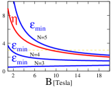
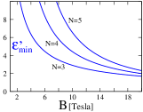
Figure 1: (left) $\eta$ and $\epsilon_{\text{min}}$ (for $n=3,4,5$ layer graphene), as a function of magnetic field $B$. To realize non-Abelian states, we need $\eta\gg 1$ and effective dielectric constant $\epsilon\gg\epsilon_{\text{min}}$. (right) $\epsilon^{\prime}_{\text{min}}$ for $n=3,4,5$ layer graphene.

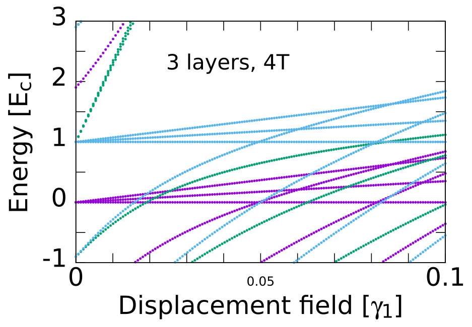
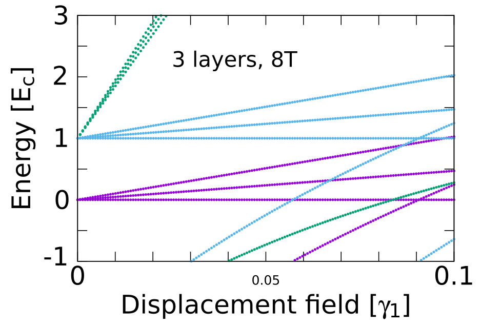
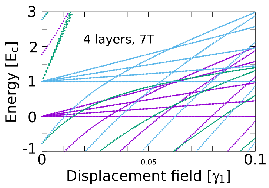
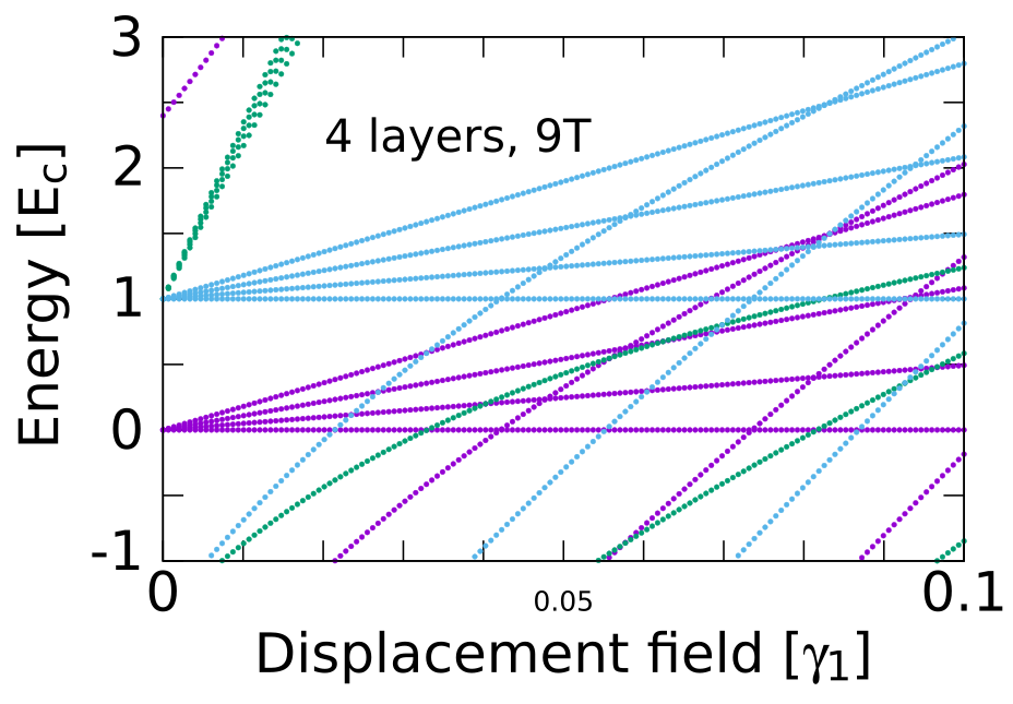
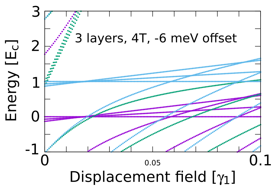
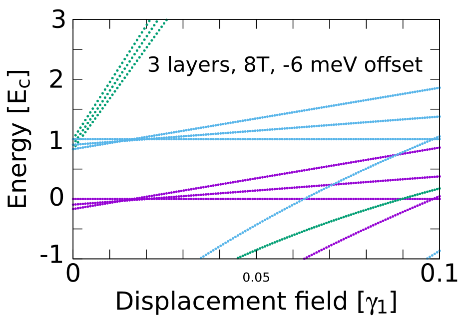
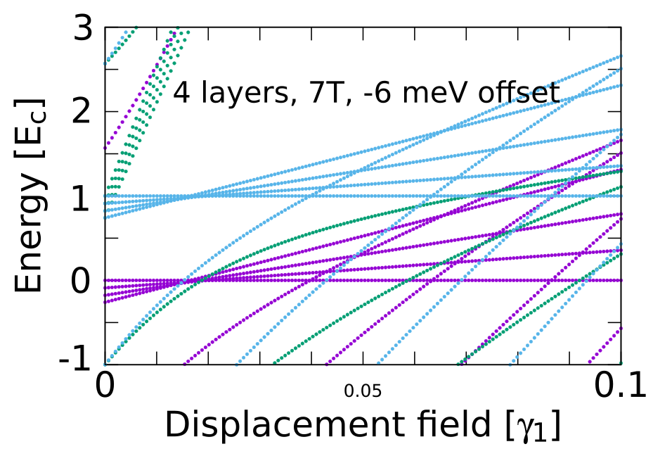
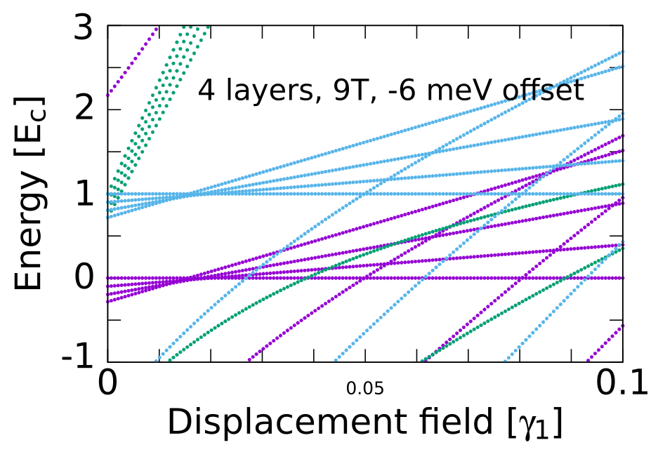
Figure 2: (top row) Effect of displacement field on single-particle Landau levels for three- and four-layer graphene. The displacement field (horizontal axis) is measured by interlayer potential energy difference in unit of interlayer hopping $\gamma_{1}=0.3eV$. The Landau level energy (vertical axis) is ploted in unit Coulomb energy $E_{c}=\frac{e^{2}}{\epsilon l_{B}}$ with $\epsilon=10$. The spin-up top-layer Landau levels are plotted in purple color. The spin-down top-layer Landau levels are plotted in blue color are shift up by Coulomb energy to simulate exchange effect. The bottom-layer Landau levels are plotted in green color are shift up by Coulomb energy as well to simulate exchange effect. The four plots are for (layer number, magnetic field) = $(3,\ 4$ Tesla), $(3,\ 8$ Tesla), $(4,\ 7$ Tesla), $(4,\ 9$ Tesla). (bottom row) The same as above, except the electron potential energy for different layers are offset by $(0,-6,0)$ meV or $(0,-6,-6,0)$ meV.

Also the Coulomb energy at magnetic length $l_{B}=\sqrt{2\pi\hbar c/eB}=643/\sqrt{B[\mathrm{Tesla}]}$Å  is about

$$\frac{e^{2}}{\epsilon l_{B}}=\frac{260}{\epsilon}\sqrt{B[\text{Tesla}]}\text{K}^{\circ}\equiv E_{c},$$ (20)

where $\epsilon$ is the dielectric constant – the reduction factor of the Coulomb interaction. We need interaction for electrons not in the surface layer to be less than the Landau-level energy gap: $\frac{n-1}{\eta^{2}}\frac{e^{2}}{\epsilon l_{B}}\ll\Delta$, or

$$\epsilon\gg 0.65\frac{(n-1)(\eta+1)(1.4+\eta)^{n-1}}{(\eta+2.5n-4)\eta^{2}\sqrt{n!}}\equiv\epsilon_{\text{min}}$$ (21)

so that the modified wave function (15) is a good approximation of ground state. We also like to have the Coulomb energy be less than the Landau-level energy gap $\frac{e^{2}}{\epsilon l_{B}}<\Delta$ so that the fill Landau levels below the degenerate Landau levels do not have a net non-zero $SU(4)$ quantum number due the exchange effect of the Coulomb interacton. This requires

$$\epsilon>0.65\frac{(\eta+1)(1.4+\eta)^{n-1}}{(\eta+2.5n-4)\sqrt{n!}}\equiv\epsilon^{\prime}_{\text{min}}$$ (22)

The conditions to realize non-Abelian states are summarized in Fig. 1. We see that those conditions are well satisfied for three-layer graphene with magnetic field $B\in[2,9]$ Tesla ($\eta\gtrsim 3$ and $\epsilon/\epsilon_{\text{min}}\gtrsim 10$), since the effective dielectric constant is about $\epsilon=10$. For four-layer graphene, the conditions are satisfied for magnetic field $B\in[5,9]$ Tesla ($\eta\gtrsim 3$ and $\epsilon/\epsilon_{\text{min}}\gtrsim 5$). While for five-layer graphene, the magnetic field needs to be $B\sim 10$ Tesla, where the conditions are barely satisfied ($\eta\sim 2.8$ and $\epsilon/\epsilon_{\text{min}}\sim 2.8$). It will be interesting to see if the $SU(2)_{2}$, $SU(3)_{2}$, $SU(2)_{3}$, non-Abelian QH states are realized by 3,4,5-layer graphene, respectively.

The effect of perpendicular electric field: We computed single-particle Landau levels for three- and four-layer graphene in presence of displacement field and offset of electron potential energy in different layers (see Fig. 2). The exchange effect of Coulomb energy can be simulated by energy splitting between up-spin top-layer Landau levels and other Landau levels. Both sets of Landau levels are ploted in Fig. 2. Note that the other Landau levels include down-spin top-layer, up-spin bottom-layer, and down-spin bottom-layer. We have assume the exchange splitting is the same for those three sets of Landau levels, since we only like to give a rough estimate.

At zero displacement field, the up-spin top-layer Landau levels (purple) near zero energy are partially filled. For three layer graphene at $B=8$ Tesla, we see that, as interlayer potential energy difference reaches $\sim 0.06\gamma_{1}=18$meV, the degenerate Landau levels have a splitting of order of Coulomb energy $\frac{e^{2}}{\epsilon l_{B}}$. Also other Landau levels start to cross the degenerate Landau levels. Both effects may destabilize the non-Abelian state discussed in this paper. At $B=4$ Tesla, the non-Abelian state may be destabilized when interlayer potential energy difference reachs $\sim 0.02\gamma_{1}=6$meV, due to Landau level crossing.

For four layer graphene at $B=9$ ($B=7$) Tesla, the non-Abelian state may destabilize when interlayer potential energy difference reaches $\sim 0.03\gamma_{1}=9$meV ($\sim 0.01\gamma_{1}=3$meV).

We would like to thank Long Ju, Patrick Ledwith, Andrea Young, Yuan-Bo Zhang, and Jun Zhu for very helpful discussions and comments. X.-G.W was partially supported by NSF grant DMR-2022428 and by the Simons Collaboration on Ultra-Quantum Matter, which is a grant from the Simons Foundation (651446, XGW).

References

- Laughlin [1983] R. B. Laughlin, Anomalous quantum Hall effect: An incompressible quantum fluid with fractionally charged excitations, Phys. Rev. Lett. 50, 1395 (1983).
- Tsui et al. [1982] D. C. Tsui, H. L. Stormer, and A. C. Gossard, Two-dimensional magnetotransport in the extreme quantum limit, Phys. Rev. Lett. 48, 1559 (1982).
- de Picciotto et al. [1997] R. de Picciotto, M. Reznikov, M. Heiblum, V. Umansky, G. Bunin, and D. Mahalu, Direct observation of a fractional charge, Nature 389, 162 (1997).
- Leinaas and Myrheim [1977] J. M. Leinaas and J. Myrheim, On the theory of identical particles, Nuovo Cim B 37, 1 (1977).
- Wilczek [1982] F. Wilczek, Quantum mechanics of fractional-spin particles, Phys. Rev. Lett. 49, 957 (1982).
- Halperin [1984] B. I. Halperin, Statistics of quasiparticles and the hierarchy of fractional quantized Hall states, Phys. Rev. Lett. 52, 1583 (1984).
- Arovas et al. [1984] D. Arovas, J. R. Schrieffer, and F. Wilczek, Fractional statistics and the quantum Hall effect, Phys. Rev. Lett. 53, 722 (1984).
- Wu [1984] Y.-S. Wu, General theory for quantum statistics in two dimensions, Phys. Rev. Lett. 52, 2103 (1984).
- Wen [1989] X.-G. Wen, Vacuum degeneracy of chiral spin states in compactified space, Phys. Rev. B 40, 7387 (1989).
- Wen [1990] X.-G. Wen, Topological orders in rigid states, Int. J. Mod. Phys. B 04, 239 (1990).
- Wen and Niu [1990] X.-G. Wen and Q. Niu, Ground-state degeneracy of the fractional quantum Hall states in the presence of a random potential and on high-genus Riemann surfaces, Phys. Rev. B 41, 9377 (1990).
- Goldin et al. [1985] G. A. Goldin, R. Menikoff, and D. H. Sharp, Comments on “general theory for quantum statistics in two dimensions”, Phys. Rev. Lett. 54, 603 (1985).
- Moore and Seiberg [1989] G. Moore and N. Seiberg, Classical and quantum conformal field theory, Commun.Math. Phys. 123, 177 (1989).
- Witten [1989] E. Witten, Quantum field theory and the Jones polynomial, Commun.Math. Phys. 121, 351 (1989).
- Kitaev [2006] A. Kitaev, Anyons in an exactly solved model and beyond, Ann. Phys. 321, 2 (2006), arXiv:cond-mat/0506438 .
- Jain [1990] J. K. Jain, Theory of the fractional quantum Hall effect, Phys. Rev. B 41, 7653 (1990).
- Wen [1991] X.-G. Wen, Non-Abelian statistics in the FQH states, Phys. Rev. Lett. 66, 802 (1991).
- Wen [1999] X.-G. Wen, Projective construction of non-Abelian quantum Hall liquids, Phys. Rev. B 60, 8827 (1999), arXiv:cond-mat/9811111 .
- Blok and Wen [1992] B. Blok and X.-G. Wen, Many-body systems with non-abelian statistics, Nucl. Phys. B 374, 615 (1992).
- Moore and Read [1991] G. Moore and N. Read, Nonabelions in the fractional quantum hall effect, Nucl. Phys. B 360, 362 (1991).
- Wen [1993] X.-G. Wen, Topological order and edge structure of =1/2 quantum Hall state, Phys. Rev. Lett. 70, 355 (1993).
- Bonderson et al. [2011] P. Bonderson, V. Gurarie, and C. Nayak, Plasma analogy and non-abelian statistics for ising-type quantum Hall states, Phys. Rev. B 83, 075303 (2011), arXiv:1008.5194 .
- Willett et al. [1987] R. Willett, J. P. Eisenstein, H. L. Störmer, D. C. Tsui, A. C. Gossard, and J. H. English, Observation of an even-denominator quantum number in the fractional quantum Hall effect, Phys. Rev. Lett. 59, 1776 (1987).
- Xia et al. [2004] J. S. Xia, W. Pan, C. L. Vicente, E. D. Adams, N. S. Sullivan, H. L. Stormer, D. C. Tsui, L. N. Pfeiffer, K. W. Baldwin, and K. W. West, Electron Correlation in the Second Landau Level: A Competition Between Many Nearly Degenerate Quantum Phases, Phys. Rev. Lett. 93, 176809 (2004), arXiv:cond-mat/0406724 .
- Dolev et al. [2008] M. Dolev, M. Heiblum, V. Umansky, A. Stern, and D. Mahalu, Observation of a quarter of an electron charge at the = 5/2 quantum Hall state, Nature 452, 829 (2008), arXiv:0802.0930 .
- Banerjee et al. [2018] M. Banerjee, M. Heiblum, V. Umansky, D. E. Feldman, Y. Oreg, and A. Stern, Observation of half-integer thermal Hall conductance, Nature 559, 205 (2018), arXiv:1710.00492 .
- Ki et al. [2014] D.-K. Ki, V. I. Fal’ko, D. A. Abanin, and A. F. Morpurgo, Observation of Even Denominator Fractional Quantum Hall Effect in Suspended Bilayer Graphene, Nano Letters 14, 2135 (2014), arXiv:1305.4761 .
- Zibrov et al. [2017] A. A. Zibrov, C. R. Kometter, H. Zhou, E. M. Spanton, T. Taniguchi, K. Watanabe, M. P. Zaletel, and A. F. Young, Robust fractional quantum Hall states and continuous quantum phase transitions in a half-filled bilayer graphene Landau level, Nature 549, 360 (2017), arXiv:1611.07113 .
- Huang et al. [2022] K. Huang, H. Fu, D. R. Hickey, N. Alem, X. Lin, K. Watanabe, T. Taniguchi, and J. Zhu, Valley Isospin Controlled Fractional Quantum Hall States in Bilayer Graphene, Physical Review X 12, 031019 (2022), arXiv:2105.07058 .
- Levin and Halperin [2009] M. Levin and B. I. Halperin, Collective states of non-Abelian quasiparticles in a magnetic field, Phys. Rev. B 79, 205301 (2009), arXiv:0812.0381 .
- Yang et al. [2022] J. Yang, G. Chen, T. Han, Q. Zhang, Y.-H. Zhang, L. Jiang, B. Lyu, H. Li, K. Watanabe, T. Taniguchi, Z. Shi, T. Senthil, Y. Zhang, F. Wang, and L. Ju, Spectroscopy signatures of electron correlations in a trilayer graphene/hBN moiré superlattice, Science 375, 1295 (2022), arXiv:2202.12330 .
- Han et al. [2023] T. Han, Z. Lu, G. Scuri, J. Sung, J. Wang, T. Han, K. Watanabe, T. Taniguchi, H. Park, and L. Ju, Correlated Insulator and Chern Insulators in Pentalayer Rhombohedral Stacked Graphene 10.48550/arXiv.2305.03151 (2023), arXiv:2305.03151 .
- Liu et al. [2023] K. Liu, J. Zheng, Y. Sha, B. Lyu, F. Li, Y. Park, Y. Ren, K. Watanabe, T. Taniguchi, J. Jia, W. Luo, Z. Shi, J. Jung, and G. Chen, Interaction-driven spontaneous broken-symmetry insulator and metals in ABCA tetralayer graphene, (2023), arXiv:2306.11042 .
- Wu et al. [2017] Y.-H. Wu, T. Shi, and J. K. Jain, Non-Abelian Parton Fractional Quantum Hall Effect in Multilayer Graphene, Nano Letters 17, 4643 (2017), arXiv:1603.02153 .
- Min and MacDonald [2008] H. Min and A. H. MacDonald, Chiral decomposition in the electronic structure of graphene multilayers, Phys. Rev. B 77, 155416 (2008), arXiv:0711.4333 .
- Zhang et al. [2008] L. M. Zhang, Z. Q. Li, D. N. Basov, M. M. Fogler, Z. Hao, and M. C. Martin, Determination of the electronic structure of bilayer graphene from infrared spectroscopy, Phys. Rev. B 78, 235408 (2008), arXiv:0809.1898 .