Generating Hard Ising Instances With Planted Solutions Using Post-Quantum Cryptographic Protocols

Abstract

In this paper we present a novel method to generate hard instances with planted solutions based on the public-private McEliece post-quantum cryptographic protocol. Unlike other planting methods rooted in the infinite-size statistical analysis, our cryptographic protocol generates instances which are all hard (in cryptographic terms), with the hardness tuned by the size of the private key, and with a guaranteed unique ground state. More importantly, because of the private-public key protocol, planted solutions cannot be easily recovered by a direct inspection of the planted instances without the knowledge of the private key used to generate them, therefore making our protocol suitable to test and evaluate quantum devices without the risk of “backdoors” being exploited.

I Introduction

With the advent of more competitive (either quantum Arute et al. (2019); Morvan et al. (2023); Kim et al. (2023), quantum inspired Kim et al. (2021); Aramon et al. (2019); Zhu et al. (2015) or post-Von Neumann Mohseni et al. (2022); Sao et al. (2019); Traversa and Di Ventra (2015); Adleman (1994)) technologies for the optimization of classical cost functions, it is becoming of utmost importance to identify classes of instances which are well suited to transversally benchmark such devices. One of the major challenges in designing planted problems is the generation of instances which are hard to optimize: indeed, planting a desired solution may affect the energy landscape of the instance, making it more convex and therefore easier to explore. Another important aspect that may affect the hardness of planted problems is the number of solutions: while it is guaranteed that the planted configuration is a solution, the planting protocol may introduce multiple solutions that would make the instance easier to solve.

In this work we introduce a way of generating Ising instances with one unique planted solution, whose hardness against optimization algorithms is derived from the robustness of the McEliece cryptographic protocol that is used to create them. The rest of the paper is organized as follows: in Section II we give an overview of the currently available planting methods for Ising Hamiltonians, in Section III we review linear codes, and the McEliece cryptographic protocol. Section IV shows how to generate hard instances of Ising Hamiltonians with planted solutions by recasting the McEliece protocol in Ising spin language, while Section V uses the machinery of statistical physics to illustrate why energy landscapes analogous to the ones exhibited these hard instances should be difficult to explore for stochastic local search algorithms.

II Overview of Existing Planting Methods

For Constraint Satisfaction Problems (CSPs) like the graph coloring Papadimitriou and Steiglitz (1998); Sipser (1996) and the SAT problem Biere et al. (2009), solutions can be planted by using the “quiet” planting technique Qu and Potkonjak (1999); Barthel et al. (2002); Krzakala and Zdeborová (2009); Zdeborová and Krzakala (2011); Krzakala et al. (2012); Sicuro and Zdeborová (2021): constraints that satisfy the desired planted configuration are added until the required density of constraints is achieved. Similarly to random CSPs Mézard et al. (2002); Zdeborová and Krzakala (2007), planted CSPs have different phase transition by varying the density of constraints Zdeborová and Krzakala (2007); Krzakala and Zdeborová (2009); Ricci-Tersenghi et al. (2019); Semerjian et al. (2020): while the “satisfiability” threshold is of course suppressed, phase transitions related to the hardness of the instances, such as the “freezing” transition Zdeborová and Krzakala (2007), are preserved in planted instances. In particular, in frozen planted instances, solutions are all clustered into a single component which make the instance hard to optimize Zdeborová and Mézard (2008). While the quiet planting can be used to quickly generate planted instances, properties like the hardness of the instances and the number of solutions are only true for the “typical” case and in the limit of large number of variables, making the technique less valuable for small-scale and mid-scale benchmarks.

Similar to the quiet planting, the “patch” planting is a technique used to plant solutions for cost functions where not all the constraints must be satisfied at the same time Denchev et al. (2016); Hen et al. (2015); Wang et al. (2017); Hamze et al. (2018); Perera et al. (2020). More precisely, multiple sub-systems with a known solution are “patched” together by properly applying hard constraints between sub-systems. Solutions for each sub-systems are found by either brute force or using other optimization techniques, and global solutions are obtained by patching together solutions from all the sub-systems. The hardness of the patch planted instances is then tuned by increasing the size and the hardness of the sub-systems Wang et al. (2017). Even if the patch planting technique can generate instances rather hard to optimize Hamze et al. (2018), one of the main downside of the technique is that a direct inspection of the instances may easily reveal the solution. A random permutation of the variable indexes could mitigate the problem, but the use of cluster techniques Zhu et al. (2015) or the knowledge of the pre-permutation layout may still be used to identify each sub-systems.

Another common technique to plant solutions in combinatorial optimization problems consists in using exactly solvable models that present phase transitions. The simplest example is the problem of solving linear equation on the binary field (also called XORSAT Hen (2019)). More precisely, given a binary matrix $\mathbf{A}$ of size $M\times N$, with $M$ being the number of equations and $N$ the number of variables, the XORSAT problem consists in finding the solution $x$ such that $\mathbf{A}x=0$, where the identity is modulo 2. If $M>N$, the fundamental theorem of the linear algebra ensures that there are at least $2^{M-N}$ solutions. As for many other CSPs, XORSAT instances undergo different phase transition by changing the density of constraints $M/N$, with the hardest instances being close to the satisfiability threshold Mézard et al. (2002). While XORSAT instances are known to be hard to optimize using local heuristics, the simple knowledge of $\mathbf{A}$ (regardless any permutation of the variable indexes) is enough to find the set of solutions by using the Gaussian elimination.

A similar strategy is used in the generation of the Wishart instances Hamze et al. (2020). In this case, real valued matrices $\mathbf{W}\in\mathbb{R}^{k\times N}$ are chosen such that $\mathbf{W}x^{*}=0$ for the desired binary variable. Therefore, the corresponding binary cost function $H(x)=\frac{1}{2}x^{T}\mathbf{W}^{T}\mathbf{W}x=\frac{1}{2}\sum_{ij}J_{ij}x_{i}x_{j}$ is guaranteed to have $x^{*}$ as solution. The hardness of the Wishart instances is tuned by properly choosing the ratio $\alpha=k/N$, with an easy-hard-easy pattern by increasing $\alpha$. Interestingly, the study of the Thouless-Anderson-Palmer (TAP) equations Thouless et al. (1977) applied to the Wishart problem shows the existence of a first order phase transition, making the Wishart instances hard to optimize for local heuristics. Moreover, unlike many other planting techniques, the Wishart instances are fully-connected and hard to optimize, even for a small number of variables. However, the hardness of the Wishart instances also depends on the digit precision of $\mathbf{W}$, making it less suitable for devices with a limited precision. Moreover, the number of solutions, which also may affect the hardness of the Wishart instances, cannot be determined except by an exhaustive enumeration and cannot be fixed in advance.

In King et al. (2019), the fact that local heuristics have troubles to optimize frustrated loop is used to generate random instances with a known ground state, and hence the name Frustrated Cluster Loops (FCL). The ruggedness $R$ of an FCL instance is how many loops a single variable is involved in, and it determines the hardness of the instances. Unfortunately, cluster methods easily identify these frustrated loops and therefore solve the FCL instances efficiently Mandra et al. (2016, 2017, 2019). A variation of the FCL planting method has been used in Mandra and Katzgraber (2018) to generate hard instances. In this case, FCL instances are embedded on a Chimera graph with an embedding cost tuned by $\lambda$. The name Deceptive Cluster Loops (DCL) derives from the fact that for $\lambda$ small enough, the ground state of DCL instances is mappable to the ground state of an equivalent 2D model, while for $\lambda$ large to the ground state of a fully connected model. The hardness is then maximized at the transition between the two limits. Unfortunately, while generating hard instances, the ground state can be determined only at the extrema of $\lambda$.

One of the first example of the use of a private/public key protocol to generate hard instances can be found in Merkle and Hellman (1978). More precisely, the authors of the paper use the subset sum problem Sipser (1996), where a subset of a set of number $\Omega=\{\omega_{1},\,\omega_{2},\ \ldots,\ \omega_{N}\}$ must be found such that their sum equals a given value $c$. The problem is known to be NP-Complete, and its quadratic binary cost function can be expressed as $H(x)=\sum_{i=1}^{n}\left(\omega_{i}x_{i}-c\right)^{2}$. However, the subset sum problem as a pseudopolynomial time algorithm Papadimitriou (2003) which takes $\mathcal{O}(n\omega^{*})$ memory, with $\omega^{*}$ being the largest value $\omega_{i}$ in the set. The Merkle-Hellman encryption algorithm works by using two sets of integers: the “private” key $\Omega$, which is a superincreasing set of numbers, and a “public” key $\Omega^{\prime}$, which is defined as $\omega^{\prime}_{i}=r\omega_{i}\ \text{mod}\ q$, with $q>\sum_{i}\omega_{i}$ and $r$ being a random integer such that $r$ and $q$ are coprime. The values $r$ and $q$ are also kept secret, A message $m_{i}$ of $N$ bits is then encrypted as $c=\sum_{i}m_{i}\omega^{\prime}_{i}$. On the one hand, without the knowledge of the private key, one must optimize the quadratic binary cost function $H(x)=\left(\omega^{\prime}_{i}x_{i}-c\right)^{2}$ in order to find the encoded message. On the other hand, thanks to the fact that $\Omega$ is a set of superincreasing numbers and that the inverse of $r$ modulo $q$ can be efficiently found using the extended Euclidean algorithm, one can easily recover the binary message without the optimization of $H(x)$. The fact that the binary message $m_{i}$ is recoverable immediately guarantees that the ground state must be unique. Unfortunately, the use of superincreasing sequence of numbers makes the Merkle-Hellman protocol vulnerable to attacks Shamir (1982) by just looking at the public key $\Omega^{\prime}$. Moreover, the complexity from the computational point of view depends on $\omega^{*}$ which sets the minimum digit precision for the set $\Omega$. That is, exponentially hard integer partition instances require exponentially large $\omega_{i}$, limiting the use of this protocol on devices with limited precision.

Recently, the integer factorization problem has been used to generate hard binary instances Pirnay et al. (2022); Szegedy (2022). More precisely, given two large prime numbers $a$ and $b$ of $N-$binary digits, the binary cost function is defined as $H(x,\ y)=\left[\left(\sum_{i=1}^{N}2^{i}x_{i}\right)\left(\sum_{i=1}^{N}2^{i}y_{i}\right)-c\right]^{2}$, with $c=ab$. Instances based on factoring becomes exponentially hard by increasing the number of binary digits $N$. While no known classical algorithms are known to efficiently solve $H(x,\ y)$ without actually optimizing the binary cost function, factoring is vulnerable to quantum attacks via the Shor algorithm Shor (1999). Moreover, the optimization of the binary cost function $H(x,\,y)$ requires an exponential precision, making such instances unsuitable for devices with limited precision.

III Background on Linear Codes

To simplify the reading, for the rest of the paper it is assumed, unless otherwise specified, that all matrices and linear algebra operations take place over the finite field $\mathbb{F}_{2}\equiv\mathbb{Z}/2\mskip 1.5mu\mathbb{Z}$. Let us define the generator matrix $\mathbf{G}\in\mathbb{F}_{2}^{\,k\times N}$ of a linear code $C$, with $k\leq N$, and its check matrix $\mathbf{K}\in\mathbb{F}_{2}^{\,(N-k)\times n}$ such that $\mathbf{H}\mathbf{G}^{T}=0$. A message $x\in\mathbb{F}_{2}^{\,k}$ can be then encoded as a string $y\in\mathbb{F}_{2}^{\,N}$ via

$$y\equiv x\,\mathbf{G}.$$ (1)

The distance of $C$ is defined as the minimum Hamming weight among all the possible non-zero codewords, that is:

$$d\equiv\min_{x\in\mathbb{F}_{2}^{\,k},\ x\not=0}\left\|x\,\mathbf{G}\right\|,$$ (2)

where $\|\cdot\|$ indicate the Hamming distance. A linear code of distance $d$ can detect up to $d-1$ errors and correct up to $(d-1)/2$ errors. Indeed, let us define a vector $\epsilon$ with $t=\left\lvert\epsilon\right\rvert$ ones. The error would alter the encoded message as:

$$y^{\prime}=x\,\mathbf{G}+\epsilon$$ (3)

Since $x\,\mathbf{G}\mathbf{H}^{T}=0$ by construction, applying the parity check to $y^{\prime}$ one gets:

$$y^{\prime}\,\mathbf{H}^{T}=\epsilon\,\mathbf{H}^{T}.$$ (4)

However, if $t<d$, $\epsilon$ cannot be a codeword of $C$ and therefore $\epsilon\,\mathbf{H}^{T}\not=0$, that is the code $C$ can detect up to $d-1$ errors. An error can be instead corrected if, for a given syndrome $\epsilon\,\mathbf{H}^{T}$, it is possible to unequivocally identify $\epsilon$. This is the case when two errors $\epsilon_{1}$ and $\epsilon_{2}$ produce two different syndromes. More precisely

$$\epsilon_{1}\,\mathbf{H}^{T}\not=\epsilon_{2}\,\mathbf{H}^{T}\Rightarrow\left(\epsilon_{1}-\epsilon_{2}\right)\mathbf{H}^{T}\not=0,$$ (5)

that is $\epsilon_{1}-\epsilon_{2}$ is not a codeword of $C$. However, if $\epsilon_{1}$ and $\epsilon_{2}$ have respectively $t_{1}$ and $t_{2}$ errors, their sum cannot have more than $t_{1}+t_{2}$ errors, implying that two syndromes can be distinguished only if the number of errors is smaller than $t\leq(d-1)/2$.

III.1 McEliece Public/Private Key Protocol

In 1978, Robert McEliece discovered that linear codes $C$ can be used as asymmetric encryption schemes McEliece (1978). While not getting much acceptance from the cryptographic community because of its large private/public key and being vulnerable to attacks using information-set decoding Bernstein et al. (2008), the McEliece has recently gained more traction as a “post-quantum” cryptographic protocol, as it is immune to the Shor’s algorithm Dinh et al. (2011). At the time of writing, NIST has promoted the McEliece protocol to the phase 4 of its post-quantum cryptographic standardization NIST .

In the McEliece protocol, the private key consists of a linear code $C$ of distance $d$ (with $\mathbf{G}$ and $\mathbf{H}$ being its generator matrix and check matrix respectively), a (random) permutation matrix $\mathbf{P}\in\mathbb{F}_{2}^{\,N\times N}$, and a (random) non-singular matrix $\mathbf{S}\in\mathbb{F}_{2}^{\,k\times k}$. On the other hand, the public key is defined as a new generator matrix $\mathbf{G}^{\prime}=\mathbf{S}\mathbf{G}\mathbf{P}$ with distance $d$. Indeed, $\|x\,\mathbf{G}^{\prime}\|=\|x\,\mathbf{S}\mathbf{G}\mathbf{P}\|=\|x\,\mathbf{S}\mathbf{G}\|$ since the Hamming weight is invariant by permutation, and

$$\min_{x\in\mathbb{F}_{2}^{\,k},\ x\not=0}\left\|x\,\mathbf{S}\mathbf{G}\right\|=\min_{y\in\mathbb{F}_{2}^{\,k},\ y\not=0}\left\|y\,\mathbf{G}\right\|=d,$$ (6)

where we used the fact that $\mathbf{S}$ is non-singular and $y=x\,\mathbf{S}$. It is important to notice that it is hard to recover the original generator matrix $\mathbf{G}$ from $\mathbf{G}^{\prime}$ without the knowledge of $\mathbf{P}$ and $\mathbf{S}$. In the McEliece protocol, $\mathbf{S}$ is used to “obfuscate” the original generator matrix $\mathbf{G}$ by scrambling it. In the next Section, we will use a similar concept to create hard instances with a known and unique ground state.

The message encoding is then obtained by applying the public key $\mathbf{G}^{\prime}$ to an arbitrary message $q\in\mathbb{F}_{2}^{\,k}$ and randomly flipping a number $t=(d-1)/2$ of bits, that is:

$$q^{\prime}\equiv q\,\mathbf{G}^{\prime}+\epsilon,$$ (7)

with $\|\epsilon\|=t$. If the private key is known, the message $q$ can be recovered by observing that $\epsilon^{\prime}=\epsilon\,\mathbf{P}^{-1}$ preserves the number of errors. Therefore the permuted encoded message $q^{\prime}\mathbf{P}^{-1}=q\,\mathbf{S}\mathbf{G}+\epsilon^{\prime}$ can be “corrected” using the parity check $\mathbf{H}$. Indeed

$$q^{\prime}\mathbf{P}^{-1}\mathbf{H}^{T}=\left(q\,\mathbf{S}\mathbf{G}+\epsilon^{\prime}\right)\mathbf{H}^{T}=\epsilon^{\prime}\mathbf{H}^{T}$$ (8)

by construction. Because $\|\epsilon^{\prime}\|\leq(d-1)/2$, one can identify $\epsilon^{\prime}$ and remove it from the permuted message and therefore recover $q\,\mathbf{S}$. Finally, the encoded message can be recovered by multiplying $\mathbf{S}^{-1}$ to the right of $q\,\mathbf{S}$.

Without the knowledge of the private key, the message $q^{\prime}$ can be decoded by using the maximum likelihood estimation:

$$q=\underset{x\in\mathbb{F}_{2}^{\,k}}{\rm argmin}\left\|q^{\prime}-x\,\mathbf{G}^{\prime}\right\|.$$ (9)

Recalling that Eq. (9) is invariant by non-singular transformations $x\leftarrow x\,\mathbf{Q}$ with $\mathbf{Q}\in\mathbb{F}_{2}^{\,k\times k}$, it is always possible to reduce $\mathbf{G}^{\prime}$ to its normal form $\mathbf{Q}^{-1}\mathbf{G}^{\prime}=\left(\mymathbb{1}\ \mathbf{W}\right)$, with $\mymathbb{1}$ being the identity matrix of size $k\times k$ and $\mathbf{W}\in\mathbb{F}_{2}^{\,k\times(N-k)}$.

Since the encrypted message $q$ is recoverable, it is guaranteed that one and only one configuration exists that minimizes Eq. (9). The hardness of the McEliece protocol depends on the size of the codespace and the distance $d$ of the code $C$. By properly choosing $k$ and $d$, it is possible to generate instances with a tunable hardness.

IV Generating Hard Instances from Linear Codes

In this section we will show that the McEliece protocol can be used to generate hard instances of a disordered Ising Hamiltonian. More precisely, we are interested in generating $p$-local Ising instances of the form:

$$H(\sigma)=\sum_{i=1}^{M}J_{i}\,\sigma_{i_{1}}\cdots\,\sigma_{i_{p}}$$ (10)

with $p\geq 1$, $1\leq i_{1},\,\ldots,\,i_{p}\leq k$, $\sigma=\{\pm 1\}^{k}$ and couplings $J_{i_{1}\cdots i_{p}}\in\mathbb{R}$. To achieve this goal, it suffices to show that the finding a solution of the maximum likelihood equation in Eq. (9) is equivalent to finding the ground state of the $p-$spin Ising instance (10).

Let us define $\mathbf{G}^{\prime}_{i}$ the $i$-th column of $\mathbf{G}^{\prime}$. Therefore, it is immediate to show that:

$$W(x)=\|q^{\prime}-x\,\mathbf{G}^{\prime}\|=\sum_{i=1}^{N}\|q^{\prime}_{i}-x\cdot g^{\prime}_{i}\|,$$ (11)

where the operations inside $\|\cdot\|$ are intended modulo $2$, while the sum is over $\mathbb{R}$. By mapping $\sigma_{i}=1-2x_{i}$, and by recalling that

$$(x_{1}+\cdots+x_{k})\!\!\mod 2 =(1-\sigma_{1}\cdots\sigma_{k})/2,$$ (12a)

$$(x_{1}+\cdots+x_{k}+1)\!\!\mod 2 =(1+\sigma_{1}\cdots\sigma_{k})/2,$$ (12b)

Eq. (11) becomes:

$$W(x) =\sum_{i=1}^{N}\|q^{\prime}_{i}-x\cdot\mathbf{G}^{\prime}_{i}\|=\sum_{i=1}^{N}\left[1-(-1)^{q^{\prime}_{i}}\sigma_{i_{1}}\cdots\sigma_{i_{p_{i}}}\right]$$

$$=-\sum_{i=1}^{N}(-1)^{q^{\prime}_{i}}\sigma_{i_{1}}\cdots\sigma_{i_{p_{i}}}+N=H(\sigma)+N,$$ (13)

with $\{i_{1},\,\ldots,\,i_{p_{i}}\}$ being the indices of the non-zero elements of $\mathbf{G}^{\prime}_{i}$, and $p_{i}=\lvert g^{\prime}_{i}\rvert$ their number. It is interesting to observe that the indices of the interactions $\{i_{1},\,\ldots,\,i_{p_{i}}\}$ are fixed after choosing the private key $\{\mathbf{G},\ \mathbf{H},\ \mathbf{P},\ \mathbf{S}\}$. However, multiple random instances can be generated by providing different $q^{\prime}=q\mathbf{G}^{\prime}+\epsilon$, which will only change the sign of the interactions. It is important to emphasize that, if the private key is properly chosen, every instance $H(\sigma)$ will be hard to optimize, regardless the choice of $q^{\prime}$. This is consistent with fact that $p$-local instances with randomly chosen $J_{i_{1}\cdots i_{p}}=\pm 1$ and $p\geq 2$ are NP-Complete. However, unlike the case when the couplings are randomly chosen, $p$-local instances generated using the McEliece protocol have a guaranteed unique optimal value, which is known in advance (that is, $q$).

Since we don’t need to apply $\mathbf{S}^{-1}$ to obtain $H(\sigma)$ in Eq. (IV), we can relax the request to have obfuscation matrix $\mathbf{S}$ being non-singular. In particular, the number of solutions of the $H(\sigma)$ will depend on the size of the kernel of $\mathbf{S}$. Indeed, not having $\mathbf{S}$ invertible implies that $\mathbf{S}$ has a non-empty kernel and, therefore, two distinct messages $q_{1}$ and $q_{2}$ may have the same encrypted message, $q^{\prime}_{1}$ and $q^{\prime}_{2}$. Consequently, the $p-$spin instance $H(\sigma)$ will have as many optimal configuration as the number of collisions for a given message $q$, that is the number of elements in $\mathbf{S}$ kernel.

IV.1 Reduction to the 2-local Ising Model

Since the $p$-local Ising model is NP-Complete for $p\geq 2$, any optimization problem in the NP class can be mapped onto it. However, almost all post-Von Neumann Mohseni et al. (2022); Sao et al. (2019); Traversa and Di Ventra (2015); Adleman (1994) technologies can only optimize $p$-local Ising instances with either $p=2$ or $p=3$. Unfortunately, because of the random scrambling induced by $\mathbf{S}$, $\mathbf{G}^{\prime}$ is a dense matrix with $p_{i}\leq k$. Luckily, $p$-local couplings with $p>3$ can always be reduced to $p\leq 3$ by adding auxiliary variables.

For $p=3$, it is immediate to show that:

$$(-1)^{t}\sigma_{1}\cdots\sigma_{l}\sigma_{l+1}\cdots\sigma_{p}=\\ \min_{\omega=\pm 1}\left[\sigma_{1}\cdots\sigma_{l}\,\omega+(-1)^{t}\,\omega\,\sigma_{l+1}\cdots\sigma_{p}\right]+1.$$ (14)

Thefore, reducing $\mathbf{G}^{\prime}$ to a $3$-local Ising instance would require no more than $k^{\prime}=k+\left(\left\lceil\frac{k}{2}\right\rceil-1\right)(N-k)$ spin variables and $n^{\prime}=k+\left\lceil\frac{k}{2}\right\rceil(n-k)$ couplings in the worst case scenario. Reducing a coupling from $p=3$ to $p=2$ requires the addition of another extra auxiliary spin for each $3$-local coupling. More precisely, since

$$\underset{\sigma_{1},\,\sigma_{2},\,\sigma_{3}=\pm 1}{\rm argmin}(-1)^{t}\sigma_{1}\sigma_{2}\sigma_{3}=\\ \underset{\sigma_{1},\,\sigma_{2},\,\sigma_{3}\,\omega=\pm 1}{\rm argmin}\left[\sigma_{1}+\sigma_{2}+(-1)^{t}\left(1-2w\right)\right]^{2},$$ (15)

it is possible to reduce $\mathbf{G}^{\prime}$ to up to $k^{\prime\prime}\equiv k(N-k+1)=\mathcal{O}(kN)$ spin variables and $N^{\prime\prime}\equiv N+k(n-k)=\mathcal{O}(kN)$ couplings in the worst case scenario.

IV.2 The Scrambling Protocol

In this Section we will show how we can use the “scrambling” of the codespace of $C$ induced by the non-singular matrix $\mathbf{S}$ to generate random hard $p$-local Ising instances with a known optimal configuration. To this end, it suffices to show that any $p-$spin Ising instance of the form Eq. (10) can always be reduce to a maximum likelihood problem as in Eq. (9).

Using the transformation in Eq. (12), the $p$-local Ising instance in Eq. (10) can be rewritten as:

$$H(x)=\sum_{i=1}^{M}{\rm abs}\left(J_{i}\right)(\Big{\|}x_{i}+\cdots+x_{i_{p}}+\\ +\frac{1+{\rm sgn}(J_{i})}{2}\Big{\|}-1\Big{)},$$ (16)

where ${\rm abs}(\cdot)$ and ${\rm sgn}(\cdot)$ are the absolute and sign functions respectively, and all operations inside $\lvert\cdot\rvert$ are modulo $2$. If we define $\mathbf{J}\in\mathbb{F}_{2}^{\,k\times M}$ the adjacency matrix of the couplings $J_{i_{1}\cdots i_{p}}$ such that $\mathbf{J}_{ai}=1$ if $a\in\{i_{1},\,\ldots,\,i_{p}\}$ and zero otherwise, Eq. (16) becomes

$$H(x)=\sum_{i=1}^{M}{\rm abs}\left(J_{i}\right)\Big{(}\Big{\|}x\cdot\mathbf{J}_{i}+\frac{1+{\rm sgn}(J_{i})}{2}\Big{\|}-1\Big{)},$$ (17)

where $\mathbf{J}_{i}$ is the $i$-th column of $\mathbf{J}$ and $x\in\mathbb{F}_{2}^{\,k}$. Observe that Eq. (17) is equivalent to the maximum likelihood in Eq. (9) when ${\rm abs}(J_{i})=1$ for all $i$. More importantly, it is immediate to see that, for any non-singular transformation, $\mathbf{S}$ an optimal configuration $x^{*}$ of $H(x)$ is mapped to $x^{*\prime}=x^{*}\mathbf{S}^{-1}$, preserving the number of optimal configurations. We can relax the condition of having $\mathbf{S}$ being non-singular. In this case, the number of optimal configurations is not preserved since

$$x^{*}=\left(x^{*\prime}+\xi\right)\mathbf{S}$$ (18)

for any $\xi$ belonging to the kernel space of $\mathbf{S}$. Once the adjacency matrix $\mathbf{J}^{\prime}=\mathbf{S}\,\mathbf{J}$ is scrambled, one can map Eq. (17) back to a $p-$spin Ising instance using the methodology presented in Section IV.1.

In the next Section we try to shed light on the reason why scrambling the configuration space $x$ with $\mathbf{S}$ produces instances which are hard to optimize for local heuristics.

V Random Scrambling of Energy Landscapes

In order to study the effect of energy scrambling over an Ising Hamiltonian, we show in this Section how various forms of energy scrambling — similar to the one induced by the scrambling matrix $\mathbf{S}$ of the McEliece protocol — can transform simple problems into significantly more complex ones by introducing a version of a phenomenon known in the statistical physics literature as “clustering” Mézard et al. (2005); Achlioptas and Ricci-Tersenghi (2006), where the solution space of a constraint optimization problem splits into a (typically exponential) number of “clusters”. This phenomenon is conjectured – on the basis of empirical evidence collected in the study of constraint satisfaction problems – to impair the performance of stochastic local search algorithms such as WalkSAT Coja-Oghlan et al. (2017) even though the precise connection between clustering and the theory of algorithmic hardness is still an active area of research, and not fully understood Gamarnik (2021); Angelini and Ricci-Tersenghi (2023).

In order to understand the algorithmic hardness of the system of Eq. (10) using the methods of statistical physics, one would like to study the typical properties of the energy landscape of the “disordered Hamiltonian” $H(\sigma)$ where the disordered couplings $J_{{i_{1}}\ldots i_{p}}$ are generated by e.g. a fixed choice of the linear code matrix $\mathbf{G}$ (one for each system size $N$), and the random choices for the permutation matrices $\mathbf{S},\mathbf{P}$. For this introductory work we limit ourselves to a simpler scenario that allows us focus on one component of the McEliece protocol: the effect of an energy scrambling matrix $\mathbf{S}$. In particular

1. We only consider the effect of one source of quenched disorder, i.e. a random scrambling matrix $\mathbf{S}$. As shown in Section IV.2, the effect of changing the $\mathbf{S}$ permutation matrix in the McEliece protocol (for given $\mathbf{G}$ and $\mathbf{P}$) is to shuffle the energies of the states of the system.

2. Instead of considering the effects that $\mathbf{S}$ has on the energy landscape of a reference Hamiltonian $H(\sigma)$ generated by fixed $\mathbf{G}$ and $\mathbf{P}$, we use as a reference energy landscape a simple “convex” one that can be easily navigated by steepest descent.

We note that these simplifications, while creating some disconnect with the McEliece Hamiltonian, have the advantage of making the scrambling protocol of broader application to more generic Ising spin models. We leave a complete analysis of the McEliece Hamiltonian for future work.

The main results of this section show that energy scrambling can generate clustered (empirically “hard”) landscapes from unclustered (empirically “easy”) ones. In order to review the concept of clustering, let us assume that we have some disordered Hamiltonian $H_{J}$ (dependent on some quenched disorder $J$) over a system of $N$ Ising spins, so that each $\sigma\in\{\pm 1\}^{N}$ is assigned an energy $E_{\sigma}$. For a given energy density $\epsilon=E/N$ and value of the fractional Hamming distance $x=X/N\in[0,1]$, one defines the quantity:

$$\mathcal{N}(x,\epsilon)\equiv\sum_{\sigma,\tau}\delta\Big{(}d_{\sigma,\tau}-xN\Big{)}\delta(E_{\sigma}-\epsilon N)\delta(E_{\sigma}-\epsilon N),$$ (19)

where the double sum is over all spin configurations $\sigma,\tau\in\{\pm 1\}^{N}$, $d_{\sigma,\tau}$ is the Hamming distance between $\sigma$ and $\tau$, $E_{\sigma},E_{\tau}$ are the energies of the configurations, and $\delta(y)$ are Kronecker delta functions (meaning that $\delta(y)=1$ if $y=0$, and $\delta(y)=0$ otherwise).

For a given realization of disorder, this function computes the number of pairs of spin configurations $\sigma,\tau\in\{\pm 1\}^{N}$ such that

1. $\sigma,\tau$ are exactly $xN$ spin flips away from each other

2. both $\sigma$ and $\tau$ have the same energy $\epsilon N$

This means that $\mathcal{N}(\epsilon)\equiv\int_{0}^{1}\mathcal{N}(x,\epsilon)\,\mathrm{d}x$ is a quadratic function of the number of states of given energy density $\epsilon$. In many spin glass models and constraint satisfaction problems one expects that the number of states of given energy density should be of exponential order in $N$, and consequently one should have $\mathcal{N}(x,\epsilon)\sim\exp(N\Phi_{x,\epsilon}+o(N))$ for some $N$-independent real number $\Phi_{x,\epsilon}$.

The main observation here is that there can exist energy densities $\epsilon$ such that for some values of $x$, $\mathcal{N}(x,\epsilon)\rightarrow 0$ as $N\rightarrow\infty$, while for other values $x^{\prime}$, $\mathcal{N}(x^{\prime},\epsilon)$ diverges with $N$. This means that in the thermodynamic limit, the spin configurations that populate the microcanonical shell of energy $\epsilon N$ are not arbitrarily close or far away from each other, but can exist only at some given distances. Indeed, with increasing $x$ from zero to one, the quantity $\mathcal{N}(x,\epsilon)$ typically has a diverging region (for $x$ between $0$ and some $x_{1}$), followed by a region where $\mathcal{N}(x,\epsilon)\rightarrow 0$ (that we call a “forbidden region”), followed by a revival of the divergent behaviour (from $x_{2}>x_{1}$ to $1$).

The emerging picture is that these configurations form extensively-separated “clusters”, where configurations included in the same cluster can be connected by “jumping” along a sequence of configurations (all belonging to the energy shell), each $\mathcal{O}(1)$ spin flips away from the previous one, while configurations belonging to different clusters require an extensive number of spin flips.

In a disordered system the quantity $\mathcal{N}(x,\epsilon)$ will depend on the disorder realization, so one is led to studying some statistics of $\mathcal{N}(x,\epsilon)$, the easiest being its disorder-averaged value

$$\langle\mathcal{N}(x,\epsilon)\rangle =\sum_{\sigma,\tau}\delta\Big{(}d_{\sigma,\tau}-xN\Big{)}\Big{\langle}\delta(E_{\sigma}-\epsilon N)\delta(E_{\sigma}-\epsilon N)\Big{\rangle}$$

$$=2^{N}\binom{N}{xN}\operatorname{Pr}\Big{[}E_{\sigma}=\epsilon N,E_{\tau}=\epsilon N\Big{]},$$ (20)

where we have used the fact that the expectation value of the indicator function of an event is equal to the probability of that event. Then the meaning of $\left<\mathcal{N}(x,\epsilon)\right>\rightarrow 0$ for $N\rightarrow\infty$ is that the probability of finding disorder realizations with at least one pair of states satisfying conditions 1. and 2. above, is vanishing as one approaches the thermodynamic limit. This is because while the expectation value of a variable is not necessarily a good indicator of its typical behaviour, since $\mathcal{N}(x,\epsilon)$ is a non-negative random variable one can use Markov’s inequality to show that for any $\alpha>0$

$$\operatorname{Pr}\Big{[}\mathcal{N}(x,\epsilon)>\alpha\Big{]}\leq\frac{1}{\alpha}\left<\mathcal{N}(x,\epsilon)\right>,$$ (21)

so that when $\left<\mathcal{N}(x,\epsilon)\right>\rightarrow 0$ in the large-$N$ limit (i.e. in the forbidden regions) then the distribution of $\mathcal{N}(x,\epsilon)$ is also increasingly concentrated in zero, and behaves like a Dirac delta in the thermodynamic limit. So the average and typical behaviours coincide (in the thermodynamic limit) at least inside of the forbidden regions, which is enough for us to establish the existence of clustering.

V.1 The Hamming-Weight Model

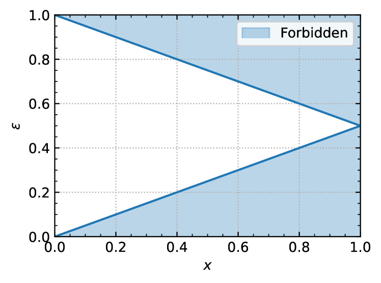
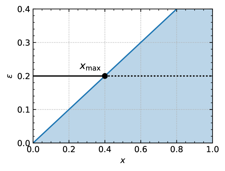
Figure 1: (Top) $(x,\epsilon)$-phase diagram of the HWM. The energy density of the HWM is contained in $0\leq\epsilon\leq 1$, and the fractional Hamming distance is $0\leq x\leq 1$. The regions shaded in blue are given by the points $(x,\epsilon)$ where $\mathcal{N}(x,\epsilon)$ is exactly zero at any given size. (Bottom) Zoomed-in detail of the $(x,\epsilon)$-phase diagram around the energy density $\epsilon=0.2$. Pairs of configurations with this energy density exist at any distance below $x_{\max}=2\epsilon$, and none above. This implies that the configurations with this energy density form one single cluster of radius $x_{\max}$.

As an example, consider the Hamming-Weight Model (HWM) defined by the Hamiltonian :

$$H(\sigma)=-\frac{1}{2}\sum_{i=1}^{N}(\sigma_{i}-1).$$ (22)

This is a non-disordered Hamiltonian and $\mathcal{N}(x,\epsilon)$ can be computed directly. Note that the triangle inequality for the Hamming distance implies that unless we have that $x/2\leq\min(\epsilon,1-\epsilon)$, then $\mathcal{N}(x,\epsilon)=0$. Assuming this inequality to hold, then

$$\mathcal{N}(x,\epsilon) =\binom{N}{\epsilon N}\binom{\epsilon N}{\frac{1}{2}xN}\binom{(1-\epsilon)N}{\frac{1}{2}xN}$$

$$=\exp\Big{\{}N\Big{[}S(\epsilon)+\epsilon S\Big{(}\frac{x}{2\epsilon}\Big{)}+$$

$$\hskip 28.45274pt+(1-\epsilon)S\Big{(}\frac{x}{2(1-\epsilon)}\Big{)}\Big{]}+o(N)\Big{\}},$$ (23)

where we have used Stirling’s approximation to show that for $0\leq p\leq 1$ one has $\binom{N}{pN}=\exp(NS(p)+o(N))$ where $S(p)\equiv-p\ln(p)-(1-p)\ln(1-p)$ is the binary Shannon entropy.

Note that in this case the $\mathcal{O}(N)$ prefactor $\Phi_{x,\epsilon}$ at the exponent is

$$\Phi_{x,\epsilon} =\lim_{N\rightarrow\infty}\frac{1}{N}\ln\mathcal{N}(x,\epsilon)$$

$$=S(\epsilon)+\epsilon S\Big{(}\frac{x}{2\epsilon}\Big{)}+(1-\epsilon)S\Big{(}\frac{x}{2(1-\epsilon)}\Big{)},$$ (24)

which is never negative since $0\leq S(p)\leq\ln 2$. Notice that even though the existence of values $x,\,\epsilon$ where $\mathcal{N}(x,\,\epsilon)=0$ does mean that there are forbidden regions in the $(x,\,\epsilon)$-phase diagram of this model, the presence of these regions does not entail clustering. This is because for any given value of $\epsilon$, the forbidden region starts at some $x_{\max}>0$ and then extends all the way to $x=1$. This implies that the configurations with energy $\epsilon N$ cannot exist at a separation larger than $x_{\max}$ but appear at all distances below that, i.e. they form one single cluster of radius $x_{\max}$. Therefore the HWM does not exhibit clustering (see Fig. 1).

V.2 The Randomly-Permuted Hamming-Weight Model

The Randomly-Permuted Hamming-Weight Model (RPHWM) is a disordered system obtained by taking the HWM and giving a random permutation to the configurations, while keeping their original energies fixed. Formally, for a fixed number of spins $N$ one samples a random element $\pi\in S_{2^{N}}$ of the permutation group over $2^{N}$ objects, uniformly at random. Then defines the energy $E_{\sigma}$ of a given spin configuration $\sigma\in\{\pm 1\}^{N}$ as $E_{\sigma}\equiv\lVert\pi(\sigma)\lVert$ where $\lVert\cdot\lVert$ is the Hamming weight norm. This model was introduced in Farhi et al. (2010).

Sampling the disorder ensemble of the RPHWM can be recast as a process of extraction from an urn without replacement, where the $2^{N}$ spin configurations are given some canonical (e.g. lexicographic) ordering $S^{(1)},\ldots,S^{(2^{N})}$, the urn contains all the possible values of the energies of the HWM with their multiplicities. These energies are randomly assigned to the configurations by extracting them sequentially from the urn, the first energy going to the configuration $S^{(1)}$, the second to $S^{(2)}$ and so on. Following this equivalent reformulation, then one can easily compute

$$\langle\mathcal{N}(x,\epsilon)\rangle =2^{N}\binom{N}{xN}\frac{1}{2^{N}}\binom{N}{\epsilon N}\frac{1}{2^{N}-1}\Big{[}\binom{N}{\epsilon N}-1\Big{]}$$

$$=\frac{1}{2^{N}-1}\binom{N}{xN}\binom{N}{\epsilon N}^{2}-\frac{1}{2^{N}-1}\binom{N}{xN}\binom{N}{\epsilon N}$$

$$\sim\exp\Big{[}N\Big{(}-\ln(2)+S(x)+2S(\epsilon)\Big{)}+o(N)\Big{]}.$$ (25)

Now we have that

$$\Phi_{x,\epsilon}=-\ln(2)+S(x)+2S(\epsilon)$$ (26)

is negative iff

$$S(\epsilon)<\frac{\ln(2)-S(x)}{2}.$$ (27)

This inequality can be solved numerically to obtain a plot of the forbidden regions in the $(x,\epsilon)$-phase diagram of the RPHWM (see Fig. 2). Setting $S(x)=0$ we obtain that clustering begins at energy densities $\epsilon$ that satisfy $S(\epsilon)<\ln(2)/2$ which for low-energy states happens around $\epsilon\approx 0.11$.

Notice, moreover, that the clusters will typically include only a subexponential number of states (their diameter being zero in fractional Hamming distance ) and therefore most of the spin variables will be frozen: starting from a state in a cluster, the flipping any such variable will necessarily move you out of the cluster. The presence of an extensive number of frozen variables in the set of solutions has been proposed as the reason behind the hardness of constraint satisfaction problems over random structures Zdeborová and Krzakala (2007); Semerjian (2008); Achlioptas and Ricci-Tersenghi (2006). Here we do not attempt to develop a formal connection between frozen variables and the algorithmic hardness our model, but leave such considerations for future works.

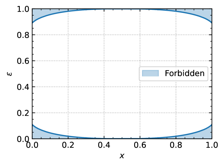
Figure 2: (Top) $(x,\epsilon)$-phase diagram of the RPHWM. The regions shaded in blue are given by the points $(x,\epsilon)$ where $\mathcal{N}(x,\epsilon)$ goes to zero in the thermodynamic limit. (Bottom) Zoomed-in detail of the $(x,\epsilon)$-phase diagram around the energy density $\epsilon=0.05$. Pairs of configurations with this energy density cannot exist at a distance smaller than $x_{\min}$ or larger than $x_{\max}$. Thus, $x_{\min}$ can be interpreted as the smallest separation between the clusters, and each cluster has zero diameter (both in fractional Hamming distance).

V.3 The Linearly-Scrambled Hamming-Weight Model

Let us define how one generates the energies of the states in a disorder realization of the Linearly-Scrambled Hamming-Weight Model (LSHWM). This is more easily described by passing to the binary representation of the spin configurations, i.e. by defining the variables $x_{i}\equiv(1-\sigma_{i})/2$ so that each spin configuration $(\sigma_{1},\ldots,\sigma_{N})\in\{\pm 1\}^{N}$ is mapped to a binary string $(x_{1},\ldots,\,x_{N})\in\mathbb{F}_{2}^{\,N}$ (see Eq. (12)). In order to generate a disorder realization of the LSHWM for a system of $N$ spins, one samples $N^{2}$ numbers $a_{ij}\in\{0,1\}$ with $1\leq i,j\leq N$ according to the symmetric probability distribution $\operatorname{Pr}[a=0]=\operatorname{Pr}[a=1]=1/2$, and defines the “scrambling matrix” $\mathbf{S}\in\mathbb{F}_{2}^{\,N\times N}$ by using the $\{a_{ij}\}$ as its entries: $\mathbf{S}_{ij}=a_{ij}$. Then every string $X=(x_{1},\ldots,x_{N})$, taken as a column vector in $\mathbb{F}^{N}_{2}$, is mapped to some new string $X^{\prime}\in\mathbb{F}_{2}^{\,N}$ according to the rule

$$\begin{bmatrix}x^{\prime}_{1}\\ \vdots\\ x^{\prime}_{N}\end{bmatrix}=\mathbf{S}\begin{bmatrix}x_{1}\\ \vdots\\ x_{N}\end{bmatrix},$$ (28)

(where matrix-vector multiplication is defined in $\mathbb{F}_{2}$) and then we define the energy $E_{\sigma}$ (that is, the energy of the spin configuration $\sigma$ represented by the binary string $X$) to be the Hamming weight of the vector $X^{\prime}$.

In the Appendix we compute, for $x,\,\epsilon>0$, the probability

$$\operatorname{Pr}\Big{[}E_{\sigma}=\epsilon N,E_{\tau}=\epsilon N\Big{]}\equiv P_{\epsilon}=2^{-2N}\binom{N}{\epsilon N}^{\!2}$$ (29)

for two configurations $\sigma,\,\tau\in\{\pm 1\}^{N}$, neither of which is the “all-spins-up” configuration (represented by the zero vector in $\mathbb{F}_{2}^{N}$, for which a positive energy density is forbidden by linearity). Then it becomes easy to show that

$$\left<\mathcal{N}(x,\epsilon)\right> =\sum_{\sigma,\tau}\delta\Big{(}d_{\sigma,\tau}-xN\Big{)}\operatorname{Pr}\Big{[}E_{\sigma}=\epsilon N,E_{\tau}=\epsilon N\Big{]}$$

$$=\sum_{\sigma\neq 0}\sum_{\tau\neq 0}\delta\Big{(}d_{\sigma,\tau}-xN\Big{)}P_{\epsilon}$$

$$=(2^{N}-1)\Big{[}\binom{N}{xN}-1\Big{]}P_{\epsilon}$$

$$\sim 2^{N}\binom{N}{xN}P_{\epsilon}$$

$$=\exp\Big{[}N\Big{(}-\ln(2)+2S(\epsilon)+S(x)\Big{)}+o(N)\Big{]}$$ (30)

therefore

$$\Phi_{x,\epsilon}=2S(\epsilon)+S(x)-\ln(2),$$ (31)

which is negative if and only if

$$S(\epsilon)<\frac{\ln(2)-S(x)}{2},$$ (32)

exactly as in the RPHWM. Therefore their clustering phase diagrams are the same.

Note that unlike the previous case, the particular ensemble of scrambling matrices used here includes non-invertible matrices and, as a consequence, the uniqueness of the ground state of the model is not guaranteed. However, provided the typical rank of the scrambling matrix scales like $\mathcal{O}(N)$, then the fraction of ground states $2^{N-\operatorname{rank}(\mathbf{S})}/2^{N}$ in the system is exponentially decaying with $N$, so these cannot be easily found just by e.g. a polynomial number of random guesses. We refer to Appendix A where we summarize the results from known literature that show that in the large-$N$ limit the typical nullity of our scrambling matrices converges to a finite value, so that their typical rank must be $\mathcal{O}(N)$ by the rank-nullity theorem.

VI Conclusion

In this work we have presented two main results. First, we have proposed a novel way of randomly generating instances of disordered Ising Hamiltonians with unique planted ground states by casting the public key of the McEliece cryptographic protocol as an interacting system of Ising spins. The algorithmic hardness of finding the ground state of the resulting Hamiltonians is equivalent to breaking the associated McEliece cryptosystem by only knowing its public key, while the private key allows the party who knows it to recover the planted ground state.

Secondly, in order to build some physical intuition as to the reason why our Hamiltonian model is hard to optimize beyond (plausible but unproven) cryptographic assumptions, we have studied the effect of random energy-scrambling on easy energy landscapes, following the notion that in the McEliece cryptosystem the public and the private keys are connected through random permutations. We have shown in simplified settings that even if the energy landscape of the Hamiltonian induced by a private key has an easy-to-find ground state, then the energy-scrambling can introduce the phenomenon known as “clustering” into the energy landscape of the Hamiltonian induced by the public key. The clustering phenomenon is known for being an obstacle to local stochastic search algorithms.

VII Acknowledgments

S.M and G.M are KBR employee working under the Prime Contract No. 80ARC020D0010 with the NASA Ames Research Center. All the authors acknowledge funding from DARPA under NASA-DARPA SAA2-403688. The United States Government retains, and by accepting the article for publication, the publisher acknowledges that the United States Government retains, a nonexclusive, paid-up, irrevocable, worldwide license to publish or reproduce the published form of this work, or allow others to do so, for United States Government purposes.

Appendix A Typical Kernel Size For Random Matrices

The probability $\mathcal{P}(\alpha)$ of a given random matrix $\mathbf{S}\in\mathbb{F}_{2}^{\,k\times k}$ having a rank ${\rm rank}(\mathbf{S})=k-\alpha$ in the limit of $k\to\infty$ can be expressed as Cooper (2000):

$$\mathcal{P}(\alpha)=2^{-\alpha^{2}}\frac{\prod_{j=\alpha+1}^{\infty}\left(1-2^{-j}\right)}{\prod_{j=1}^{\alpha}\left(1-2^{-j}\right)},$$ (33)

where we used the convention that $\prod_{j=1}^{0}(1-2^{-j})=1$. For instance, the probability of randomly sample a non-singular matrix is then $\mathcal{P}(\alpha=0)\approx 0.288788$. As shown in Fig. 3 and Table 1, $\mathcal{P}(\alpha)$ quickly goes to zero:

Matrix Rank [$k-\alpha$]	$\mathcal{P}(\alpha)$
0	0.288788
1	0.577576
2	0.12835
3	$5.239\cdot 10^{-3}$
4	$4.657\cdot 10^{-5}$
5	$9.691\cdot 10^{-8}$
6	$4.884\cdot 10^{-11}$

Table 1: Distribution of the rank or random matrices extracted from $\mathbb{F}_{2}^{\,k\times k}$, in the limit of $k\to\infty$.

with the number of elements in the kernel space having an average of $\left\langle 2^{\alpha}\right\rangle=2$ and variance ${\rm Var}[2^{\alpha}]=1$.

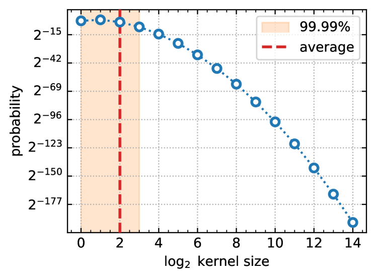
Figure 3: Distribution of the size of the kernel of random matrices extracted from $\mathbb{F}_{2}^{\,k\times k}$, in the limit of $k\to\infty$. The shaded area correspond to the $99.99\%$ of the distribution, while the dashed line corresponds to its average.

Appendix B Proof of the linear scrambling

In this appendix we will compute the probability

$$\operatorname{Pr}\Big{[}E_{x}=\epsilon N,E_{y}=\epsilon N\Big{]}$$

for the LSHWM to assign the energy value $\epsilon N$ simultaneously to two states $x\neq y\in\{0,1\}^{N}$, for $\epsilon>0$. Clearly by linearity we have that if $\epsilon>0$ and either of these states is the zero vector, then this probability must be zero. So in the following we will assume that neither of $x,y$ is zero. Given a realization of disorder $\mathbf{S}=\{a_{ij}\}$ (i.e. a random matrix of the LSHWM ensemble), the energies of $x,y$ are

$$E_{x} =\sum_{j=1}^{N}\Big{[}\sum_{k=1}^{N}a_{jk}x_{k}\pmod{2}\Big{]}\equiv\sum_{j=1}^{N}E^{(j)}_{x},$$

$$E_{y} =\sum_{j=1}^{N}\Big{[}\sum_{k=1}^{N}a_{jk}y_{k}\pmod{2}\Big{]}\equiv\sum_{j=1}^{N}E^{(j)}_{y}.$$

We partition the set $[N]\equiv\{1,2,\ldots,N\}$ as

$$[N]= \{k\mid x_{k}=y_{k}=0\}\cup\{k\mid x_{k}=y_{k}=1\}$$

$$\cup\{k\mid x_{k}=0,y_{k}=1\}\cup\{k\mid x_{k}=1,y_{k}=0\}$$

$$\equiv (00)\cup(11)\cup(01)\cup(10)$$

and coarse-grain the disordered degrees of freedoms $\{a_{jk}\}$ in $2^{\alpha N}$ “macrostates” $\mathcal{S}\in\{0,1\}^{\alpha N}$ where each of the $\alpha N$ coarse-grained binary variables $\mathcal{S}_{\gamma}^{(j)}$ of $\mathcal{S}$ are functions of the matrix entries $\{a_{jk}\}_{jk}$. For each $j=1,\ldots,N$ we define

$$\mathcal{S}_{\gamma}^{(j)}\equiv\sum_{k\in\gamma}a_{jk}\pmod{2},\quad\text{for $\gamma\in\Big{\{}(00),(01),(10),(11)\Big{\}}$}$$

so that

$$\mathcal{S}=\Big{(}\;\Big{\{}\mathcal{S}^{(j)}_{00}\Big{\}}_{j=1}^{N},\Big{\{}\mathcal{S}^{(j)}_{01}\Big{\}}_{j=1}^{N},\Big{\{}\mathcal{S}^{(j)}_{10}\Big{\}}_{j=1}^{N},\Big{\{}\mathcal{S}^{(j)}_{11}\Big{\}}_{j=1}^{N}\;\Big{)}.$$

The integer $\alpha\in\{2,3,4\}$ will depend on the states $x,y$ (specifically, whether or not there exist indices $k$ where $x_{k}=y_{k}=0$ so that the set $(00)$ is nonempty, and analogously for $(01),(10)$ and $(11)$), and we will distinguish cases. A specific choice of values for the disordered variables $\{a_{jk}\}_{jk}$ will induce a unique macrostate, i.e. an assignment of Boolean values to all variables $\{\mathcal{S}_{\gamma}^{(j)}\}_{j,\gamma}$, while a specific choice of values for $\{\mathcal{S}_{\gamma}^{(j)}\}_{j,\gamma}$ will be compatible with multiple “microstates” $\{a_{jk}\}_{jk}$. Note that the variables $a_{ij}$ involved in the definitions of the $\mathcal{S}_{\gamma}^{(j)}$ for different $\gamma$, are all independent.

Then the energies of the states $x,y$ we can be written as a function of the macrostate variables:

$$E_{x} =\sum_{j=1}^{N}E_{x}^{(j)}=\sum_{j=1}^{N}\Big{[}\mathcal{S}_{11}^{(j)}+\mathcal{S}_{10}^{(j)}\pmod{2}\Big{]}$$

$$E_{y} =\sum_{j=1}^{N}E_{y}^{(j)}=\sum_{j=1}^{N}\Big{[}\mathcal{S}_{11}^{(j)}+\mathcal{S}_{01}^{(j)}\pmod{2}\Big{]}$$

Observe in particular that the energies do not depend on the macrostate variables $\mathcal{S}_{00}^{(j)}$. In order to compute the probability of having $E_{x}=E_{y}=\epsilon N$ we need to count how many ways we can choose values for the macrostate variables that will give us this energy value for both $E_{x}$ and $E_{y}$, and then weight each choice by its appropriate probability induced by the distribution of the microscopic degrees of freedom $\{a_{jk}\}_{jk}$ compatible with that choice. We distinguish the following three main cases, summarized in Fig. 4.

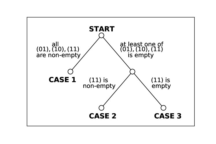
Figure 4: Logical flowchart of the three main cases for the calculation of the probability $\operatorname{Pr}\Big{[}E_{x}=\epsilon N,E_{y}=\epsilon N\Big{]}$ in the LSHWM.

• Case 1: the three subsets $\gamma=(11),(01),(10)$ are non-empty. Let us fix a vector $\mathcal{S}_{11}=(\mathcal{S}_{11}^{(1)},\ldots,\mathcal{S}_{11}^{(N)})\in\{0,1\}^{N}$. In order to have $E_{x}=\epsilon N$ we need to have $\epsilon N$ indices $0\leq j\leq N$ where $E^{(j)}_{x}=1$. This fixes the values of $\mathcal{S}^{(j)}_{10}$ since we need to have $\epsilon N$ indices where $\mathcal{S}^{(j)}_{10}=1-\mathcal{S}^{(j)}_{11}$ and the other $(1-\epsilon)N$ must be $\mathcal{S}^{(j)}_{11}=\mathcal{S}^{(j)}_{10}$. Analogously we need to choose $\epsilon N$ values of $j$ where $E_{y}^{(j)}=1$. These can be chosen independently from the choices of $E_{x}^{(j)}$. This fixes the values $\mathcal{S}^{(j)}_{10}$.

  • Case 1.A: the subset $(00)$ is non-empty Then $\alpha=4$ and we have the $N$ degrees of freedom in $\mathcal{S}^{(j)}_{00}$ that are completely free and do not affect the energies at all. So for a fixed $\mathcal{S}_{11}=(\mathcal{S}_{11}^{(1)},\ldots,\mathcal{S}_{11}^{(N)})\in\{0,1\}^{N}$ we have

    $$2^{N}\binom{N}{\epsilon N}^{2}$$

    choices to achieve that $E_{x}=E_{y}=\epsilon N$. Which means that at the level of the macrostates $\mathcal{S}$, the number $n_{M}$ of choices that give $E_{x}=E_{y}=\epsilon N$ is

    $$n_{M}=2^{2N}\binom{N}{\epsilon N}^{2}$$

    What is left to do is to compute the entropies of the macrostates. A given value $\mathcal{S}_{\gamma}^{(j)}$ is compatible with half of the microstates of the variables $a_{ij}$ that appear in its definition, and all of these choices are independent for different $j$ and $\gamma$, so we get (remember that here $\alpha=4$)

    $$2^{-\alpha N}\Big{[}2^{N}\Big{]}^{N}2^{2N}\binom{N}{\epsilon N}^{2}=2^{N^{2}}2^{-2N}\binom{N}{\epsilon N}^{2}$$

    out of a total of $2^{N^{2}}$ microstates, so the probability we seek is given by

    $$\operatorname{Pr}\Big{[}E_{\sigma}=\epsilon N,E_{\tau}=\epsilon N\Big{]}=2^{-2N}\binom{N}{\epsilon N}^{2}\equiv P_{\epsilon}$$

  • Case 1.B: the subset $(00)$ is empty In this case $\alpha=3$ and we have already fixed all macrostate variables. By an analogous calculation to the Case 1.A we have

    $$n_{M}=2^{N}\binom{N}{\epsilon N}^{2}$$

    choices for the macrostate variables compatible with $E_{x}=E_{y}=\epsilon N$. In the language of the microstates, we have

    $$2^{-\alpha N}\Big{[}2^{N}\Big{]}^{N}2^{N}\binom{N}{\epsilon N}^{2}=2^{N^{2}}2^{-2N}\binom{N}{\epsilon N}^{2}$$

    choices out of $2^{N^{2}}$ total microstates. This gives the same value $P_{\epsilon}$ for the probability, as before.

• Case 2: $(11)$ is non-empty, and at least one between $(01),(10)$ is empty. Notice that in this case we must have that exactly one between $(01),(10)$ is empty (if both are empty then $x=y$, a possibility that we have ruled out by assumption). Since the states $x,y$ play a perfectly symmetrical role in the probability we are trying to compute we can assume without loss of generality that $(01)$ is non-empty and $(10)$ is empty. In this case, in order to have $E_{x}=\epsilon N$ we have to choose $\epsilon N$ variables $\mathcal{S}_{11}^{(j)}$ to be set to one, and all the others to zero ($\binom{N}{\epsilon N}$ choices). This fixes the vector $\mathcal{S}_{11}$. In order to obtain $E_{y}=\epsilon N$ we have to choose $\epsilon N$ variables $\mathcal{S}_{01}^{(j)}$ to be set equal to $\mathcal{S}_{01}^{(j)}=1-\mathcal{S}_{11}^{(j)}$ and the others to $\mathcal{S}_{01}^{(j)}=\mathcal{S}_{11}^{(j)}$ (another $\binom{N}{\epsilon N}$ choices). This fixes the vector $\mathcal{S}_{01}$.

  • Case 2.A: the subset $(00)$ is non-empty Then $\alpha=3$ and the proof follows Case 1.A with $n_{M}=2^{N}\binom{N}{\epsilon N}$ which leads to a probability of $P_{\epsilon}$ as before.

  • Case 2.B: the subset $(00)$ is empty Then $\alpha=2$ and the proof follows Case 2.A with $n_{M}=\binom{N}{\epsilon N}$ which leads to a probability of $P_{\epsilon}$ as before.

• Case 3: $(11)$ is empty. In this case we must have that both $(01)$ and $(10)$ are non-empty, otherwise at least one between $x$ and $y$ is the zero vector, a possibility that we have ruled out by assumption. In order to have $E_{x}=E_{y}=\epsilon N$ we have to set to one exactly $\epsilon N$ variables $\mathcal{S}_{01}^{(j)}$, and exactly $\epsilon N$ variables $\mathcal{S}_{10}^{(j)}$, independently. This gives $\binom{N}{\epsilon N}^{2}$ choices. This fixes the vectors $\mathcal{S}_{01}$ and $\mathcal{S}_{10}$.

  • Case 3.A: the subset $(11)$ is non-empty Then $\alpha=3$ and the proof follows Case 1.A with $n_{M}=2^{N}\binom{N}{\epsilon N}$ which leads to a probability of $P_{\epsilon}$ as before.

  • Case 3.B: the subset $(11)$ is empty Then $\alpha=2$ and the proof follows Case 2.A with $n_{M}=\binom{N}{\epsilon N}$ which leads to a probability of $P_{\epsilon}$ as before.

References

- Arute et al. (2019) F. Arute, K. Arya, R. Babbush, D. Bacon, J. C. Bardin, R. Barends, R. Biswas, S. Boixo, F. G. Brandao, D. A. Buell, et al., Nature 574, 505 (2019).
- Morvan et al. (2023) A. Morvan, B. Villalonga, X. Mi, S. Mandra, A. Bengtsson, P. Klimov, Z. Chen, S. Hong, C. Erickson, I. Drozdov, et al., arXiv preprint arXiv:2304.11119 (2023).
- Kim et al. (2023) Y. Kim, A. Eddins, S. Anand, K. X. Wei, E. Van Den Berg, S. Rosenblatt, H. Nayfeh, Y. Wu, M. Zaletel, K. Temme, et al., Nature 618, 500 (2023).
- Kim et al. (2021) M. Kim, S. Mandrà, D. Venturelli, and K. Jamieson, in Proceedings of the 27th Annual International Conference on Mobile Computing and Networking (2021) pp. 42–55.
- Aramon et al. (2019) M. Aramon, G. Rosenberg, E. Valiante, T. Miyazawa, H. Tamura, and H. G. Katzgraber, Frontiers in Physics 7, 48 (2019).
- Zhu et al. (2015) Z. Zhu, A. J. Ochoa, and H. G. Katzgraber, Physical review letters 115, 077201 (2015).
- Mohseni et al. (2022) N. Mohseni, P. L. McMahon, and T. Byrnes, Nature Reviews Physics 4, 363 (2022).
- Sao et al. (2019) M. Sao, H. Watanabe, Y. Musha, and A. Utsunomiya, Fujitsu Scientific and Technical Journal 55, 45 (2019).
- Traversa and Di Ventra (2015) F. L. Traversa and M. Di Ventra, IEEE transactions on neural networks and learning systems 26, 2702 (2015).
- Adleman (1994) L. M. Adleman, science 266, 1021 (1994).
- Papadimitriou and Steiglitz (1998) C. H. Papadimitriou and K. Steiglitz, Combinatorial optimization: algorithms and complexity (Courier Corporation, 1998).
- Sipser (1996) M. Sipser, ACM Sigact News 27, 27 (1996).
- Biere et al. (2009) A. Biere, M. Heule, and H. van Maaren, Handbook of satisfiability, Vol. 185 (IOS press, 2009).
- Qu and Potkonjak (1999) G. Qu and M. Potkonjak, in International Workshop on Information Hiding (Springer, 1999) pp. 348–367.
- Barthel et al. (2002) W. Barthel, A. K. Hartmann, M. Leone, F. Ricci-Tersenghi, M. Weigt, and R. Zecchina, Physical review letters 88, 188701 (2002).
- Krzakala and Zdeborová (2009) F. Krzakala and L. Zdeborová, Physical review letters 102, 238701 (2009).
- Zdeborová and Krzakala (2011) L. Zdeborová and F. Krzakala, SIAM Journal on Discrete Mathematics 25, 750 (2011).
- Krzakala et al. (2012) F. Krzakala, M. Mézard, and L. Zdeborová, Journal on Satisfiability, Boolean Modeling and Computation 8, 149 (2012).
- Sicuro and Zdeborová (2021) G. Sicuro and L. Zdeborová, Journal of Physics A: Mathematical and Theoretical 54, 175002 (2021).
- Mézard et al. (2002) M. Mézard, G. Parisi, and R. Zecchina, Science 297, 812 (2002).
- Zdeborová and Krzakala (2007) L. Zdeborová and F. Krzakala, Physical Review E 76, 031131 (2007).
- Ricci-Tersenghi et al. (2019) F. Ricci-Tersenghi, G. Semerjian, and L. Zdeborová, Physical Review E 99, 042109 (2019).
- Semerjian et al. (2020) G. Semerjian, G. Sicuro, and L. Zdeborová, Physical Review E 102, 022304 (2020).
- Zdeborová and Mézard (2008) L. Zdeborová and M. Mézard, Journal of Statistical Mechanics: Theory and Experiment 2008, P12004 (2008).
- Denchev et al. (2016) V. S. Denchev, S. Boixo, S. V. Isakov, N. Ding, R. Babbush, V. Smelyanskiy, J. Martinis, and H. Neven, Physical Review X 6, 031015 (2016).
- Hen et al. (2015) I. Hen, J. Job, T. Albash, T. F. Rønnow, M. Troyer, and D. A. Lidar, Physical Review A 92, 042325 (2015).
- Wang et al. (2017) W. Wang, S. Mandrà, and H. G. Katzgraber, Physical Review E 96, 023312 (2017).
- Hamze et al. (2018) F. Hamze, D. C. Jacob, A. J. Ochoa, D. Perera, W. Wang, and H. G. Katzgraber, Physical Review E 97, 043303 (2018).
- Perera et al. (2020) D. Perera, F. Hamze, J. Raymond, M. Weigel, and H. G. Katzgraber, Physical Review E 101, 023316 (2020).
- Hen (2019) I. Hen, Physical Review Applied 12, 011003 (2019).
- Hamze et al. (2020) F. Hamze, J. Raymond, C. A. Pattison, K. Biswas, and H. G. Katzgraber, Physical Review E 101, 052102 (2020).
- Thouless et al. (1977) D. J. Thouless, P. W. Anderson, and R. G. Palmer, Philosophical Magazine 35, 593 (1977).
- King et al. (2019) J. King, S. Yarkoni, J. Raymond, I. Ozfidan, A. D. King, M. M. Nevisi, J. P. Hilton, and C. C. McGeoch, Journal of the Physical Society of Japan 88, 061007 (2019).
- Mandra et al. (2016) S. Mandra, Z. Zhu, W. Wang, A. Perdomo-Ortiz, and H. G. Katzgraber, Physical Review A 94, 022337 (2016).
- Mandra et al. (2017) S. Mandra, H. G. Katzgraber, and C. Thomas, Quantum Science and Technology 2, 038501 (2017).
- Mandra et al. (2019) S. Mandra, B. Villalonga, S. Boixo, H. Katzgraber, and E. Rieffel, in APS March Meeting Abstracts, Vol. 2019 (2019) pp. C42–013.
- Mandra and Katzgraber (2018) S. Mandra and H. G. Katzgraber, Quantum Science and Technology 3, 04LT01 (2018).
- Merkle and Hellman (1978) R. Merkle and M. Hellman, IEEE transactions on Information Theory 24, 525 (1978).
- Papadimitriou (2003) C. H. Papadimitriou, in Encyclopedia of computer science (2003) pp. 260–265.
- Shamir (1982) A. Shamir, in 23rd Annual Symposium on Foundations of Computer Science (sfcs 1982) (IEEE, 1982) pp. 145–152.
- Pirnay et al. (2022) N. Pirnay, V. Ulitzsch, F. Wilde, J. Eisert, and J.-P. Seifert, arXiv preprint arXiv:2212.08678 (2022).
- Szegedy (2022) M. Szegedy, arXiv preprint arXiv:2212.12572 (2022).
- Shor (1999) P. W. Shor, SIAM review 41, 303 (1999).
- McEliece (1978) R. J. McEliece, Coding Thv 4244, 114 (1978).
- Bernstein et al. (2008) D. J. Bernstein, T. Lange, and C. Peters, in Post-Quantum Cryptography: Second International Workshop, PQCrypto 2008 Cincinnati, OH, USA, October 17-19, 2008 Proceedings 2 (Springer, 2008) pp. 31–46.
- Dinh et al. (2011) H. Dinh, C. Moore, and A. Russell, in Advances in Cryptology–CRYPTO 2011: 31st Annual Cryptology Conference, Santa Barbara, CA, USA, August 14-18, 2011. Proceedings 31 (Springer, 2011) pp. 761–779.
- (47) NIST, Post-quantum cryptography (PQC), https://csrc.nist.gov/projects/post-quantum-cryptography/round-3-submissions.
- Mézard et al. (2005) M. Mézard, T. Mora, and R. Zecchina, Phys. Rev. Lett. 94, 197205 (2005).
- Achlioptas and Ricci-Tersenghi (2006) D. Achlioptas and F. Ricci-Tersenghi, in Proceedings of the Thirty-Eighth Annual ACM Symposium on Theory of Computing, STOC ’06 (Association for Computing Machinery, New York, NY, USA, 2006) p. 130–139.
- Coja-Oghlan et al. (2017) A. Coja-Oghlan, A. Haqshenas, and S. Hetterich, SIAM Journal on Discrete Mathematics 31, 1160 (2017), https://doi.org/10.1137/16M1084158 .
- Gamarnik (2021) D. Gamarnik, Proceedings of the National Academy of Sciences 118, e2108492118 (2021), https://www.pnas.org/doi/pdf/10.1073/pnas.2108492118 .
- Angelini and Ricci-Tersenghi (2023) M. C. Angelini and F. Ricci-Tersenghi, Phys. Rev. X 13, 021011 (2023).
- Note (1) By changing into the binary representation of the spin configuration through the defining , then is the Hamming weight of the associated binary string .
- Farhi et al. (2010) E. Farhi, J. Goldstone, D. Gosset, S. Gutmann, and P. Shor, (2010), arXiv:1010.0009 .
- Note (2) This is observed also in e.g. the Random Energy Model, where .
- Zdeborová and Krzakala (2007) L. Zdeborová and F. Krzakala, Phys. Rev. E 76, 031131 (2007).
- Semerjian (2008) G. Semerjian, Journal of Statistical Physics 130, 251 (2008).
- Cooper (2000) C. Cooper, Random Structures & Algorithms 17, 197 (2000).