ShapFuzz: Efficient Fuzzing via Shapley-Guided Byte Selection

Abstract

Mutation-based fuzzing is a popular and effective method for bug exposure and discovery of unseen code in programs. However, only a few studies have focused on quantifying the importance of input bytes. The importance of each input byte is determined by its contribution degree in discovering new code. Previous work often focused on obtaining the relationship between input bytes and path constraints, ignoring the fact that not all constraint-related bytes can discover new code. In this paper, we conduct Shapley analysis to understand the effect of byte positions on fuzzing performance, and find that some byte positions contribute more than others and this property often holds across different seeds. Based on this observation, we propose a novel solution, called ShapFuzz, to guide byte selection and mutation in fuzzing processes. Specifically, ShapFuzz updates Shapley values (importance) of bytes when each input is tested during fuzzing with a low overhead. It utilizes contextual multi-armed bandit algorithm to make a trade off between mutating high Shapley value bytes and low-frequently chosen bytes. We implement a prototype of this solution based on AFL++, i.e., ShapFuzz, and evaluate it against ten state-of-the-art fuzzers, including five byte-scheduling fuzzers and five commonly used fuzzers. Compared to byte-scheduling fuzzers, ShapFuzz discovers more edges. It also exposes more bugs than the best baseline on three different sets of initial seeds. ShapFuzz exposes 20 more bugs than the best commonly used fuzzers, and discovers 6 more CVEs than the baseline on MAGMA. Furthermore, ShapFuzz discovers 11 new bugs on the latest versions of 6 widely used programs, and 3 bugs of them are confirmed by vendors.

I Introduction

Mutation-based fuzzing is widely used to detect software vulnerabilities among both academic and industrial practitioners [44]. In general, to mutate an input, there are two core choices to make: which bytes to mutate (byte selection) and what values to use (value update). To mutate bytes, state-of-the-art solutions often rely on extra analysis to recognize the bytes related to path constraints. The first category of solutions utilizes taint analysis to track constraint-related bytes. TaintScope [35], Dowser [13] and Angora [6] are examples of the first category. The second category indirectly infers the dependence between bytes and constraints. Members of this category include GREYONE [12], REDQUEEN [1], ProFuzzer [37] and PATA [22]. The third category finds where to mutate by extracting information from historical data. Examples are NEUZZ [32], MTFuzz [31] and EMS [26].

While mutating constraint-related bytes indeed improves the efficiency of code discovery, not all constraint-related bytes are able to discover new code. In fact, our experiments show that only 18% of constraint-related bytes can be mutated to successfully discover new areas (Section IV-E). For some target programs, this ratio is even less than 3%. However, existing solutions treat all constraint-related bytes equally, wasting time and energy on the ones that cannot discover new code. Moreover, the extra analysis stage required by existing solutions is often time-consuming due to its byte-by-byte investigation [12, 37, 22]. For deep learning-based fuzzers [32, 31], the extra stage may even fail the process of fuzzing because a large input size will cause out-of-memory errors when building models.

To solve these problems, our key idea is to quantify the importance of constraint-related bytes (i.e., the degree to which a byte contributes to the discovery of new code), without going through the extra analysis stage. Basically, the discovery of new edges is due to the cooperation of certain bytes, or more precisely, their cooperative mutations. This motivates us to take the perspective of Cooperative Game Theory [30] and study the byte scheduling part of fuzzing as a process of Shapley analysis [24]. Shapley analysis is widely used to quantify the contribution of each player to the result. By quantifying the importance of input bytes, we can find the bytes that are more likely to discover new code and do more mutations on those bytes. This solution does not require going through an extra analysis stage to obtain the importance because the Shapley analysis can be integrated into the process of mutation.

We have conducted a set of fuzzing experiments and performed Shapley analysis to determine the contribution of each byte to discovering new code. Interestingly, the analysis demonstrated that (1) the discovery of new code largely depends on a small portion of byte positions, and (2) the mutation of the same byte positions can repeatedly discover new code. We observe that these two findings match the nature of program logic. Specifically, some input bytes are repeatedly utilized in the path constraints that prevent fuzzing from discovering code. Our experiments also demonstrated that 86% of constraint-related bytes are related to multiple CMP instructions used in path constraints (Section II). In other words, repetitive mutation of high-importance bytes (the small portion) can efficiently solve constraints in different paths.

While Shapley analysis sounds promising in guiding byte mutations, the full Shapley analysis of a byte requires that all the possible inputs related to that byte to be generated and tested. Then, no new inputs can be generated for the byte after the full Shapley analysis, making the Shapley values useless for guiding fuzzing. Therefore, we propose to utilize temporary Shapley values calculated by incomplete Shapley analysis to guide fuzzing. The aforementioned empirical observation implies that this is feasible. The bytes that temporarily show high Shapley values are still likely related to multiple unseen path constraints.

In this paper, we propose ShapFuzz to boost the efficiency of byte selection based on Shapley analysis. Specifically, we formulate the solution to byte selection as a Shapley analysis across multiple seed inputs. To reduce the overhead of calculating Shapley values, we classify seeds into different families and share Shapley values in each family, and further transform the Shapley value calculation into a form that can be gradually updated by each seed input. We further utilize contextual multi-armed bandit (CMAB) to maximize the efficiency of fuzzing when we use temporary Shapley values. On the one hand, high Shapley value bytes might not be useful in some situations, e.g., when all related constraints of a byte have been explored. On the other hand, to update the temporary Shapley values, we need to provide opportunities to low-frequently chosen bytes. Therefore, CMAB makes a trade-off between mutating high Shapley value bytes and low-frequently chosen ones.

We implement a prototype ShapFuzz based on AFL++ [10]. We evaluate it on two third-party benchmarks, including 1) UNIFUZZ [21], which contains real-world programs, and 2) MAGMA [14], which provides a series of real-world programs with known bugs. We compare their performance with 10 widely-used fuzzers, including 5 byte-scheduling fuzzers (GreyOne [12], ProFuzzer [37], Angora [6], PreFuzz [36] and NEUZZ [32]) and 5 commonly used fuzzers (AFL++ [10], MOPT [25], AFLFast [3], FairFuzz [18] and AFL [40]). Compared with byte-scheduling fuzzers, when all initial seeds are given, ShapFuzz discovers 4170 more edges and exposes 19 more bugs than the best baseline. In addition, when given two initial seed sets with lengths less than 10,000 and 1,000 bytes, ShapFuzz is still able to discover the majority of edges and expose most of the bugs. ShapFuzz discovers 20 to 68 more bugs than what the five commonly used fuzzers do, and exposes six more CVEs than what the best of the five fuzzers does. Furthermore, ShapFuzz discovers 11 new bugs, 3 of which are confirmed by vendors.

We summarize our main contributions as follows.

• Based on Shapley analysis, we perform empirical experiments to study the contributions of bytes in terms of code discovery. The results indicate that the repeated mutation of a small portion of positions can improve the efficiency of code discovery. We ascertain that the main derivative of the Shapley results is that a byte may be related to multiple path constraints.

• We formalize byte selection as Shapley analysis and transform the calculation of Shapley values into a form that can be updated gradually during fuzzing. We propose ShapFuzz, which uses Shapley values to guide the byte selection process. It presents a contextual multi-armed bandit approach to optimize Shapley-guided byte selection.

• We implement ShapFuzz based on AFL++, and evaluate it on UNIFUZZ and MAGMA platforms. The results indicate that ShapFuzz outperforms various state-of-the-art fuzzers in terms of edge coverage and bug discovery. We open source ShapFuzz at https://github.com/ShapFuzz/ShapFuzz.

II Background and Motivation

The aim of coverage-guided fuzzing is to expand the code coverage, which motivates us to study the contributions of bytes in inputs in terms of discovering new coverage. In this section, we study the contributions (or importance) of bytes in terms of code discovery.

II-A Shapley Analysis and CMAB

In this section, we introduce the concept of Shapley analysis and contextual multi-armed bandit.

II-A1 Shapley Analysis

In cooperative game theory, a coalition of players participate in a game and obtain a gain. The key question is how much each player contributes to the coalition. Many methods have been proposed to address this problem. The best-known solution to this question is the Shapley value [30], a method for distributing gain among players in a cooperative game. Specifically, the Shapley value is the weighted average of each player’s marginal contributions to all possible coalitions of players. Moreover, the Shapley value has been applied in numerous fields, such as quantifying the importance of a feature in deep learning models [11].

II-A2 CMAB

The multi-armed bandit problem is a model to study the trade-offs between exploring new knowledge and exploiting the current reliable knowledge [17]. Formally, a bandit problem consists of a set of $N$ arms. At the trial $t$, the player pulls an arm $i$ and receives a reward $r_{t}$. The goal of the player is to maximize the total reward in finite trials. However, the player can estimate the expected reward for each arm only through repeated trials. Thus, the player needs to make a trade-off between finding out the reward expectation of each arm and choosing the arm with the highest reward. The contextual bandit problem is a variant of the multi-armed bandit problem [2]. In each trial, the player is presented with side information (i.e., context) before making decision. Since the expected reward of arms may be different in different contexts, the player needs to consider the influence of context when choosing an arm.

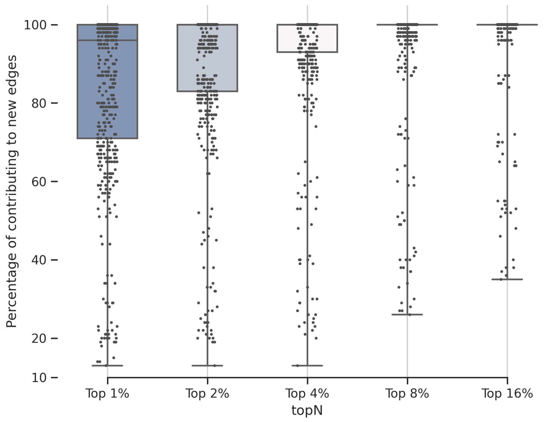
Figure 1: The boxplot of contributions of bytes. Y% of new edges are contributed by the top X% of bytes. The top X% of bytes refers to the first X% bytes with the largest Shapley values. Each dot is a seed of a program.

II-B Motivation

Since bytes are collaboratively mutated to explore code, we use the concept of Shapley value, which is a solution concept in Cooperative Game Theory, to analyze the contributions of bytes. The core idea of Shapley value is to traverse all possible combinations and calculate the average marginal contribution of a byte based on the gains of those combinations. More details are explained in Section III-A1.

II-B1 Experiments of Shapley Analysis

To calculate Shapley values of bytes in a seed, we regard the number of new edges discovered by a combination as the gain. However, a seed with length $N$ has $256^{N}$ possible combinations, which are too many to be tested. To obtain a relatively accurate Shapley value for a byte, we run fuzzing with random mutation for 48 hours for a single seed. Specifically, we use AFL++ to run fuzzing on 18 programs with a set of initial seeds for 48 hours. Each fuzzing experiment is only performed on a single initial seed of a program and we do not update the seed queue but continuously mutate the selected initial seed. The experiments are repeated six times to avoid the influence of randomness. The 18 programs, such as nm, tiff2bw, flvmeta, imginfo, infotocap, lame, mp42aac and mp3gain, include 9 different types of inputs that are elf, tiff, pdf, text, mp4, flv, wav, jpg and mp3. During fuzzing, if a mutation discovers new edges, we will recover all the subsets of related bytes and test the result. For example, if the mutation of positions $\{1,3,4\}$ discovers new edges (the gain $R$), all the subsets $\{1\}/\{3\}/\{4\}/\{1,3\}/\{1,4\}/\{3,4\}$ will be recovered, and their results will be tested. This ensures that all possible combinations related to the gain $R$ are analyzed. Finally, based on these results, we can calculate the Shapley values for positions $1$, $3$, and $4$. Notably, we remove the mutators that can change the length of a seed so that each byte does not change its relative position.

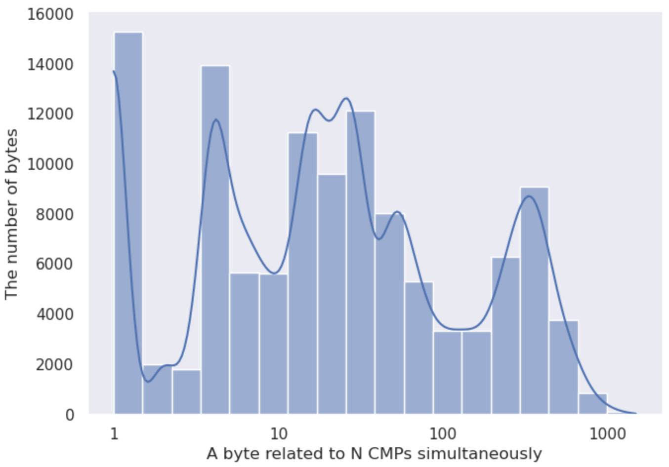
Figure 2: Statistics of the relationship between bytes and CMPs across 16 programs.

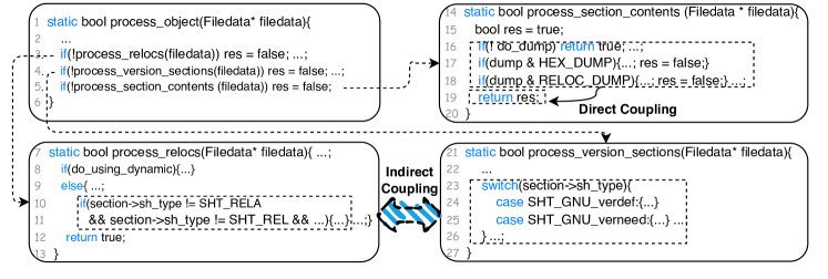
Figure 3: The reason for the results of SHAP analysis. The code is extracted from readelf.

The experiment results are shown in Figure 1, where each dot means that for a program and an initial seed, Y% of new edges are contributed by top X% bytes. The results indicate that a small portion of bytes contribute the most to discovering new edges. For example, the top 4% positions contribute to the discovery of 97.43%, 88.72%, 86.10%, 94.16%, 87.96%, and 100.00% edges on pdftotext, tcpdump, infotocap, strip, objdump, and flvmeta, respectively. On some programs, such as tiffsplit, the top 1% bytes can contribute more than 90% of new edges. This also indicates that some bytes repeatedly discover new code during fuzzing.

II-B2 Interpretability of the Shapley Results

In a program input, not all bytes pertain to path constraints. Even for the bytes related to the same path constraint, they contribute differently to solving the constraint. For instance, in the snippet $if((int)a>0xeffff)$, the mutation of the two high bytes is more likely to satisfy the condition while the mutation of the two low bytes may not be able to satisfy it. Moreover, a byte may be related to more than one path constraint, which increases the Shapley value of the byte. From the perspective of program logic, this is the result of path coupling. On the one hand, along the same execution path, the flipping of a path constraint has to consider the results of other path constraints. For example, in Figure 3, the path constraint in line 5 is defined by the function process_section_contents(), whose boolean output is determined by the constraints of lines 16, 17 and 18. Thus, input bytes related to lines 16, 17 and 18 also contribute to the solving of constraint in line 5. On the other hand, different program logics may process the same bytes of inputs. For instance, in Figure 3, both the constraints of lines 10 and 23 check the value of sh_type, which represents the types of sections in the program.

To further investigate the generality of a byte being related to multiple path constraints simultaneously, we take the CMP operator as an example and analyze the overlapping situations of related bytes among CMPs in 16 programs, including nm, tiff2bw, and so on. We use the GreyOne’s FTI [12] method to analyze the related bytes of CMP, which has the characteristic of no false positives. Specifically, given a CMP and a seed, if changing byte $i$ of the seed leads to a change in the value of CMP $j$, then byte $i$ and CMP $j$ are related. Finally, we combine the analysis results of all programs to obtain the final experimental results, as shown in Figure 2. We found that most bytes are related to multiple CMPs. For instance, 86% of bytes are related to more than two CMPs. There are 6,000 bytes that are related to 10 CMPs at the same time. This experiment shows that the sharing of related bytes between CMPs is a common phenomenon.

II-B3 Insight

Since only a small portion of bytes contribute the most to the discovery of new code, the Shapley analysis can be utilized to obtain those high-importance bytes and more energy is assigned to them during fuzzing. Because it is common that a constraint-related byte is related to multiple CMP instructions, focusing on the high-importance bytes can improve the efficiency of code discovery in unseen paths. Although this insight has been validated in the programs we tested, it is essential to acknowledge that additional validation on a broader range of programs is necessary to establish its generalizability.

III Design of ShapFuzz

Our ShapFuzz focuses on the byte mutation and quantifies the importance of byte positions. We understand the byte mutation across multiple seeds as a process of Shapley analysis and use the Shapley value to quantify the contribution of each byte. Figure 4 shows the framework of our ShapFuzz, which uses Shapley values of bytes to boost fuzzing efficiency. We treat the schedule of bytes on the seed as the cooperative game and calculate the Shapley value for each byte. To relieve the overhead of Shapley analysis, we deduce that the seeds, which are retained from the same original seed and do not change the length, belong to the same cooperative game and share the same Shapley values for bytes. Thus, we group such seeds into a family to calculate the shared Shapley values in each family.

Fuzzing efficiency can be improved by assigning more energy to the bytes with higher Shapley values. However, we need to mutate all bytes and generate all possible inputs to get an accurate Shapley Value during fuzzing. To make the trade-off between mutating high Shapley value bytes and low-frequently chosen bytes, ShapFuzz uses CMAB to build a probability distribution for optimizing this trade-off.

III-A Shapley Analysis Among Bytes

As mentioned, bytes in a seed are collaboratively mutated to discover new edges. Therefore, we formulate the process of byte mutation as a cooperative game and use Shapley value to quantify the contribution of each byte. We first formulate the mutation of one seed and then extend it to multiple seeds based on the characteristics of mutation.

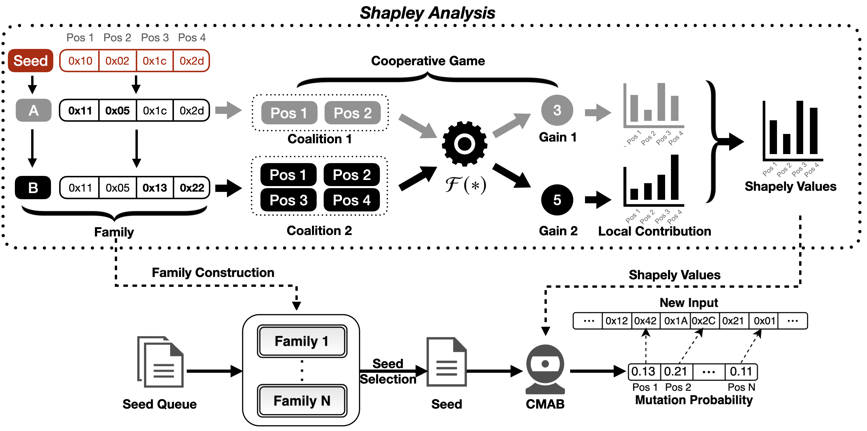
Figure 4: The Framework of ShapFuzz. It groups seeds into families, calculates Shapely values, and utilizes CMAB to optimize Shapley-guided byte mutation.

III-A1 Shapley Value

The Shapley value is a solution used in Cooperative Game Theory that fairly distributes gains among several players working in a coalition. A cooperative game is one that $N$ players form coalitions and obtain gains by a characteristic function. Shapley Value can be used to quantify the contribution of each player in a game. In the Cooperative Game Theory, the Shapley Value $\phi_{j}$ of the player $x_{j}$ to the coalition can be calculated as [30]:

$$\phi_{j}=\sum_{G\subseteq X\backslash\{x_{j}\}}\frac{|G|!(N-|G|-1)!}{N!}(\mathcal{F}(G\cup\{x_{j}\})-\mathcal{F}(G)),$$ (1)

where there are $N$ players in the game, and a coalition $G$ is formed by $m(m\leq N)$ players. $X$ is the set of all players and $X\backslash\{x_{j}\}$ is all possible coalitions of players excluding the player $x_{j}$. $|G|$ is the number of players in the set $G$. $\mathcal{F}(\ast)$ is a characteristic function that describes the gain $R$ that the coalition of players can obtain, i.e., $R=\mathcal{F}(G)$. $\mathcal{F}(G\cup\{x_{j}\})-\mathcal{F}(G)$ is the marginal contribution of the player $x_{j}$ on the coalition $G$, which describes the effect on the gain by the player $x_{j}$. In other words, the Shapley value $\phi_{j}$ is a weighted average of $x_{j}$’s marginal contributions across all possible player coalitions. In other words, the Shapley value reflects the importance of the player $x_{j}$ in the game.

Coverage-guided fuzzing usually has some initial seeds, and mutation of them may generate new seeds. If an input generated by mutating a seed discovers new edges comparing to the overall discovered coverage, the input is retained as a new seed. For the following fuzzing trials, the new seed will be selected and mutated to generate new inputs. This process of generating new inputs and testing them can be regarded as the process of Shapley analysis, i.e., trying possible combinations of bytes. Yet, the problem is how to gather the trials in fuzzing so that these trials belong to the same Shapley analysis.

III-A2 Shapley Analysis in One Seed

For a seed, the cooperative game is the schedule of bytes on the seed, including the selection of some certain bytes and the mutation of the selected bytes. This game finds a total of $n$ edges and the Shapley value is utilized to analyze the contribution of each byte pertaining to the discovery of those $n$ edges. Thus, a player in the game is a byte in the seed $S_{0}$, and the coalition is that some certain bytes are mutated together. Since coverage-guided fuzzing aims to discover new code, we define the gain as the number of self-new edges discovered by an input $i$ generated by mutating the seed $S_{0}$. To ensure that the gain is consistent during fuzzing, the self-new edges are defined as the new edges when comparing the edges discovered by the input $i$ and the initial seed $S_{0}$. From the perspective of program logic, a byte related to more path constraints will have larger contribution to the code discovery. Thus, the use of self-new edges can provide more information about the relations between input bytes and path constraints. For most fuzzers, such as AFL-based fuzzers [42, 43], new edges are obtained by comparing to the overall coverage. However, this kind of new edges is “stateful” because the order of mutation can influence the result. As a result, depending on the time of mutation, the gain of the same mutation may be different. Therefore, we use self-new edges to avoid the variation of gain. Finally, the characteristic function $\mathcal{F}(*)$ is the mapping between the collaborative mutation and the number of self-new edges. With the formulation of byte mutation, we can use Equation (1) to calculate the Shapley value for each byte. Since the Shapley value reflects the importance of a byte pertaining to code discovery, we can improve the efficiency of fuzzing by assigning more energy to the bytes with higher Shapley values.

III-A3 Shapley Analysis Across Seeds

Multiple seeds are possible to be treated as one seed from the perspective of Shapley analysis. Although Section III-A2 formulates byte mutation based on one seed $S_{0}$, the process of performing Shapley analysis will generate new seeds. If the mutation does not change the length of the original seed $S_{0}$, the new seed $S_{1}$ is actually one of the combinations in the Shapley analysis of seed $S_{0}$. If the length changes, the relative positions of bytes will change, as well as the number of players in the Shapley analysis. Therefore, without changing length, any mutation of seed $S_{1}$ still belongs to the Shapley analysis of seed $S_{0}$. For example, if seed $S_{0}$ mutates byte $i$ to get seed $S_{1}$, and $S_{1}$ mutates byte $j$ to get seed $S_{2}$. The lengths of the seeds $S_{0}$, $S_{1}$, and $S_{2}$ are the same. Then, the seed $S_{2}$ can be obtained by mutating bytes $i,j$ in seed $S_{0}$. Therefore, the seeds, which are retained from the same original seed and do not change the length, are part of the combinations for the original seed. We group such seeds (e.g., seeds $S_{0}$, $S_{1}$ and $S_{2}$) into a family so that seeds in the same family participate in the same cooperative game. To conclude, seeds in a family 1) inherit from the same original seed, 2) obtain the subset of players in Equation (1) by comparing to the original seed, and 3) have the same length.

The family can reduce the overhead of Shapley analysis because it gathers different seeds into the same Shapley analysis. During fuzzing, all seeds will be selected and mutated. If we treat byte mutation in every seed as an individual Shapley analysis, it will have too much overhead. Because seeds in the same family belong to the same Shapley analysis, mutations of all seeds in the family are used to calculate the Shapley values for the first seed in the family. The Shapley values for bytes of the first seed are shared with all other seeds in the same family.

III-B Temporary Shapley Value Update

In this section, we transform the calculation of Shapley value into a form that can be updated during fuzzing. We then reduce the overhead of calculating Shapley values based on the properties of fuzzing.

III-B1 Transformation of Shapley Value

Since a byte includes both position (the order in an input) and value, all possible combinations of byte mutation include combinations of byte positions coupled with combinations of byte values. In Equation (1), when the subset $G$ of bytes is selected, the byte positions are fixed but the byte values have different combinations. Therefore, the gain of the subset $G$ comes from all the combinations of byte values. In fuzzing, a combination of byte values is an input generated by mutating the selected positions of $G$. Moreover, the gain of subset $G$ is obtained by accumulating gains of all inputs belonging to $G$. Then, we have

$$\mathcal{F}(V)=\sum_{v\in V}\mathcal{F}(\{v\}),$$ (2)

where $V$ is the set of all possible combinations of byte values in $G$, $v$ (an input) is a combination belonging to $V$, and $\{v\}$ is a set that only have one element $v$. With equations (1) and (2), let $k(G)=\frac{|G|!(N-|G|-1)!}{N!}$ and $P$ be the positions selected in $G$, then we have

$$\begin{split}\phi_{j}&=\sum_{G\subseteq X\backslash\{x_{j}\}}k(G)\bigl{(}\mathcal{F}(G\cup\{x_{j}\})-\mathcal{F}(G)\bigr{)}\\ &=\sum_{P\subseteq X\backslash\{x_{j}\}}k(P)\Bigl{(}\sum_{v\in V}\mathcal{F}(\{v\}\cup\{x_{j}\})-\sum_{v\in V}\mathcal{F}(\{v\})\Bigr{)}\\ &=\sum_{P\subseteq X\backslash\{x_{j}\}}k(P)\biggl{(}\sum_{v\in V}\Bigl{(}\mathcal{F}(\{v\}\cup\{x_{j}\})-\mathcal{F}(\{v\})\Bigr{)}\biggr{)},\\ &=\sum_{P\subseteq X\backslash\{x_{j}\}}\sum_{v\in V}k(P)\Bigl{(}\mathcal{F}(\{v\}\cup\{x_{j}\})-\mathcal{F}(\{v\})\Bigr{)}\\ &=\sum_{P\subseteq X\backslash\{x_{j}\}}\sum_{v\in V}\varphi_{j,v}\end{split}$$ (3)

where

$$\varphi_{j,v}=k(P)\Bigl{(}\mathcal{F}(\{v\}\cup\{x_{j}\})-\mathcal{F}(\{v\})\Bigr{)}$$ (4)

Equation (3) indicates that the Shapley value of the byte $x_{j}$ can be accumulated by analyzing individual inputs. Specifically, each time an input $v$ discovers self-new edges, we can use $\varphi_{j,v}$ to calculate the local contribution of byte $x_{j}$ based on the input. Then, when more inputs are generated, we accumulate their $\varphi$ to update the Shapley value of byte $x_{j}$. To simplify the computation, we set $k(P)$ to 1. Therefore, we can use Shapley value to guide fuzzing without changing the most fuzzing logic described in Section III-A1. Notably, the contribution of a byte $x_{j}$ has the same meaning to the contribution of its position $j$ because positions are fixed when bytes have been selected.

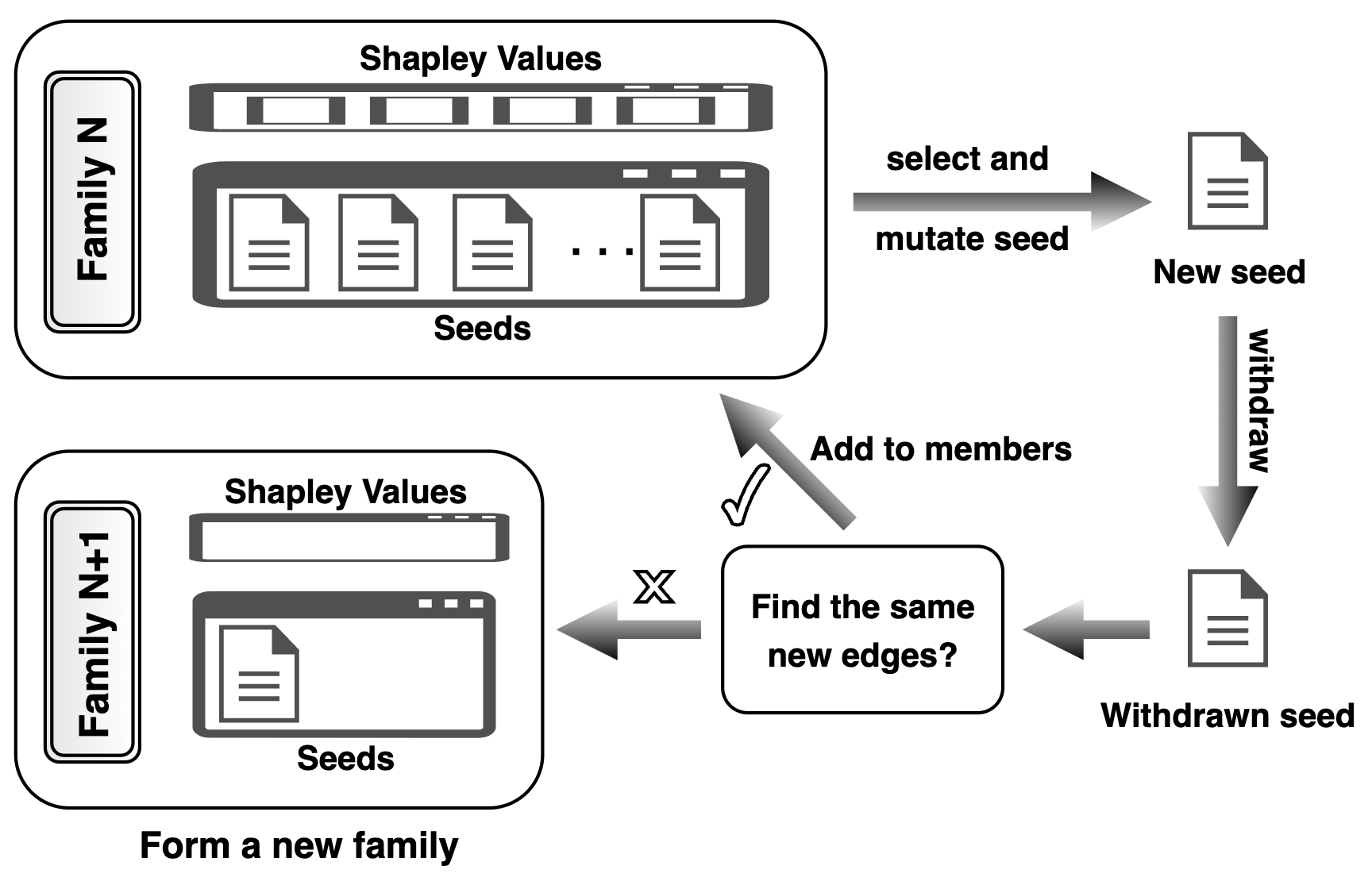
Figure 5: The update of family and family members.

III-B2 Shapley Update During Fuzzing

As mentioned in Section III-A3, Shapley values are calculated for the original seed in a family, which can significantly improve the efficiency of fuzzing. To further improve the efficiency of fuzzing, we update Shapley values by 1) ignoring the generated inputs that do not discover self-new edges, and 2) reducing the combinations of bytes when self-new edges are discovered. If a mutation does not discover self-new edges, then $\mathcal{F}(\ast)=0$. Therefore, the Shapley value remains the same and we do not need to update it. If a cooperative mutation discovers self-new edges, we remove the redundant bytes that do not influence the result of self-new edges. If fuzzing mutates bytes $M_{b}=\{b_{1},b_{2},...,b_{n}\}$ to discover self-new edges, for a redundant byte $b_{i}$, we get $\mathcal{F}(M_{b}\backslash\{b_{i}\})=\mathcal{F}(M_{b})$. This immediately derives that the value of the related $\varphi$ is zero. Therefore, we do not need to update Shapley values for redundant bytes. For the necessary bytes that influence the result of self-new edges, denoted as $N_{b}$, exclusion of any byte $b_{j}$ in $N_{b}$ will not discover self-new edges, i.e., $\mathcal{F}(N_{b}\backslash\{b_{j}\})=0$. Therefore, all necessary bytes in this mutation have the same value of $\varphi$, indicating that we can only calculate $\varphi$ for one necessary byte to update Shapley values for all necessary bytes. In fuzzing, when self-new edges are discovered, we recover mutations of bytes to check whether those bytes are redundant. If the recovery of the mutation of a byte does not change the result of self-new edges, the byte is a redundant byte. To simplify the computation, we consider the mutated bytes, excluding the redundant bytes, as necessary bytes.

III-B3 Family Update

The family for seeds can reduce the overhead of calculating Shapley values because Shapley values for one seed can be shared with multiple seeds. The key of building a family is that the mutation does not change the length of original seeds. Yet, some mutators, such as deletion of bytes, in fuzzing will change the length of seeds. To enrich family members, ShapFuzz will withdraw all mutators that change length when new code are discovered. If the result can still find the same new edges after withdrawing those mutators, ShapFuzz will retain the result of withdrawing to the family. For example, as shown in Figure 5, we select a seed from family $N$ and mutate it. If an input $i_{1}$ discovers new edges, ShapFuzz will withdraw all mutators that change length, which generates another input $i_{2}$. If $i_{2}$ can still find the same new edges that $i_{1}$ finds, ShapFuzz retains $i_{2}$ as a new seed and adds it to the family $N$. Otherwise, $i_{1}$ will form a new family $N+1$ if mutation of $i_{1}$ can further discover new edges. As a result, ShapFuzz has a reasonable number of families and a number of family members.

III-C Shapley-guided Byte Selection

The insight from Section II indicates that more energy can be assigned to bytes with higher Shapley values. In this section, we present Shapley-guided byte selection while the mutation of byte values is performed by AFL++. However, since the Shapley value is calculated based on part of all possible inputs during fuzzing, it cannot guarantee that the bytes with high Shapley values can always maintain high. Besides, seeds share the byte importance with the original seed in the same family. Although a byte may have a high Shapley value, the difficulty of solving path constraints varies in different execution paths. When some bytes are frequently selected but with no new edges discovered, we do not want to waste more energy on those bytes. Therefore, we need to balance the trade-off between mutating high Shapley value bytes and low-frequently chosen bytes.

To maximize code discovery, ShapFuzz uses Contextual Multi-armed Bandit (CMAB) [23, 19] to achieve the trade-off in using Shapley values. Based on the experience of playing arms, CMAB tries to maximize the rewards of playing multi-armed bandits, taking into account the personality of a player (i.e., the context). The trade-off in CMAB is between 1) focusing on the arms with higher historical performance and 2) updating rewards for all arms. This exactly fits into our problem of selecting bytes based on Shapley values.

With Shapley values, ShapFuzz uses CMAB to build a probability distribution for selecting bytes. To build the probability distribution, CMAB calculates scores for each byte. The bytes with higher scores are assigned with higher probabilities. Given a seed $s$, the feature vector $f_{s}$ extracted from the corresponding execution path (i.e., the context), and a byte $p$, the score of the byte is calculated as:

$$Score(s,p)=E[\phi_{p}|f_{s}]+0.5U_{s,p},$$ (5)

where $E[\phi_{p}|f_{s}]$ is the expected reward, $U_{s,p}$ is the upper confidence bound, and $\phi_{p}$ is the Shapley value of byte $p$. As mentioned, the same $\phi_{p}$ in different execution paths has different influence on discovering new code. Therefore, we use $f_{s}$ to represent the context of $\phi_{p}$, and $f_{s}$ is extracted based on its edges in the execution path. First, we find ten center seeds in the seed corpus whose paths are as far as possible from each other. Then, for a seed $s$, we compute the cosine similarity between the path exercised by that seed and the paths exercised by ten center seeds to obtain a fixed dimensional vector $f_{s}$.

To calculate $E[\phi_{p}|f_{s}]$ and $U_{s,p}$, the byte $p$ needs to maintain a tuple $(D_{p},R_{p})$, where $D_{p}$ is a matrix about all history feature vectors and $R_{p}$ is a vector about Shapley values. To update the tuple $(D_{p},R_{p})$:

$$\begin{split}D_{p}&\leftarrow D_{p}+f_{s}f^{T}_{s}\\ R_{p}&\leftarrow R_{p}+\phi_{p}f_{s}\end{split}$$ (6)

Expected Reward. In our model, the expected reward can be calculated by:

$$E[\phi_{p}|f_{s}]=f_{s}^{T}\hat{\theta},$$ (7)

where $\hat{\theta}$ is the best coefficient vector, and it can be estimated by applying ridge regression to the tuple $(D_{p},R_{p})$:

$$\hat{\theta}=(D_{p}^{T}D_{p}+I_{k})^{-1}D_{p}^{T}R_{p},$$ (8)

where $I_{k}$ is a $k$-dimensional identity matrix, and $k$ is the dimension of the feature vector $f_{s}$.

Upper Confidence Bound. The second part of the score is the upper confidence bound $U_{s,p}$, which can be calculated by [34]:

$$U_{s,p}=\sqrt{f_{s}^{T}(D_{p}^{T}D_{p}+I_{d})^{-1}f_{s}}$$ (9)

The more times a byte is selected, the smaller its $U_{s,p}$ is. Thus, the $U_{s,p}$ intends to assign more energy to the bytes that have been less frequently selected, i.e., the bytes with low Shapley values. When bytes with high Shapley values are selected frequently, their scores will be decreased, as well the selection probability. As a result, the score calculated by Equation (5) achieves the trade-off for Shapley-guided fuzzing.

The scores calculated for bytes are further utilized to generate probabilities for selecting bytes. A byte with a higher score is assigned a higher probability. For each mutation, ShapFuzz first randomly sets a number $n$, which is the number of times to perform sub-mutations. That is, it will perform the sub-mutation by $n$ times in one mutation. Then, each time the fuzzer decides which byte to be sub-mutated, the fuzzer will use the probability distribution to select.

III-D Threats to Validity

While our approach has shown promising performance and effectiveness, there are still certain potential factors that could constrain the practical application of ShapFuzz.

III-D1 Overhead of Shapley Calculation

ShapFuzz models the process of byte mutation as a cooperative game and uses Shapley analysis to quantify the contribution of each byte. Assume that self-new edges are found in a mutation, and the number of its mutated positions is $N$. To calculate the Shapley value, we need to analyze the number of self-new edges found in $2^{N}$ subsets of mutated positions. To reduce the overhead, ShapFuzz uses two special cases to simplify the process of Shapley analysis. Firstly, if there are redundant bytes that do not influence the result of the self-new edge, we remove these bytes to reduce $N$. Secondly, if the mutated bytes are necessary for the discovery of self-new edges, these bytes have the same Shapley value. However, if these two conditions are not met and $N$ is large, some overhead will be introduced. In the future, we can use lightweight and improved algorithms of Shapley analysis to alleviate this problem.

III-D2 Changeable Seed Length

Moreover, ShapFuzz builds a family system to alleviate the overhead brought by Shapley analysis. Within a family, all seeds in the same family share the same Shapley values for bytes. However, when maintaining a family, we ignore mutated inputs that change length. This is because the use of mutators that change seed length may disorder byte positions in seeds, and we cannot achieve position mapping between seeds. We can study the mathematical theory for the Shapley analysis of the changeable length in the future. In the existing version, if a new seed is generated by changing length, we use this seed to create a new family to alleviate this problem.

III-D3 The Impact of Self-New Edges

As new edge discovery becomes progressively more difficult over time, ShapFuzz utilizes self-new edges as a metric to measure gains and identify bytes that may impact multiple branches. Nevertheless, in some cases, bytes that contribute to the self-new edges may not necessarily lead to the discovery of extra new edges. The self-new edges might have already been discovered by other seeds. Therefore, bytes with high Shapley values could actually contribute less than what the Shapley values indicate. If we allocate too much energy to these bytes, it could lead to a decrease in fuzzing efficiency. For example, suppose byte $i$ in a seed is related to $y$ edges. If all these $y$ edges have been explored, we can deduce that byte $i$ has made a significant contribution. However, since all the edges related to byte $i$ have been explored, allocating any amount of energy to byte $i$ will not help discover new edges.

III-D4 Semantic Consistency Within Families

To reduce the overhead of calculating Shapley values, the seeds in a family share the same Shapley values. However, despite implementing a strict family construction method (seeds with genetic relationships and the same lengths), there may still be cases where the semantics between seeds are inconsistent. Semantic inconsistency can lead to bytes with different meanings sharing the same Shapley value, thereby incorrectly estimating the importance of bytes. For instance, a length field can often determine the semantics of the following bytes. In such a case, our method cannot guarantee semantic consistency between seeds. Suppose there is a seed $A$, where a byte $i$ is a length field. Seed $B$ is derived from the seed $A$ by mutating the byte $i$. As the change in the length field directly alters the meaning of the subsequent bytes, it is likely that a byte $j$, which follows the byte $i$, in the seed $A$ and seed $B$ (with the same position) carries different meanings. This means that even if seeds $A$ and $B$ have the same length and genetic relationship, the byte $j$ in seed $A$ and seed $B$ is not semantically consistent. If we continue to share the Shapley value of the byte $j$ among these two seeds, it would result in inaccurate Shapley values, enabling some inefficient bytes to be allocated with higher mutation energy, thereby affecting fuzzing efficiency.

IV Evaluation

We implement our ShapFuzz based on AFL++ [10], which integrates many state-of-the-art fuzzing algorithms. We mainly modify the mutation process and the byte schedule. In the evaluation, we evaluate our ShapFuzz with byte-scheduling fuzzers and commonly used fuzzers. To ensure fair results, we conduct our experiments on two third-party testing platforms, UNIFUZZ [21] and MAGMA [14]. Our experiments are performed on a system running Ubuntu 18.04 with 103 cores (Intel(R) Xeon(R) Gold 6230R CPU) and 256 GB of memory. Each fuzzer uses one CPU core to run one target program.

TABLE I: Target programs from UNIFUZZ.

Targets	Projects	Input formats	Test instructions
tiff2bw2	libtiff 3.9.7	tiff	tiff2bw @@1  /dev/null
tiffsplit			tiffsplit @@ /dev/null
tiff2pdf2			tiff2pdf @@ /dev/null
nm	binutils-2.28	ELF	(-A -a -l -S -s
			–special-syms –synthetic
			–with-symbol-versions -D @@)
objdump			-S @@
readelf2			-a @@
size2			@@
pdftotext	pdftotext 4.00	pdf	@@ /dev/null
infotocap	jasper 2.0.12	text	-o /dev/null @@
mp42aac	Bento4 1.5.1-628	mp4	@@ /dev/null
tcpdump	tcpdump 4.8.1 +	tcpdump100	-e -vv -nr @@
	libpcap 1.8.1
flvmeta	flvmeta 1.2.1	flv	@@
lame3.99.5	lame 3.99.5	wav	@@ /dev/null
imginfo	ncurses 6.1	jpg	-f @@
mujs	mujs 1.0.2	js	@@
exiv2	exiv2 0.26	jpg	@@

• @@: A placeholder indicating that the input is a file.

• tiff2bw, tiff2pdf, readelf and size are not from UNIFUZZ

Evaluation Metrics. We use afl-showmap in AFL++ to count the number of edges and compile target programs with ASAN [29] enabled. When analyzing unique bugs, we use the top-three rule to de-duplicate bugs [16].

Target Programs and Initial Seeds. We select 16 commonly used programs for testing from UNIFUZZ and other papers, as shown in the Table I. For each target program, all fuzzers use the same initial seeds, which are collected from UNIFUZZ, FuzzBench[27] and public seed corpus. Most target programs have multiple initial seeds as suggested by Adrian Herrera [15].

TABLE II: Edge Coverage and Analysis Time comparison between different fuzzers (on ALL SEEDS).

Programs		ShapFuzz			GreyOne			ProFuzzer			Angora			PreFuzz			NEUZZ
Name	Len	Cov.	Time	#Bug	Cov.	Time	#Bug	Cov.	Time	#Bug	Cov.	Time	#Bug	Cov.	Time	#Bug	Cov.	Time	#Bug
tiff2pdf	448	4401	85s	0	4486	35207s	0	4578	12694s	1	2314	235s	0	3475	G	1	2832	G1	1
lame	13818	3656	3985s	5	3645	80225s	4	3649	70003s	4	2265	5813s	4	-	-	0	-2	-	0
readelf	272030	5611	1048s	4	5058	78788s	3	5168	74878s	6	5786	3758s	6	-	-	0	-	-	0
exiv2	25633	3790	135s	15	3626	35401s	5	3698	32311s	12	4291	615s	11	2866	G	0	-	-	0
flvmeta	16454	230	0s	2	230	32782s	2	230	11625s	2	230	201s	2	-	-	0	-	-	0
nm	272030	3136	248s	17	2628	83058s	9	2750	81747s	10	2657	2351s	51	-	-	0	-	-	0
tiffsplit	10032	1709	5s	7	1699	13398s	5	1719	6220s	6	890	291s	1	1189	G	2	1113	G	1
tiff2bw	10032	1839	87s	6	1870	12709s	6	1848	8702s	5	1180	310s	1	1651	G	0	1441	G	0
objdump	272030	4958	742s	14	3864	79211s	4	4106	83913s	5	3192	3672s	3	-	-	0	-	-	0
pdftotext	12465	6613	3508s	23	5794	80548s	2	5777	80591s	3	4250	14801s	2	4902	G	5	4394	G	0
mp42aac	31988	1266	19s	2	1144	75949s	0	1166	66141s	0	1120	540s	0	1017	G	0	950	G	0
tcpdump	6983	12764	328s	1	11558	50599s	1	11879	29383s	0	7615	2510s	3	4672	G	0	6019	G	0
mujs	6983	4136	0s	0	4020	18157s	0	3979	7181s	0	2364	8829s	0	2432	G	0	2393	G	0
size	272030	1860	188s	0	1667	77562s	0	1690	78671s	0	1988	2032s	0	-	-	0	-	-	0
infotocap	2519	1817	276s	7	1670	39193s	6	1530	44335s	5	940	1104s	0	1266	G	1	1071	G	0
imginfo	2519	1895	30s	0	1818	36298s	0	1744	43274s	0	1384	184s	0	-	-	0	-	-	0
Total		59681		103	54777		47	55511		59	42466		84	23470		9	20213		2

• G: A GPU is required to train the model.

• -: The fuzzer fails to run on this program due to large input size.

TABLE III: Edge Coverage and Analysis Time comparison between different fuzzers (on SEEDS<10000).

Programs		ShapFuzz			GreyOne			ProFuzzer			Angora			PreFuzz			NEUZZ
Name	Len	Cov.	Time	#Bug	Cov.	Time	#Bug	Cov.	Time	#Bug	Cov.	Time	#Bug	Cov.	Time	#Bug	Cov.	Time	#Bug
tiff2pdf	448	4461	30s	1	4450	39189s	0	4552	15278s	0	2306	50s	0	3466	G	0	2543	G1	0
readelf	4230	5359	77s	5	5346	39952s	6	5272	38537s	3	5554	1628s	7	4540	G	6	4208	G	4
exiv2	8437	3882	196s	7	3385	50513s	4	3691	31915s	3	3903	2365s	9	3881	G	0	3151	G	0
nm	4230	2822	17s	30	2818	29069s	20	2884	13905s	22	2409	2056s	35	2260	G	14	1749	G	0
tiffsplit	7222	1718	4s	6	1725	13541s	6	1715	4519s	7	919	219s	3	1203	G	2	1128	G	0
tiff2bw	7222	1882	42s	7	1876	12031s	6	1808	6040s	6	1186	200s	1	1594	G	0	1489	G	0
objdump	4230	4654	104s	16	4145	75874s	10	4414	50760s	13	3085	4182s	13	3560	G	4	3136	G	0
tcpdump	2305	12963	227s	1	12164	40025s	1	12497	13022s	0	7826	2119s	1	7963	G	1	6251	G	0
mujs	2305	4145	0s	0	4000	19877s	0	4015	7078s	0	2383	8677s	0	2589	G	1	2388	G	0
size	4230	1795	22s	0	1785	12623s	0	1812	9547s	0	1794	1259s	1	1458	G	0	1224	G	0
infotocap	2519	1807	457s	8	1767	38278s	5	1399	45154s	2	840	1647s	0	1159	G	1	1074	G	0
imginfo	2519	2486	9s	0	1744	26514s	0	1680	24268s	0	1413	244s	0	1464	G	0	1176	G	0
Total		47974		81	45205		58	45739		56	33618		70	35137		29	29517		4

• G: A GPU is required to train the model.

TABLE IV: Edge Coverage and Analysis Time comparison between different fuzzers (on SEEDS<1000).

Programs		ShapFuzz			GreyOne			ProFuzzer			Angora			PreFuzz			NEUZZ
Name	Len	Cov.	Time	#Bug	Cov.	Time	#Bug	Cov.	Time	#Bug	Cov.	Time	#Bug	Cov.	Time	#Bug	Cov.	Time	#Bug
tiff2pdf	448	4383	99s	1	4493	39407s	0	4449	12856s	1	2459	58s	0	3398	G	1	2709	G1	1
readelf	324	4983	34s	4	4875	13088s	3	4763	5978s	0	5131	299s	5	4144	G	0	3760	G	0
nm	324	1876	2s	0	1872	9869s	0	1891	4521s	0	1838	65s	0	1424	G	0	1103	G	0
tiffsplit	858	1721	4s	6	1712	17187s	4	1697	8743s	6	935	19s	4	1155	G	2	1134	G	0
tiff2bw	858	1882	6s	8	1829	13096s	4	1861	7278s	8	1263	13s	1	1533	G	0	1435	G	0
objdump	324	3629	25s	0	3667	19014s	0	3731	9879s	0	2422	1143s	0	2624	G	1	2275	G	0
tcpdump	451	11594	59s	0	10465	19800s	0	10827	7126s	0	7355	2077s	1	5948	G	0	4499	G	0
mujs	451	4153	0s	0	3973	15638s	0	4027	6055s	0	2421	8605s	0	2590	G	1	2418	G	0
size	324	1752	4s	0	1733	7343s	0	1747	3455s	0	1672	128s	0	1331	G	0	1225	G	0
infotocap	432	1824	131s	7	1782	33321s	6	1679	34827s	5	895	160s	0	1164	G	0	1308	G	0
imginfo	432	1625	2s	0	1494	26077s	0	1611	24070s	0	1307	43s	0	1413	G	0	1105	G	0
Total		39422		26	37895		17	38283		20	27698		11	26724		5	22971		1

• G: A GPU is required to train the model.

IV-A ShapFuzz vs. Byte-Scheduling Fuzzers

In this section, we compare ShapFuzz with five state-of-the-art byte-scheduling fuzzers. We analyze their performance on three sets of initial seeds with different lengths, observing their effectiveness in edge coverage, bug detection, and analysis time.

IV-A1 Compared Fuzzers

There are three main types of existing methods for identifying constraint-related bytes in seed files, including inference-based fuzzers, neural network-based fuzzers, and taint-based fuzzers. In order to compare the performance of ShapFuzz with these three category fuzzer in different scenarios, we designed a diverse set of experiments to analyze the pros and cons of each fuzzer. Specifically, we compared ShapFuzz with five state-of-the-art fuzzers Greyone [12], ProFuzzer [37], NEUZZ [32], PreFuzz [36] and Angora[6].

Inference-based fuzzer. Inference-based fuzzers mutate all bytes of a seed before scheduling mutation, and determine the importance of each byte based on its execution, such as Greyone [12] and ProFuzzer [37]. Greyone iterates over each byte in the input, observing whether the state of a CMP instruction in the program changes. If it does, then the byte is related to the target CMP. ProFuzzer iterates over all 256 values at each byte and determines the type of each byte (e.g., size and offset) based on changes in the path length. However, since these two fuzzers are not open-sourced, we implement their core ideas based on AFL++. For GreyOne, we mutate each byte of the seed and observe whether the number of CMPs with unexplored branches changes. If it does, we consider the byte to be CMP-related. For ProFuzzer, we mutate each byte of the seed four times and observe whether the execution path changes. If it does, we consider the byte to be control flow-related. Finally, we randomly mutate the identified CMP-related bytes or control flow-related bytes.

Neural network-based fuzzer. Neural network-based fuzzers refer to the ones that use neural networks to roughly identify the constraint-related bytes of a seed, such as NEUZZ [32] and PreFuzz [36]. NEUZZ identifies bytes related to program branches using deep learning models. PreFuzz optimizes the edge and byte selection mechanism of NEUZZ.

Taint-based fuzzer. Taint-based fuzzers refer to fuzzers that use taint analysis to analyze the bytes related to path constraints, such as Angora [6]. Angora uses byte-level taint analysis to track which input bytes are related to path constraints.

IV-A2 Experiment Setup

The recognition of constraint-related bytes by inference-based fuzzers, neural network-based fuzzers, and taint-based fuzzers is significantly influenced by the length of the seed. The longer the seed, the longer the analysis time required by these methods. Seeds with long length may fail the execution of existing fuzzers. However, ShapFuzz does not need to analyze each byte of the seed one by one, nor does it require building a neural network model. Therefore, the analysis time of ShapFuzz is not significantly affected by the length of the seed. To analyze the performance of each fuzzer on initial seeds of different lengths, we divide the initial seeds into three groups based on their length and conduct experiments on each of them separately. The length related groups are ALL SEEDS, SEEDS<10000 (seeds that have less than 10,000 bytes), and SEEDS<1000 (seeds that have less than 1,000 bytes). We analyze the analysis time, edge coverage, and bug discovery of each fuzzer in the three experimental environments. All experiments run for 24 hours and repeat 5 times.

IV-A3 Edge Coverage and Analysis Time

Tables II, III and IV show the edge coverage and analysis time achieved by six fuzzers on three sets of different initial seeds. From Table II, with all the initial seeds provided, ShapFuzz discovers a total of 59681 edges, which are 4170 more edges than the second best fuzzer, ProFuzzer. Notably, NEUZZ and PreFuzz only discover 20213 and 23470 edges (about 1/3 edges discovered by ShapFuzz) respectively on 16 programs. On programs like lame, NEUZZ and PreFuzz fail to run the fuzzer because of long seed lengths, resulting in a large model that causes an OOM error during training. As for analysis time, ShapFuzz consistently requires less time to analyze all programs compared to other fuzzers. For example, ShapFuzz uses less than 1000 seconds to analyze 13 programs, while GreyOne and ProFuzzer require more than 10000 seconds for most programs. This is because GreyOne and ProFuzzer have to analyze each byte of the seed before mutation, which means that the analysis time is proportional to the seed length. Angora requires less than 1000 seconds to analyze 7 programs, indicating that the ShapFuzz’s analysis time is still superior to the traditional taint analysis. The average analysis times for ShapFuzz, GreyOne, ProFuzzer, and Angora are 640.37 seconds, 54196.06 seconds, 36174.81 seconds, and 2567.31 seconds, respectively. The average analysis time required by ShapFuzz is only about 2% of Greyone’s. NEUZZ and PreFuzz require an additional GPU for analysis, which consumes a significant amount of resources.

From Table III and IV, as the length of the seed decreases, the analysis time of all fuzzers decreases, particularly for GreyOne and ProFuzzer. For example, with ALL SEEDS, ProFuzzer takes 81747 seconds to analyze nm, but with SEED < 1000, the analysis time decreases to 4521 seconds. Notably, ShapFuzz exhibits the most stable performance among the three experiments and consistently achieves the highest edge coverage on most programs. Finally, ShapFuzz discovers the most total edges across all three experiments.

IV-A4 Unique Bugs

Tables II, III and IV show the number of unique bugs discovered by each fuzzer on three sets of initial seeds. In all cases, ShapFuzz is able to discover more unique bugs than other fuzzers. On ALL SEEDS, ShapFuzz finds 103 unique bugs, which is 19 more than the best performing comparison fuzzer, Angora. On SEEDS<10000, ShapFuzz discovers 81 unique bugs, which is 11 more than the second-ranked fuzzer, Angora. On SEEDS<1000, ShapFuzz discovers 40 unique bugs, which is 3 more than the best performing comparison fuzzer, ProFuzzer. Notably, we find that a fuzzer’s performance in terms of edge coverage and bug discovery is not always consistent. For example, although Angora does not perform as well as GreyOne and ProFuzzer in terms of edge coverage, it still discovers more bugs. ShapFuzz achieves the best performance in both edge coverage and bug discovery.

Further analysis shows that ShapFuzz finds 36 bugs that are not found by any other fuzzers. Among the 36 bugs, 18 of them come from the code that is explored but without crashing it by the others while the remaining 18 of them come from completely new code regions.

IV-A5 Bug Intersection Analysis

We compute set differences and intersections for bugs in Table II. The results are shown in Table V. ShapFuzz discovers 64, 52, 75, 102, and 96 bugs that are not found by GreyOne, ProFuzzer, Angora, NEUZZ, and PreFuzz, respectively. GreyOne, ProFuzzer, NEUZZ, and PreFuzz detect fewer than 10 bugs that are not found by ShapFuzz, but Angora detects 54 bugs that ShapFuzz misses. Further analysis reveals that Angora performs well on the program nm by finding 39 bugs that ShapFuzz misses. However, ShapFuzz discovers 479 more new edges than Angora. We believe that Angora’s lower efficiency in discovering new edges is due to its constraint analysis method, which explores constraints one by one. Angora’s constraint prioritization strategy might contribute to its ability to finding more bugs, but this could be coincidental. ShapFuzz’s limited exploitation capability may also be a reason for its mediocre performance on some programs.

TABLE V: Set differences and intersections for bugs in Table II.

	GreyOne	ProFuzzer	Angora	NEUZZ	PreFuzz
ShapFuzz & *1	39	51	30	1	7
ShapFuzz - *2	64	52	73	102	96
- ShapFuzz3	8	8	54	1	2

• ShapFuzz & *: the intersection of bugs found by both ShapFuzz and the other fuzzers.

• ShapFuzz - *: the number of bugs found by ShapFuzz but not by the other fuzzers.

• * - ShapFuzz: the number of bugs found by other fuzzers but not by ShapFuzz.

IV-B ShapFuzz vs. Commonly Used Fuzzers

In this section, we compare ShapFuzz with some commonly used fuzzers to further demonstrate its superior performance. To ensure fair results, we conduct our experiments on two third-party testing platforms, UNIFUZZ [21] and MAGMA [14]. All experiments run for 24 hours and repeat 10 times to avoid the randomness of fuzzing [4].

IV-B1 Compared Fuzzers

We compare ShapFuzz with the state-of-the-art CGFs, including AFL [40], AFL++ [10], AFLFast [3], FairFuzz [18], MOPT [25], and EMS [26]. In this section, we use the AFL, AFLFast, MOPT, and FairFuzz implemented within AFL++ for our experiments. AFL is a popular fuzzer that is the basis of many other recent fuzzers [3, 18, 25, 38, 26, 32]. AFL++ is a framework that integrates many state-of-the-art fuzzers into AFL, such as MOPT, AFLfast and Redqueen. In our evaluation, We enable AFL++’s Redqueen mutator and MOPT mutator, which is the best-performing configuration of AFL++. AFLFast models the fuzzing process as a Markov chain and prioritizes low-frequency paths to achieve better code coverage. FairFuzz proposes a novel mutation mask to guide fuzzing towards rare branches. MOPT utilizes Particle Swarm Optimization to optimize the schedule of mutation operators based on fuzzing history. For MOPT and MOPT related fuzzers, we set $-L=5$.

IV-B2 Edge Coverage

To evaluate the efficiency of edge discovery, we evaluate fuzzers by using the ranks of edge discovery after fuzzing 1/3/24 hours. The lower the rank is, the better the fuzzer performs. As shown in Figure 6, the performance of most fuzzers at different running hours is not significantly different. Yet, Figure 6 indicates that ShapFuzz achieves better code coverage on most programs than other fuzzers. After fuzzing for 1 and 3 hours, the median rank of ShapFuzz is 1.5 and 1.5, respectively, which indicates that the fuzzing efficiency of ShapFuzz in a short period of time is higher. After fuzzing 24 hours, the median rank of ShapFuzz is 1.81. This indicates that ShapFuzz’s strategy is more efficient than MOPT whose the median rank is 4.75.

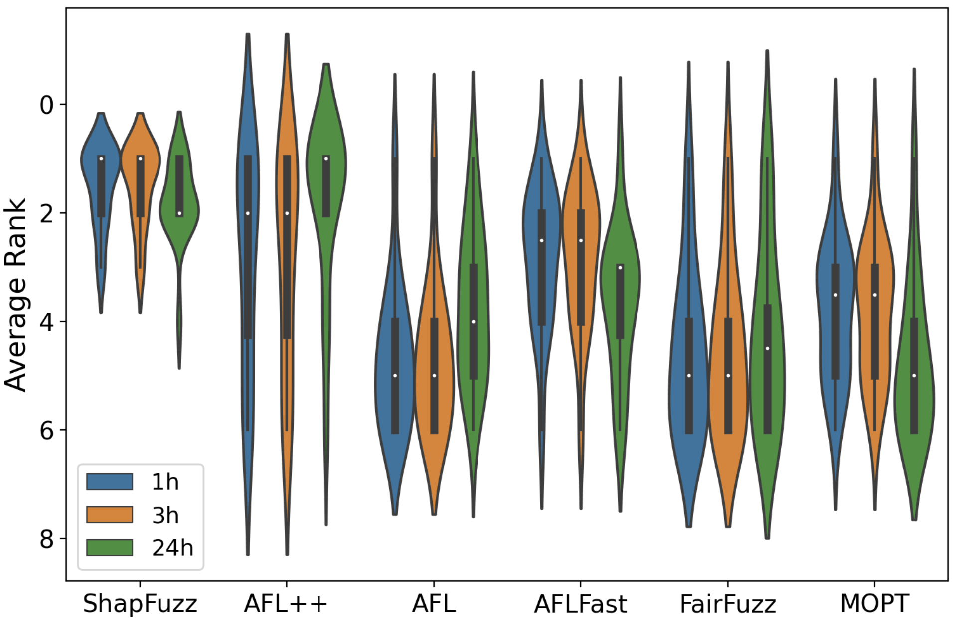
Figure 6: The violin plot of average edge ranks across 10 trials of different fuzzers after running for 1/3/24 hours.

TABLE VI: The number of unique bugs discovered by different fuzzers (on UNIFUZZ).

Programs	ShapFuzz	AFL++	MOPT	AFL	AFLFast	FairFuzz
tiff2pdf	1	2	1	0	0	0
lame	4	4	4	5	4	4
readelf	6	4	4	3	5	5
exiv2	18	23	3	15	15	14
flvmeta	2	2	2	2	2	2
nm	35	31	21	22	22	30
tiffsplit	7	9	7	5	7	5
tiff2bw	10	6	5	5	5	7
objdump	29	11	8	12	10	8
pdftotext	27	24	20	25	24	23
mp42aac	0	5	0	0	0	0
tcpdump	2	1	0	2	1	2
infotocap	11	9	9	5	9	9
imginfo	0	1	0	2	0	0
Total	152	132	84	103	104	109

IV-B3 Bug Discovery on UNIFUZZ

We analyze the number of unique bugs triggered by a fuzzer based on ASAN. Following the guidance of UNIFUZZ [21], we select the top three stack frames to de-duplicate bugs. Table VI shows the number of unique bugs triggered by each fuzzer. ShapFuzz, MOPT, AFLFast, FairFuzz, AFL, and AFL++ trigger 152, 84, 103, 104, 109 and 132 bugs, respectively. ShapFuzz finds the most bugs in 16 programs, with 20 more bugs than AFL++. Specifically, ShapFuzz performs the best on 8 programs, including nm, readelf, flvmeta, tiff2bw, objdump, pdftotext, tcpdump and infotocap. Surprisingly, MOPT and AFLFast do not perform the best on any program. AFL++, AFL and FairFuzz only perform the best on 5, 3 and 1 programs, respectively. In summary, ShapFuzz performs the best on most of the programs, demonstrating the effectiveness of ShapFuzz.

Furthermore, we use ShapFuzz to test some of the latest versions of programs and successfully found several previously unknown bugs. The results are shown in the Table VII. We find 11 bugs in 6 programs. Particularly, two bugs have been confirmed by developers as previously undiscovered bugs, and one bug has been fixed in the beta version. The four bugs in jhead have been fixed in the new version before receiving a response. The remaining 4 bugs are still being confirmed.

TABLE VII: New bugs discovered by ShapFuzz on the latest versions of programs.

Programs	Known Vulnerabilities	Unknown Vulnerabilities	Sum
infotocap	0	1	1
imginfo	0	1	1
mp42aac	(submitted)1	(submitted)	2
jhead	4	0	4
cflow	(submitted)	(submitted)	2
mujs	1	0	1
Total			11

• (submitted): We have submitted the bugs and have no response yet.

IV-B4 Overhead

ShapFuzz adds some extra steps to AFL++, including tracing mutators, recovering mutators, and calculating the Shapley Values of bytes. Thus, to quantify the influence of these steps on fuzzing throughput (i.e., execution speed), we measure the total number of executions for each fuzzer. Figure 7 shows the total number of executions of all 16 programs that fuzzers run after 24 hours. The results show that the throughput of ShapFuzz does not drop significantly comparing to other fuzzers. After fuzzing 24 hours, the throughput of ShapFuzz is lower than that of MOPT, AFL++, AFL and AFLFast by 6.16%, 7.91%, 10.25%, 8.38%, respectively. However, the total throughput of ShapFuzz is higher than FairFuzz by 9.75%. Surprisingly, on programs tiffsplit and exiv2, the throughput of ShapFuzz is higher than AFL++, MOPT, AFL and FairFuzz. Therefore, our ShapFuzz does not introduce much overhead.

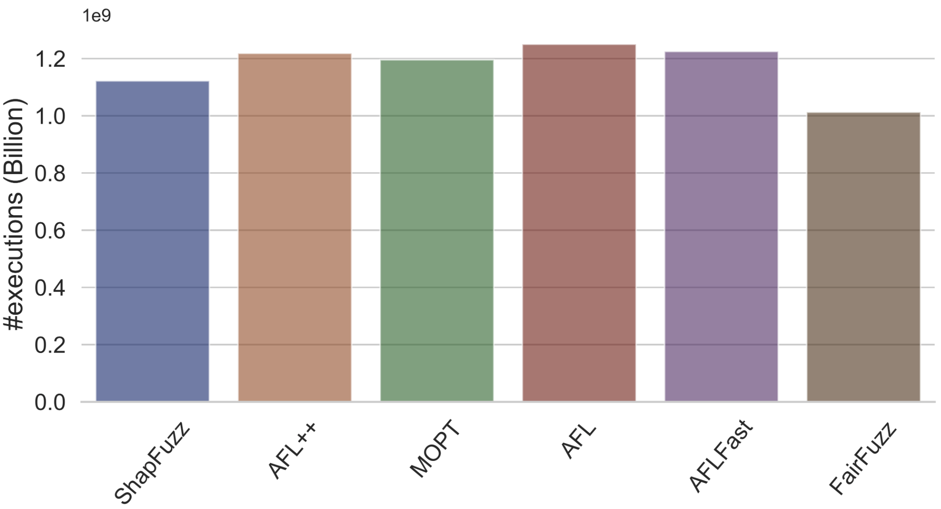
Figure 7: The total throughput of different fuzzers running for 24 hours.

IV-B5 Evaluation on MAGMA

TABLE VIII: Target programs from MAGMA.

Projects	Target Programs	Input format
libpng 1.6.38	libpng_read_fuzzer	PNG
libtiff 4.1.0	read_rgba_fuzzer, tiffcp	TIFF
libxml2 2.9.10	libxml2_xml_read_memory_fuzzer, xmllint	XML
poppler 0.88.0	pdf_fuzzer, pdfimages	PDF
openssl 3.0.0	asn1, asn1parse, bignum, server, client, x509	Binary blobs
sqlite3 3.32.0	sqlite3_fuzz	SQL queries
php 8.8.0	exif, json, parser, unserialize	Various
libsndfile	sndfile_fuzzer	WAV
lua	lua	LUA

To further evaluate the bug-finding performance of ShapFuzz, we conduct experiments on MAGMA. MAGMA is a ground-truth fuzzing benchmark that enables accurate and consistent fuzzing evaluation. MAGMA provides several benchmarks with real-world bugs, and it can perform a realistic evaluation of fuzzers. We integrate our ShapFuzz into MAGMA, and compare them to 5 widely-used mutation-based fuzzers (i.e., AFL, AFLFast, FairFuzz, MOPT and AFL++). AFL++ is the AFL++ that enables both MOPT and Redqueen. Due to configure issues of MAGMA, we use the original implementations of fuzzers rather than the implementations based on AFL++. Table VIII shows the target programs used in MAGMA.

Bug Discovery. Table IX shows the number of CVEs triggered by each fuzzer on average. It shows that ShapFuzz performs the best on MAGMA and it exposes the most bugs on 7 of 9 programs. Specifically, ShapFuzz performs the best on libsndfile, libxml2, lua, openssl, php, poppler and sqlite3, exposing 7.00, 4.22, 1.00, 4.00, 3.00, 5.56 and 4.56 bugs on average, respectively. Moreover, ShapFuzz performs significantly better than all the other fuzzers on openssl, poppler and sqlite3. On splite3, ShapFuzz discovers almost two times the number of bugs compared to AFL++. Surprisingly, AFL++ only exposes the most bugs on 2 programs.

TABLE IX: The average number of bugs found by different fuzzers (on MAGMA).

Programs	ShapFuzz	AFL++	AFL	AFLFast	FairFuzz	MOPT
libpng	1.44	2.22	1.89	1.00	1.56	1.56
libsndfile	7.00	6.89	2.89	2.33	1.44	4.78
libtiff	5.89	6.22	5.44	4.22	4.67	5.67
libxml2	4.22	4.00	1.00	1.89	1.00	2.78
lua	1.00	0.56	1.00	1.00	0.89	1.00
openssl	4.00	2.67	3.11	3.33	2.44	3.00
php	3.00	2.00	3.00	3.00	2.56	3.00
poppler	5.56	4.33	3.00	3.44	2.22	3.44
sqlite3	4.56	2.56	0.89	1.78	0.89	0.67
#The Best1	7	2	2	2	0	2

• #The Best: the number of programs that a fuzzer performs the best.

Time to Bug. We analyze the first time that each bug is found and the results are shown in the Table X. In 10 trials, a total of 48 bugs are found by these 7 fuzzers. Among them, ShapFuzz performs the best, with a total of 46 discovered bugs. Additionally, among the bugs discovered by ShapFuzz, 7 bugs cannot be exposed by AFL++, MOPT, FairFuzz, AFL and AFLFast. As for TTB, ShapFuzz has the least time to bug (TTB) on 29 CVEs, which is the best performance among fuzzers. For example, for 25 bugs, ShapFuzz discovers them 2$\times$ faster than AFL++. Note that, CVE-2017-2518 and CVE-2019-19317, CVE-2017-9776, CVE-2013-7443, CVE-2019-19880, PDF008 and CVE-2019-19646 can only be exposed by ShapFuzz. Due to the advantage of solving path constraints, ShapFuzz exposes bugs in less time than others.

TABLE X: The time to bug (TTB) of fuzzers (on MAGMA). ShapFuzz performs the best in discovering bugs.

Vulnerabilities	ShapFuzz	AFL++	MOPT	FairFuzz	AFL	AFLFast
CVE-2015-8472	17s	23s	15s	15s	15s	15s
CVE-2016-1762	47s	1m	15s	20s	16s	18s
CVE-2018-13988	1m	1m	52s	2m	1m	1m
CVE-2016-2109	3m	4m	1m	2m	1m	2m
CVE-2016-6309	4m	5m	1m	2m	1m	1m
CVE-2016-10270	23s	48s	19m	3m	23m	11m
CVE-2016-3658	4m	17m	1h	25m	1h	1h
CVE-2018-14883	18m	1h	3m	2h	2m	3m
CVE-2017-6892	13m	32m	33m	3h	13m	1h
SND017	4m	5m	25m	21h	38m	5m
CVE-2017-11613	9m	1h	1h	15h	6h	4h
CVE-2019-11034	6h	15h	1m	8m	2m	1m
PDF010	3h	1h	7h	16h	10h	2m
CVE-2019-7663	3h	8h	4h	9h	16h	6h
CVE-2019-20218	49m	2h	16h	11h	9h	9h
CVE-2019-9638	41m	17h	7h	17h	4h	44m
CVE-2015-8317	22m	1h	3h	-	-	12h
CVE-2019-7310	7h	17h	9h	15h	7h	8h
CVE-2020-15945	5h	4h	14h	15h	13h	16h
SND020	16m	19m	7h	21h	-	-
CVE-2015-3414	1h	4h	17h	16h	23h	15h
CVE-2016-10269	2h	1h	15h	22h	15h	-
CVE-2011-2696	18m	22m	17h	-	22h	23h
CVE-2017-8363	13m	28m	18h	22h	-	-
CVE-2017-8363	27m	32m	18h	22h	-	-
CVE-2017-9047	33m	6h	12h	-	-	-
CVE-2017-8361	14m	3h	18h	22h	-	-
CVE-2016-6302	9h	23h	16h	-	3h	6h
CVE-2017-7375	6h	1h	-	-	-	-
CVE-2018-10768	5h	5h	23h	-	-	23h
CVE-2016-5314	19h	19h	11h	16h	4h	-
CVE-2013-6954	13h	19h	16h	12h	11h	-
CVE-2019-19926	5h	19h	17h	-	21h	20h
PNG006	-	6m	-	-	-	-
CVE-2016-2108	3h	16h	22h	-	-	-
CVE-2016-10269	23h	2h	22h	-	-	-
CVE-2017-9865	8h	12h	-	-	-	-
CVE-2015-8784	22h	21h	20h	18h	-	20h
CVE-2016-1836	22h	23h	-	-	-	-
CVE-2017-14617	-	21h	-	-	-	-
CVE-2017-3735	20h	-	5h	15h	22h	10h
CVE-2017-9776	19h	-	-	-	-	-
CVE-2013-7443	17h	-	-	-	-	-
CVE-2019-19880	18h	-	-	-	-	-
PDF008	20h	-	-	-	-	-
CVE-2019-19646	22h	-	-	-	-	-
CVE-2017-2518	22h	-	-	-	-	-
CVE-2019-19317	22h	-	-	-	-	-
#The Fastest1	29	7	7	2	9	4

• #The Fastest: The number of vulnerabilities that are discovered the fastest by the fuzzer.

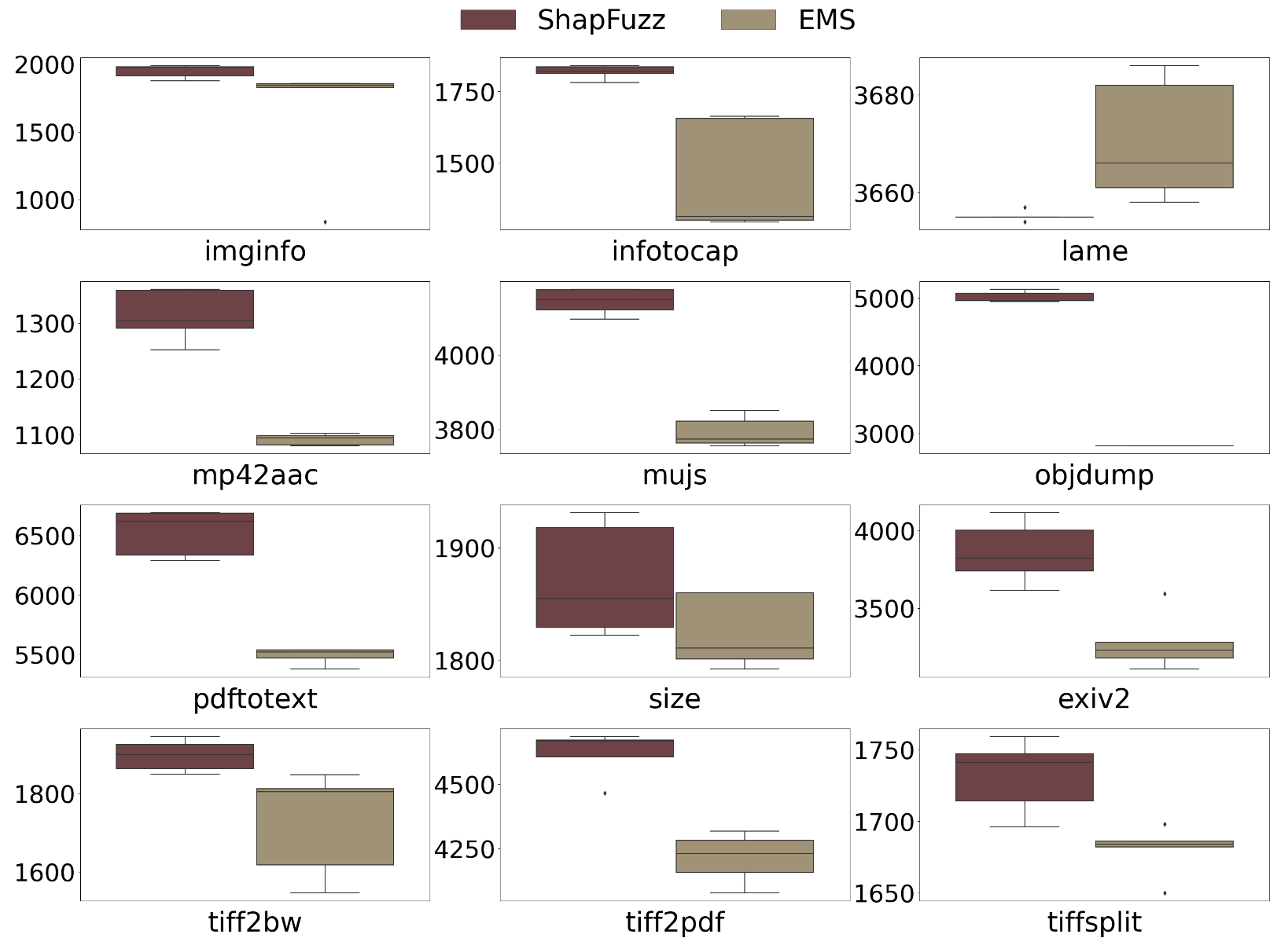
Figure 8: The boxplot of edge coverage for ShapFuzz and EMS. Y-axis: the number of discovered edges.

IV-C Comparison with Byte Mutation Solution

EMS is the latest fuzzer focusing on byte mutation, which reuses history byte values that trigger unique paths and crashes. Specifically, EMS finds that the fuzzing history, both within and across trials, contains valuable mutation strategies that can lead to the discovery of new paths or crashes sharing similar partial path constraints. Because some programs will occupy tens of GB of memory when tested by EMS (implementation issues of EMS), we run experiments with part of the programs on Table I. To ensure data consistency, we use afl-showmap of AFL++ to count the number of edges for EMS and ShapFuzz. The results of edge coverage discovered by ShapFuzz and EMS are shown in the Figure 8. Except for the program lame, ShapFuzz performs better than EMS. Specifically, the median of edge coverage discovered by ShapFuzz is higher than EMS by 6.78%, 27.89%, 16.10%, 9.01%, 43.13%, 16.57%, 2.37%, 15.51%, 5.00%, 9.38% and 3.27% on imginfo, infotocap, mp42aac, mujs, objdump, pdftotext, size, exiv2, tiff2bw, tiff2pdf and tiffsplit, respectively. As to the performance of unique bugs discovered by the two fuzzers, the results are shown in Table XI. ShapFuzz triggers more bugs on 6 programs, while EMS only triggers more bugs on 2 programs. Our ShapFuzz discovers 90 bugs on these programs while EMS only discovers 39 bugs.

TABLE XI: The number of unique bugs discovered by ShapFuzz and EMS (on UNIFUZZ).

Programs	EMS	ShapFuzz
lame	4	4
exiv2	13	15
tiffsplit	8	6
tiff2bw	8	8
objdump	1	15
pdftotext	1	25
mp42aac	1	0
infotocap	3	10
tiff2pdf	0	2
readelf	0	5
Total	39	90

IV-D Ablation Study of ShapFuzz

ShapFuzz has two main components that are calculation of Shapley values (Sections III-A and III-B) and Shapley-guided byte selection (Section III-C). Since Shapley-guided byte selection cannot be performed without Shapley values, we do not compare this component. Since the process of calculating the Shapley value introduces some additional mutations, we want to analyze the impact they have. To analyze the impact of calculating Shapley values, we implement ShapFuzz-modeling to compare with ShapFuzz. For ShapFuzz-modeling, we remove the Shapley-guided byte selection and randomly select positions to mutate.

We evaluated two fuzzers ShapFuzz and ShapFuzz-modeling in UNIFUZZ for 24 hours for 5 times. The result is shown in the Figure 9. With the help of Shapley-guided mutation, ShapFuzz discovers more new edges under most procedures. For instance, the median of ShapFuzz is higher than ShapFuzz-modeling on objdump, nm, tiffsplit, lame, exiv2, tiff2bw, tcpdum and mp42aac. It illustrates that Shapley-guided mutation can indeed generate a more useful mutation possibility distribution for seeds.

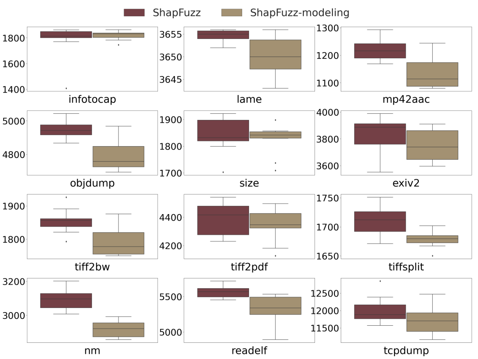
Figure 9: The boxplot of edge coverage for ShapFuzz and ShapFuzz-modeling. Y-axis: the number of discovered edges.

IV-E Comparison with Inference-based Fuzzers

In this section, we compare ShapFuzz with inference-based fuzzers, including GreyOne [12] and ProFuzzer [37], in terms of the effectiveness of inferred bytes.

Experiment Setup. We randomly select 10 target programs and several initial seeds for experiments from UNIFUZZ. To compare the efficiency gap between the Shapley bytes identified by ShapFuzz and the CMP-related bytes identified by GreyOne and ProFuzzer, we analyze each initial seed separately, and the specific experimental steps are as follows. For an initial seed, we use ShapFuzz, Greyone and ProFuzzer to infer the Shapley bytes or CMP-related bytes and mutate these bytes randomly for 3 hours, respectively. Then, we count the additional analysis time required by each fuzzer and the number of new edges they discover. In particular, for the convenience of comparison, we do not update the seed queue but continuously mutate the selected initial seed.

Comparison Metrics. We use the following two new metrics for fine-grained analysis of the above fuzzers:

• The proportion of useful bytes: If a byte is inferred and finds a new edge in the subsequent mutation process, it is called a useful byte. For ShapFuzz, we do not count the first time when an inferred byte is retained. We record the proportion of useful bytes in all inferred bytes.

• The average number of useful mutations: If the mutation of inferred bytes finds a new edge, this mutation is a useful mutation. We use this metric to describe the usefulness of each byte. If a byte has more mutations that discover new edges, it is more useful.

Result. We only include seeds that can complete the analysis within three hours. In three hours, ShapFuzz can complete the analysis of all seeds, but both GreyOne and ProFuzzer have some long seeds that cannot complete the analysis. The results are shown in the Table XII. We analyze the average number of useful mutations for each fuzzer at 1,000,000 mutations. ShapFuzz perform the best, and its average proportion of useful bytes is up to 70.5%. Moreover, ShapFuzz’s average number of useful mutations is up to 3.715. The proportion of useful bytes and average number of useful mutations of GreyOne are only 16.1% and 0.947, while that of ProFuzzer are only 17.8% and 0.0887. According to the above experimental results, ShapFuzz can find more useful bytes within shorter analysis time.

TABLE XII: The comparison of position inference. ShapFuzz can infer more useful positions.

Programs	GreyOne		ProFuzzer		ShapFuzz
	UR1	AUM2	UR	AUM	UR	AUM
nm	3%(135/4834)	0.11	16%(109/665)	0.32	67%(55/82)	1.87
tiff2bw	13%(101/762)	0.74	14%(106/762)	0.75	89%(74/83)	5.87
tiffsplit	68%(104/152)	3.18	69%(104/150)	3.25	92%(72/78)	6.60
objdump	2%(205/13288)	0.45	18%(318/1794)	0.68	60%(179/299)	1.70
readelf	3%(99/3798)	0.41	7%(186/2641)	0.48	83%(95/114)	8.70
flvmeta	46%(29/63)	1.28	22%(42/187)	0.46	40%(14/35)	1.08
pdftotext	3%(267/8384)	0.07	4%(337/8805)	0.08	54%(165/305)	1.11
mp42aac	19%(124/651)	0.32	21%(132/614)	0.35	68%(69/102)	1.70
tcpdump	2%(88/4075)	2.89	3%(87/2708)	2.48	77%(72/93)	6.36
lame3.99.5	1%(169/13077)	0.02	1%(179/13060)	0.02	73%(74/102)	2.16
Average	16%	0.947	17.5%	0.887	70.3%	3.715

• UR: Useful Ratio.

• AUM: Average Useful Mutation.

IV-F Case Study

In the previous experiments, we demonstrate the superiority of ShapFuzz in terms of edge coverage and bug discovery. In this section, we explore the insights of ShapFuzz. As shown in the Figure 10, we select a code snippet from tiff2pdf to illustrate why the analysis time of ShapFuzz is shorter and why it can discover more new edges. In tiff2pdf, there are more than 10 if statements directly related to t2p->tiff_samplesperpixel, and Figure 10 shows only a part of them. Assume that a successful mutation flips one of the if statements, and then we analyze the high Shapley-value bytes, i.e., the bytes that contribute the most to the coverage. When we want to explore the remaining if statements related to t2p->tiff_samplesperpixel in tiff2pdf, we can prioritize mutating the high Shapley-value bytes extracted earlier to quickly explore these if statements. However, it is difficult to infer which if statements share relevant bytes with each other directly. Therefore, we use the CMAB method to continuously analyze the relationships between constraints during attempts, which can help alleviate this problem. For more details, please refer to Section III-C. However, for GreyOne, ProFuzzer, and Angora, the relationship between bytes and if statements in each path of the program needs to be re-analyzed, which consumes a lot of time. For NEUZZ and PreFuzz, they cannot accurately analyze the relationship between input bytes and if statements.

⬇

void t2p_read_tiff_data(T2P* t2p, TIFF* input){

if(t2p->tiff_samplesperpixel>4){...}

...

if(t2p->tiff_samplesperpixel==0){...}

...

switch(t2p->tiff_photometric){

...

case PHOTOMETRIC_RGB:

...

if(t2p->tiff_samplesperpixel == 3){...}

...

if(t2p->tiff_samplesperpixel > 3){...}

...

}

}

Figure 10: A partial code snippet extracted from tiff2pdf. t2p->tiff_samplesperpixel is used multiple times at different program locations.

V Related Work

Coverage-guided fuzzing aims to effectively discover new code [44, 42, 8, 41]. The most related works to byte mutation are the ones that resolve path constraints, including hybrid fuzzing, taint-based fuzzing, and other types of fuzzing.

Hybrid Fuzzing. Symbolic execution uses a constraint solver to generate an input that drives program execution to a specific path. Hybrid fuzzing utilizes both symbolic execution and fuzzing to explore program states. In hybrid fuzzing, symbolic execution is used to solve the constraints of hard-to-cover branches when fuzzing suffers from passing path constraints.

Although hybrid fuzzing can solve path constraints efficiently, it still suffers from path explosion inherited from symbolic execution. Therefore, state-of-the-art fuzzers selectively address path constraints to avoid this problem. Driller [33] uses selective concolic execution to explore those uncovered paths instead of all paths. Dowser [13] proposes solving the paths that are most likely to trigger buffer-overflow vulnerabilities. SymFuzz [5] leverages symbolic execution to detect dependencies among the bit positions of an input for a program. QSYM [39] utilizes instruction-level selective symbolic execution to make hybrid fuzzing scalable enough to test large applications. Although there have been many methods to optimize the efficiency of hybrid fuzzing, it still faces the problem of being time-consuming when complex relations exist between path constraints. In contrast, ShapFuzz passes path constraints in a lightweight manner to speed up the exploration of hard-to-cover branches.

Taint-based Fuzzing. Taint analysis builds the relationships between input bytes and path constraints. Taint-based fuzzers use taint tracking to determine which part of the input will be mutated to reach the target code blocks. Angora [6] utilizes the byte-level taint analysis to track which input bytes flow into path constraints. Then Angora mutates only these bytes based on a gradient descent algorithm to solve path constraints. To explore deeply nested conditional statements, Matryoshka [7] identifies nesting conditional statements and mutates the input to solve all path constraints simultaneously. VUzzer [28] tracks the related bytes of comparisons of magic bytes and generates inputs to satisfy the constraints.

While taint analysis is efficient in resolving constraints on hard-to-cover branches, it can also be time-consuming. Thus, some methods propose more lightweight methods to help track such taint information. Steelix [20] utilizes comparison progress information to penetrate magic bytes more effectively. REDQUEEN [1] exploits input-to-state correspondence to solve hard fuzzing problems. ProFuzzer [37] iterates through all possible values and collects the corresponding execution profiles for each byte. Then ProFuzzer groups fields and determines their corresponding type from these profiles. WEIZZ [9] flips one bit at a time on the entire input and checks for changes in comparison operands to infer potential dependency between bits and branch conditions. GREYONE [12] mutates input bytes in a pilot stage and monitors the variable value changes to infer the tainted bytes. To make taint analysis path-aware, PATA [22] records values of each occurrence of variables.

While ensuring accuracy, inference-based fuzzers are simple yet efficient. However, the relationship between their efficiency and input length is strong. Since the pilot stage mutates inputs byte by byte, inference can become time-consuming when analyzing long inputs. On the contrary, ShapFuzz formulates byte selection as Shapley analysis and does not analyze each byte additionally. Thus, The efficiency of ShapFuzz is independent of the seed length. On the other hand, taint-based fuzzers and inference-based fuzzers focus on a single path constraint and neglect the relations between path constraints. ShapFuzz assigns more energy to bytes with higher Shapley values to slove the complex path constraints.

Other Fuzzing Strategies. NEUZZ [32] builds the relationships between input bytes and branch behaviors via deep learning models. Then NEUZZ preferentially mutates the bytes with high score, indicating those bytes have high chance to be related to branches. As the same program logic can be repeatedly used within a single program, EMS [26] captures the byte-level mutation strategies from intra- and inter-trial history to explore new paths and crashes. While EMS focuses on the values of input segments, our ShapFuzz focuses on the bytes of inputs. A byte may be used as a path constraint in different program logic, and the different program logic often uses different CMP instructions.

VI Conclusion

In this paper, we identify that the repeated mutation of a small portion of positions contributes to the most of edge discovery based on the results of Shapley analysis. Therefore, the bytes with high Shapley values deserve more computational resources and can be used to accelerate the discovery of new edges. Motivated by this insight, we propose ShapFuzz, a novel fuzzer that aims to increase code coverage with a Shapley-guided byte schedule. We formulate byte mutation as Shapley analysis, and gather seeds into families based on the formulation. To improve the performance of Shapley-guided mutation, ShapFuzz utilizes a contextual multi-armed bandit approach to optimize the use of Shapley values. Based on the experiments on two third-party testing platforms, UNIFUZZ and MAGMA, we demonstrate that ShapFuzz outperforms several state-of-the-art fuzzers, such as NEUZZ, Greyone and EMS, in both code coverage and bug discovery.

References

- [1] C. Aschermann, S. Schumilo, T. Blazytko, R. Gawlik, and T. Holz, “REDQUEEN: Fuzzing with Input-to-State Correspondence,” in NDSS, vol. 19, 2019, pp. 1–15.
- [2] P. Auer, N. Cesa-Bianchi, and P. Fischer, “Finite-time analysis of the multiarmed bandit problem,” Machine learning, vol. 47, no. 2, pp. 235–256, 2002.
- [3] M. Böhme, V.-T. Pham, and A. Roychoudhury, “Coverage-Based Greybox Fuzzing as Markov Chain,” IEEE Transactions on Software Engineering, vol. 45, no. 5, pp. 489–506, 2017.
- [4] M. Böhme, L. Szekeres, and J. Metzman, “On the Reliability of Coverage-Based Fuzzer Benchmarking,” in 44th IEEE/ACM International Conference on Software Engineering, ser. ICSE, vol. 22, 2022.
- [5] S. K. Cha, M. Woo, and D. Brumley, “Program-adaptive Mutational Fuzzing,” in 2015 IEEE Symposium on Security and Privacy. IEEE, 2015, pp. 725–741.
- [6] P. Chen and H. Chen, “ANGORA: Efficient Fuzzing by Principled Search,” in 2018 IEEE Symposium on Security and Privacy (SP). IEEE, 2018, pp. 711–725.
- [7] P. Chen, J. Liu, and H. Chen, “MATRYOSHKA: Fuzzing Deeply Nested Branches,” in Proceedings of the 2019 ACM SIGSAC Conference on Computer and Communications Security, 2019, pp. 499–513.
- [8] X. Feng, R. Sun, X. Zhu, M. Xue, S. Wen, D. Liu, S. Nepal, and Y. Xiang, “SNIPUZZ: Black-Box Fuzzing of IoT Firmware via Message Snippet Inference,” 2021, p. 337–350.
- [9] A. Fioraldi, D. C. D’Elia, and E. Coppa, “Weizz: Automatic grey-box fuzzing for structured binary formats,” in Proceedings of the 29th ACM SIGSOFT international symposium on software testing and analysis, 2020, pp. 1–13.
- [10] A. Fioraldi, D. Maier, H. Eißfeldt, and M. Heuse, “AFL++: Combining Incremental Steps of Fuzzing Research,” in 14th USENIX Workshop on Offensive Technologies (WOOT 20), 2020.
- [11] D. Fryer, I. Strümke, and H. Nguyen, “Shapley values for feature selection: the good, the bad, and the axioms,” IEEE Access, vol. 9, pp. 144 352–144 360, 2021.
- [12] S. Gan, C. Zhang, P. Chen, B. Zhao, X. Qin, D. Wu, and Z. Chen, “GREYONE: Data Flow Sensitive Fuzzing,” in 29th USENIX Security Symposium (USENIX Security 20), 2020, pp. 2577–2594.
- [13] I. Haller, A. Slowinska, M. Neugschwandtner, and H. Bos, “DOWSER: A Guided Fuzzer to Find Buffer Overflow Vulnerabilities,” in Proceedings of the 22nd USENIX Security Symposium, 2013, pp. 49–64.
- [14] A. Hazimeh, A. Herrera, and M. Payer, “MAGMA: A Ground-truth Fuzzing Benchmark,” Proceedings of the ACM on Measurement and Analysis of Computing Systems, vol. 4, no. 3, pp. 1–29, 2020.
- [15] A. Herrera, H. Gunadi, S. Magrath, M. Norrish, M. Payer, and A. L. Hosking, “Seed Selection for Successful Fuzzing,” in Proceedings of the 30th ACM SIGSOFT International Symposium on Software Testing and Analysis, 2021, pp. 230–243.
- [16] G. Klees, A. Ruef, B. Cooper, S. Wei, and M. Hicks, “Evaluating Fuzz Testing,” in Proceedings of the 2018 ACM SIGSAC Conference on Computer and Communications Security. ACM, 2018, pp. 2123–2138.
- [17] T. L. Lai, H. Robbins et al., “Asymptotically efficient adaptive allocation rules,” Advances in applied mathematics, vol. 6, no. 1, pp. 4–22, 1985.
- [18] C. Lemieux and K. Sen, “FAIRFUZZ: A Targeted Mutation Strategy for Increasing Greybox Fuzz Testing Coverage,” in Proceedings of the 33rd ACM/IEEE International Conference on Automated Software Engineering, 2018, pp. 475–485.
- [19] L. Li, W. Chu, J. Langford, and R. E. Schapire, “A Contextual-Bandit Approach to Personalized News Article Recommendation,” in Proceedings of the 19th international conference on World wide web, 2010, pp. 661–670.
- [20] Y. Li, B. Chen, M. Chandramohan, S.-W. Lin, Y. Liu, and A. Tiu, “STEELIX: Program-state Based Binary Fuzzing,” in Proceedings of the 2017 11th Joint Meeting on Foundations of Software Engineering, 2017, pp. 627–637.
- [21] Y. Li, S. Ji, Y. Chen, S. Liang, W.-H. Lee, Y. Chen, C. Lyu, C. Wu, R. Beyah, P. Cheng et al., “UNIFUZZ: A Holistic and Pragmatic Metrics-Driven Platform for Evaluating Fuzzers,” in USENIX Security Symposium, 2021, pp. 2777–2794.
- [22] J. Liang, M. Wang, C. Zhou, Z. Wu, Y. Jiang, J. Liu, Z. Liu, and J. Sun, “PATA: Fuzzing with Path Aware Taint Analysis,” in 2022 2022 IEEE Symposium on Security and Privacy (SP)(SP). IEEE Computer Society, Los Alamitos, CA, USA, 2022, pp. 154–170.
- [23] T. Lu, D. Pál, and M. Pál, “Contextual multi-armed bandits,” in Proceedings of the Thirteenth international conference on Artificial Intelligence and Statistics. JMLR Workshop and Conference Proceedings, 2010, pp. 485–492.
- [24] S. M. Lundberg and S.-I. Lee, “A Unified Approach to Interpreting Model Predictions,” in Advances in Neural Information Processing Systems 30, I. Guyon, U. V. Luxburg, S. Bengio, H. Wallach, R. Fergus, S. Vishwanathan, and R. Garnett, Eds. Curran Associates, Inc., 2017, pp. 4765–4774. [Online]. Available: http://papers.nips.cc/paper/7062-a-unified-approach-to-interpreting-model-predictions.pdf
- [25] C. Lyu, S. Ji, C. Zhang, Y. Li, W.-H. Lee, Y. Song, and R. Beyah, “MOPT: Optimized Mutation Scheduling for Fuzzers,” in 28th USENIX Security Symposium (USENIX Security 19), 2019, pp. 1949–1966.
- [26] C. Lyu, S. Ji, X. Zhang, H. Liang, B. Zhao, K. Lu, and R. Beyah, “EMS: History-Driven Mutation for Coverage-Based Fuzzing,” in 29th Annual Network and Distributed System Security Symposium. https://dx. doi. org/10.14722/ndss, 2022.
- [27] J. Metzman, L. Szekeres, L. Simon, R. Sprabery, and A. Arya, “FUZZBENCH: An Open Fuzzer Benchmarking Platform and Service,” in Proceedings of the 29th ACM Joint Meeting on European Software Engineering Conference and Symposium on the Foundations of Software Engineering, 2021, pp. 1393–1403.
- [28] S. Rawat, V. Jain, A. Kumar, L. Cojocar, C. Giuffrida, and H. Bos, “VUZZER: Application-aware Evolutionary Fuzzing.” in NDSS, vol. 17, 2017, pp. 1–14.
- [29] K. Serebryany, D. Bruening, A. Potapenko, and D. Vyukov, “ADDRESSSANITIZER: A Fast Address Sanity Checker,” in USENIX ATC, 2012, p. 28.
- [30] L. S. Shapley, A Value for N-Person Games. Santa Monica, CA: RAND Corporation, 1952.
- [31] D. She, R. Krishna, L. Yan, S. Jana, and B. Ray, “MTFUZZ: Fuzzing with A Multi-task Neural Network,” in Proceedings of the 28th ACM Joint Meeting on European Software Engineering Conference and Symposium on the Foundations of Software Engineering, 2020, pp. 737–749.
- [32] D. She, K. Pei, D. Epstein, J. Yang, B. Ray, and S. Jana, “NEUZZ: Efficient Fuzzing with Neural Program Smoothing,” in 2019 IEEE Symposium on Security and Privacy (SP). IEEE, 2019, pp. 803–817.
- [33] N. Stephens, J. Grosen, C. Salls, A. Dutcher, R. Wang, J. Corbetta, Y. Shoshitaishvili, C. Kruegel, and G. Vigna, “DRILLER: Augmenting Fuzzing Through Selective Symbolic Execution.” in NDSS, vol. 16, no. 2016, 2016, pp. 1–16.
- [34] T. J. Walsh, I. Szita, C. Diuk, and M. L. Littman, “Exploring compact reinforcement-learning representations with linear regression,” in Proceedings of the Twenty-Fifth Conference on Uncertainty in Artificial Intelligence, 2009, pp. 591–598.
- [35] T. Wang, T. Wei, G. Gu, and W. Zou, “TAINTSCOPE: A Checksum-aware Directed Fuzzing Tool for Automatic Software Vulnerability Detection,” in 2010 IEEE Symposium on Security and Privacy. IEEE, 2010, pp. 497–512.
- [36] M. Wu, L. Jiang, J. Xiang, Y. Zhang, G. Yang, H. Ma, S. Nie, S. Wu, H. Cui, and L. Zhang, “Evaluating and improving neural program-smoothing-based fuzzing,” in Proceedings of the 44th International Conference on Software Engineering, 2022, pp. 847–858.
- [37] W. You, X. Wang, S. Ma, J. Huang, X. Zhang, X. Wang, and B. Liang, “ProFuzzer: On-the-fly Input Type Probing for Better Zero-day Vulnerability Discovery,” in 2019 IEEE symposium on security and privacy (SP). IEEE, 2019, pp. 769–786.
- [38] T. Yue, P. Wang, Y. Tang, E. Wang, B. Yu, K. Lu, and X. Zhou, “ECOFUZZ: Adaptive Energy-Saving Greybox Fuzzing as A Variant of the Adversarial Multi-Armed Bandit,” in 29th USENIX Security Symposium. Boston, MA: USENIX Association, 2020, pp. 1–18.
- [39] I. Yun, S. Lee, M. Xu, Y. Jang, and T. Kim, “QSYM: A Practical Concolic Execution Engine Tailored for Hybrid Fuzzing,” in 27th USENIX Security Symposium (USENIX Security 18), 2018, pp. 745–761.
- [40] M. Zalewski, “American Fuzzy Lop,” http://lcamtuf.coredump.cx/afl, 2014.
- [41] K. Zhang, X. Xiao, X. Zhu, R. Sun, M. Xue, and S. Wen, “Path transitions tell more: Optimizing fuzzing schedules via runtime program states,” Proceedings of the 44th International Conference on Software Engineering, 2022.
- [42] X. Zhu and M. Böhme, “Regression greybox fuzzing,” in Proceedings of the 28th ACM Conference on Computer and Communications Security, ser. CCS, 2021, p. 2169–2182.
- [43] X. Zhu, X. Feng, X. Meng, S. Wen, S. Camtepe, Y. Xiang, and K. Ren, “CSI-FUZZ: Full-speed Edge Tracing Using Coverage Sensitive Instrumentation,” IEEE Transactions on Dependable and Secure Computing, pp. 1–12, 2020.
- [44] X. Zhu, S. Wen, S. Camtepe, and Y. Xiang, “Fuzzing: A Survey for Roadmap,” ACM Comput. Surv., 2022. [Online]. Available: https://doi.org/10.1145/3512345