Improving Buoy Detection with Deep Transfer Learning for Mussel Farm Automation

Abstract

The aquaculture sector in New Zealand is experiencing rapid expansion, with a particular emphasis on mussel exports. As the demands of mussel farming operations continue to evolve, the integration of artificial intelligence and computer vision techniques, such as intelligent object detection, is emerging as an effective approach to enhance operational efficiency. This study delves into advancing buoy detection by leveraging deep learning methodologies for intelligent mussel farm monitoring and management. The primary objective centers on improving accuracy and robustness in detecting buoys across a spectrum of real-world scenarios. A diverse dataset sourced from mussel farms is captured and labeled for training, encompassing imagery taken from cameras mounted on both floating platforms and traversing vessels, capturing various lighting and weather conditions. To establish an effective deep learning model for buoy detection with a limited number of labeled data, we employ transfer learning techniques. This involves adapting a pre-trained object detection model to create a specialized deep learning buoy detection model. We explore different pre-trained models, including YOLO and its variants, alongside data diversity to investigate their effects on model performance. Our investigation demonstrates a significant enhancement in buoy detection performance through deep learning, accompanied by improved generalization across diverse weather conditions, highlighting the practical effectiveness of our approach.

I Introduction

New Zealand (NZ) green-lipped mussels (Perna Canaliculus) make up the largest part of NZ’s aquaculture exports, and the NZ government is looking for ways to grow the aquaculture industry [1]. However, traditional ways of monitoring mussel farm lines can be costly due to the manual work involved, particularly for buoy inspection in mussel farms, where factors like buoy loss or submergence introduce complexities. AI-based buoy detection offers a promising solution to help automate the monitoring process. The cameras deployed within the mussel farm premises can be potentially used to discern buoy positions through intelligent real-time analysis of the video feed.

Previous studies on buoy detection and tracking using keypoint techniques have been performed on mussel farms in the Marlborough Sounds, NZ [2, 3]. These studies focus on identifying distinctive key points on buoys, a step towards potential frame alignment. Although the keypoint-based solution exhibits effectiveness with high-quality images, it struggles with challenging conditions, such as the presence of strong capillary waves in the water or low contrast, demonstrating the constrained robustness for handling in-the-wild scenarios [2, 3]. It prompts the exploration of alternative strategies like deep learning techniques, such as leveraging convolutional neural networks (CNNs), to advance the applicability of this method to real use.

In this study, we develop a deep learning model for real time buoy detection, and use it for detecting buoys in mussel farm images in a variety of conditions to predict bounding boxes around the buoys. Initially, a dataset was curated, featuring precise annotations of buoys in diverse sizes within the image. Given the restricted volume of this annotated data, we resort to employing transfer learning to leverage pre-trained models for effective weight initialization of our model and to address the demand for data mitigation.

We use a recent YOLO (You Only Look Once) implementation, YOLOv7 [4], a deep learning-based single-stage object detector as our pre-trained model. Through transfer learning, we fine-tune the model’s weights on our buoy image dataset, tailoring it to the specific buoy detection task. YOLO (You Only Look Once) has the capability to learn the global semantic context of image content through multiple convolutional operations across the entire image, thereby effectively predicting bounding boxes [5] of the target object in real time; this semantic feature inference is essential for buoy detection, potentially enabling the model to discern buoy line patterns and making it more likely to predict buoys in those areas, thus effectively mitigating detection errors [5]. In addition, YOLO excels in generalizing detection across various image styles and variations[5], which is particularly applicable to the diverse weather conditions encountered in the buoy detection task. In the mussel farming usage scenario, one critical element that needs to be considered is the mobility and real-time applicability of the developed model during inference deployment. YOLO has a relatively small architecture and can process frames quickly due to being a single-stage object detector [5], demonstrating to be particularly advantageous in addressing these issues.

Benefiting from the high performance of YOLO, our developed buoy detection model exhibits a substantial enhancement in detection accuracy and improved resilience in addressing a wide array of in-the-wild conditions prevalent in mussel farms. Furthermore, the model operates in real time and is capable of execution on a standard GPU device. This marks a further step towards the realization of intelligent mussel farming.

II Related Work

As mentioned, several studies have investigated AI-based buoy detection techniques in NZ mussel farms using keypoint detection [2, 3]. These studies first use a U-Net for segmenting the image to remove land above the waterline which makes keypoint detection easier. They use traditional computer vision techniques such as local binary patterns or laplacian of Gaussians combined with keypoint detection techniques to find and classify keypoint descriptors on the buoys. These methods could not find the bounding boxes around the buoys, but can be useful for finding keypoints on the buoys which could be used later for keypoint matching between different mussel farm images.

Zhao et al. [6] investigates object detection in the sea for search and rescue and ship navigation by testing YOLOv7 on a large sea image dataset called SeaDronesee. However this method has some trouble with small object detection on this dataset due to large areas with small objects. They make some improvements to the YOLOv7 model for their use case by adding an additional prediction head for detection of small objects as well as an attention module for focusing on attention regions in the large scene. They also improve processes such as image augmentations. The improved method achieved about a 7% improvement in mAP (mean average precision) over standard YOLOv7.

Several recent studies have used YOLOv3 [7] models for detecting objects in adverse weather conditions with good results [8, 9]. These studies also use preprocessing models before feeding into the YOLO model. Liu et al. [8] use a CNN model to determine the parameters to be used on an image pre-processing pipeline before feeding into YOLOv3 for detection. Wang et al. [9] apply Laplacian pyramid decomposition to extract a low frequency and several high frequency representations of the image, which then recomposes into an image that works better than the original when fed into YOLOv3 for detection.

While these studies [8, 9] add pre-processing to improve the quality of images containing adverse weather before performing detection using YOLOv3, Haimer et al. [10] compare various YOLO versions without using additional pre-processing. They compare YOLOv3, YOLOv4, YOLOv5, YOLOv6, and YOLOv7 in traffic images. Their results showed that YOLOv7 outperformed all other tested YOLO versions for both accuracy and speed on images with adverse weather conditions.

III Method

III-A Algorithm Overview

Our study resorts to deep learning for buoy detection due to the impressive performance and availability of deep learning models for general object detection tasks. However, the process of training deep learning models for object detection from scratch typically takes significant time and computational expense, demanding a large amount of annotated images over numerous cycles of iterative calculation. Given the constraints of a limited number of annotated buoy images, we opted for transfer learning instead to fine-tune a pre-trained model using our limited buoy dataset.

The YOLO model was selected over other existing deep learning algorithms due to its ability to learn the global context for reducing false positive background errors [5] and its generalisation capabilities [5] as this could be useful for handling the range of weather conditions encountered in mussel farms. In addition, it is also known for its fast detection speeds [5]. Specifically, we explored the state-of-the-art YOLOv7 model [4], which has been used in some relevant studies [6, 10].

The present investigation evaluates both the standard YOLOv7 algorithm and its counterpart, the YOLOv7-tiny model, which features a smaller network architecture compared to YOLOv7 and is designed to run at faster inference on portable devices [4]. The pre-trained model we used for weights initialization was trained on the Microsoft COCO image dataset with diverse object categories, including cars, birds, traffic lights, etc. Transfer learning was performed on the pre-trained models using our unique mussel farm image datasets, which were annotated with bounding boxes around the buoys in diverse sizes, reflectance, and colour variations. To enlarge the dataset and improve the effectiveness of the final model, we performed data augmentation on our labelled training dataset. All image augmentation operations we adopted are listed in Table I. The outcome resulted in a fine-tuned model that was tailored specifically for buoy detection. The proposed pipeline is illustrated in Fig. 1. The critical hyperparameters for model training are included in Table I.

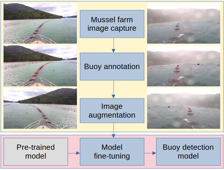
Figure 1: Raw images are collected from the cameras, which are annotated with bounding boxes around the buoys. Image augmentations are applied to the image dataset before fine-tuning the pre-trained model, resulting in our buoy detection model.

TABLE I: Training parameters

Hyperparameters		Image Augmentation
Parameter	Value	Parameter	Value
Training epochs	50	Focal loss gamma	0.0
Batch size	8	HSV-Hue	0.015
Number of workers	8	HSV-Saturation	0.7
Optimizer	SGD	HSV-Value	0.4
Initial learning rate	0.01	Rotation degrees	0.0
Final learning rate	0.01	Translation	0.1
SGD Momentum	0.937	Scale	0.5
Optimizer weight decay	0.0005	Shear	0.0
Warmup epochs	3.0	Perspective	0.0
Warmup momentum	0.8	Flip up-down prob.	0.0
Warmup bias learning rate	0.1	Flip left-right prob.	0.5
Box loss gain	0.05	Mosaic prob.	1.0
Class loss gain	0.5	Mixup prob.	0.05
Object loss gain	1.0
Anchor target threshold	4.0

III-B Mussel Farm Dataset Establishment

The image datasets used for this study were captured from three camera sources deployed differently in the mussel farm, as shown in Table II.

III-B1 Boat camera

These images are from cameras mounted on a boat. Video footage was taken while the boats were traversing the mussel farm. A random selection of frames was taken from videos. The raw frame resolution was 1920x1080 pixels. The images are typically in fine weather in the daylight, which shows high-quality image details. Row 1 in Fig. 2 shows some samples of such cases.

III-B2 Low-resolution buoy mounted camera

These images are from a camera mounted on a buoy in the mussel farm. Videos were taken in all weather conditions and all light conditions (see Fig. 2, 2nd row). A random selection of frames was taken from videos, and images that were too dark were removed. The raw frame resolution was 1920x1080 pixels.

III-B3 High-resolution buoy mounted camera

These images are from a higher-resolution camera mounted on top of a buoy in the mussel farm. Videos were taken in all weather conditions and all light conditions (see Fig. 2, 3rd row). A random selection of frames was taken from videos, filtering out images that were too dark. The raw frame resolution was 4032x3040 pixels.

The collected datasets were carefully ablated to explore their impacts on the final performance. Furthermore, an additional adverse weather test set was established from the low-resolution buoy-mounted camera source through a random selection of frames in a video where the weather was very windy, with limited visibility and rain or sea spray in the air hitting the camera (see Fig. 2, 4th row). Using it, we aim to test the robustness of our model on images with challenging in-the-wild conditions.

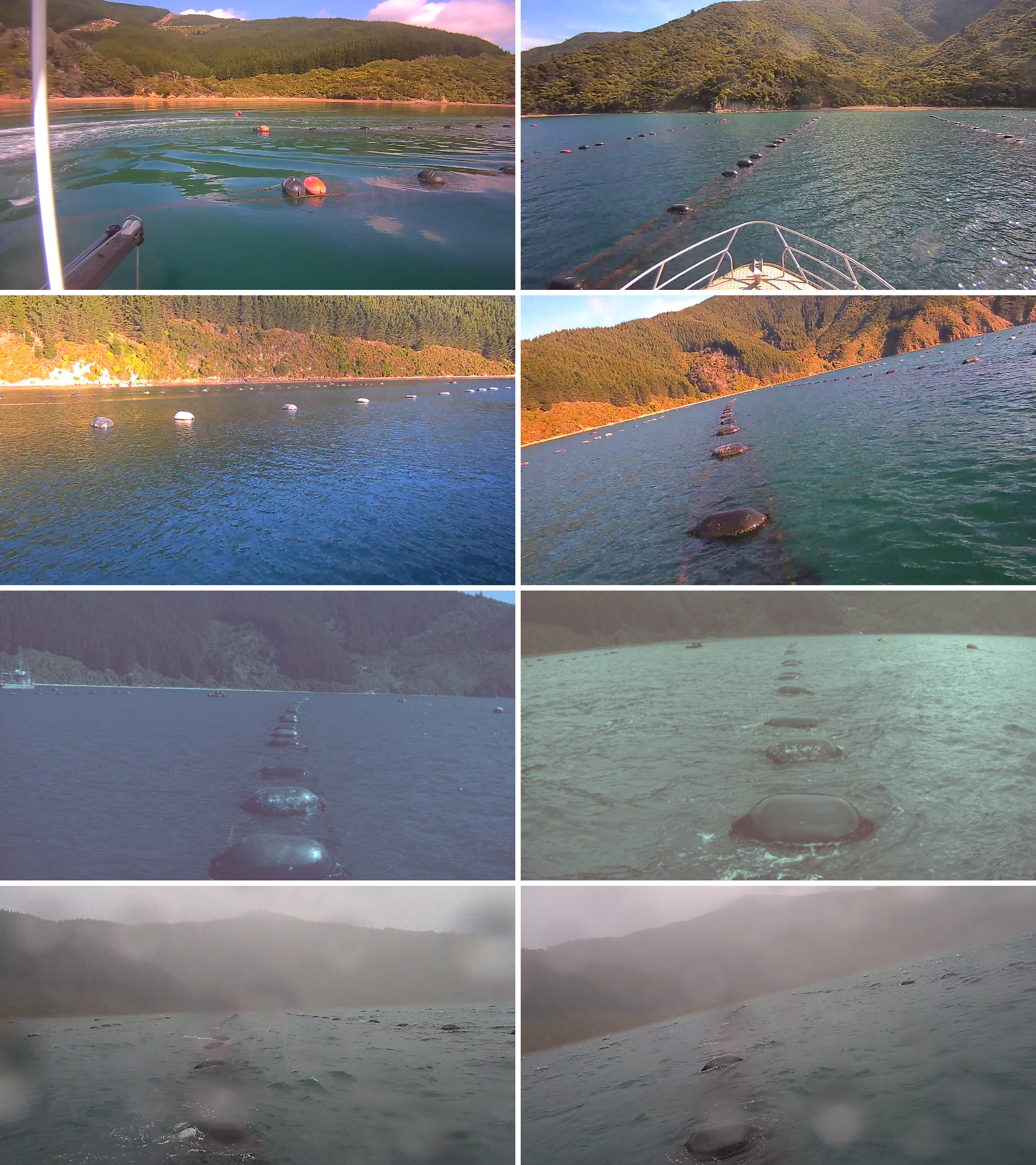
Figure 2: Image samples from dataset samples. Row 1: Boat camera. Row 2: Low-resolution buoy-mounted camera. Row 3: High-resolution buoy-mounted camera. Row 4: Low-resolution buoy-mounted camera with adverse weather.

TABLE II: Data sources

Data source	Image sample size
Boat camera	701
Buoy mounted camera (low res)	181
Buoy mounted camera (high res)	160
All Combined	1042

All dataset images were annotated with bounding boxes around the buoys that could be distinguished. All of the datasets except for the adverse weather dataset were split into training, validation, and testing datasets with a 70/10/20 ratio. The adverse weather dataset was only used for testing. The resulting dataset sizes are shown in Table III.

TABLE III: Datasets

Dataset	Train size	Validation size	Test size
Boat camera	489	70	141
Buoy mounted camera (low res)	112	16	32
Buoy mounted camera (high res)	126	18	37
All combined	728	104	209
Adverse weather	0	0	50

III-C Model fine-tune

We fine-tuned YOLOv7 and its variants [4] with mussel farm image datasets. The YOLOv7 [4] implementation was cloned from the official implementation[11]. Weights of standard YOLOv7 [12] and its tiny counterpart (YOLOv7-tiny) [13] pre-trained on the Microsoft COCO dataset [14] were used as starting points for the training of the buoy image data. We retain all the convolutional layers as the trainable layers and substitute the number of output classes per bounding box anchor to one class of buoy. All models were trained using the same hyperparameters [15] and image augmentations shown in Table I. Four variations of the models from Table IV were trained over 50 epochs each, with batch sizes of 8.

TABLE IV: Models and inputs

Name used	Input image size	Base model name	Params
tiny-640	640x640 pixels	YOLOv7-tiny	6.2M
full-640	640x640 pixels	YOLOv7	36.9M
tiny-1280	1280x1280 pixels	YOLOv7-tiny	6.2M
full-1280	1280x1280 pixels	YOLOv7	36.9M

The hardware used for training the models was the NVIDIA A100 40GB GPU partition of the VUW Rāpoi HPC cluster [16]. The hardware used for model inference was an NVIDIA GTX 1660 Ti laptop GPU because this was a less powerful GPU and would be closer to the target GPU that would be used for detection in the mussel farm.

IV Buoy Detection Experiments

IV-A Evaluation Metrics

The main metrics utilized in this study encompasses the inference frames rate, measured in frame per second (FPS), to evaluate processing speed, along with the mean average precision (mAP) to evaluate detection accuracy.

IV-A1 Inference time

Inference time is the time the inference process takes when detecting the buoys on a given image.

IV-A2 Inference FPS

Inference FPS is the number of images a model can detect buoys per second. It is the inverse of inference speed in seconds. Ideally, the inference FPS should be higher than the video FPS so that it can process videos in real-time.

IV-A3 IoU

The intersection over union (IoU) is the proportional area of overlap of two bounding boxes, normally the ground truth and prediction bounding boxes [17].

IV-A4 mAP

Mean average precision (mAP) takes the area under the precision versus recall curve, ranging from 0.5 IoU to 0.95 IoU, with increments of 0.05 steps. This is then averaged over all IoUs, and all classes, considering that there is a single class in this study - the buoy class) (referred to as mAP@[.5:.05:.95] or shortened to mAP)[17]. The mean average precision at 0.5 IoU (mAP@0.5) is more lenient in its assessment, focusing on mAP at 0.5 IoU level.

IV-B Performance of Fine-tuned Models

The results for inference time and FPS are presented in Table V, and FPS is visualised in Fig. 3. As observed, the inference FPS of the tiny-640 model was much faster than the others at about 147 FPS, and the full-1280 model was much slower at about 13 FPS. The cameras used for video on the mussel farm shoot at 15 FPS, so with the GPU used for inference, all models except for the full-1280 model could process images at a feasible real-time speed.

TABLE V: Time metrics

Model	Inference (ms)	FPS	Memory (MB)
tiny-640	6.8	147.1	972
full-640	24.5	40.8	1324
tiny-1280	16.1	62.1	1108
full-1280	75.4	13.3	1672

As shown in Table V, the maximum memory used for each model during inference varied from about 1GB for the tiny-640 model to about 1.7GB for the full-1280 model. This range of memory was affordable for the NVIDIA GTX 1660 Ti laptop GPU that was used for the on-site inference.

Table VI presents the performance metrics for each model evaluated on the all combined test set. A non-maximum suppression (NMS) IoU threshold of 0.65 and a confidence threshold of 0.001 were used as the metrics. In terms of results on mAP and mAP@0.5, the full-1280 model had the highest performance, and the tiny-640 model had the lowest performance, as would be expected. This is further illustrated in Fig. 3. The most interesting result is that the tiny-1280 model outperforms the full-640 model, which shows that increasing the input image size from 640 pixels to 1280 pixels has a more positive impact on performance than increasing the model size from YOLOv7-tiny to YOLOv7. A possible explanation for this might be that the larger image size increases the ability of both YOLOv7-tiny and YOLOv7 to pick up smaller buoys in the images, which could be lost in decreased image sizes.

TABLE VI: Performance metrics

Model	F1	Precision	Recall	mAP	mAP @0.5
tiny-640	0.579	0.684	0.502	0.237	0.569
full-640	0.726	0.823	0.649	0.378	0.748
tiny-1280	0.785	0.816	0.756	0.435	0.836
full-1280	0.865	0.890	0.841	0.554	0.908

As shown in Fig. 3, which summarises mAP, mAP@0.5, and inference FPS, we can see that out of the four models, the YOLOv7-tiny architecture with 1280px input images achieves the best balance between all of these metrics. Its performance on mAP and mAP@0.5 are slightly lower than YOLOv7 with 1280px input images but the inference FPS is much higher.

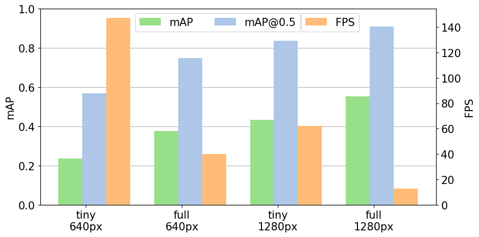
Figure 3: Each model variation shows mAP@[0.5:0.05:0.95] and mAP@0.5. Each model also shows inference FPS. Higher is better for all displayed metrics.

Detection results of each model across a range of conditions are shown in Fig. 4. As shown, all models predicted the large buoys well. What stands out is that the models using the larger 1280px images as input picked up more of the smaller buoys in the background, which is most apparent in row 1 from Fig. 4. An interesting anomaly in row 6 from Fig. 4 is that while the tiny-640 model misses a lot of the small buoys at the left of the image, at the right of the resultant image it picks up many buoys in the distance that none of the other models picked up. However, judging from the much lower mAP results in Fig. 3 for the tiny-640 model, it is probably quite a rare occurrence.

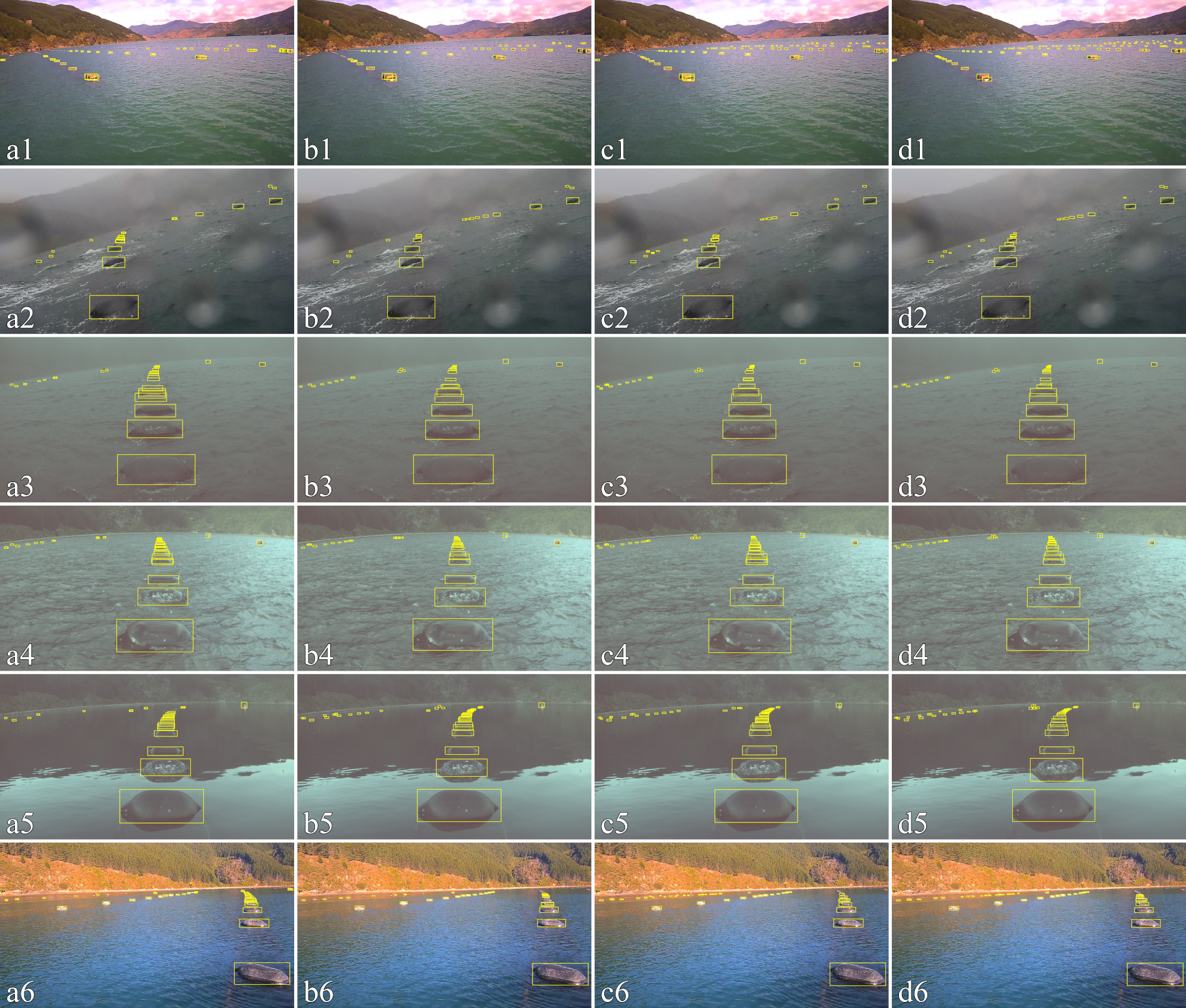
Figure 4: A different model is shown in each column: a. tiny-640, b. full-640, c. tiny-1280, d. full-1280. Various example images demonstrating a variety of scenarios are shown in each row as: 1. Many small buoys, 2. Choppy water, 3. Foggy conditions, 4. Rough conditions, 5. Calm conditions with distinct shadows on the water, 6. Calm conditions

IV-C Ablation study

The models from Table IV were trained and tested on different datasets from the different camera sources listed in Table III to see how YOLOv7 performs on such data variations. The adverse weather test set was also evaluated against all models to see how well they handled adverse weather conditions. The performance metrics for models trained and tested on the boat camera dataset, the buoy camera (high res) dataset, and the buoy camera (low res) dataset are shown in Table VII.

TABLE VII: Results for each dataset

Model	F1	Precision	Recall	mAP	mAP @0.5
Results of Boat camera trained models
tiny-640	0.675	0.791	0.588	0.332	0.667
full-640	0.667	0.769	0.589	0.324	0.655
tiny-1280	0.844	0.875	0.816	0.546	0.900
full-1280	0.843	0.877	0.812	0.542	0.898
Results of Buoy camera (high res) trained models
tiny-640	0.585	0.560	0.613	0.244	0.594
full-640	0.574	0.607	0.545	0.234	0.574
tiny-1280	0.793	0.801	0.785	0.413	0.841
full-1280	0.804	0.829	0.780	0.425	0.850
Results of Buoy camera (low res) trained models
tiny-640	0.515	0.574	0.467	0.206	0.495
full-640	0.522	0.569	0.483	0.206	0.490
tiny-1280	0.789	0.798	0.780	0.456	0.847
full-1280	0.795	0.839	0.755	0.461	0.848

In terms of mAP performance, the model trained using the boat camera images performed the best. One possible reason is the boat camera dataset has much more training data than the buoy camera-only datasets. The performance of the models trained with all combined data was better than those trained with boat camera data on the full-sized YOLOv7 architecture, but worse on the YOLOv7-tiny architecture.

The adverse weather test dataset was evaluated against all models trained with the different datasets. Results are shown in Table VIII, abbreviations HR is for high resolution, and LR is for low resolution. Results are only shown for the YOLOv7 with 1280 pixel size input (full-1280) model for brevity as results for the other models were relatively similar.

TABLE VIII: Results of Adverse weather

Dataset model was trained on	F1	Precision	Recall	mAP	mAP @0.5
Boat cam	0.545	0.685	0.453	0.298	0.501
Buoy cam (HR)	0.474	0.543	0.421	0.189	0.441
Buoy cam (LR)	0.772	0.803	0.744	0.477	0.834
All combined	0.826	0.836	0.816	0.571	0.886

In terms of mAP, performance was lower in general when evaluating the adverse weather test set against the boat camera and high-resolution buoy camera models. However, performance was relatively better against the low-resolution buoy camera models and all combined dataset models compared with other models. This was under expectation because the adverse weather test images were sampled from the same data source as the low-resolution buoy camera dataset, which is also included in the combined dataset.

Fig. 5 shows the mAP of the full-1280 models trained using each dataset, evaluated with their own test set and the adverse weather test set. For the results, we can see that the low-resolution buoy camera model and the combined model outperform the other models by a large margin when evaluated on the adverse weather test dataset.

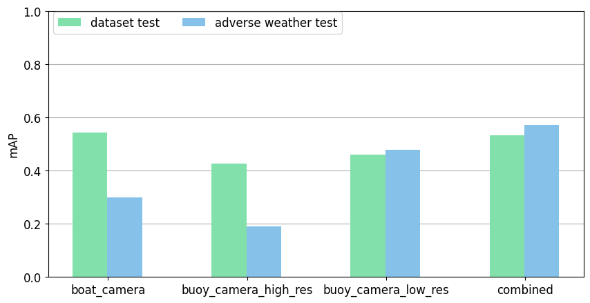
Figure 5: YOLOv7 with 1280px input model trained and tested on various datasets and also tested on the adverse weather dataset shows mAP@[0.5:0.05:0.95].

It’s noteworthy that we did not need additional preprocessing of the adverse weather images before feeding into the YOLO models as other studies [8, 9] have used before. This is because YOLOv7 has improved over YOLOv3 used in the previous studies [8, 9] for detecting objects in adverse weather conditions as reported by Haimer et al. [10].

V Conclusions and Future Work

This study successfully developed a deep learning model for buoy detection to automate the mussel farm supervision. A transfer learning-based pipeline was proposed and the effectiveness of the resultant model was exhaustively evaluated, including robustness under adverse weather conditions. The results show that the YOLOv7 model with an input image size of 1280x1280 pixels had the best performance in terms of mAP metric, while the YOLOv7-tiny model with an input image size of 1280x1280 pixels had the best balance of mAP performance and inference FPS. The models performed better on adverse weather conditions when trained with data from the same camera source.

Further work would be to accommodate the outcome of this study into real usage. These developed deep learing models could be deployed as part of an automated mussel farm monitoring pipeline for detecting drifting or sinking buoys to assist its maintenance operations. Additionally, further investigation could be on searching optimal hyperparameters and advancing image augmentations, as well as improving small object detection in sea images.

References

- [1] NZ Government Ministry for Primary Industries, “The New Zealand Government Aquaculture Strategy,” 2019.
- [2] Ying Bi, Bing Xue, Dana Briscoe, Ross Vennell, and Mengjie Zhang, “A new artificial intelligent approach to buoy detection for mussel farming,” Journal of the Royal Society of New Zealand, pp. 1–25, June 2022.
- [3] Dylon Zeng, Ivy Liu, Bi Ying, Ross Vennell, Dana Briscoe, Bing Xue, and Mengjie Zhang, “A New Multi-Object Tracking Pipeline Based on Computer Vision Techniques for Mussel Farms,” Journal of the Royal Society of New Zealand, pp. 1–20, 2023.
- [4] Chien-Yao Wang, Alexey Bochkovskiy, and Hong-Yuan Mark Liao, “YOLOv7: Trainable bag-of-freebies sets new state-of-the-art for real-time object detectors,” 2022, Publisher: arXiv Version Number: 1.
- [5] Joseph Redmon, Santosh Divvala, Ross Girshick, and Ali Farhadi, “You Only Look Once: Unified, Real-Time Object Detection,” in 2016 IEEE Conference on Computer Vision and Pattern Recognition (CVPR), Las Vegas, NV, USA, June 2016, pp. 779–788, IEEE.
- [6] Hangyue Zhao, Hongpu Zhang, and Yanyun Zhao, “YOLOv7-sea: Object Detection of Maritime UAV Images based on Improved YOLOv7,” in 2023 IEEE/CVF Winter Conference on Applications of Computer Vision Workshops (WACVW), Waikoloa, HI, USA, Jan. 2023, pp. 233–238, IEEE.
- [7] Joseph Redmon and Ali Farhadi, “YOLOv3: An Incremental Improvement,” 2018, Publisher: arXiv Version Number: 1.
- [8] Wenyu Liu, Gaofeng Ren, Runsheng Yu, Shi Guo, Jianke Zhu, and Lei Zhang, “Image-Adaptive YOLO for Object Detection in Adverse Weather Conditions,” Proceedings of the AAAI Conference on Artificial Intelligence, vol. 36, no. 2, pp. 1792–1800, June 2022.
- [9] Qingpao Qin, Kan Chang, Mengyuan Huang, and Guiqing Li, “DENet: Detection-driven Enhancement Network for Object Detection Under Adverse Weather Conditions,” in Computer Vision – ACCV 2022, Lei Wang, Juergen Gall, Tat-Jun Chin, Imari Sato, and Rama Chellappa, Eds., vol. 13843, pp. 491–507. Springer Nature Switzerland, Cham, 2023, Series Title: Lecture Notes in Computer Science.
- [10] Zineb Haimer, Khalid Mateur, Youssef Farhan, and Abdessalam Ait Madi, “YOLO Algorithms Performance Comparison for Object Detection in Adverse Weather Conditions,” in 2023 3rd International Conference on Innovative Research in Applied Science, Engineering and Technology (IRASET), Mohammedia, Morocco, May 2023, pp. 1–7, IEEE.
- [11] YOLOv7 Contributors, “Yolov7 source repository,” https://github.com/WongKinYiu/yolov7, [Online; accessed 12-June-2023].
- [12] YOLOv7 Contributors, “Yolov7 pre-trained coco weights,” https://github.com/WongKinYiu/yolov7/releases/download/v0.1/yolov7_training.pt, [Online; accessed 12-June-2023].
- [13] YOLOv7 Contributors, “Yolov7-tiny pre-trained coco weights,” https://github.com/WongKinYiu/yolov7/releases/download/v0.1/yolov7-tiny.pt, [Online; accessed 12-June-2023].
- [14] Tsung-Yi Lin, Michael Maire, Serge Belongie, Lubomir Bourdev, Ross Girshick, James Hays, Pietro Perona, Deva Ramanan, C. Lawrence Zitnick, and Piotr Dollár, “Microsoft COCO: Common Objects in Context,” 2014, Publisher: arXiv Version Number: 3.
- [15] YOLOv7 Contributors, “Yolov7 training hyperparameters,” https://github.com/WongKinYiu/yolov7/blob/main/data/hyp.scratch.tiny.yaml, [Online; accessed 12-June-2023].
- [16] VUW Research Computing Contributors, “Rāpoi - vuw’s high performance compute cluster,” https://vuw-research-computing.github.io/raapoi-docs/, [Online; accessed 15-June-2023].
- [17] Jonathan Hui, “mAP (mean Average Precision) for Object Detection,” https://jonathan-hui.medium.com/map-mean-average-precision-for-object-detection-45c121a31173, 2018, [Online; accessed 16-June-2023].