Rigorous and simple results on very slow thermalization, or quasi-localization, of the disordered quantum chain.

Abstract

This paper originates from lectures delivered at the summer school ”Fundamental Problems in Statistical Physics XV” in Bruneck, Italy, in 2021. We give a brief and limited introduction into ergodicity-breaking induced by disorder. As the title suggests, we include a simple yet rigorous and original result: For a strongly disordered quantum chain, we exhibit a full set of quasi-local quantities whose dynamics is negligible up to times of order $\exp{c(\log W)^{2-\epsilon}}$, with $\epsilon<1$, $c$ a numerical constant, and $W$ the disorder strength. Such a result, that is often referred to as ”quasi-localization”, can in principle be obtained in other systems as well, but for a disordered quantum chain, its proof is relatively short and transparent.

1 Introduction

1.1 ”Non-thermalizing” or ”ergodicity-breaking” phases

Thermalization is probably one of the most natural phenomena in the physical world. All of us know, at some level of understanding, that objects tend to exchange heat with each other until they reach the same temperature. The reason why this process is natural and, in most cases, inescapable, is because it is driven by entropy and the second law of thermodynamics. Therefore, it is also largely independent of any microscopic details, like for example the distinction classical versus quantum. It is therefore rather surprising that there exist systems where thermalization does not occur, or only after a surprisingly long time. In recent years, one tends to call this phenomenon ”ergodicity-breaking”. Obviously, lack of ergodicity is not necessarily the same as ”lack of thermalization”, but we will not elaborate on the difference here. In the present note, we take ”lack of thermalization” to mean that some local observables do not evolve towards the equilibrium value (set by the energy density of the system) at long or infinite time. Such a crude definition will suffice for us. However, for systems with multiple locally conserved quantities or with a time-dependent Hamiltonian, that definition would of course need to be refined.

The word ”phases” in the title of this subsection suggests that the lack of thermalization happens in a robust way, i.e. not resulting from any fine-tuning. We will stress the notion of robustness later on.

Finally, in the literature, the stress is mostly on lack of thermalization for infinite times (i.e. thermalization never happens), which is usually referred to as ”many-body localization” (MBL), see e.g. [1, 2, 3, 4, 5, 6, 7, 8, 9, 10, 11] for early works and [12, 13] for reviews.

This is certainly the most interesting phenomenon from a philosophical and mathematical point of view, but it might not be the most relevant phenomenon experimentally. In this note, we focus on a slightly weaker phenomenon: thermalization need not be delayed indefinitely, but simply for a time that grows faster than polynomially in some natural parameter. This is sometimes denoted as ”quasi-localization” or ”asymptotic localization” and it means that thermalization happens by processes beyond perturbation theory, see [14, 15, 16, 17, 18] for results in many-body systems at positive densities and [19, 20, 21, 22, 23, 24, 25] for stronger results and conjectures at finite energies (i.e. near the ground state if one is in a quantum setting).

The existence of genuine MBL has been debated lately [26, 27, 28, 29, 30], but the existence of ”quasi-localization” is not in doubt and it is within reach of mathematical treatment, as this article hopes to illustrate. Actually, the system that we will treat in detail - the disordered quantum chain - is a system where genuine MBL is actually expected by many authors, but we will not discuss this at all.

1.2 Partial or complete lack of thermalization

This distinction is best illustrated by examples. Imagine a system in a glassy phase. It does not thermalize to its real equilibrium state, or at least not on reasonable time-scales, but clearly some dissipative phenomena take place in a glass. In particular, there is definitely transport of heat throughout the system. This is hence an example of partial lack of thermalization. Another such example are systems with emergent conserved quantities. For concreteness, we can think of the fermionic Hubbard model in the regime where the on-site interaction $U$ is much larger than other local energy scales. In this regime, the state with two fermions at site $i$ and zero fermions at site $i+1$, has a very different energy from states where both sites $i,i+1$ host one fermion. This ”lack of resonance” will lead to a remarkable stability of sites with two fermions, also called doublons. The decay time of the doublon grows exponential in $U$ and one can introduce the doublon number as an emergent conserved quantity. This emergent conserved quantity delays proper thermalization: the system will first appear to thermalize to a state determined by total energy and total doublon number, instead of a state that is unconstrained by doublon number. This apparent thermalization to a non-equilibrium state is usually called ”prethermalization”, see [31, 32, 33, 34, 35, 36, 37, 38, 39, 40]. Therefore, also in this example, the lack of thermalization does not exclude dissipative processes. For example, the doublons can carry dissipative currents.

By complete lack of thermalization, we mean that there are no dissipative phenomena taking place (on reasonable timescales), except for dephasing and entanglement spreading. This is of course a very physical but rather vague definition. In practise, we replace it by a mathematical definition that is more precise:

Complete lack of thermalization means that there is a full set of quasi-local quasi conserved quantities, also known as quasi-LIOMs (local integrals of motion): Any operator that commutes with all these quasi-LIOMs is necessarily in the algebra generated by the quasi-LIOMs. In Section 3, we will explicitly derive absence of dissipative transport from the existence of a full set of quasi-LIOMs.

1.3 Robustness

We cannot stress too often that we are talking here about a robust phenomenon. Non-interacting spins or particles are non-thermalizing, but this is obviously not a deep or interesting observation. It becomes interesting if the absence of thermalization persists upon adding a generic small coupling between the particles or spins. Quasi-localization precisely means that the coupling between spins or particles induces thermalization and transport only non-perturbatively in the coupling strength. In our experience, the question of robustness is often overlooked when describing ergodicity-breaking. In subsection 2.3, we illustrate how easy it is to cook up non-robust models of ergodicity-breaking.

1.4 Importance of interactions

There is a huge body of literature on Anderson localization [41, 42, 43, 44] and the insulator/metal transition, a concept that was not mentioned in the above discussion. The reason is that we deal with many-body interacting systems whereas Anderson localization concerns one-particle systems, and in particular the transition between extended and localized one-particle states. From our point of view, non-interacting particles are always non-thermalizing, regardless of whether the one-particle eigenstates are localized (as in subsection 2.2) or extended (as in subsection 2.4).

2 Simple but non-robust examples

In this section, we introduce some notation and concepts, suitable for dealing with quantum spin systems. Then we list three examples of non-thermalization. We point out the similarities and crucial differences with the topic of the present article. In the terminology used in subsections 1.1 and 1.2, all three examples are examples of genuine complete lack of thermalization, but all three are non-robust.

2.1 Setup for spin chains

Let us consider a spin chain, i.e. $N$ copies of $1/2$-spins arranged on a line. The Hilbert space is ${\mathcal{H}}_{N}=({\mathbb{C}}^{2})^{\otimes_{N}}$ and we label spins or sites by $i\in\{1,\ldots,N\}$. The most general operator on ${\mathcal{H}}_{N}$ is a linear combination of operators of the form $A_{1}\otimes A_{2}\otimes\ldots\otimes A_{N}$ with $A_{i}$ acting on spin/site $i$. In practice, only local operators, i.e. operators for which all but a finite number of $A_{i}$ are equal to identity, are relevant. We will use the notation $X,Y,Z$ for the $2\times 2$ Pauli matrices $\sigma_{x},\sigma_{y},\sigma_{x}$ and we write then $X_{i},Y_{i},Z_{i}$ for copies of these matrices acting on the site $i$. It is customary to use the notation $X_{i}$ also for $\mathds{1}\otimes X_{i}\otimes\mathds{1}$, i.e. for operators acting on the full Hilbert space ${\mathcal{H}}_{N}$, but such that they act as identity on spins other than $i$. We say then that $X_{i}$ is supported in $i$, that $X_{i}Y_{j}$ is supported in $\{i,j\}$, etc. In general, the phrase “$A$ is supported on a set $S$” means that the operator $A$ can be written as a product $A_{S}\otimes\mathds{1}_{S^{c}}$ with $A_{S}$ acting on the $2^{|S|}$-dimensional space that consists of $|S|$ copies of ${\mathbb{C}}^{2}$ and $\mathds{1}_{S^{c}}$ standing for identities acting on the complement of $S$. As already said, the relevant class of observables is one that has some locality, i.e. a support consisting of a small number of sites, in particular not growing with $N$. In practice, one however cannot avoid dealing with quasi-local operators instead of purely local ones. Concretely, we will say that $A$ is $(C_{A},\kappa)$-exponentially quasi-local around some region $S$ if it can be written as

$$A=\sum_{r=0}^{\infty}A_{r},\qquad||A_{r}||\leq C_{A}e^{-\kappa r},$$ (2.1)

where $A_{r}$ is supported on $S_{r}$, the $r$-fattening of $S$, i.e.  $S_{r}=\{i|\,\mathrm{dist}(i,S)\leq r\}$ and $\norm{\cdot}$ is the operator norm $||A||=\mathop{\sup}\limits_{\psi\in{\mathcal{H}}_{N},||\psi||_{2}=1}||A\psi||_{2}$ where we wrote $||\cdot||_{2}$ for the Hilbert space norm. The Hamiltonians $H$ that we consider will be sums $H=\sum_{i}H_{i}$ where the local terms $H_{i}$ are exponentially quasi-local around the respective sites $i$. Of course, one could consider a weaker notion of quasilocality, allowing for example interactions that decay like a power law, but for simplicity we restrict to the exponentially quasi-local setup. Insightful reviews on the above setup can be found for example in [45, 46].

2.2 Uncoupled spins: the trivial case

Consider the Hamiltonian

$$H_{0}=h\sum_{i=1}^{N}Z_{i}.$$ (2.2)

This Hamiltonian describes free, i.e. non-interacting, spins. It is clear that this model does not thermalize, as each of the operators $Z_{i}$ is a conserved quantity, i.e.

$$\derivative{t}Z_{i}={{\mathrm{i}}}[H_{0},Z_{i}]=0.$$ (2.3)

This means that, whatever profile of energy we impose on the system at the initial time, this profile will be exactly conserved in time. More precisely, let the initial wavefunction be $\Psi_{0}$ and the time-evolved wavefunction $\Psi_{t}=e^{-{{\mathrm{i}}}tH_{0}}\Psi_{0}$, then the energy profile

$$E_{i}(t)=\langle\Psi_{t}|hZ_{i}|\Psi_{t}\rangle$$

is actually independent of time $t$. In particular, there is no flow of energy from high to low energy densities.

2.3 Uncoupled spins in disguise: dressing transformation

We now introduce $A$ to be an arbitrary short-ranged Hamiltonian of the form $A=\sum_{i}A_{i}$ with $A_{i}$ local terms supported in the vicinity of $i$. Then, let us define the Hamiltonian as the Heisenberg evolution generated by $A$ and up to a finite time $s$, of the trivial Hamiltonian $H_{0}$ introduced in (2.2):

$$H_{1}=e^{{{\mathrm{i}}}sA}H_{0}e^{-{{\mathrm{i}}}sA}=\sum_{i}h\tau_{i},\qquad\tau_{i}=e^{{{\mathrm{i}}}sA}Z_{i}e^{-{{\mathrm{i}}}sA}.$$

First, we should convince ourselves that $H_{1}$ is actually a bonafide Hamiltonian as defined in subsection 2.1. Indeed, the Lieb-Robinson bound (discussed below, see e.g. Lemma 7.2) ensures that $\tau_{i}=e^{{\mathrm{i}}sA}Z_{i}e^{-{\mathrm{i}}sA}$ is exponentially quasi-local around site $i$. We could write each of the $\tau_{i}$ as a sum of local terms, as in (2.1). If one was presented the operators $\tau_{i}$ and $H_{1}$ in such a form, one would probably not see anything special about them. It would just be a hopelessly complicated Hamiltonian. However, the above definition of $\tau_{i}$ and $H_{1}$ reveals of course a very special property: all these operators $\tau_{i}$ are mutually commuting, because

$$[\tau_{i},\tau_{j}]=[e^{{{\mathrm{i}}}sA}Z_{i}e^{-{{\mathrm{i}}}sA},e^{{{\mathrm{i}}}sA}Z_{j}e^{-{{\mathrm{i}}}sA}]=e^{{{\mathrm{i}}}sA}[Z_{i},Z_{j}]e^{-{{\mathrm{i}}}sA}=0.$$

Consequently, since $H_{1}=\sum_{i}h\tau_{i}$, we have

$$[H_{1},\tau_{i}]=0,$$

similar to what we had in the trivial example (2.3), with the only difference that the $\tau_{i}$ are exponentially quasi-local, rather than strictly local. Of course, all of this could have been guessed from the start: $H_{1}$ just describes uncoupled spins in disguise.

2.4 Integrable systems

Let us now consider the transverse Ising chain

$$H_{2}=\sum_{i=1}^{N}hZ_{i}+\sum_{i=1}^{N-1}JX_{i}X_{i+1}.$$

This Hamiltonian is not of the type considered in subsection 2.3, but it has another special property. It can be mapped via a unitary transformation $U$ (the Jordan Wigner transformation combined with Fourier transform) to non-interacting fermions

$$UH_{2}U^{*}=\sum_{k\in\mathbb{T}_{N}}\omega(k)c^{\dagger}_{k}c_{k},\qquad\mathbb{T}_{N}=\frac{2\pi}{N}\times\{1,\ldots,N\},$$

for some set of operators $c_{k},c^{\dagger}_{k}$ that satisfy the fermionic commutation relations

$$\{c_{k},c^{\dagger}_{k^{\prime}}\}=\delta_{k,k^{\prime}},\qquad\{c_{k},c_{k^{\prime}}\}=\{c^{\dagger}_{k},c^{\dagger}_{k^{\prime}}\}=0,$$

and some function $\omega$, that is interpreted as the dispersion relation of the fermionic modes with momentum $k$. We see again that there is a sense of non-thermalization here. The occupation numbers $n_{k}=c^{\dagger}_{k}c_{k}$ are conserved: $[H_{2},n_{k}]=0$. If we start out with only the right-moving fermion modes (i.e. those with $\partial_{k}\omega(k)\geq 0$), then this will stay so forever. Again the model has $N$ meaningful (cf. the discussion in subsection 2.5) and independent conserved quantities, which prohibit thermalization. One usually refers to models like $H_{2}$ as being ”integrable” and, whereas this model is also ”non-interacting”, this need not be the case. The study of integrable models is rich and interesting, but we will not pursue it here.

2.5 (Quasi-)locality of conserved quantities

In all three of the examples above, we identified $N$ conserved, independent quantities. What is so special about this? After all, in general a Hamiltonian $H$ on ${\mathcal{H}}_{N}$ is a large matrix that can always be diagonalized by some unitary $U$, and this always provides us with an algebra of conserved quantities (containing in particular the spectral projections of $H$). However, the crucial point in the three examples above, is that the conserved quantities have some form of locality. In the first example they are strictly local and in the second example they are exponentially quasi-local. The third example is a bit of an outlier since the mapping from spins to fermions is itself non-local. However, the concerned quantities are sums of local operators in the fermion representation, which is still a meaningful notion of locality.
More importantly, in all these three examples, the conserved quantities provide us with physically meaningful constraints on the evolution of the system. This should be contrasted with a generic system, where conserved quantities like spectral projections do not have any sense of locality and therefore do not give any practically observable constraints on the time evolution.

2.6 Fragility of the three examples

None of the three examples described above are robust. If one adds a small arbitrary perturbation to the Hamiltonian, the described phenomenon disappears. By a small perturbation, we could for example mean that

$$H\rightarrow H+\epsilon P,\qquad P=\sum_{i}P_{i},\qquad\epsilon\ll 1,$$

with each $P_{i}$ exponentially quasi-local around $i$. For the examples of subsections 2.2 and 2.3, the perturbed systems retain a partial lack of thermalisation. Namely, there will be a single emergent quasi-conserved quantity corresponding to the original unperturbed Hamiltonians, completely analogous to the doublon number conservation described in subsection 1.2. We do not explain this further but we refer to [35]. In the example of subsection 2.4, we have weakly broken integrability. There is no lack of thermalization remaining, according to our definition. Unfortunately, due to the history of the subject, it is precisely in weakly perturbed integrable systems, i.e. perturbation of the example from subsection 2.4, that the term ”prethermalization” has become widely known, see e.g.  [47, 48, 49, 50]. In that context, one means by this, among other things, that approach to genuine equilibrium becomes visible on time scales that appear long in comparison to other time-scales in the system (in particular, timescales governing the prethermalization to a non-equilibrium state). However, that timescale on which genuine equilibration becomes visible is still no longer than of order $1/\epsilon^{2}$, whereas the present article focuses on timescales that are superpolynomial in $1/\epsilon$. Therefore, the phenomenology of a weakly broken Hamiltonian of subsection 2.4 has very little overlap with the topic of the present article, see [51] for a recent review.

3 Results

We come to the disordered chain, the main topic of this note. Its Hamiltonian is

$$H=\sum_{i=1}^{N}\left(h_{i}Z_{i}+JV_{i}\right),$$

where the $h_{i}$ are i.i.d. (independent, identically distributed) random numbers drawn uniformly from the unit interval $[0,1]$ and $V_{i}$ are local operators whose support is contained in the discrete interval $[i,i+R-1]$, for some fixed range $R$. We write

$$H=H_{0}+JV,\qquad H_{0}=\sum_{i}h_{i}Z_{i},\qquad V=\sum_{i}V_{i},$$

and we will take $0<J\ll 1$. Without loss of generality we can then assume that $||V_{i}||\leq 1$.

3.1 Quasi-conserved quantities

The goal of our analysis is to find a full set of $N$ quantities $\tau_{i}$ that are conserved for superpolynomial time in $1/J$ and such that most of them are exponentially quasi-local around a single site. Our main results is

Theorem 3.1 (Quasi-Localization with superpolynomial lifetime).

Let the range parameter $R$, introduced above, be fixed, and choose two parameters $\beta,\epsilon\in(0,1)$. Then, there is a $J_{*}>0$ depending on those parameters $R,\beta,\epsilon$ but not on $N$, such that, for $J\leq J_{*}$, we can construct $N$ quasi-conserved operators (also known as quasi-LIOMs) $\tau_{i=1,\ldots N}$ with the properties listed below. Set

$$n_{*}=\left\lfloor(\log(1/J))^{1-\epsilon}\right\rfloor.$$ (3.1)

1. The $\tau_{i}$ are spin-operators in the sense that they are unitarily equivalent to the operators $Z_{j}$

2. They are mutually commuting: $[\tau_{i^{\prime}},\tau_{i}]=0$ for all $i,i^{\prime}$.

3. They have the following locality property: for each $i$, there is an interval $M_{i}$ containing site $i$ such that $\tau_{i}$ is $(|M_{i}|,\frac{1-\beta}{4R}\log(1/J))$- exponentially quasi-local around the interval $M_{i}$. We call the resonant set ${\mathfrak{R}}$ the set of sites $i$ for which $|M_{i}|>1$.

4. They are quasi-conserved:

   $$||[H,\tau_{i}]||\leq|M_{i}|e^{-\frac{1-\beta}{4}\log(\frac{1}{J})^{2-\epsilon}}.$$

5. They form a maximal commutative sub-algebra: Any operator commuting with all $\tau_{i}$, is itself contained in the algebra generated by the $\tau_{i}$.

6. The event $i\in{\mathfrak{R}}$ depends only on the random variables $h_{j}$ with $j\in[i-2n_{*}R+1,i+2n_{*}R-1]$, and its probability is bounded as

   $$\mathrm{Prob}(i\in{\mathfrak{R}})\leq J^{\beta/2}.$$

7. If $|M_{j}|>1$, then all sites $i$ satisfying $\mathrm{dist}(i,M_{j}^{c})\geq n_{*}R$ are elements of ${\mathfrak{R}}$. We obtain the bound

   $$\mathrm{Prob}(|M_{j}|\geq\ell)\leq e^{-\frac{\beta}{10R}(\log(1/J))^{\epsilon}\ell}.$$

As already argued in subsection 2.5, the locality property of the $\tau_{i}$-operators is crucial. In its absence, the above result is trivial. The weaker quasi-conservation property

$$||[H,Z_{i}]||\leq CJ,$$

i.e. choosing simply $\tau_{i}=Z_{i}$, follows immediately from the form of the Hamiltonian. It simply reflects that the spin flipping term is of order $J$. In some sense, the merit of the theorem is to find dressed spin operators such that terms flipping these dressed spins, are of much lower order.
To get the result in the form announced in the abstract, we can observe that from the item 4. it follows that

$$||\tau_{i}(t)-\tau_{i}(0)||\leq\int_{0}^{t}{\mathrm{d}}s\,\norm{\derivative{s}\tau_{i}(s)}=\int_{0}^{t}{\mathrm{d}}s\,\norm{[H,\tau_{i}(s)]}\leq t|M_{i}|e^{-\frac{1-\beta}{4}\log(\frac{1}{J})^{2-\epsilon}}.$$ (3.2)

Trading the parameter $J$ for the disorder strength $W$, by a simple scaling argument, we get a timescale of order $e^{c(\log W)^{2-\epsilon}}$, where we used that $|M_{i}|$ is a random variable that is typically of order 1, see item 7. It is interesting to compare this result with the paper [15]. The latter paper exhibits a timescale of order $e^{c(\log W)^{3}}$ for a chain of classical anharmonic disordered oscillators. Indeed, as already stressed, the result in Theorem 3.1 is not specific to disordered quantum systems. In some earlier papers, we derived related results for classical systems and disorder-free systems, see [16, 17, 18]. However, in all these cases, the proofs were considerably more involved compared to the present paper, and the results were slightly weaker.

3.2 Slowness of transport

The above theorem on quasi-conserved quantities is in some sense the purest characterization of ergodicity-breaking phases. Yet, from a practical point of view, the slowness of transport is probably a more intuitive statement, so let us set the scene for that. Given a fiducial site $i_{*}$, we can define a naive left-right splitting of the Hamiltonian

$$H=H_{L}+H_{R}$$

by

$$H_{L}=\sum_{i\leq i_{*}}(h_{i}Z_{i}+JV_{i}),\qquad H_{R}=H-H_{L}.$$ (3.3)

The energy current from the left region $\{i\,|\,i\leq i_{*}\}$ to the right region $\{i\,|\,i>i_{*}\}$ can be defined as

$$J_{E}={\mathrm{i}}[H,H_{L}]=-{\mathrm{i}}[H,H_{R}].$$

In general, there is no reason why this current operator would be smaller than of order $J$. Indeed, even if the system was perfectly localized, i.e. the quasi-LIOMs $\tau_{i}$ were conserved exactly, then still $J_{E}$ would detect the oscillatory motion within the LIOMs, because the nearby LIOMs have support that significantly intersects both the left region $\{i\,|\,i\leq i_{*}\}$ and the right region $\{i\,|\,i>i_{*}\}$, see Figure 1.

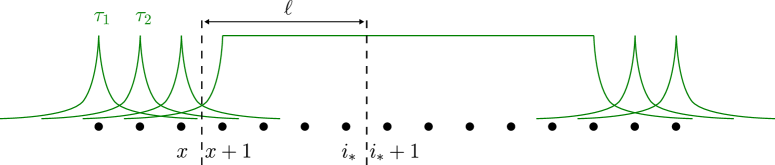
Figure 1: We represent LIOMs by drawing their peaked local structure. There are LIOMs with large spatial extent at site $i_{*}$, i.e. the interval $M_{i_{*}}$ is large. Therefore, to exhibit the smallness of time-integrated currents, we cut the system between sites $x$ and $x+1$, a distance $\ell$ from $i_{*}$. This results in a larger observable $O$ in Theorem 3.2.

Such purely oscillatory currents are not persistent, i.e. their time integral does not grow in time. To make this precise, we exhibit that the current $J_{E}$ is mostly of the form ${\mathrm{i}}[H,O]$ for some bounded observable $O$ that is quasi-exponentially local around $i_{*}$ or around a short interval containing $i_{*}$. If $J_{E}$ was exactly of this form, we would obtain

$$\int_{0}^{t}dsJ_{E}(s)=O(s)-O(0),$$ (3.4)

with $J_{E}(s),O(s),O(0)$ referring to the Heisenberg evolution. Since the right-hand side is bounded in norm by $2||O||$, then we see that such a time-integrated current is bounded uniformly in time, uniformly in the total size of the system. Note that it was important that $O$ has a norm that does itself not scale with the system size. In particular we could not have done this argument based on the expression $J_{E}={\mathrm{i}}[H,H_{L}]$ as $H_{L}$ has a norm proportional to the system size.

The following theorem captures a somewhat less perfect version of this scenario, implying that the time-integrated current $\int_{0}^{t}dsJ_{E}(s)$ is the sum of a term that is bounded uniformly in time, as in (3.4), and a term that can grow in time, but only at a very small rate, namely the bound on the commutator in Theorem 3.2. The presence of this very small rate reflects the fact that we do not show localization for infinite times.

Theorem 3.2 (Slow transport).

Let parameter $J_{*}$ be as in Theorem 3.1. For any $J\leq J_{*}$, there is an observable $O$, such that

$$||J_{E}-{\mathrm{i}}[H,O]||\leq e^{-\frac{1-\beta}{4}(\log(1/J))^{2-\epsilon}},$$

such that $||O||\leq J^{\frac{1-\beta}{8R}}+2\ell$. Here $\ell$ is a random natural number satisfying the bound

$$\mathrm{Prob}(\ell\geq\ell_{0})\leq e^{-c_{0}(\log(1/J))^{\epsilon}\ell_{0}},\qquad c_{0}=10^{-3}\beta/R.$$

Let us comment on the interpretation of random size of the observable $O$. This size reflects the extent of the quasi-LIOMs at or around the site $i_{*}$, or, in simpler terms, the quality of the localization around site $i_{*}$. Indeed, if the chain has anomalously weak disorder in a region $I$ with $I\ni i_{*}$, then, roughly speaking, $O$ is simply the sum of Hamiltonian terms between site $i_{*}$ and the nearest end of the interval $I$, a distance $\ell$ away from $i_{*}$, see Figure 1.

In the remainder of this paper, we give the proof of the the above results. First, in Section 4 we present a simplified version of the proof and then, in Sections 5,6,7 the proper proof.

4 Cartoon of the proof

The proof is inspired by the seminal work [10], but since the goal is easier, we need only the very simplest elements of that method, and none of the subtleties that render [10] difficult. From a wider perspective, the method is also known as KAM transformations, often used in classical physics. One could also call it a version of Schrieffer-Wolf transformations. In the present section, we present a toy version of the proof, with some details missing, and leading to a weakened version of Theorem 3.1.

4.1 Perturbative transformation

We follow closely the exposition given in [52]. The rough idea (that will have to be modified later on) is to look for the transformation $U=e^{A}$ with $A=\sum_{i}A_{i}$ a sum of exponentially quasi-local anti-Hermitian terms, such that

$$H^{\prime}=e^{\mathrm{ad}_{A}}H=e^{A}He^{-A}$$

is a sum of exponentially quasi-local terms that are moreover diagonal in the basis of $Z_{j}$. That is, in some sense, we anticipate that the disordered model is similar to the example in subsection 2.3. We look for such $A$ order-by-order in $J$. In this first step, we anticipate that $A$ is first order in $J$, so expansion in powers of $J$ is the same as expansion in powers of $A$. We expand, singling out zeroth and first order in $J$:

$$H^{\prime}=e^{\mathrm{ad}_{A}}H=H+[A,H]+\sum_{n=2}\frac{1}{n!}(\mathrm{ad}_{A})^{n}(H),$$ (4.1)

where we wrote $\mathrm{ad}_{A}$ for the superoperator $\mathrm{ad}_{A}=[A,\cdot]$ acting on operators. The perturbation $JV$ is first order in $J$, and we wish to reduce it to second order in $J$. Therefore, the sum $\sum_{n=2}^{\infty}\ldots$ is for the moment already small enough and we focus on $H+[A,H]$ which we rewrite as

$$H_{0}+JV+[A,H_{0}]+J[A,V]=H_{0}+\left(JV+[A,H_{0}]\right)+J[A,V].$$

In the last expression $H_{0}$ is zeroth order, and $J[A,V]$ is second order. The expression between brackets is first order and it is this expression that we want to eliminate by a judicious choice of $A$, i.e. we look for a solution of the elimination equation

$$JV+[A,H_{0}]=0.$$

Moreover, the solution $A$ should

1. be a sum of local terms $A_{i}$,

2. such that all these terms have strength of at most order $O(J)$, i.e. $||A_{i}||\leq CJ$.

If the first condition is not satisfied, then the new Hamiltonian $H^{\prime}=e^{\mathrm{ad}_{A}}H$ has no local structure, and it becomes useless (see the discussion in subsection 2.5). If the second condition is not satisfied, then the book-keeping above is no longer correct.

Finding $A$ involves finding a local inverse to the superoperator $\mathrm{ad}_{H_{0}}$. This can be done since $H_{0}$ is a sum of local commuting terms: Let $\sigma\in\{-1,1\}^{N}$ label the eigenvectors of $(Z_{j})_{j=1,\ldots,N}$, hence of $H_{0}$. They are of the form

$$|\sigma\rangle=\otimes_{i=1}^{N}|\sigma_{i}\rangle,$$

where $\ket{1},\ket{-1}$ stand for the $\pm 1$-eigenvectors of $Z$, in other words for the spin-up/spin-down states, such that

$$Z_{i}|\sigma\rangle=\sigma_{i}|\sigma\rangle.$$

Now we can find $A$ by writing

$$\langle\sigma|A|\sigma^{\prime}\rangle=\frac{J\langle\sigma|V|\sigma^{\prime}\rangle}{E(\sigma)-E(\sigma^{\prime})}\left(1-\delta_{\sigma\sigma^{\prime}}\right),$$ (4.2)

where $E(\sigma)=\langle\sigma|H_{0}|\sigma\rangle$. The factor $\left(1-\delta_{\sigma\sigma^{\prime}}\right)$ ensures that $A$ vanishes on the diagonal. This solution manifestly satisfies locality. For the sake of explicitness, we pick now a specific form for $V_{i}$:

$$V_{i}=X_{i}+X_{i}X_{i+1},$$

and we write $A$ as a sum of local terms:

$$A=\sum_{i}A_{i},\quad\langle\sigma|A_{i}|\sigma^{\prime}\rangle=\frac{J\langle\sigma|V_{i}|\sigma^{\prime}\rangle}{E(\sigma)-E(\sigma^{\prime})}\left(1-\delta_{\sigma\sigma^{\prime}}\right).$$ (4.3)

Obviously, the right-hand side of (4.3) is then nonzero only for $\sigma,\sigma^{\prime}$ that coincide on all sites except for the sites $i,i+1$, and this property is then inherited by the left-hand side. This is precisely what we mean by locality. Hence condition $i)$ above is manifestly satisfied. However, condition $ii)$ can fail if the denominator is too small. For ease of writing, let us denote by $\sigma^{i}$ the configuration $\sigma$ flipped at site $i$, i.e. with the value (spin) flipped at site $i$, i.e. such that $X_{i}|\sigma\rangle=|\sigma^{i}\rangle$. Similarly, let $\sigma^{i,j}$ be $\sigma$ flipped at both sites $i,j$. The choices of $\sigma,\sigma^{\prime}$ for which $\langle\sigma|V_{i}|\sigma^{\prime}\rangle$ does not vanish are then

$$\sigma^{\prime}=\sigma^{i}\qquad\text{and}\qquad\sigma^{\prime}=\sigma^{i,i+1}.$$

These lead to the denominators

$$E(\sigma)-E(\sigma^{i})=\pm 2h_{i}\qquad\text{and}\qquad E(\sigma)-E(\sigma^{i,i+1})=\pm 2h_{i}\pm 2h_{i+1},$$

where the choice of $+/-$ depends on $\sigma$. If we place a fixed lower bound, say $\delta$, on $|E(\sigma)-E(\sigma^{\prime})|$, then it is clear that we cannot expect this to be satisfied everywhere, i.e. for every $i$. The best we can ask for is that such a non-resonance condition

$$|E(\sigma)-E(\sigma^{\prime})|\geq\delta$$ (4.4)

is satisfied at most places in the chain, i.e. for most $i$, with $\sigma^{\prime}$ as above. The non-resonance condition holds for site $i$ iff

$$2h_{i}\geq\delta\qquad\text{and}\qquad|2h_{i}-2h_{i+1}|\geq\delta.$$ (4.5)

We say that the interval $[i,i+1]$ is resonant if (4.5) is violated. The probability that a given interval $[i,i+1]$ is resonant is clearly bounded by $C\delta$. In what follows, we do not want to treat $\delta$ simply as a small constant $c$ and we prefer to think of it as coupled to $J$ as $\delta=J^{\beta}$ with $0<\beta<1$, but for clarity and overview we will still keep different symbols. In any case, since $\delta$ is not a mere constant, we need to revise the condition $ii)$ above to read

1. All terms in $A$ have strength at most $CJ/\delta$.

However, we still face the problem that, on average, a fraction of order $C\delta$ of sites will violate the non-resonance condition (4.5). We address this issue now.

Figure 2: Illustration of resonances. The red horizontal bars denote sites that are resonant because the corresponding fields violate (4.5). By our conventions, we declare the full support of a term $V_{i}$ resonant, i.e. the pair $(i,i+1)$, as indicated at the bottom of the figure.

4.2 Treatment of resonant regions

We have to exclude resonant terms $V_{i}$, corresponding to resonant intervals $[i,i+1]$, from our procedure and so we split

$$V=V^{\cancel{{\mathfrak{R}}}}+V^{{\mathfrak{R}}},\qquad V^{\cancel{{\mathfrak{R}}}}=\sum_{i:\,[i,i+1]\,\text{non-resonant}}V_{i},\qquad V^{{\mathfrak{R}}}=\sum_{i:\,[i,i+1]\,\text{resonant}}V_{i}.$$

Instead of defining $A$ by the condition (4.2), we now define it as $A=\sum_{i\in\cancel{{\mathfrak{R}}}}A_{i}$ with

$$\langle\sigma|A_{i}|\sigma^{\prime}\rangle=\frac{J\langle\sigma|V_{i}|\sigma^{\prime}\rangle}{E(\sigma)-E(\sigma^{\prime})}\left(1-\delta_{\sigma\sigma^{\prime}}\right),\qquad i\in\cancel{{\mathfrak{R}}},$$

i.e. the definition applies only to non-resonant sites $i$. We then have

$$H^{\prime}=e^{\mathrm{ad}_{A}}H=H_{0}+JV^{\mathfrak{R}}+(JV^{\cancel{{\mathfrak{R}}}}+[A,H_{0}])+J[A,V]+\sum_{n=2}\frac{1}{n!}(\mathrm{ad}_{A})^{n}(H),$$ (4.6)

and the choice of $A$ is now such that the term between brackets vanishes. This means that we have obtained

$$H^{\prime}=H_{0}+JV^{{\mathfrak{R}}}+J^{2}V^{(2)}+\text{higher order terms in $J$},$$ (4.7)

with

$$J^{2}V^{(2)}=J[A,V]+\frac{1}{2}(\mathrm{ad}_{A})^{2}(H)=J[A,V^{{\mathfrak{R}}}]+\frac{J}{2}[A,V^{\cancel{{\mathfrak{R}}}}],$$

where the last equality follows by the definition of $A$. A little thought shows that $J^{2}V^{(2)}$ is a sum of local terms supported on 3 consecutive sites, and with strength $CJ^{2}/\delta$, i.e.

$$V^{(2)}=\sum_{i}V^{(2)}_{i},\qquad||V^{(2)}_{i}||\leq C/\delta,\qquad V^{(2)}_{i}\text{ supported on }(i,i+1,i+2).$$

The higher order terms in (4.7) have larger support, and we will need to keep track of this. However, in the next subsection 4.3, we will for simplicity disregard these terms. Taking them into account would not invalidate any of the bounds exhibited below (it can be absorbed by the constants $C$ that we write).

4.3 Construction of quasi-LIOMs

Let us take stock of what we achieved by the transformation $H\mapsto H^{\prime}$, i.e. what we can say about slowness of transport and thermalization of the Hamiltonians $H^{\prime}$ and $H$.

We argue that we have obtained a toy-version of Theorem 3.1, but instead of superpolynomial lifetime of the quasi-LIOMs, we have a polynomial lifetime, as we will exhibit below.

Above, we identified resonant intervals $[i,i+1]$. We now additionally define the resonant set of sites ${\mathfrak{R}}$ as the union of all the resonant intervals. We partition ${\mathfrak{R}}$ into intervals by the following connectedness property: We draw an edge between adjacent elements $i,i+1$ of ${\mathfrak{R}}$ whenever the interval $[i,i+1]$ is resonant. This defines a graph on ${\mathfrak{R}}$ and we call the connected components of this graph $T_{\alpha}$, for an abstract index $\alpha$. Note that necessarily $|T_{\alpha}|\geq 2$. The point of this construction is the following: For each $\alpha$, we can define operators ${\mathcal{E}}_{\alpha}$ as

$${\mathcal{E}}_{\alpha}=\sum_{i\in T_{\alpha}}h_{i}Z_{i}+J\sum_{i:\{i,i+1\}\subset T_{\alpha}}V^{{\mathfrak{R}}}_{i}$$

having the following properties:

1. $H^{\prime}=\sum_{i:i\not\in{\mathfrak{R}}}h_{i}Z_{i}+\sum_{\alpha}{\mathcal{E}}_{\alpha}+J^{2}V^{(2)},$

2. $[{\mathcal{E}}_{\alpha},{\mathcal{E}}_{\alpha^{\prime}}]=0$, and $[Z_{i},{\mathcal{E}}_{\alpha}]=0$, for $i\not\in{\mathfrak{R}}$,

3. $[{\mathcal{E}}_{\alpha},H^{\prime}]=J^{2}[{\mathcal{E}}_{\alpha},V^{(2)}]$, and $[Z_{i},H^{\prime}]=J^{2}[Z_{i},V^{(2)}]$, for $i\not\in{\mathfrak{R}}$.

Indeed, the first two properties follow easily from the above construction. Using these properties, and the fact that $[{\mathcal{E}}_{\alpha},Z_{i}]=0$ for $i\not\in{\mathfrak{R}}$, implies the third property. We then also deduce

$$||[{\mathcal{E}}_{\alpha},H^{\prime}]|| \leq 2J^{2}||{\mathcal{E}}_{\alpha}||\sum_{j:[j,j+2]\cap T_{\alpha}\neq\emptyset}||V^{(2)}_{j}||\leq C|T_{\alpha}|\frac{J^{2}}{\delta}||{\mathcal{E}}_{\alpha}||,$$ (4.8)

$$||[Z_{i},H^{\prime}]|| \leq 2J^{2}||Z_{i}||\sum_{j:[j,j+2]\ni i}||V^{(2)}_{j}||\leq C\frac{J^{2}}{\delta},\qquad i\not\in{\mathfrak{R}}.$$ (4.9)

This shows that the operators ${\mathcal{E}}_{\alpha},Z_{i}$ for $i\not\in{\mathfrak{R}}$ are quasi-conserved w.r.t. to the transformed Hamiltonian $H^{\prime}$, at least for a longer time than one would naively infer from the original Hamiltonian. However, for the moment, the number of these quantities is smaller than $N$, so this is not yet a full set of maximal quasi-conserved quantities. We remedy this now.

Fix $\alpha$ and recall that ${\mathcal{E}}_{\alpha}$ is supported on $T_{\alpha}$. We therefore identify ${\mathcal{E}}_{\alpha}$ with a local operator acting on a $d$-dimensional space, with $d=2^{|T_{\alpha}|}$. By diagonalizing this operator, one can construct $|T_{\alpha}|$ mutually commuting spin-operators (in the sense of Theorem 3.1) $\tau^{\prime}_{\alpha,j},j=1,\ldots,|T_{\alpha}|$ such that $[\tau^{\prime}_{\alpha,j},\tau^{\prime}_{\alpha}]=0$ and such that $\tau^{\prime}_{\alpha,j}$ are supported on the interval $T_{\alpha}$ as well. The labelling by $j$ is arbitrary. We now set

$$\tau^{\prime}_{i}=\begin{cases}Z_{i}&i\not\in{\mathfrak{R}}\\ \tau^{\prime}_{\alpha,j}&i\in T_{\alpha},\quad|T_{\alpha}|>1,\quad i=\min T_{\alpha}+j-1\end{cases}$$ (4.10)

obtaining a set of $N$ spin-operators.

For convenience, and to increase the similarity to Theorem 3.1, we now associate to every $\tau_{i}^{\prime}$ an interval $M_{i}$. If $i\in{\mathfrak{R}}$, then we set $M_{i}=T_{\alpha}$ and for $i\not\in{\mathfrak{R}}$, we simply take $M_{i}=\{i\}$. With these definitions, the spin operator $\tau_{i}^{\prime}$ is supported on $M_{i}$.

Proceeding now as in the derivation of (4.8) and using that now $\tau^{\prime}_{i}$ have unit norm, we obtain

$$||[\tau^{\prime}_{i},H^{{}^{\prime}}]||\leq C|M_{i}|\frac{J^{2}}{\delta}.$$ (4.11)

Since the majority of sites are non-resonant, most of the intervals $M_{i}$ above contain a single site. In contrast, how likely is it that a given site $i$ is the first left-most site of an interval $T_{\alpha}$ with large length $L$? For that to happen, the intervals $[j,j+1]$, for $j=i,\ldots,i+L-2$, all need to be resonant. The probability that one of these intervals is resonant, is bounded by $C\delta$. Since, for a given interval $[j,j+1]$, the resonance condition depends only on $h_{j},h_{j+1}$, the resonance conditions are independent whenever the intervals are disjoint. Therefore, the probability that $i$ is the left-most site of $T_{\alpha}$ with $|T_{\alpha}|=L$, is bounded by $(C\delta)^{L/2}$. The picture that emerges is that long intervals $T_{\alpha}$ are exponentially sparse.

Finally, we note that the constructed quantities are almost conserved with respect to $H^{\prime}$ and not with respect to $H$, but this is of course fixed by undoing the dressing transformation and setting

$$\tau_{i}=e^{-\mathrm{ad}_{A}}\tau^{\prime}_{i}.$$

By the Lieb-Robinson bound (discussed below, see e.g. Lemma 7.2), this transformation does not spoil the exponential quasi-locality properties. Also, since the transformation $e^{-\mathrm{ad}_{A}}$ preserves norms and products, we obtain from (4.11) that

$$||[\tau_{i},H]||=||[\tau^{\prime}_{i},H^{{}^{\prime}}]||\leq C|M_{i}|\frac{J^{2}}{\delta}.$$

This completes the first step of our procedure. We started with the operators $Z_{i}$, that were conserved up to time of order $1/J$, because $||[H,Z_{i}]||\leq CJ$, and we obtained operators $\tau_{i}$, that are conserved up to times of order $J^{2}/\delta$. As already mentioned, this provides a weakened version of Theorem 3.1. To obtain the full Theorem 3.1, we will have to do the above procedure up to a high order in $J$, which will lead to combinatoric challenges.

4.4 Roadmap of the proof

Before diving into the technicalities of the proper proof, let us present a roadmap. In Section 5, we construct the unitary $e^{A}$ that transforms the Hamiltonian $H$ into a quasi-diagonal Hamiltonian $H^{\prime}$. The definition of $A$ proceeds iteratively in orders of $J$. This part is fairly explicit and algebraic in nature. In Section 6, we derive general inductive bounds on the local terms of $A$, and other derived operators. This is kept relatively easy because the bounds we derive are far from sharp. Still, this is probably the least accessible part of the proof.

Finally, in Section 7, we fix the order $n_{*}$ in $J$ up to which we proceed with the diagonalization. This order must be high enough so that the non-diagonal part is sufficiently small, but small enough so that we can still easily show that resonances are sparse. Once $n_{*}$ is fixed, it remains to actually construct the quasi-LIOMs and derive locality bounds on them. The latter part has no genuinly new ideas compared to the cartoon of the proof in Section 4. Once the quasi-LIOMs are constructed, Theorem 3.1 is proven and Theorem 3.2 follows rather straightforwardly.

5 Inductive quasi-diagonalization of $H$

We will now present the proper proof. We recall that our parameters are $J,\delta$ and the range $R$. At some point, we will write $\delta=J^{\beta}$ with $\beta\in(0,1)$. We consider $H=H_{0}+JV$, with $H_{0}=\sum h_{i}Z_{i}$. By our conventions, both $H_{0}$ and $V$ are sums of local terms

$$H_{0}=\sum_{i}(H_{0})_{i},\qquad V=\sum_{i}V_{i},$$ (5.1)

$$||(H_{0})_{i}||,||V_{i}||\leq 1.$$ (5.2)

We will construct an anti-Hermitian generator $A=\sum_{m=1}^{n}J^{m}A_{m}$ such that

$$H^{\prime}=e^{\textrm{ad}_{A}}H=H_{0}+\sum_{m=1}^{n}J^{m}D^{(m)}+\sum_{m=1}^{n}J^{m}W^{(m){\mathfrak{R}}}+\delta H^{(n)},$$ (5.3)

where:

1. All operators on the right hand side are sums of local terms.

2. $D^{(m)}$ is diagonal in $Z$-basis.

3. $W^{(m){\mathfrak{R}}}$ is sparse in space: only a small fraction of the local terms is non-zero.

4. $\delta H^{(n)}$ has only terms of order at least $n+1$ in $J$.

We posit that $A=\sum_{m=1}^{n}J^{m}A^{(m)}$ and we expand $e^{\textrm{ad}_{A}}H$ in orders of $J$;

$$e^{\textrm{ad}_{A}}H=H_{0}+\sum_{m=1}^{\infty}J^{m}G^{(m)},$$ (5.4)

where

$$G^{(1)} =\textrm{ad}_{A^{(1)}}H_{0}+V,$$

$$G^{(m)} =\sum_{k=1}^{\infty}\frac{1}{k!}\sum_{\begin{subarray}{c}1\leq m_{1},\ldots,m_{k}\leq\min(m,n)\\ m_{1}+\ldots+m_{k}=m\end{subarray}}\textrm{ad}_{A^{(m_{k})}}\ldots\textrm{ad}_{A^{(m_{1})}}H_{0}$$

$$+\sum_{k=1}^{\infty}\frac{1}{k!}\sum_{\begin{subarray}{c}1\leq m_{1},\ldots,m_{k}\leq\min(m-1,n)\\ m_{1}+\ldots+m_{k}=m-1\end{subarray}}\textrm{ad}_{A^{(m_{k})}}\ldots\textrm{ad}_{A^{(m_{1})}}V,\quad m>1.$$ (5.5)

We note that the first sum over $k$ can be restricted to run from $1$ to $m$ and the second to run from $1$ to $m-1$. The convergence of the series in (5.4) follows easily since the chain has finite length $N$. Later we will prove a bound that is uniform in the chain length. For $m\leq n$, we now rewrite the series for $G^{(m)}$. We single out the term with $A^{(m)}$ and we denote the remainder of $G^{(m)}$ by $F^{(m)}$:

$$G^{(m)}=\commutator{A^{(m)}}{H_{0}}+F^{(m)}.$$ (5.6)

We note from (5.5) that $F^{(m)}$ contains only $A^{(m^{\prime})}$ with $m^{\prime}<m$, which is crucial for setting up the induction. All the above operators can be written as sums of local terms. We make this explicit as follows: To any scale $m\leq n$, we associate a range equal to $mR$. Then $A^{(m)}=\sum_{i}A^{(m)}_{i}$ such that every local term $A^{(m)}_{i}$ is supported in the interval $S_{i}^{(m)}=[i,i+1,\ldots,i+mR-1]$. The possibility of such a representation will be shown below. For the operators $F^{(m)}$, we then fix the local decomposition in terms of the local decomposition by $A$ of lower scale as follows:

$$F^{(1)}_{i} =V_{i},$$

$$F^{(m)}_{i} =\sum_{k=2}^{m}\frac{1}{k!}\sum_{\begin{subarray}{c}1\leq m_{1},\ldots,m_{k}\leq m-1\\ m_{1}+\ldots+m_{k}=m\\ i=\min(i_{0},i_{1},\ldots,i_{k})\end{subarray}}\textrm{ad}_{A^{(m_{k})}_{i_{k}}}\ldots\textrm{ad}_{A^{(m_{1})}_{i_{1}}}(H_{0})_{i_{0}}$$

$$+\sum_{k=1}^{\infty}\frac{1}{k!}\sum_{\begin{subarray}{c}1\leq m_{1},\ldots,m_{k}\leq m-1\\ m_{1}+\ldots+m_{k}=m-1\\ i=\min(i_{0},i_{1},\ldots,i_{k})\end{subarray}}\textrm{ad}_{A^{(m_{k})}_{i_{k}}}\ldots\textrm{ad}_{A^{(m_{1})}_{i_{1}}}V_{i_{0}},\quad m>1.$$ (5.7)

Lemma 5.1.

If $A^{(m^{\prime})}_{i}$ has support in in the interval $S_{i}^{(m^{\prime})}$, for every $m^{\prime}<m$, then $F^{(m)}_{i}$ has support inside the interval $S_{i}^{(m)}$.

Proof.

Observe that for any local operators $B,B^{\prime}$ if $[B^{\prime},B]\neq 0$, then the supports of $B$ and $B^{\prime}$ overlap and the support of $[B,B^{\prime}]$ is contained within their union. ∎

To proceed, we split $F^{(m)}_{i}$ into terms that will be eliminated, and terms that cannot be eliminated, either because they are diagonal in $Z$-basis, or because they are resonant. We write $D^{(m)}_{i}$ for the part of $F^{(m)}_{i}$ that is diagonal in $Z$-basis. Next, we need to split the terms $F^{(m)}_{i}-D^{(m)}_{i}$ into resonant and non-resonant terms. We will do this in a crude way. We say an interval $S_{i}^{(m)}$ is non-resonant at scale $m$ whenever

$$\min_{\eta\neq 0}\left(\absolutevalue{\sum_{i\in S_{i}^{(m)}}\eta_{i}h_{i}}\right)\geq\delta,\qquad\delta=J^{\beta}$$ (5.8)

where the minimum is taken over $\eta\in\{-1,0,1\}^{mR}$, $\eta\neq 0$, and $\beta\in(0,1)$ is a parameter.

Figure 3: Illustration of resonances for $|S_{i}^{(m)}|=4$ i.e. involving four consecutive sites. The lengths of arrows correspond to on-site random energies $h_{i}$ and their orientation to the choice of $\eta_{i}=\pm 1$. If $\eta_{i}=0$ then the arrow is omitted. We see that the displayed interval is resonant by virtue of the third arrangement of arrows on the right.

Note that, if an interval $S_{i}^{(m)}$ is resonant at scale $m$ (i.e.  it fails to be non-resonant), then any intervals $S_{i^{\prime}}^{(m^{\prime})}$ with $m^{\prime}>m$ and such that $S_{i}^{(m)}\subset S_{i^{\prime}}^{(m^{\prime})}$ are necessarily also resonant. This is a consequence of using the same resonance threshold $\delta$ at all scales. We can now define

$$W^{(m)\cancel{{\mathfrak{R}}}}_{i} =\begin{cases}F^{(m)}_{i}-D^{(m)}_{i}&\text{ $S_{i}^{(m)}$ is non-resonant at scale $m$}\\ 0&\text{otherwise}\end{cases}$$ (5.9)

$$W^{(m){\mathfrak{R}}}_{i} =\begin{cases}0&\text{ $S_{i}^{(m)}$ is non-resonant at scale $m$}\\ F^{(m)}_{i}-D^{(m)}_{i}&\text{otherwise}\end{cases}$$ (5.10)

We obtain the following decomposition of $G^{(m)}$.

$$G^{(m)}=\commutator{A^{(m)}}{H_{0}}+D^{(m)}+W^{(m)\cancel{{\mathfrak{R}}}}+W^{(m){\mathfrak{R}}}.$$ (5.11)

It remains to define $A^{(m)}$ recursively which we do through the elimination equation

$$W^{(m)\cancel{{\mathfrak{R}}}}_{i}+\commutator{A^{(m)}_{i}}{H_{0}}=0.$$ (5.12)

Thanks to the nonresonance condition, this equation has the following solution

$$\bra{\sigma}A^{(m)}_{i}\ket{\sigma^{\prime}}=\frac{\bra{\sigma}W^{(m)\cancel{{\mathfrak{R}}}}_{i}\ket{\sigma^{\prime}}}{E(\sigma)-E(\sigma^{\prime})}\left(1-\delta_{\sigma\sigma^{\prime}}\right),$$ (5.13)

where we use the same notation as in subsection 4.2. As already indicated above, we see that $A^{(m)}_{i}$ has support in $S^{(m)}_{i}$ because $W^{(m)\cancel{{\mathfrak{R}}}}_{i}$ has support in $S^{(m)}_{i}$ and $H_{0}$ is a sum of on-site terms.

6 Inductive bounds

6.1 Bounds on local terms

We use a technical lemma from [53], see [54] for a modern presentation:

Lemma 6.1.

Let $B,C\in M_{n}(\mathbb{C})$ and let $B\circ C$ be their Hadamard product, i.e. $(B\circ C)_{i,j}=B_{i,j}C_{i,j}$. Then

$$||B\circ C||\leq||B||\max_{i}{\left(\sum_{j}|C_{i,j}|^{2}\right)}^{1/2}.$$ (6.1)

We can now derive bounds on $A^{(m)}_{i}$ and $D^{(m)}_{i}$ in terms of the operators $F^{(m)}_{i}$.

Lemma 6.2.

$$||A^{(m)}_{i}||\leq\frac{4}{\delta}||F^{(m)}_{i}||,\qquad||D^{(m)}_{i}||\leq||F^{(m)}_{i}||.$$ (6.2)

Proof.

Indeed, with a choice $B=W_{i}^{(m)\cancel{{\mathfrak{R}}}}$ and $C_{\sigma\sigma^{\prime}}=\frac{1-\delta_{\sigma\sigma^{\prime}}}{E_{\sigma}-E_{\sigma^{\prime}}}$ in Lemma 6.1 we obtain

$$||A_{i}^{(m)}||\leq\sqrt{\frac{2}{\delta^{2}}\sum_{k=1}^{\infty}\frac{1}{k^{2}}}\times||W_{i}^{(m)\cancel{{\mathfrak{R}}}}||\leq\frac{\pi}{\delta\sqrt{3}}||W_{i}^{(m)\cancel{{\mathfrak{R}}}}||\leq\frac{2\pi}{\delta\sqrt{3}}||F_{i}^{(m)}||.$$ (6.3)

For the diagonal terms $D^{(m)}_{i}$, we similarly choose $B=F_{i}^{(m)}$ and $C=\text{id}$ in Lemma 6.1. ∎

From the second bound of Lemma 6.2, we then get

$$||W_{i}^{(m)\cancel{{\mathfrak{R}}}}|| \leq 2||F_{i}^{(m)}||,$$ (6.4)

$$||W_{i}^{(m){\mathfrak{R}}}|| \leq 2||F_{i}^{(m)}||.$$ (6.5)

6.2 Combinatorics

We will now inductively prove bounds on the local terms of $A^{(m)}$ and $F^{(m)}$. Certainly, one could envisage proving sharper bounds, i.e. by mimicking the reasoning in [35] we would get $m!$ instead of $m!^{3}$, but such bounds would not lead to a substantially stronger result, as we will see in subsection 7.4.

Lemma 6.3.

Let $C_{1}=\tfrac{2}{\log(5/4)}$ and $K=\frac{4C_{1}R^{2}}{\delta}$ For any $m\geq 1$,

$$||F^{(m)}_{i}||\leq m!^{3}K^{m-1},$$ (6.6)

and

$$||A^{(m)}_{i}||\leq\frac{m!^{3}}{C_{1}R^{2}}K^{m}.$$ (6.7)

Proof.

For any $m\geq 1$, (6.7) follows from (6.6) by Lemma 6.2. For $m=1$, (6.6) follows immediately by the definition $F^{(1)}_{i}=V_{i}$ and the assumption $||V_{i}||\leq 1$. It remains hence to prove (6.6) for $m>1$ given that (6.7) and (6.6) hold true with $m$ replaced by $m^{\prime}$ for $m^{\prime}\leq m-1$. We start from (5.7) where we use $\sum_{i_{0}}[A^{(m_{1})}_{i_{1}},(H_{0})_{i_{0}}]=-W^{(m_{1})\cancel{{\mathfrak{R}}}}_{i_{1}}$ to eliminate the rightmost commutator in the first term and the sum over $i_{0}$. We bound the remaining commutators of local terms by $||[B_{i},B_{j}]||\leq 2||B_{i}||||B_{j}||$ and using $||W^{(m_{1})\cancel{{\mathfrak{R}}}}_{i_{1}}||\leq 2||F^{(m_{1})}_{i_{1}}||$ (from (6.4)). The sums over $i_{1},\ldots,i_{k}$ and $i_{0},i_{1},\ldots,i_{k}$ are then controlled by using that the local terms of $F^{(m^{\prime})},W^{(m^{\prime})},A^{(m^{\prime})}$ are supported on intervals of length $m^{\prime}R$, as explained in Section 5. In this way, we obtain the following bound, for any $i$:

$$||F^{(m)}_{i}|| \leq K^{m-1}\sum_{k=2}^{m}\frac{2^{k}}{k!}\frac{1}{(C_{1}R^{2})^{k-1}}\sum_{\begin{subarray}{c}1\leq m_{1},\ldots,m_{k}\leq m-1\\ m_{1}+\ldots+m_{k}=m\end{subarray}}N(m_{1},\dots,m_{k})\prod_{p=1}^{k}m_{p}!^{3}$$ (6.8)

$$+K^{m-1}\sum_{k=1}^{m-1}\frac{2^{k}}{k!}\frac{1}{(C_{1}R^{2})^{k}}\sum_{\begin{subarray}{c}1\leq m_{1},\ldots,m_{k}\leq m-1\\ m_{1}+\ldots+m_{k}=m-1\end{subarray}}N(1,m_{1},\dots,m_{k})\prod_{p=1}^{k}m_{p}!^{3},$$ (6.9)

where $N(m_{1},\dots,m_{s})$ is the number of sequences of intervals $(I_{1},\ldots,I_{s})$ satisfying

1. $|I_{p}|=m_{p}R$ for all $p=1,\ldots,s$.

2. $I_{j}\cap\bigcup_{p=1}^{j-1}I_{p}\neq\emptyset$ for all $j=2,\ldots,s$.

3. $\min(\bigcup_{p=1}^{s}I_{p})=i$.

These conditions originate from the structure of nested commutators and our choice to anchor the local term $F^{(m)}_{i}$ to start at site $i$. Let us abbreviate

$$Z=\frac{1}{m!^{3}}\sum_{k=2}^{m}\frac{2^{k}}{(k-1)!}\frac{1}{(C_{1}R^{2})^{k-1}}\sum_{\begin{subarray}{c}1\leq m_{1},\ldots,m_{k}\leq m\\ m_{1}+\ldots+m_{k}=m\end{subarray}}N(m_{1},\dots,m_{k})\prod_{p=1}^{k}m_{p}!^{3}.$$ (6.10)

The desired bound will be proven once we verify that

$$Z\leq 1/2.$$

Indeed, both the sum over $k$ in (6.8) and the sum over $k$ in (6.9) are bounded by $m!^{3}K^{m-1}Z$. We now state three estimates that will help to bound $Z$.

1. $$N(m_{1},\ldots,m_{k}) \leq R^{k-1}(m_{1}+m_{2})(m_{1}+m_{2}+m_{3})\dots(m_{1}+\dots+m_{k})\times R(m_{1}+\dots+m_{k})$$

   $$\leq mR^{k}\frac{m!}{(m-k+1)!}.$$ (6.11)

   In the first line, the factors before $\times$ are due to the choice the intervals $I_{p},p=2,\ldots,m$ assuming that $I_{1}$ has already been chosen, and the factor after $\times$ is due to the choice of first interval.

2. Since $m_{p}\geq 1$, we have

   $$\prod_{p=1}^{k}m_{p}!\leq\left(\sum_{p=1}^{k}m_{p}-k+1\right)!\leq\left(m-k+1\right)!.$$ (6.12)

3. The number of terms in the sum $\sum_{\begin{subarray}{c}1\leq m_{1},\ldots,m_{k}\leq m\\ m_{1}+\ldots+m_{k}=m\end{subarray}}\ldots$ is bounded by the binomial coefficient

   $$\binom{m-1}{k-1}=\frac{(m-1)!}{(m-k)!(k-1)!}.$$ (6.13)

Using these three estimates, we get the bound

$$Z \leq\frac{2R}{m!^{3}}\sum_{k=2}^{m}\frac{(2/(C_{1}R))^{k-1}}{(k-1)!}m\frac{m!}{(m-k+1)!}\frac{(m-1)!}{(m-k)!(k-1)!}(m-k+1)!^{3}$$

$$\leq 2R\sum_{k=2}^{m}\frac{(2/(C_{1}R))^{k-1}}{(k-1)!^{2}}\leq 2(e^{2/C_{1}}-1)$$ (6.14)

where we used that $R\geq 1$. For large enough $C_{1}$, this is smaller than $1/2$, which ends the proof. ∎

6.3 Bound on remainder $\delta H^{(n)}$

The remainder is defined as

$$\delta H^{(n)}=\sum_{m=n+1}^{\infty}J^{m}G^{(m)}.$$

The local terms of $G^{(m)}$, $G^{(m)}_{i}$, for $m>n$, are defined in the same way as the local terms of $F^{(m)}$ in (6.2). We observe that $G^{(m)}_{i}$ have support in the intervals $[i,\ldots,i+Rm-1]$. By the same arguments that led to the bound in (6.10), we bound them as

$$||G^{(m)}_{i}||\leq 2K^{m-1}\sum_{k=2}^{m}\frac{2^{k}}{(k-1)!}\frac{1}{(C_{1}R^{2})^{k-1}}\sum_{\begin{subarray}{c}1\leq m_{1},\ldots,m_{k}\leq n\\ m_{1}+\ldots+m_{k}=m\end{subarray}}N(m_{1},\dots,m_{k})\prod_{p=1}^{k}m_{p}!^{3}.$$ (6.15)

We can now afford much cruder bounds, namely

1. $N(m_{1},\ldots,m_{k})\leq(Rm)^{k}$, cf. the bound in (6.11) .

2. $\prod_{p=1}^{k}m_{p}!^{3}\leq(n!)^{3k}$.

3. The number of terms in the sum $\sum_{\begin{subarray}{c}1\leq m_{1},\ldots,m_{k}\leq n\\ m_{1}+\ldots+m_{k}=m\end{subarray}}$ is bounded by $2^{m}$.

We get then

$$||G^{(m)}_{i}||\leq 2K^{m-1}\sum_{k=2}^{m}\frac{2^{k}}{(k-1)!}\frac{1}{(C_{1}R^{2})^{k-1}}2^{m}(Rm)^{k}n!^{3k}$$

$$\leq \left(4K^{m-1}n!^{3m}2^{m}Rm\right)e^{\frac{2Rm}{C_{1}R^{2}}}$$

$$\leq \delta RY^{m},\qquad Y=4e^{\frac{2}{C_{1}R}}Kn!^{3},$$ (6.16)

where in the last line, we used that $C_{1}R^{2}>1$ and $m\leq 2^{m}$.

7 Conclusion of the proof

The proof of Theorems 3.1 and 3.2 follows from the inductive diagonalization scheme described above.

We introduce a parameter $\epsilon\in(0,1)$. From here onwards, we will use generic constants $C$ that can depend on the parameters $R,\beta,\epsilon$, but not the size of the chain $N$ or the coupling strength $J$, provided that $J$ is small enough. These generic constants $C$ can also change from line to line. We recall the definition

$$n_{*}=\left\lfloor\log(\frac{1}{J})^{1-\epsilon}\right\rfloor,$$ (7.1)

and we will choose the expansion parameter $n$ that features in the previous sections, as $n=n_{*}$.

7.1 Smallness of remainder terms and locality of the transformation $e^{\mathrm{ad}_{A}}$

Then, we deduce the following result

Lemma 7.1.

There is a $J_{*}$ depending on the parameters $R$ and $\epsilon,\beta$ such that, for $J\leq J_{*}$, we have

1. For any $m$ satisfying $1\leq m\leq n_{*}$,

   $$J^{m}||A_{i}^{(m)}||\leq e^{-\frac{1-\beta}{2}\log(1/J)m},$$

   and the same estimate holds with $A_{i}^{(m)}$ replaced by $D_{i}^{(m)}$.

2. The remainder term $\delta H^{(n_{*})}$ is a sum of quasi-local terms

   $$\delta H^{(n_{*})}=\sum_{i}\delta H^{(n_{*})}_{i},\qquad\delta H^{(n_{*})}_{i}=\sum_{m=n_{*}+1}^{\infty}J^{m}G^{(m)}_{i},$$

   such that $\delta H^{(n_{*})}_{i}$ is

   $$\left(e^{-\frac{1-\beta}{2}(\log(1/J))^{2-\epsilon}},\frac{1-\beta}{2}\log(1/J)\right)\quad\text{exp.\ quasi-local around $[i,i+(n_{*}+1)R-1]$}.$$

Proof.

To prove item 1. we start from the bound on $||A^{(m)}_{i}||$ in (6.7), which reads, using a generic constant $C$, $J^{m}||A^{(m)}_{i}||\leq J^{(1-\beta)m}C^{m}m^{3m}$. To get the claimed estimate, it suffices hence to show that

$$CJ^{(1-\beta)}m^{3}\leq e^{-\frac{1-\beta}{2}\log(1/J)},\qquad m\leq n_{*}.$$

This follows indeed by choosing $J_{*}$ small enough and plugging the value (3.1) for $n_{*}$. The proof for $D^{(m)}_{i}$ is the same, but starting from (6.6) instead of (6.7). Item 2. is proven in an analogous way. ∎

To ensure that the transformation $e^{\mathrm{ad}_{A}}$ keeps local observables quasi-local, with good decay bounds, we rely on well-known Lieb-Robinson bounds. They allow us to establish the following estimate:

Lemma 7.2.

Let $O_{X}$ be supported in an interval $X$. Then $e^{\mathrm{ad}_{A}}(O_{X})$ and $e^{-\mathrm{ad}_{A}}(O_{X})$ are $(|X|||O_{X}||,\kappa)$ exponentially quasi-local around $X$, with $\kappa=\frac{1-\beta}{4R}\log(\frac{1}{J})$.

To prove this lemma, we use the conventions and terminology of [46]. In particular, we choose the so-called $F$-function

$$F(r)=\frac{e^{-2\kappa r}}{(1+r)^{2}}.$$

Then, by item 1. of Lemma 7.1 above, the interaction $\Phi$ corresponding to our Hamiltonian ${\mathrm{i}}A$ has a bounded $||\Phi||_{F}$-norm. The Lieb-Robinson bound stated in Theorem 3.1 in [46] reads, for observables $O_{X},O_{Y}$ supported in $X,Y$

$$||[e^{\mathrm{ad}_{A}}(O_{X}),O_{Y}]||\leq C||O_{X}||\,||O_{Y}||\sum_{x\in X,y\in Y}F(\mathrm{dist}(x,y)).$$

To continue, we use a standard trick first introduced in [55]; for any observable $B$,

$$||\tr_{Y}[B]-B||\leq\sup_{O_{Y},||O_{Y}||=1}||[B,O_{Y}]||,$$

where $\tr_{Y}$ is the normalized partial trace over the region $Y$. This allows to express $B$ as a sum over local terms via

$$B=\tr_{X^{c}}[B]+\sum_{r\geq 1}\left(\tr_{X_{r}^{c}}[B]-\tr_{X_{r-1}^{c}}[B]\right),$$

where $X_{r}=\{i\,|\,\mathrm{dist}(i,X)\leq r\}$. Using this representation, the property of the partial trace $||\tr_{X^{c}}[B]||\leq||B||$, and the Lieb-Robinson bound, for the case where $X$ is an interval and $B=e^{\mathrm{ad}_{A}}(O_{X})$, we conclude that $B$ is $(|X|||O_{X}||,\kappa)$- exponentially quasi-local around $X$. Note that we eliminated constants by weakening the decay to $\kappa$ instead of $2\kappa$ (the decay in the $F$-function) and choosing $J$ small enough. The statement for $e^{-\mathrm{ad}_{A}}$ follows by the same argument, since we only used bounds on the local terms in $A$.

7.2 Construction of quasi-LIOMs

To construct quasi-LIOMs, we start analogously to the construction in subsection 4.3. We define a first resonant set $\widetilde{\mathfrak{R}}$ as comprising all the resonant intervals

$$\widetilde{\mathfrak{R}}=\mathop{\bigcup}\limits_{m=1}^{n_{*}}\mathop{\bigcup}\limits_{i:S^{(m)}_{i}\,\text{resonant}}S^{(m)}_{i}.$$

If we were to mimic the construction of subsection 4.3, we would now split $\widetilde{\mathfrak{R}}$ into connected components. However, in contrast to the situation of subsection 4.3, the Hamiltonian $H^{\prime}$ exhibited in (5.3) contains the diagonal terms $D^{(n_{*})}_{i}$ supported on intervals of length $n_{*}R$, which means that two resonant terms $W^{(m){\mathfrak{R}}}_{i},W^{(m^{\prime}){\mathfrak{R}}}_{i^{\prime}}$ have to be considered together whenever there is a diagonal term $D^{(n_{*})}_{i^{\prime\prime}}$ that fails to commute with both of them, i.e. whenever the distance between the intervals $S^{(m)}_{i}$ and $S^{(m^{\prime})}_{i^{\prime}}$ is smaller than $n_{*}R$.

This inspires the following construction: We define connected components of the set $\widetilde{\mathfrak{R}}$ calling sites $i,j\in\widetilde{\mathfrak{R}}$ connected if the distance $|i-j|$ between them is smaller than $n_{*}R$. For each connected component we then find the smallest covering interval $T_{\alpha}$, see Figure 4. This way we obtain a collection $(T_{\alpha})$ such that $\widetilde{\mathfrak{R}}\subset\cup_{\alpha}T_{\alpha}$ and $\mathrm{dist}(T_{\alpha},T_{\alpha^{\prime}})\geq n_{*}R$ for $\alpha\neq\alpha^{\prime}$.

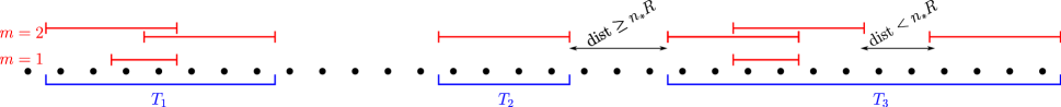
Figure 4: An example of resonant intervals $S^{(m)}_{i}$ for $m=1,2$. Here, we have chosen $R=2$ and $n_{*}=2$. The resulting collection of intervals $T_{\alpha}$ is shown.

The final resonant set is then defined as the union of $T_{\alpha}$;

$${\mathfrak{R}}=\bigcup_{\alpha}T_{\alpha}.$$

For any $T_{\alpha}$, we define

$${\mathcal{E}}_{\alpha}=\sum_{i\in T_{\alpha}}\left(h_{i}Z_{i}+\sum_{m=1}^{n_{*}}J^{m}W_{i}^{(m){\mathfrak{R}}}\right)+\sum_{m=1}^{n_{*}}\sum_{i:S_{i}^{(m)}\cap T_{\alpha}\neq\emptyset}J^{m}D_{i}^{(m)}.$$ (7.2)

The term between brackets is supported on $T_{\alpha}$. Indeed, terms $W_{i}^{(m){\mathfrak{R}}}$ with $i$ closer than distance $Rm$ to the maximum of $T_{\alpha}$ are zero, else the interval $T_{\alpha}$ would have extended further right. However, the terms $D_{i}^{(m)}$ extend beyond $T_{\alpha}$. Therefore, we define fattened intervals

$$\tilde{T}_{\alpha}=[\min(T_{\alpha})-n_{*}R+1,\max(T_{\alpha})+n_{*}R-1],$$

such that ${\mathcal{E}}_{\alpha}$ is indeed supported on $\widetilde{T}_{\alpha}$, see Figure 5.

Figure 5: We illustrate the fattened intervals $\widetilde{T}_{\alpha}$ starting from the example of Figure 4.

We note that $H^{\prime}$ can now be written as

$$H^{\prime}=\sum_{i:i\not\in{\mathfrak{R}}}h_{i}Z_{i}+\sum_{m=1}^{n_{*}}\sum_{i:S_{i}^{(m)}\cap{\mathfrak{R}}=\emptyset}J^{m}D^{(m)}_{i}+\sum_{\alpha}{\mathcal{E}}_{\alpha}+\delta H^{(n_{*})}.$$ (7.3)

The nice property of the operators ${\mathcal{E}}_{\alpha}$ is that they mutually commute for different $\alpha$, and they commute with all $Z_{i},i\not\in{\mathfrak{R}}$. In particular, for given $\alpha$, the operators ${\mathcal{E}}_{\alpha}$ and $Z_{i},i\in\widetilde{T}_{\alpha}\setminus T_{\alpha}$ form a mutually commuting family, supported on $\widetilde{T}_{\alpha}$. These operators can hence be diagonalized together in $Z$-basis. We can then construct $|T_{\alpha}|$ spin operators (in the sense of Theorem 3.1) $\tau^{\prime}_{\alpha,j},j=1,\ldots,|T_{\alpha}|$ such that $\tau^{\prime}_{j}$ are supported on $\widetilde{T}_{\alpha}$ and such that they commute with each other and with $Z_{i},i\in\widetilde{T}_{\alpha}\setminus T_{\alpha}$. The labelling by $j$ is arbitrary. We now set

$$\tau^{\prime}_{i}=\begin{cases}\tau^{\prime}_{\alpha,j}&i=\min(T_{\alpha})+j-1\\ Z_{i}&i\not\in{\mathfrak{R}}\end{cases}.$$ (7.4)

In this way we obtain a full set of $N$ spin operators $\tau^{\prime}_{i}$ that mutually commute.

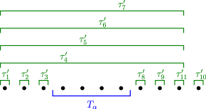
Figure 6: The support of quasi-LIOMs $\tau^{\prime}_{i}$. We have chosen $R=2$ and $n_{*}=2$.

7.3 Bounds involving quasi-LIOMs

Finally, we are ready to define the $\tau_{i}$ spin-operators as

$$\tau_{i}=e^{-\mathrm{ad}_{A}}(\tau_{i}^{\prime})$$

and to check some of the assertions of Theorem 3.1. Items 1,2,5 of Theorem 3.1 follow immediately from the corresponding properties of the $\tau_{i}^{\prime}$. For $i\not\in{\mathfrak{R}}$, we set $M_{i}=\{i\}$ and for $i\in{\mathfrak{R}}$, we set of course $M_{i}=\widetilde{T}_{\alpha}$ for the corresponding $\alpha$. Then, Item 3 follows from the locality-preserving property of $e^{-\mathrm{ad}_{A}}$, i.e. Lemma 7.2 and the fact that $||\tau_{i}^{\prime}||=1$. To get item 4, we bound, for $i\not\in{\mathfrak{R}}$;

$$||[\delta H^{(n_{*})},\tau^{\prime}_{i}]||\leq C(n_{*}+1)Re^{-\frac{1-\beta}{2}(\log(1/J))^{2-\epsilon}}.$$ (7.5)

Indeed, if we consider only the leading contributions to $\delta H^{(n_{*})}_{i}$, with support in intervals of length $(n_{*}+1)R$, then there are $(n_{*}+1)R$ sites $i$ such that $\delta H^{(n_{*})}_{i}$ contributes to the commutator, hence the factor $(n_{*}+1)R$ in the bound. One easily checks that the subleading terms in $\delta H^{(n_{*})}_{i}$ give a smaller contribution to the commutator, provided $J$ is sufficiently small, and they can be accounted for by the constant $C$ in front. For $i\in{\mathfrak{R}}$, we use analogous reasoning to derive the bound

$$||[\delta H^{(n_{*})},\tau^{\prime}_{i}]||\leq C(|\widetilde{T}_{\alpha}|+2(n_{*}+1)R)e^{-\frac{1-\beta}{2}(\log(1/J))^{2-\epsilon}}.$$

Taking $J$ small enough and recalling that $|M_{i}|=|\widetilde{T}_{\alpha}|\geq 2n_{*}R$, we obtain now item 4. of the theorem. Note that we changed $\frac{1-\beta}{2}$ to $\frac{1-\beta}{4}$ to absorb polynomial factors in $\log(1/J)$.

Figure 7: The exponential quasilocalty of quasi-LIOMs $\tau_{i}$. The spatial extend of rectangles illustrates the range of local terms, while their opaqueness illustrates their strength. The figure depicts the first $5$ strongest terms from the expansion of $\tau_{6}$ and $\tau_{18}$. Note, that $\tau_{18}$ corresponds to $\widetilde{T}_{\alpha}$ with length $|\widetilde{T}_{\alpha}|=10$, hence all quasi-LIOMs $\tau_{i}$ for $i\in[18,27]$ look the same in the above representation.

7.4 Probabilistic estimates

In Section 4, we already computed the probability of a given bond $(i,i+1)$ being resonant at the first scale for $R=2$. For higher scales and general $R$, we stated the non-resonance condition (5.8). The probability of (5.8) being violated is estimated as

$$\mathrm{Prob}(\,\min_{\eta\neq 0}\,|\sum_{i\in S_{i}^{(m)}}\eta_{i}h_{i}|<\delta)\leq\sum_{\eta\neq 0}\mathrm{Prob}(\,|\sum_{i\in S_{i}^{(m)}}\eta_{i}h_{i}\,|<\delta)\leq 3^{mR}\delta,$$ (7.6)

where the prefactor $3^{mR}$ accounts for the number of choices of $\eta$. For a single $\eta$, we choose an index $j$ such that $\eta_{j}\neq 0$ and we write $|\sum_{i}\eta_{i}h_{i}|=|h_{j}+a|$ with $a$ independent of $h_{j}$. The probability that this expression is smaller than $\delta$ is then obviously bounded by $\delta$, giving the above estimate.

Therefore, the probability to have a resonant interval of length $mR$ starting at site $i$ is bounded by

$$3^{Rm}\delta,$$

and the probability of having a resonant interval - of arbitrary length - starting at $i$ is obtained by summing this from $m=1$ to $m=n_{*}$. If a site $i$ is in the resonant set ${\mathfrak{R}}$, a resonant interval must have started somewhere in the interval $[i-2n_{*}R+1,i]$. This leads to the estimate

$$\mathrm{Prob}(i\in{\mathfrak{R}})\leq 2n_{*}R\sum_{m=1}^{n_{*}}3^{Rm}\delta\leq 4n_{*}R3^{Rn_{*}}\delta\leq J^{\beta/2},$$ (7.7)

where the last bound follows by the choice (3.1) for $n_{*}$, for $J$ small enough. The starting of a resonant interval at a site in $[i-2n_{*}R+1,i]$ is a necessary condition, but not a sufficient condition, for the event $i\in{\mathfrak{R}}$ to be true. To determine whether $i\in{\mathfrak{R}}$, we need information about resonant intervals starting in $[i-2n_{*}R+1,i+n_{*}R-1]$. This means we need information on the random variables $h_{j}$ for $j\in[i-2n_{*}R+1,i+2n_{*}R-1]$. We have now hence proven item 6. of Theorem 3.1. The first claim of item 7. is a direct consequence of the way the fattened intervals $\widetilde{T}_{\alpha}$ were defined. The bound in item 7. can be deduced in an elementary way: In order for $|M_{i}|=|\widetilde{T}_{\alpha}|\geq\ell$, we need that at least $\ell/(4n_{*}R)$ sites, spaced by $4n_{*}R$, are in ${\mathfrak{R}}$. Since these are independent events, the probability of an interval $|\widetilde{T}_{\alpha}|\geq\ell$ starting at a given site is bounded by (using item 6)

$$J^{(\beta/2)(\ell/(4n_{*}R))}\leq e^{-\frac{\beta}{8R}\log(1/J)^{\epsilon}\ell}.$$

However, for $|M_{i}|\geq\ell$, this interval can start at any site in $[i-\ell+1,i+\ell-1]$, so we multiply the above probability by $2\ell$. By readjusting constants, we then get item 7.

It is interesting to note that the requirement that $\mathrm{Prob}(i\in{\mathfrak{R}})\leq J^{\beta/2}$ forces us to let $n_{*}$ grow not faster then logarithmically in $J$. This is the reason that, as things stand, it does not make much sense to improve the combinatorial estimates in Section 6.

7.5 Proof of Theorem 3.2

For any site $i$, we define the random variable

$$Q(i)=\sum_{\alpha}|\widetilde{T}_{\alpha}|e^{-\frac{1-\beta}{2}\log(1/J)\mathrm{dist}(i,\widetilde{T}_{\alpha})}$$

that will play a major role in what follows. Let $x$ be the site at smallest distance to the site $i_{*}$, such that

$$Q(x)\leq e^{-\frac{1-\beta}{2}\log(1/J)}.$$ (7.8)

Then

Lemma 7.3.

For $J$ sufficiently small,

$$\mathrm{Prob}(\mathrm{dist}(x,i_{*})\geq\ell)\leq e^{-c_{0}(\log(1/J))^{\epsilon}\ell},\qquad c_{0}=10^{-3}\beta/R.$$

Note in particular, that there is no $\alpha$ such that $x\in\widetilde{T}_{\alpha}$. Else, $\mathrm{dist}(x,\widetilde{T}_{\alpha})=0$ and the requirement (7.8) would not be satisfied. The proof of Lemma 7.3 rests entirely on the sparsity of the resonant set ${\mathfrak{R}}$. Since it does not add any further insight, we postpone it to the Appendix.

Let us now come to Theorem 3.2. In the setup, we defined a splitting $H=H_{L}+H_{R}$ based on a fiducial point $i_{*}$. It is advantageous now to vary the fiducial point. We write therefore $H=H_{L,i}+H_{R,i}$ for any point $i$, with $H_{L,i}=\sum_{j\leq i}(h_{j}Z_{j}+JV_{j})$, cf. the expression in (3.3). In particular, we will choose the random site $x$, defined above, as the fiducial point.

We start from the expression for $H^{\prime}$ given in (7.3) and we define a left-right splitting (relative to the site $x$) of this Hamiltonian as

$$H_{L,x}^{\prime}=\sum_{\begin{subarray}{c}i:i\leq x\\ i\not\in{\mathfrak{R}}\end{subarray}}h_{i}Z_{i}+\sum_{m=1}^{n_{*}}\sum_{\begin{subarray}{c}i:i\leq x\\ S_{i}^{(m)}\cap{\mathfrak{R}}=\emptyset\end{subarray}}J^{m}D^{(m)}_{i}+\sum_{\alpha:\min\widetilde{T}_{\alpha}\leq x}{\mathcal{E}}_{\alpha}+\sum_{i:i\leq x}\delta H^{(n_{*})}_{i}$$ (7.9)

and $H_{R,x}^{\prime}=H^{\prime}-H_{L,x}^{\prime}$. Now we split

$$e^{\mathrm{ad}_{A}}[H_{L,x},H]=[e^{\mathrm{ad}_{A}}(H_{L,x})-H_{L,x}^{\prime},H^{\prime}]+[H_{L,x}^{\prime},H^{\prime}].$$ (7.10)

Let us start by estimating the commutator $[H_{L,x}^{\prime},H^{\prime}]$ on the right-hand side.

Lemma 7.4.

For sufficiently small $J$,

$$||[H_{L,x}^{\prime},H^{\prime}]||\leq e^{-\frac{1-\beta}{4}(\log(1/J))^{2-\epsilon}}.$$

Proof.

We write $K_{j}$ to denote local terms of the type $h_{j}Z_{j},J^{m}D_{i}^{(m)}$ in the expression (7.3), so that this expression consists of the contributions

1. $\mathop{\sum}\limits_{j\leq x,i>x}[K_{j},\delta H^{(n_{*})}_{i}]$.

2. $\mathop{\sum}\limits_{j\leq x,i>x}[\delta H^{(n_{*})}_{j},K_{i}]$.

3. $\mathop{\sum}\limits_{j\leq x,i>x}[\delta H^{(n_{*})}_{j},\delta H^{(n_{*})}_{i}]$.

Then there are also the contributions involving ${\mathcal{E}}_{\alpha}$, they are of the form

1. $\mathop{\sum}\limits_{\begin{subarray}{c}i>x\\ \alpha:\min\widetilde{T}_{\alpha}\leq x\end{subarray}}[{\mathcal{E}}_{\alpha},\delta H^{(n_{*})}_{i}].$

2. $\mathop{\sum}\limits_{\begin{subarray}{c}i\leq x\\ \alpha:\min\widetilde{T}_{\alpha}>x\end{subarray}}[\delta H^{(n_{*})}_{i},{\mathcal{E}}_{\alpha}]$.

The contributions 1.,2.,3. together are bounded by

$$C((n_{*}+1)R)^{2}e^{-\frac{1-\beta}{2}(\log(1/J))^{2-\epsilon}},$$

where we used the same reasoning as for the bound (7.5). Similarly, contributions 4.,5. are bounded together by

$$CQ(x)((n_{*}+1)R)e^{-\frac{1-\beta}{2}(\log(1/J))^{2-\epsilon}},$$

where $Q(x)$ is the random variable defined above Lemma 7.3. To get this estimate, we use that $||{\mathcal{E}}_{\alpha}||\leq C|\widetilde{T}_{\alpha}|$ and that there is no interval $\widetilde{T}_{\alpha}$ containing $x$, see the remark following Lemma 7.3. ∎

We now move to the first term on the right-hand side of (7.10).

Lemma 7.5.

There is an observable $O^{\prime}$ with

$$||O^{\prime}||\leq CJ^{\frac{1-\beta}{4R}}$$

satisfying

$$[e^{\mathrm{ad}_{A}}(H_{L,x})-H_{L,x}^{\prime},H^{\prime}]=[O^{\prime},H^{\prime}].$$

Proof.

Let $\tr_{>x}$ be the normalized partial trace over the region $\{i\,|\,i>x\}$. Then we have, since $e^{\mathrm{ad}_{A}}(H)=H^{\prime}$,

$$0=\tr_{>x}[e^{\mathrm{ad}_{A}}(H)]-\tr_{>x}[H^{\prime}].$$ (7.11)

By a standard application of Lieb-Robinson bounds (see the discussion following Lemma 7.2), we have

$$||e^{\mathrm{ad}_{A}}(H_{L,x})-\tr_{>x}[e^{\mathrm{ad}_{A}}(H_{L,x})]||\leq CJ^{\frac{1-\beta}{4R}},$$ (7.12)

for $J$ small enough. By similar reasoning, we get

$$||\tr[e^{\mathrm{ad}_{A}}(H_{R,x})]-\tr_{>x}[e^{\mathrm{ad}_{A}}(H_{R,x})]||\leq CJ^{\frac{1-\beta}{4R}},$$ (7.13)

where $\tr[\cdot]$ is the normalized trace over the whole chain. We can also estimate

$$\tr_{>x}[H^{\prime}]-H_{L,x}^{\prime}=\tr[H^{\prime}_{R,x}]+\sum_{l}(\tr_{>x}[A_{l}]-A_{l}),$$ (7.14)

where the sum over $A_{l}$ runs over all local terms included in the definition of $H^{\prime}_{L}$, in (7.9), but with support extending to the right of $x$. By the remark following Lemma 7.3, none of these local terms is of the form ${\mathcal{E}}_{\alpha}$, and so they are all of the form $J^{m}D^{(m)}_{i}$. Therefore, by Lemma 7.1, we have good bounds on all the $A_{l}$ and we can estimate

$$\sum_{l}||\tr_{>x}[A_{l}]-A_{l}||\leq 2\sum_{l}||A_{l}||\leq CJ^{\frac{1-\beta}{2}}.$$ (7.15)

Starting from (7.11) and using (7.12, 7.13, 7.14 and 7.15) we get

$$||e^{\mathrm{ad}_{A}}(H_{L,x})-H_{L,x}^{\prime}+a||\leq CJ^{\frac{1-\beta}{4R}},\qquad a=\tr[e^{\mathrm{ad}_{A}}(H_{R,x})]-\tr[H_{R,x}^{\prime}].$$

Setting $O^{\prime}=e^{\mathrm{ad}_{A}}(H_{L,x})-H_{L,x}^{\prime}+a$ and using that $a$ is a number, i.e. it commutes with all operators, we get the claim of the lemma. ∎

We turn now to the proof of Theorem 3.2. Let us apply $e^{-\mathrm{ad}_{A}}$ to (7.10) and use Lemma 7.5 and Lemma 7.4 obtaining

$$||[H_{L,x},H]-[e^{-\mathrm{ad}_{A}}(O^{\prime}),H]||\leq e^{-\frac{1-\beta}{4}(\log(1/J))^{2-\epsilon}}$$ (7.16)

To get Theorem 3.2, we have to go back to the fiducial site $i_{*}$, To that order, we remark that

$$H_{L,i_{*}}-H_{L,x}=O^{\prime\prime},\qquad||O^{\prime\prime}||\leq\mathrm{dist}(x,i_{*})(1+J).$$

Setting now

$$O=O^{\prime\prime}+e^{-\mathrm{ad}_{A}}(O^{\prime})$$

we obtain the claim of Theorem 3.2.

Appendix

In this appendix, we prove of Lemma 7.3. Let us abbreviate

$$\kappa=\frac{1-\beta}{2}\log(\frac{1}{J}),\qquad\nu=\frac{\beta}{8R}\left(\log(\frac{1}{J})\right)^{\epsilon},$$

so that we can rewrite

$$Q(i)=\sum_{\alpha}|\widetilde{T}_{\alpha}|e^{-\kappa\mathrm{dist}(i,\widetilde{T}_{\alpha})}.$$

We need the following auxiliary result

Lemma 7.6.

If $Q(i)>M$ for some site $i$ and $M>0$, then there exists $\alpha$ such that

$$|\widetilde{T}_{\alpha}|e^{-\kappa\mathrm{dist}(i,\widetilde{T}_{\alpha})/2}\geq\frac{M}{2}(1-e^{-\kappa/2}).$$ (7.17)

Proof.

If there were no such $\alpha$, we dominate

$$Q(i)<\frac{M}{2}(1-e^{-\kappa/2})\sum_{\alpha}e^{-\kappa\mathrm{dist}(i,\widetilde{T}_{\alpha})/2}\leq M(1-e^{-\kappa/2})\sum_{j=0}^{\infty}e^{-\kappa j/2}\leq(1-e^{-\kappa/2})\frac{M}{1-e^{-\kappa/2}}.$$

∎

We use Lemma 7.6 with $M=e^{-\kappa}$. If site $i$ satisfies the inequality (7.17) for some $\alpha$, then, for $\kappa$ large enough (hence $J$ small enough),

$$\mathrm{dist}(i,\widetilde{T}_{\alpha}) \leq\frac{2}{\kappa}\log|\widetilde{T}_{\alpha}|-\frac{2}{\kappa}\log(\frac{e^{-\kappa}}{2}(1-e^{-\kappa/2}))$$

$$\leq\frac{2}{\kappa}\log|\widetilde{T}_{\alpha}|+3\leq 4|\widetilde{T}_{\alpha}|.$$ (7.18)

We recall that Lemma 7.3 depends on a fiducial site $i_{*}$ and we define intervals centered on $i_{*}$:

$$B_{L}=\{j:\mathrm{dist}(i_{*},j)\leq L/2\}.$$

We will prove below that

$$\mathrm{Prob}(\forall i\in B_{2\ell}:Q(i)\geq e^{-\kappa})\leq e^{-\frac{1}{72}\nu\ell},\qquad\text{for}\,\ell>16n_{*}R.$$ (7.19)

For $\ell\leq 16n_{*}R$, the same bound follows by similar but simpler considerations as those presented below. In particular, in Case 2 below, it suffices to exhibit a single site in ${\mathfrak{R}}\cap B_{2\ell}$ and use the bound from Theorem 3.1 item 6). Once (7.19) is proven for all $\ell$, Lemma 6.2 follows directly.

Let $E_{L}$ be the event that there is an interval $K$ of length $L$ such that $K\subset{\mathfrak{R}}$ and $\mathrm{dist}(K,i_{*})\leq 14L$. Then

$$\mathrm{Prob}(E_{L})\leq 29Le^{-\nu L}$$

by the discussion in subsection 7.4. We now prove (7.19) by distinguishing two cases, assuming that the event in (7.19) holds.

Case 1: The event $E_{L}$ holds for some $L>\ell/16$. The probability of this is bounded by $29(\ell/16+1)e^{-\nu(\ell/16-1)}\leq e^{-\frac{1}{72}\nu\ell}$, and so in this case (7.19) is proven.

Case 2: The event $E_{L}$ does not hold for any $L\geq\ell/16$. Consider a site $j\in B_{\ell/8}$. Since it satisfies $Q(j)>e^{-\kappa}$, there must be at least one $\alpha$ such that $\mathrm{dist}(j,\widetilde{T}_{\alpha})\leq 4|\widetilde{T}_{\alpha}|$, by (7.18), and hence $\mathrm{dist}(i_{*},T_{\alpha})\leq 4|\widetilde{T}_{\alpha}|+n_{*}R+\ell/16$. Since $E_{L}$ does not hold for any $L\geq\ell/16$ (by assumption), any such $\alpha$ satisfies $\widetilde{T}_{\alpha}\subset B_{2\ell}$ as $|\widetilde{T}_{\alpha}|<|T_{\alpha}|+2n_{*}R$ and $\ell>16n_{*}R$. For any such $\widetilde{T}_{\alpha}$ there exist at most $9|\widetilde{T}_{\alpha}|$ sites satisfying the equation (7.18). On the other hand this equation has to be satisfied for all sites in $B_{\ell/8}$. Therefore, we conclude

$$\sum_{\alpha:\widetilde{T}_{\alpha}\subset B_{2\ell}}9|\widetilde{T}_{\alpha}|\geq|B_{\ell/8}|.$$

This leads to the lower bound

$$|{\mathfrak{R}}\cap B_{2\ell}|\geq\frac{\ell}{72}.$$

By the discussion in subsection 7.4, this means that there are least $\frac{\ell/72}{4n_{*}R}$ sites in ${\mathfrak{R}}$, sufficiently spaced so as to be independent. We conclude that the probability of this occurring is bounded by $e^{-\frac{1}{72}\nu\ell}$.

References

• [1] D. M. Basko, I. L. Aleiner, and B. L. Altshuler, “Metal-insulator transition in a weakly interacting many-electron system with localized single-particle states,” Ann. Phys. (Amsterdam), vol. 321, pp. 1126–1205, 2006.
• [2] I. V. Gornyi, A. D. Mirlin, and D. G. Polyakov, “Interacting electrons in disordered wires: Anderson localization and low-t transport,” Physical review letters, vol. 95, no. 20, p. 206603, 2005.
• [3] M. Žnidarič, T. Prosen, and P. Prelovšek, “Many-body localization in the heisenberg x x z magnet in a random field,” Physical Review B, vol. 77, no. 6, p. 064426, 2008.
• [4] V. Oganesyan and D. A. Huse, “Localization of interacting fermions at high temperature,” Physical review b, vol. 75, no. 15, p. 155111, 2007.
• [5] A. Pal and D. A. Huse, “Many-body localization phase transition,” Physical review b, vol. 82, no. 17, p. 174411, 2010.
• [6] V. Ros, M. Müller, and A. Scardicchio, “Integrals of motion in the many-body localized phase,” Nuclear Physics B, vol. 891, pp. 420–465, 2015.
• [7] J. A. Kjäll, J. H. Bardarson, and F. Pollmann, “Many-body localization in a disordered quantum ising chain,” Physical review letters, vol. 113, no. 10, p. 107204, 2014.
• [8] D. A. Huse, R. Nandkishore, and V. Oganesyan, “Phenomenology of fully many-body-localized systems,” Phys. Rev. B, vol. 90, p. 174202, 2014.
• [9] D. J. Luitz, N. Laflorencie, and F. Alet, “Many-body localization edge in the random-field Heisenberg chain,” Physical Review B, vol. 91, no. 8, p. 081103, 2015.
• [10] J. Z. Imbrie, “Multi-scale Jacobi method for Anderson localization,” Commun. Math. Phys., vol. 341, pp. 491–521, 2016.
• [11] M. Schreiber, S. S. Hodgman, P. Bordia, H. P. Lüschen, M. H. Fischer, R. Vosk, E. Altman, U. Schneider, and I. Bloch, “Observation of many-body localization of interacting fermions in a quasi-random optical lattice,” Science, vol. 349, no. 6250, pp. 842–845, 2015.
• [12] D. A. Abanin, E. Altman, I. Bloch, and M. Serbyn, “Colloquium: Many-body localization, thermalization, and entanglement,” Rev. Mod. Phys., vol. 91, p. 021001, May 2019.
• [13] R. Nandkishore and D. A. Huse, “Many-body localization and thermalization in quantum statistical mechanics,” Annual Review of Condensed Matter Physics, vol. 6, no. 1, pp. 15–38, 2015.
• [14] V. Oganesyan, A. Pal, and D. A. Huse, “Energy transport in disordered classical spin chains,” Phys. Rev. B, vol. 80, p. 115104, Sep 2009.
• [15] D. M. Basko, “Weak chaos in the disordered nonlinear Schrödinger chain: destruction of Anderson localization by Arnold diffusion,” Annals of Physics, vol. 326, no. 7, pp. 1577–1655, 2011.
• [16] F. Huveneers, “Drastic fall-off of the thermal conductivity for disordered lattices in the limit of weak anharmonic interactions,” Nonlinearity, vol. 26, pp. 837–854, feb 2013.
• [17] W. De Roeck and F. Huveneers, “Asymptotic localization of energy in nondisordered oscillator chains,” Communications on Pure and Applied Mathematics, vol. 68, no. 9, pp. 1532–1568, 2015.
• [18] W. De Roeck and F. Huveneers, “Asymptotic quantum many-body localization from thermal disorder,” Commun. Math. Phys., vol. 332, pp. 1017–1082, 2014.
• [19] J. Fröhlich, T. Spencer, and C. E. Wayne, “Localization in disordered, nonlinear dynamical systems,” Journal of statistical physics, vol. 42, pp. 247–274, 1986.
• [20] G. Benettin, J. Fröhlich, and A. Giorgilli, “A Nekhoroshev-type theorem for Hamiltonian systems with infinitely many degrees of freedom,” Communications in mathematical physics, vol. 119, pp. 95–108, 1988.
• [21] J. Pöschel, “Small divisors with spatial structure in infinite dimensional hamiltonian systems,” Communications in mathematical physics, vol. 127, no. 2, pp. 351–393, 1990.
• [22] M. Johansson, G. Kopidakis, and S. Aubry, “KAM tori in 1D random discrete nonlinear Schrödinger model?,” Europhysics Letters, vol. 91, no. 5, p. 50001, 2010.
• [23] W.-M. Wang and Z. Zhang, “Long time Anderson localization for the nonlinear random Schrödinger equation,” Journal of Statistical Physics, vol. 134, pp. 953–968, 2009.
• [24] S. Fishman, Y. Krivolapov, and A. Soffer, “Perturbation theory for the nonlinear Schrödinger equation with a random potential,” Nonlinearity, vol. 22, no. 12, p. 2861, 2009.
• [25] S. Fishman, Y. Krivolapov, and A. Soffer, “The nonlinear Schrödinger equation with a random potential: results and puzzles,” Nonlinearity, vol. 25, no. 4, p. R53, 2012.
• [26] W. De Roeck and F. Huveneers, “Stability and instability towards delocalization in many-body localization systems,” Physical Review B, vol. 95, no. 15, p. 155129, 2017.
• [27] D. J. Luitz, F. Huveneers, and W. De Roeck, “How a small quantum bath can thermalize long localized chains,” Physical review letters, vol. 119, no. 15, p. 150602, 2017.
• [28] J. Šuntajs, J. Bonča, T. Prosen, and L. Vidmar, “Quantum chaos challenges many-body localization,” Physical Review E, vol. 102, no. 6, p. 062144, 2020.
• [29] D. Sels, “Bath-induced delocalization in interacting disordered spin chains,” Physical Review B, vol. 106, no. 2, p. L020202, 2022.
• [30] A. Morningstar, L. Colmenarez, V. Khemani, D. J. Luitz, and D. A. Huse, “Avalanches and many-body resonances in many-body localized systems,” Physical Review B, vol. 105, no. 17, p. 174205, 2022.
• [31] T. Kuwahara, T. Mori, and K. Saito, “Floquet–Magnus theory and generic transient dynamics in periodically driven many-body quantum systems,” Annals of Physics, vol. 367, pp. 96 – 124, 2016.
• [32] N. H. Lindner, E. Berg, and M. S. Rudner, “Universal chiral quasisteady states in periodically driven many-body systems,” Phys. Rev. X, vol. 7, p. 011018, Feb 2017.
• [33] T. Gulden, E. Berg, M. S. Rudner, and N. Lindner, “Exponentially long lifetime of universal quasi-steady states in topological Floquet pumps,” SciPost Physics, vol. 9, Jul 2020.
• [34] T. Mori, T. Kuwahara, and K. Saito, “Rigorous bound on energy absorption and generic relaxation in periodically driven quantum systems,” Physical review letters, vol. 116, no. 12, p. 120401, 2016.
• [35] D. Abanin, W. De Roeck, W. W. Ho, and F. Huveneers, “A rigorous theory of many-body prethermalization for periodically driven and closed quantum systems,” Communications in Mathematical Physics, vol. 354, no. 3, pp. 809–827, 2017.
• [36] D. V. Else, P. Fendley, J. Kemp, and C. Nayak, “Prethermal strong zero modes and topological qubits,” Physical Review X, vol. 7, no. 4, p. 041062, 2017.
• [37] D. V. Else, B. Bauer, and C. Nayak, “Prethermal phases of matter protected by time-translation symmetry,” Physical Review X, vol. 7, no. 1, p. 011026, 2017.
• [38] P. T. Dumitrescu, R. Vasseur, and A. C. Potter, “Logarithmically slow relaxation in quasiperiodically driven random spin chains,” Physical review letters, vol. 120, no. 7, p. 070602, 2018.
• [39] F. Huveneers and J. Lukkarinen, “Prethermalization in a classical phonon field: Slow relaxation of the number of phonons,” Physical review research, vol. 2, no. 2, p. 022034, 2020.
• [40] D. V. Else, W. W. Ho, and P. T. Dumitrescu, “Long-lived interacting phases of matter protected by multiple time-translation symmetries in quasiperiodically driven systems,” Physical Review X, vol. 10, no. 2, p. 021032, 2020.
• [41] P. Anderson, “Absence of diffusion in certain random lattices,” Phys. Rev., vol. 109, pp. 1492–1505, 1958.
• [42] H. Kunz and B. Souillard, “Sur le spectre des opérateurs aux différences finies aléatoires,” Communications in Mathematical Physics, vol. 78, pp. 201–246, 1980.
• [43] J. Fröhlich and T. Spencer, “Absence of diffusion in the Anderson tight binding model for large disorder or low energy,” Commun. Math. Phys., vol. 88, pp. 151–184, 1983.
• [44] M. Aizenman and S. Warzel, Random operators, vol. 168. American Mathematical Soc., 2015.
• [45] M. B. Hastings, “Locality in quantum systems,” Quantum Theory from Small to Large Scales, vol. 95, pp. 171–212, 2010.
• [46] B. Nachtergaele, R. Sims, and A. Young, “Quasi-locality bounds for quantum lattice systems. I. Lieb-Robinson bounds, quasi-local maps, and spectral flow automorphisms,” Journal of Mathematical Physics, vol. 60, no. 6, p. 061101, 2019.
• [47] J. Berges, S. Borsányi, and C. Wetterich, “Prethermalization,” Phys. Rev. Lett., vol. 93, p. 142002, Sep 2004.
• [48] M. Eckstein, M. Kollar, and P. Werner, “Thermalization after an interaction quench in the Hubbard model,” Physical review letters, vol. 103, no. 5, p. 056403, 2009.
• [49] K. Mallayya, M. Rigol, and W. De Roeck, “Prethermalization and thermalization in isolated quantum systems,” Phys. Rev. X, vol. 9, p. 021027, May 2019.
• [50] B. Bertini, F. H. Essler, S. Groha, and N. J. Robinson, “Prethermalization and thermalization in models with weak integrability breaking,” Physical review letters, vol. 115, no. 18, p. 180601, 2015.
• [51] A. Bastianello, A. De Luca, and R. Vasseur, “Hydrodynamics of weak integrability breaking,” Journal of Statistical Mechanics: Theory and Experiment, vol. 2021, no. 11, p. 114003, 2021.
• [52] D. A. Abanin, W. De Roeck, W. W. Ho, and F. Huveneers, “Effective Hamiltonians, prethermalization, and slow energy absorption in periodically driven many-body systems,” Physical Review B, vol. 95, no. 1, p. 014112, 2017.
• [53] I. Schur, “Bemerkungen zur Theorie der beschränkten Bilinearformen mit unendlich vielen Veränderlichen,” Journal für die reine und angewandte Mathematik, pp. 1–28, 1911.
• [54] R. A. Horn and R. Mathias, “Block-matrix generalizations of Schur’s basic theorems on Hadamard products,” Linear Algebra and its Applications, vol. 172, pp. 337–346, 1992.
• [55] S. Bravyi, M. B. Hastings, and F. Verstraete, “Lieb-Robinson bounds and the generation of correlations and topological quantum order,” Physical review letters, vol. 97, no. 5, p. 050401, 2006.