Learning to Distill Global Representation for Sparse-View CT

Abstract

Sparse-view computed tomography (CT)—using a small number of projections for tomographic reconstruction—enables much lower radiation dose to patients and accelerated data acquisition. The reconstructed images, however, suffer from strong artifacts, greatly limiting their diagnostic value. Current trends for sparse-view CT turn to the raw data for better information recovery. The resultant dual-domain methods, nonetheless, suffer from secondary artifacts, especially in ultra-sparse view scenarios, and their generalization to other scanners/protocols is greatly limited. A crucial question arises: have the image post-processing methods reached the limit? Our answer is not yet. In this paper, we stick to image post-processing methods due to great flexibility and propose global representation(GloRe) distillation framework for sparse-view CT, termed GloReDi. First, we propose to learn GloRe with Fourier convolution, so each element in GloRe has an image-wide receptive field. Second, unlike methods that only use the full-view images for supervision, we propose to distill GloRe from intermediate-view reconstructed images that are readily available but not explored in previous literature. The success of GloRe distillation is attributed to two key components: representation directional distillation to align the GloRe directions, and band-pass-specific contrastive distillation to gain clinically important details. Extensive experiments demonstrate the superiority of the proposed GloReDi over the state-of-the-art methods, including dual-domain ones. The source code is available at https://github.com/longzilicart/GloReDi.

1 Introduction

X-ray CT is one of the major modalities widely used in clinical screening and diagnosis. Despite the benefits, there have been growing concerns that X-ray radiation exposure could increase the risk of cancer induction [48]. Following the As Low As Reasonably Achievable (ALARA) principle in the medical community [36], efforts have been made to lower the radiation dose while maintaining imaging quality [20]. Sparse-view CT is one of the effective solutions which reduces the radiation by sampling part of the projection data, a.k.a sinogram, for image reconstruction, as shown in Fig. 1. However, analytical reconstruction algorithms such as filtered back projection (FBP) produce inferior image quality with globally severe streak artifacts, significantly compromising its diagnosis value. How to effectively reconstruct the sparse-view CT remains challenging and, hence, is gaining increasing attention in the computer vision and medical imaging communities.

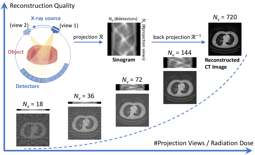
Figure 1: Sparse-view CT only uses a few projection views for tomographic reconstruction, thus providing fast and low-dose CT scanning. However, the reconstruction results of the conventional method suffer from severe global streak artifacts.

Image-domain methods regard sparse-view CT reconstruction as an image post-processing task on the FBP-reconstructed images and have achieved exciting performance on streaking artifacts removal and structure preservation [5, 22, 59, 32]. However, due to the limited receptive field, these methods have difficulty in modeling the global information efficiently, thus leading to suboptimal results. Current dominant methods turn to the help of sinogram by restoring the sinogram and performing CT image post-processing simultaneously [31, 17, 47, 29]. Specifically, in addition to the image domain methods, deep neural networks are also applied to interpolate the missing data in sinogram so that the reconstructed images can be recovered in a global manner [25, 10].

Despite the common success of dual-domain methods, they suffer from unsatisfactory and unstable performance due to the following reasons. First, the processing of sinogram data is sensitive and even subtle changes may remarkably affect the reconstructed images and introduce stubborn secondary artifacts that are hard to be eliminated. Second, in ultra sparse-view scenarios, inpainting methods are unable to accurately restore the excessive missing raw data; e.g., inpainting sparse CT data of 18 views to the full CT data of 720 views only retains about 2.5% of the valid information, in which the involvement of sinogram processing makes the learning more difficult and compromise the performance [47, 29]. Third, it is often impractical to access sinogram data given the privacy and commercial concerns, and if accessible, the requirement of raw data greatly limits the generalization to other scanners/protocols.

Motivation.

Given the great flexibility of the image domain methods, we arise a critical question in this paper: have the image domain (post-processing) methods reached the limits? Our answer is not yet, given the following observations. First, the existing image-domain methods typically suffer from limited receptive field, which fails to extract and recover the global information efficiently [44], given that streak artifacts are spread globally on the reconstructed images as shown in Fig. 1. Second, the existing image-domain methods typically use the full-view images as the unique supervision to improve the image quality in an end-to-end manner [59, 22]. They ignore the importance of representation learning, especially global representation (GloRe), making the artifact removal and detail recovery entangled, and leading to sub-optimal results due to the significant gap between sparse- and full-view. Third, the intermediate-view reconstructed images can be readily available during data preparation, but to the best of our knowledge, they are surprisingly neglected in the past literature. We argue that they can provide extra information and build bridges for sparse- and full-view CT reconstruction.

To address the abovementioned issues, we propose a novel image-domain method for sparse-view CT reconstruction. First, to address the limited receptive field inherent in conventional convolutional neural networks, we propose to learn GloRe with fast Fourier convolution (FFC) [7], so each element in GloRe has an image-wide receptive field. This global nature allows artifacts and information, spread over the entire image, to be better modeled while also easing the alignment of the representations from different views. Second, to leverage extra supervision from intermediate-view CT images, we propose a novel distillation framework to learn better GloRe, termed GloReDi, which contains a parallel teacher network to distill knowledge from the readily intermediate-view images to provide high-quality and appropriate guidance for learning the GloRe of sparse-view CT images. Specifically, we first leverage intermediate-view reconstructed images to train a teacher network, which is then used to guide the learning of the student model (i.e. the sparse-view CT). The distillation scheme benefits GloRe in two folds: (1) representation directional distillation that aligns the directions between the student and teacher GloRe, which provides appropriate supervision considering the massive information loss due to the domain gaps between CT images with different views; and (2) band-pass-specific contrastive distillation that utilizes contrastive learning solely on the band-pass components to help distill the specific clinical value of each CT image without compromising the reconstruction accuracy.

Contributions.

In summary, our contributions are listed as follows. First, we propose the global representation (GloRe) learning for sparse-view CT with Fourier convolution, which, to the best of our knowledge, is the first study to emphasize on the representation learning for image post-processing in sparse-view CT. Second, we propose a novel GloRe distillation framework, which can leverage the extra supervision from intermediate-view reconstructed images for high-quality information recovery and reconstruction. Third, we present representation directional distillation and band-pass-specific contrastive distillation for distilling GloRe to align the representation directions and gain clinically important details. Last, extensive experimental results demonstrate the superiority of GloReDi over the state-of-the-art sparse-view CT reconstruction methods in terms of quantitative metrics and visual comparison.

2 Detailed Related Work

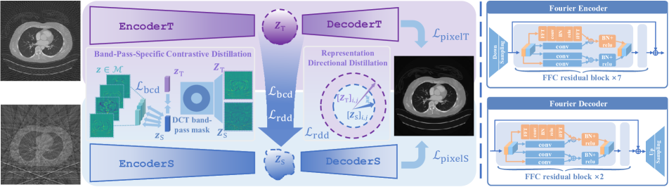
Figure 2: Overview of the proposed GloReDi for sparse-view CT reconstruction. GloReDi facilitates efficient information recovery by learning to distill the global representation from intermediate-view images.

2.1 Deep-learning-based Sparse-view CT

Numerous model-based iterative reconstruction (IR) methods have been developed to solve the sparse-view CT problem, mainly utilizing the sparsity of the total variation (TV) of the image [53, 4, 23, 37, 33, 12, 52]. However, most of them suffer from over-smoothed results, hand-crafted tuning for each image, and extremely high computation cost [47], limiting their clinical application. In contrast, deep learning methods are often faster and more accessible, thus arousing attention in this field. Among them, most image-domain methods regard sparse-view CT reconstruction as an image post-processing task. RedCNN [5], FBPConvNet [22], and DDNet [59] are proposed to reconstruct the sparse-view CT by the convolutional neural network (CNN). These methods achieve competitive performance on streak artifact removal and structure preservation compared to conventional ones, but most of them fail to capture the global context and underperform in global reconstruction and artifact removal. Since streak artifacts result directly from the incomplete projection views, various methods are proposed to remove the artifacts by interpolating sinogram data [25, 10]. Further, dual-domain methods were becoming popular for their superior reconstruction performance by combining the knowledge of both domains. DuDoNet [31] first proposed a novel Radon inversion layer linking the gradient between the image and sinogram domain networks. Furthermore, various techniques have been proposed to enhance dual domain approaches through network design [6, 1] and unrolling architecture [58]. Recently, Transformer [46] has been introduced to dual-domain methods for its capability of capturing long-range dependencies, achieving superior performance [47, 29, 50]. However, the problems of the irreversible secondary artifacts and additional computational costs are not well addressed, and the requirement of raw data greatly limits their generalizability to other CT scanners/protocols. In this work, we challenge reconstructing sparse-view CT without raw data while still achieving state-of-the-art results.

2.2 Knowledge Distillation

Knowledge distillation transfers rich knowledge from teacher models to lightweight student models in the label or feature domains, mainly applied in model compression and acceleration [15, 42]. Among various approaches, feature-based knowledge distillation is extensively applied in image restoration tasks such as image super-resolution [16, 38, 27, 14]. It minimizes the distance between feature representations to learn richer information from the teacher model compared to softened labels [49]. Further, contrastive representation distillation is proposed to exploit the structural characteristics among different samples by harnessing the discriminative representations, thereby enhancing differentiation within data [8, 19, 45]. This work distills knowledge from the intermediate-view images to enhance the sparse-view CT reconstruction.

2.3 Frequency Methods in Deep Learning

Frequency methods have been widely used in digital image processing and machine learning [2]. Wavelet convolution [32] and fast Fourier convolution [7] have been proposed to provide a larger/global receptive field, achieving great success in image restoration tasks [44]. Frequency methods have also yielded promising results in domain adaption and image translation, mainly by taking advantage of domain-invariant spectrum components [55, 18, 57, 3, 56]. Previous research also shows that particular features and details can be better extracted in the frequency domain, leading to improvements in camouflaged object detection [60], face forgery detection [21, 28], and face editing [9]. Frequency-based networks have also made notable strides in CT reconstruction. Previous studies [26, 1] employ multi-wavelet CNN [32] in both sinogram and image domain to suppress artifacts, substituting the pooling operator with wavelet transforms to achieve a larger receptive field. However, since both the Haar filter-based wavelet transform and convolution are applied on the spatial feature map, these methods struggle to capture global representation effectively. Recent research has demonstrated that employing convolution in the Fourier domain can efficiently eliminate the global artifacts [34, 30]. In this work, we utilize a frequency-based network for global representation learning, enhancing clinically critical features by band-pass-specific contrastive distillation.

3 Method

3.1 Problem Definition

Assume we have a two-dimensional (2D) CT slice of size $N\times N$, $\bm{I}\in\mathbb{R}^{N\times N}$, where each pixel contains the attenuation coefficient of the corresponding human body. The raw data or sinogram from the CT scanning, $\bm{S}\in\mathbb{R}^{N_{\mathrm{v}}\times N_{\mathrm{d}}}$, can be obtained via the Radon transform [40], where $N_{\mathrm{v}}$ and $N_{\mathrm{d}}$ denote the number of projection views and the number of the detectors, respectively. Inversely, the image reconstruction process can be expressed as $\bm{I}=\mathcal{R}^{-1}(\bm{S})$, where $\mathcal{R}^{-1}$ denotes the inverse Radon transform such as FBP. Ideally, when $N_{\mathrm{v}}$ is sufficiently large, FBP can produce pleasing image quality. However, when $N_{\mathrm{v}}$ is fairly small, the image reconstruction of so-called sparse-view CT becomes an undetermined problem.

Here, we use $\bm{I}_{\mathrm{F}}$ and $\bm{I}_{\mathrm{S}}$ to represent the reconstructed images from full view (i.e. ground-truth) and sparse view, respectively. The image-domain methods for sparse-view CT are to improve the image quality of $\bm{I}_{\mathrm{S}}$ towards $\bm{I}_{\mathrm{F}}$ through a neural network $\mathcal{F}$. That is, the output of the network, $\widehat{\bm{I}}_{\mathrm{S}}=\mathcal{F}(\bm{I}_{\mathrm{S}})$, is expected to be of comparable quality to the full-view ground-truth. In addition, we also use the images, $\bm{I}_{\mathrm{T}}$, reconstructed from an intermediate number of projection views that are between sparse and full views, as the teacher supervision, forming a student-teacher framework where the teacher encoder with $\bm{I}_{\mathrm{T}}$ supervises the training of student encoder with $\bm{I}_{\mathrm{S}}$.

3.2 Overview of Our GloReDi

Fig. 2 presents the proposed GloReDi, which mainly consists of four parts: two encoders to learn global representations (GloRe) from sparse- and intermediate-view reconstructed images, $\bm{I}_{\mathrm{S}}$, and $\bm{I}_{\mathrm{T}}$, respectively, and two decoders to produce the final processed images from GloRe. In addition to learning GloRe with Fourier convolution, we have two novel modules to perform distillation from the teacher network: (1) representation directional distillation to align the directions between the student and teacher GloRes; and (2) band-pass-specific contrastive distillation to distill the clinically important features for better detail recovery.

Next, we detail each of the proposed components.

3.3 Global Representation Learning

The key technique behind the proposed network is the global representation learning with fast Fourier convolution (FFC) [7]. Concretely, FFC first applies real Fourier transform to get the frequency feature map and then performs convolution on frequency components before finally back transforming the frequency features as shown in Fig. 2. Therefore, GloRe from sparse-view images $\bm{I}_{\mathrm{S}}$ is learned by a Fourier-based encoder network as follows:

$$\bm{Z}_{\mathrm{S}}=\texttt{encoderS}(\bm{I}_{\mathrm{S}}),$$ (1)

where $\bm{Z}_{\mathrm{S}}\in\mathbb{R}^{N_{\mathrm{w}}\times N_{\mathrm{h}}\times N_{\mathrm{c}}}$ denotes GloRe extracted from the sparse-view reconstructed image $\bm{I}_{\mathrm{S}}$ through the (student) encoder encoderS and $N_{\mathrm{w}}\times N_{\mathrm{h}}\times N_{\mathrm{c}}$ denotes the width, height, and channel size of GloRe. Compared to the vanilla convolution with a limited receptive field, FFC works in the frequency domain, so each element in GloRe contains the global information of the sparse-view images by using an image-wide receptive field, representing patterns of artifacts and the image contents simultaneously. Furthermore, such global nature can aid in modeling the artifact and information distributed throughout the image while easing the alignment between GloRe of different views.

3.4 Global Representation Distillation

In the context of sparse-view CT, images with an intermediate view $\bm{I}_{\mathrm{T}}$ can be easily obtained from the full-view sinogram as extra supervision. To get the teacher representation from $\bm{I}_{\mathrm{T}}$, a parallel teacher encoder encoderT, using the same architecture as encoderS but with different weights, takes $\bm{I}_{\mathrm{T}}$ as input and yields teacher GloRe $\bm{Z}_{\mathrm{T}}$ of the same shape with $\bm{Z}_{\mathrm{S}}$ as follows:

$$\bm{Z}_{\mathrm{T}}=\texttt{encoderT}(\bm{I}_{\mathrm{T}}).$$ (2)

$\bm{Z}_{\mathrm{T}}$ can be regarded as a high-quality pseudo target for student GloRe in the same latent space since richer information can be extracted from $\bm{I}_{\mathrm{T}}$. Exploring distillation from $\bm{I}_{\mathrm{T}}$ is obviously easier than that of $\bm{I}_{\mathrm{F}}$ given the significant gap between $\bm{I}_{\mathrm{S}}$ and $\bm{I}_{\mathrm{F}}$.

Intuitively, $\bm{Z}_{\mathrm{S}}$ should be similar to $\bm{Z}_{\mathrm{T}}$ if the artifact-free target information is precisely encoded. Therefore, a natural way for distillation is to use $\bm{Z}_{\mathrm{T}}$ as the supervision for $\bm{Z}_{\mathrm{S}}$ by minimizing their Euclidean distance. However, this could harm the reconstruction performance since the student encoder has to partially recover $\bm{I}_{\mathrm{T}}$. Finding an effective solution to distilling the information in $\bm{Z}_{\mathrm{T}}$ for sparse-view CT reconstruction is one of the highlights in this work. Our idea is to separate the distillation process. First, we present representation directional distillation to align the representation directions so the images of different views are along the same direction. Second, we propose a band-pass-specific contrastive distillation to enhance clinically critical details.

We detail these two distillation techniques as follows.

3.4.1 Representation Directional Distillation

Given that $\bm{I}_{\mathrm{S}}$ and $\bm{I}_{\mathrm{T}}$ share the same ground truth $\bm{I}_{\mathrm{F}}$, with the main difference being in the artifact patterns, student and teacher GloRe should at least demonstrate a consistent direction for reconstruction with high confidence. Therefore, We define the directional distillation loss for $\bm{Z}_{\mathrm{S}}$ as follows:

$$\mathcal{L}_{\text{rdd}}\!=\!\frac{1}{N_{\mathrm{w}}N_{\mathrm{h}}}\sum_{i,j}\Big{(}1\!-\!\texttt{CosSim}([\bm{Z}_{\mathrm{S}}]_{i,j},[\bm{Z}_{\mathrm{T}}]_{i,j})\Big{)},$$ (3)

where CosSim denotes the cosine similarity, defined as $\texttt{CosSim}(\bm{a},\bm{b})={\bm{a}^{\textrm{T}}\bm{b}}/{\max(\|\bm{a}\|_{2}\|\bm{b}\|_{2},\epsilon)}$ with $\epsilon$ set to $1\times 10^{-8}$ to avoid division by zero.

3.4.2 Band-Pass-Specific Contrastive Distillation

The directional distillation aligns the directions of student representation $\bm{Z}_{\mathrm{S}}$ and the teacher representation $\bm{Z}_{\mathrm{T}}$ in the view-independent space, which, however, does not guarantee a high-quality reconstruction of the image. What distinguishes sparse-view CT reconstruction task from classic image restoration one (e.g. denoising, deraining, etc.) is that the former is more demanding in terms of fine-grained details for diseases identification, organs delineation, and low-contrast lesions detection, etc [11]. In other words, it places more emphasis on learning the image-specific representation.

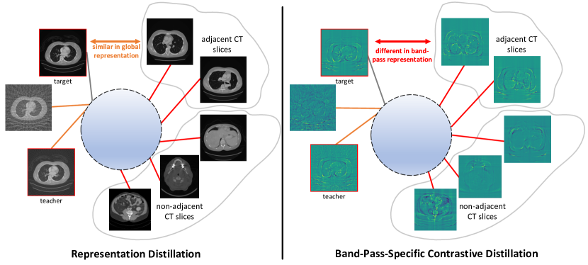
Figure 3: The difference between representation distillation (left) and band-pass-specific contrastive distillation (right). Global representation distillation fails to distinguish clinical details due to high similarity among similar body parts, e.g., adjacent lung slices. Band-pass-specific contrastive distillation further projects the representation to the DCT domain, enabling distillation of specific clinical details on corresponding DCT components.

Contrastive representation learning, as a self-supervised approach, encourages the model to maximize the difference among representations of different samples so that model can emphasize those category-specific representations. However, directly implementing these losses would lead to imprecise reconstruction results because most CT images are inherently similar in intensity distribution, especially for images of the same body parts, as shown in Fig. 3. Recent methods have achieved great success learning on specific DCT spectrum [18, 55, 51], due to its strong energy compaction property, making it simple to select specific frequency components [41]. Therefore, we distilled the image-specific details by applying contrastive distillation on specific discrete cosine transform (DCT) spectrums. On the one hand, detailed knowledge can be better distilled from specific frequency components of teacher GloRe. On the other hand, contrastive against different CT slices can further enhance image-specific details on corresponding DCT components.

Discrete cosine transform.

Discrete cosine transform (DCT) is widely used for data compression in low-frequency components. The basis function of 2D DCT is defined as follows:

$$B_{w,h}^{i,j}=\cos\left(\tfrac{\pi w}{N_{\mathrm{w}}}\left(i+\tfrac{1}{2}\right)\right)\cos\left(\tfrac{\pi h}{N_{\mathrm{h}}}\left(j+\tfrac{1}{2}\right)\right),$$ (4)

where $N_{\mathrm{w}}$ and $N_{\mathrm{h}}$ represent the width and height of the input, respectively. Then, 2D DCT of the latent feature $\bm{Z}$ can be written as:

$$f_{w,h}(\bm{Z})=\sum\nolimits_{i=0}^{N_{\mathrm{w}}-1}\sum\nolimits_{j=0}^{N_{\mathrm{h}}-1}[\bm{Z}]_{i,j}B_{w,h}^{i,j},$$ (5)

where $w\in\{0,1,\ldots,N_{\mathrm{w}}-1\},h\in\{0,1,\ldots,N_{\mathrm{h}}-1\}$. The $f(\bm{Z})\in\mathbb{R}^{N_{\mathrm{w}}\times N_{\mathrm{h}}}$ represents the 2D DCT frequency spectrum of $\bm{Z}$. Thus, frequency components can be easily selected by a mask $\bm{M}\in\{0,1\}^{N_{\mathrm{w}}\times N_{\mathrm{h}}}$.

Band-pass-specific contrastive distillation.

Crucially, the low-frequency components of GloRe contribute most to the reconstruction accuracy, while high-frequency may contain inherent noise and artifacts of CT images. We therefore use a band-pass supervised contrastive loss for the distillation, where a band-pass mask $\bm{M}$ is incorporated to filter out the mid-frequency part in the frequency domain, containing main structure as well as the necessary detail information. The proposed band-pass supervised contrastive loss can be written as:

$$\bm{z}=\texttt{flatten}\left(\texttt{crop}\left(f_{w,h}(\bm{Z}),\bm{M}\right)\right),$$ (6)

where crop operator will keep the value at locations where $\bm{M}=1$ while the flatten operator flattens the 2D spectrum map into 1D representation.

It is to be observed that the clinical details in the CT images vary from case by case and are each very critical for diagnosis, requiring more sophisticated instance-level distinction. To this end, we consider all representations from different CT slices as negative samples to maximize image-specific features while updating the memory bank $\mathcal{M}$ with the widely applied First-In-First-Out mechanism per iteration from the previous mini-batches. The proposed band-pass-specific contrastive distillation loss for sample $\bm{z}_{\mathrm{S}}$ can be written as follows:

$$\mathcal{L}_{\mathrm{bcd}}=-\log{\frac{\text{exp}\left(\bm{z}_{\mathrm{S}}^{\textrm{T}}\bm{z}_{\mathrm{T}}/\tau\right)}{\sum\nolimits_{\bm{z}\in\mathcal{M}}\text{exp}\left(\bm{z}_{\mathrm{S}}^{\textrm{T}}\bm{z}/\tau\right)}},$$ (7)

where $\bm{z}_{\mathrm{S}}$, $\bm{z}_{\mathrm{T}}$, and $\bm{z}$ are frequency representations of $\bm{Z}_{\mathrm{S}}$, $\bm{Z}_{\mathrm{T}}$, and negative samples from memory bank $\mathcal{M}$ of size $N_{\mathrm{mem}}$, respectively. $\tau$ is the temperature term used to adjust the sensitivity of negative samples.

3.5 Loss Function and Training Procedure

Teacher reconstruction.

To constrain the GloRe extracted from $\bm{I}_{\mathrm{S}}$ and $\bm{I}_{\mathrm{T}}$ in the same latent space, a naive solution is to share the same decoder in the training phase, which, however, brings instability. Therefore, we adopt the widely used Exponential Moving Average (EMA) with momentum $m$ to update the parameters $\theta$ of the teacher decoder by the student decoder [13]:

$$\theta_{\texttt{decoderT}}=m\theta_{\texttt{decoderT}}+(1-m)\theta_{\texttt{decoderS}}.$$ (8)

Then, the global representation $\bm{Z}_{\mathrm{T}}$ learned by the teacher is fed into to the decoder to obtain the teacher reconstruction result $\widehat{\bm{I}}_{\mathrm{T}}$, and we use $\ell_{1}$ loss to measure the pixel-wise difference between $\widehat{\bm{I}}_{\mathrm{T}}$ and the full-view ground-truth $\bm{I}_{\mathrm{F}}$ and train the teacher:

$$\mathcal{L}_{\mathrm{pixelT}}=\|\texttt{decoderT}({\bm{Z}}_{\mathrm{T}})-{\bm{I}}_{\mathrm{F}}\|_{1}.$$ (9)

Student reconstruction.

The pixel-wise error measurement for the student is defined in a similar way:

$$\mathcal{L}_{\mathrm{pixelS}}=\|\texttt{decoderS}(\bm{Z}_{\mathrm{S}})-\bm{I}_{\mathrm{F}}\|_{1}.$$ (10)

Finally, a compound loss function combining pixel-wise error and two distillation losses respectively defined in Eq. (3) and Eq. (7) is introduced for student network training to achieve high-quality sparse-view CT reconstruction:

$$\mathcal{L}_{\mathrm{Stu}}=\mathcal{L_{\mathrm{pixelS}}}+\alpha\mathcal{L}_{\mathrm{rdd}}+\beta\mathcal{L}_{\mathrm{bcd}},$$ (11)

GloReDi is trained following the process summarized in Algorithm 1, where the student and teacher encoder are trained iteratively.

Algorithm 1 The training process of GloReDi.

0:  encoderS, encoderT, decoderS, decoderT; Input images: $\bm{I}_{\mathrm{S}}$, $\bm{I}_{\mathrm{T}}$, $\bm{I}_{\mathrm{F}}$; momentum $m$ and Memory bank

1:  for $iter=0$ to $Max\_Iter$ do

2:     Update decoderT using Eq. (8)

3:     $\widehat{\bm{I}}_{\mathrm{T}},\bm{Z}_{\mathrm{T}}=\texttt{decoderT}(\texttt{encoderT}(\bm{I}_{\mathrm{T}}))$

4:     Optimize encoderT using Eq. (9)

5:     $\widehat{\bm{I}}_{\mathrm{S}},\bm{Z}_{\mathrm{S}}=\texttt{decoderS}(\texttt{encoderS}(\bm{I}_{\mathrm{S}}))$

6:     Optimize encoderS+decoderS using Eq. (11)

7:     Update memory bank

8:  end for

8:  encoderS+ decoderS

4 Experimental Results

	$N_{\mathrm{v}}$ = 18			$N_{\mathrm{v}}$ = 36			$N_{\mathrm{v}}$ = 72			$N_{\mathrm{v}}$ = 144
Methods	PSNR	SSIM	RMSE	PSNR	SSIM	RMSE	PSNR	SSIM	RMSE	PSNR	SSIM	RMSE
FBP	22.22	35.36	0.0795	25.49	47.49	0.0543	30.88	63.81	0.0293	37.12	82.94	0.0144
DDNet [59]	34.57	91.94	0.0187	38.24	94.91	0.0126	41.66	97.27	0.0083	46.75	98.79	0.0048
FBPConvNet [22]	35.95	93.62	0.0164	39.79	96.13	0.0106	43.76	97.47	0.0066	48.46	98.60	0.0039
DuDoNet [31]	35.69	93.96	0.0169	40.36	96.94	0.0103	44.86	98.39	0.0059	49.33	99.23	0.0036
DDPTrans [29]	35.11	93.48	0.0181	38.68	95.99	0.0121	43.56	98.16	0.0069	48.72	99.22	0.0038
DuDoTrans [47]	36.08	93.28	0.0161	40.75	96.67	0.0095	45.16	98.44	0.0057	49.96	99.28	0.0034
Fred-Net (ours)	38.08	95.20	0.0129	40.86	96.81	0.0093	44.43	98.18	0.0063	48.45	99.08	0.0039
GloReDi (ours)	38.65	95.87	0.0120	41.25	97.05	0.0090	45.18	98.43	0.0057	48.96	99.21	0.0037

Table 1: Quantitative evaluation [PSNR (db), SSIM (%) and RMSE] for state-of-the-art methods on DeepLesion dataset.

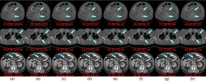
Figure 4: Visual comparison of state-of-the-art methods on DeepLesion dataset: (a) Ground Truth, (b) FBP, (c) DDNet, (d) FBPConvNet, (e) DuDoNet, (f) DDPTrans, (g) DuDoTrans, and (h) GloReDi. From top to bottom: the results under $N_{\mathrm{v}}=18,36,72$; display window is set to [-1000, 2000] HU for the first two rows and [-200, 300] HU for the third row.

4.1 Experimental Setup

Dataset.

We use DeepLesion dataset [54] and “2016 NIH-AAPM-Mayo Clinic Low-Dose CT Grand Challenge” AAPM dataset [35] to demonstrate the effectiveness of the proposed GloReDi. The DeepLesion dataset is the largest multi-lesion real-world CT dataset made available to the public, from which 40,000 images of 303 patients are selected as the training set while 1000 images of another 18 patients are selected as the test set. AAPM dataset contains routine dose CT data from 10 patients, where a total of 5,410 slices from 9 patients are chosen for training and 526 slices from the remaining 1 patient for testing. All images are resized to $256\times 256$. We simulate the forward and back projection using fan-beam geometry under 120 kVp and 500 mA with TorchRadon toolbox [43]. The distance from X-ray source to the rotation center is 59.5cm, and the number of detectors is set to 672. Sparse-view CT images are generated from $N_{\mathrm{v}}=18,36,72,144$ projection views uniformly sampled from full 720 views covering $[0,2\pi]$. To simulate the photon noise presented in real-world CT, an intensity of $1\times 10^{6}$ Poisson noise is added to the sinograms.

Implementation details.

Our model is implemented in PyTorch. We use Adam optimizer [24] with $(\beta_{1},\beta_{2})=(0.5,0.999)$ to train the model. The learning rate starts from $1\times 10^{-3}$ and is halved for every 40 epochs. For each method, four models of different $N_{\mathrm{v}}$ are trained separately on 4 NVIDIA RTX 3090 GPUs for 120 epochs with a batch size of 8. For hyperparameters in GloReDi, we set $\alpha$ and $\beta$ in Eq. (11) empirically to 0.1 and 0.0002 to fit the scale between losses. The momentum $m$ and temperature $\tau$ are set to 0.9 and 1.0, respectively, while the size $L$ of the memory bank is set to 300 to balance the performance and computational cost. We set intermediate-view as $N_{\mathrm{v}}\times 2$ by default. More details, including the network architecture, can be found in the Appendix.

Evaluation metrics.

For quantitative evaluation, we use peak signal-to-noise ratio (PSNR), structural similarity (SSIM) [61] and root mean square error (RMSE); all of them are widely adopted for image quality assessment.

	$N_{\mathrm{v}}$ = 18			$N_{\mathrm{v}}$ = 36			$N_{\mathrm{v}}$ = 72			$N_{\mathrm{v}}$ = 144
Methods	PSNR	SSIM	RMSE	PSNR	SSIM	RMSE	PSNR	SSIM	RMSE	PSNR	SSIM	RMSE
FBP	22.73	35.06	0.0732	26.27	47.52	0.0486	31.36	64.56	0.0270	37.85	84.57	0.0128
DDNet [59]	34.29	89.68	0.0194	36.95	93.03	0.0142	40.41	96.04	0.0096	44.35	98.05	0.0061
FBPConvNet [22]	35.73	92.84	0.0165	37.95	93.73	0.0127	42.92	97.19	0.0072	47.35	98.76	0.0043
DuDoNet [31]	34.82	93.00	0.0196	39.89	95.99	0.0102	44.06	98.02	0.0062	48.39	99.11	0.0038
DDPTrans [29]	34.47	91.95	0.0191	38.13	94.83	0.0125	42.77	97.65	0.0073	47.84	99.06	0.0041
DuDoTrans [47]	35.85	93.07	0.0162	40.04	96.02	0.0100	44.20	98.07	0.0062	49.02	99.21	0.0036
Fred-Net (ours)	37.20	93.90	0.0140	41.46	96.84	0.0085	43.64	97.84	0.0066	47.50	99.03	0.0042
GloReDi (ours)	37.91	94.58	0.0128	41.57	96.70	0.0084	44.24	98.03	0.0062	48.10	99.08	0.0040

Table 2: Quantitative evaluation [PSNR (db), SSIM (%) and RMSE] for state-of-the-art methods transferred to AAPM dataset.

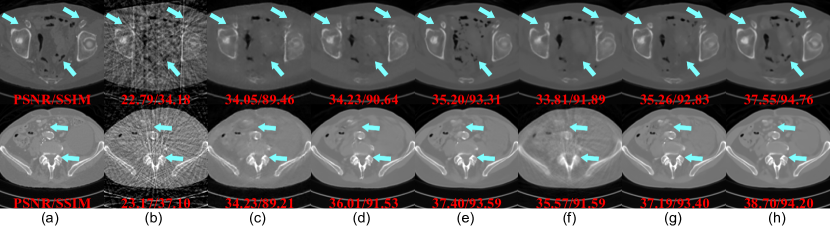
Figure 5: Visual comparison of state-of-the-art methods on AAPM dataset: (a) Ground Truth, (b) FBP, (c) DDNet, (d) FBPConvNet, (e) DuDoNet, (f) DDPTrans, (g) DuDoTrans, and (h) GloReDi. From top to bottom: $N_{\mathrm{v}}=18$, $36$; the display window is [-1000, 2000] HU.

4.2 Comparison with State-of-the-Art Methods

We compare GloReDi with the following state-of-the-art methods: DDNet [59], FBPConvNet [22], DuDoNet [31], DDPTrans [29], and DuDoTrans [47]. In addition, we name the network without the distillation from $\bm{I}_{\mathrm{T}}$ as the frequency encoder and decoder network (Fred-Net), optimized with only the pixel-wise loss in Eq. (10). FBP directly applies Radon transform to reconstruct the image from the sparse-view sinogram. DDNet and FBPConvNet are image-domain deep-learning methods taking FBP results as input. DuDoNet is a state-of-the-art dual-domain method that restores the CT image using two U-Nets in sinogram and image domains. Furthermore, DDPTrans and DuDoTrans adopt Transformer on both domains to restore the image by utilizing the long-range dependency. We try our best to reproduce these methods and then train and test them on the same dataset for a fair comparison.

Quantitative comparison.

Table 1 presents the quantitative comparison. Generally, dual-domain methods perform better than single domain methods, especially in the case of $N_{\mathrm{v}}=72,144$ thanks to the sinogram inpainting network. However, we highlight in ultra sparse-view scenarios where $N_{\mathrm{v}}=18$, that dual-domain methods like DuDoNet perform worse than classical image-domain-only methods such as FBPConvNet. This is mainly due to the secondary artifact introduced by the unsuccessful sinogram inpainting; e.g., when $N_{\mathrm{v}}=18$ in our setting, directly restoring the sinogram can be recognized as a 40$\times$ super-resolution task, which is rather challenging. Interestingly, DuDoTrans is superior to DuDoNet to some extent, indicating the importance of long-range dependency in sparse-view CT reconstruction. DDPTrans fails to surpass DuDoNet mainly because of the limited parameter number though most transformers are memory-consuming.

Compared with the previous works, the proposed GloReDi achieves competitive results by learning to distill GloRe for high-quality reconstruction. Particularly in ultra-sparse scenarios, e.g., when $N_{\mathrm{v}}=18$, GloReDi has 2.57db and 2.70db improvement on PSNR over DuDoTrans and FBPConvNet, respectively. As $N_{\mathrm{v}}$ increases, the advantage of GloReDi decreases, mainly due to a shift towards artifacts removal tasks rather than reconstruction. We highlight that the fewer projection views indicate less radiation dose and more speedup. We notice that global representation distillation further improves the performance of GloReDi from 0.51db to 0.89db compared to Fred-Net. The results show that the proposed GloReDi successfully inspire the potential of image post-processing methods and is significantly superior to the state-of-the-art methods under various settings.

Visual comparison.

Fig. A3 presents the visualization results of three sparse-view images. DDNet and FBPConvNet cannot remove the artifact thoroughly, while the reconstruction results are over-smooth in the boundary of organs and bones. Such effects can be easily observed in the second row of Figs. A3(c) and A3(d) on the spine where the anatomical structure is complicated. Although dual-domain methods perform better in general, we find that the accuracy in details is even worse than FBPConvNet in comparison with Figs. A3(d) and A3(e)-(g).

Among all these methods, GloReDi best recovers the structures and details, especially in ultra-sparse scenarios. As shown in the first two rows of Fig. A3(h), only GloReDi precisely reconstructs those clinically important details such as soft tissue and the corrupted pulmonary alveoli.

4.3 Ablation Study

We first evaluate the effectiveness of each component in GloReDi. We use Fred-Net as the baseline to add or remove components. The configurations involved in Table 3 are mainly four groups: (1) the baseline Fred-Net using pixel-wise loss to train student model without distillation components (a); (2) the baseline without Fourier convolutions (b–c); (3) the baseline with distillation from intermediate-view reconstructed images (d–g); and (4) the dual-domain version with raw data processed by sinogram-domain sub-network of DuDoNet [31] (h). Unless noted otherwise, pixel-wise loss is involved in training.

	config.	PSNR
a)	Fred-Net	38.09
b)	Fred-Net w/o Fourier	36.52
c)	Fred-Net w/o Fourier + $\mathcal{L}_{\mathrm{rdd}}$ + $\mathcal{L}_{\mathrm{bcd}}$	36.30
d)	Fred-Net + data augmentation	34.41
e)	Fred-Net + $\mathcal{L}_{\mathrm{rdd}}$	38.39
f)	Fred-Net + $\mathcal{L}_{\mathrm{bcd}}$	38.42
g)	Fred-Net + $\mathcal{L}_{\mathrm{rdd}}$ + $\mathcal{L}_{\mathrm{bcd}}$ = GloReDi	38.65
h)	Fred-Net + raw data	38.44

Table 3: Quantitative evaluation of different configurations.

Ablations on global representations.

The results between a) and b) in Table 3 confirm that learning global representations with the image-wide receptive field by Fourier convolution is beneficial for sparse CT reconstruction. Also, we notice that in Tables 1 and 2, our baseline Fred-Net still outperforms state-of-the-art methods when $N_{\mathrm{v}}=18$ and $36$. Interestingly, we found that c) performs even worse than b) in Table 3. This suggests that the global representation is essential for bridging the gap between images of different views. Generally, learning global representations is powerful and provides a new perspective for sparse-view CT reconstruction, which also answers that the limit of image post-processing methods is still far beyond reach.

Ablations on global representation distillation.

Through a comparison between Fred-Net and the one trained with intermediate-view images as data augmentation (a vs. d) in Table 3, we found that directly applying data augmentation had a negative impact, resulting in a 3.67db PSNR drop. This indicates that the network failed to benefit from denser-view images directly because of the significant domain gap among images of different view. By comparing a), e) and f) in Table 3, we can see that both e) representation directional distillation and f) band-pass-specific contrastive distillation can improve the performance of a), showing that end-to-end supervision cannot thoroughly unlock the potential of the GloRe. By training with both distillation loss, g) further boosts the performance and outperforms all other configurations. By comparing a), g) and h), we found unsurprisingly that using raw data does improve the performance of the image-domain network. However, our method GloReDi yields even better performance by effectively distilling GloRe from intermediate-view image data.

Ablations on intermediate views for distillation.

Selecting a suitable intermediate view for distillation is crucial in realizing the full potential of GloReDi. Images reconstructed from a denser view can provide richer information to the teacher GloRe while introducing a more significant domain gap. As presented in Table 4, we found that models distilled from $N_{\mathrm{v}}\times 2$ views exhibit the best performance. Interestingly, models distilled from the full-view image yield the worst performance, primarily because of the considerable domain gap between the input data.

Further ablation studies for framework designs, configurations of residual blocks, and ablation study for distillation loss can be found in the Appendix.

config.	$N_{\mathrm{v}}\times 2$	$N_{\mathrm{v}}\times 3$	$N_{\mathrm{v}}\times 4$	720
$N_{\mathrm{v}}=18$	38.38	38.29	38.28	38.02
$N_{\mathrm{v}}=72$	44.84	44.46	44.72	44.38

Table 4: PSNR evaluation of GloReDi trained with different intermediate-view images for 60 epochs. The first and second rows show the results of sparse-view images with $N_{\mathrm{v}}=18,72$ distilled from images of $N_{\mathrm{v}}\times 2,3,4$ and $720$ (full view), respectively.

4.4 Transfer to Other Dataset

To test the generalizability and robustness of GloReDi along with other state-of-the-art methods, we finetune each model for another ten epochs on AAPM dataset to bridge the domain gap following the same setting. In Table 2, the proposed GloReDi shows excellent transferability over all other state-of-the-art methods in (ultra) sparse-view scenarios ($N_{\mathrm{v}}=18,36,72$) and still achieves performance comparable with the dual-domain methods when $N_{\mathrm{v}}=72$. Specifically, when $N_{\mathrm{v}}=18$, we notice GloReDi has 2.06db and 2.18db improvements on PSNR compared to DuDotrans and FBPConvNet, respectively, indicating that our method is significantly superior in ultra sparse-view scenarios. Fig. A4 shows images with $N_{\mathrm{v}}=18$ and $36$, which are corrupted severely by FBP as shown in Fig. A4(b), thus losing its clinical value. Previous image-domain methods remove the artifact to some extent but lose most of the details, as shown in Figs. A4(c) and (d). Although the state-of-the-art dual-domain methods gain better results in general, we notice that clinical details such as lesion and bone, as pointed out by the blue arrows, are not accurately reconstructed in Figs. A4(e)-(g) while severe secondary artifacts are introduced, especially when $N_{\mathrm{v}}=18$. In contrast, the proposed GloReDi excels at reconstructing the details and greatly improves the clinical value of sparse-view CT.

5 Discussion and Conclusion

First, we emphasize that our contributions can be easily extended to dual-domain methods when sinogram data are available. On the one hand, learning to distill GloRe can also benefit the image-domain network in a dual-domain framework. On the other hand, the proposed method can also be used to enhance the sinogram recovery by distilling the sinogram with intermediate views. Future work can concentrate on extending GloReDi to dual domain methods and other CT reconstruction tasks, such as limited-views CT reconstruction and metal artifact reduction. Second, although the teacher network is trained alongside the student network in the current version, it is valuable to explore the utilization of pre-trained teacher models, enabling GloReDi to progressively distill the GloRe from a series of teacher models.

We also acknowledge some limitations. First, the teacher network will introduce additional computational costs during the training phase. It is possible to study how to distill knowledge from a pretrained teacher network. Second, although there are clear improvements in quantitative and visual results, it is desirable to have feedback from radiologists for clinical practice. The generalizability and robustness of the trained networks in clinical applications require further investigation. Third, we only considered 2D cases in the paper due to memory respect. If GPU memory permits, one can extend GloReDi to 3D by replacing 2D convolutions with 3D ones by applying high-dimension kernels for FFCs [7]. Lastly, GloReDi failed to surpass the dual-domain methods in denser view scenarios when sinogram can provide effective information for performance improvement. Studying how to improve the performance given an arbitrary $N_{\mathrm{v}}$ would be of great value for future research.

This paper sticks to reconstructing the sparse-view CT directly in the image domain by learning to distill global representation from intermediate-view reconstructed images innovatively. We propose to learn GloRe with Fourier convolution for image-wide receptive field and present directional and band-pass-specific contrastive distillation for high-quality reconstruction. The proposed framework GloReDi achieves state-of-the-art performance without access to sinogram data, demonstrating that the limit of the image post-processing methods is still far beyond reach.

Appendix

This Appendix includes five parts: (A) more ablation study and analysis, (B) efficiency, (C) more visualization results, and (D) detailed network architectures.

Appendix A More Ablation Study and Analysis

A.1 Ablation on Framework Design

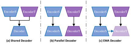
Figure A1: Framework designs of GloReDi: (a) GloReDi-S: shared decoder for student and teacher networks, which is optimized twice per iteration; (b) GloReDi-P: separate parallel decoders for student and teacher; and (c) GloReDi-E: teacher decoder is updated via EMA according to student decoder. For simplicity, we name GloReDi-E trained without distillation loss as GloReDi-N for comparison.

Table A1 presents the experimental results of different framework designs employed in GloReDi, as illustrated in Fig. A1. We found that the parallel decoder design failed to align the representations of different views into a shared latent space, thus, leading to suboptimal results. The result of GloReDi-P is even worse than GloReDi-N, revealing that the domain gap between various views can harm the training. Although the utilization of a shared decoder can enforce the representation to be in the same latent space and outperform GloReDi-P, it could also introduce unstable problems during training, for the parameters of the shared decoder are updated twice in an iteration. By contrast, GloReDi-E achieves the alignment of representations in a shared latent space through an exponential moving average (EMA) update procedure, thereby circumventing interference with student training. The resultant teacher encoder can be considered a stable version of the student encoder, making the teacher GloRe a dependable distillation target. Therefore, we choose GloReDi-E as our final framework design.

GloReDi	-N	-P	-S	-E
PSNR	37.91	37.85	38.04	38.38

Table A1: PSNR evaluation of GloReDi with different framework designs. All networks are trained under $N_{\mathrm{v}}=18$ for 60 epochs.

A.2 Ablation on Configurations of Residual Blocks

config.	e5d4	e6d3	e7d2	e8d1
$N_{\mathrm{v}}=18$	37.49	37.62	38.06	38.02
$N_{\mathrm{v}}=72$	43.75	43.90	44.39	44.08

Table A2: PSNR evaluation of GloReDi with varied numbers of FFC residual blocks in the encoder and decoder. (e.g., e5d4 represents 5 and 4 FFC residual blocks in the encoder and decoder, respectively). All models are trained for 40 epochs considering the computational cost.

Given the fixed parameters, a larger encoder can improve the information extraction and recovery process, as well as better bridge the domain gap between the sparse- and denser-view images. In the meantime, a larger decoder can better decode the global representation and improve the reconstruction quality. Table A2 presents the quantitative results of varying numbers of FFC residual blocks in the encoder and decoder. The results suggest that a ratio of $7:2$ for 9 residual blocks in the encoder and decoder is the most favorable for distillation.

A.3 Ablation on Distillation Loss

config.	$\ell_{1}$ loss	$\ell_{2}$ loss	(ours)
$N_{\mathrm{v}}=18$	37.44	37.29	38.06
$N_{\mathrm{v}}=72$	42.88	42.56	44.39

Table A3: PSNR evaluation of GloReDi trained with different distillation loss, including $\ell_{1}$ loss and $\ell_{2}$ loss commonly used in knowledge distillation, as well as the proposed one with $\mathcal{L}_{\mathrm{rdd}}$ and $\mathcal{L}_{\mathrm{bcd}}$. All models are trained for 40 epochs considering the computational cost.

Table A3 exhibits the results of GloReDi trained with different distillation loss. Our findings suggest that pixel-wise distillation losses, such as $\ell_{1}$ and $\ell_{2}$ loss, are not as effective as the proposed one. This is attributed to the fact that conventional distillation tasks involve both the student and teacher networks sharing the same input and ground truth. Consequently, the domain gap does not affect them. However, for sparse-view CT reconstruction, it is arduous for the student to recover the missing information entirely. This renders pixel-wise losses too abrupt for distillation purposes.

A.4 Ablation on Band-pass-specific Contrastive Distillation

We have demonstrated the effective components by training GloReDi with $\mathcal{L}_{\mathrm{bcd}}$ on specific frequency components. However, there are various methods to split the frequency components [18, 39, 55, 51]. Note that in 2D discrete cosine transform, low-frequency components are placed on the upper left. We define the mask $\bm{M}\in\{0,1\}^{N_{\mathrm{w}}\times N_{\mathrm{h}}}$ as follows to select the target components:

$$\bm{M}_{i,j}=\begin{cases}1,\text{if}\ i\!\in\![b_{\mathrm{low}}N_{\mathrm{w}},b_{\mathrm{up}}N_{\mathrm{w}}]\ \text{and}\ j\!\in\![b_{\mathrm{low}}N_{\mathrm{h}},b_{\mathrm{up}}N_{\mathrm{h}}]\\ 0,\text{otherwise,}\end{cases}$$ (A.1)

where $\bm{M}_{i,j}$ is the element in $\bm{M}$ at position $(i,j)$; $b_{\mathrm{low}}$ and $b_{\mathrm{up}}$ denote the hand-craft ratios defining the lower and upper bounds, respectively, which range from $[0,1]$. We then split the DCT spectrum into five groups, demarcated by the intervals $[b_{\mathrm{low}},b_{\mathrm{up}}]$, as illustrated in Fig. A2. Notably, the model distilled via the vanilla supervised contrastive loss served as the baseline for our comparative analysis and was denoted by the black horizontal line in Fig. A2.

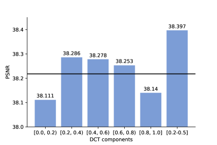
Figure A2: The effect of different frequency components. Note that the black horizontal line represents the contrastive distillation without projecting the representation to the DCT domain. The models are trained with $\mathcal{L}_{\mathrm{bcd}}$ only for 60 epochs.

Obviously, models trained with frequency components, except for the lowest and highest, perform better than vanilla ones, demonstrating that selecting band-pass components is effective. In addition, middle groups perform relatively better among different groups, demonstrating the effectiveness of the selected band-pass-specific components. Therefore, we select $[b_{\mathrm{low}},b_{\mathrm{up}}]=[0.2,0.5]$ to train our final models to balance the performance and memory usage.

Appendix B Efficiency

Methods	DDNet	FBPConvNet	DuDoNet	DDPTrans	DuDoTrans	GloReDi
mem. (MB)	86.4	274.9	2150.1	7220.3	3108.5	798.8
infer. (ms)	14.7	11.7	49.6	71.3	78.4	33.1

Table A4: Peak memory usage and mean inference time on a single RTX 3090 GPU using 1000 images, with a batch size of 1, at a resolution of $256\times 256$.

Table A4 presents the peak memory usage (mem.) and mean inference time (infer.) assessed on a single RTX 3090 GPU with a batch size of 1, averaging over 1000 images at a resolution of $256\times 256$. Overall, dual-domain methods exhibit lower efficiency compared to image post-processing techniques. Transformer-based methods are suboptimal in both memory usage and inference time to those built with CNN. In contrast, GloReDi demonstrates comparable performance to other post-processing methods while achieving higher efficiency than dual-domain approaches by eliminating the need for the teacher network during inference.

Appendix C More Visualization Results

Fig. A3 presents the visualization results of six groups of sparse-view images. Among all the methods, GloReDi better recovers the clinical details such as the lung trachea in the first row, the round soft tissue in the second row, and the clear boundary highlighted in the fifth row.

Fig. A4 shows another four images in the AAPM dataset. We note that in ultra-sparse scenarios when $N_{\mathrm{V}}=18,36$ as shown in the first and the second rows, only GloReDi precisely reconstructs the structure highlighted by the blue box. When $N_{\mathrm{V}}=72$, GloReDi achieves competitive performance compared with DuDoTrans but without using the sinogram data.

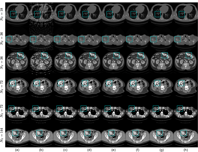
Figure A3: Visual comparison of state-of-the-art methods on DeepLesion dataset: (a) Ground Truth, (b) FBP, (c) DDNet, (d) FBPConvNet, (e) DuDoNet, (f) DDPTrans, (g) DuDoTrans, and (h) GloReDi. From top to bottom: the results under $N_{\mathrm{v}}=18,36,36,72,72,144$; display window is set to [-1000, 2000] HU for the first and the second rows, and [-200, 300] HU for the rests.

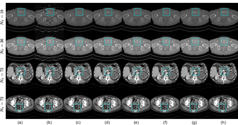
Figure A4: Visual comparison of state-of-the-art methods on AAPM dataset: (a) Ground Truth, (b) FBP, (c) DDNet, (d) FBPConvNet, (e) DuDoNet, (f) DDPTrans, (g) DuDoTrans, and (h) GloReDi. From top to bottom: the results under $N_{\mathrm{v}}=18,36,72,72$; display window is set to [-1000, 2000] HU for the first row, [-1000, 1000]HU for the second row and [-200, 300] HU for the third and fourth row.

Appendix D Detailed Network Architectures

Tables A5 and A6 show the detailed network architecture of the encoder and decoder, respectively.

Name	Channels	Description
Input	2	sparse-view images $\bm{I}_{\mathrm{S}}$ or $\bm{I}_{\mathrm{T}}$
Rpad0	2	reflectionpad2d((3,3,3,3))
Down1	64	K7C64S1P1-BN-ReLU
Down2	128	K3C128S2P1-BN-ReLU
FFC-Split $\times m$	256	local branch: K3C64S2P1-BN-ReLU global branch: K3C192S2P1-BN-ReLU
FFC-1 $\times m$	256	convl2l: K3C64S1P1 convl2g: K3C192S1P1 convg2l: K3C64S1P1 convg2g: K1C96S1-bn-relu-FFT-K1C192S1-iFFT-K1C192S1 local branch: BN-ReLU global branch: BN-ReLU
FFC-2 $\times m$	256	convl2l: K3C64S1P1 convl2g: K3C192S1P1 convg2l: K3C64S1P1 convg2g: K1C96S1-bn-relu-FFT-K1C192S1-iFFT-K1C192S1 local branch: BN-ReLU global branch: BN-ReLU
FFC-Cat $\times m$	256	concat(local branch, global branch) w/ residual learning

Table A5: Network architecture of student and teacher encoder. We use ‘K-C-S-P’ to denote the kernel, channel, stride, and padding configuration of convolution layers.

Name	Channels	Description
FFC-Split $\times n$	256	local branch: K3C64S2P1-BN-ReLU global branch: K3C192S2P1-BN-ReLU
FFC-1 $\times n$	256	convl2l: K3C64S1P1 convl2g: K3C192S1P1 convg2l: K3C64S1P1 convg2g: K1C96S1-bn-relu-FFT-K1C192S1-iFFT-K1C192S1 local branch: BN-ReLU global branch: BN-ReLU
FFC-2 $\times n$	256	convl2l: K3C64S1P1 convl2g: K3C192S1P1 convg2l: K3C64S1P1 convg2g: K1C96S1-bn-relu-FFT-K1C192S1-iFFT-K1C192S1 local branch: BN-ReLU global branch: BN-ReLU
FFC-Cat $\times n$	256	concat(local branch, global branch) w/ residual learning
Up1	128	ConvTranspose2d: K3C128S2P1-BN-ReLU
Up2	64	ConvTranspose2d: K3C64S2P1-BN-ReLU
Rpad1	64	reflectionpad2d((3,3,3,3))
Out	1	K7C1S1

Table A6: Network architecture of the shared decoder. We use ‘K-C-S-P’ to denote the kernel, channel, stride, and padding configuration of convolution layers.

References

- [1] Jielin Bai, Yitong Liu, and Hongwen Yang. Sparse-view CT reconstruction based on a hybrid domain model with multi-level wavelet transform. Sensors, 22(9):3228, 2022.
- [2] Gregory A Baxes. Digital image processing: principles and applications. John Wiley & Sons, Inc., 1994.
- [3] Mu Cai, Hong Zhang, Huijuan Huang, Qichuan Geng, Yixuan Li, and Gao Huang. Frequency domain image translation: More photo-realistic, better identity-preserving. In Proceedings of the IEEE/CVF International Conference on Computer Vision, pages 13930–13940, 2021.
- [4] Guang-Hong Chen, Jie Tang, and Leng Shuai. Prior image constrained compressed sensing (PICCS): A method to accurately reconstruct dynamic CT images from highly undersampled projection data sets. Medical Physics, 35(2):660–663, 2008.
- [5] Hu Chen, Yi Zhang, Mannudeep K. Kalra, Feng Lin, Yang Chen, Peixi Liao, Jiliu Zhou, and Ge Wang. Low-dose CT with a residual encoder-decoder convolutional neural network. IEEE Transactions on Medical Imaging, 36(12):2524–2535, 2017.
- [6] Theodor Cheslerean-Boghiu, Felix C. Hofmann, Manuel Schultheiss, Franz Pfeiffer, Daniela Pfeiffer, and Tobias Lasser. WNet: A data-driven dual-domain denoising model for sparse-view computed tomography with a trainable reconstruction layer. IEEE Transactions on Computational Imaging, 9:120–132, 2022.
- [7] Lu Chi, Borui Jiang, and Yadong Mu. Fast Fourier convolution. In Advances in Neural Information Processing Systems, volume 33, pages 4479–4488, 2020.
- [8] Hao Fu, Shaojun Zhou, Qihong Yang, Junjie Tang, Guiquan Liu, Kaikui Liu, and Xiaolong Li. Lrc-bert: latent-representation contrastive knowledge distillation for natural language understanding. In Proceedings of the AAAI Conference on Artificial Intelligence, volume 35, pages 12830–12838, 2021.
- [9] Yue Gao, Fangyun Wei, Jianmin Bao, Shuyang Gu, Dong Chen, Fang Wen, and Zhouhui Lian. High-fidelity and arbitrary face editing. In Proceedings of the IEEE/CVF conference on computer vision and pattern recognition, pages 16115–16124, 2021.
- [10] Muhammad Usman Ghani and W. Clem Karl. Deep learning-based sinogram completion for low-dose CT. In 2018 IEEE 13th Image, Video, and Multidimensional Signal Processing Workshop, pages 1–5, 2018.
- [11] Fatemeh Haghighi, Mohammad Reza Hosseinzadeh Taher, Michael B. Gotway, and Jianming Liang. DiRA: Discriminative, restorative, and adversarial learning for self-supervised medical image analysis. In Proceedings of the IEEE/CVF Conference on Computer Vision and Pattern Recognition, pages 20824–20834, 2022.
- [12] Ji He, Yan Yang, Yongbo Wang, Dong Zeng, Zhaoying Bian, Hao Zhang, Jian Sun, Zongben Xu, and Jianhua Ma. Optimizing a parameterized plug-and-play ADMM for iterative low-dose CT reconstruction. IEEE Transactions on Medical Imaging, 38(2):371–382, 2019.
- [13] Kaiming He, Haoqi Fan, Yuxin Wu, Saining Xie, and Ross Girshick. Momentum contrast for unsupervised visual representation learning. In Proceedings of the IEEE/CVF conference on computer vision and pattern recognition, pages 9729–9738, 2020.
- [14] Zibin He, Tao Dai, Jian Lu, Yong Jiang, and Shu-Tao Xia. Fakd: Feature-affinity based knowledge distillation for efficient image super-resolution. In 2020 IEEE International Conference on Image Processing (ICIP), pages 518–522, 2020.
- [15] Geoffrey Hinton, Oriol Vinyals, and Jeff Dean. Distilling the knowledge in a neural network. arXiv preprint arXiv:1503.02531, 2015.
- [16] Ming Hong, Yuan Xie, Cuihua Li, and Yanyun Qu. Distilling image dehazing with heterogeneous task imitation. In Proceedings of the IEEE/CVF Conference on Computer Vision and Pattern Recognition, pages 3462–3471, 2020.
- [17] Dianlin Hu, Jin Liu, Tianling Lv, Qianlong Zhao, Yikun Zhang, Guotao Quan, Juan Feng, Yang Chen, and Limin Luo. Hybrid-domain neural network processing for sparse-view CT reconstruction. IEEE Transactions on Radiation and Plasma Medical Sciences, 5(1):88–98, 2020.
- [18] Jiaxing Huang, Dayan Guan, Aoran Xiao, and Shijian Lu. FSDR: Frequency space domain randomization for domain generalization. In Proceedings of the IEEE/CVF Conference on Computer Vision and Pattern Recognition, pages 6891–6902, 2021.
- [19] Zhizhong Huang, Jie Chen, Junping Zhang, and Hongming Shan. Learning representation for clustering via prototype scattering and positive sampling. IEEE Transactions on Pattern Analysis and Machine Intelligence, 2022.
- [20] Zhizhong Huang, Junping Zhang, Yi Zhang, and Hongming Shan. Du-gan: Generative adversarial networks with dual-domain u-net-based discriminators for low-dose CT denoising. IEEE Transactions on Instrumentation and Measurement, 71:1–12, 2021.
- [21] Shuai Jia, Chao Ma, Taiping Yao, Bangjie Yin, Shouhong Ding, and Xiaokang Yang. Exploring frequency adversarial attacks for face forgery detection. In Proceedings of the IEEE/CVF Conference on Computer Vision and Pattern Recognition, pages 4103–4112, 2022.
- [22] Kyong Hwan Jin, Michael T McCann, Emmanuel Froustey, and Michael Unser. Deep convolutional neural network for inverse problems in imaging. IEEE Transactions on Image Processing, 26(9):4509–4522, 2017.
- [23] Kyungsang Kim, Jong Chul Ye, William Worstell, Jinsong Ouyang, Yothin Rakvongthai, Georges El Fakhri, and Quanzheng Li. Sparse-view spectral CT reconstruction using spectral patch-based low-rank penalty. IEEE Transactions on Medical Imaging, 34(3):748–760, 2015.
- [24] Diederik P. Kingma and Jimmy Ba. Adam: A method for stochastic optimization. arXiv preprint arXiv:1412.6980, 2014.
- [25] Hoyeon Lee, Jongha Lee, Hyeongseok Kim, Byungchul Cho, and Seungryong Cho. Deep-neural-network-based sinogram synthesis for sparse-view CT image reconstruction. IEEE Transactions on Radiation and Plasma Medical Sciences, 3(2):109–119, 2018.
- [26] Minjae Lee, Hyemi Kim, and Hee-Joung Kim. Sparse-view CT reconstruction based on multi-level wavelet convolution neural network. Physica Medica, 80:352–362, 2020.
- [27] Wonkyung Lee, Junghyup Lee, Dohyung Kim, and Bumsub Ham. Learning with privileged information for efficient image super-resolution. In Computer Vision–ECCV 2020: 16th European Conference, Glasgow, UK, August 23–28, 2020, Proceedings, Part XXIV 16, pages 465–482, 2020.
- [28] Jiaming Li, Hongtao Xie, Jiahong Li, Zhongyuan Wang, and Yongdong Zhang. Frequency-aware discriminative feature learning supervised by single-center loss for face forgery detection. In Proceedings of the IEEE/CVF Conference on Computer Vision and Pattern Recognition, pages 6458–6467, 2021.
- [29] Runrui Li, Qing Li, Hexi Wang, Saize Li, Juanjuan Zhao, Yan Qiang, and Long Wang. DDPTransformer: Dual-domain with parallel transformer network for sparse view CT image reconstruction. IEEE Transactions on Computational Imaging, pages 1–15, 2022.
- [30] Zilong Li, Qi Gao, Yaping Wu, Chuang Niu, Junping Zhang, Meiyun Wang, Ge Wang, and Hongming Shan. Quad-Net: Quad-domain network for CT metal artifact reduction. arXiv preprint arXiv:2207.11678, 2023.
- [31] Wei-An Lin, Cheng Liao, Haofu abd Peng, Xiaohang Sun, Jingdan Zhang, Jiebo Luo, Rama Chellappa, and Zhou S. Kevin. DuDoNet: Dual domain network for CT metal artifact reduction. In Proceedings of the IEEE/CVF Conference on Computer Vision and Pattern Recognition, pages 10512–10521, 2019.
- [32] Pengju Liu, Hongzhi Zhang, K. Zhang, Liang Lin, and Wangmeng Zuo. Multi-level wavelet-cnn for image restoration. 2018 IEEE/CVF Conference on Computer Vision and Pattern Recognition Workshops (CVPRW), pages 886–88609, 2018.
- [33] Yi Liu, Shangguan Hong, Quan Zhang, Hongqing Zhu, Huazhong Shu, and Zhiguo Gui. Median prior constrained TV algorithm for sparse view low-dose CT reconstruction. Computers in Biology and Medicine, 60:117–131, 2015.
- [34] Chenglong Ma, Zilong Li, Junping Zhang, Yi Zhang, and Hongming Shan. FreeSeed: Frequency-band-aware and self-guided network for sparse-view CT reconstruction. arXiv preprint arXiv:2307.05890, 2023.
- [35] C. McCollough. TU-FG-207A-04: Overview of the low dose CT grand challenge. Medical Physics, 43(6):3759–3760, 2016.
- [36] Donald L Miller and David Schauer. The alara principle in medical imaging. Philosophy, 44:595–600, 1983.
- [37] Shanzhou Niu, Yang Gao, Zhaoying Bian, Jing Huang, Wufan Chen, Gaohang Yu, Zhengrong Liang, and Jianhua Ma. Sparse-view X-ray CT reconstruction via total generalized variation regularization. Physics in Medicine and Biology, 59(12):2997–3017, 2014.
- [38] SeongUk Park and Nojun Kwak. Local-selective feature distillation for single image super-resolution. arXiv preprint arXiv:2111.10988, 2021.
- [39] Zequn Qin, Pengyi Zhang, Fei Wu, and Xi Li. Fcanet: Frequency channel attention networks. In Proceedings of the IEEE/CVF international conference on computer vision, pages 783–792, 2021.
- [40] J. Radon. Über die Bestimmung von Funktionen durch ihre Integralwerte längs gewisser Mannigfaltigkeiten. Berichtë uber die Verhandlungen der Köberniglich-Säberchsischen Akademie der Wissenschaften zu Leipzig, 69:262–277, 1917.
- [41] K Ramamohan Rao and Ping Yip. Discrete cosine transform: algorithms, advantages, applications. Academic press, 2014.
- [42] Adriana Romero, Nicolas Ballas, Samira Ebrahimi Kahou, Antoine Chassang, Carlo Gatta, and Yoshua Bengio. Fitnets: Hints for thin deep nets. arXiv preprint arXiv:1412.6550, 2014.
- [43] Matteo Ronchetti. TorchRadon: Fast differentiable routines for computed tomography. arXiv preprint arXiv:2009.14788, 2020.
- [44] Roman Suvorov, Elizaveta Logacheva, Anton Mashikhin, Anastasia Remizova, Arsenii Ashukha, Aleksei Silvestrov, Naejin Kong, Harshith Goka, Kiwoong Park, and Victor Lempitsky. Resolution-robust large mask inpainting with Fourier convolutions. In 2022 IEEE/CVF Winter Conference on Applications of Computer Vision, pages 2149–2159, 2022.
- [45] Yonglong Tian, Dilip Krishnan, and Phillip Isola. Contrastive representation distillation. arXiv preprint arXiv:1910.10699, 2019.
- [46] Ashish Vaswani, Noam Shazeer, Niki Parmar, Jakob Uszkoreit, Llion Jones, Aidan N. Gomez, Łukasz Kaiser, and Illia Polosukhin. Attention is all you need. In Proceedings of the 31st International Conference on Neural Information Processing Systems, pages 6000–6010, 2017.
- [47] Ce Wang, Kun Shang, Haimiao Zhang, Qian Li, and S. Kevin Zhou. DuDoTrans: Dual-domain transformer for sparse-view CT reconstruction. In Machine Learning for Medical Image Reconstruction, pages 84–94. Springer International Publishing, 2022.
- [48] Ge Wang, Hengyong Yu, and Bruno De Man. An outlook on X-ray CT research and development. Medical Physics, 35(3):1051–1064, 2008.
- [49] Lin Wang and Kuk-Jin Yoon. Knowledge distillation and student-teacher learning for visual intelligence: A review and new outlooks. IEEE transactions on pattern analysis and machine intelligence, 44(6):3048–3068, 2021.
- [50] Wenjun Xia, Ziyuan Yang, Zexin Lu, Zhongxian Wang, and Yi Zhang. Regformer: A local-nonlocal regularization-based model for sparse-view CT reconstruction. IEEE Transactions on Radiation and Plasma Medical Sciences, pages 1–1, 2023.
- [51] Wenbin Xie, Dehua Song, Chang Xu, Chunjing Xu, Hui Zhang, and Yunhe Wang. Learning frequency-aware dynamic network for efficient super-resolution. In Proceedings of the IEEE/CVF International Conference on Computer Vision, pages 4308–4317, 2021.
- [52] Moran Xu, Dianlin Hu, Fulin Luo, Fenglin Liu, Shaoyu Wang, and Weiwen Wu. Limited-angle X-ray CT reconstruction using image gradient -norm with dictionary learning. IEEE Transactions on Radiation and Plasma Medical Sciences, 5:78–87, 2021.
- [53] Sidky Emil Y., Chien-Min Kao, and Xiaochuan Pan. Accurate image reconstruction from few-views and limited-angle data in divergent-beam ct. Journal of X-Ray Science and Technology, 14(2):119–139, 2006.
- [54] Ke Yan, Xiaosong Wang, Le Lu, and Ronald M. Summers. DeepLesion: Automated mining of large-scale lesion annotations and universal lesion detection with deep learning. Journal of Medical Imaging, 5(3):036501, 2018.
- [55] Yanchao Yang and Stefano Soatto. FDA: Fourier domain adaptation for semantic segmentation. In Proceedings of the IEEE/CVF Conference on Computer Vision and Pattern Recognition, pages 4085–4095, 2020.
- [56] Jaejun Yoo, Youngjung Uh, Sanghyuk Chun, Byeongkyu Kang, and Jung-Woo Ha. Photorealistic style transfer via wavelet transforms. In Proceedings of the IEEE/CVF International Conference on Computer Vision, pages 9036–9045, 2019.
- [57] Jingyi Zhang, Jiaxing Huang, Zichen Tian, and Shijian Lu. Spectral unsupervised domain adaptation for visual recognition. In Proceedings of the IEEE/CVF Conference on Computer Vision and Pattern Recognition, pages 9829–9840, 2022.
- [58] Yi Zhang, Hu Chen, Wenjun Xia, Yang Chen, Baodong Liu, Yan Liu, Huaiqiang Sun, and Jiliu Zhou. Learn++: recurrent dual-domain reconstruction network for compressed sensing CT. IEEE Transactions on Radiation and Plasma Medical Sciences, 7(2):132–142, 2022.
- [59] Zhicheng Zhang, Xiaokun Liang, Xu Dong, Yaoqin Xie, and Guohua Cao. A sparse-view CT reconstruction method based on combination of DenseNet and deconvolution. IEEE Transactions on Medical Imaging, 37(6):1407–1417, 2018.
- [60] Yijie Zhong, Bo Li, Lv Tang, Senyun Kuang, Shuang Wu, and Shouhong Ding. Detecting camouflaged object in frequency domain. In Proceedings of the IEEE/CVF Conference on Computer Vision and Pattern Recognition, pages 4504–4513, 2022.
- [61] Wang Zhou, Alan Conrad Bovik, Hamid Rahim Sheikh, and Eero P Simoncelli. Image quality assessment: from error visibility to structural similarity. IEEE Transactions on Image Processing, 13(4), 2004.